Newton’s Laws MONDAY, September 14, Re-introduction to Newton’s 3 Laws.
Laboratory Report Scoring and Cover Sheet
Title of Lab _Newton’s Laws______________________________________________________________
Course and Lab Section Number: PHY ___1103__- __100__ Date _23 Sept 2014________________
Principle Investigator _Thomas Edison______________________________________________________
Co-Investigator _Nikola Tesla_____________________________________________________________
5 3-4 0-2 Comments
Format N/A
Title Page N/A N/A
Abstract N/A
Introduction / Materials and Methods
PI Score _________ + 15 = _________ / 30
Results
Discussion: Data and Error Analysis
Discussion: Conclusion
Co-I Score _________ + 15 = _________ / 30
2
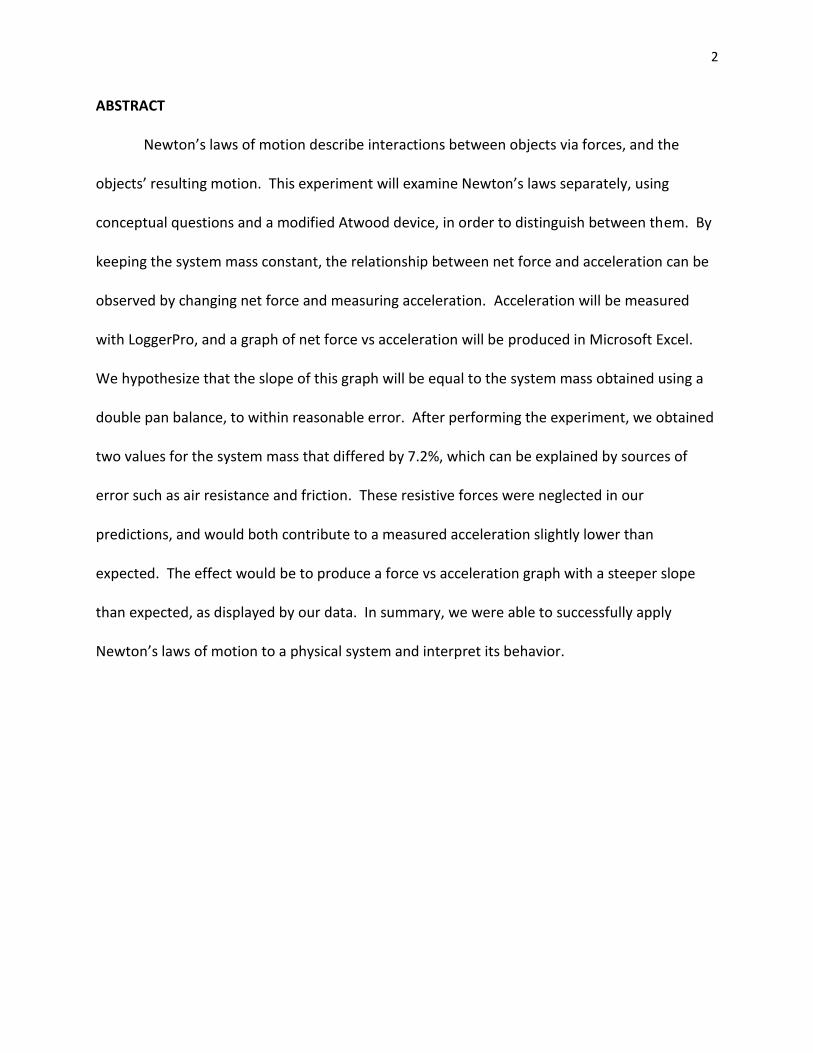
ABSTRACT
Newton’s laws of motion describe interactions between objects via forces, and the
objects’ resulting motion. This experiment will examine Newton’s laws separately, using
conceptual questions and a modified Atwood device, in order to distinguish between them. By
keeping the system mass constant, the relationship between net force and acceleration can be
observed by changing net force and measuring acceleration. Acceleration will be measured
with LoggerPro, and a graph of net force vs acceleration will be produced in Microsoft Excel.
We hypothesize that the slope of this graph will be equal to the system mass obtained using a
double pan balance, to within reasonable error. After performing the experiment, we obtained
two values for the system mass that differed by 7.2%, which can be explained by sources of
error such as air resistance and friction. These resistive forces were neglected in our
predictions, and would both contribute to a measured acceleration slightly lower than
expected. The effect would be to produce a force vs acceleration graph with a steeper slope
than expected, as displayed by our data. In summary, we were able to successfully apply
Newton’s laws of motion to a physical system and interpret its behavior.

3
INTRODUCTION
Newton’s laws of motion describe the effects of forces on an object’s or system’s
motion. In brief, if the vector sum of all forces acting on a system is unbalanced, then the
system will accelerate in a manner governed by the net force and the mass of the system.
First Law – Newton’s first law states that, in the absence of a net force, a system will
have no acceleration. For example, an object falling at terminal velocity is subject to two main
forces; gravity exerts a force toward the earth’s surface, and air resistance exerts a force in the
opposite direction. At terminal velocity, the force from air resistance is equal in magnitude to
the gravitational force and opposite in direction. Thus there is no net force on the falling
object, and its velocity is constant.
Second Law – When a system is subject to a nonzero net force, it accelerates. Newton’s
second law describes this acceleration in terms of the mass of the system and the net force:
Eq. 1
Thus, for a given mass, a larger force will produce a greater acceleration. Likewise, for a given
force, a larger mass will experience a smaller acceleration.
Third Law – Forces do not materialize out of thin air; Newton’s third law addresses this.
The weight of a chair is a force acting on the floor beneath it. If the floor did not exert a force
equal in magnitude and opposite in direction on the chair, the chair would accelerate in some
direction, according to Newton’s first law. Two objects that share a force in this manner may
be called an action-reaction force pair.
This experiment used a modified Atwood device to examine Newton’s laws of motion,
as described below.

4
Figure 1a: Modified Atwood device Figure 1b: Forces considered in this experiment
The modified Atwood device used consisted of a low-friction cart on a level track,
connected to a hanging mass by a string. The string had a paper clip on either end, and was fed
over a low-friction pulley, as shown in Figure 1a. The forces considered to be acting on the
system are shown in Figure 1b above. Air resistance and friction were neglected.
Several action-reaction force pairs are apparent from Figure 1b. First, the cart is pulled
toward the earth via gravitation. Likewise, the earth is pulled toward the cart, but with a much
smaller acceleration. Opposing the weight of the cart (although not its force pair) is the normal
force exerted on the cart by the track. It is paired with an equal and opposite contact force
exerted by the cart. The two tension forces are also a third law pair, although they constitute
an internal force, and are in effect equal and opposite.
Without the tension force acting horizontally on the cart, it remains stationary on the
track. Thus the normal force and the weight (m1g) of the cart must cancel. Both tension forces
are internal, and cancel as well. Therefore the net force on the system is produced exclusively
by the weight (m2g) of the hanging mass. Substituting into Eq. 1:
( ) Eq. 2

5
The purpose of this experiment is to examine and verify Newton’s laws of motion
empirically. Eq. 2 above is in linear form y = mx + b, where dependent variable (y) is the net
force (m2g), slope (m) is the system mass (m1 + m2), independent variable (x) is the acceleration
(a) of the system, and intercept (b) is zero. Force and acceleration are the independent and
dependent variables, respectively, and would normally be graphed a vs. F. However, for this
experiment they were graphed F vs. a, in order to have a slope equal to the system mass.
We hypothesize that we will be able to determine the system mass graphically in this
manner, to within reasonable error, having measured the hanging mass and the acceleration of
the system. We expect the vertical intercept to be zero; in the context of Newton’s first law,
zero net force will produce zero acceleration. We expect our calculated system mass to be
slightly larger than the value obtained using a double pan balance, due mainly to air resistance
and internal friction. These are neglected in Eq. 2 and will cause measured acceleration to be
slightly less than expected, making the slope of the graph steeper.

6
MATERIALS
computer with LoggerPro and Microsoft Excel
Go!Motion Vernier motion detector
low-friction cart with track
low-friction pulley
cotton string and two paper clips
two 0.020 kg masses
two 0.010 kg masses
two 0.200 kg masses
double pan balance
Figure 2: Experimental Setup for Modified Atwood Device
motion detector cart and masses
hanging mass
pulley
computer with LoggerPro
and Microsoft Excel
track
string

7
METHODS
Activity 1: Newton’s First and Third Laws
The cart was placed on the track, and the four small masses and paper clips and string
were placed atop it. The forces acting on the system were the gravitational force on the cart
and objects atop it, and the normal force from the track opposing the cart’s weight. The net
force on the system was zero. Thus there was no imbalance of forces, and no acceleration.
One end of the string was attached to the cart with a paper clip, while the other end of
the string was fed over the pulley. While keeping three masses atop the cart, one 0.020 kg
mass was hung from the vertical end of the string with the second paper clip. It was observed
that when released, the system accelerates (hanging mass toward the floor, cart toward the
pulley). The forces acting on the system are those shown in Figure 1b above. The net force
acting on the system is the weight of the hanging mass, given by m2g = (0.020 kg)(9.7953 m/s2)
= 0.195906 N = 0.20 N. The system is now accelerating because there is an imbalance of force,
as described by Newton’s first law.
The following questions, taken from the lab web page examine third law force pairs:
1. If not the normal force, what is the force that is equal and opposite to the gravitational
force of the earth on the cart? – The pair of this force is the gravitational force of the
cart on the earth. A misconception about gravity is that it creates a force that pulls
things to Earth's surface. However, gravity is an attractive force between any two
masses. An apple appears to fall to ground, rather than the ground leaping up to meet
the apple, because the fruit’s mass is many orders of magnitude smaller than Earth’s.
Since the forces are equal, the smaller mass must have the larger acceleration.
8
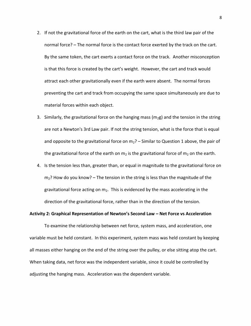
2. If not the gravitational force of the earth on the cart, what is the third law pair of the
normal force? – The normal force is the contact force exerted by the track on the cart.
By the same token, the cart exerts a contact force on the track. Another misconception
is that this force is created by the cart’s weight. However, the cart and track would
attract each other gravitationally even if the earth were absent. The normal forces
preventing the cart and track from occupying the same space simultaneously are due to
material forces within each object.
3. Similarly, the gravitational force on the hanging mass (m2g) and the tension in the string
are not a Newton's 3rd Law pair. If not the string tension, what is the force that is equal
and opposite to the gravitational force on m2? – Similar to Question 1 above, the pair of
the gravitational force of the earth on m2 is the gravitational force of m2 on the earth.
4. Is the tension less than, greater than, or equal in magnitude to the gravitational force on
m2? How do you know? – The tension in the string is less than the magnitude of the
gravitational force acting on m2. This is evidenced by the mass accelerating in the
direction of the gravitational force, rather than in the direction of the tension.
Activity 2: Graphical Representation of Newton’s Second Law – Net Force vs Acceleration
To examine the relationship between net force, system mass, and acceleration, one
variable must be held constant. In this experiment, system mass was held constant by keeping
all masses either hanging on the end of the string over the pulley, or else sitting atop the cart.
When taking data, net force was the independent variable, since it could be controlled by
adjusting the hanging mass. Acceleration was the dependent variable.

9
We positioned the motion detector at the end of the track opposite the pulley. It was
activated using LoggerPro, and the cart was allowed to accelerate toward the pulley. From the
motion detector data, LoggerPro produced a velocity vs. time graph:
Figure 3: System Acceleration from Velocity vs Time
The graph suggests that acceleration was roughly constant as the cart moved along the track
toward the pulley, as expected. The acceleration was determined experimentally, from a linear
fit to the velocity vs time data, to be a = 0.2969 m/s2.
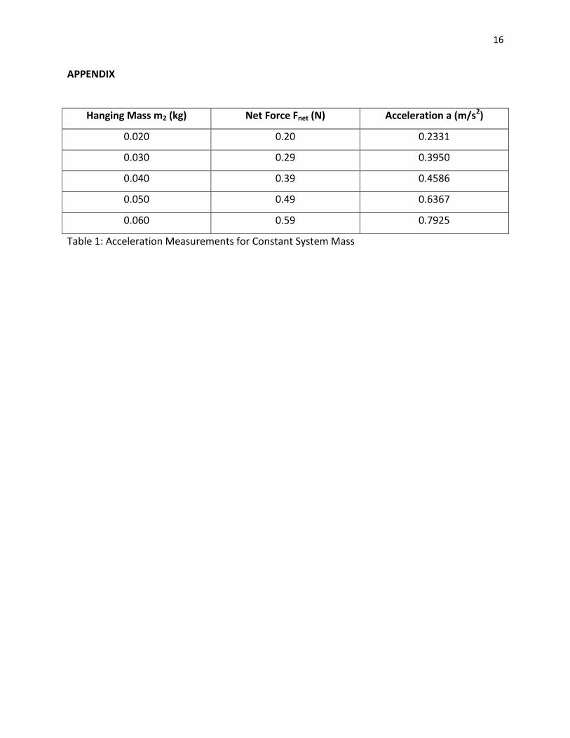
To construct a force vs acceleration graph, the previous procedure was repeated for
various different hanging masses. In each case, an experimental acceleration was obtained
from a linear fit to the velocity vs time graph produced by LoggerPro. The net force acting on
the accelerating system was calculated by multiplying the hanging mass m2 by the acceleration
of gravity g = 9.7953 m/s2. These data are presented in Table 1 in the Appendix.
y = 0.2963x + 0.0005
0
0.5
1
1.5
2
2.5
3
3.5
0 2 4 6 8 10 12
Ve
loci
ty v
(m
/s)
Time t (s)
System Acceleration from Velocity vs Time

10
A graph of net force vs acceleration was created in Microsoft Excel with the data from
Table 1. A linear regression was applied to the graph, giving a graphically-determined value for
the system mass. This graph is displayed in the Results section as Figure 4. Another
experimental value for the system mass was obtained using the double pan balance. After
calibrating it as well as possible, the cart, small masses, and string and paper clips were placed
on one pan. The two 0.200 kg masses were placed on the other pan, as a counterbalance to the
rather heavy cart (the balance can measure 0.110 kg without counterbalance). This measured
system mass is provided in the Results section. It was compared to the graphically-obtained
value using percent difference.
The slope of this graph represents the mass of the accelerating system on the modified
Atwood device. It has units of kilograms, as expected of mass. These units can also be
obtained by interpreting slop as rise over run, or change in y over change in x, and dividing
Netwons (equivalent to kilograms times meters per second squared) by meters per second
squared, leaving kilograms.
11
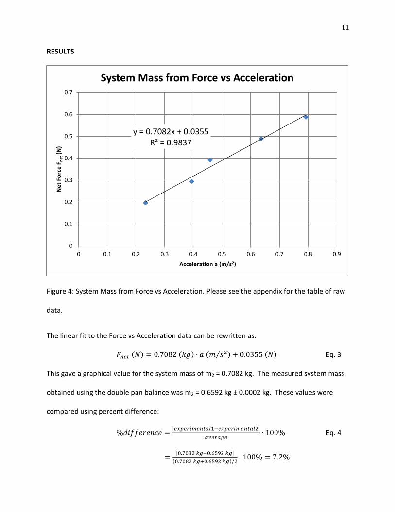
RESULTS
Figure 4: System Mass from Force vs Acceleration. Please see the appendix for the table of raw
data.
The linear fit to the Force vs Acceleration data can be rewritten as:
( ) ( ) ( ⁄ ) ( ) Eq. 3
This gave a graphical value for the system mass of m2 = 0.7082 kg. The measured system mass
obtained using the double pan balance was m2 = 0.6592 kg ± 0.0002 kg. These values were
compared using percent difference:
| |
Eq. 4
| |
( )
y = 0.7082x + 0.0355 R² = 0.9837
0
0.1
0.2
0.3
0.4
0.5
0.6
0.7
0 0.1 0.2 0.3 0.4 0.5 0.6 0.7 0.8 0.9
Ne
t Fo
rce
Fn
et (
N)
Acceleration a (m/s2)
System Mass from Force vs Acceleration
12
DISCUSSION
Data Analysis
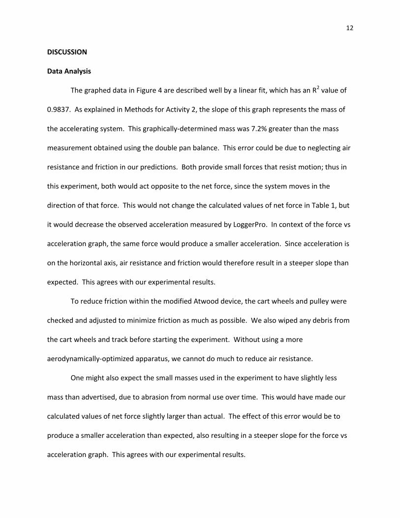
The graphed data in Figure 4 are described well by a linear fit, which has an R2 value of
0.9837. As explained in Methods for Activity 2, the slope of this graph represents the mass of
the accelerating system. This graphically-determined mass was 7.2% greater than the mass
measurement obtained using the double pan balance. This error could be due to neglecting air
resistance and friction in our predictions. Both provide small forces that resist motion; thus in
this experiment, both would act opposite to the net force, since the system moves in the
direction of that force. This would not change the calculated values of net force in Table 1, but
it would decrease the observed acceleration measured by LoggerPro. In context of the force vs
acceleration graph, the same force would produce a smaller acceleration. Since acceleration is
on the horizontal axis, air resistance and friction would therefore result in a steeper slope than
expected. This agrees with our experimental results.
To reduce friction within the modified Atwood device, the cart wheels and pulley were
checked and adjusted to minimize friction as much as possible. We also wiped any debris from
the cart wheels and track before starting the experiment. Without using a more
aerodynamically-optimized apparatus, we cannot do much to reduce air resistance.
One might also expect the small masses used in the experiment to have slightly less
mass than advertised, due to abrasion from normal use over time. This would have made our
calculated values of net force slightly larger than actual. The effect of this error would be to
produce a smaller acceleration than expected, also resulting in a steeper slope for the force vs
acceleration graph. This agrees with our experimental results.

13
The intercept of the force vs acceleration graph was 0.0355, which is reasonably close to
the expected value of zero. The difference could be caused by the entire graph being shifted
vertically by a positive systematic error, or by random errors on each data point.
Another source of error comes from the mass of the string. The string between the cart
and pulley provides a force resisting the motion, while the string between the pulley and
hanging mass adds to the net force acting on the system. The string and paper clips had a mass
of about 3 g, roughly 0.5% of the total system mass, and their effect on the system’s motion
was probably miniscule. However, the variable forces they produce were ignored during the
experiment, and therefore contributed in some way to the error in our results.
Conclusion
We hypothesized that we would be able to determine the system mass graphically, to
within reasonable error, using Newton’s second law in the form of Eq. 2. Our difference of
7.2% supports that hypothesis, but suggests that sources of error were not negligible. As
discussed in the Data Analysis section, air resistance, internal friction, and normal wear on the
small masses used in the experiment would all produce a steeper force vs acceleration graph
than expected. Thus we accept our original hypothesis, with the caveat that these sources of
error were significant, and should somehow be taken into account.
We hypothesized that the vertical intercept of the force vs acceleration graph would be
zero, based on Newton’s first law; in the absence of a net force, an object will not accelerate.
We accept this hypothesis, given that the intercept is close to zero, and taking into account
possible systematic and random errors.

14
We hypothesized that the system mass obtained graphically would be slightly higher
than the measured mass obtained using the double pan balance, due to friction and air
resistance. We accept this hypothesis, based on our graphically-determined system mass being
7.2% greater than our measured system mass. The caveat in this case is that our prediction did
not account for the small masses having slightly less mass than expected.
This experiment allowed us to distinguish between Newton’s laws of motion, by
applying them separately to a physical experiment. Clearly, when the cart is stationary on the
track, there is no net force acting on it, and its acceleration is zero. This verifies Newton’s first
law. And since neither the cart nor track moves the other, Newton’s third law is also verified;
the cart and track act on each other with an equal and opposite contact force. Activity 2
demonstrated Newton’s second law accurately, considering the sources of error discussed in
the Data Analysis section. In that respect, we learned that Newton’s laws can be used to
predict the motion of a system, but also that air resistance and friction cannot always be
neglected.
One improvement to the experiment design that could be performed easily would be to
measure the small masses individually on the double pan balance, to obtain a more precise
value for each. This would minimize error due to wear on the masses.
Using a sleeker apparatus would reduce air resistance. However an easier method of
minimizing the effect of air resistance would be to use a larger system mass, perhaps by placing
the two 0.200 kg masses on the cart for the acceleration trials.
Friction on the pulley axis and cart axles cannot be reduced much, but minor
adjustments can be made to both to minimize friction. The cart wheels and the track can be

15
cleaned before performing the experiment; this would also reduce friction. Alternatively, if the
experiment were performed in a vacuum, air resistance could be neglected with confidence.
16
APPENDIX
Hanging Mass m2 (kg) Net Force Fnet (N) Acceleration a (m/s2)
0.020 0.20 0.2331
0.030 0.29 0.3950
0.040 0.39 0.4586
0.050 0.49 0.6367
0.060 0.59 0.7925
Table 1: Acceleration Measurements for Constant System Mass

17
REFERENCES
“Error Analysis,” Department of Physics and Astronomy, Appalachian State University,
http://physics.appstate.edu/undergraduate-programs/laboratory/resources/error-
analysis, 6 Oct 2014
“Free Fall 2,” Department of Physics and Astronomy, Appalachian State University,
http://physics.appstate.edu/laboratory/quick-guides/free-fall-2, 6 Oct 2014
“Laboratory Report,” Department of Physics and Astronomy, Appalachian State University,
http://physics.appstate.edu/undergraduate-programs/laboratory/resources/laboratory-
report, 6 Oct 2014
“Motion Detector 2,” Department of Physics and Astronomy, Appalachian State University,
http://physics.appstate.edu/sites/physics.appstate.edu/files/motion_detector.pdf, 6 Oct
2014
“Newton’s Laws,” Department of Physics and Astronomy, Appalachian State University,
http://physics.appstate.edu/laboratory/quick-guides/newtons-laws, 6 Oct 2014
“Significant Figures,” Department of Physics and Astronomy, Appalachian State University,
http://physics.appstate.edu/undergraduate-programs/laboratory/resources/significant-
figures, 6 Oct 2014