Sam Helwany, Ph.D., P.E., Ritu Panda, M.S., and Hani Titi ...
127
University of Wisconsin-Milwaukee Department of Civil Engineering and Mechanics January 2011 Sam Helwany, Ph.D., P.E., Ritu Panda, M.S., and Hani Titi, Ph.D., P.E.
Transcript of Sam Helwany, Ph.D., P.E., Ritu Panda, M.S., and Hani Titi ...
University of Wisconsin-Milwaukee Department of Civil Engineering and Mechanics
January 2011
Sam Helwany, Ph.D., P.E., Ritu Panda, M.S., and Hani Titi, Ph.D., P.E.

Technical Report Documentation Page 1. Report No. WHRP 11-01
2. Government Accession
3. Recipient’s Catalog No
4. Title and Subtitle Development of Full Scale Testing of an Alternate Foundation System for Post and Panel Retaining Walls
5. Report Date March 2009 6. Performing Organization Code Wisconsin Highway Research Program
7. Authors Sam Helwany
8. Performing Organization Report
9. Performing Organization Name and Address Department of Civil Engineering and Mechanics University of Wisconsin-Milwaukee
10. Work Unit No. (TRAIS)
11. Contract or Grant No. WisDOT SPR# 0092-07-06
12. Sponsoring Agency Name and Address Wisconsin Department of Transportation Division of Business Services Research Coordination Section 4802 Sheboygan Ave. Rm 104 Madison WI 53707
13. Type of Report and Period Covered
Final Report, 2006-2010 14. Sponsoring Agency Code
15. Supplementary Notes 16. Abstract The alternate post system offers benefits such as ease of construction, reduced construction time, and lower wall costs. While this system seems feasible, there are concerns regarding its performance, in particular the amount of bending in the post and the defection of the wall due to active earth pressures exerted by the retained soil. Other concerns include the potential damage to the plate during driving, control and accuracy of post alignment, and long term issues such as corrosion and soil creep. The objective of this research project is to assess the feasibility of the alternate post system. If the system is deemed feasible, the research team will develop design criteria for the alternate post system based on exposed wall heights, applied soil loads, post dimensions, and parameters of the retained soil and the foundation soil. 17. Key Words
18. Distribution Statement
No restriction. This document is available to the public through the National Technical Information Service 5285 Port Royal Road Springfield VA 22161
19. Security Classif.(of this report) Unclassified
19. Security Classif. (of this page)
Unclassified
20. No. of Pages
21. Price
Form DOT F 1700.7 (8-72) Reproduction of completed page authorized

DISCLAIMER
This research was funded through the Wisconsin Highway Research Program by the
Wisconsin Department of Transportation and the Federal Highway Administration under
Project 0092-07-06. The contents of this report reflect the views of the authors who are
responsible for the facts and accuracy of the data presented herein. The contents do not
necessarily reflect the official views of the Wisconsin Department of Transportation or
the Federal Highway Administration at the time of publication.
This document is disseminated under the sponsorship of the Department of
Transportation in the interest of information exchange. The United States Government
assumes no liability for its contents or use thereof. This report does not constitute a
standard, specification or regulation.
The United States Government does not endorse products or manufacturers. Trade and
manufacturers’ names appear in this report only because they are considered essential to
the object of the document.
ii
EXECUTIVE SUMMARY
The “post and panel” wall is a retaining wall type that has gained a reasonable amount of
usage because it offers advantages under certain conditions. The procedure for the design
of a post and panel wall involves selecting a post spacing, determining the soil and
surcharge loads acting on that post, and then determining the optimum length and
diameter of the post necessary to develop passive soil pressures sufficient to resist those
loads acting on the post. A post and panel wall may be designed either as a cantilever
system or as a tieback system. This type of wall may be used for either conventional
“bottom up” construction or to retain existing facilities by “top down” construction.
Typical post design consists of a steel “H” section set in a column of concrete. The
column of concrete extends from the final ground surface to the computed base elevation
of the post. The steel “H” section extends from the bottom of the concrete to the design
elevation of the top of the wall. Installing wall panels between the exposed sections of
the posts completes construction. The panels are held in place by the flanges of the “H”
sections. The concrete column is usually in the range of 0.6 to 1.2 m (2 to 4 ft) in
diameter.
Several contractors offering an alternate post design have approached WisDOT. They
have proposed eliminating the concrete column and replacing it with a steel plate of the
same width and length as the concrete column. This plate would be welded to the “H”
section and then the composite unit would be driven into the ground to the required plan
base elevation. The remainder of the construction would proceed without change.
iii

The alternate post system offers benefits such as ease of construction, reduced
construction time, and lower wall costs. The objective of this research project is to assess
the feasibility of the alternative system. A design criteria for the alternative system is
developed based on exposed wall heights, applied soil loads, post dimensions, and
parameters of the retained soil and the foundation soil. Full-scale testing of the
alternative system and the conventional pile with concrete pier system are included as
part of this project. The performance of the two systems is compared under otherwise
identical in-situ and loading conditions.
iv

TABLE OF CONTENTS CHAPTER 1 11.1 INTRODUCTION 11.2 PROBLEM STATEMENT 21.3 OBJECTIVE 3 CHAPTER 2 52.1 CURRENT STATE OF KNOWLEDGE--LATERALLY LOADED PILES 52.2 PRELIMINARY ANALYSIS 82.3 MODIFIED DRUCKER-PRAGER/CAP MODEL 132.4 FE RESULTS VERSUS ODOT FIELD TEST RESULTS 182.5 A PRELIMINARY FEASIBILITY STUDY OF THE PROPOSED PILE WITH
PLATE SYSTEM 19 2.5.1 Foundation Soil Type: Sand 19 2.5.2 Foundation Soil Type: Clay 232.6 OTHER ALTERNATIVES 23 2.6.1 Wide Steel Plate System 24 2.6.2 A Steel Plate with Stiffener System 26 2.6.3 Two U-Sections System 27 2.6.4 Tieback System 27 CHAPTER 3 303.1 FIELD TESTS 303.2 FIELD TEST PROCEDURE 30 3.2.1 Test 1: Pile with Plate System 31 3.2.2 Test 2: Pile with Concrete Pier 413.3 COMPARISON: PILE WITH PLATE SYSTEM VERSUS PILE WITH
CONCRETE PIER SYSTEM 51 CHAPTER 4 554.1 FINITE ELEMENT ANALYSIS OF THE PILE WITH PLATE FIELD TEST 554.2 DESIGN CHARTS FOR THE PILE WITH PLATE SYSTEM: COHESIONLESS
SOILS 634.3 PROPOSED DISPLACEMENT-BASED DESIGN METHOD 724.4 DESIGN CHARTS FOR THE PILE WITH PLATE SYSTEM: COHESIVE SOILS 79 REFERENCES 91APPENDIX A
v
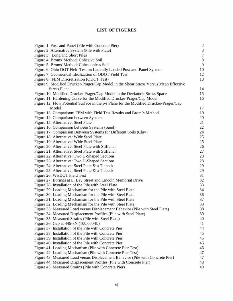
LIST OF FIGURES Figure 1 Post-and-Panel (Pile with Concrete Pier) 2Figure 2 Alternative System (Pile with Plate) 3Figure 3: Long and Short Piles 7Figure 4: Broms' Method: Cohesive Soil 8Figure 5: Broms' Method: Cohesionless Soil 9Figure 6: Ohio DOT Field Test on Laterally Loaded Post-and-Panel System 10Figure 7: Geometrical Idealization of ODOT Field Test 12Figure 8: FEM Discretization (ODOT Test) 13Figure 9: Modified Drucker-Prager/Cap Model in the Shear Stress Versus Mean Effective Stress Plane 14Figure 10: Modified Drucker-Prager/Cap Model in the Deviatoric Stress Space 15Figure 11: Hardening Curve for the Modified Drucker-Prager/Cap Model 16Figure 12: Flow Potential Surface in the p-t Plane for the Modified Drucker-Prager/Cap Model 17Figure 13: Comparison: FEM with Field Test Results and Brom’s Method 19Figure 14: Comparison between Systems 20Figure 15: Alternative: Steel Plate 21Figure 16: Comparison between Systems (Sand) 22Figure 17: Comparison Between Systems for Different Soils (Clay) 24Figure 18: Alternative: Wide Steel Plate 25Figure 19: Alternative: Wide Steel Plate 25Figure 20: Alternative: Steel Plate with Stiffener 26Figure 21: Alternative: Steel Plate with Stiffener 27Figure 22: Alternative: Two U-Shaped Sections 28Figure 23: Alternative: Two U-Shaped Sections 28Figure 24: Alternative: Steel Plate & a Tieback 29Figure 25: Alternative: Steel Plate & a Tieback 29Figure 26: WisDOT Field Test 31Figure 27: Borings at E. Bay Street and Lincoln Memorial Drive 32Figure 28: Installation of the Pile with Steel Plate 33Figure 29: Loading Mechanism for the Pile with Steel Plate 34Figure 30: Loading Mechanism for the Pile with Steel Plate 36Figure 31: Loading Mechanism for the Pile with Steel Plate 37Figure 32: Loading Mechanism for the Pile with Steel Plate 38Figure 33: Measured Load versus Displacement Behavior (Pile with Steel Plate) 38Figure 34: Measured Displacement Profiles (Pile with Steel Plate) 39Figure 35: Measured Strains (Pile with Steel Plate) 40Figure 36: Gap at 445-kN (100,000-lb) 41Figure 37: Installation of the Pile with Concrete Pier 44Figure 38: Installation of the Pile with Concrete Pier 45Figure 39: Installation of the Pile with Concrete Pier 45Figure 40: Installation of the Pile with Concrete Pier 46Figure 41: Loading Mechanism (Pile with Concrete Pier Test) 46Figure 42: Loading Mechanism (Pile with Concrete Pier Test) 47Figure 43: Measured Load versus Displacement Behavior (Pile with Concrete Pier) 47Figure 44: Measured Displacement Profiles (Pile with Concrete Pier) 48Figure 45: Measured Strains (Pile with Concrete Pier) 49
vi

Figure 46: Gap at 556 kN-667 kN (125,000 lb-150,000 lb) 49Figure 47: Cracking at 556 kN-667 kN (125,000 lb-150,000 lb) 50Figure 48: Cracking at 556 kN-667 kN (125,000 lb-150,000 lb) 50Figure 49: Comparison Between Pile with Concrete Pier and Pile with Steel Plate 52Figure 50: Displacement Comparison between Pile with Concrete Pier (Left) and Pile with Steel Plate (Right) 53Figure 51: Strain Comparison between Pile with Concrete Pier (Left) and Pile with Steel Plate (Right) 54Figure 52: Soil Profile (Boring #2) in the Vicinity of the Field Tests 56Figure 53: Assumed Hardening Curve for the Drucker-Prager/Cap Soil Model 58Figure 54: Stress-Strain Curve of Steel Used in the FE Analysis (Elasto-Plastic Model) 58Figure 55: Finite Element Discretization of the Pile with Plate System 59Figure 56: Comparison between Measured and Calculated Lateral Displacement (Pile with Steel Plate) 61Figure 57: Comparison between Measured and Calculated Lateral Displacement Profiles (Pile with Steel Plate) 62Figure 58: Comparison between Measured and Calculated Strains (Pile with Steel Plate) 63Figure 59: Design Criterion 1 for Piles in Cohesionless Soils with Embedded Length L=10 ft 66Figure 60: Design Criterion 2 for Piles in Cohesionless Soils with Embedded Length L=10 ft 67Figure 61: Design Criterion 1 for Piles in Cohesionless Soils with Embedded Length L=20 ft 68Figure 62: Design Criterion 2 for Piles in Cohesionless Soils with Embedded Length L=20 ft 69Figure 63: Design Criterion 1 for Piles in Cohesionless Soils with Embedded Length L=30 ft 70Figure 64: Design Criterion 2 for Piles in Cohesionless Soils with Embedded Length L=30 ft 71 Figure 65: Design Example 1--Pile in Sand 75Figure 66: Design Example 1--Solution 76Figure 67: Design Example 2--Pile in Sand 78Figure 68: Design Criterion 1 for Piles in Cohesive Soils with Embedded Length L=10 ft 82Figure 69: Design Criterion 2 for Piles in Cohesive Soils with Embedded Length L=10 ft 83Figure 70: Design Criterion 1 for Piles in Cohesive Soils with Embedded Length L=20 ft 84Figure 71: Design Criterion 2 for Piles in Cohesive Soils with Embedded Length L=20 ft 85Figure 72: Design Criterion 1 for Piles in Cohesive Soils with Embedded Length L=30 ft 86Figure 73: Design Criterion 2 for Piles in Cohesive Soils with Embedded Length L=30 ft 87Figure 74: Design Example 3--Pile in Clay 90
vii

LIST OF TABLES Table 1: Undrained Soil Properties 13Table 2: Cap Model Parameters for Field Test Analyses 57Table 3: Analysis Matrix for Cohesionless Soils 64Table 4: Cap Model Parameters for Parametric Analyses (Cohesionless Soils) 65Table 5: Analysis Matrix for Cohesive Soils 79Table 6: Cap Model Parameters for Parametric Analyses (Cohesive Soils) 80
viii

ix
ACKNOWLEDGMENTS
The authors wish to acknowledge WisDOT for supporting the Research Project titled:
Development of Full Scale Testing of an Alternate Foundation System for Post and Panel
Retaining Walls. We appreciate the continuing help and support from WisDOT
personnel especially Mr. Robert Arndorfer, and Mr. Jeffery Horsfall, and all the
Geotechnical TOC members. Our appreciation should also be given to the drilling crews
of WisDOT for their field exploration work. Finally, we thank Edward Gillen, Inc. of
Milwaukee for performing the field tests associated with this project.

CHAPTER 1
1.1 INTRODUCTION
The “post and panel” wall is a retaining wall type that has gained a reasonable amount of
usage because it offers advantages under certain conditions. The procedure for the design
of a post and panel wall involves selecting a post spacing, determining the soil and
surcharge loads acting on that post, and then determining the optimum length and
diameter of the post necessary to develop passive soil pressures sufficient to resist those
loads acting on the post. A post and panel wall may be designed either as a cantilever
system or as a tieback system. This type of wall may be used for either conventional
“bottom up” construction or to retain existing facilities by “top down” construction.
Typical post design consists of a steel “H” section set in a column of concrete as shown
in Figure 1. The column of concrete extends from the final ground surface to the
computed base elevation of the post. The steel “H” section extends from the bottom of
the concrete to the design elevation of the top of the wall. Installing wall panels between
the exposed sections of the posts completes construction. The panels are held in place by
the flanges of the “H” sections. The concrete column is usually in the range of 0.6 to 1.2
m (2 to 4 ft) in diameter.
Several contractors offering an alternate post design have approached WisDOT. They
have proposed eliminating the concrete column and replacing it with a steel plate of the
same width and length as the concrete column (Figure 2). This plate would be welded to
the “H” section and then the composite unit would be driven into the ground to the
required plan base elevation. The remainder of the construction would proceed without
change.
1

Figure 1 Post-and-Panel (Pile with Concrete Pier)
1.2 PROBLEM STATEMENT
The alternate post system (termed: “the pile with plate system” henceforth) offers
benefits such as ease of construction, reduced construction time, and lower wall costs.
While this system seems feasible, there are concerns regarding its performance, in
particular the amount of bending in the post and the defection of the wall due to active
earth pressures exerted by the retained soil. Other concerns include the potential damage
2
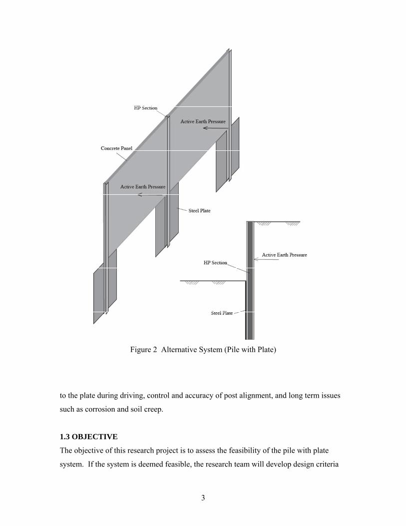
Figure 2 Alternative System (Pile with Plate)
to the plate during driving, control and accuracy of post alignment, and long term issues
such as corrosion and soil creep.
1.3 OBJECTIVE
The objective of this research project is to assess the feasibility of the pile with plate
system. If the system is deemed feasible, the research team will develop design criteria
3

for the pile with plate system based on exposed wall heights, applied soil loads, post
dimensions, and parameters of the retained soil and the foundation soil. Full-scale testing
of the pile with plate system and the conventional pile with concrete pier system will also
be included as part of this project. The performance of the two systems will be compared
under otherwise identical in-situ and loading conditions.
4

CHAPTER 2
2.1 CURRENT STATE OF KNOWLEDGE--LATERALLY LOADED PILES
Fully- and partially-embedded piles and drilled shafts can be subjected to lateral loads, as
well as axial loads, in various applications including sign posts, power poles, marine
pilings, and “post and panel” retaining walls.
Piles and drilled shafts resist lateral loads via shear, bending, and earth passive resistance.
Thus, their resistance to lateral loads depends on (a) pile stiffness and strength: pile
configuration, in particular, the pile length-to-diameter ratio plays an important role in
determining pile stiffness, hence its ability to resist shear and bending moments (b) soil
type, stiffness, and strength, and (c) end conditions: fixed end (due to pile group cap)
versus free end.
Several analytical approaches are available for the design of laterally loaded piles and
drilled shafts. These approaches can be divided into three categories: elastic approach,
ultimate load approach, and numerical approach.
The elastic approach is used to estimate the response of piles subjected to working loads
assuming that the soil and the pile behave as elastic materials. Ultimate loads cannot be
calculated using this “elastic” approach. Matlock and Reese (1960) proposed a method
for calculating moments and displacements along a pile embedded in a cohesionless soil
and subjected to lateral loads and moments at the ground surface. They used a simple
Winkler’s model that substitutes the elastic soil that surrounds the pile with a series of
independent elastic springs. Using the theory of beams on an elastic foundation they
were able to obtain useful equations that allow the calculation of lateral deflections,
slopes, bending moments, and shear forces at any point along the axis of a laterally
loaded pile. A similar elastic solution by Davisson and Gill (1963) is also available for
laterally loaded piles embedded in cohesive soils. Note that this approach requires the
coefficient of subgrade reaction at various depths be known. Best results can be obtained
if this coefficient is measured in the field, but that is rarely done.
5

Several methods that use the ultimate load approach are available for the design of
laterally loaded piles and drilled shafts (example: Broms’ method, 1964; and Meyerhof’s
method, 1995). These methods provide solutions in the form of graphs and tables that are
easy to use by students and engineers.
The ultimate load approach embodied in Broms’ method is suitable for short and long
piles, for restrained- and free-headed piles, and for cohesive and cohesionless soils. A
short pile will rotate as one unit when it is subjected to lateral loads as shown in Figure 3.
The soil in contact with the short pile is assumed to fail in shear when the ultimate lateral
load is reached. On the other hand, a long pile is assumed to fail due to the bending
moments caused by the ultimate lateral load, i.e., the shaft of the pile will fail at the point
of maximum bending moment forming a “plastic hinge” as shown in the same figure.
Broms’ method presents the solution for short piles embedded in cohesive soils with a set
of curves shown in Figure 4a. The curves relate the pile’s embedment length-to-
diameter ratio, L/D, to the normalized ultimate lateral force, Qu/cuD2, for various e/D
ratios. In the figure, the term “restrained-headed” pile indicates that the head of the pile
is connected to a rigid cap that prevents the head of the pile from rotation.
In general, piles having a length-to-diameter ratio (L/D) greater than 20 are long piles.
Figure 4b can be used for long piles embedded in cohesive soils. The curves in this
figure relate the normalized ultimate lateral force, Qu/cuD2, to the normalized yield
moment of the pile, Myield/cuD3, for various e/D ratios. These curves are used only when
L/D>20 and when the moment generated by the ultimate lateral load is greater than the
yield moment of the pile.
For short piles embedded in cohesionless soils, Broms’ method provides the curves given
in Figure 5a that relate the pile’s embedment length-to-diameter ratio, L/D, to the
normalized ultimate lateral force, Qu/KpD3γ, for various e/D ratios. Note that Kp is the
6

passive lateral earth pressure coefficient, and γ is the unit weight of the soil around the
pile.
Figure 3: Long and Short Piles
Figure 5b can be used for long piles embedded in cohesionless soils. The curves in this
figure relate the normalized ultimate lateral force, Qu/KpD3γ, to the normalized yield
moment of the pile, Myield/KpD4γ, for various e/D ratios. These curves are used only
when L/D>20 and when the moment generated by the ultimate lateral load is greater than
the yield moment of the pile.
7

Figure 4: Broms' Method: Cohesive Soil
2.2 PRELIMINARY ANALYSIS
The finite element method is used to investigate the feasibility of the proposed pile with
plate system. Because of the three-dimensional nature of a laterally loaded post system, a
3-D finite element code will be used. The finite element code used herein embodies
advanced soil models capable of simulating drained and undrained loading conditions for
virtually any type of soil and soil strata. It is also capable of simulating the interaction
between the structure (i.e., the post with a concrete column, and the post with a welded
plate) and the soil during lateral loading. The proposed finite element code has been
verified by means of simulating several full-scale lateral load tests on posts with concrete
columns that were performed by Ohio Department of Transportation (ODOT).
Subsequent to code verification, the proposed pile with plate system was analyzed using
8

Figure 5: Broms' Method: Cohesionless Soil
a 25-mm (1-inch) thick plate. The deflections of the post at ground level were compared
with those of the conventional post system as described in a subsequent Section.
A full-scale lateral load test on a post with concrete column performed by Ohio
Department of Transportation (ODOT) will be analyzed herein using the proposed finite
element code. The purpose of this analysis is to show that the proposed finite element
analysis is capable of simulating the behavior of laterally loaded post and panel systems.
The following example describes a post with a concrete column lateral load test that was
carried out by ODOT. Test results will be compared with (a) the Broms’ method
described earlier, and (b) finite element analysis. The concrete column is 3.66-m (12-ft)
9
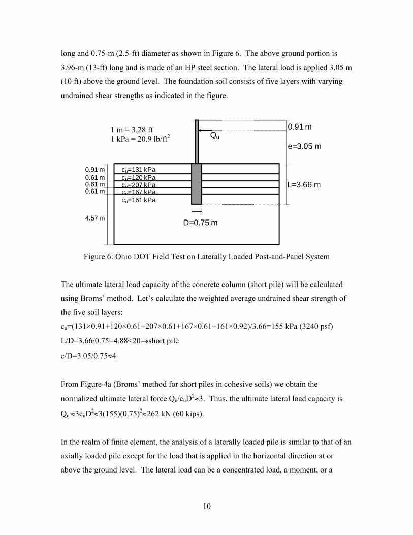
long and 0.75-m (2.5-ft) diameter as shown in Figure 6. The above ground portion is
3.96-m (13-ft) long and is made of an HP steel section. The lateral load is applied 3.05 m
(10 ft) above the ground level. The foundation soil consists of five layers with varying
undrained shear strengths as indicated in the figure.
L=3.66 m
e=3.05 m
0.91 m
D=0.75 m
Qu
0.61 m0.61 m0.91 m
0.61 m
4.57 m
cu=131 kPacu=120 kPacu=207 kPacu=167 kPacu=161 kPa
1 m = 3.28 ft 1 kPa = 20.9 lb/ft2
Figure 6: Ohio DOT Field Test on Laterally Loaded Post-and-Panel System The ultimate lateral load capacity of the concrete column (short pile) will be calculated
using Broms’ method. Let’s calculate the weighted average undrained shear strength of
the five soil layers:
cu=(131×0.91+120×0.61+207×0.61+167×0.61+161×0.92)/3.66=155 kPa (3240 psf)
L/D=3.66/0.75=4.88<20short pile
e/D=3.05/0.754
From Figure 4a (Broms’ method for short piles in cohesive soils) we obtain the
normalized ultimate lateral force Qu/cuD23. Thus, the ultimate lateral load capacity is
Qu 3cuD23(155)(0.75)2262 kN (60 kips).
In the realm of finite element, the analysis of a laterally loaded pile is similar to that of an
axially loaded pile except for the load that is applied in the horizontal direction at or
above the ground level. The lateral load can be a concentrated load, a moment, or a
10

combination of the two. In the case of an axially loaded pile, the finite element mesh of
the pile and the surrounding soil can take advantage of axisymmetry since the geometry
and the loading are both symmetrical about a vertical axis passing through the center of
the pile. This simplification cannot be used for a pile that is loaded with a lateral load,
since the lateral load is applied horizontally in only one direction, i.e., in a non-
symmetrical manner.
Using the finite element method we will calculate the ultimate lateral load capacity of the
post with concrete column system described above. We will assume undrained loading
conditions and then compare the predicted lateral load-displacement curve from the finite
element analysis with the field test results obtained by ODOT.
In this example a limit equilibrium solution is sought for clay strata loaded in an
undrained condition by a single “pile” with a lateral load applied above ground level.
Piles with lateral loads are three-dimensional by nature and will be treated as such in the
following finite element analysis. Note that this problem is symmetrical about a plane
that contains the vertical axis of the pile and the line of action of the lateral load. Thus,
the finite element mesh of half of the pile and half the surrounding soil is considered as
shown in Figures 7 and 8.
Interface elements that are capable of simulating the frictional interaction between the
pile surface and the soil are used. Since this is a non-displacement (bored) pile, the
excess pore water pressure after pile installation is assumed to be zero in this finite
element analysis.
The three-dimensional finite element mesh, shown in Figure 8, comprises two parts: the
concrete pile with the above ground HP section and the soil. The mesh is 30-m (100-ft)
long in the x-direction, 15-m (50-ft) wide in the y-direction, and 7.3-m (25-ft) high in the
z-direction. Mesh dimensions should be chosen in a way that the boundaries do not
affect the solution. This means that the mesh must be extended in all three dimensions,
and that is considered in this mesh.
11
Plane of Symmetry
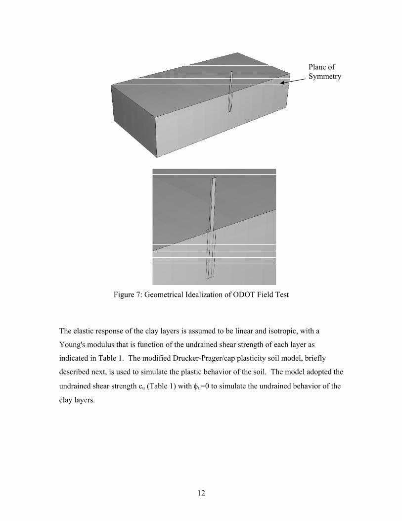
Figure 7: Geometrical Idealization of ODOT Field Test
The elastic response of the clay layers is assumed to be linear and isotropic, with a
Young's modulus that is function of the undrained shear strength of each layer as
indicated in Table 1. The modified Drucker-Prager/cap plasticity soil model, briefly
described next, is used to simulate the plastic behavior of the soil. The model adopted the
undrained shear strength cu (Table 1) with u=0 to simulate the undrained behavior of the
clay layers.
12

Figure 8: FEM Discretization (ODOT Test)
Table 1: Undrained Soil Properties
Soil Layer Depth (m) cu (kPa) E (MPa)
1 (top) 0-0.91 131 32.7
2 0.91-1.52 120 30
3 1.52-2.13 207 51.7
4 2.13-2.74 167 41.9
5 (bottom) 2.74-7.31 161 40.3
1 m=3.28 ft 1 kPa= 20.9 psf
2.3 MODIFIED DRUCKER-PRAGER/CAP MODEL
The Drucker-Prager/Cap plasticity model has been widely used in finite element analysis
programs for a variety of geotechnical engineering applications. The cap model is
appropriate to soil behavior because it is capable of considering the effect of stress
history, stress path, dilatancy, and the effect of the intermediate principal stress.
The yield surface of the modified Drucker-Prager/Cap plasticity model consists of three
parts: a Drucker-Prager shear failure surface, an elliptical “cap,” which intersects the
13

mean effective stress axis at a right angle, and a smooth transition region between the
shear failure surface and the cap as shown in Figure 9.
Figure 9: Modified Drucker-Prager/Cap Model in the Shear Stress Versus Mean
Effective Stress Plane
The elastic behavior is modeled as linear elastic using the generalized Hooke’s law.
Alternatively, an elasticity model in which the bulk elastic stiffness increases as the
material undergoes compression can be used to calculate the elastic strains.
The onset of the plastic behavior is determined by the Drucker-Prager failure surface and
the cap yield surface. The Drucker-Prager failure surface is given by:
0tan dptFs (1)
where is the soil’s angle of friction and d is its cohesion in the p-t plane as indicated in
Figure 9.
14

Figure 10: Modified Drucker-Prager/Cap Model in the Deviatoric Stress Space
As shown in Figure 9, the cap yield surface is an ellipse with eccentricity=R in the p-t
plane. The cap yield surface is dependent on the third stress invariant, r, in the
deviatoric plane as shown in Figure 10. The cap surface hardens (expands) or softens
(shrinks) as a function of the volumetric plastic strain. When the stress state causes
yielding on the cap, volumetric plastic strain (compaction) results causing the cap to
expand (hardening). But when the stress state causes yielding on the Drucker-Prager
shear failure surface, volumetric plastic dilation results causing the cap to shrink
(softening). The cap yield surface is given as:
0)tan(])cos1(
[)( 22
aac pdR
RtppF (2)
where
R is a material parameter that controls the shape of the cap
is a small number (typically 0.01 to 0.05) used to define a smooth transition
surface between the Druker-Prager shear failure surface and the cap:
15
0)tan(]tan)(cos
1([)( 22
aaat pdpdtppF (3)
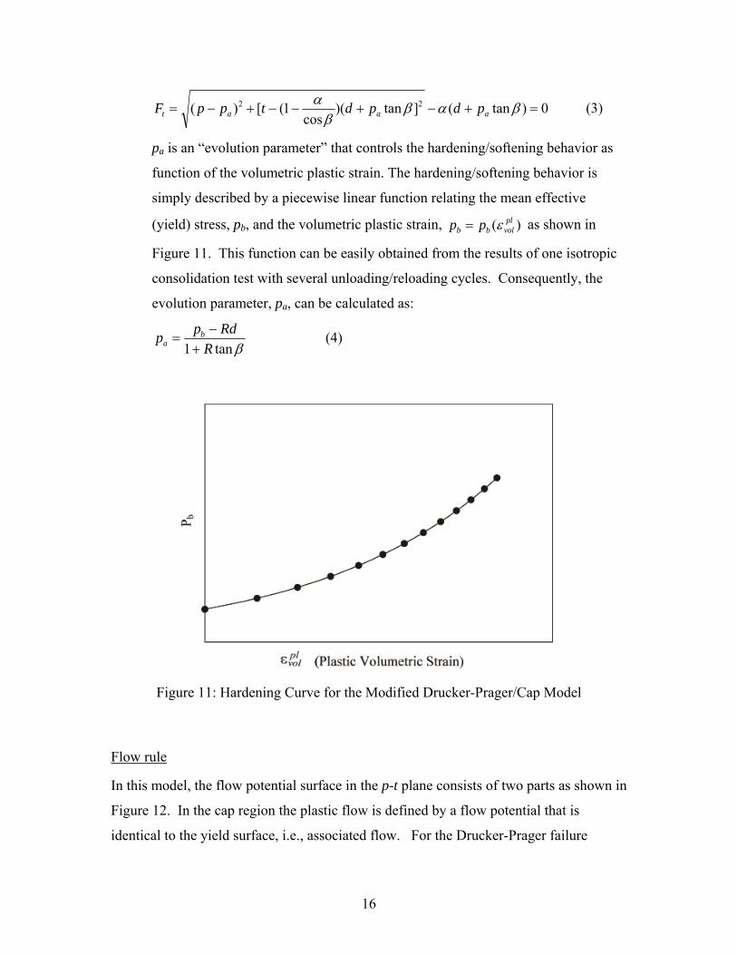
pa is an “evolution parameter” that controls the hardening/softening behavior as
function of the volumetric plastic strain. The hardening/softening behavior is
simply described by a piecewise linear function relating the mean effective
(yield) stress, pb, and the volumetric plastic strain, as shown in
Figure 11. This function can be easily obtained from the results of one isotropic
consolidation test with several unloading/reloading cycles. Consequently, the
evolution parameter, pa, can be calculated as:
)( plvolbb pp
tan1 R
Rdpp b
a
(4)
Figure 11: Hardening Curve for the Modified Drucker-Prager/Cap Model
Flow rule
In this model, the flow potential surface in the p-t plane consists of two parts as shown in
Figure 12. In the cap region the plastic flow is defined by a flow potential that is
identical to the yield surface, i.e., associated flow. For the Drucker-Prager failure
16

surface and the transition yield surface a nonassociated flow is assumed: the shape of the
flow potential in the p-t plane is different from the yield surface shown in Figure 9.
Figure 12: Flow Potential Surface in the p-t Plane for the Modified Drucker-Prager/Cap
Model
In the cap region the elliptical flow potential surface is given as:
22 ])cos1(
[)(
Rt
ppG ac (5)
The elliptical flow potential surface portion in the Drucker-Prager failure and transition
regions is given as:
22 ])cos1(
[]tan)[(
t
ppG as (6)
As shown in Figure 12, the two elliptical portions, Gc and Gs, provide a continuous
potential surface. Because of the nonassociated flow used in this model, the material
stiffness matrix is not symmetric. Thus, an unsymmetric solver should be used in
association with the Cap model.
17
Model Parameters
We need the results of at least three triaxial compression tests to determine the
can be plotted
ear function relating the hydrostatic compression yield stress, pb, and the
orresponding volumetric plastic strain, (Figure 11). The
he volumetric elastic strain that
pile
rtly
reater rate indicating that the lateral load capacity
f the pile has been reached. For comparison, the pile lateral load capacity of 265 kN (60
easured results. Note that the ODOT test included two cycles of
ading and unloading, and that the pile failed at a lateral load of approximately 480 kN
(107 kips). Also, it can be concluded from the figure that the ultimate lateral load of the
parameters d and . The at-failure conditions taken from the tests results
in the p-t plane. A straight line is then best fitted to the three (or more) data points. The
intersection of the line with the t-axis is d and the slope of the line is .
We also need the results of one isotropic consolidation test with several
unloading/reloading cycles. This can be used to evaluate the hardening/softening law as
a piecewise lin
)( plvolbb pp c
unloading/reloading slope can be used to calculate t
should be subtracted from the volumetric total strain in order to calculate the volumetric
plastic strain.
2.4 FE Results versus ODOT Field Test Results
The pile lateral load capacity versus displacement curve obtained from the finite element
analysis is shown in Figure 13. It is noted from the figure that the horizontal
displacement increases as the lateral load is increased up to about 475-kN (106 kips)
load at which a horizontal displacement of about 5 cm (2 inch) is encountered. Sho
after that, the pile moves laterally at a g
o
kips), predicted by Broms’ Method, is shown in Figure 13. It is noted that the finite
element prediction of pile lateral load capacity is about two times greater than the
capacity predicted by Broms’ method.
More importantly, Figure 13 provides the load-displacement curve obtained from the
field test conducted on the same pile by ODOT. The finite element results are in good
agreement with the m
lo
18

pile predicted by Broms’ method seriously underestimated the measured lateral load
capacity of the pile.
Figure 13: Comparison: FEM with Field Test Results and Brom’s Method
2.5 A PRELIMINARY FEASIBILITY STUDY OF THE PROPOSED PILE WITH
PLATE SYSTEM
2.5.1 Foundation Soil Type: Sand
The research team carried out a preliminary feasibility analysis of the proposed pile w
plate system using the finite element code that has been verified as described in the
previous Section. The preliminary feasibility analysis consisted of an objective
comparison of the behavior of a conventi
ith
onal post with a concrete column and a post
ith a welded plate. The two post systems analyzed herein are identical to the proposed
post systems for the field test (Figure 14). This preliminary feasibility analysis will shed
some light on the proposed post system.
1 cm = 0.39 inch 1 kN = 0.225 kips
w
19
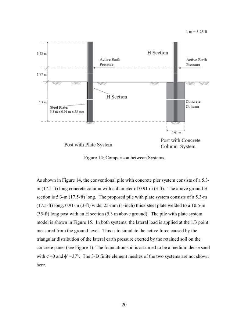
Figure 14: Comparison between Systems
As shown in Figure 14, the conventional pile with concrete pier system consists of a 5.3-
m (17.5-ft) long concrete column with a diameter of 0.91 m (3 ft). The above ground H
section is 5.3-m (17.5-ft) long. The proposed pile with plate system consists of a 5.3-m
(17.5-ft) long, 0.91-m (3-ft) wide, 25-mm (1-inch) thick steel plate welded to a 10.6-m
(35-ft) long post with an H section (5.3 m above ground). The pile with plate system
model is shown in Figure 15. In both systems, the lateral load is applied at the 1/3 point
measured from the ground level. This is to simulate the active force caused by the
triangular distribution of the lateral earth pressure exerted by the retained soil on the
concrete panel (see Figure 1). The foundation soil is assumed to be a medium dense sand
with c=0 and =37. The 3-D finite element meshes of the two systems are not shown
here.
20

1 inch = 2.54 cm 1 ft = 0.3048 m
Figure 15: Alternative: Steel Plate
Figure 16 shows the predicted horizontal displacement versus applied lateral load for
both post systems. In the figure, the horizontal displacement is the displacement of the
post at the ground level. It is clear from the figure that the conventional post with
concrete column system is much stiffer than the proposed pile with plate system. For a
5.3 m (17.5-ft) high concrete panel spanning 3 m (10 ft) between two posts, center to
center, the active lateral force exerted on the concrete panel is approximately 200 kN (45
kips). From Figure 16 this lateral load will cause a horizontal displacement of 4 mm
(0.16 inch) in the conventional post with concrete column system. In contrast, the same
load will cause 25 mm (1 inch) of horizontal displacement in the proposed pile with plate
system. This large difference in displacement is attributed to the large flexural stiffness
of the concrete column in the conventional post system as compared to the flexural
stiffness of the 25-mm (1-inch) thick steel plate in the proposed pile with plate system.
Using typical values of Young’s moduli for steel and concrete we can calculate the
stiffness of the concrete column as:
21

ftlbL
rE
L
IE
column
concrete
column
columnconcrete .103.1365.17
)5.1(4
1100.6
4
1
6
484
And the stiffness of the steel plate is:
ftlbL
tbE
L
IE
plate
steel
plate
platesteel .10036.05.17
)12
1(
12
3103.412 6
39
3
This means that the stiffness of the concrete column is approximately 3800 times greater
than the stiffness of the steel plate for this specific example.
1 mm = 0.04 inch 1 kN = 0.225 kips
Figure 16: Comparison between Systems (Sand)
A question arises now, is 25 mm (1 inch) of horizontal displacement tolerable for the
proposed pile with plate system under a working load of 200 kN (45 kips)? If the answer
is NO then the proposed system needs to be improved. In such case, one can increase the
stiffness of the plate and the stiffness of the post (H section). Note that this discussion is
22

only based on a single case, and many other cases need to be considered before offering
remedies for the proposed system. Nevertheless, if more stiffness is needed, one can
increase the thickness, and possibly the width, of the plate. Also, plate “stiffeners” can
be used for added stiffness (stiffeners are welded steel sheets that are orthogonal to the
plate). Anchors can also be used to reduce lateral displacements. The embedded length
of the post and the welded plate can be increased as another option. Some of these
options are investigated in the next Section.
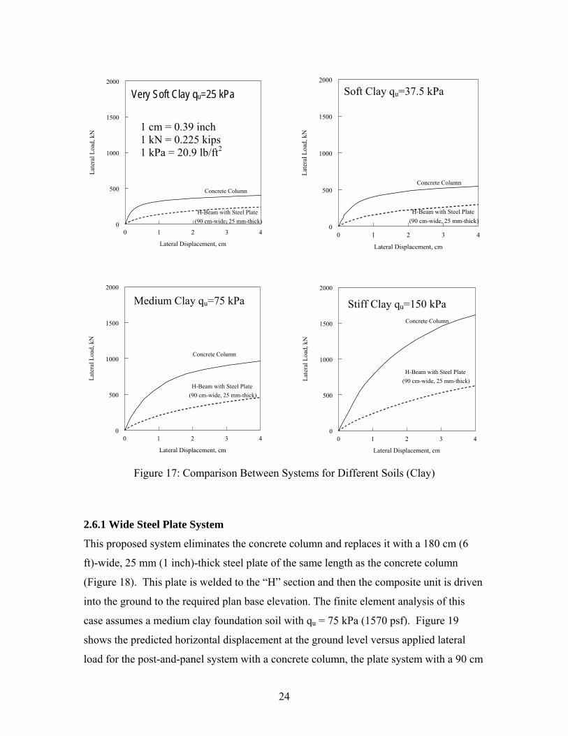
2.5.2 Foundation Soil Type: Clay
The analyses described above was repeated herein four times using the same finite
element mesh and the same parameters except for the foundation soil that is replaced by
four different clayey soils having unconfined compressive strengths qu = 25 kPa (520 psf;
very soft clay), 37.5 kPa (780 psf; soft clay ), 75 kPa (1570 psf; medium clay), and 150
kPa (3130 psf; stiff clay). Figure 17 shows the predicted horizontal displacement (at
ground level) versus applied lateral load for both post systems for the four foundation soil
types. It is clear from the figure that the conventional post with concrete column system
is much stiffer than the proposed pile with plate system. As was done in the previous
Section, Figure 17 can be used to estimate the horizontal displacement of the post at the
ground level under the action of horizontal loads caused by active earth pressures.
2.6 OTHER ALTERNATIVES
The finite element analysis is extended to include four other possible systems that may be
used to replace or enhance the proposed pile with plate system. These are: (1) a wide
steel plate system, (2) a steel plate with stiffener system, (3) a two U-sections system, and
(4) a tieback system.
23
0
500
1000
1500
2000
Lat
eral
Loa
d, k
N
0
500
1000
1500
2000
Lat
eral
Loa
d, k
N
Figure 17: Comparison Between Systems for Different Soils (Clay)
2.6.1 Wide Steel Plate System
This proposed system eliminates the concrete column and replaces it with a 180 cm (6
ft)-wide, 25 mm (1 inch)-thick steel plate of the same length as the concrete column
(Figure 18). This plate is welded to the “H” section and then the composite unit is driven
into the ground to the required plan base elevation. The finite element analysis of this
case assumes a medium clay foundation soil with qu = 75 kPa (1570 psf). Figure 19
shows the predicted horizontal displacement at the ground level versus applied lateral
load for the post-and-panel system with a concrete column, the plate system with a 90 cm
0 1 2 3 4
Lateral Displacement, cm
Concrete Column
H-Beam with Steel Plate
(90 cm-wide, 25 mm-thick)
0 1 2 3 4
Lateral Displacement, cm
Concrete Column
H-Beam with Steel Plate
(90 cm-wide, 25 mm-thick)
0 1 2 3 4
Lateral Displacement, cm
0
500
1000
1500
2000
Lat
eral
Loa
d, k
N
Concrete Column
H-Beam with Steel Plate
(90 cm-wide, 25 mm-thick)
0 1 2 3 4
Lateral Displacement, cm
0
500
1000
1500
2000
Lat
eral
Loa
d, k
N
Concrete Column
H-Beam with Steel Plate
(90 cm-wide, 25 mm-thick)
Pa Soft Clay qu=37.5 kPa Very Soft Clay qu=25 k
1 cm = 0.39 inch 1 kN = 0.225 kips 1 kPa = 20.9 lb/ft2
Medium Clay qu=75 kPa Stiff Clay qu=150 kPa
24

(3 ft)-wide steel plate, and the plate system with a 180 cm (6 ft)-wide steel plate. The
figure clearly indicates that the wider steel plate system offers a slight improvement to
the 90 cm (3 ft)-wide steel plate (i.e., the wider plate is not warranted).
1 inch = 2.54 cm 1 ft = 0.3048 m
Figure 18: Alternative: Wide Steel Plate
0 1 2 3
Lateral Displacement, cm
40
500
1000
1500
2000
Lat
eral
Loa
d, k
N
Concrete Column
Steel Plate (90 cm-wide)
Steel Plate (180 cm-wide)
1 cm = 0.39 inch 1 kN = 0.225 kips
Figure 19: Alternative: Wide Steel Plate
25

2.6.2 A Steel Plate with Stiffener System
This system, shown in Figure 20, consists of a 90 cm (3 ft)-wide, 25 mm (1 inch)-thick
steel plate that is welded to the H-beam, and a stiffener plate, 30 cm (1 ft)-wide and 25
mm (1 inch)-thick, that is orthogonally welded to the 90 cm (3 ft)-wide plate as shown in
the figure. As in the previous analysis the finite element analysis of this case assumes a
medium clay foundation soil with qu = 75 kPa (1570 psf). Figure 21 shows the predicted
horizontal displacement at the ground level versus applied lateral load for the post-and-
panel system with a concrete column, the plate system with a 90 cm (3 ft)-wide steel
plate, and the plate system with a stiffener. Again, the figure indicates that the steel plate
with stiffener system offers some improvement to the 90 cm (3 ft)-wide steel plate. More
improvement can be attained by increasing the width of the stiffener.
1 inch = 2.54 cm 1 ft = 0.3048 m
Figure 20: Alternative: Steel Plate with Stiffener
26

0 1 2 3
Lateral Displacement, cm
40
500
1000
1500
2000
Lat
eral
Loa
d, k
NConcrete Column
Steel Plate without Stiffener
Steel Plate with Stiffener
1 cm = 0.39 inch 1 kN = 0.225 kips
Figure 21: Alternative: Steel Plate with Stiffener
2.6.3 Two U-Sections System
Figure 22 illustrates this system that consists of two channel sections welded to the H-
beam. The channel section used in this analysis is 30 cm (1 ft)-wide, 30 cm (1 ft)-deep,
and 25 mm (1 inch)-thick. As in the previous analysis the finite element analysis of this
case assumes a medium clay foundation soil with qu = 75 kPa (1570 psf). Figure 23
shows the predicted horizontal displacement at the ground level versus applied lateral
load for the post-and-panel system with a concrete column, the plate system with a 90 cm
(3 ft)-wide steel plate, and the two U-sections system. The figure shows that the two U-
sections system offers a slight improvement to the 90 cm (3 ft)-wide steel plate at early
stages of loading. At loads greater than approximately 250 kN (56 kips) this
improvement diminishes as shown in the figure.
2.6.4 Tieback System
This proposed system consists of a 90 cm (3 ft)-wide, 25 mm (1 inch)-thick steel plate of
the same length as the concrete column (Figure 24). A tieback system consisting of a
27

1 inch = 2.54 cm 1 ft = 0.3048 m
Figure 22: Alternative: Two U-Shaped Sections
1 cm = 0.39 inch 1 kN = 0.225 kips
Figure 23: Alternative: Two U-Shaped Sections
steel cable attached to the H-beam 30 cm (1 ft) below the ground level at one end, and to
a concrete block at the other end. The cable is attached to the H-Beam after the
composite unit (H-beam and the welded steel plate) is driven into the ground to the
28
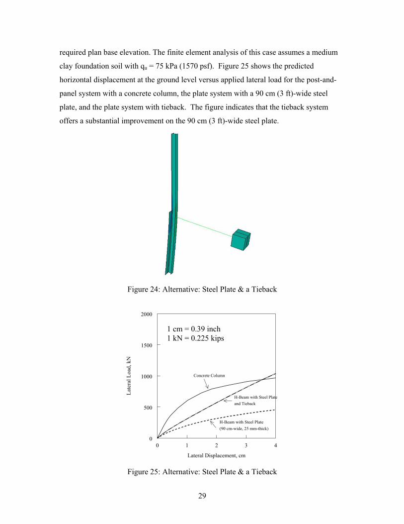
required plan base elevation. The finite element analysis of this case assumes a medium
clay foundation soil with qu = 75 kPa (1570 psf). Figure 25 shows the predicted
horizontal displacement at the ground level versus applied lateral load for the post-and-
panel system with a concrete column, the plate system with a 90 cm (3 ft)-wide steel
plate, and the plate system with tieback. The figure indicates that the tieback system
offers a substantial improvement on the 90 cm (3 ft)-wide steel plate.
Figure 24: Alternative: Steel Plate & a Tieback
0 1 2 3
Lateral Displacement, cm
40
500
1000
1500
2000
Lat
eral
Loa
d, k
N
Concrete Column
H-Beam with Steel Plate
(90 cm-wide, 25 mm-thick)
H-Beam with Steel Plate
and Tieback
1 cm = 0.39 inch 1 kN = 0.225 kips
Figure 25: Alternative: Steel Plate & a Tieback
29

CHAPTER 3
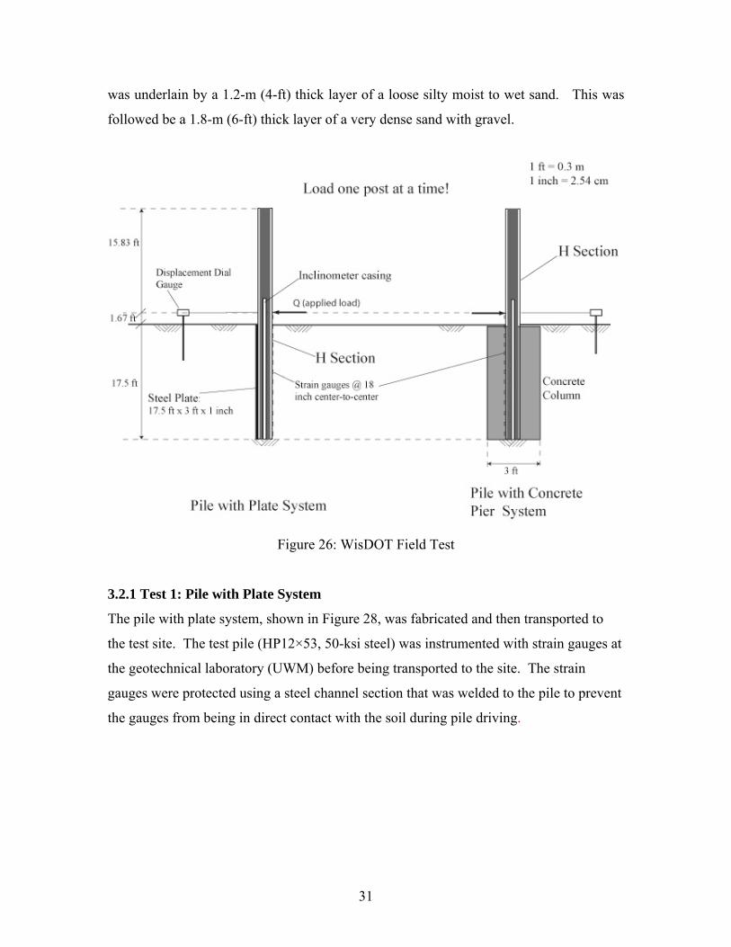
3.1 FIELD TESTS
Two full-scale field tests were performed to investigate the performance of the proposed
pile with plate system. The configuration of the field tests and instrumentation is shown
in Figure 26. To obtain representative results, the length of the posts below ground level
will be 5.3 m (17.5 ft). The two posts will then be loaded laterally until failure. Each
post will be loaded independently, as opposed to loading one post against the other post.
This is because there is a possibility that one post will fail first, thus the test has to be
terminated prematurely before loading the second post to failure.
Both post systems were instrumented to determine their response to lateral loading,
especially longitudinal strains and lateral deflections. The instrumentation program
included inclinometers to determine lateral displacement profiles of the post in both
systems. It also included strain gauges along the post of both systems to determine strain
distribution. The lateral load was applied in small increments (approximately 10% of the
estimated failure load). All deflection and strain measurements were taken immediately
after the load increment was applied.
3.2 FIELD TEST PROCEDURE
Full-scale testing of the pile with plate system and the conventional pile with concrete
pier system were performed as part of this project. The performance of the two systems
is compared under otherwise nearly identical in-situ and loading conditions. The tests
were performed at a site near the intersection of E. Bay Street and Lincoln Memorial
Drive in Milwaukee (site belongs to the Port Authority). An aerial photo of the site is
shown in Figure 27. Note the locations of borings 1 and 2 in the figure. Appendix A
provides the details of the two borings. The field tests were performed in the near
vicinity of boring No. 2. Of most interest is the top part of the soil since the embedded
length of the test piles was 5.3 m (17.5 ft). The upper 4.3 m (14 ft) of the soil strata
consisted of a dense to loose granular fill material with fine to coarse sand and gravel.
This soil layer was dry in the most part except for a moist zone at the bottom. This layer
30
was underlain by a 1.2-m (4-ft) thick layer of a loose silty moist to wet sand. This was
followed be a 1.8-m (6-ft) thick layer of a very dense sand with gravel.
Figure 26: WisDOT Field Test
3.2.1 Test 1: Pile with Plate System
The pile with plate system, shown in Figure 28, was fabricated and then transported to
the test site. The test pile (HP12×53, 50-ksi steel) was instrumented with strain gauges at
the geotechnical laboratory (UWM) before being transported to the site. The strain
gauges were protected using a steel channel section that was welded to the pile to prevent
the gauges from being in direct contact with the soil during pile driving.
31
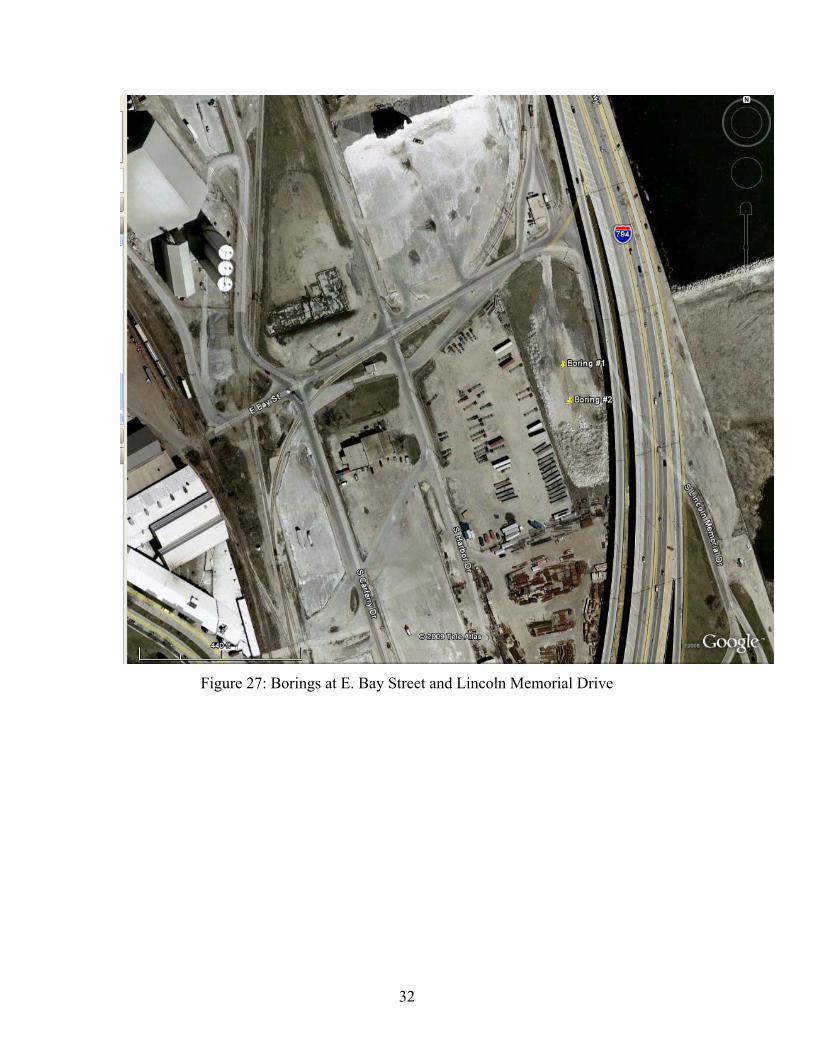
Figure 27: Borings at E. Bay Street and Lincoln Memorial Drive
32

Figure 28: Installation of the Pile with Steel Plate
The horizontal deflections of the pile were measured using an inclinometer as indicated
in Figure 29. The inclinometer flexible casing was protected using a welded steel sleeve
as shown in the same figure. The small space between the protective sleeve and the
inclinometer casing was filled with grout. Inclinometer measurements were taken after
each load increment application.
33

Figure 29: Loading Mechanism for the Pile with Steel Plate
Axial strains in the pile (H beam) were measured using 13 strain gauges. The gauges
were spaced at 45 cm (18 inch) intervals center-to-center as shown in Figure 26. The top
gauge is 45 cm (18 inch) above the ground level, i.e., 5 cm (2 inch) below the point of
load application. Strain gauge readings were taken after the application of each load
increment.
The horizontal deflection of the pile at the point of load application was measured using a
displacement dial gauge mounted on a steel frame supported by four mini piles located
sufficiently away from the test pile to ensure that the supporting frame is unaffected by
ground subsidence associated with pile deflection during testing.
The following is a step-by-step description of the first test:
1. A 2.54-cm thick (1-inch), 0.91-m wide (3-ft), 5.3-m long (17.5-ft) steel plate was
welded to the 10.7-m long (35-ft) H-beam (HP12×53) to form the proposed pile
with plate system. Strain gauges and inclinometer protective sleeve were installed
as shown in Figure 26.
34

2. The proposed plate system was driven to a depth of 5.4 m (17.5 ft) using a
pneumatic hammer (Figure 28). Precautions were exercised to make sure that the
pile with plate system was perfectly vertical upon driving. The actual driving of
the pile was done in a few minutes.
3. Inclinometer casings were inserted inside the inclinometer protective sleeve and
the space in between was grouted (see Figure 29).
4. A loading fixture with a centric hole was welded to the pile. The height of the
center of the hole was 50 cm (20 inch) above ground level (see Figure 29). A
2.54-cm (1-inch) diameter steel bar was used to apply the horizontal load as
shown in the same figure. A crane weighing approximately 890 kN (200,0000 lb)
was situated near the pile (Figure 30) and used as a reaction mass against which a
hydraulic actuator was mounted as shown in Figures 31 and 32.
5. The lateral load on the pile with plate system was increased gradually: 22.25 kN
(5,000 lb), 44.5 kN (10,000 lb), 66.75 kN (15,000 lb), 111.25 kN (25,000 lb),
200.25 kN (45,000 lb), 289.25 kN (65,000 lb), 378.25 kN (85,000 lb), and 445 kN
(100,000 lb). All data were collected at the conclusion of each load increment.
Figure 33 shows the measured horizontal displacements of the pile (at the point of load
application) versus applied load. The figure indicates an approximately linear load-
displacement behavior. At approximately 445-kN (100,000-lb) applied load, the
measured lateral displacement was 3.3 cm (1.3 inch). It is to be noted that at an applied
load of about 445-kN (100,000-lb), the crane that was used as a reaction mass started to
slide. At that instance it was difficult to sustain the load. Nonetheless, a consequent
finite element analysis of the pile with plate test indicated that the A36 steel H pile started
to yield (initial yield) at approximately 445-kN (100,000-lb) applied lateral load.
35
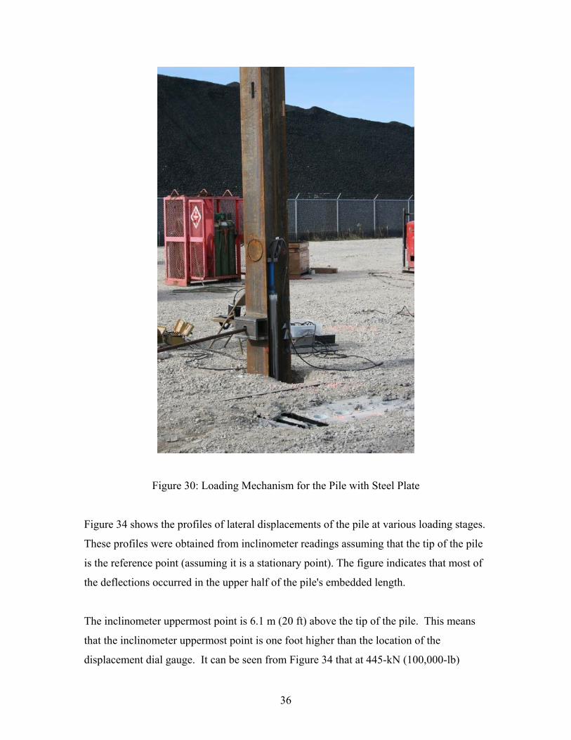
Figure 30: Loading Mechanism for the Pile with Steel Plate
Figure 34 shows the profiles of lateral displacements of the pile at various loading stages.
These profiles were obtained from inclinometer readings assuming that the tip of the pile
is the reference point (assuming it is a stationary point). The figure indicates that most of
the deflections occurred in the upper half of the pile's embedded length.
The inclinometer uppermost point is 6.1 m (20 ft) above the tip of the pile. This means
that the inclinometer uppermost point is one foot higher than the location of the
displacement dial gauge. It can be seen from Figure 34 that at 445-kN (100,000-lb)
36

lateral load, the displacement at the elevation of the displacement gauge (one foot below
the top point of the inclinometer) is approximately 3.3 cm (1.3 inch). This displacement
is the same as that obtained from the displacement dial gauge at the same load (see Figure
33). This shows that the inclinometer displacements in reference to the pile tip are
reasonably accurate, and that the reference point (tip of the pile) was indeed stationary
throughout the load test.
Figure 31: Loading Mechanism for the Pile with Steel Plate
Figure 35 shows the measured axial strains in the pile at various loading stages. It is
noted from the figure that the strain at the tip of the pile and at the point of load
application was always zero. The maximum measured strain at 445-kN (100,000-lb)
lateral load was approximately 1,300 Micro strain and located about 127 cm (50 inch)
below the point of load application. This strain can be well within the yield strain range
for A36 steel (note that the yield strain and yield stress can vary widely for the same type
of steel).
37

Finally, Figure 36 shows a substantial gap between the soil and the back of the pile at
failure load. This gap started with the first lateral load increment and increased gradually
as the lateral load was increased.
Figure 32: Loading Mechanism for the Pile with Steel Plate
1 inch = 2.54 cm 1000 lb=4.448 kN
Figure 33: Measured Load versus Displacement Behavior (Pile with Steel Plate)
38

1 inch = 2.54 cm 1 ft = 0.3048 m 1000 lb=4.448 kN
Figure 34: Measured Displacement Profiles (Pile with Steel Plate)
39

1 inch = 2.54 cm 1 kips = 4.448 kN
Figure 35: Measured Strains (Pile with Steel Plate)
40
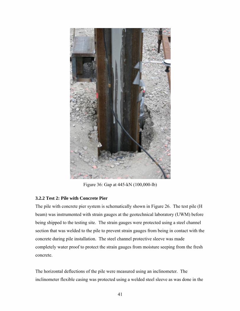
Figure 36: Gap at 445-kN (100,000-lb)
3.2.2 Test 2: Pile with Concrete Pier
The pile with concrete pier system is schematically shown in Figure 26. The test pile (H
beam) was instrumented with strain gauges at the geotechnical laboratory (UWM) before
being shipped to the testing site. The strain gauges were protected using a steel channel
section that was welded to the pile to prevent strain gauges from being in contact with the
concrete during pile installation. The steel channel protective sleeve was made
completely water proof to protect the strain gauges from moisture seeping from the fresh
concrete.
The horizontal deflections of the pile were measured using an inclinometer. The
inclinometer flexible casing was protected using a welded steel sleeve as was done in the
41

first test. The small space between the protective sleeve and the inclinometer casing was
filled with grout. Inclinometer measurements were taken after each load increment
application.
Axial strains in the pile (H beam) were measured using 13 strain gauges. The gauges
were spaced at 45.7 cm (18 inch) intervals center-to-center as shown in Figure 26. The
top gauge is 45.7 cm (18 inch) above the ground level, i.e., 5 cm (2 inch) below the point
of load application. Strain gauge readings were taken after the application of each load
increment.
The horizontal deflection of the pile at the point of load application was measured using a
displacement dial gauge mounted on a steel frame supported by four mini piles located
sufficiently away from the test pile to ensure that the supporting frame is unaffected by
ground subsidence associated with pile deflection during testing.
The following is a step-by-step description of the second test:
1. A 5.3-m (17.5-ft) deep, 0.91-m (3-ft) diameter hole was drilled as shown in
Figures 37 and 38. There was no need to support the excavation during
construction.
2. A 10.7-m (35-ft) long H-beam (HP12×53) was positioned at the center of the hole
(Figure 39).
3. Concrete was poured up to ground level as shown in Figures 39 and 40. The
concrete was left to harden for 28 days.
4. Inclinometer casings were installed inside the inclinometer protective sleeve and
the space in between was grouted.
5. A loading fixture with a centric hole was welded to the pile. The height of the
center of the hole was 51 cm (20 inch) above ground level. A 2.54 cm (1-inch)
diameter steel bar was used to apply the horizontal load. A crane weighing
approximately 889 kN (200,0000 lb) was situated near the pile (Figure 41) and
used as a reaction mass against which a hydraulic actuator was mounted. For
42
6. The lateral load on the pile with concrete pier system was increased gradually:
22.25 kN (5,000 lb), 111.25 kN (25,000 lb), 155.75 kN (45,000 lb), 289.25 kN
(65,000 lb), 378.25 kN (85,000 lb), 445 kN (100,000 lb), 556.25 kN (125,000 lb),
and 667.5 kN (150,000 lb) at which failure was deemed imminent. All data were
collected at the conclusion of each load increment.
Figure 43 shows the measured horizontal displacements of the pile (at the point of load
application) versus applied load. A highly nonlinear load-displacement behavior is noted
in the figure. At approximately 667-kN (150,000-lb) applied load, the measured lateral
displacement was 2.54 cm (1.0 inch). Failure was deemed imminent because of the
difficulties encountered trying to maintain the hydraulic pressure in the hydraulic jack at
this load level.
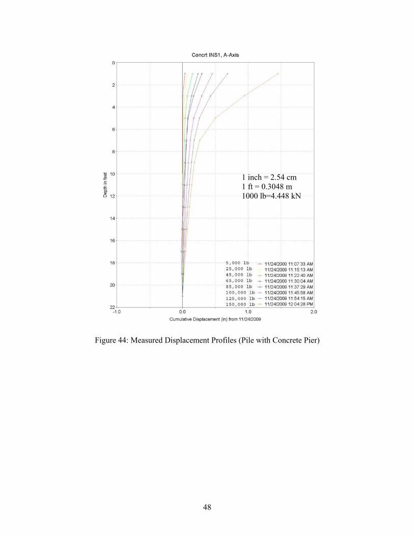
Figure 44 shows the deflection profiles of the pile at various loading stages. These
profiles were obtained from inclinometer readings assuming that the pile tip is the
reference point. The figure shows that the deflections occurred in the entire embedded
length of the pile indicating some rotational tendency.
The inclinometer uppermost point is 6.1 m (20 ft) above the tip of the pile, i.e., one foot
higher than the location of the displacement dial gauge. It can be seen from Figure 44
that at 667-kN (150,000-lb) lateral load, the displacement at the elevation of the
displacement gauge (one foot below the top point of the inclinometer) is approximately 3
cm (1.2 inch). This displacement is slightly larger than that obtained from the
displacement dial gauge at the same load (see Figure 43).
Figure 45 shows the measured axial strains in the pile at various loading stages. It is
noted from the figure that the strains are mostly mobilized in the upper half of the
embedded length of the pile. The maximum measured strain at 667-kN (150,000-lb)
lateral load was approximately 1,400 Micro strain and located about 102 cm (40 inch)
43

below the point of load application. As indicated earlier, this strain can be well within
the yield strain range for A36 steel (note that the yield strain and yield stress can vary
widely for the same type of steel).
Figure 46 shows a gap between the soil and the back of the pier at failure load. This gap
started with the first lateral load increment and increased gradually as the lateral load was
increased. Figures 47 and 48 show minor cracks that appeared in the plain concrete at
higher loads approaching the failure.
Figure 37: Installation of the Pile with Concrete Pier
44

Figure 38: Installation of the Pile with Concrete Pier
Figure 39: Installation of the Pile with Concrete Pier
45

Figure 40: Installation of the Pile with Concrete Pier
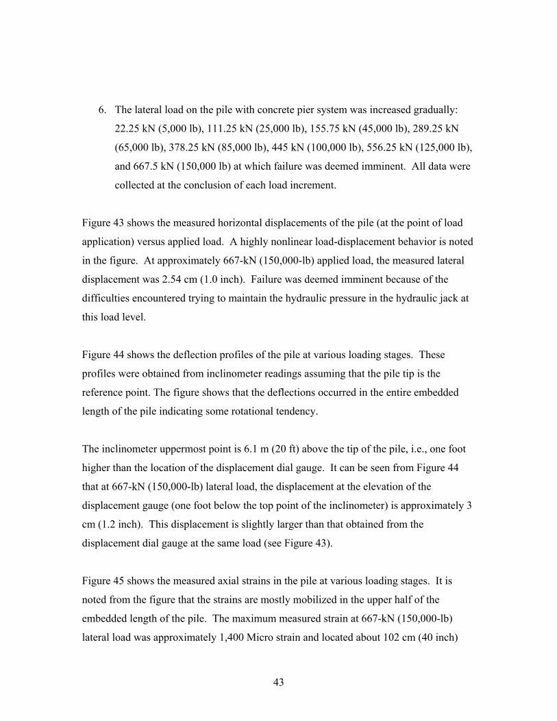
Figure 41: Loading Mechanism (Pile with Concrete Pier Test)
46
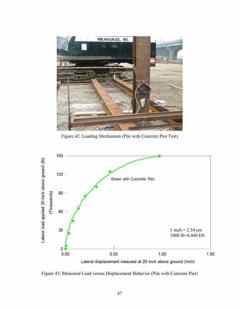
Figure 42: Loading Mechanism (Pile with Concrete Pier Test)
1 inch = 2.54 cm 1000 lb=4.448 kN
Figure 43: Measured Load versus Displacement Behavior (Pile with Concrete Pier)
47
1 inch = 2.54 cm 1 ft = 0.3048 m 1000 lb=4.448 kN
Figure 44: Measured Displacement Profiles (Pile with Concrete Pier)
48

1 inch = 2.54 cm 1 kips = 4.448 kN
Figure 45: Measured Strains (Pile with Concrete Pier)
Figure 46: Gap at 556 kN-667 kN (125,000 lb-150,000 lb)
49

Figure 47: Cracking at 556 kN-667 kN (125,000 lb-150,000 lb)
Figure 48: Cracking at 556 kN-667 kN (125,000 lb-150,000 lb)
50

3.3 COMPARISON: PILE WITH PLATE SYSTEM VERSUS PILE WITH
CONCRETE PIER SYSTEM
The field tests have shown that the pile with plate system offered several benefits such as
ease of construction, reduced construction time, and lower wall costs. The fabrication of
the pile with plate is fairly simple and involved welding the plate to the H beam. To
further save cost one can select a plate with a standard 1.22-m (4-ft) width and use it as
is (without the need for cutting). The installation of the pile with plate system was very
accurate and speedy in this particular soil strata. In this particular field test, the initial
alignment of the system took about five minutes. The actual driving time of the 5.3 m
(17.5 ft) embedded length was 2-3 minutes in a relatively dense granular soil. There was
no apparent damage to the plate during driving (please see video clip of the field test).
Further field tests in difficult soils, such as dense gravely soils, may be needed to
illustrate the applicability of the pile with plate system in terms of installation speed and
alignment control.
The pile with plate system does not require excavation and concrete mixing equipment
and their associated costs, making it a very cost-effective method. The ease of
fabrication and installation in any type of weather makes this system a very attractive
alternative. For example, the system can be used even during the frost season, while the
pile with concrete pier can not be used due to difficulties in excavating frozen soils and
the impossibility of pouring concrete without costly heating.
Figure 49 shows a comparison between the two systems in terms of their load-
displacement behaviors as measured in the field tests. As indicated earlier, the behavior
of the pile with plate system is approximately linear with a failure load approaching 445
kN (100,000 lb). On the other hand, the load-displacement behavior of the pile with
concrete pier is nonlinear with a failure load of approximately 667 kN (150,000 lb). In
terms of displacement-based performance, at 2.54 cm (1 inch) lateral displacement the
pile with plate can resist a lateral load of approximately 345 kN (78,000 lb), while the
pile with concrete pier can resist 667-kN (150,000-lb) lateral load at the same
displacement--nearly double the load of the pile with plate system. However, the 345-kN
51

(78,000-lb) lateral load capacity of this particular pile with plate system makes it feasible
to be used as the foundation for "post-and-panel" retaining walls, in lieu of the pile with
concrete pier foundation system, as will be illustrated through examples in the parametric
analyses section.
Figure 50 shows a comparison between the displacement profiles for the two systems.
The figure indicates that the pile with plate system is more flexible, as expected. Figure
51 shows a comparison between the two systems in terms of measured strains. Again,
the flexibility of the pile with plate system is apparent where the whole embedded length
is contributing to the flexural resistance. In contrast, the strains in the pile with concrete
pier are concentrated in the upper half of the embedded length, whereas the lower half
endured near zero strains.
1 inch = 2.54 cm 1000 lb=4.448 kN
Figure 49: Comparison Between Pile with Concrete Pier and Pile with Steel Plate
52

1 inch = 2.54 cm 1 ft = 0.3048 m 1000 lb=4.448 kN
Figure 50: Displacement Comparison between Pile with Concrete Pier (Left) and Pile with Steel Plate (Right)
53

1 inch = 2.54 cm 1000 lb=4.448 kN
Figure 51: Strain Comparison between Pile with Concrete Pier (Left) and Pile with Steel
Plate (Right)
54

CHAPTER 4
The following is a step-by-step procedure to obtain conventional soil parameters (ϕʹ, K0,
OCR) and other soil parameters relevant to the modified Drucker-Prager/Cap soil model
that is embodied in the finite element program Abaqus. Subsequently, these parameters
will be used in the finite element analysis of the pile with plate field test. This finite
element analysis is mainly performed to verify the capability of the finite element
program Abaqus in modeling this complicated boundary value problem. After
verification, Abaqus will be used to perform extensive parametric analyses to establish
design charts for the pile with plate system both in cohesionless and cohesive soils.
4.1 FINITE ELEMENT ANALYSIS OF THE PILE WITH PLATE FIELD TEST
As indicated earlier, the pile with plate field test was performed in the vicinity (within 3
m (10 ft)) of boring No. 2 at the Port Authority site (Figure 27). Using the data from
boring No. 2 (Appendix A), the N-values at various depths were corrected to obtain the
N60-values. The N60 distribution for the top 5.5 m (18 ft) of the soil is shown in Figure
52.
A step-by-step procedure to obtain cohesionless soil parameters:
1. From SPT soundings, divide the soil into layers based on N60 as shown in Figure 52.
For each layer determine the average unit weight, γ, and the depth, Z, of the center of
the soil layer measured from the ground level.
2. Calculate the vertical effective stress, σʹv, in the middle of the soil layer.
3. Calculate the "cone" point load, qc, assuming )(N (Robertson and
Campanella, 1983).
(kPa)=qc 60450
4. Calculate the internal friction angle of the soil: ])(
[log114.175.010
av
ac
P
Pq
(Kulhawy and Mayne, 1990), where Pa is the atmospheric pressure.
55

1 ft = 0.3048 m 1 psf = 0.048
Figure 52: Soil Profile (Boring #2) in the Vicinity of the Field Tests
5. Calculate the overconsolidation ratio of the soil:
27.0sin
1
31.0
22.0
]))(sin1(
)(192.0[
av
ac
P
PqOCR (Mayne, 2005)
6. Calculate the at-rest lateral earth pressure coefficient of the soil:
27.031.022.00 )()()(192.0 OCR
P
P
qK
v
a
a
c
(Mayne, 2007)
7. Calculate the mean effective stress at the center of the soil layer: v
Kp )
3
21( 0
8. Calculate the preconsolidation pressure: )(OCRppc . The preconsolidation
pressure p'c is the same as the parameter pb in the modified Drucker-Prager/Cap soil
model.
9. Using cp calculated above, estimate the initial volumetric plastic strain of the soil
from the hardening curve shown in Figure 53.
56

10. Calculate the friction angle for the modified Drucker-Prager/Cap soil model:
]sin3
sin6[tan 1
11. Calculate the cohesion constant for the modified Drucker-Prager/Cap soil model:
cd 3 , where 0c can be assumed for cohesionless soils.
12. Calculate the elastic modulus of the soil: cqE 2 (Schmertmann, 1970).
Using this procedure, the soil parameters of the three layers shown in Figure 52 were
calculated as shown in Table 2. Figure 52 also shows the variation with depth of the
internal friction angle and the elastic modulus of soil as calculated using the above
procedure.
Table 2: Cap Model Parameters for Field Test Analyses Z (ft) N60 K0 OCR ϕ' (º) σ'v(psf) p'(psf) p'c(psf) εpl
v(0) β(º) E (psf) 0-6 34 2.2 17 46 344 618 10823 0.033871 62 6.39×10⁵
6-12 9 0.7 2 37 1030 818 2038 0.004419 56 1.69×10⁵
12-18 6 0.4 1 34 1719 1055 1056 0.001126 54 1.13×10⁵
1 ft = 0.3 m 1 psf = 0.048 kPa
The yield of the steel pile is a major failure criterion that is considered in the present
analysis and the subsequent parametric analyses. Therefore, the steel H beam is assumed
to behave in an elastoplastic manner in the finite element analysis. The stress-strain
curve shown in Figure 54 is used in the analysis. This curve represents mild steel A36
(as opposed to A50) and it is deemed to be on the "safe side". It is noteworthy that the
elastic modulus of both steel grades is the same, they only differ in their yield strength.
Such a procedure can be regarded as a safety factor to account for steel strength
variability. This particular curve (Figure 54) will be used later in the parametric study.
57

1 psf = 0.048 kPa
Figure 53: Assumed Hardening Curve for the Drucker-Prager/Cap Soil Model
Using the finite element method, the ultimate lateral load capacity of the pile with plate
system will be calculated. Drained loading conditions are assumed. The predicted lateral
load-displacement curve from the finite element analysis will be compared with the field
test results described above.
1 psf = 0.048 kPa
Figure 54: Stress-Strain Curve of Steel Used in the FE Analysis (Elasto-Plastic Model)
58

In this analysis a limit equilibrium solution is sought for granular strata loaded in a
drained condition by a single “pile” with a lateral load applied above ground level. Piles
with lateral loads are three-dimensional by nature and will be treated as such in the
following finite element analysis. Note that this problem is symmetrical about a plane
that contains the vertical axis of the pile and the line of action of the lateral load. Thus,
the finite element mesh of half of the pile with plate and half the surrounding soil is
considered as shown in Figure 55.
Details
Symmetry Plane
Figure 55: Finite Element Discretization of the Pile with Plate System
59

Since this is a partial-displacement (driven) pile with minimum soil disturbance during
installation, the excess pore water pressure after pile installation is assumed to be zero in
this finite element analysis.
The three-dimensional finite element mesh, shown in Figure 55, comprises two parts: the
pile with plate and the soil. The mesh is 30-m (100-ft) long in the x-direction, 15-m (50-
ft) wide in the y-direction, and 15-m (50-ft) high in the z-direction. Mesh dimensions are
chosen in a way that the boundaries do not affect the solution. This means that the mesh
must be extended in all three dimensions, and that is considered in this mesh.
The elastic response of the clay layers is assumed to be linear and isotropic, with a
Young's modulus that is function of the N60-value of each layer as indicated in Table 2.
The modified Drucker-Prager/cap plasticity soil model is used to simulate the plastic
behavior of the soil. The model adopted the soil parameters given in Table 2.
The pile lateral load versus displacement curve obtained from the finite element analysis
is shown in Figure 56. As was mentioned earlier, the pile with plate field test was
terminated at 445 kN (100,000-lb) lateral load because of technical difficulties
encountered in the loading mechanism. Nonetheless, the calculated curve shows that the
pile would have failed if the load was slightly increased above 445 kN (100,000-lb) due
to the initial yielding of the A36 steel pile (H beam). Excellent agreement between the
measured and the calculated results, up to 445 kN (100,000-lb), is noted in the figure.
Figure 57 shows a comparison between calculated and measured lateral displacement
profiles at 25-kips, 65-kips, and 100-kips lateral loads. Excellent agreement between
measured and calculated results is noted in the figure. Also, good agreement between
calculated and measured strains along the embedded length of the pile is noted at the
same three lateral loads as shown in Figure 58.
The good agreement between test results and finite element analyses results strongly
indicate that the analytical procedure used herein is adequate for the analysis of the pile
60

with plate system in a granular material. It also indicates that the presented procedure for
estimating conventional soil parameters and Drucker-Prager/Cap model parameters is
satisfactory.
1 inch = 2.54 cm 1000 lb=4.448 kN
Figure 56: Comparison between Measured and Calculated Lateral Displacement (Pile
with Steel Plate)
61

1 inch = 2.54 cm 1 kip = 4.448 kN
Figure 57: Comparison between Measured and Calculated Lateral Displacement Profiles (Pile with Steel Plate)
62

1 inch = 2.54 cm 1 kip = 4.448 kN
Figure 58: Comparison between Measured and Calculated Strains (Pile with Steel Plate)
4.2 DESIGN CHARTS FOR THE PILE WITH PLATE SYSTEM:
COHESIONLESS SOILS
The finite element procedure, with the Drucker-Prager/Cap soil model and an elsto-
plastic model for steel embodied in Abaqus, was verified against the results of a full-scale
field test of the pile with plate system. The verified procedure will be used next to
generate design charts for the pile with panel system in cohesionless and cohesive soils.
The present analysis utilizes five cohesionless soils with ϕ'=25º, 30º, 35º, 40º, and 45º. In
the analyses, three embedded lengths of the pile with plate system are used: 3 m (10 ft), 6
m (20 ft), and 9 m (30 ft). The above-ground length of each pile is the same as its
embedded length. Five eccentricity ratios are used for each pile: 0, 0.25, 0.5, 0.75, and 1.
63

The eccentricity ratio is defined as L
e, where e is the eccentricity (the vertical distance
between the point of load application and the ground level), and L is the embedded length
of the pile. To take into account all these variables, 75 analyses combinations are
considered as indicated in Table 3.
Table 3: Analysis Matrix for Cohesionless Soils
L=3 m (10 ft) e=0 e=0.25 e=0.5 e=0.75 e=1.0 ϕ'=25 L10ft_e0.0_Phi25 L10ft_e0.25_Phi25 L10ft_e0.5_Phi25 L10ft_e0.75_Phi25 L10ft_e1.0_Phi25 ϕ'=30 L10ft_e0.0_Phi30 L10ft_e0.25_Phi30 L10ft_e0.5_Phi30 L10ft_e0.75_Phi30 L10ft_e1.0_Phi30 ϕ'=35 L10ft_e0.0_Phi35 L10ft_e0.25_Phi35 L10ft_e0.5_Phi35 L10ft_e0.75_Phi35 L10ft_e1.0_Phi35 ϕ'=40 L10ft_e0.0_Phi40 L10ft_e0.25_Phi40 L10ft_e0.5_Phi40 L10ft_e0.75_Phi40 L10ft_e1.0_Phi40 ϕ'=45 L10ft_e0.0_Phi45 L10ft_e0.25_Phi45 L10ft_e0.5_Phi45 L10ft_e0.75_Phi45 L10ft_e1.0_Phi45 L= 6 m (20 ft) e=0 e=0.25 e=0.5 e=0.75 e=1.0 ϕ'=25 L20ft_e0.0_Phi25 L20ft_e0.25_Phi25 L20ft_e0.5_Phi25 L20ft_e0.75_Phi25 L20ft_e1.0_Phi25 ϕ'=30 L20ft_e0.0_Phi30 L20ft_e0.25_Phi30 L20ft_e0.5_Phi30 L20ft_e0.75_Phi30 L20ft_e1.0_Phi30 ϕ'=35 L20ft_e0.0_Phi35 L20ft_e0.25_Phi35 L20ft_e0.5_Phi35 L20ft_e0.75_Phi35 L20ft_e1.0_Phi35 ϕ'=40 L20ft_e0.0_Phi40 L20ft_e0.25_Phi40 L20ft_e0.5_Phi40 L20ft_e0.75_Phi40 L20ft_e1.0_Phi40 ϕ'=45 L20ft_e0.0_Phi45 L20ft_e0.25_Phi45 L20ft_e0.5_Phi45 L20ft_e0.75_Phi45 L20ft_e1.0_Phi45 L= 9 m (30 ft) e=0 e=0.25 e=0.5 e=0.75 e=1.0 ϕ'=25 L30ft_e0.0_Phi25 L30ft_e0.25_Phi25 L30ft_e0.5_Phi25 L30ft_e0.75_Phi25 L30ft_e1.0_Phi25 ϕ'=30 L30ft_e0.0_Phi30 L30ft_e0.25_Phi30 L30ft_e0.5_Phi30 L30ft_e0.75_Phi30 L30ft_e1.0_Phi30 ϕ'=35 L30ft_e0.0_Phi35 L30ft_e0.25_Phi35 L30ft_e0.5_Phi35 L30ft_e0.75_Phi35 L30ft_e1.0_Phi35 ϕ'=40 L30ft_e0.0_Phi40 L30ft_e0.25_Phi40 L30ft_e0.5_Phi40 L30ft_e0.75_Phi40 L30ft_e1.0_Phi40 ϕ'=45 L30ft_e0.0_Phi45 L30ft_e0.25_Phi45 L30ft_e0.5_Phi45 L30ft_e0.75_Phi45 L30ft_e1.0_Phi45
For all parametric analyses the soil is assumed to be homogeneous. The soil parameters
are based on the effective stress and the friction angle calculated at the middle of the
pile's embedded length. The step-be-step procedure presented in the previous section is
used here to estimate soil parameters based on N60-values as shown in Table 4. Also, a
2.54-cm (1-inch) thick plate welded to an H-beam (HP12×53) with the proper
64

embedment length is used in all analyses. A36 mild steel properties (Figure 54) are used
for the beam and the plate in all analyses.
Table 4: Cap Model Parameters for Parametric Analyses (Cohesionless Soils)
Sand (10 ft pile) Soil Description ϕ'(º) Z(ft) N60 K0 OCR p'(psf) p'c(psf) εpl
v(0) β (º) E (psf) Very loose sand 25 10/2=5 1 0.3 1 321 321 0 44 9.405E+03Loose sand 30 10/2=5 2 0.4 1 357 357 0 50 2.822E+04Medium sand 35 10/2=5 5 0.7 2 459 1105 0.001292 55 8.465E+04Dense sand 40 10/2=5 12 1.1 6 613 3552 0.009494 58 2.257E+05Very dense sand 45 10/2=5 33 1.7 12 829 9685 0.030055 61 6.207E+05
Sand (20 ft pile)
Soil Description ϕ'(º) Z(ft) N60 K0 OCR p'(psf) p'c(psf) εpl
v(0) β (º) E (psf) Very loose sand 25 20/2=10 1 0.3 1 615 615 0 45 1.505E+04Loose sand 30 20/2=10 2 0.4 1 667 668 0 50 3.762E+04Medium sand 35 20/2=10 6 0.5 1 782 1114 0.001321 55 1.129E+05Dense sand 40 20/2=10 18 0.9 4 1064 4445 0.012488 59 3.386E+05Very dense sand 45 20/2=10 46 1.3 8 1394 11702 0.036816 61 8.653E+05
Sand (30 ft pile)
Soil Description ϕ'(º) Z(ft) N60 K0 OCR p'(psf) p'c(psf) εpl
v(0) β (º) E (psf) Very loose sand 25 30/2=15 1 0.3 1 897 897 0.000593 45 1.881E+04Loose sand 30 30/2=15 3 0.4 1 985 986 0.000891 51 5.643E+04Medium sand 35 30/2=15 7 0.4 1 1073 1098 0.001267 54 1.317E+05Dense sand 40 30/2=15 20 0.7 3 1423 4396 0.012322 58 3.762E+05Very dense sand 45 30/2=15 60 1.2 7 1938 14085 0.044806 62 1.129E+06
For each of the 75 finite element analyses the finite element mesh (similar to the one
shown in Figure 55) is adjusted to accommodate different soils, different pile embedded
length, and different eccentricity ratios. The analytical results are presented as "Design
Charts" shown in Figures 59 to 64.
65

(a)
(c)
(e)
1 inch = 2.54 cm 1 ft = 0.3048 m 1 kip =4.448 kN
(b)
(d)
Figure 59: Design Criterion 1 for Piles in Cohesionless Soils with Embedded Length
L=10 ft
66

(a)
(c)
(e)
1 inch = 2.54 cm 1 ft = 0.3048 m 1 kips =4.448 kN
(b)
(d)
Figure 60: Design Criterion 2 for Piles in Cohesionless Soils with Embedded Length
L=10 ft
67
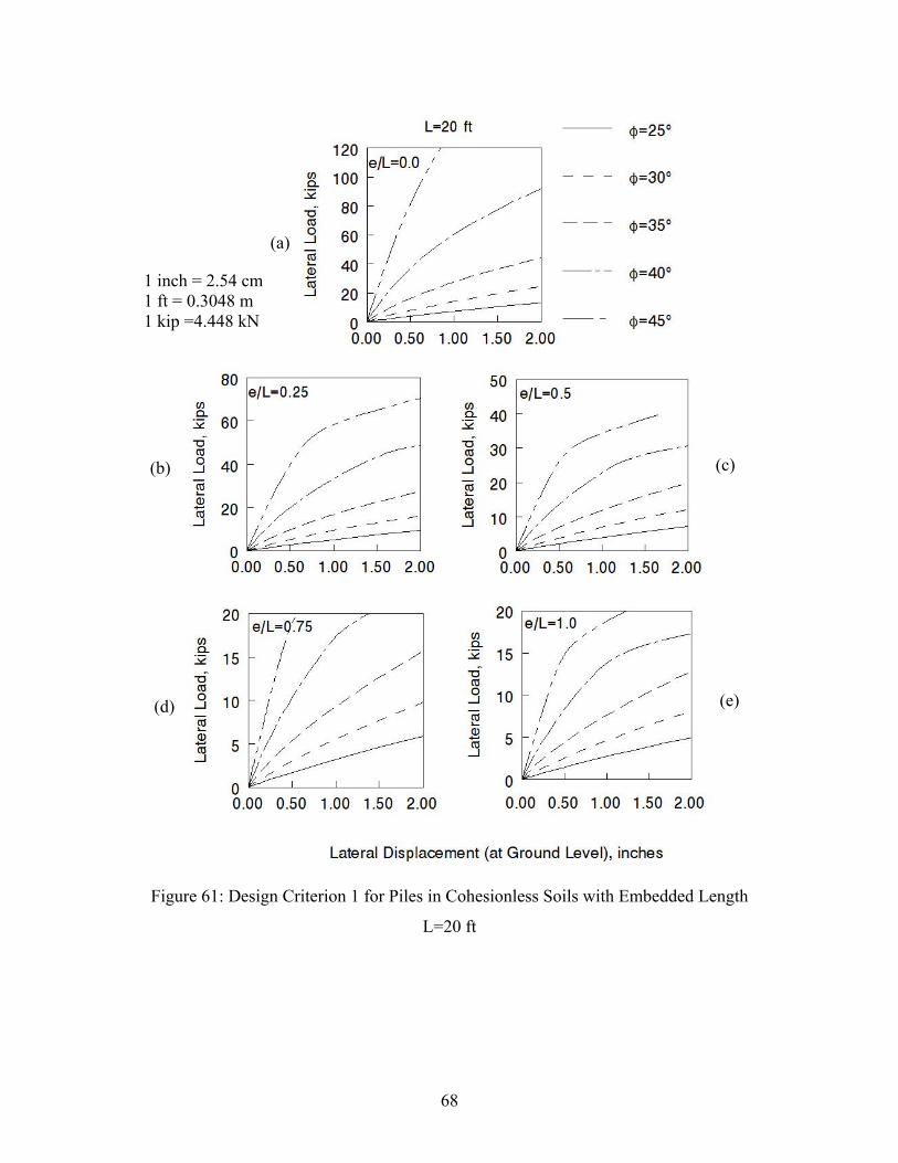
(a)
(c)
(e)
1 inch = 2.54 cm 1 ft = 0.3048 m 1 kip =4.448 kN
(b)
(d)
Figure 61: Design Criterion 1 for Piles in Cohesionless Soils with Embedded Length
L=20 ft
68

(a)
(c)
(e)
1 inch = 2.54 cm 1 ft = 0.3048 m 1 kip =4.448 kN
(b)
(d)
Figure 62: Design Criterion 2 for Piles in Cohesionless Soils with Embedded Length
L=20 ft
69

(a)
(c)
(e)
1 inch = 2.54 cm 1 ft = 0.3048 m 1 kip =4.448 kN
(b)
(d)
Figure 63: Design Criterion 1 for Piles in Cohesionless Soils with Embedded Length
L=30 ft
70

(a)
(c)
(e)
1 inch = 2.54 cm 1 ft = 0.3048 m 1 kip =4.448 kN
(b)
(d)
Figure 64: Design Criterion 2 for Piles in Cohesionless Soils with Embedded Length
L=30 ft
71
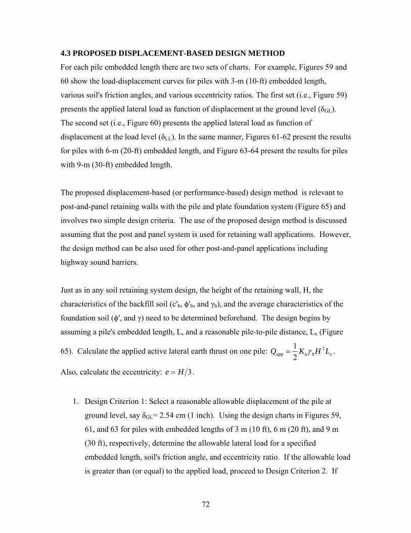
4.3 PROPOSED DISPLACEMENT-BASED DESIGN METHOD
For each pile embedded length there are two sets of charts. For example, Figures 59 and
60 show the load-displacement curves for piles with 3-m (10-ft) embedded length,
various soil's friction angles, and various eccentricity ratios. The first set (i.e., Figure 59)
presents the applied lateral load as function of displacement at the ground level (δGL).
The second set (i.e., Figure 60) presents the applied lateral load as function of
displacement at the load level (δLL). In the same manner, Figures 61-62 present the results
for piles with 6-m (20-ft) embedded length, and Figure 63-64 present the results for piles
with 9-m (30-ft) embedded length.
The proposed displacement-based (or performance-based) design method is relevant to
post-and-panel retaining walls with the pile and plate foundation system (Figure 65) and
involves two simple design criteria. The use of the proposed design method is discussed
assuming that the post and panel system is used for retaining wall applications. However,
the design method can be also used for other post-and-panel applications including
highway sound barriers.
Just as in any soil retaining system design, the height of the retaining wall, H, the
characteristics of the backfill soil (cʹb, ϕʹb, and γb), and the average characteristics of the
foundation soil (ϕʹ, and γ) need to be determined beforehand. The design begins by
assuming a pile's embedded length, L, and a reasonable pile-to-pile distance, Lx (Figure
65). Calculate the applied active lateral earth thrust on one pile: xbaapp LHKQ 2
2
1 .
Also, calculate the eccentricity: 3He .
1. Design Criterion 1: Select a reasonable allowable displacement of the pile at
ground level, say δGL= 2.54 cm (1 inch). Using the design charts in Figures 59,
61, and 63 for piles with embedded lengths of 3 m (10 ft), 6 m (20 ft), and 9 m
(30 ft), respectively, determine the allowable lateral load for a specified
embedded length, soil's friction angle, and eccentricity ratio. If the allowable load
is greater than (or equal) to the applied load, proceed to Design Criterion 2. If
72

2. Design Criterion 2: After determining the allowable lateral load from Design
Criterion 1, determine the at-load-level displacement, δLL, using the design charts
in Figures 60, 62, and 64 for piles with embedded lengths of 3 m (10 ft), 6 m (20
ft), and 9 m (30 ft), respectively. From geometrical considerations (the above-
ground pile length, H, and the eccentricity, e) and using the estimated
displacements δLL and δGL, determine the tilt of the above-ground portion of the
pile. Accept the design if pile tilt is within acceptable limits (1 to 2 %). If tilt is
excessive, then modify L, or Lx, or both L and Lx. Go back to Design Criterion 1.
When the calculated tilt of the pile is large (greater than 2%) the pile with plate
foundation system can be driven at a negative tilt (i.e., towards the backfill). This will
cause the wall to be near vertical after the placement of the backfill soil. This procedure
is not tested yet but it seems fairly feasible.
The use of the proposed design method in cohesionless soils is illustrated in the next two
examples.
Example 1 (Post-and-panel system with a pile with plate foundation in sand):
As shown in Figure 65 the post-and-panel system with a pile with plate foundation type is
used to retain a 4.6-m (15-ft) high backfill. The embedded length of the pile with plate is
6.1 m (20 ft). The friction angle of the sandy foundation soil is 40º as was obtained
from correlations with the average N60 value of 12. The backfill soil unit weight and
strength parameters are shown in the figure. Calculate the required distance between
piles center-to-center. Assume δGL= 2.54 cm (1 inch).
Solution (English units):
Given: L=20 ft, H=15 ft, ϕʹ=40º, δGL= 1 inch
73

Lx=?
ftH
e 53
15
3
25.020
5
L
e
For L=20 ft, ϕʹ=40º, 25.0L
e, and δGL= 1 inch, use Figure 61b (detailed in Figure 66) to
obtain Qall≈33.7 kips.
Set Qapp=Qall, therefore: 2
2 2
2
1
HK
QLLHKQ
ba
appxxbaapp
or, ftLx 6.1015100283.0
3370022
where, 283.034sin1
34sin1
sin1
sin1
b
baK
Use Lx=10 ft.
Performance Issues:
From Figure 62b (detailed in Figure 66) we can estimate the lateral displacement at load
level, δLL≈ 3 inch, corresponding to Qapp=33.7 kips. It is noted from Figure 62b that
Qapp=33.7 kips is below the load that causes the initial yielding of the pile.
From Figure 65 one can estimate the slope of the above-ground portion of the pile and the
lateral deflection at the end of the pile, δtop.
%3.3125
13
Slope
inchestoptop 7
125
13
1215
1
As indicated earlier, when the calculated tilt (slope) of the pile is large, as in this
example, the pile with plate foundation system can be driven at a negative tilt (i.e.,
74

towards the backfill). This will cause the wall to be near vertical after the placement of
the backfill soil.
1 ft = 0.3048 m 1 inch = 2.54 cm 1 lb/ft3 = 0.16 kN/m3
Figure 65: Design Example 1--Pile in Sand
75
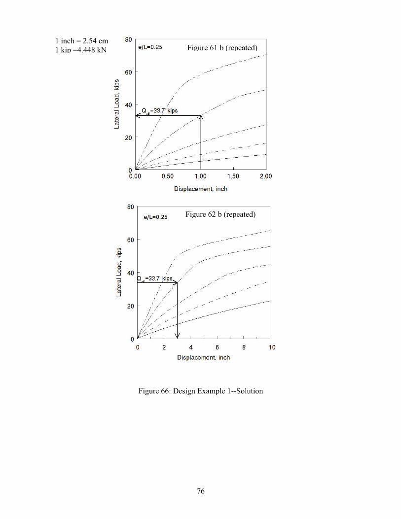
1 inch = 2.54 cm 1 kip =4.448 kN
Figure 62 b (repeated)
Figure 61 b (repeated)
Figure 66: Design Example 1--Solution
76

Example 2 (Post-and-panel system with a pile with plate foundation in sand):
Figure 67 shows a post-and-panel system with a pile with plate foundation type that is
used to retain a 2.3 m (7.5-ft) high backfill. The friction angle of the sandy foundation
soil is 35º. The backfill soil unit weight and strength parameters are shown in the figure.
The distance between piles center-to-center is Lx=6.1 m (20 ft). Calculate the required
embedded length of the pile with plate foundation. The lateral deflection of the pile at
ground level should not exceed 2.54 cm (1 inch).
Solution (English units):
Given: H=7.5 ft, ϕʹ=35º, δGL= 1 inch, and Lx=20 ft
kipsLHKQ xbaapp 7.14205.7110238.05.02
1 22
where, 238.038sin1
38sin1
sin1
sin1
b
baK
ftH
e 5.23
5.7
3
Try L=10 ft
25.010
5.2
L
e
For L=10 ft, ϕʹ=35º, 25.0L
e, and δGL= 1 inch, use Figure 59b to obtain Qall≈14.7 kips.
Therefore, Qapp≈Qall, and the suggested embedded length L=10 ft is acceptable.
Performance Issues:
From Figure 60b we can estimate the lateral displacement at load level, δLL≈ 1.49 inch,
corresponding to Qapp=14.7 kips. It is noted from Figure 60b that Qapp=14.7 kips is below
the load that causes the initial yielding of the pile.
77

From Figure 67 we can estimate the slope of the above-ground portion of the pile and the
lateral deflection at the end of the pile, δtop.
%6.1125.2
149.1
Slope → Okay!
inchestoptop 47.2
125.2
149.1
125.7
1
→ Okay!
1 ft = 0.3048 m 1 inch = 2.54 cm 1 lb/ft3 = 0.16 kN/m3
Figure 67: Design Example 2--Pile in Sand
78

4.4 DESIGN CHARTS FOR THE PILE WITH PLATE SYSTEM: COHESIVE
SOILS
Five cohesive soils with cu=16.7 kPa (350 psf), 30 kPa (625 psf), 65 kPa (1350 psf), 125
kPa (2600 psf), and 210 kPa (4400 psf) are used in this parametric study. As was done in
the previous analyses for cohesionless soils, three embedded lengths of the pile with plate
system are used: 3 m (10 ft), 6 m (20 ft), and 9 m (30 ft). The above-ground length of
each pile is the same as its embedded length. Five eccentricity ratios are used for each
pile: 0, 0.25, 0.5, 0.75, and 1. In total, 75 analyses combinations are considered as
indicated in Table 5.
Table 5: Analysis Matrix for Cohesive Soils
L= 3 m (10 ft) e=0 e=0.25 e=0.5 e=0.75 e=1.0 cu=350 psf L10ft_e0.0_cu1 L10ft_e0.25_ cu1 L10ft_e0.5_ cu1 L10ft_e0.75_ cu1 L10ft_e1.0_ cu1 cu =625 psf L10ft_e0.0_cu2 L10ft_e0.25_ cu2 L10ft_e0.5_ cu2 L10ft_e0.75_ cu2 L10ft_e1.0_ cu2 cu =1350 psf L10ft_e0.0_ cu3 L10ft_e0.25_ cu3 L10ft_e0.5_ cu3 L10ft_e0.75_ cu3 L10ft_e1.0_ cu3 cu =2600 psf L10ft_e0.0_cu4 L10ft_e0.25_ cu4 L10ft_e0.5_ cu4 L10ft_e0.75_ cu4 L10ft_e1.0_ cu4 cu =4400 psf L10ft_e0.0_cu5 L10ft_e0.25_ cu5 L10ft_e0.5_ cu5 L10ft_e0.75_ cu5 L10ft_e1.0_ cu5 L=6 m (20 ft) e=0 e=0.25 e=0.5 e=0.75 e=1.0 cu=350 psf L20ft_e0.0_ cu1 L20ft_e0.25_ cu1 L20ft_e0.5_ cu1 L20ft_e0.75_ cu1 L20ft_e1.0_ cu1 cu =625 psf L20ft_e0.0_ cu2 L20ft_e0.25_ cu2 L20ft_e0.5_ cu2 L20ft_e0.75_ cu2 L20ft_e1.0_ cu2 cu =1350 psf L20ft_e0.0_ cu3 L20ft_e0.25_ cu3 L20ft_e0.5_ cu3 L20ft_e0.75_ cu3 L20ft_e1.0_ cu3 cu =2600 psf L20ft_e0.0_ cu4 L20ft_e0.25_ cu4 L20ft_e0.5_ cu4 L20ft_e0.75_ cu4 L20ft_e1.0_ cu4 cu =4400 psf L20ft_e0.0_ cu5 L20ft_e0.25_ cu5 L20ft_e0.5_ cu5 L20ft_e0.75_ cu5 L20ft_e1.0_ cu5 L=9 m (30 ft) e=0 e=0.25 e=0.5 e=0.75 e=1.0 cu=350 psf L30ft_e0.0_ cu1 L30ft_e0.25_ cu1 L30ft_e0.5_ cu1 L30ft_e0.75_ cu1 L30ft_e1.0_ cu1 cu =625 psf L30ft_e0.0_ cu2 L30ft_e0.25_ cu2 L30ft_e0.5_ cu2 L30ft_e0.75_ cu2 L30ft_e1.0_ cu2 cu =1350 psf L30ft_e0.0_ cu3 L30ft_e0.25_ cu3 L30ft_e0.5_ cu3 L30ft_e0.75_ cu3 L30ft_e1.0_ cu3 cu =2600 psf L30ft_e0.0_ cu4 L30ft_e0.25_ cu4 L30ft_e0.5_ cu4 L30ft_e0.75_ cu4 L30ft_e1.0_ cu4 cu =4400 psf L30ft_e0.0_ cu5 L30ft_e0.25_ cu5 L30ft_e0.5_ cu5 L30ft_e0.75_ cu5 L30ft_e1.0_ cu5
79

For all parametric analyses the soil is assumed to be homogeneous. A step-be-step
procedure, presented below, is used here to estimate soil parameters based on N60-values
as shown in Table 6.
Table 6: Cap Model Parameters for Parametric Analyses (Cohesive Soils)
Soil Description cu (psf) N60 d (psf) E (psf) Very soft clay 350 1 600 2.265E+04 Soft clay 625 3 1087 5.173E+04 Medium clay 1350 8 2346 1.505E+05 Stiff clay 2600 20 4521 3.743E+05 Very stiff clay 4400 41 7608 7.712E+05
A step-by-step procedure to obtain cohesive soil parameters:
1. From SPT soundings, divide the soil into layers based on N60. Calculate the weighted
average of the N60-value for the soil strata.
2. Calculate the undrained cohesion of the soil strata: 72.060 )( (Hara et al,
1971).
29)( NkPacu
3. As a safety precaution, use a modified undrained cohesion (cu)mod, such that:
2
)(29
2
)()()(
72.060
mod
NkPackPac u
u . This safety factor is introduced herein
because of the lack of experience using the proposed pile with plate system in
cohesive soils.
4. Calculate the cohesion constant for the modified Drucker-Prager/Cap soil model:
mod)(3 ucd .
5. Calculate the friction angle for the modified Drucker-Prager/Cap soil model:
0]sin3
sin6[tan 1
u
u
, where ϕu is the undrained friction angle of the soil (=0).
6. Reasonable elastic modulus of the soil can be assumed. The values given in Table 6
are on the lower bound of elastic moduli for clays based on the written literature.
80

As was done in the parametric analyses for cohesionless soils, a 2.54 cm (1-inch) thick
plate welded to an H-beam (HP12×53) with the proper embedment length is used in all
analyses. A36 mild steel properties (Figure 54) are used for the beam and the plate in all
analyses. For each of the 75 finite element analyses indicated in Table 5, the finite
element mesh (similar to the one shown in Figure 55) is adjusted to accommodate
different soils, different pile embedded length, and different eccentricity ratios. The
analytical results are presented as "Design Charts" shown in Figures 68 to 73.
The proposed two-criteria displacement-based design method, described above, can also
be used for the design of post-and-panel retaining walls with the pile and plate foundation
system embedded in cohesive soils. As described earlier, the method involves two
simple design criteria. Figures 68, 70, and 72 are associated with design criterion 1,
whereas Figures 69, 71, and 73 are associated with design criterion 2. The use of the
proposed design method in a cohesive soil is illustrated in the next example.
81

(a)
(c)
(e)
1 inch = 2.54 cm 1 ft = 0.3048 m 1 kip =4.448 kN
(b)
(d)
Figure 68: Design Criterion 1 for Piles in Cohesive Soils with Embedded Length L=10 ft
82

(a)
(c)
(e)
1 inch = 2.54 cm 1 ft = 0.3048 m 1 kip =4.448 kN
(b)
(d)
Figure 69: Design Criterion 2 for Piles in Cohesive Soils with Embedded Length L=10 ft
83

(a)
(c)
(e)
1 inch = 2.54 cm 1 ft = 0.3048 m 1 kip =4.448 kN
(b)
(d)
Figure 70: Design Criterion 1 for Piles in Cohesive Soils with Embedded Length L=20 ft
84
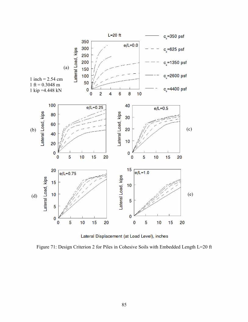
(a)
(c)
(e)
1 inch = 2.54 cm 1 ft = 0.3048 m 1 kip =4.448 kN
(b)
(d)
Figure 71: Design Criterion 2 for Piles in Cohesive Soils with Embedded Length L=20 ft
85

(a)
(c)
(e)
1 inch = 2.54 cm 1 ft = 0.3048 m 1 kip =4.448 kN
(b)
(d)
Figure 72: Design Criterion 1 for Piles in Cohesive Soils with Embedded Length L=30 ft
86

(a)
Figure 73: Design Criterion 2 for Piles in Cohesive Soils with Embedded Length L=30 ft
(b) (c)
(e)
1 inch = 2.54 cm 1 ft = 0.3048 m 1 kip =4.448 kN
(d)
87

Example 3 (Post-and-panel system with a pile with plate foundation in clay):
As shown in Figure 74 the post-and-panel system with a pile with plate foundation type is
used to retain a 4.6-m (15-ft) high backfill. The embedded length of the pile with plate is
6.1 m (20 ft). The average undrained cohesion of the clayey foundation soil is 1350 psf
as was obtained from correlations with the average N60 value of the soil strata in the
vicinity of the embedded length of the foundation system. The backfill soil unit weight
and strength parameters are shown in the figure. Calculate the required distance between
piles center-to-center. Assume δGL= 2.54 cm (1 inch).
Solution (English units):
Given: L=20 ft, H=15 ft, cu=1350 psf, δGL= 1 inch
Lx=?
ftH
e 53
15
3
25.020
5
L
e
For L=20 ft, cu=1350 psf, 25.0L
e, and δGL= 1 inch, use Figure 70b to obtain Qall≈36
kips.
Set Qapp=Qall, therefore: 2
2 2
2
1
HK
QLLHKQ
ba
appxxbaapp
or, ftLx 3.1115100283.0
3600022
where, 283.034sin1
34sin1
sin1
sin1
b
baK
Use Lx=10 ft.
88
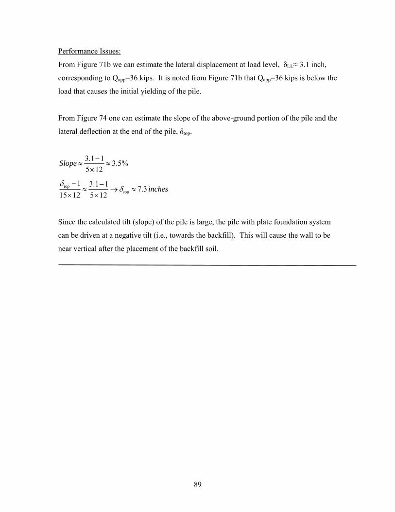
Performance Issues:
From Figure 71b we can estimate the lateral displacement at load level, δLL≈ 3.1 inch,
corresponding to Qapp=36 kips. It is noted from Figure 71b that Qapp=36 kips is below the
load that causes the initial yielding of the pile.
From Figure 74 one can estimate the slope of the above-ground portion of the pile and the
lateral deflection at the end of the pile, δtop.
%5.3125
11.3
Slope
inchestoptop 3.7
125
11.3
1215
1
Since the calculated tilt (slope) of the pile is large, the pile with plate foundation system
can be driven at a negative tilt (i.e., towards the backfill). This will cause the wall to be
near vertical after the placement of the backfill soil.
89

1 ft = 0.3048 m 1 inch = 2.54 cm 1 lb/ft3 = 0.16 kN/m3
Figure 74: Design Example 3--Pile in Clay
90

91
REFERENCES
Broms, B.B. (1964). “Design of Laterally Loaded Piles,” Journal of the Soil Mechanics and Foundation Division, American Society of Civil Engineers, Vol. 91, No. SM3, pp. 79-99. Davisson, M.T., and Gill, H.L. (1963). “Laterally Loaded Piles in a Layered Soil System,” Journal of the Soil Mechanics and Foundation Division, American Society of Civil Engineers, Vol. 89, No. SM3, pp. 63-94. Hara, A., Ohta, T., and Niwa, M. (1971). "Shear Modulus and Shear Strength of Cohesive Soils," Soils and Foundations, Vol. 14, No. 3, pp. 1-12. Kulhawy, F.H., and Myane, P.W. (1990). Manual on Estimating Soil Properties for Foundation Design, Electric Power Research Institute, Palo Alto, California. Matlock, H., and Reese, L.C. (1960). “Generalized Solution for Laterally Loaded Piles,” Journal of the Soil Mechanics and Foundation Division, American Society of Civil Engineers, Vol. 86, No. SM5, pp. 63-91. Meyerhof, G. G. (1995). “Behavior of Pile Foundations under Special Loading Conditions: 1994 R.M. Hardy Keynote Address,” Canadian Geotechnical Journal, Vol. 32, No. 2, pp. 204-222. Robertson, P.K., and Campanella, R.G. (1983). "Interpretation of Cone Penetration Tests. Part I: Sand, " Canadian Geotechnical Journal, Vol. 20, No. 4, pp. 718-733. Schmertmann, J.H. (1970). Static cone to compute static settlement over sand. ASCE Journal of Soil Mechanics & Foundations Division 96 (3), 1011-1043.

Appendix A Site Investigation

Borings at E. Bay Street and Lincoln Memorial Drive

1
SW-SM
SM
19
2
Gra
phic
6
7
11
11
32
9
ENGINEERS ARCHITECTS PLANNERS
24
N -
Val
ue
Rec
over
y(in
)
No recovery @ 10-12 feetsample interval
5
10
15
20
No recovery in Shelby Tube
Page 1 of 5B-1
4 in.
BORING NUMBER
SURFACE ELEVATION
PROJECT NUMBER
Num
ber
and
Type
Hard, brown CLAY/SILT FILL, little fine gravel, moist
SP
T - 3
SP
T - 2
SP
T - 1
Medium dense to very dense well-graded SAND withsilt, trace organics (marine shells), moist
SP
T - 5
Very loose to loose, dark brown to black silty SAND,little to some fine to coarse gravel, trace organics,moist to wet (Possible Fill)
SP
T - 6
Dense, gray to brown GRANULAR FILL, fine tocoarse sand and gravel, moist
24
24
0
24
0
24
12
24
24
- with trace fine gravel
|
41991
|
|
|
|
|
SP
T - 4
|
|
|
SP
T - 1
0S
PT
- 9S
H -
8S
PT
- 7
|
US
CS
BORING DRILLED BY
Comments
Liqu
id L
imit
FIRM: WisDOTCREW CHIEF: Skolos LAB LOG / QC
4/6/2009
NOTE: Bolded Unconfined Compressive Strength values denote a Qp test.NOTE: Stratification lines between soil types represent the approximate boundary; gradual transition between in-situ soil layers should be expected.
Pla
stic
ity In
dex
11414 West Park Place, Ste. 300, Milwaukee, WI 53224Phone (414) 359-2300 Fax (414) 359-2310
HN
TB G
EO
TEC
H S
BL
W
HR
P 2
009
BO
RIN
GS
.GP
J
HN
TB-W
IDN
R.G
DT
5/
20/0
9
Unc
onfin
ed C
ompr
essi
ve S
treng
th(Q
u or
Qp)
(tsf
)
Wisconsin Highway Research Project
CAVE DEPTH AT COMPLETION: ft.
SOIL BORING LOG
Moi
stur
e C
onte
nt(%
)
NORTHING
WATER LEVEL AFTER HOURS: ft., hrs.
Dep
th (f
t)
Ele
vatio
n
Blo
w C
ount
s
EASTING
Wel
l Dia
gram
4/7/2009
WATER OBSERVATION DATAWETDRYWATER ENCOUNTERED DURING DRILLING: 8 ft.
WATER LEVEL AT COMPLETION: ft.
DRILL RIG
wash boringDRILLING METHOD
Soil Descriptionand Geological Origin for
Each Major Unit
WETDRY
SDM/DAJ
DATE DRILLING STARTED
CAVE DEPTH AFTER HOURS: ft., hrs.
Skolos
PROJECT NAME
BOREHOLE DIAMETERFIELD LOG
Feet
DATE DRILLING ENDED
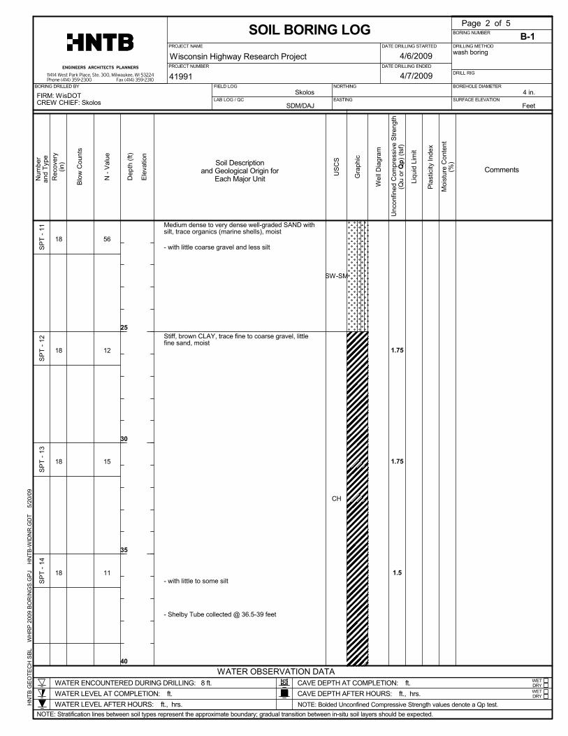
Page 2 of 5
N -
Val
ue
Rec
over
y(in
)ENGINEERS ARCHITECTS PLANNERS
B-1
4 in.
BORING NUMBER
SURFACE ELEVATION
PROJECT NUMBER
25
30
35
40
18
wash boringDRILLING METHOD
41991
Soil Descriptionand Geological Origin for
Each Major Unit Gra
phic
Num
ber
and
Type
1.5
1.75
1.75
SP
T - 1
4S
PT
- 13
|
SP
T - 1
1
|
- Shelby Tube collected @ 36.5-39 feet
- with little to some silt
Stiff, brown CLAY, trace fine to coarse gravel, littlefine sand, moist
- with little coarse gravel and less silt
Medium dense to very dense well-graded SAND withsilt, trace organics (marine shells), moist
18
18
18
SP
T - 1
2
CH
SW-SM
11
15
12
56
|
|
|
Comments
WATER LEVEL AT COMPLETION: ft.
Liqu
id L
imit
FIRM: WisDOTCREW CHIEF: Skolos LAB LOG / QC
4/6/2009
11414 West Park Place, Ste. 300, Milwaukee, WI 53224Phone (414) 359-2300 Fax (414) 359-2310
HN
TB G
EO
TEC
H S
BL
W
HR
P 2
009
BO
RIN
GS
.GP
J
HN
TB-W
IDN
R.G
DT
5/
20/0
9
Unc
onfin
ed C
ompr
essi
ve S
treng
th(Q
u or
Qp)
(tsf
)
Wisconsin Highway Research Project
CAVE DEPTH AT COMPLETION: ft.
Blo
w C
ount
s
SOIL BORING LOG
Dep
th (f
t)
Ele
vatio
n
Moi
stur
e C
onte
nt(%
)
Pla
stic
ity In
dex
WATER LEVEL AFTER HOURS: ft., hrs. NOTE: Bolded Unconfined Compressive Strength values denote a Qp test.
US
CS
WETDRY
BOREHOLE DIAMETERFIELD LOG
DATE DRILLING ENDED
PROJECT NAME
EASTING
Wel
l Dia
gram
4/7/2009
WATER OBSERVATION DATAWETDRYWATER ENCOUNTERED DURING DRILLING: 8 ft.
DRILL RIG
NORTHINGBORING DRILLED BY
Feet
NOTE: Stratification lines between soil types represent the approximate boundary; gradual transition between in-situ soil layers should be expected.
DATE DRILLING STARTED
CAVE DEPTH AFTER HOURS: ft., hrs.
Skolos
SDM/DAJ

45
50
55
60
ENGINEERS ARCHITECTS PLANNERS
N -
Val
ue
Rec
over
y(in
)
Gra
phic
Page 3 of 5B-1
4 in.
BORING NUMBER
SURFACE ELEVATION
18
wash boringDRILLING METHOD
41991
Num
ber
and
Type Soil Description
and Geological Origin forEach Major Unit
SP
T - 1
6
|
2.5
1.5
1.25
1
SP
T - 1
7
|
SP
T - 1
5
Very stiff to hard, brownish gray silty CLAY, little finesand, moist
Stiff, brown CLAY, trace fine to coarse gravel, littlefine sand, moist
18
18
18
SP
T - 1
8
WATER LEVEL AT COMPLETION: ft.
CL
CH
19
14
|
10
|
PROJECT NUMBER
1.25
Comments
WATER ENCOUNTERED DURING DRILLING: 8 ft.
Liqu
id L
imit
FIRM: WisDOTCREW CHIEF: Skolos LAB LOG / QC
4/6/2009
11414 West Park Place, Ste. 300, Milwaukee, WI 53224Phone (414) 359-2300 Fax (414) 359-2310
HN
TB G
EO
TEC
H S
BL
W
HR
P 2
009
BO
RIN
GS
.GP
J
HN
TB-W
IDN
R.G
DT
5/
20/0
9
Unc
onfin
ed C
ompr
essi
ve S
treng
th(Q
u or
Qp)
(tsf
)
Wisconsin Highway Research Project
CAVE DEPTH AT COMPLETION: ft.
Blo
w C
ount
s
SOIL BORING LOG
Dep
th (f
t)
Ele
vatio
n
Moi
stur
e C
onte
nt(%
)
Pla
stic
ity In
dex
WATER LEVEL AFTER HOURS: ft., hrs. NOTE: Bolded Unconfined Compressive Strength values denote a Qp test.
DATE DRILLING ENDED
US
CS
WETDRY
BOREHOLE DIAMETER
NOTE: Stratification lines between soil types represent the approximate boundary; gradual transition between in-situ soil layers should be expected.
PROJECT NAME
EASTING
Wel
l Dia
gram
4/7/2009
WATER OBSERVATION DATAWETDRY
FIELD LOG
DRILL RIG
NORTHINGBORING DRILLED BY
SDM/DAJ
DATE DRILLING STARTED
CAVE DEPTH AFTER HOURS: ft., hrs.
Skolos
Feet

65
70
75
80
ENGINEERS ARCHITECTS PLANNERS
N -
Val
ue
Rec
over
y(in
)
Gra
phic
Page 4 of 5B-1
4 in.
BORING NUMBER
SURFACE ELEVATION
18
wash boringDRILLING METHOD
41991
Num
ber
and
Type Soil Description
and Geological Origin forEach Major Unit
SP
T - 2
0
|
0.5
4.5
3.5
0.5
SP
T - 2
1
|
SP
T - 1
9
Medium dense, gray silty SAND with clay, wet
- with wet silt seam
Very stiff to hard, brownish gray silty CLAY, little finesand, moist
18
18
18
SP
T - 2
2
WATER LEVEL AT COMPLETION: ft.
SM
CL
27
40
|
24
|
PROJECT NUMBER
28
Comments
WATER ENCOUNTERED DURING DRILLING: 8 ft.
Liqu
id L
imit
FIRM: WisDOTCREW CHIEF: Skolos LAB LOG / QC
4/6/2009
11414 West Park Place, Ste. 300, Milwaukee, WI 53224Phone (414) 359-2300 Fax (414) 359-2310
HN
TB G
EO
TEC
H S
BL
W
HR
P 2
009
BO
RIN
GS
.GP
J
HN
TB-W
IDN
R.G
DT
5/
20/0
9
Unc
onfin
ed C
ompr
essi
ve S
treng
th(Q
u or
Qp)
(tsf
)
Wisconsin Highway Research Project
CAVE DEPTH AT COMPLETION: ft.
Blo
w C
ount
s
SOIL BORING LOG
Dep
th (f
t)
Ele
vatio
n
Moi
stur
e C
onte
nt(%
)
Pla
stic
ity In
dex
WATER LEVEL AFTER HOURS: ft., hrs. NOTE: Bolded Unconfined Compressive Strength values denote a Qp test.
DATE DRILLING ENDED
US
CS
WETDRY
BOREHOLE DIAMETER
NOTE: Stratification lines between soil types represent the approximate boundary; gradual transition between in-situ soil layers should be expected.
PROJECT NAME
EASTING
Wel
l Dia
gram
4/7/2009
WATER OBSERVATION DATAWETDRY
FIELD LOG
DRILL RIG
NORTHINGBORING DRILLED BY
SDM/DAJ
DATE DRILLING STARTED
CAVE DEPTH AFTER HOURS: ft., hrs.
Skolos
Feet

DRILLING METHODwash boring
Gra
phic
41991
Soil Descriptionand Geological Origin for
Each Major Unit
WATER ENCOUNTERED DURING DRILLING: 8 ft.
ENGINEERS ARCHITECTS PLANNERS
18
Wel
l Dia
gram
4/7/2009
WETDRY
WATER LEVEL AT COMPLETION: ft.
WATER OBSERVATION DATA
GW-GM
SM
27
SP
T - 2
3
End of Boring @ 82 feet
Medium dense, gray well-graded GRAVEL withsand, little to some silt, wet
Medium dense, gray silty SAND with clay, wet|
4 in.
N -
Val
ue
Rec
over
y(in
)
85
90
95
100
B-1BORING NUMBER
SURFACE ELEVATION
PROJECT NUMBER
Num
ber
and
Type
Page 5 of 5
LAB LOG / QC
Dep
th (f
t)
Ele
vatio
n
Blo
w C
ount
s
Comments
Liqu
id L
imit
EASTING
SOIL BORING LOG
11414 West Park Place, Ste. 300, Milwaukee, WI 53224Phone (414) 359-2300 Fax (414) 359-2310
HN
TB G
EO
TEC
H S
BL
W
HR
P 2
009
BO
RIN
GS
.GP
J
HN
TB-W
IDN
R.G
DT
5/
20/0
9
Unc
onfin
ed C
ompr
essi
ve S
treng
th(Q
u or
Qp)
(tsf
)
Wisconsin Highway Research Project
FIRM: WisDOTCREW CHIEF: Skolos
Moi
stur
e C
onte
nt(%
)
Pla
stic
ity In
dex
WATER LEVEL AFTER HOURS: ft., hrs.
CAVE DEPTH AT COMPLETION: ft.
DATE DRILLING ENDED
DATE DRILLING STARTED
CAVE DEPTH AFTER HOURS: ft., hrs.
Skolos
PROJECT NAME
WETDRY
BOREHOLE DIAMETERFIELD LOG
DRILL RIG
NOTE: Stratification lines between soil types represent the approximate boundary; gradual transition between in-situ soil layers should be expected.
4/6/2009
US
CS
NOTE: Bolded Unconfined Compressive Strength values denote a Qp test.
NORTHINGBORING DRILLED BY
FeetSDM/DAJ

16
SW-SM
SM
100
4
8
9
7
Num
ber
and
Type
65
19
37
8
5
10
15
20
ENGINEERS ARCHITECTS PLANNERS
24
N -
Val
ue
Rec
over
y(in
)
Petroleum odor noted @14-20 feet
Page 1 of 5B-2
4 in.
BORING NUMBER
SURFACE ELEVATION
PROJECT NUMBER
Dense to loose, light brown to black GRANULARFILL, fine to coarse sand and gravel, dry to moist
SP
T - 2
SP
T - 1
Very dense, light to dark gray SAND with gravel, fineto coarse sand and gravel, some silt, cementedconcrete fragments, wet (Possible Fill)
Loose, black to gray silty SAND, moist to wet(Possible Fill)
- with petroleum odor
- with slag and foundry sand
- with black foundry sand and glass fragments
SP
T - 5
2
24
6
6
12
24
24
24
24
- with nails and foundry sand
|
|
|
|
|
|
|
SP
T - 3
|
SP
T - 4
|
SP
T - 1
0S
PT
- 9S
PT
- 8S
PT
- 7S
PT
- 6
Gra
phic
|
US
CS
Comments
Liqu
id L
imit
FIRM: WisDOTCREW CHIEF: Skolos LAB LOG / QC
4/7/2009
NOTE: Bolded Unconfined Compressive Strength values denote a Qp test.NOTE: Stratification lines between soil types represent the approximate boundary; gradual transition between in-situ soil layers should be expected.
41991
Pla
stic
ity In
dex
11414 West Park Place, Ste. 300, Milwaukee, WI 53224Phone (414) 359-2300 Fax (414) 359-2310
HN
TB G
EO
TEC
H S
BL
W
HR
P 2
009
BO
RIN
GS
.GP
J
HN
TB-W
IDN
R.G
DT
5/
20/0
9
Unc
onfin
ed C
ompr
essi
ve S
treng
th(Q
u or
Qp)
(tsf
)
Wisconsin Highway Research Project
CAVE DEPTH AT COMPLETION: ft.
SOIL BORING LOG
Moi
stur
e C
onte
nt(%
)
WATER LEVEL AFTER HOURS: ft., hrs.
Dep
th (f
t)
Ele
vatio
n
Blo
w C
ount
sNORTHING
EASTING
Wel
l Dia
gram
4/8/2009
WATER OBSERVATION DATAWETDRYWATER ENCOUNTERED DURING DRILLING: ft.
WATER LEVEL AT COMPLETION: ft.
DRILL RIG
wash boringDRILLING METHOD
Soil Descriptionand Geological Origin for
Each Major Unit
FeetSDM/DAJ
DATE DRILLING STARTED
CAVE DEPTH AFTER HOURS: ft., hrs.
Skolos
DATE DRILLING ENDED
WETDRY
BOREHOLE DIAMETERFIELD LOGBORING DRILLED BY
PROJECT NAME

Page 2 of 5
N -
Val
ue
Rec
over
y(in
)
Num
ber
and
Type
B-2
4 in.
BORING NUMBER
SURFACE ELEVATION
ENGINEERS ARCHITECTS PLANNERS
25
30
35
40
24
wash boringDRILLING METHOD
41991
Soil Descriptionand Geological Origin for
Each Major Unit Gra
phic
|
|
SP
T - 1
5S
PT
- 14
SP
T - 1
3
PROJECT NUMBER
SP
T - 1
1
|
- with trace fine gravel
Medium, grayish brown CLAY, some fine sand, littlefine gravel, moist
Very dense, light to dark gray SAND with gravel, fineto coarse sand and gravel, some silt, cementedconcrete fragments, wet (Possible Fill)
18
18
24
24
SP
T - 1
2
CH
SW-SM
15
15
14
101
|
|
|
65
Comments
WATER LEVEL AT COMPLETION: ft.
Liqu
id L
imit
FIRM: WisDOTCREW CHIEF: Skolos LAB LOG / QC
4/7/2009
11414 West Park Place, Ste. 300, Milwaukee, WI 53224Phone (414) 359-2300 Fax (414) 359-2310
HN
TB G
EO
TEC
H S
BL
W
HR
P 2
009
BO
RIN
GS
.GP
J
HN
TB-W
IDN
R.G
DT
5/
20/0
9
Unc
onfin
ed C
ompr
essi
ve S
treng
th(Q
u or
Qp)
(tsf
)
Wisconsin Highway Research Project
CAVE DEPTH AT COMPLETION: ft.
Blo
w C
ount
s
SOIL BORING LOG
Dep
th (f
t)
Ele
vatio
n
Moi
stur
e C
onte
nt(%
)
Pla
stic
ity In
dex
WATER LEVEL AFTER HOURS: ft., hrs. NOTE: Bolded Unconfined Compressive Strength values denote a Qp test.
DATE DRILLING ENDED
US
CS
WETDRY
BOREHOLE DIAMETERFIELD LOG
NOTE: Stratification lines between soil types represent the approximate boundary; gradual transition between in-situ soil layers should be expected.
PROJECT NAME
EASTING
Wel
l Dia
gram
4/8/2009
WATER OBSERVATION DATAWETDRYWATER ENCOUNTERED DURING DRILLING: ft.
DRILL RIG
NORTHINGBORING DRILLED BY
Feet
DATE DRILLING STARTED
CAVE DEPTH AFTER HOURS: ft., hrs.
Skolos
SDM/DAJ

B-2
N -
Val
ue
Rec
over
y(in
)
45
50
55
60
Page 3 of 5
41991
4 in.
BORING NUMBER
SURFACE ELEVATION
PROJECT NUMBER
Num
ber
and
Type
ENGINEERS ARCHITECTS PLANNERS
18
wash boringDRILLING METHOD
Soil Descriptionand Geological Origin for
Each Major Unit Gra
phic
SP
T - 1
6
2.5
0.25
0.5
SP
T - 1
9
|
SP
T - 1
7
|
Very stiff to hard, gray silty CLAY, litte to some finesand, moist to wet
Soft, gray silty CLAY, little to some fine sand, moist
Medium, grayish brown CLAY, some fine sand, littlefine gravel, moist
18
18
18
SP
T - 1
8
CL
CL
CH
22
18
12
|
|
12
NOTE: Stratification lines between soil types represent the approximate boundary; gradual transition between in-situ soil layers should be expected.
Comments
Blo
w C
ount
s
Liqu
id L
imit
Dep
th (f
t)
Ele
vatio
n
FIRM: WisDOTCREW CHIEF: Skolos LAB LOG / QC
4/7/2009
11414 West Park Place, Ste. 300, Milwaukee, WI 53224Phone (414) 359-2300 Fax (414) 359-2310
HN
TB G
EO
TEC
H S
BL
W
HR
P 2
009
BO
RIN
GS
.GP
J
HN
TB-W
IDN
R.G
DT
5/
20/0
9
Unc
onfin
ed C
ompr
essi
ve S
treng
th(Q
u or
Qp)
(tsf
)
Wisconsin Highway Research Project
CAVE DEPTH AT COMPLETION: ft.
SOIL BORING LOG
NOTE: Bolded Unconfined Compressive Strength values denote a Qp test.
Moi
stur
e C
onte
nt(%
)
Pla
stic
ity In
dex
WATER LEVEL AFTER HOURS: ft., hrs.
4/8/2009
WATER LEVEL AT COMPLETION: ft.
US
CS
WATER ENCOUNTERED DURING DRILLING: ft.WETDRY
WETDRY
WATER OBSERVATION DATA
DATE DRILLING ENDED
BOREHOLE DIAMETER
PROJECT NAME
FIELD LOG
EASTING
Wel
l Dia
gram
DRILL RIG
NORTHINGBORING DRILLED BY
SDM/DAJ
DATE DRILLING STARTED
CAVE DEPTH AFTER HOURS: ft., hrs.
Skolos
Feet
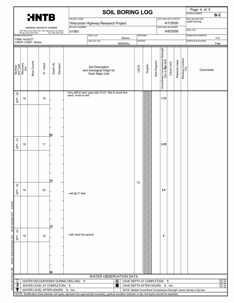
SURFACE ELEVATION
41991
Rec
over
y(in
)
65
70
75
80
Page 4 of 5B-2
4 in.
WETDRY
N -
Val
ue
18
WATER LEVEL AT COMPLETION: ft.
Gra
phic
DRILLING METHOD
Soil Descriptionand Geological Origin for
Each Major Unit
wash boringS
PT
- 21
BORING NUMBER
|
4
2.5
2.25
1.75
|
SP
T - 2
2
|
SP
T - 2
0
- with trace fine gravel
- wet @ 71 feet
Very stiff to hard, gray silty CLAY, litte to some finesand, moist to wet
18
18
18
SP
T - 2
3
PROJECT NUMBER
Num
ber
and
Type
CL
32
20
|
19
WATER OBSERVATION DATA
17
Liqu
id L
imit
4/7/2009
Dep
th (f
t)
Ele
vatio
n
FIRM: WisDOTCREW CHIEF: Skolos LAB LOG / QC
WATER ENCOUNTERED DURING DRILLING: ft.
Comments
11414 West Park Place, Ste. 300, Milwaukee, WI 53224Phone (414) 359-2300 Fax (414) 359-2310
HN
TB G
EO
TEC
H S
BL
W
HR
P 2
009
BO
RIN
GS
.GP
J
HN
TB-W
IDN
R.G
DT
5/
20/0
9
Unc
onfin
ed C
ompr
essi
ve S
treng
th(Q
u or
Qp)
(tsf
)
Wisconsin Highway Research Project
CAVE DEPTH AT COMPLETION: ft.
Blo
w C
ount
s
SOIL BORING LOG
NOTE: Bolded Unconfined Compressive Strength values denote a Qp test.
Moi
stur
e C
onte
nt(%
)
Pla
stic
ity In
dex
WATER LEVEL AFTER HOURS: ft., hrs.
US
CS
PROJECT NAME
DATE DRILLING ENDED
WETDRY
BOREHOLE DIAMETERSkolos
FIELD LOG
CAVE DEPTH AFTER HOURS: ft., hrs.
EASTING
Wel
l Dia
gram
4/8/2009
Feet
NOTE: Stratification lines between soil types represent the approximate boundary; gradual transition between in-situ soil layers should be expected.
DRILL RIG
NORTHINGBORING DRILLED BY
ENGINEERS ARCHITECTS PLANNERS
SDM/DAJ
DATE DRILLING STARTED

wash boringDRILLING METHOD
41991
Soil Descriptionand Geological Origin for
Each Major Unit Gra
phic
ENGINEERS ARCHITECTS PLANNERS
WATER OBSERVATION DATA
18
EASTING
Wel
l Dia
gram
4/8/2009
WETDRYWATER ENCOUNTERED DURING DRILLING: ft.
WATER LEVEL AT COMPLETION: ft.
|
Num
ber
and
Type
CL43 4.5
SP
T - 2
4
End of Boring @ 81.5 feet
Very stiff to hard, gray silty CLAY, litte to some finesand, moist to wet
N -
Val
ue
Rec
over
y(in
)PROJECT NUMBER
85
90
95
100
Page 5 of 5B-2
4 in.
BORING NUMBER
SURFACE ELEVATION
FIELD LOG
Dep
th (f
t)
Ele
vatio
n
Blo
w C
ount
s
Comments
Liqu
id L
imit
SOIL BORING LOG
11414 West Park Place, Ste. 300, Milwaukee, WI 53224Phone (414) 359-2300 Fax (414) 359-2310
HN
TB G
EO
TEC
H S
BL
W
HR
P 2
009
BO
RIN
GS
.GP
J
HN
TB-W
IDN
R.G
DT
5/
20/0
9
Unc
onfin
ed C
ompr
essi
ve S
treng
th(Q
u or
Qp)
(tsf
)
Wisconsin Highway Research Project
Moi
stur
e C
onte
nt(%
)
Pla
stic
ity In
dex
WATER LEVEL AFTER HOURS: ft., hrs.
FIRM: WisDOTCREW CHIEF: Skolos
CAVE DEPTH AT COMPLETION: ft.
DATE DRILLING STARTED
Skolos
SDM/DAJ
PROJECT NAME
DATE DRILLING ENDED
WETDRY
BOREHOLE DIAMETER
CAVE DEPTH AFTER HOURS: ft., hrs.
US
CS
4/7/2009
NOTE: Bolded Unconfined Compressive Strength values denote a Qp test.NOTE: Stratification lines between soil types represent the approximate boundary; gradual transition between in-situ soil layers should be expected.
LAB LOG / QC
DRILL RIG
NORTHINGBORING DRILLED BY
Feet

LABORATORY SOIL TEST REQUEST SHEET
Job No. 41991 Project Location
Wisconsin Highway Research Project (WHRP)
DATE 5/14/2009
Bor
ing
Sam
ple
Dep
th (
ft)
Typ
e sa
mpl
e
Wat
er c
onte
nt (
AS
TM
D22
16)
Atte
rber
g lim
its (
AS
TM
D43
18)
Gra
in s
ize
(AS
TM
D42
2)
Com
bine
d S
ieve
& H
ydro
met
er (
AS
TM
D42
2)
% P
assi
ng N
o. 2
00 S
ieve
(A
ST
M D
1140
)
Uni
t Wei
ght D
ete
rmin
atio
n (A
ST
M D
2937
)
Incr
emen
tal C
onso
lidat
ion
w/1
unl
oad/
relo
ad
cycl
e (A
ST
M D
2435
)
Dire
ct S
hear
Tes
t (A
ST
M D
3080
)
Org
ani
c C
onte
nt b
y Ig
nitio
n (A
ST
M D
2974
)
Unc
onfin
ed C
ompr
essi
on w
/ Str
ess
Str
ain
Plo
t (A
ST
M 2
166
)
Tria
xial
UU
with
Str
ess
Str
ain
Plo
t (A
ST
M
D28
50)
Tria
xial
CD
Tes
t (A
ST
M D
4767
)
Tria
xial
CIU
w/p
p T
est (
AS
TM
D4
767)
Hyd
raul
ic C
ondu
ctiv
iy (
AS
TM
D5
084)
Spe
cific
Gra
vity
(A
ST
M D
854
)
Lab
Poc
ket P
ene
trom
eter
Lab
Tor
van
e S
hear
PH
(A
ST
M D
497
2)
Sta
ndar
d P
roct
or (
AS
TM
D69
8)
Mod
ified
Pro
ctor
(A
ST
M D
1557
)
CB
R (
AS
TM
D18
83)
Remarks/Comments
B-1 7 12-14.0 SS 1 B-1 11 20-21.5 SS 1 B-1 14 35-36.5 SS 1 B-1 10 60.5-62 SS 1 B-1 ST 36.5-39 ST 1 1 B-2 2 2-4.0 SS 1 B-2 11 24-26 SS 1 B-2 ST 26-28 ST 1 1 B-2 18 50-51.5 SS 1 B-2 20 60-61.5 SS 1

Boring B-1 Sample S-14
Natural Moisture Content = 16.00 %
Liquid Limit Test
Test No. 1 2 3
W1 38.74 38.63 38.32
W2 48.51 48.47 49.56
W3 46.88 46.90 47.82
w% 20.02 18.98 18.32
N 20 24 29
Liquid Limit % = 18.98
Plastic Limit Test
Test No. 1 2 3
W1 38.86 38.70
W2 40.49 40.58
W3 40.32 40.37
w% 11.64 12.57
Plastic Limit % = 12.11
Plasticity Index, PI = 6.87

Boring B-1 Sample S-20
Natural Moisture Content = 14.16 %
Liquid Limit Test
Test No. 1 2 3
W1 38.76 38.35 38.87
W2 61.72 65.34 65.07
W3 57.53 60.71 60.76
w% 22.32 20.71 19.69
N 16 24 33
Liquid Limit % = 20.81
Plastic Limit Test
Test No. 1 2 3
W1 38.20 38.69
W2 42.05 42.67
W3 41.59 42.18
w% 13.57 14.04
Plastic Limit % = 13.80
Plasticity Index, PI = 7.01

Boring B-2 Sample S-18
Natural Moisture Content = 15.92 %
Liquid Limit Test
Test No. 1 2 3
W1 31.53 31.64 31.66
W2 61.60 64.35 61.24
W3 56.68 59.19 56.60
w% 19.56 18.73 18.60
N 17 23 34
Liquid Limit % = 18.95
Plastic Limit Test
Test No. 1 2 3
W1 38.70 31.71
W2 42.98 34.96
W3 42.48 34.63
w% 13.23 11.30
Plastic Limit % = 12.26
Plasticity Index, PI = 6.69

Boring B-2 Sample S-20
Natural Moisture Content = 15.21 %
Liquid Limit Test
Test No. 1 2 3
W1 38.72 38.21 38.27
W2 48.31 49.48 50.25
W3 46.62 47.65 48.36
w% 21.39 19.39 18.73
N 15 26 35
Liquid Limit % = 19.88
Plastic Limit Test
Test No. 1 2 3
W1 38.33 38.58
W2 40.64 39.56
W3 40.39 39.45
w% 12.14 12.64
Plastic Limit % = 12.39
Plasticity Index, PI = 7.49

Boring B-1 Sample ST
Natural Moisture Content = 14.80 %
Liquid Limit Test
Test No. 1 2 3
W1 38.69 38.66 38.64
W2 64.93 67.76 69.85
W3 60.63 63.07 65.01
w% 19.60 19.21 18.35
N 22 28 32
Liquid Limit % = 19.34
Plastic Limit Test
Test No. 1 2 3
W1 38.43 38.84
W2 41.66 43.01
W3 41.28 42.53
w% 13.33 13.01
Plastic Limit % = 13.17
Plasticity Index, PI = 6.16

Boring B-1 Sample ST
Natural Moisture Content = 14.80 %
Unconfined Compression Test
Initial Height, in 6.31
Initial Diameter, in 2.80
Mass, g 1476.68
Initial w% 14.80
Final w% 12.80
Strain Rate, %/min 1.00
Unconfined Compressive Strength, qu = 4386.13 lb/ft2

Boring B-2 Sample ST
Natural Moisture Content = 17.42 %
Liquid Limit Test
Test No. 1 2 3
W1 38.70 38.31 38.87
W2 66.54 63.10 76.90
W3 60.98 58.55 69.92
w% 24.96 22.48 22.48
N 16 28 30
Liquid Limit % = 23.24
Plastic Limit Test
Test No. 1 2 3
W1 38.62 38.26
W2 40.93 40.94
W3 40.61 40.60
w% 16.08 14.53
Plastic Limit % = 15.31
Plasticity Index, PI = 7.94

Boring B-2 Sample ST
Natural Moisture Content = 17.42 %
Unconfined Compression Test
Initial Height, in 6.13
Initial Diameter, in 2.80
Mass, g 1414.34
Initial w% 17.42
Final w% 14.54
Strain Rate, %/min 1.00
Unconfined Compressive Strength, qu = 4187.81 lb/ft2

Boring B-1 Sample S-7
Sieve Analysis
Mass of original sample = 116.72 g
Sieve No. Sieve
Size (mm)
Mass Retained
(g)
Percent Retained
Percent Passing
4 4.75 0.50 0.43% 99.57%
10 2 2.26 1.94% 97.64%
20 0.85 4.45 3.81% 93.82%
40 0.425 6.59 5.65% 88.18%
60 0.25 7.22 6.19% 81.99%
140 0.106 15.06 12.90% 69.09%
200 0.075 10.49 8.99% 60.10%
Pan 70.03 60.00%
Total 116.60
B-1/S-7
0%
10%
20%
30%
40%
50%
60%
70%
80%
90%
100%
0.0100.1001.00010.000
Particle Size (mm)
Per
cent
age
Pass
ing

Boring B-1 Sample S-10
Sieve Analysis
Mass of original sample = 101.12 g
Sieve No. Sieve
Size (mm)
Mass Retained
(g)
Percent Retained
Percent Passing
4 4.75 2.31 2.28% 97.72%
10 2 7.87 7.78% 89.93%
20 0.85 15.02 14.85% 75.08%
40 0.425 24.21 23.94% 51.14%
60 0.25 26.75 26.45% 24.68%
140 0.106 19.18 18.97% 5.72%
200 0.075 1.77 1.75% 3.97%
Pan 4.03 3.99%
Total 101.14
B-1/S-11
0%
10%
20%
30%
40%
50%
60%
70%
80%
90%
100%
0.0100.1001.00010.000
Particle Size (mm)
Per
cent
age
Pass
ing

Boring B-2 Sample S-1
Sieve Analysis
Mass of original sample = 157.75 g
Sieve No. Sieve
Size (mm)
Mass Retained
(g)
Percent Retained
Percent Passing
4 4.75 2.86 1.81% 98.19%
10 2 8.30 5.26% 92.93%
20 0.85 15.04 9.53% 83.39%
40 0.425 24.07 15.26% 68.13%
60 0.25 29.13 18.47% 49.67%
140 0.106 44.84 28.42% 21.24%
200 0.075 12.35 7.83% 13.41%
Pan 21.04 13.34%
Total 157.63
B-2/S-2
0%
10%
20%
30%
40%
50%
60%
70%
80%
90%
100%
0.0100.1001.00010.000
Particle Size (mm)
Per
cent
age
Pass
ing

Boring B-2 Sample S-10
Sieve Analysis
Mass of original sample = 153.13 g
Sieve No. Sieve
Size (mm)
Mass Retained
(g)
Percent Retained
Percent Passing
3/8 in 9.5 49.20 32.13% 67.87%
4 4.75 19.69 12.86% 55.01%
10 2 18.64 12.17% 42.84%
20 0.85 17.19 11.23% 31.61%
40 0.425 2.34 1.53% 30.09%
60 0.25 15.79 10.31% 19.77%
140 0.106 10.62 6.94% 12.84%
200 0.075 3.90 2.55% 10.29%
Pan 13.87 9.06%
Total 151.24
B-2/S-11
0%
10%
20%
30%
40%
50%
60%
70%
80%
90%
100%
0.0100.1001.00010.000
Particle Size (mm)
Per
cent
age
Pass
ing

Wisconsin Highway Research Program
University of Wisconsin-Madison 1415 Engineering Drive
Madison, WI 53706 608/262-2013 www.whrp.org