Salient Object Detection by Composition

Jie Feng∗1, Yichen Wei2, Litian Tao3, Chao Zhang1, Jian Sun2

1Key Laboratory of Machine Perception (MOE), Peking University2Microsoft Research Asia

3Microsoft Search Technology Center Asia

Abstract

Conventional saliency analysis methods measure the

saliency of individual pixels. The resulting saliency map in-

evitably loses information in the original image and finding

salient objects in it is difficult. We propose to detect salient

objects by directly measuring the saliency of an image win-

dow in the original image and adopt the well established

sliding window based object detection paradigm.

We present a simple definition for window saliency, i.e.,

the cost of composing the window using the remaining parts

of the image. The definition uses the entire image as the

context and agrees with human intuition. It no longer relies

on idealistic assumptions usually used before (e.g., “back-

ground is homogenous”) and generalizes well to complex

objects and backgrounds in real world images. To real-

ize the definition, we illustrate how to incorporate different

cues such as appearance, position, and size.

Based on a segment-based representation, the window

composition cost function can be efficiently evaluated by

a greedy optimization algorithm. Extensive evaluation on

challenging object detection datasets verifies better efficacy

and efficiency of the proposed method comparing to the

state-of-the-art, making it a good pre-processing tool for

subsequent applications. Moreover, we hope to stimulate

further work towards the challenging yet important prob-

lem of generic salient object detection.

1. Introduction

Humans can identify salient areas in their visual fields

with surprising speed and accuracy before performing ac-

tual recognition. Simulating such an ability in machine vi-

sion is critical and there has been extensive research on this

direction [8, 24, 27, 12, 6, 25, 26, 17, 18, 20, 23, 10]. Such

methods mostly measure the visual importance of individ-

ual pixels and generate a saliency map, which can then be

used to predict human eye fixations [23, 21].

∗This work was done when Jie Feng was an intern student at Microsoft

Research Asia. Email: flyfengjie@gmail.com

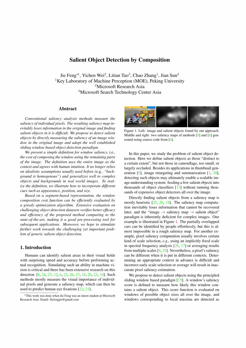
Figure 1. Left: image and salient objects found by our approach.

Middle and right: two saliency maps of methods [8] and [6] gen-

erated using source code from [6].

In this paper, we study the problem of salient object de-

tection. Here we define salient objects as those “distinct to

a certain extent”, but not those in camouflage, too small, or

largely occluded. Besides its applications in thumbnail gen-

eration [9], image retargeting and summarization [3, 20],

detecting such objects may ultimately enable a scalable im-

age understanding system: feeding a few salient objects into

thousands of object classifiers [13] without running thou-

sands of expensive object detectors all over the image.

Directly finding salient objects from a saliency map is

mostly heuristic [25, 26, 18]. The saliency map computa-

tion inevitably loses information that cannot be recovered

later, and the “image → saliency map → salient object”

paradigm is inherently deficient for complex images. One

example is illustrated in Figure 1. The partially overlapped

cars can be identified by people effortlessly, but this is al-

most impossible in a rough saliency map. For another ex-

ample, pixel saliency computation usually involves certain

kind of scale selection, e.g., using an implicitly fixed scale

in spectral frequency analysis [26, 17] or averaging results

from multiple scales [8, 25]. Nevertheless, a pixel’s saliency

can be different when it is put in different contexts. Deter-

mining an appropriate context in advance is difficult and

incorrect early scale selection or average will result in inac-

curate pixel saliency estimation.

We propose to detect salient objects using the principled

sliding window based paradigm [15]. A window’s saliency

score is defined to measure how likely this window con-

tains a salient object. This score function is evaluated on

windows of possible object sizes all over the image, and

windows corresponding to local maxima are detected as

Figure 2. Example images from PASCAL VOC 07 [11] showing different kinds of salient objects and backgrounds. Our detections (yellow)

and ground truth objects (blue) are superimposed.

salient objects. Such a detector works on the original im-

age, searches the entire image window space, and is more

likely to succeed than using an intermediate saliency map.

The key of success in this paradigm is an appropriate ob-

ject saliency1 measure that is irrespective of object classes

and robust to background variations. Looking at the various

examples in Figure 2, in spite of large variations in objects

and backgrounds, the common property is that a salient ob-

ject not only pops up from its immediate neighborhood but

is also distinctive from other objects and the entire back-

ground. In other words, it is difficult to represent a salient

object using remainder of the image. This inspires us to de-

fine an image window’s saliency as the cost of composing

the window using the remaining parts of the image.

The “composition” based definition is the key of our ap-

proach. It does not depends on assumptions such as “back-

ground is homogeneous” or “object boundary is clear and

strong”. Such assumptions are usually excessive and too

idealistic for real world images, but typically used in previ-

ous pixel saliency methods (see Section 3.1). Arguably our

definition agrees better with human intuition and captures

the essence of “what a salient window looks like”. To make

the definition precise and computable, we propose a few

computational principles by considering appearance, posi-

tion, and size information.

The window composition is performed on millions of

windows in an image and should be fast enough. Based

on a segment-based representation, we present an efficient

algorithm that leverages fast pre-computation, incremental

updating [29] and greedy optimization. The resulting detec-

tor takes less than 2 seconds for an image. Extensive eval-

uation on challenging object detection tasks verifies better

efficacy and efficiency of the proposed method comparing

to the state-of-the-art, making it a good pre-processing tool

for subsequent applications.

Detecting generic salient objects is very challenging but

quite important for image understanding. We believe the

proposed window saliency definition and computational

principles are intuitive and general for this task. Our detec-

tor is one implementation, and we hope to stimulate more

future research along this direction.

1The terms ‘window’ and ‘object’ are sometimes used interchangeably

in this paper. This issue is discussed later in Section 6.

2. Related work

In a similar spirit to our work, the objectness measure [1]

quantifies how likely an image window contains an object

of any class. It uses several existing image saliency cues

and a novel “segment straddling” cue (capturing the closed

boundary characteristic of objects). Most cues capture the

local characteristics around the window, while our saliency

measure consider the global image as context.

The segmentation framework proposed in [19] assesses

an image segment as good if it is easy to compose from it-

self but hard from remaining parts of the image. It finds a

good object segmentation by iterative optimization from a

user provided seed point. Our approach is inspired by this

work and differs in a few important aspects. Firstly, we

study a different problem and derive computational prin-

ciples (Section 3.2) from viewpoint of saliency detection,

which do not apply to segmentation. Secondly, we do not

require a good window to compose itself and our compo-

sition is not as rigid as in [19]. Therefore, our definition

on “composition” is looser and adapts to more complex ob-

jects. Finally, our composition algorithm is much faster,

enables a generic salient object detector and benefits more

potential applications.

Local, bidirectional and global self-similarity ap-

proaches [4, 3, 22] measure similarities between image

patches and exploit their geometrical patterns for image

matching [4], image summarization [3] and object recog-

nition [22]. Self-similarity has also been used to compute a

saliency map [20, 10]. Our approach exploits self-similarity

directly for salient object detection.

A lot of work uses image segmentation to help object

detection and a thorough review is beyond the scope of

this paper. A commonly adopted approach is to use dif-

ferent parameters to generate multiple segmentations and

find promising candidate segments in between [5, 14]. Such

methods depends on the segmentation algorithm to separate

the object out with appropriate parameters, and their perfor-

mance is closely coupled with the segmentation algorithm.

3. Window Saliency Definition and Principles

We first review principles for pixel saliency computation

and their limitations. Then, we define the window saliency

and discuss the computational principles.

3.1. Principles for Pixel Saliency

In spite of significant diversity in previous methods, sev-

eral principles are commonly adopted.

Local contrast/complexity principle It assumes that

high contrast or complexity of local structures indicates

high saliency. Such local measurements include various

filter responses (e.g., edge contrast [25], center-surround

difference [8, 25], curvature [18]) and several information-

theoretical measures (e.g., entropy [24], self informa-

tion [12], center-surround discriminative power [2]). This

principle works well for homogenous background and finds

accurate salient object boundaries, but does not hold for

clutter background and uniform object inside.

Global rarity principle It considers features that are

less frequent more salient. This principle agrees better

with human intuition and has been implemented in differ-

ent ways. Frequency based methods perform analysis in the

spectral domain [26, 17] and assume a low frequency back-

ground. In [25], low spatial variance of a feature is con-

sidered to indicate high saliency, and this makes an overly

strict assumption that the background everywhere is dissim-

ilar to the object. In [20], K nearest neighbors are used to

measure the saliency of an image patch.

Both local and global principles involve the difficult

early scale selection problem. To compute center-surround

measurements [8, 25, 2], a pixel neighborhood needs to be

defined. In [20], choosing a K is equal to choosing an object

scale, while an appropriate K varies among different images

or even different objects in the same image.

Priors and learning based It is often taken as a prior

that image center is more important, e.g., regulating the

saliency map with a gaussian map [25] or using the dis-

tance from center as a discriminative feature [23]. Learning

based methods are proposed to learn combination weights

of different features [25], or directly learn the saliency map

from image features [23] or by similar image retrieval from

a database [9].

3.2. Window Saliency By Composition

Observing that the salient objects are difficult to repre-

sent by the other parts of the image, and a window contain-

ing background or repeatedly occurring objects is easier to

represent, we define an image window’s saliency as the cost

of composing the window using the remaining parts of the

image. This definition subsumes the global rarity principle

and extends it from pixel to window. Note that measuring

the rarity of the window using rigid template matching is

not good because there are too many windows which can-

not find a good match in the image.

We represent an image window as a set of parts (e.g.,

patch or region) inside it, {pi}, and represent the remainder

of the image as parts outside, {po}. Composing the window

by parts provides a flexible and effective way to measure

the rarity. It allows partial matching and uses the ensemble

of all parts as the measurement. To make the composition

concept computable, we propose the following principles:

1. Appearance proximity. For po’s that are equally distant

from some pi, those more similar have a smaller com-

position cost. Using similar parts for composition sup-

presses the background and multiple similar objects.

2. Spatial proximity. For po’s that are equally similar

to some pi, those nearer have a smaller composition

cost. This makes an object further away from its simi-

lar counterparts more salient.

3. Non-Reusability. A part po can be used only once.

Otherwise a salient object can be easily composed by

a single similar background part, which is sensitive to

background clutters.

4. Non-Scale-Bias. The composition cost should be nor-

malized by window size to avoid bias towards large

windows. Thus, a tight bounding box of an object is

more salient than a loose one that contains both the

object and partial background.

These principles reflect our common perceptions about

salient objects. In experiments we found that each of them

contributes to the performance of our detector.

Image boundary regions are often partially cropped

background scenes, such as a piece of sky or grass. The

proposed definition tends to incorrectly treat such regions

as salient objects. This is addressed by replicating and ex-

tending the image boundary such that near boundary back-

ground regions can be composed from the “virtual” ex-

tended parts. It can be viewed as an “attenuate boundary”

prior, which is more general than the “favor center” prior.

4. Segment-based Composition

Given an image window, the composition problem is de-

fined as finding optimal outside parts of the same area as the

window, following the principles in Section 3.2. We present

an efficient and effective optimization algorithm that lever-

ages a segment-based representation, fast pre-computing

and incremental updating [29].

Segment-based representation is widely used in vision

tasks because it is compact and informative. We use graph-

based algorithm in [16] as it is simple and fast. We found

our results are insensitive to different parameter values. In

experiment, we use σ = 0.5,K = 250.

For two segments p and q, their appearance distance

da(p, q) is the intersection distance between their LABcolor histograms, and their spatial distance ds(p, q) is Haus-

dorff distance normalized by the longer image dimension

1

is

3

is

5

os

2

is

8

os

1

os

3

os

4

os

6

os 7

os

9

os

10

os

2

os

W

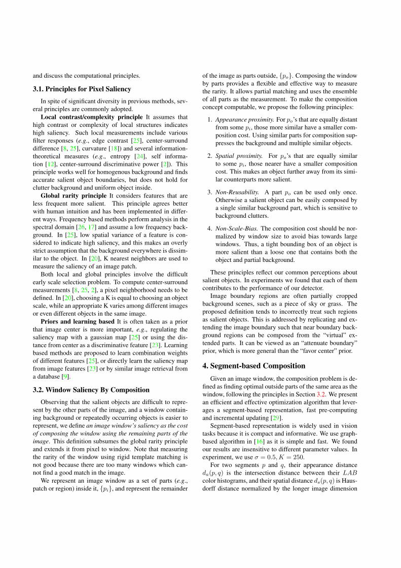
Figure 3. Illustration of segment-based composition of window

W . The inside segments are {sni |n = 1, 2, 3} and outside seg-

ments are {sno |n = 1, ..., 10}.

and clipped to [0, 1]. Their composition cost is defined as

c(p, q) = [1− ds(p, q)] · da(p, q) + ds(p, q) · dmax

a , (1)

where dmaxa is the largest appearance distance in the im-

age. The composition cost is a linear combination of their

appearance distance and maximum appearance distance,

weighted by their spatial distance. Therefore, it is monoton-

ically increasing with respect to both appearance and spatial

distances (principle 1 and 2). Note that all above pair-wise

distances are pre-computed only once.

Greedy optimization As illustrated in Figure 3, given

a window, each segment is categorized as inside if its area

within the window is larger than its area outside. Otherwise

it is categorized as outside. Composing inside segments

using outside segments can be formulated as a transporta-

tion problem, using segment areas as masses and Eq.(1) as

ground distance. However, the optimal solution, so-called

Earth Mover’s Distance [28], is very expensive to compute

and therefore infeasible.

We developed a greedy optimization algorithm that per-

forms progressive composition. Firstly, a segment strad-

dling the window boundary composes itself (without any

cost, according to Eq. (1)), i.e., its outside and inside ar-

eas cancel out as much as possible. Apparently, the more

a segment is split by the window boundary, the easier it is

composed by itself and the less salient it is. It is easy to

show that such self-composition generalizes the most effec-

tive “segment straddling” cue in objectness measure [1].

After self-composition, we define a segment’s active

area as the number of pixels not yet composed if it is in-

side, or as the number of pixels not yet used for composi-

tion if it is outside. Active area of a segment is initialized as

the difference between its inside and outside areas, and it is

updated during composition (principle 3).

Given inside/outside segments and their initial active ar-

eas, the composition algorithm is illustrated in Figure 4. It

composes the inside segments one by one (line 3), accumu-

lates the composition cost (line 7 and 16) and then normal-

izes it by window area (line 19, principle 4). To minimize

Input: an image window W , inside/outside segments {si}/{so}A(p): initial active area of segment pL(p): pre-computed list of all segments in ascending order of

their composition costs to segment pOutput: cost of composing {si} using {so}

1: cost = 02: sort {si} in descending order of their centroid to window

center’s distance

3: for each p ∈ {si}4: for each q ∈ L(p)5: if q ∈ {so} and A(q) > 06: composed area = min(A(p), A(q))7: cost← cost+ c(p, q) ∗ composed area8: A(p)← A(p)− composed area9: A(q)← A(q)− composed area

10: if A(p) = 012: break

12: end if

13: end if

14: end for

15: if A(p) > 016: cost← cost+ dmax

a ∗A(p)17: end if

18: end for

19: return cost/|W |

Figure 4. Segment-based window composition algorithm.

overall cost, inside segments that are easier to compose need

to be processed first (principle 3). Noticing that the window

center is more likely to be object (difficult to compose) and

boundary is more likely to be background (easy to com-

pose), we sort inside segments in descending order of their

distances to the window center (line 2). This ordering is

found better than other orderings we have tried (e.g., order-

ing by area).

For each inside segment p, remaining outside ones with

smaller composition costs are used at first. This is effi-

ciently implemented in two steps. In the pre-processing

step, a sorted list L(p) is created to keep all the segments

in ascending order of their composition cost with respect to

p. In the composition step, we traverse the list L(p) (line

4) but only use outside segments therein (line 5). Each out-

side segment composes p as much as possible (line 6 and

7), and their active areas are updated (line 8 and 9). Traver-

sal of L(p) is terminated when either p is totally composed

(line 10) or no outside segment remains. In the latter case,

remaining area in p is composed at maximum cost (line 16).

Because of the double loop, the worst complexity is

quadratic in the number of segments. In practice, the av-

erage complexity is much smaller as the outer loop usually

has a small number of inside segments and the inner loop

usually quickly ends after traversing the first few segments.

Efficient initialization For each window, we need to

compute its intersection areas of all segments and therefore

initial active areas. Although this can be done using integral

images in a similar way as in [1], it is still expensive due

to the linear complexity of all segments and also memory

demanding because each segment requires an integral im-

age. When a sliding window is used, it is easy to show that

such areas can be incrementally computed using the sparse

histogram representation as in [29] by treating segments as

histogram bins. We found the incremental approach is much

faster and more memory efficient.

To suppress the boundary regions as discussed in Sec-

tion 3.2, each region adjacent to the image boundary is vir-

tually extended by multiplying its area by a factor 1 + α.

Therefore more boundary regions can be composed by the

increased area. We set α as the ratio between the number of

boundary pixels and the perimeter of the segment, based on

the observation that regions closer to the boundary (larger

α) are more likely to be background. Such boundary sup-

pression is found useful in experiments.

5. Experiments

Real world images usually contain various salient ob-

jects on complex backgrounds, which is challenging for

conventional pixel saliency methods that rely on idealistic

assumptions (see discussions in Section 3.1). As our goal is

generic salient object detection with such challenges, there

is no previous work or standard dataset towards this pur-

pose, up to our knowledge.

Given this context, we choose to use standard PASCAL

VOC 07 dataset [11] for our evaluation. The dataset in-

cludes 20 object classes with a wide range of appearances,

shapes and scales. Most images contain multiple objects

on cluttered backgrounds. Note that the dataset is not en-

tirely suitable for salient object detection, because some an-

notated objects are not salient (small or partially occluded)

and some salient objects are not annotated. Nevertheless,

it is still the best public dataset for our purpose and it is

also used in [1]. Firstly, most annotated objects in it are in-

deed salient. Moreover, the large variation presents the real

world challenges and it can test the generalization ability of

a saliency algorithm and push forward research in this field.

The objectness measure [1] is the only previous work

similar to ours (see Section 2) and we mainly compare our

method to it. Note that the objectness measure is not used

as an object detector in [1] because it is too expensive to

compute for all windows. In our experiment, we use the

source code with the same parameters as in [1] to compute

all windows in a brute force manner.

Evaluation on PASCAL Our window saliency measure

and objectness [1] are evaluated over multiple sliding win-

dows. We use 7 aspect ratios (from 1:2 to 2:1) and 6 win-

dow sizes (from 2% to 50% of the image area) to cover

0 0.1 0.2 0.3 0.4 0.5 0.6 0.70

0.1

0.2

0.3

0.4

0.5

recall

pre

cis

ion

ours AP 0.183

objectness AP 0.081

Figure 5. Precision-recall curves and APs of our detector and ob-

jectness [1] based detector on PASCAL VOC 07 [11].

most object sizes, resulting in about 40 windows sizes 2.

Windows corresponding to local maxima are found by non-

maximum suppression (NMS), i.e., given all possible win-

dows, any one that is significantly overlap with another one

(intersection-over-union> θnms) with a higher score is not

locally maximal and removed. Such removal is performed

from windows with lower scores at first. The remaining

windows are detected objects.

A detected window is correct if it intersects with a

ground truth object by more than half of their union (PAS-

CAL criteria). Precision is the percentage of correctly de-

tected windows3 and recall is the percentage of ground truth

objects covered by detected windows. Detection perfor-

mance is evaluated by 1) precision-recall curves, gener-

ated by varying the score threshold and 2) average preci-

sion (AP), computed by averaging multiple precisions cor-

responding to different recalls at regular internals.

Figure 5 illustrates the performance of the two detectors

on the test set. Our saliency measure outperforms object-

ness [1] and is much better at high precision area. Because

most cues in objectness [1] are local, it can find windows

that are locally salient but globally not, such as those on

the road, horse or grass as shown in Figure 6. Our approach

takes the whole image as context and does not consider such

areas salient. Figure 7 shows more of our results on differ-

ent object and background types, and illustrates the gener-

alization ability of our approach.

Note that the evaluation results in [1] on PASCAL VOC

07 cannot be compared to those in Figure 5. In our ex-

periment, we only evaluate local optimal windows obtained

by non-maximum suppression (NMS), like most object de-

tectors. By contrast, [1] evaluates 1000 sampled windows

without NMS. See [1] for details. This is well recognized

2Typically a few of the 42 window sizes has an invalid dimension larger

than the image dimension.3This allows multiple detections for one ground truth object. It is looser

than PASCAL criteria, which only allows one detection for one object.

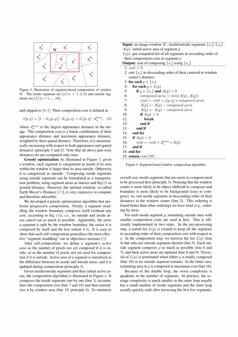
Figure 6. (best viewed in color) Example detection results on PASCAL VOC 07 using our detector(above) and objectness [1] based

detector(below). On each image the best 5 detected windows are superimposed. Yellow solid: correct detection. Red dash: wrong

detection. Blue solid: ground truth covered by correct detection.

Figure 7. (best viewed in color) Examples of our detection results on PASCAL VOC 07. On each image the best 5 detected windows are

superimposed. Yellow solid: correct detection. Red dash: wrong detection. Blue solid: ground truth covered by correct detection.

θnms 0.4 0.5 0.6 0.7 0.8

AP of objectness 0.048 0.055 0.081 0.086 0.089

AP of ours 0.142 0.157 0.183 0.191 0.198

our max recall 0.304 0.415 0.672 0.696 0.704

Table 2. APs of our detector and objectness [1] based detector, and

maximum recall of our approach using different θnms.

inappropriate for object detection evaluation [11, 15]. For

example, multiple highly overlapping windows of the same

object may be counted as correct many times.

Performance on individual object classes is evaluated on

object instances and images of a specific class. Table 1

shows that our approach outperforms objectness [1] on all

20 classes. Interestingly, the amount of improvement varies

a lot between classes and this may indicate their relative dif-

ficulties in this dataset.

Comparison to other baselines We also tested simple

baseline detectors on PASCAL using various saliency map

methods [25, 6, 17, 18, 26], where a window’s saliency is

computed as the average pixel saliency in it. All such base-

line detectors perform much worse than both objectness [1]

and our approach. It has been shown in [1] that the object-

ness measure outperforms several heuristic baselines using

saliency cues in [25, 26] and interest points. Therefore, our

approach indirectly outperforms those baselines.

Effect of NMS Parameter θnms controls the amount of

non-maximum suppression. Using an aggressive value, e.g.,

0.5, is reasonable for detecting objects of the same class

because two objects of the same class cannot overlap too

much. However, this is no longer appropriate for detecting

salient objects of different classes because they can over-

lap a lot. For example, an entire human body (with face

and legs) and the torso can be detected simultaneously, and

removing either of them appears incorrect. We tried differ-

aeroplane bicycle bird boat bottle bus car cat chair cow

objectness 0.053 0.055 0.059 0.048 0.006 0.113 0.092 0.111 0.018 0.073

ours 0.236 0.078 0.202 0.092 0.098 0.264 0.233 0.274 0.110 0.146

table dog horse motorbike person plant sheep sofa train tv

objectness 0.072 0.102 0.105 0.127 0.039 0.022 0.102 0.053 0.096 0.105

ours 0.104 0.245 0.173 0.188 0.146 0.086 0.187 0.195 0.225 0.209

Table 1. APs of our detector and objectness [1] based detector on all object classes in PASCAL VOC 07 [11]. Our approach performs

better on all object classes. The five classes improved most by our approach are highlighted.

ent values for θnms and summarize the results in Table 2.

APs and maximum recall steadily increases as θnms be-

comes looser, at the cost of generating more detected win-

dows and higher complexities for subsequent tasks. We find

θnms = 0.6 is a good trade-off and use it for all the results

in this paper.

Running time Running time of our approach depends on

the number of image segments. It is found to vary between

60 and 150 in our experiments. The pre-processing (seg-

mentation, distance computation and sorting) takes from

0.1 to 0.3 seconds. Running our detector on about 40 slid-

ing windows takes from 1 to 2 seconds on a 3G Hz CPU,

4G Mem desktop. On average, our detector takes less than

2 seconds for an image4. By contrast, the objectness [1]

based detector takes a few dozens of seconds for an image.

Though it is implemented in Matlab, we can safely conclude

that our detector is faster by a magnitude.

Single Salient Object Detection MSRA salient object

dataset [25] is less challenging because most images contain

a large object on a simple background. We present our result

on this dataset for completeness. The best window from our

detector is considered as detected salient object. Figure 8

shows a few example results.

As proposed in [25] and followed up, performance on

this dataset is evaluated by pixel level precision|O∩G||O| and

recall|O∩G||G| , where O is the detected object and G is the

ground truth object. Table 3 summarizes the performance

of our detector and other methods. Our method is compa-

rable with the state of the art [25, 18, 9]. While all other

methods use only low level features, method in [9] exploits

high level information (training and similar image retrieval

on a large database) and performs slightly better at much

higher computational cost. As many methods perform sim-

ilarly well with quite different features and approaches, this

indicates that this dataset is not challenging enough and has

been saturated to measure further progress.

It is worth noting that our method does not benefit from

the simplicity of the dataset as much as others. Our ap-

proach is principled to detect multiple objects and does not

exploit the “only one object” prior. By contrast, other meth-

4In the pre-processing, an image is firstly normalized to have its longer

dimension equal to 300.

precision recall F-measure

ours 0.82 0.82 0.82

method in [27] 0.54 0.93 0.62

method in [8] 0.66 0.82 0.68

method in [25] 0.82 0.82 0.82

method in [18] 0.85 0.76 0.79

method in [9] 0.83 0.87 0.85

Table 3. Pixel level precision, recall and F-measure of several

methods on the MSRA dataset [25]. The measure numbers of

other methods are from [25, 18]. The F-measure is computed as

in [25] (higher is better).

Figure 8. Our detection results on the MSRA dataset [25]. Yellow:

our best detection window. Blue: ground truth.

ods explicitly search the object using complex methods that

are hard to generalize for multiple objects, e.g., methods in

[25, 9] rely on an object-background binary segmentation

and method in [18] performs efficient sub-window search.

Also method in [9] requires intensive training and it is hard

to extend to multiple object classes.

6. Discussions

Finding salient objects in an image can facilitate high

level applications such as object level image matching and

retrieval. While running multiple object class detectors over

the image is too slow, it is much more efficient to run detec-

tors only around salient windows, as verified in [1]. Table 4

shows the number of detected windows and corresponding

recalls of our detector on PASCAL. The best 5 windows

cover 25% of the objects while 50% of the objects are cov-

ered by the best 30 windows. The reasonable recall, small

number of detections and high efficiency make our detector

a practical pre-processing tool for subsequent tasks.

Our approach does not exploit any high level information

and it therefore does not really model the semantics of “ob-

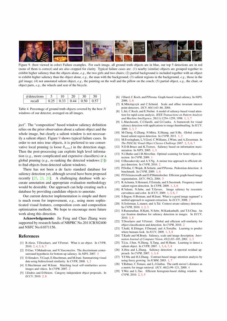
Figure 9. (best viewed in color) Failure examples. For each image, all ground truth objects are in blue, our top 5 detections are in red

(none of them is correct) and are also cropped for clarity. Typical failure cases are: (1) nearby (similar) objects are grouped together to

exhibit higher saliency than the objects alone, e.g., the two girls and two chairs; (2) partial background is included together with an object

to exhibit higher saliency than the object alone, e.g., the man with the background; (3) salient regions in the background, e.g., those in the

girl image; (4) not annotated salient object, e.g., the painting on the wall and the pillow on the couch; (5) partial object, e.g., the chair, or

object parts, e.g., the wheels and seat of the bicycle.

#detections 5 10 20 30 50

recall 0.25 0.33 0.44 0.50 0.57

Table 4. Percentage of ground truth objects covered by the best N

windows of our detector, averaged on all images.

ject”. The “composition” based window saliency definition

relies on the prior observation about a salient object and the

whole image, but clearly a salient window is not necessar-

ily a salient object. Figure 9 shows typical failure cases. In

order to not miss true objects, it is preferred to use conser-

vative local pruning (a loose θnms) in the detection stage.

Then the post-processing can exploits high level informa-

tion (e.g., more complicated and expensive classifiers) or a

global pruning (e.g., re-ranking the detected windows [5])

to find objects from detected salient windows.

There has not been a de facto standard database for

saliency detection yet, although several have been proposed

recently [25, 23, 21]. A challenging database with ac-

curate annotation and appropriate evaluation methodology

would be desirable. Our approach can help creating such a

database by providing candidate objects to annotate.

Our current detector implementation is simple and there

is much room for improvement, e.g., using more sophis-

ticated visual features, composition costs and composition

optimization methods. We hope to encourage more future

work along this direction.

Acknowledgements: Jie Feng and Chao Zhang were

supported by research funds of NBPRC No.2011CB302400

and NSFC No.61071156.

References

[1] B.Alexe, T.Deselaers, and V.Ferrari. What is an object. In CVPR,

2010. 2, 4, 5, 6, 7

[2] D.Gao, V.Mahadevan, and N.Vasconcelos. The discriminant center-

surround hypothesis for bottom-up saliency. In NIPS, 2007. 3

[3] D.Simakov, Y.Caspi, E.Shechtman, and M.Irani. Summarizing visual

data using bidirectional similarity. In CVPR, 2008. 1, 2

[4] E.Shechtman and M.Irani. Matching local self-similarities across

images and videos. In CVPR, 2007. 2

[5] I.Endres and D.Hoiem. Category independent object proposals. In

ECCV, 2010. 2, 8

[6] J.Harel, C.Koch, and P.Perona. Graph-based visual saliency. In NIPS,

2006. 1, 6

[7] K.Mikolajczyk and C.Schmid. Scale and affine invariant interest

point detectors. IJCV, 60(1):63–86, 2004.

[8] L.Itti, C.Koch, and E.Niebur. A model of saliency-based visual atten-

tion for rapid scene analysis. IEEE Transactions on Pattern Analysis

and Machine Intelligence, 20(11):1254–1259, 1998. 1, 3, 7

[9] L.Marchesotti, C.Cifarelli, and G.Csurka. A framework for visual

saliency detection with applications to image thumbnailing. In ICCV,

2009. 1, 3, 7

[10] M.Cheng, G.Zhang, N.Mitra, X.Huang, and S.Hu. Global contrast

based salient region detection. In CVPR, 2011. 1, 2

[11] M.Everingham, L.V.Gool, C.Williams, J.Winn, and A.Zisserman. In

The PASCAL Visual Object Classes Challenge 2007. 2, 5, 6, 7

[12] N.D.B.Bruce and K.Tsotsos. Saliency based on information maxi-

mization. In NIPS, 2005. 1, 3

[13] N.J.Butko and J.R.Movellan. Optimal scanning for faster object de-

tection. In CVPR, 2009. 1

[14] O.Russakovsky and A.Y.Ng. A steiner tree approach to efficient ob-

ject detection. In CVPR, 2010. 2

[15] P.Dollar, C.Wojek, B.Schiele, and P.Perona. Pedestrian detection: A

benchmark. In CVPR, 2009. 1, 6

[16] P.F.Felzenszwalb and D.P.Huttenlocher. Efficient graph-based image

segmentation. IJCV, 59(2), 2004. 3

[17] R.Achanta, S.Hemami, F.Estrada, and S.Susstrunk. Frequency-tuned

salient region detection. In CVPR, 2009. 1, 3, 6

[18] R.Valenti, N.Sebe, and T.Gevers. Image saliency by isocentric

curvedness and color. In ICCV, 2009. 1, 3, 6, 7

[19] S.Bagon, O.Boiman, and M.Irani. What is a good image segment? a

unified approach to segment extraction. In ECCV, 2008. 2

[20] S.Goferman, L.manor, and A.Tal. Context-aware saliency detection.

In CVPR, 2010. 1, 2, 3

[21] S.Ramanathan, H.Katti, N.Sebe, M.Kankanhalli, and T.S.Chua. An

eye fixation database for saliency detection in images. In ECCV,

2010. 1, 8

[22] T.Deselaers and V.Ferrari. Global and efficient self-similarity for

object classification and detection. In CVPR, 2010. 2

[23] T.Judd, K.Ehinger, F.Durand, and A.Torralba. Learning to predict

where humans look. In ICCV, 2009. 1, 3, 8

[24] T.Kadir and M.Brady. Saliency, scale and image description. Inter-

nation Journal of Computer Vision, 45(2):83–105, 2001. 1, 3

[25] T.Liu, J.Sun, N.Zheng, X.Tang, and H.Shum. Learning to detect a

salient object. In CVPR, 2007. 1, 3, 6, 7, 8

[26] X.Hou and L.Zhang. Saliency detection: A spectral residual ap-

proach. In CVPR, 2007. 1, 3, 6

[27] Y.F.Ma and H.J.Zhang. Contrast-based image attention analysis by

using fuzzy growing. In ICMM, 2003. 1, 7

[28] Y.Rubner, C.Tomasi, and L.J.Guibas. The earth mover’s distance as

a metric for image retrieval. IJCV, 40(2):99–121, 2000. 4

[29] Y.Wei and L.Tao. Efficient histogram-based sliding window. In

CVPR, 2010. 2, 3, 5