Salient features in seismic images

Salient features in seismic images

Noomane Drissi

TELECOM Bretagne- SC department

Noomane Drissi Salient features in seismic images 1/25

Outline

1 Introduction to seismic imaging

2 Saliency measure

3 Entropies

4 Tracking

5 Conclusions and perspectives


Outline


2 Saliency measure

3 Entropies

4 Tracking



Seismic imaging principle


Goals of seismic imaging

Earth structure discovery

Hydrocarbon detection

Mining applications


Use of seismic images

Detection of salient features in seismic images

Horizons

Faults

Gas chimneys...

Method : use of a saliency measure and entropies as a texturalattribute


Outline


2 Saliency measure

3 Entropies

4 Tracking



Saliency measure [Kadir 02]

Y(s, x, y) = H(s, x, y)× W(s, x, y) (1)

s is the scale and (x, y) is the pixel locationH measures the unpredictability in the feature spaceW measures the unpredictability of the feature in the scale spaceIf Y(sp, x, y) > λ, then (x, y) is a salient pixel.


Saliency measure algorithm [Kadir 02]

For every pixel1 Compute the entropy H for s ∈ [smin, smax]

2 Search for the optimal scale sp

3 Compute the inter scale measure W and the saliency Y4 Threshold


Outline


2 Saliency measure

3 Entropies

4 Tracking



Shannon Entropy

For a random variable X with a probability density function (pdf) f :

Hs(X) = −∫ ∞

−∞f (t) log f (t)dt (2)

Drawbacks:

X must have a pdf

differential entropy not always positive

nonconformity between the discrete and the continuous case


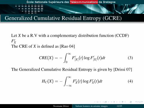
Generalized Cumulative Residual Entropy (GCRE)

Let X be a R.V with a complementary distribution function (CCDF)Fc

XThe CRE of X is defined as [Rao 04]

CRE(X) = −∫ ∞

0Fc|X|(t) log Fc

|X|(t)dt (3)

The Generalized Cumulative Residual Entropy is given by [Drissi 07]

HC(X) = −∫ ∞

−∞Fc

X(t) log FcX(t)dt (4)


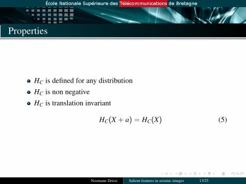
Properties

HC is defined for any distribution

HC is non negative

HC is translation invariant

HC(X + a) = HC(X) (5)


Scale invariance

For distributions with the following property:

∃µ,∀t, FcX(µ + t) = 1 − Fc

X(µ− t). (6)

we get the scale invariance property

HC(aX) = |a|HC(X), (7)


Real data

10 20 30 40 50 60 70 80 90 100

10

20

30

40

50

60

70

80

90

100


Remarks

1 Strong reflector: good detection with entropies2 Secondary reflector: better detection with Shannon entropy


Least square line

y = ax + b is the equation of the least square lineFor every threshold:(xi, yi), i = 1, .., n the coordinates of the detected pixels

Estimation of a and b


Estimation of a and b

SE GCREa b a b

Mean -0.1586 36.3139 -0.1404 35.6162Variance 1.0371e-004 0.5863 5.4257e-006 0.0512


Detection using SE (left) and using GCRE (right)

10 20 30 40 50 60 70 80 90 100

10

20

30

40

50

60

70

80

90

10010 20 30 40 50 60 70 80 90 100

10

20

30

40

50

60

70

80

90

100


Noise effect

σ2b % using HS % using HC

0 100 1000.00001 21.05 44.730.0001 13.15 36.840.001 0 31.570.01 0 21.050.1 0 5.21 0 0


Outline


2 Saliency measure

3 Entropies

4 Tracking



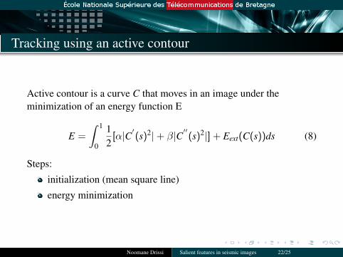
Tracking using an active contour

Active contour is a curve C that moves in an image under theminimization of an energy function E

E =

∫ 1

0

12[α|C′

(s)2|+ β|C′′(s)2|] + Eext(C(s))ds (8)

Steps:

initialization (mean square line)

energy minimization


Active contour fitting the horizon

10 20 30 40 50 60 70 80 90 100

10

20

30

40

50

60

70

80

90

100


Outline


2 Saliency measure

3 Entropies

4 Tracking



Conclusions et perspectives

1 extension of a recently introduced entropy2 application to salient features extraction in seismic images3 extraction of other seismic features and use of entropy as a

seismic attribute


Salient features in seismic images

Documents

Transcript of Salient features in seismic images