SAGEEP 2014 Refraction/Reflection Session

Optimized interpretation of SAGEEP 2011 blind refraction data with Fresnel Volume Tomography and Plus-Minus

refraction

Siegfried R.C. Rohdewald

Intelligent Resources Inc.

Vancouver, British Columbia

Canada

Smooth Inversion = 1D gradient initial model +Smooth Inversion = 1D gradient initial model +2D WET Wavepath Eikonal Traveltime tomography2D WET Wavepath Eikonal Traveltime tomography

Top : pseudo-2D DeltatV display

• 1D DeltatV velocity-depth profile below each station

• 1D Newton search for each layer• velocity too low below anticlines• velocity too high below synclines• based on synthetic times for Broad

Epikarst model (Sheehan, 2005a, Fig. 1).

Bottom : 1D-gradient initial model

• generated from top by lateral averaging of velocities

• minimum-structure initial model• DeltatV artefacts are completely

removed

Get minimum-structure 1D gradient initial model :

2D WET Wavepath Eikonal Traveltime inversion

• rays that arrive within half period of fastest ray : tSP + tPR – tSR <= 1 / 2f (Sheehan, 2005a, Fig. 2)

• nonlinear 2D optimization with steepest descent, to determine model update for one wavepath

• SIRT back-projection step, along wave paths instead of rays

• natural WET smoothing with wave paths (Schuster 1993, Watanabe 1999)

• partial modeling of finite frequency wave propagation

• partial modeling of diffraction, around low-velocity areas

• WET parameters sometimes need to be adjusted, to avoid artefacts

• see RAYFRACT.HLP help file

Fresnel volume or wave path approach :

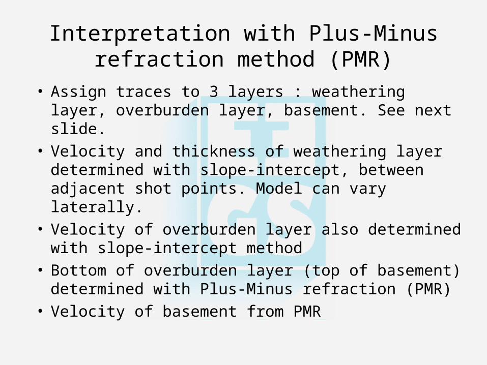
Interpretation with Plus-Minus refraction method (PMR)

• Assign traces to 3 layers : weathering layer, overburden layer, basement. See next slide.

• Velocity and thickness of weathering layer determined with slope-intercept, between adjacent shot points. Model can vary laterally.

• Velocity of overburden layer also determined with slope-intercept method

• Bottom of overburden layer (top of basement) determined with Plus-Minus refraction (PMR)

• Velocity of basement from PMR

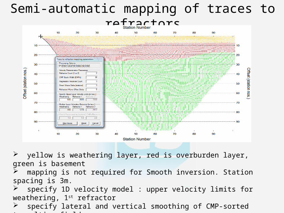
Semi-automatic mapping of traces to refractors

yellow is weathering layer, red is overburden layer, green is basement mapping is not required for Smooth inversion. Station spacing is 3m. specify 1D velocity model : upper velocity limits for weathering, 1st refractor specify lateral and vertical smoothing of CMP-sorted traveltime field map traces to refractors by matching apparent velocity to 1D velocity model lateral smoothing of crossover distance, after mapping to refractors

Plus-Minus refraction interpretation

basement velocity dips to below 2,000 m/s at station no. 63 this hints at a basement fault zone, dip of fault is not visible lateral smoothing of refractors, for Plus-Minus method (Hagedoorn, 1959) overburden refractor colored blue, basement refractor colored black

1D initial model : smooth DeltatV inversion

WET with Ricker wavelet weightingWavepath width 30%, 100 Iterations

Wavepath width 10%, 100 Iterations

Wavepath width 5%, 100 Iterations

Wavepath width 3%, 100 Iterations

050100 150 200 250 300

-60

-40

-20

0

1st run, 100 WET iters. width 30%, RMS error 0.8%, 1D-gradient starting model, smoothing 5 by 3, Version 3.25

050100 150 200 250 300

-60

-40

-20

0

1st run, 100 WET iters. width 30%, RMS error 0.8%, 1D-gradient starting model, smoothing 5 by 3, Version 3.25

050100 150 200 250 300

-60

-40

-20

0

Colin Zelt data, 100 WET iterations, RMS error 0.7 %, DeltatV initial model artefacts !, Version 3.25

050100 150 200 250 300

-60

-40

-20

0

5th run, 100 WET iters. width 5%, RMS error 0.7%, 4th run as starting model, smoothing 5 by 3, Version 3.25

WET with Gaussian weighting

050100 150 200 250 300

-60

-40

-20

0

Colin Zelt data, 100 WET iterations, RMS error 0.8 %, 1D-Gradient smooth initial model, Version 3.25

050100 150 200 250 300

-60

-40

-20

0

Colin Zelt data, 100 WET iterations, RMS error 0.7 %, DeltatV initial model artefacts !, Version 3.25

050100 150 200 250 300

-60

-40

-20

0

Colin Zelt data, 100 WET iterations, RMS error 0.7 %, DeltatV initial model artefacts !, Version 3.25

050100 150 200 250 300

-60

-40

-20

0

Colin Zelt data, 100 WET iterations, RMS error 0.6 %, DeltatV initial model artefacts !, Version 3.25

Wavepath width 30%, 100 Iterations

Wavepath width 10%, 100 Iterations

Wavepath width 5%, 100 Iterations

Wavepath width 3%, 100 Iterations

Wavepath coverage for Ricker weightingWavepath width 30%, 100 Iterations

Wavepath width 10%, 100 Iterations

Wavepath width 5%, 100 Iterations

Wavepath width 3%, 100 Iterations

050100 150 200 250 300

-60

-40

-20

0

Colin Zelt data, 100 WET iterations, RMS error 0.8 %, 1D-Gradient smooth initial model, Version 3.25

050100 150 200 250 300

-60

-40

-20

0

Colin Zelt data, 100 WET iterations, RMS error 0.7 %, DeltatV initial model artefacts !, Version 3.25

050100 150 200 250 300

-60

-40

-20

0

Colin Zelt data, 100 WET iterations, RMS error 0.7 %, DeltatV initial model artefacts !, Version 3.25

050100 150 200 250 300

-60

-40

-20

0

Colin Zelt data, 100 WET iterations, RMS error 0.6 %, DeltatV initial model artefacts !, Version 3.25

Discussion• Wide wavepaths (low frequency) make WET inversion

less dependent on the starting model and more robust but produce a smooth tomogram

• Narrow wavepaths can give a sharper tomogram, but WET becomes more dependent on the starting model (previous run) and less robust

• WET images the dipping low-velocity fault zone (Zelt et al., 2013) more realistically with iteratively decreasing wavepath width

• Contours for velocity 2,500 m/s and higher velocities become more parallel to the fault zone, which dips down to the right (towards offset 250m at elevation of -80m).

• Thin wavepaths make WET tomography more prone to generating artefacts, especially with bad or noisy first break picks and strong refractor curvature.

Conclusions• Plotting 1.5D Plus-Minus refractors on the WET

tomogram allows interactive adaptation of parameters, until the layered analysis matches the 2D velocity tomogram

• Layered refraction modeling is non-unique and subjective due to mapping of traces to assumed refractors and lateral smoothing, necessary for refractor velocity estimation and time-to-depth conversion

• WET interpretation depends on the maximum allowed basement velocity, which may not be well-constrained by the first break picks

• Gaussian weighting can produce more focused tomograms for wide wavepaths than Ricker weighting

• Tomograms obtained with an iterative approach of wavepath adjustment show improvement compared to the standard ray-based approach.