WP/07/23

SAFTA: Living in a World of Regional Trade Agreements

Jose Daniel Rodríguez-Delgado

© 2007 International Monetary Fund WP/07/23 IMF Working Paper Asia and Pacific Department

SAFTA: Living in a World of Regional Trade Agreements

Prepared by Jose Daniel Rodríguez-Delgado1

Authorized for distribution by Charles Kramer

February 2007

Abstract

This Working Paper should not be reported as representing the views of the IMF. The views expressed in this Working Paper are those of the author(s) and do not necessarily represent those of the IMF or IMF policy. Working Papers describe research in progress by the author(s) and are published to elicit comments and to further debate.

The paper evaluates the South Asia Free Trade Agreement (SAFTA) within the global structure of overlapping regional trade agreements (RTAs) using a modified gravity equation. First, it examines the effects of the Trade Liberalization Program which started in 2006. SAFTA would have a minor effect on regional trade flows and the impact on custom duties would be a manageable fiscal shock for most members. Second, the paper ranks the trade effects of other potential RTAs for individual South Asian countries and SAFTA: RTAs with North American Free Trade Agreement (NAFTA) and the European Union (EU) dominate one with the Association of South East Asian Nations (ASEAN). JEL Classification Numbers: F13, F15, F17 Keywords: SAFTA, RTAs, Trade Liberalization, South Asia Author’s E-Mail Address: jdrodrig@econ.umn.edu

1 The author was a winter intern in the IMF’s Asia and Pacific Department and a PhD candidate at the University of Minnesota when this paper was prepared. I am grateful to Sanjay Kalra for his constant guidance and encouragement and to Jerald Schiff for very valuable comments. The IMF division working on Bhutan, India, Nepal, and Sri Lanka provided a stimulating and hospitable environment.

2

Contents Page I. Introduction..........................................................................................................................3 II. SAFTA: Stylized Facts, Institutions, and Literature Review ..............................................4 III. Disentangling the Effects of SAFTA...................................................................................6 A. Theoretical Considerations ............................................................................................6 B. Model Specification and Data........................................................................................8 C. Estimation Results .......................................................................................................11 D. Simulations ..................................................................................................................11 IV. Concluding Remarks..........................................................................................................14 References................................................................................................................................23 Text Figures 1. SAFTA: Interregional Trade................................................................................................4 2. SAFTA: Average Tariffs .....................................................................................................5 3. SAFTA’s TLP Schedule ......................................................................................................7 4. SAFTA: Effects on Customs Revenue ..............................................................................12 5. Customs Revenue: Reaction to Tariffs ..............................................................................13 Text Tables 1. Distribution of SAFTA Trade Effects................................................................................11 Figures 1. South Asia: Intra-Regional Trade and Composition of Trade ...........................................16 2. SAFTA Tariffs ...................................................................................................................17 3. SA + RTAs: Regional Effects in 2004...............................................................................18 Tables 1. Gravity Equation Results ...................................................................................................19 2. South Asia and Regional Trading Arrangements ..............................................................20 Appendix 1. Selection Bias.....................................................................................................................21

3

I. INTRODUCTION

Regional trade agreements (RTAs) have emerged as an alternative to achieve trade liberalization as multilateral efforts have faced political and economic obstacles.2,3 The difficulties of reaching agreements on sensitive issues like agriculture and services have been evident in the Doha Round. The previous rounds were also marked by complex and slow negotiation processes. For one, as the number of participants increases, it has been more difficult to address each country’s demands for special considerations. RTAs convey advantages as well as limitations. By reducing the number of participants in the negotiation they can help expand the discussion to include more dimensions of economic integration. Compared with unilateral liberalization, political support for RTAs also seems to be greater given the perception of reciprocity from other member countries. However, since the early work of Viner (1950), these benefits have been weighted against distortions that RTAs can create. By de facto discriminating against nonmembers, RTAs distort resource allocation, favoring regional producers to the potential detriment of local consumers. Recent research also emphasizes the global consequences of multiple and overlapping RTAs in terms of the transaction costs they impose (Feridhanusetyawan, 2005). Although RTAs have varied components, these agreements include some or all of the following eight elements (Bhagwati and Panagariya, 1996 provide an overview): (i) a tariff liberalization program—TLP (transformation of nontariff barriers, e.g. quotas, to their tariff equivalent and the sequential reduction of tariffs; special considerations to least developed countries4 are not uncommon); (ii) sensitive lists (goods or services to be exempt from the tariff reduction program);5 (iii) rules of origin—ROO (prevention of the application of the preferential tariffs to non regional goods or services as defined by the agreement);6 (iv) institutional arrangements (establishment of a council or administrative committee responsible for the administration and implementation of the agreement); (v) trade facilitation policies (collection of instruments to reduce transaction costs of importing and

2 The literature about trade agreements is rich in acronyms that denote either their geographical extension or their degree of trade barrier reductions. RTAs refer to agreements involving regional partners. Free Trade Agreements (FTAs) refers to agreements that includes the full elimination of tariffs (and trade barriers) while Preferential Trade Agreements (PTAs) s refer to agreements involving partial tariff elimination. For example, SAPTA is South Asia’s PTA and SAFTA is South Asia’s FTA.

3 Countries could also choose to unilaterally reduce their trade barriers. In this paper we abstract from this option, although the method used here could be applied to the analysis of unilateral liberalizations.

4 United Nations (2006). In South Asia they include Bhutan, Bangladesh, Nepal, and Maldives.

5 They take the form of positive (inclusions) or negative (exclusions) lists.

6 Examples include percentage of value added in member country(ies) and specific content requirements.

4

Figure 1. SAFTA: Intra-Regional Trade(In percent of total exports and imports)

0

5

10

15

20

25

30

1988 1990 1992 1994 1996 1998 2000 2002 20040

5

10

15

20

25

30

ASEAN exports

ASEAN imports

SAFTA exports

SAFTA imports

SAPTA

Sources: COMTRADE; and author's calculations.

exporting, including homogenization of customs practices and technical assistance specially to the least-developed members); (vi) dispute settlement mechanism (procedures to report and deal with violations to the agreement); (vii) safeguards measures (suspension of preferential treatment on grounds that imports are causing or threatening to cause serious injury to the domestic industrial base); and (viii) parallel reduction in foreign investment barriers and/or trade in services. South Asia (Bangladesh, Bhutan, India, Maldives, Nepal, Pakistan and Sri Lanka) has been involved in setting up its own RTA. The South Asian Association for Regional Cooperation(SAARC) was formed in 1985 with the objective of exploiting “accelerated economic growth, social progress and cultural development in the region” for the welfare of the peoples of South Asia (SAARC Secretariat, 2006). In 1995, its corresponding RTA (SAPTA) came into force. South Asian Free Trade Agreement (SAFTA) has been ratified and entered into force in mid-2006. This paper provides a quantitative evaluation of the potential impact of SAFTA and of its possible extension to North American Free Trade Agreement (NAFTA), the European Union (EU), and Association of South East Asian Nations (ASEAN), and Plus 3.7 Section II presents an overview of trade integration in South Asia, institutional aspects of SAFTA, and existing empirical work on SAFTA. Section III details the methodology and empirical results. The paper evaluates the economic effects of trade agreements (trade flows, trade balance and customs revenue). A key result is that South Asia would obtain higher economic benefits from extending to other RTAs. However, what is true for South Asia as a bloc may not be so for each member country, generating a need for compensation mechanisms. Section IV concludes.

II. SAFTA: STYLIZED FACTS, INSTITUTIONS, AND LITERATURE REVIEW

At present, South Asia combines a low level of regional integration—especially among its largest members—and the presence of relatively high trade barriers. The proportion of trade originating in the region has increased in the last decade but still lags behind ASEAN levels. While Bangladesh, India and Pakistan sustain 5 percent of their exports and 2½ percent of their imports with regional partners, the

7 Plus 3 is used to denote the group consisting of China (including Hong Kong), Japan and Korea.

5

Figure 2. SAFTA: Average Tariffs(In percent)

0

10

20

30

40

50

1997 1998 1999 2000 2001 2002 2003 2004 20050

10

20

30

40

50Bangladesh Bhutan IndiaMaldives Nepal PakistanSri Lanka

ASEAN

Source: IMF, Trade Policy Information database.

smallest members (Bhutan, Nepal, Maldives, and Sri Lanka) exhibit a higher reliance on local trade relations averaging 20 percent and 9 percent for imports and exports, respectively.8 In terms of trade barriers the region has undertaken an overall liberalization program with India reducing its average tariff level by around 20 percentage points during the last 8 years. However, there is significant room for further liberalization given that all seven countries still impose higher tariff barriers than ASEAN and Plus3. SAPTA advanced the region’s commitment to deeper integration with limited success. The implementation of the agreement was characterized by sequential rounds of negotiations in which trade preferences were granted on a product-by-product basis. When SAPTA entered into force in December 1995, it imposed rules of origin that were too restrictive for most of its members and were subsequently lowered in 1999, and trade facilitation measures were implemented on a limited scale. Only least developed countries (LDCs) countries obtained significant trade preferences while most of the trade among the largest countries was still subject to considerable trade barriers (Baysan, and others, 2006; SAARC Secretariat, 2006c). SAFTA builds on the provisions of SAPTA. SAFTA extends the scope of SAPTA to include trade facilitation elements and switches the tariff liberalization process from a positive to a negative list approach. A special consideration in SAFTA is the compensation for revenue losses for small countries in the event of tariff reductions (Baunsgaard and Keen, 2005). For these countries SAFTA proposes that “until alternative domestic arrangements are formulated to address this situation, the Contracting States agree to establish an appropriate mechanism to compensate the Least Developed Contracting States…” (SAARC Secretariat, 2006b). SAFTA is expected to increase regional trade (trade creation) but may do so at the expense of trade flows from more efficient non regional suppliers (trade diversion). Baysan and others (2006) argue that it is unlikely that the most efficient suppliers of the member countries are within the region. Based on that and on the restrictiveness of SAFTA’s sensitive lists and rules of origin, it concludes the economic merits of SAFTA are “quite weak.” Using the static general equilibrium methodology, Bandara and Yu (2003) find that the full elimination of trade barriers between South Asian countries would increase the welfare level of India (by

8 Due to limited availability of trade statistics for smaller members, the variability should be interpreted with caution. The last observation year for these four members (exports and imports) is 1999.

6

0.2 percent) and Sri Lanka (by 0.03), but decrease the welfare level of Bangladesh ( by 0.1 percent).9 Extending the agreement to ASEAN would decrease welfare of all South Asian countries, but would increase it for an extension to NAFTA or EU (except for the rest of South Asia, which loses if it is extended toward EU). Srinivasan (1994) also forecasts the effects of SAFTA. It uses total (exports plus imports) bilateral trade flows as the dependent variable. Given data restrictions, the analysis is limited to Bangladesh, India, Nepal, Pakistan, and Sri Lanka. It concludes that Bangladesh and Nepal would gain the most from the full elimination of tariffs among South Asian members. India, Pakistan, and Sri Lanka would have only marginal benefits but would enjoy larger gains if there were a liberalization agreement with the European Economic Community.

III. DISENTANGLING THE EFFECTS OF SAFTA

A. Theoretical Considerations

Evaluating the cost and benefits of an RTA requires a quantitative framework incorporating avenues through which the agreement affects variables of interest. The literature on RTAs and trade agreements has focused on two main variables: welfare and trade flows (exports and/or imports). To establish the welfare consequences of an RTA, static general equilibrium models have been used.10 These models offer a clear and specific mapping of economic variables (e.g., welfare, GDP, employment) from the decisions of representative consumer and producer of each sector. However, their forecasting power is somewhat limited given that they use actual data from a single year called the base year (Baysan and others, 2006). To study the effects of RTAs on trade flows, typically the gravity equation approach is used. In its simplest version, it postulates a relationship between the “mass” (GDP) of two countries and their trade flows. In practical terms, the approach offers a “conditional general equilibrium” relation (Anderson and van Wincoop, 2004) in which bilateral trade is modeled as independent of trade flows with third party countries. Gravity equations have also been used to measure unobserved trade barriers, to discriminate between theoretical trade models, and to analyze the effects of trade policies (either in an ex-post or ex-ante fashion).11 The latter has been subject to critiques and refinements (e.g., Carrère, 2006) among the most important being that for the gravity equation analysis to be appropriate one needs to assume (or “condition on”) that the policy changes being

9 The GTAP database used in the paper includes Bangladesh, India, and Sri Lanka as individual countries and an aggregator named Rest of South Asia.

10 Usually denoted as CGE (Computable General Equilibrium) or GTAP. The latter denotes the use of GEMPACK programming language in the solution of the model and the source of the data. See https://www.gtap.agecon.purdue.edu/. Recent examples include World Bank (2004).

11 Anderson and van Wincoop (2004); and Feenstra, Markusen, and Rose (2001).

7

Figure 3. SAFTA's TLP Schedule 1/(In percent)

0 5 10 15 20 25 30 35

Bangladesh

Bhutan

Maldives

Nepal

Pakistan

Sri Lanka

India

Simple averageWeighted average

2008 Non-LDCs

2014 Non-LDCs 2011 LDCs

2008LDCs

Source: TRAINS; and author's calculations.1/ Latest available tariffs to other SAFTA members.

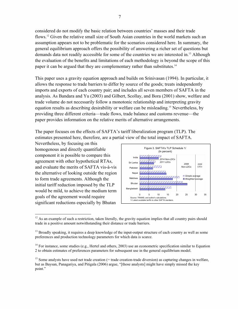
considered do not modify the basic relation between countries’ masses and their trade flows.12 Given the relative small size of South Asian countries in the world markets such an assumption appears not to be problematic for the scenarios considered here. In summary, the general equilibrium approach offers the possibility of answering a richer set of questions but demands data not readily accessible for some of the countries we are interested in.13 Although the evaluation of the benefits and limitations of each methodology is beyond the scope of this paper it can be argued that they are complementary rather than substitutes.14 This paper uses a gravity equation approach and builds on Srinivasan (1994). In particular, it allows the response to trade barriers to differ by source of the goods; treats independently imports and exports of each country pair; and includes all seven members of SAFTA in the analysis. As Bandara and Yu (2003) and Gilbert, Scollay, and Bora (2001) show, welfare and trade volume do not necessarily follow a monotonic relationship and interpreting gravity equation results as describing desirability or welfare can be misleading.15 Nevertheless, by providing three different criteria—trade flows, trade balance and customs revenue—the paper provides information on the relative merits of alternative arrangements. The paper focuses on the effects of SAFTA’s tariff liberalization program (TLP). The estimates presented here, therefore, are a partial view of the total impact of SAFTA. Nevertheless, by focusing on this homogenous and directly quantifiable component it is possible to compare this agreement with other hypothetical RTAs, and evaluate the merits of SAFTA vis-à-vis the alternative of looking outside the region to form trade agreements. Although the initial tariff reduction imposed by the TLP would be mild, to achieve the medium term goals of the agreement would require significant reductions especially by Bhutan

12 As an example of such a restriction, taken literally, the gravity equation implies that all country pairs should trade in a positive amount notwithstanding their distance or trade barriers.

13 Broadly speaking, it requires a deep knowledge of the input-output structure of each country as well as some preferences and production technology parameters for which data is scarce.

14 For instance, some studies (e.g., Hertel and others, 2003) use an econometric specification similar to Equation 2 to obtain estimates of preferences parameters for subsequent use in the general equilibrium model.

15 Some analysts have used net trade creation (= trade creation-trade diversion) as capturing changes in welfare, but as Baysan, Panagariya, and Pitigala (2006) argue, “[those analysts] might have simply missed the key point.”

8

and Maldives. In aggregate terms, the initial requirement of having tariffs lower than 30 percent by 2008 (LDCs) and 20 percent for non-LDCs would have minor effects. However, the final goal of having a tariff level of at most 5 percent will represent reductions in the average tariff rate ranging from 2 to 3 percentage points for Sri Lanka and Pakistan to 16 to 18 percentage points for Bhutan and Maldives.16

B. Model Specification and Data

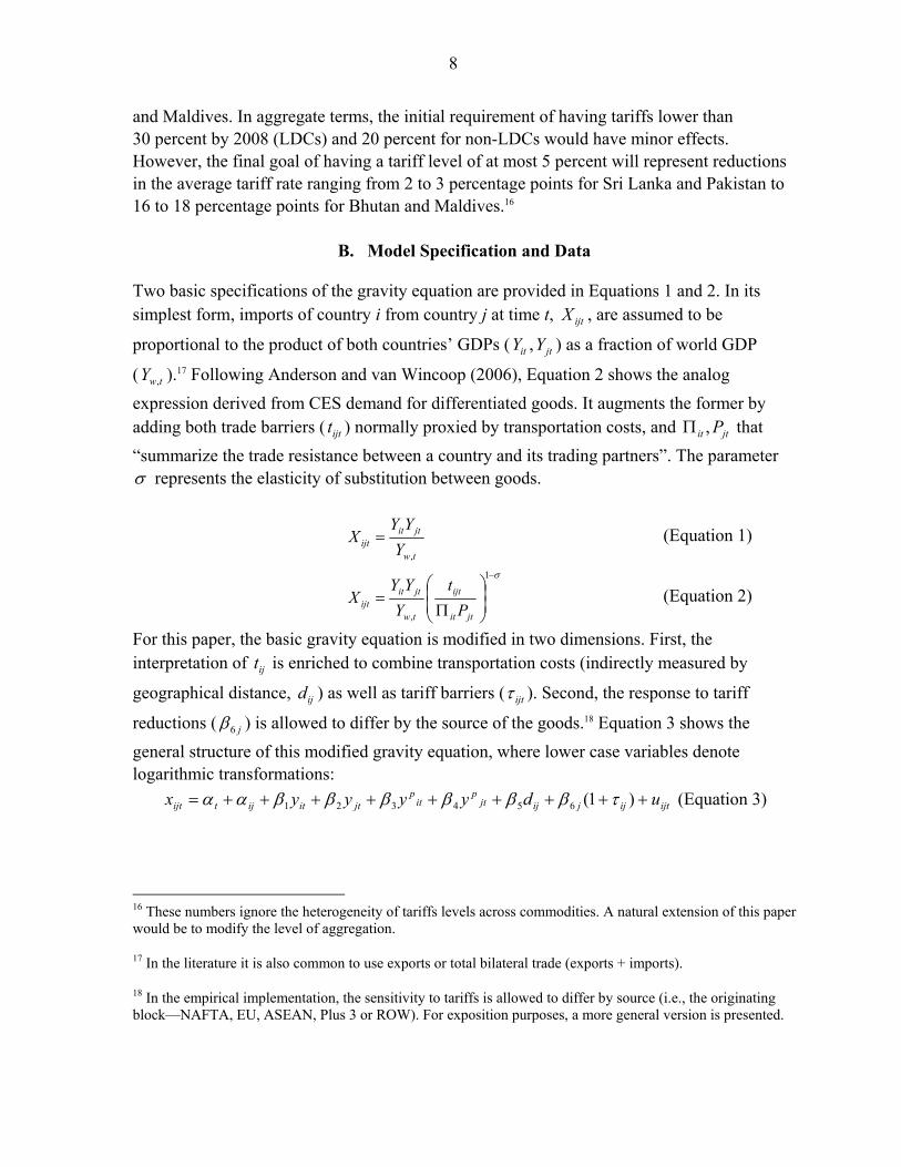
Two basic specifications of the gravity equation are provided in Equations 1 and 2. In its simplest form, imports of country i from country j at time t, ijtX , are assumed to be

proportional to the product of both countries’ GDPs ( itY , jtY ) as a fraction of world GDP

( twY , ).17 Following Anderson and van Wincoop (2006), Equation 2 shows the analog expression derived from CES demand for differentiated goods. It augments the former by adding both trade barriers ( ijtt ) normally proxied by transportation costs, and jtit P,Π that “summarize the trade resistance between a country and its trading partners”. The parameter σ represents the elasticity of substitution between goods.

tw

jtitijt Y

YYX

,

= (Equation 1)

σ−

⎟⎟⎠

⎞⎜⎜⎝

⎛

Π=

1

, jtit

ijt

tw

jtitijt P

tY

YYX (Equation 2)

For this paper, the basic gravity equation is modified in two dimensions. First, the interpretation of ijt is enriched to combine transportation costs (indirectly measured by

geographical distance, ijd ) as well as tariff barriers ( ijtτ ). Second, the response to tariff

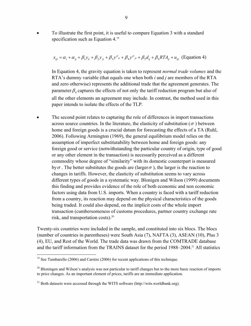
reductions ( j6β ) is allowed to differ by the source of the goods.18 Equation 3 shows the general structure of this modified gravity equation, where lower case variables denote logarithmic transformations:

ijtijjijjtp

itp

jtitijtijt udyyyyx +++++++++= )1(654321 τββββββαα (Equation 3)

16 These numbers ignore the heterogeneity of tariffs levels across commodities. A natural extension of this paper would be to modify the level of aggregation.

17 In the literature it is also common to use exports or total bilateral trade (exports + imports).

18 In the empirical implementation, the sensitivity to tariffs is allowed to differ by source (i.e., the originating block—NAFTA, EU, ASEAN, Plus 3 or ROW). For exposition purposes, a more general version is presented.

9

• To illustrate the first point, it is useful to compare Equation 3 with a standard specification such as Equation 4.19

ijtijijjt

pit

pjtitijtijt uRTAdyyyyx ++++++++= 654321 ββββββαα (Equation 4)

In Equation 4, the gravity equation is taken to represent normal trade volumes and the RTA’s dummy variable (that equals one when both i and j are members of the RTA and zero otherwise) represents the additional trade that the agreement generates. The parameter 6β captures the effects of not only the tariff reduction program but also of all the other elements an agreement may include. In contrast, the method used in this paper intends to isolate the effects of the TLP.

• The second point relates to capturing the role of differences in import transactions

across source countries. In the literature, the elasticity of substitution (σ ) between home and foreign goods is a crucial datum for forecasting the effects of a TA (Ruhl, 2006). Following Armington (1969), the general equilibrium model relies on the assumption of imperfect substitutability between home and foreign goods: any foreign good or service (notwithstanding the particular country of origin, type of good or any other element in the transaction) is necessarily perceived as a different commodity whose degree of “similarity” with its domestic counterpart is measured byσ . The better substitutes the goods are (largerσ ), the larger is the reaction to changes in tariffs. However, the elasticity of substitution seems to vary across different types of goods in a systematic way. Blonigen and Wilson (1999) documents this finding and provides evidence of the role of both economic and non economic factors using data from U.S. imports. When a country is faced with a tariff reduction from a country, its reaction may depend on the physical characteristics of the goods being traded. It could also depend, on the implicit costs of the whole import transaction (cumbersomeness of customs procedures, partner country exchange rate risk, and transportation costs).20

Twenty-six countries were included in the sample, and constituted into six blocs. The blocs (number of countries in parentheses) were South Asia (7), NAFTA (3), ASEAN (10), Plus 3 (4), EU, and Rest of the World. The trade data was drawn from the COMTRADE database and the tariff information from the TRAINS dataset for the period 1988–2004.21 All statistics 19 See Tumbarello (2006) and Carrère (2006) for recent applications of this technique.

20 Bloningen and Wilson’s analysis was not particular to tariff changes but to the more basic reaction of imports to price changes. As an important element of prices, tariffs are an immediate application.

21 Both datasets were accessed through the WITS software (http://wits.worldbank.org).

10

were used in aggregate form (1-digit SITC Rev3) where the weighted average of tariffs was constructed accordingly and the nominal variables were deflated by the U.S. GDP Deflator. Applied rather than MFN tariffs levels were used to capture actual barriers imposed on the current trade flows given that the former include existing preferential rates among countries. The use of this series has the potential of avoiding an important limitation of estimates based on dummy variables as they “do not distinguish the extent of multilateral trade liberalization” (World Bank, 2004); however, at its current stage the dataset offers an imperfect coverage of the existing RTAs (Dimaranan, 2002). As more data becomes available more refined estimates would be feasible. GDPs in nominal and per capita terms were obtained from IMF’s World Economic Outlook and World Bank’s World Development Indicators database. The distance data was obtained from Haveman (2006) or directly calculated using the great circle distance method. Although the dataset had the potential of containing 18,252 observations, information on tariffs and imports flows are prone to be infrequently reported (Anderson and van Wincoop, 2004, provides for an overview of data limitations concerning trade and trade barriers). The available number of complete observations is 3,739.22 A random effects model was estimated using standard methods to correct for endogeneity of GDP and GDP per capita in Equation 5. Such endogeneity problems have been long recognized and, as is standard in the literature, lagged values of both variables were used as instruments. As a simplifying assumption, the Rest of the World (ROW) was assumed to impose no trade barriers and to be geographically adjacent to all the countries in the sample. With this, Equation 5 implies that the final effect of a decrease in tariffs will depend on three factors: (i) the existing level of import transactions ( ijtX ); (ii) the current level of tariffs

( ijtτ+1 ); and (iii) the sensitivity of imports measured by j6β (Equation 6):

ROW} Plus3, EU, ASEAN, NAFTA, Asia,South {

)1(654321

∈

+++++++++=

k

udyyyyx ijtijkijjtp

itp

jtitijtijt τββββββαα (Equation 5)

jijt

ijtijt

ijt XX

611 βττ

∗+

∗=∂∂ (Equation 6)

where ijtX captures the standard argument in the literature that an RTA is likely to generate

more trade if it includes the main existing partners. Similarly, the presence of ijtτ+1 as a negative determinant of the trade effects can be interpreted as capturing the total effect of tariffs in the final price of imports and has the implication that one percentage point decrease in tariffs would have a larger impact for a lower initial tariff level. The notable feature of this 22 The appendix estimates a modified Equation 3 that addresses the potential effect of an unbalanced panel.

11

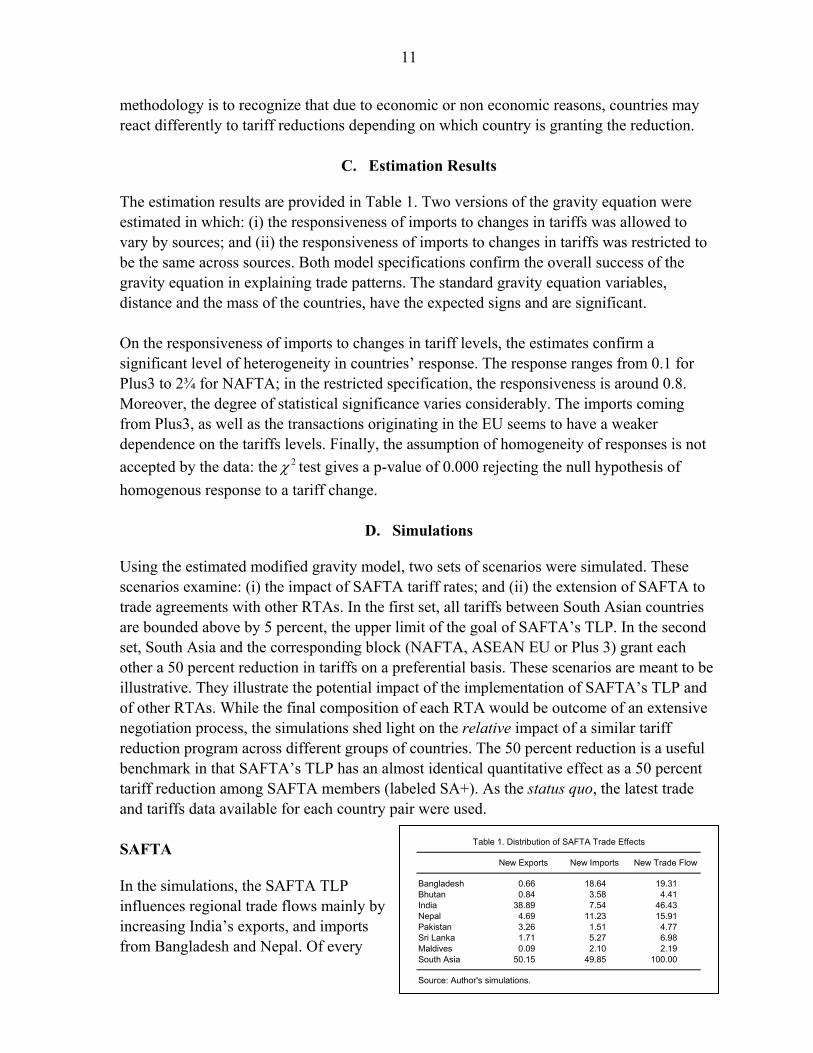
New Exports New Imports New Trade Flow

Bangladesh 0.66 18.64 19.31Bhutan 0.84 3.58 4.41India 38.89 7.54 46.43Nepal 4.69 11.23 15.91Pakistan 3.26 1.51 4.77Sri Lanka 1.71 5.27 6.98Maldives 0.09 2.10 2.19South Asia 50.15 49.85 100.00

Source: Author's simulations.

Table 1. Distribution of SAFTA Trade Effects

methodology is to recognize that due to economic or non economic reasons, countries may react differently to tariff reductions depending on which country is granting the reduction.

C. Estimation Results

The estimation results are provided in Table 1. Two versions of the gravity equation were estimated in which: (i) the responsiveness of imports to changes in tariffs was allowed to vary by sources; and (ii) the responsiveness of imports to changes in tariffs was restricted to be the same across sources. Both model specifications confirm the overall success of the gravity equation in explaining trade patterns. The standard gravity equation variables, distance and the mass of the countries, have the expected signs and are significant. On the responsiveness of imports to changes in tariff levels, the estimates confirm a significant level of heterogeneity in countries’ response. The response ranges from 0.1 for Plus3 to 2¾ for NAFTA; in the restricted specification, the responsiveness is around 0.8. Moreover, the degree of statistical significance varies considerably. The imports coming from Plus3, as well as the transactions originating in the EU seems to have a weaker dependence on the tariffs levels. Finally, the assumption of homogeneity of responses is not accepted by the data: the 2χ test gives a p-value of 0.000 rejecting the null hypothesis of homogenous response to a tariff change.

D. Simulations

Using the estimated modified gravity model, two sets of scenarios were simulated. These scenarios examine: (i) the impact of SAFTA tariff rates; and (ii) the extension of SAFTA to trade agreements with other RTAs. In the first set, all tariffs between South Asian countries are bounded above by 5 percent, the upper limit of the goal of SAFTA’s TLP. In the second set, South Asia and the corresponding block (NAFTA, ASEAN EU or Plus 3) grant each other a 50 percent reduction in tariffs on a preferential basis. These scenarios are meant to be illustrative. They illustrate the potential impact of the implementation of SAFTA’s TLP and of other RTAs. While the final composition of each RTA would be outcome of an extensive negotiation process, the simulations shed light on the relative impact of a similar tariff reduction program across different groups of countries. The 50 percent reduction is a useful benchmark in that SAFTA’s TLP has an almost identical quantitative effect as a 50 percent tariff reduction among SAFTA members (labeled SA+). As the status quo, the latest trade and tariffs data available for each country pair were used. SAFTA In the simulations, the SAFTA TLP influences regional trade flows mainly by increasing India’s exports, and imports from Bangladesh and Nepal. Of every

12

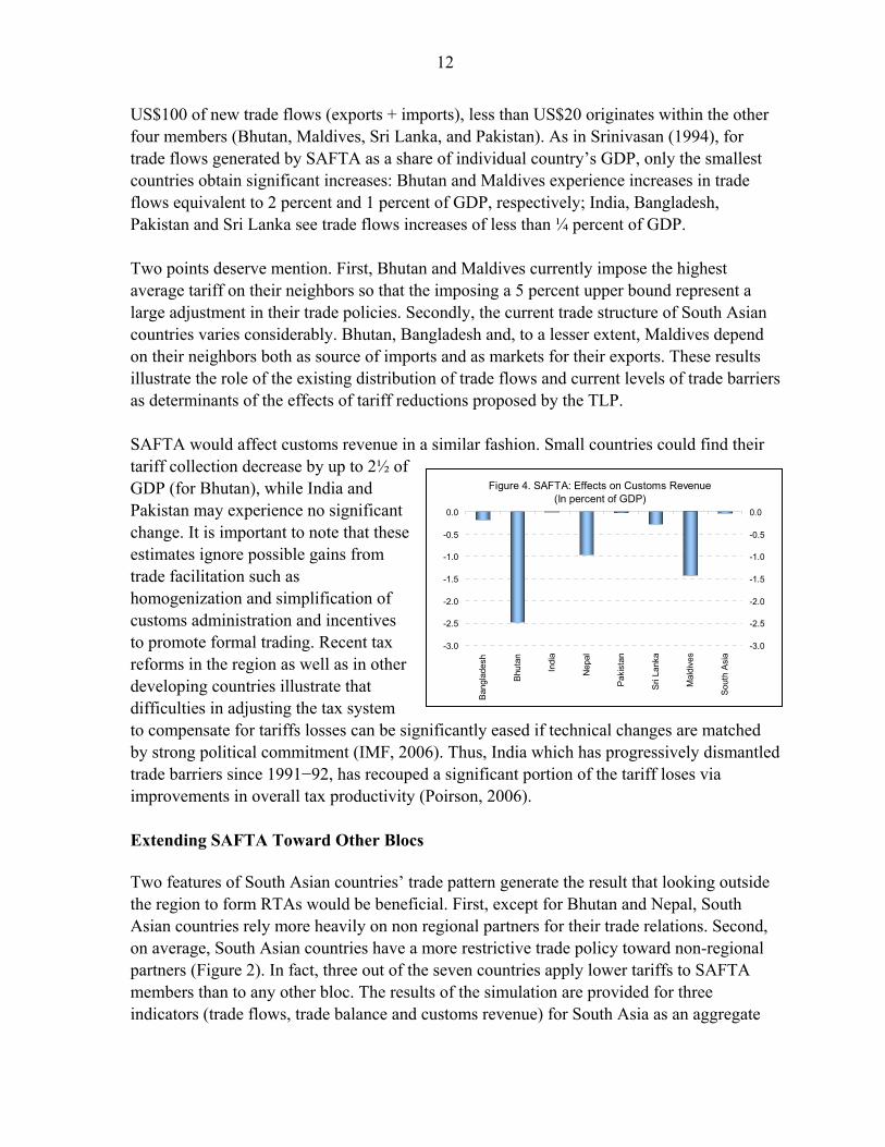
Figure 4. SAFTA: Effects on Customs Revenue(In percent of GDP)

-3.0

-2.5

-2.0

-1.5

-1.0

-0.5

0.0

Ban

glad

esh

Bhu

tan

Indi

a

Nep

al

Pak

ista

n

Sri

Lank

a

Mal

dive

s

Sout

h A

sia

-3.0

-2.5

-2.0

-1.5

-1.0

-0.5

0.0

US$100 of new trade flows (exports + imports), less than US$20 originates within the other four members (Bhutan, Maldives, Sri Lanka, and Pakistan). As in Srinivasan (1994), for trade flows generated by SAFTA as a share of individual country’s GDP, only the smallest countries obtain significant increases: Bhutan and Maldives experience increases in trade flows equivalent to 2 percent and 1 percent of GDP, respectively; India, Bangladesh, Pakistan and Sri Lanka see trade flows increases of less than ¼ percent of GDP. Two points deserve mention. First, Bhutan and Maldives currently impose the highest average tariff on their neighbors so that the imposing a 5 percent upper bound represent a large adjustment in their trade policies. Secondly, the current trade structure of South Asian countries varies considerably. Bhutan, Bangladesh and, to a lesser extent, Maldives depend on their neighbors both as source of imports and as markets for their exports. These results illustrate the role of the existing distribution of trade flows and current levels of trade barriers as determinants of the effects of tariff reductions proposed by the TLP. SAFTA would affect customs revenue in a similar fashion. Small countries could find their tariff collection decrease by up to 2½ of GDP (for Bhutan), while India and Pakistan may experience no significant change. It is important to note that these estimates ignore possible gains from trade facilitation such as homogenization and simplification of customs administration and incentives to promote formal trading. Recent tax reforms in the region as well as in other developing countries illustrate that difficulties in adjusting the tax system to compensate for tariffs losses can be significantly eased if technical changes are matched by strong political commitment (IMF, 2006). Thus, India which has progressively dismantled trade barriers since 1991−92, has recouped a significant portion of the tariff loses via improvements in overall tax productivity (Poirson, 2006). Extending SAFTA Toward Other Blocs Two features of South Asian countries’ trade pattern generate the result that looking outside the region to form RTAs would be beneficial. First, except for Bhutan and Nepal, South Asian countries rely more heavily on non regional partners for their trade relations. Second, on average, South Asian countries have a more restrictive trade policy toward non-regional partners (Figure 2). In fact, three out of the seven countries apply lower tariffs to SAFTA members than to any other bloc. The results of the simulation are provided for three indicators (trade flows, trade balance and customs revenue) for South Asia as an aggregate

13

Figure 5. Customs Revenue: Reaction to Tariffs

0

2

4

6

8

10

12

14

1 13 20 27 34 41 48 55 62 69 76 83 90 97

Tariff Level

(1+t

)/t

NAFTA = –2.77

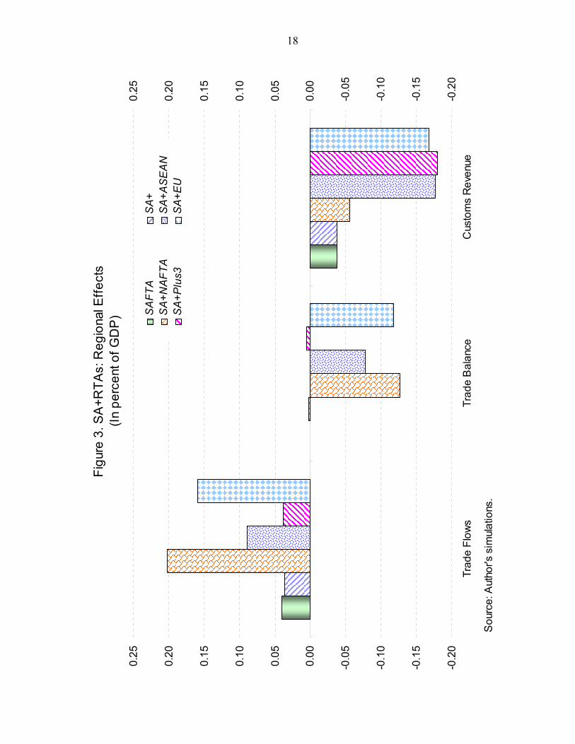
and for individual countries in South Asia. The relative attractiveness of each hypothetical RTA varies across individual countries. Trade agreements with NAFTA, EU or ASEAN would generate higher trade flows than SAFTA (Figure 3). An expansion toward ASEAN—considered to be the most natural candidate for SA further liberalization efforts (see Baysan and others, 2006)—would likely generate smaller trade flows than NAFTA or EU. Once again an important determinant is the fact that current trade relations with the European Union and NAFTA are of greater importance than bilateral flows with ASEAN members; however, an additional factor worth further exploration is the similarity between the main exports and imports of South Asia and ASEAN’s members that would make their offerings of goods and services substitutes rather than complements.23 New imports will be the driving force in all but one of these RTAs. In general most of the countries in the sample already have low tariff barriers for South Asian goods, so that the 50 percent reduction would have a minor effect in their imports (SAFTA’s exports). Furthermore, the sensitivity to South Asian tariffs ranks second to last, only larger than the corresponding to Plus 3 goods. In fact, at least 80 percent of the new trade flows from RTAs with NAFTA or EU would be in the form of new imports. In comparative terms, SA + NAFTA generates both the largest increase in trade flows and the biggest decrease in the trade balance, while SA + Plus3 shows the smallest increase in trade. Customs Revenue (CR) dynamics are determined by the level of tariffs applied to imports as well as the imports’ sensitivity to changes in such trade barriers. Equation 7 combines the definition of customs revenue with the previous decomposition of import reaction to tariffs (Equation 6). It follows that the sign of the change in revenue will be determined

by whether ττβ +

≥−1

6 j ; if that were the

case then a decrease in tariffs would in fact induce a “Laffer curve effect” increasing total custom revenues. However, even for the highly sensitive imports of NAFTA goods ( NAFTA6β = −2¾) the current level of average tariffs would have to be close to 57 percent for that phenomenon to take place, higher than any tariff currently imposed by any South Asian country. 23 Bandara and Yu (2003) use a similar argument to explain the welfare decrease that a SA + ASEAN trade agreement would have for South Asian countries.

14

⎥⎥⎦

⎤

⎢⎢⎣

⎡∗

++∗=

∂∂

+=∂∂

⇒∗= jijt

ijtijt

ijt

ijtijt

ijt

ijtijtijtijt X

XX

CRXCR 61

1)( βτ

ττ

ττ

ττ (Equation 7)

The change in customs revenue (negative in all RTAs) would likely be far from uniform. Given the strong increase in South Asian imports from NAFTA, an agreement would have the second lowest impact on customs revenue. In contrast, the apparent indifference toward changes in tariffs of Plus 3 goods supports the finding that to augment an agreement to include China, Hong Kong SAR, Japan and Korea would, on average, generate the largest custom revenue losses for the region. In sum, each of these hypothetical “extensions” of SAFTA represents a tradeoff between increasing trade flows, customs revenues, and the trade balance. SAFTA, as currently agreed, would generate the smallest loss of customs revenue but at the cost of generating the smallest expansion of trade flows. Negotiating RTAs usually involve the conciliation of differing interests of member countries and the simulations show that deciding on new trading partners is no exception (Table 2). For some of these countries (especially Bhutan and Nepal) regional trade is their main commercial channel, and SAFTA represents the highest increase in trade flows they could expect to obtain from a menu of RTAs. Maldives is an interesting case due to the unusual importance of ASEAN countries in its trade flows, and would experience the highest increase in trade flows from an expansion to this bloc. If the objective of a country was to minimize trade imbalances, SA + NAFTA would receive support from Bangladesh, Sri Lanka, and the Maldives; SAFTA would be favored by India and Pakistan. Simulations of the effects on customs revenue (with their limitations already mentioned above) provide two main conclusions: (i) SA + NAFTA would likely lead to the lowest revenue loss, except for India and Pakistan; and (ii) its effects would be heterogeneous, ranging from .01 percent of GDP for Bhutan to 0.2 percent for Maldives. Such unequal distribution of revenue effects is far form being exclusive to an agreement with NAFTA, in fact, as currently conceived, the TLP of SAFTA generates the widest range of effects.

IV. CONCLUDING REMARKS

Regional trade agreements have been, and will likely remain, an important tool for trade liberalization. While theory is skeptic about RTAs, most empirical studies find that trade creation dominates trade diversion. In practice several factors increase the benefits of RTAs, including large and diverse membership, low external most-favored-nation tariffs, comprehensiveness, liberal rules of origin, and trade facilitation measures. On these grounds, SAFTA offers room for improvement. Restrictive rules of origin, extensive sensitive lists and uncoordinated efforts currently threaten to limit the trade potential of the region. SAPTA was a clear example of the limitations of imposing restrictive rules of origin as well as of the negative role played by exclusion lists that in some cases covered the vast majority of the existing trade (Baysan, and others, 2006). The India-Sri Lanka FTA suffered similar

15

restrictions and yet has significantly increased trade between India and Sri Lanka, showing the vast potential of unexplored commercial linkages. Not all RTAs are created equal. They vary in terms of their capacity to generate additional trade, overall economic integration, and distribution of benefits among members. Focusing on the tariff reduction component of RTAs, South Asian benefits would be distributed toward the smallest countries. There is also evidence that extending SAFTA to other RTAs including NAFTA, EU, Plus 3 or ASEAN confers benefits. There are important additional gains from pursuing a coordinated approach to deeper economic integration. Some of South Asian’s members are currently pursuing individual trade agreements with NAFTA and with other Asian countries, however the added complexity of cascading trade barriers could turn this approach into a losing proposition for not only the region as a whole but also for, ironically, the very negotiating countries (World Bank 2004).

16

Figure 1. South Asia: Intra-Regional Trade and Composition of Trade

SAFTA: Intra-Regional Trade(In percent of total exports and imports)

0

10

20

30

40

50

1989 1991 1993 1995 1997 1999 2001 20030

10

20

30

40

50Group1: Imports 1/Group 2: Imports 2/Group1: Exports 1/Group2: Exports 2/

Sources: COMTRADE; and Author's calculations.1/ Bangladesh, India, and Pakistan.2/ Bhutan, Maldives, Nepal, and Sri Lanka.

SAPTA

South Asia: Trade Composition(In percent of total trade)

0%

20%

40%

60%

80%

100%

Bangladesh Bhutan India Nepal

SAFTA ASEAN EU NAFTA Plus3 ROW

South Asia: Trade Composition(In percent of total trade)

0%

20%

40%

60%

80%

100%

Pakistan Sri Lanka Maldives South Asia

SAFTA ASEAN EU NAFTA Plus3 ROW

17

Figure 2. SAFTA Tariffs

0

5

10

15

20

25

30

35

Bangladesh Bhutan India Maldives0

5

10

15

20

25

30

35

ASEAN EU NAFTA

Plus3 SAFTA

Source: TRAINS. 1/ Except for India, Pakistan, and Sri Lanka (2005).

Weighted Average of Applied Tariffs in 2004 1/(In percent)

0

5

10

15

20

25

30

35

Nepal Pakistan Sri Lanka0

5

10

15

20

25

30

35

ASEAN EU NAFTA

Plus3 SAFTA

Source: TRAINS. 1/ Except for India, Pakistan, and Sri Lanka (2005).

Weighted Average of Applied Tariffs in 2004 1/(In percent)

South Asia: Tariffs Imposed on Its Exports(Applied tariffs, weighted average)

0

5

10

15

20

25

1988 1990 1992 1994 1996 1998 2000 2002 2004

ASEAN EU

NAFTA Plus3

Sources: TRAINS; and author's calculations.

18

Figu

re 3

. SA

+RTA

s: R

egio

nal E

ffect

s(In

per

cent

of G

DP

)

-0.2

0

-0.1

5

-0.1

0

-0.0

5

0.00

0.05

0.10

0.15

0.20

0.25

Trad

e Fl

ows

Trad

e B

alan

ceC

usto

ms

Rev

enue

-0.2

0

-0.1

5

-0.1

0

-0.0

5

0.00

0.05

0.10

0.15

0.20

0.25

SA

FTA

SA

+S

A+N

AFT

AS

A+A

SE

AN

SA

+Plu

s3S

A+E

U

Sou

rce:

Aut

hor's

sim

ulat

ions

.

19

GLS-IV GLS-IVRandom Effects Random Effects

Model Unrestricted Unrestricted

Observations 3,739 3,739

R-sq 0.781 0.772

Coefficients Value P-value Value P-valueTariffs on South Asian goods -0.492 0.13 -0.813 0.00Tariffs on ASEAN goods -0.588 0.03 -0.813 0.00Tariffs on EU goods -0.885 0.27 -0.813 0.00Tariffs on NAFTA goods -2.773 0.00 -0.813 0.00Tariffs on Plus4 goods -0.106 0.78 -0.813 0.00Tariffs on ROW goods -1.720 0.09 -0.813 0.00

Gravity variablesGDP*GDP 0.887 0.00 0.885 0.00GDP per capita source -0.200 0.00 -0.233 0.00GDP per capita destination 0.351 0.00 0.309 0.00Distance -0.152 0.00 -0.154 0.00

Control variablesASEAN goodsTime dummies

Source: Author's estimates.

Table 1. Gravity Equation Results

20

SAFTA SA+ NAFTA ASEAN Plus 3 EU

Increase in trade flowsBangladesh 0.11 0.09 0.15 0.12 0.04 0.06Bhutan 2.09 1.37 0.02 0.05 0.01 0.03India 0.02 0.02 0.19 0.09 0.04 0.17Nepal 0.81 0.62 0.11 0.11 0.03 0.15Pakistan 0.02 0.01 0.27 0.06 0.06 0.10Sri Lanka 0.12 0.22 0.27 0.17 0.04 0.26Maldives 0.94 0.69 0.73 1.58 0.03 0.66SAFTA 0.04 0.04 0.20 0.09 0.04 0.16

Change in trade balanceBangladesh -0.11 -0.08 0.05 -0.12 -0.03 -0.06Bhutan -1.30 -0.74 -0.02 -0.05 -0.01 -0.03India 0.02 0.02 -0.15 -0.07 0.01 -0.12Nepal -0.33 -0.25 -0.03 -0.11 -0.03 -0.15Pakistan 0.01 0.00 -0.13 -0.05 0.01 -0.10Sri Lanka -0.06 -0.04 0.01 -0.16 -0.02 -0.13Maldives -0.86 -0.57 -0.34 -1.49 -0.03 -0.66SAFTA 0.00 0.00 -0.13 -0.08 0.00 -0.12

Change in customs revenueBangladesh -0.19 -0.19 -0.02 -0.23 -0.40 -0.07Bhutan -2.47 -2.55 -0.01 -0.08 -0.12 -0.04India -0.01 -0.01 -0.06 -0.18 -0.14 -0.18Nepal -0.98 -0.99 -0.02 -0.20 -0.32 -0.20Pakistan -0.02 -0.02 -0.07 -0.10 -0.30 -0.12Sri Lanka -0.28 -0.28 -0.05 -0.29 -0.30 -0.23Maldives -1.42 -1.45 -0.18 -2.99 -0.38 -0.84SAFTA -0.04 -0.04 -0.06 -0.18 -0.18 -0.17

Source: Author's simulations.

(In percent of GDP)

Table 2. South Asia and Regional Trading Arrangements

21

Number ofOccurrences Pairin the Sample Frequency Percent Cumulative

0 168 24.85 24.851 48 7.10 31.952 29 4.29 36.243 45 6.66 42.904 31 4.59 47.495 48 7.10 54.596 56 8.28 62.877 22 3.25 66.128 25 3.70 69.829 27 3.99 73.82

10 63 9.32 83.1411 34 5.03 88.1712 19 2.81 90.9813 2 0.30 91.2714 1 0.15 91.4215 19 2.81 94.2316 19 2.81 97.0417 20 2.96 100.00

Total 676 100.00

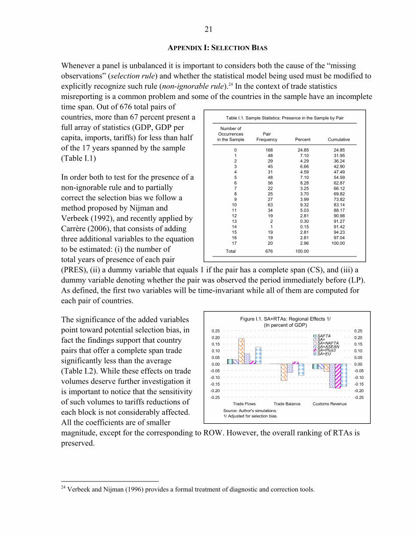
Table I.1. Sample Statistics: Presence in the Sample by Pair

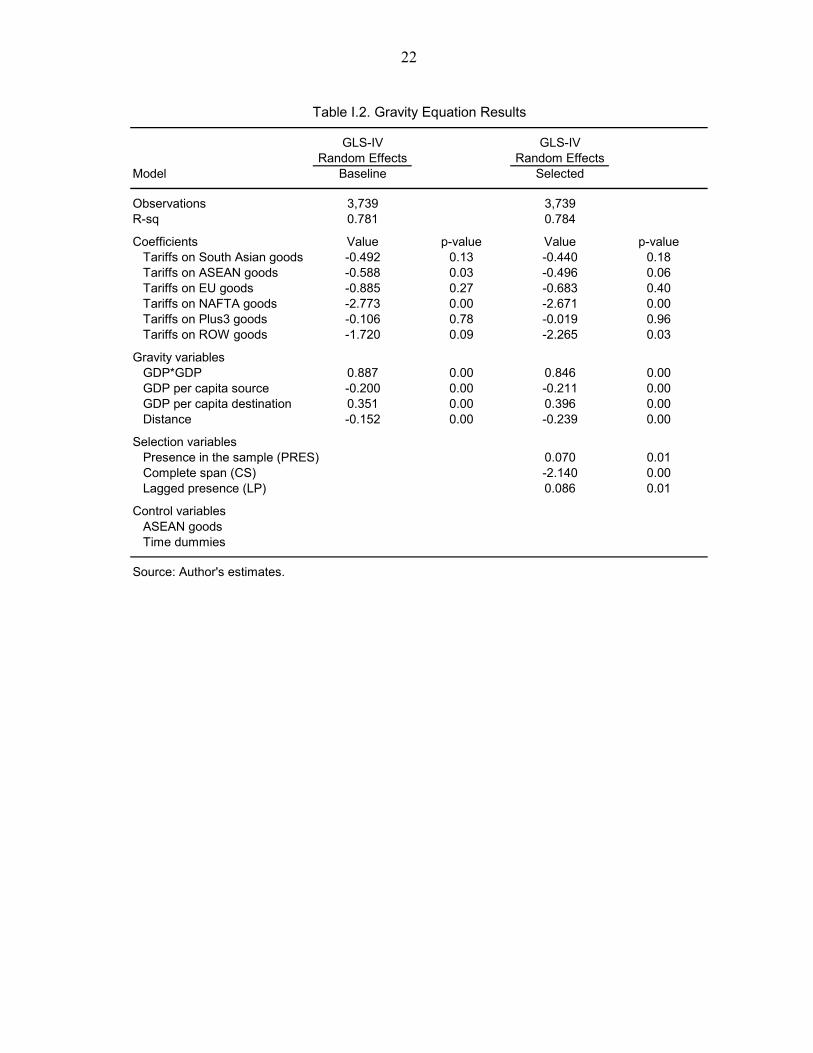
APPENDIX I: SELECTION BIAS Whenever a panel is unbalanced it is important to considers both the cause of the “missing observations” (selection rule) and whether the statistical model being used must be modified to explicitly recognize such rule (non-ignorable rule).24 In the context of trade statistics misreporting is a common problem and some of the countries in the sample have an incomplete time span. Out of 676 total pairs of countries, more than 67 percent present a full array of statistics (GDP, GDP per capita, imports, tariffs) for less than half of the 17 years spanned by the sample (Table I.1) In order both to test for the presence of a non-ignorable rule and to partially correct the selection bias we follow a method proposed by Nijman and Verbeek (1992), and recently applied by Carrère (2006), that consists of adding three additional variables to the equation to be estimated: (i) the number of total years of presence of each pair (PRES), (ii) a dummy variable that equals 1 if the pair has a complete span (CS), and (iii) a dummy variable denoting whether the pair was observed the period immediately before (LP). As defined, the first two variables will be time-invariant while all of them are computed for each pair of countries. The significance of the added variables point toward potential selection bias, in fact the findings support that country pairs that offer a complete span trade significantly less than the average (Table I.2). While these effects on trade volumes deserve further investigation it is important to notice that the sensitivity of such volumes to tariffs reductions of each block is not considerably affected. All the coefficients are of smaller magnitude, except for the corresponding to ROW. However, the overall ranking of RTAs is preserved.

24 Verbeek and Nijman (1996) provides a formal treatment of diagnostic and correction tools.

Figure I.1. SA+RTAs: Regional Effects 1/(In percent of GDP)

-0.25-0.20-0.15-0.10-0.050.000.050.100.150.200.25

Trade Flows Trade Balance Customs Revenue-0.25-0.20-0.15-0.10-0.050.000.050.100.150.200.25

SAFTASA+SA+NAFTASA+ASEANSA+Plus3SA+EU

Source: Author's simulations.1/ Adjusted for selection bias.

22

GLS-IV GLS-IVRandom Effects Random Effects

Model Baseline Selected

Observations 3,739 3,739R-sq 0.781 0.784

Coefficients Value p-value Value p-valueTariffs on South Asian goods -0.492 0.13 -0.440 0.18Tariffs on ASEAN goods -0.588 0.03 -0.496 0.06Tariffs on EU goods -0.885 0.27 -0.683 0.40Tariffs on NAFTA goods -2.773 0.00 -2.671 0.00Tariffs on Plus3 goods -0.106 0.78 -0.019 0.96Tariffs on ROW goods -1.720 0.09 -2.265 0.03

Gravity variablesGDP*GDP 0.887 0.00 0.846 0.00GDP per capita source -0.200 0.00 -0.211 0.00GDP per capita destination 0.351 0.00 0.396 0.00Distance -0.152 0.00 -0.239 0.00

Selection variablesPresence in the sample (PRES) 0.070 0.01Complete span (CS) -2.140 0.00Lagged presence (LP) 0.086 0.01

Control variablesASEAN goodsTime dummies

Source: Author's estimates.

Table I.2. Gravity Equation Results

23

References Anderson, J. E., and E. van Wincoop, 2004, “Trade Costs,” Journal of Economic Literature,

Vol. 42, No. 3, pp. 691–751. Armington, P., 1969, “A Theory of Demand for Products by Place of Production,” Staff

Papers, International Monetary Fund, Vol. 16, No. 1, pp. 170–201. Baier, S. L., and J. H. Bergstrand, 2005, “Do Free Trade Agreements Actually Increase

Member’s International Trade,” Federal Reserve Bank of Atlanta Working Paper 2005–3. Bandara, J. S., and W. Yu, 2003, “How Desirable is the South Asian Free Trade Area? A

Quantitative Assessment,” World Economy, Vol. 26, No. 9, pp. 1293–1323. Baunsgaard, T., and M. Keen, 2005, “Tax Revenue and (or?) Trade Liberalization.” IMF

Working Paper No. 05/112 (Washington: IMF). Baysan, T., A. Panagariya, and N. Pitigala, 2006, “Preferential Trading in South Asia,”

World Bank Policy Research Working Paper No. 3813 (Washington: World Bank). Bhagwati, J., and A. Panagariya, 1996, “The Theory of Preferential Trade Agreements: Historical

Evolution and Current Trends,” American Economic Review, Vol. 86, No. 2, pp. 82–87. Bloningen, B.A. and W.W. Wilson (1999), “Explaining Armington: What Determines

Substitutability between Home and Foreign Goods?” The Canadian Journal of Economics, Vol. 32, No. 1, pp. 1–21.

Carrère, C., 2006, “Revisiting the Effects of Regional Trade Agreements on Trade Flows with

Proper Specification of the Gravity Model,” European Economic Review, Vol. 50, pp. 223−47. Dimaranan, B.V., 2002, “Preferential Tariff Rates from WITS and MacMaps: Comparison

for Tariffs on Manufactured Commodities.” Available via the Internet: https://www.gtap.agecon.purdue.edu/events/Board_Meetings/2003/docs.

Economist, 2006, “Five Minutes to Midnight,” Vol. 379, Issue 8475, pp. 13–14. Feridhanusetyawan, T., 2005, “Preferential Trade Agreements in the Asia-Pacific Region,”

IMF Working Paper No. 05/149 (Washington: IMF). Feenstra, R.C., J.R. Markusen, and A.K. Rose, 2001, “Using the Gravity Equation to

Differentiate Among Alternative Theories of Trade,” Canadian Journal of Economics, Vol. 34, No. 2, pp. 430–47.

24

Gilbert, J., R. Scollay, and B. Bora, 2001, “Assessing Regional Trading Arrangements in the

Asia-Pacific,” United Nations Conference on Trade and Development, Policy Issues in International Trade and Commodities, Study Series No. 15.

Hertel, T., D. Hummels, M. Ivanic, and R. Keeney, 2003, “How Confident Can We Be in

CGE-Based Assessments of Free Trade Agreements,” GTAP Working Paper No. 26. International Monetary Fund, 2006, “Integrating Poor Countries into the World Trading

System,” Economic Issues, No. 37 (Washington: IMF). Newfarmer, R., and M.D. Piérola, 2006, “SAFTA: Promise and Pitfalls of Preferential Trade

Arrangements,” (unpublished; Washington: World Bank). Panagariya, A., 2003, “South Asia: Does Preferential Trade Liberalization Make Sense?”

World Economy, Vol. 26, No. 9, pp. 1279–291. Poirson, H., 2006, “The Tax System in India: Could Reform Spur Growth?,” IMF Working

Paper No. 06/93 (Washington: IMF). Ruhl, K. J, 2006, “The International Elasticity Puzzle,” Available via the Internet:

http://www.eco.utexas.edu/~kjr296/. SAARC Secretariat, 2006a, “A Brief on SAARC,” Available via the Internet:

http://www.saarc-sec.org. __________, 2006b, “Agreement on South Asian Free Trade Area (SAFTA).” Available via

the Internet: http://www.saarc-sec.org. __________, 2006c, “Agreement on SAARC Preferential Trading Arrangement (SAPTA)”

Available via the Internet: http://www.saarc-sec.org Srinivasan, T.N. (1994), “Regional Trading Arrangements and Beyond: Exploring Some

Policy Options for South Asia” World Bank Report No. IDP 42. Tumbarello, P., 2006, “Are Regional Trade Agreements in Asia Open or Closed Blocs?” in

Asia and Pacific Regional Outlook, May, pp. 74–78 (Washington: IMF). Varbeek, M., and T. Nijman, 1996, “Incomplete Panels and Selection Bias,” in The

Econometrics of Panel Data: A Handbook of the Theory with Applications, Second Edition , ed. by Laszlo Matyas and Patrick Sevestre.

25

Viner, J., 1950, The Customs Union Issue (New York: Carnegie Endowment for International Peace).

United Nations, 2006, “LDCs List.” Available via the Internet: http://www.un.org/. World Bank, 2004, Global Economic Prospects 2005: Trade, Regionalism and Development

(Washington: World Bank).