Safety Evaluation of Concrete Structures with Nonlinear...
118
Safety Evaluation of Concrete Structures with Nonlinear Analysis HENDRIK SCHLUNE Department of Civil and Environmental Engineering Division of Structural Engineering Concrete Structures CHALMERS UNIVERSITY OF TECHNOLOGY Gothenburg, Sweden, 2011
Transcript of Safety Evaluation of Concrete Structures with Nonlinear...

Safety Evaluation of Concrete Structures with Nonlinear Analysis
HENDRIK SCHLUNE Department of Civil and Environmental Engineering Division of Structural Engineering Concrete Structures CHALMERS UNIVERSITY OF TECHNOLOGY Gothenburg, Sweden, 2011

THESIS FOR THE DEGREE OF DOCTOR OF PHILOSOPHY
Safety Evaluation of Concrete Structures with Nonlinear Analysis
HENDRIK SCHLUNE
Department of Civil and Environmental Engineering Division of Structural Engineering
Concrete Structures CHALMERS UNIVERSITY OF TECHNOLOGY
Gothenburg, Sweden, 2011

Safety Evaluation of Concrete Structures with Nonlinear Analysis HENDRIK SCHLUNE Gothenburg, 2011 ISBN 978-91-7385-551-8
© HENDRIK SCHLUNE, 2011
Thesis for the degree of doctor of philosophy Ny serie: 3232 ISSN 0346-718X Department of Civil and Environmental Engineering Division of Structural Engineering Concrete Structures Chalmers University of Technology SE-412 96 Gothenburg Sweden Telephone: + 46 (0)31-772 1000 Cover: Photograph of the new Svinesund Bridge Chalmers Reproservice Gothenburg, Sweden, 2011


CHALMERS, Civil and Environmental Engineering I
Safety Evaluation of Concrete Structures with Nonlinear Analysis HENDRIK SCHLUNE Department of Civil and Environmental Engineering Division of Structural Engineering, Concrete Structures Chalmers University of Technology
ABSTRACT
Concrete is the most widely used construction material in the world. To obtain effective new constructions and to use existing concrete structures in an optimal way, accurate structural models are needed. This requires that good approximations of important model parameters be available and that the nonlinear material response of concrete can be accounted for.
However, uncertain model parameters can significantly influence the structural response modelled which leads to high modelling uncertainty. To estimate uncertain parameters a methodology is proposed and applied to the new Svinesund Bridge to improve the initial finite element model through finite element model updating using on-site measurements.
To account for the nonlinear material response, it is also necessary to have a safety format suited to nonlinear analysis. However, the available safety formats for nonlinear analysis have been questioned and the need to quantify the modelling uncertainty of nonlinear analysis has been highlighted, Carlsson et al. (2008).
Therefore, the modelling uncertainty of nonlinear analysis was quantified based on available data. It was found that the uncertainty varies significantly depending on the failure mode obtained and that this uncertainty was often the factor that governed the safety evaluation. Based on this observation, a new safety format is proposed which allows the modelling uncertainty be explicitly accounted for. To facilitate realistic modelling the mean in situ material parameters are used in the nonlinear analysis; the reliability is assured by a, so called, resistance safety factor. Apart from the modelling uncertainty, the resistance safety factor depends on the material and geometrical uncertainty. It was found that the material variability can be estimated by using a sensitivity study, which involves two to three additional nonlinear analyses with reduced material strengths.
Applying the safety format to short columns loaded by a normal force and to beam sections loaded in bending, shear, and the combination of bending and shear, led to a reliability level that was in good agreement with the target reliability. Other safety formats for nonlinear analysis, according to EN 1992-2, CEN (2005), and Model Code 2010, fib (2010a), fib (2010b), were found to underestimate the modelling uncertainty of difficult-to-model failure modes, leading to a reliability level below the target reliability.
To study the consequences of assuring the safety on the structural level by an inequality of forces, as proposed in Model Code 2010, four safety formats were applied to a concrete portal frame bridge. It was shown that an inequality of forces on the structural level does not necessarily lead to the intended reliability level, unless the deformation capacity used is reliably available.
Key words: nonlinear analysis; modelling uncertainty, safety format; concrete; reliability; model updating, structural identification, concrete structures
II CHALMERS, Civil and Environmental Engineering
Contents
1 INTRODUCTION 1
1.1 Background 1
1.2 Objective, scientific approach and limitations 1
1.3 Original features 2
1.4 Outline 2
2 FINITE ELEMENT MODEL UPDATING 3
2.1 Background 3
2.2 Problem description 3
2.3 Bridge evaluation by static load testing 4
2.4 FE model updating in structural dynamics 5
2.5 Proposed methodology 5
2.6 Application to the new Svinesund Bridge 6 2.6.1 The new Svinesund Bridge 6 2.6.2 Updating of the finite element model 6 2.6.3 Results of updating 7
2.7 General recommendations 8
3 SAFETY EVALUATION OF CONCRETE STRUCTURES WITH NONLINEAR ANALYSIS 11
3.1 Background 11
3.2 Reliability methods 13 3.2.1 Level III methods 14 3.2.2 Level II methods 15 3.2.3 Level I methods 15 3.2.4 Limitation of reliability methods 16
3.3 Modelling uncertainty of nonlinear analysis 17 3.3.1 Comparison of two-step and one-step procedures 17 3.3.2 Quantification of modelling uncertainty 18
3.4 Available safety formats for nonlinear analysis 19 3.4.1 The partial factor method 19 3.4.2 The global resistance factor method 21 3.4.3 The safety format according to EN 1992-2 21 3.4.4 The estimated coefficient of variation method 22 3.4.5 The safety format according to Six (2001) 23 3.4.6 The safety format according to Henriques et al. (2002) 24 3.4.7 Discussion of existing safety formats 24
3.5 Proposal of a new safety format 25 3.5.1 General outline 25 3.5.2 Structural modelling uncertainty 26
CHALMERS, Civil and Environmental Engineering III
3.5.3 Geometrical uncertainty 30 3.5.4 Material uncertainty 30
3.6 Testing of the new safety format 31 3.6.1 Resistance side 32 3.6.2 Global reliability 33 3.6.3 The portal frame bridge 35
3.7 Discussion 35 3.7.1 Deformation capacity 35 3.7.2 Human error 37 3.7.3 Verification and the one-step procedure 37
4 CONCLUSIONS 39
4.1 Finite element model updating 39 4.1.1 General conclusions 39 4.1.2 Suggestions for future research 39
4.2 Safety Evaluation of Concrete Structures with Nonlinear Analysis 39 4.2.1 General conclusions 39 4.2.2 Suggestions for future research 40
5 REFERENCES 41

IV CHALMERS, Civil and Environmental Engineering
Preface The research presented here was carried out from January 2007 until June 2011 at the Chalmers University of Technology, Department of Civil and Environmental Engineering, Division of Structural Engineering. This study was financed by the Swedish Research Council, FORMAS, and the Swedish Transport Administration, Trafikverket.
My initial plan was to study one semester of economics abroad to improve my English and to enjoy the Australian sunshine. However, due to a good personal reason the destination was changed to Gothenburg and the topic was changed to structural engineering.
The stay in Gothenburg was made possible by Silke Olmscheid from the International Office and by Professor Reinhard Maurer from the Technical University of Dortmund who supported me during the struggle with bureaucracy. The interesting lectures given by Professor Björn Engström made me extend my stay by one year to write the Master’s thesis at Chalmers under the helpful supervision of Professor Karin Lundgren and Kamyab Zandi Hanjari, Ph.D., together with Armando Soto San Roman. As a doctoral student I enjoyed the warm atmosphere at the Division of Structural Engineering as engendered by my helpful colleagues. I would like to thank my main supervisor and examiner, Professor Kent Gylltoft, for creating a stimulating working environment, giving a sense of stability, and for his helpful guidance. The patience, knowledge and the incredibly helpful attitude of my assistant supervisor Professor Mario Plos is very much appreciated. The great experience of my third supervisor Professor Sven Thelandersson, from Lund University, was very helpful. I have also made friends among my colleagues of whom Rasmus Rempling and my previous office mates, Kamyab Zandi Hanjari and Mathias Bokesjö, deserve special thanks. I would like to thank the members of my reference groups consisting of Poul Linneberg and Thomas Darholm, COWI, and Elisabeth Helsing, Peter Harryson and Ebbe Rosell, Trafikverket, and Professor Raid Karoumi, Royal Institute of Technology. The theoretical knowledge of Thomas Svensson, Ph.D., from the SP Technical Research Institute of Sweden combined with his helpfulness influenced this work significantly. The language editing by Lora Sharp McQueen and Evan Shellshear, Ph.D., and the support from Yvonne Juliusson and Lisbeth Trygg was of great help to me.
I wish to thank outstanding teachers, including Mr. Werner Lödige, Mr. Clemens Quante, Mr. Dieter Caase and Professor Piotr Noakowski who were inspiring, as well as my basketball coaches, Raimund Heggemann and Martin Krüger, who taught me much more than basketball.
Last but not least, I am most grateful to my friends and family who had limited access to me during the past six years. The outstanding encouragement of Simon, Martina and my parents deserves special recognition.
Gothenburg, May 2011
Hendrik Schlune

CHALMERS, Civil and Environmental Engineering V

VI CHALMERS, Civil and Environmental Engineering
List of publications
The thesis is based on the work contained in the publications listed below, which are referred to in the text by Roman numerals.
I. Schlune H., Plos M. and Gylltoft K. (2009): Improved bridge evaluation through finite element model updating using static and dynamic measurements. Engineering Structures, Vol. 31, No. 7, pp. 1477–1485.
II. Schlune H., Plos M. and Gylltoft K. (2011): Safety Formats for Nonlinear Analysis of Concrete Structures. Provisionally accepted for publication in Magazine of Concrete Research April 2011.
III. Schlune H., Plos M. and Gylltoft K. (2011): Testing of Safety Formats for Nonlinear Analysis on Concrete Beams Subjected to Shear Forces and Bending Moments. Accepted for publication in Engineering Structures, April 2011.
IV. Schlune H., Plos M. and Gylltoft K. (2011): Safety verification on the structural level using nonlinear finite element analysis: Application to a concrete bridge. Submitted for publication in Structural and Infrastructure Engineering, April 2011.
CHALMERS, Civil and Environmental Engineering VII
Other publications by the author Licentiate Thesis
Schlune H. (2009): Improved Bridge Evaluation : Finite Element Model Updating and Simplified Non-linear Analysis. Licentiate Thesis, Department of Civil and Environmental Engineering, Division of Structural Engineering, Concrete Structures, Chalmers University of Technology, Gothenburg, 2009.
Scientific Papers
Schlune H., Plos M. and Gylltoft K. (2009): Non-linear Finite Element Analysis for Practical Application. Nordic Concrete Research, Vol. 39 No. 5, 1/2009, pp. 75–89.
Lundgren K., Kettil P., Hanjari K. Z., Schlune H. and Roman A. S. S. (2009): Analytical model for the bond-slip behaviour of corroded ribbed reinforcement. Structure and Infrastructure Engineering, No. 1, pp. 1–13.
Conference Papers
Lundgren, K., San Roman, A. S., Schlune, H., Zandi Hanjari, K. and Kettil, P. (2007) “Effects on bond of reinforcement corrosion.” International RILEM Workshop on Integral Service Life Modelling of Concrete Structures, 5-6 November 2007, Guimarães, Portugal, pp. 231–238.
Schlune H., Plos M., Gylltoft K. (2008). “Bridge Evaluation through Finite Element Analysis and on Site Measurements – Application on the New Svinesund Bridge.” Proceedings Nordic Concrete Research, 8-11 June 2008, Bålsta, Sweden, pp. 70–71.
Schlune H., Plos M., Gylltoft K., Jonsson F. and Johnson D. (2008). "Finite element model updating of a concrete arch bridge through static and dynamic measurements." IABMAS´08 The Forth International Conference on Bridge Maintenance, Safety and Management, 13-17 July 2008, Seoul, South Korea, pp. 3095–3102.
Schlune H., Plos M., Gylltoft K., Thelandersson S., Svensson T. (2011). “A New Safety Format for Nonlinear Analysis.” XXI Symposium on Nordic Concrete Research & Development, 30 May - 1 June, 2011, Hämeenlinna, Finland
Schlune H., Plos M. and Gylltoft K. (2011): Comparative Study of Safety Formats for Nonlinear Finite Element Analysis of Concrete Structures. ICASP 11, 11th International Conference on Applications of Statistics and Probability in Civil Engineering, 1-4 August, 2011, Zurich, Switzerland,.

VIII CHALMERS, Civil and Environmental Engineering
Reports
Schlune, H., Plos M. (2008): Bridge Assessment and Maintenance based on Finite Element Structural Models and Field Measurements – State-of-the-art review. Report 2008:5, Chalmers University of Technology, Department of Civil and Environmental Engineering, Concrete Structures, Gothenburg, Sweden, pp. 90.
Bell E., Brownjohn J. M., Çatbaş N., Conte J., Farrar C., Fenves G., Frangopol D., Fujino Y., Goulet J.-A., Gul M., Grimmelsman K., Gylltoft K., He X., Kijewski-Correa T., Masri S., Moaveni B., Moon F., Nagayama T., Ni Y. Q., Omrani R., Pan Q., Pavic A., Pakzad S., Plos M., Prader J., Reynolds P., Sanayei M., Schlune H., Siringoringo D., Smith I., Sohn H., Taciroglu E., Yun H.-B. and Zhang J. (2011): Structural Identification (St-Id) of Constructed Facilities : Approaches, Methods and Technologies for Effective Practice of St-Id; A State-of-the-Art Report by ASCE SEI Committee on Structural Identification of Constructed Systems. Eds.: Çatbaş N., Kijewski-Correa T., and Aktan A.E., pp. 236.
Popular Science
Schlune H., Plos M. and Gylltoft K. (2009): Uppdatering av FE-modeller med hjälp av fältmätningar. Bygg & Teknik, Vol. 7.
CHALMERS, Civil and Environmental Engineering IX
Notation
Roman upper case letters Action effects Design action effects
Actions
E Design actions
R Design structural resistance
R Ultimate structural resistance
R Ultimate structural resistance when the mean values of material strengths are used in the nonlinear analysis
R Ultimate structural resistance when the characteristic values of material strengths are used in nonlinear analysis
Permanent load Constant that takes into account the influence of the redistribution of forces
according to Henriques et al. (2002)
G Bending moment due to permanent load
Q Bending moment to variable load
Number of experiments Probability of failure Variable load Resistance Nominal resistance Design resistance Coefficient of variation of the concrete compressive strength
R Coefficient of variation of the resistance Coefficient of variation to account for the variability of the material strength
V Coefficient of variation of the yield strength of the reinforcement steel
V,
Coefficient of variation of the in situ concrete compressive strength
V,
Coefficient of variation of the in situ concrete tensile strength
EN Coefficient of variation of the reliability index when designing according to
EN 1992-2 Coefficient of variation of the reliability index when designing according to
the new safety format Coefficient of variation of the variable to model the modelling uncertainty
,R Coefficient of variation of the variable to model the modelling uncertainty
associated with the critical failure mode
,E Coefficient of variation to model the modelling uncertainty associated with the
loading in the critical section Roman lower case letters
X CHALMERS, Civil and Environmental Engineering
Nominal value of geometrical parameter c Step size parameter
Effective depth of beam
Concrete compressive strength used in the nonlinear analysis according to the global resistance factor method and in the safety format for nonlinear analysis from EN 1992-2
Design value of concrete compressive strength Characteristic concrete compressive strength (of specially cured cylinders) Mean concrete compressive strength (of specially cured cylinders)
, Mean in situ concrete compressive strength
, Mean in situ concrete tensile strength
Yield strength of the reinforcement steel used in the nonlinear analysis
according to the global resistance factor method and in the safety format for nonlinear analysis from EN 1992-2
Design value of the yield strength of the reinforcement steel
Characteristic value of the yield strength of the reinforcement steel
Mean value of the yield strength of the reinforcement steel
Joint probability density function … Limit state function, or function to represent the nonlinear analysis … Resistance function
s … Loading or action effect function Concrete compressive zone depth
Greek lower case letters
E Sensitivity factor of action effect side
R Sensitivity factor of resistance side Reliability index
R Reliability index of the resistance side
EN Mean reliability indexes for the design according to EN 1992-2
Mean reliability index for the design according to the new safety format
C Partial factors for the concrete compressive strength, accounts for variability of material strength, geometrical variability, and resistance model uncertainty
F Partial factor for the actions, accounts for variability of the actions, geometrical variability, and action model uncertainties
Partial factor for the actions, accounts for the variability of the actions
G Partial factor for permanent actions, accounts for variability of the actions, geometrical variability, and action model uncertainties
Partial factor for permanent actions, accounts for variability of permanent
actions
Q Partial factor for variable actions, accounts for variability of the actions,
geometrical variability, and action model uncertainties Partial factor for variable actions, accounts for variability of the actions
CHALMERS, Civil and Environmental Engineering XI
R Partial factor for the resistance
R Partial factor to account for the resistance model uncertainty and geometrical uncertainty
R R Partial factor to account for the uncertainty of the structural resistance, accounts for geometrical and material variability and the modelling uncertainty
R, Partial factor for ductile failure modes according to Six (2001)
R, Partial factor for brittle failure modes according to Six (2001)
S Partial factors for the yield strength of the reinforcement steel, accounts for variability of the steel strength, geometrical variability, and resistance model uncertainty
S Partial factors for the action and action effect model Φ Cumulative distribution function
Random variable to model the modelling uncertainty
R Random variable to model the resistance modelling uncertainty Partial factor to account for system reliability and uncertainty of global
structural model according to Six (2001) Mean ratio of experimental- to predicted strength for the chosen modelling
approach
R, Mean ratio of experimental- to predicted strength of the critical component
E, Mean ratio of experimental- to predicted loading in the critical component of a
structure
, variance of the in situ concrete compressive strength
, variance of the in situ concrete tensile strength
variance of the yield strength of the reinforcement steel

CHALMERS, Civil and Environmental Engineering 1
1 Introduction 1.1 Background Concrete is the most widely used construction material in the world with an uncountable number of existing structures made of concrete and a production worth at least 35 billion US$ in the year 2010, USGS (2011). For an optimal utilization of existing structures and for efficient new constructions, accurate models for the behaviour of concrete structures are essential.
However, the accuracy of structural models is not always satisfactory. This can be a result of unavoidable modelling assumptions about interactions of structural parts, boundary conditions, and unknown model parameters. Furthermore, it is necessary that the nonlinear material response be accounted for, and this requires safety formats which are suitable to be used in combination with nonlinear analysis.
The thesis presented here consists of two parts which address these two problems.
1.2 Objective, scientific approach and limitations The general objective underlying the two parts of this thesis is to facilitate more accurate structural evaluations of bridges and concrete structures. The first part deals with uncertainties in structural modelling that can be reduced by combining on-site measurements with finite element (FE) analysis. The aim is to develop methods for improved assessment and maintenance of bridges by means of FE analysis combined with on-site measurements. The aim was approached by:
Studying available literature and evaluating existing methods for combining FE analysis with on-site measurements for improved bridge evaluation.
Applying appropriate evaluated methods to the new Svinesund Bridge as a case study, and
Drawing general conclusions and recommendations from the experience gained through the case study.
The focus of the project was on the modelling error that is introduced by uncertainties in model parameters and boundary conditions.
The aim of the second part is to deepen the understanding of the safety evaluation of concrete structures with nonlinear analysis. This was approached by:
Quantifying the modelling uncertainty of nonlinear analysis, Studying principles and available safety formats for nonlinear analysis of
concrete structures, Proposing a new safety format which is generally applicable, and Testing the new safety format by means of full probabilistic analysis.
The study focused on the resistance side in the ultimate limit state. No spatial variability or system reliability was included in this study. The stochastic models used for the reliability analysis were based on limited information.

2 CHALMERS, Civil and Environmental Engineering
1.3 Original features A methodology for FE model updating to improve bridge evaluation is proposed. Applying the proposed methodology to the new Svinesund Bridge included the updating of a nonlinear FE model using an optimisation algorithm; it was shown that manual model refinements would be important in that compensating for modelling errors by meaningless changes to model parameters could be avoided.
To facilitate the safety evaluation of concrete structures with nonlinear analysis for different kinds of structures and failure modes, the modelling uncertainty for this type of analysis, was quantified. The importance of the modelling uncertainty as the factor that often governs the safety evaluation was highlighted, and it was shown that current safety formats, CEN (2005) and fib (2010b), do not properly account for the modelling uncertainty of difficult-to-model structures and failure modes.
Based on the observation that the modelling uncertainty varies considerably for different types of failure modes, a new safety format proposed here for the nonlinear analysis of concrete structures was successfully tested; this new safety format enables one to explicitly account for the modelling uncertainty.
It was shown that the material uncertainty can be approximated by a sensitivity study. Despite nonlinear response surfaces, it was shown that a linear approximation of the response surfaces based on two to three additional nonlinear analyses offers sufficiently accurate results, provided that an appropriate step size for the sensitivity study is used.
By writing a pre- and postprocessor for Response-2000, Bentz (2000), a tool for full probabilistic analysis of beam sections, subjected to arbitrary combinations of normal forces, shear forces and bending moments, was developed.
1.4 Outline The thesis comprises four papers and an introductory part that provides a framework for the articles. In Chapter 2 and Paper I background information about FE model updating is given, the application of FE model updating in a case study on the new Svinsesund Bridge is described, and general recommendations are drawn from the study. Chapter 3 is about the safety evaluation of concrete structures with nonlinear analysis. Background information in Section 3.1 is followed by a short description of reliability methods in Section 3.2. The quantification of the modelling uncertainty of nonlinear analysis is provided in Section 3.3; available safety formats for nonlinear analysis are described in Section 3.4 and Paper II. A new safety format is proposed in Section 3.5 and the testing of the safety format is described in Section 3.6 and Papers II, III and IV. Important aspects of safety evaluations with nonlinear analysis are discussed in Section 3.7. Finally, in Chapter 4 the main conclusions of this work together with suggestions for future research are given.
CHALMERS, Civil and Environmental Engineering 3
2 Finite element model updating 2.1 Background To model structures, assumptions of unknown properties such as boundary conditions, interaction between structural parts, and material parameters must be made. However, making reasonable assumptions can be difficult and uncertainties in structural modelling have been shown to greatly influence the results from an FE analysis, see Huria et al. (1993), Shahrooz et al. (1994), Song et al. (2002). Hence, even very detailed FE models can be inaccurate: discrepancies between simulated and measured responses of the order of 100% on the global level and 500% for local responses have been found, Bell et al. (2011), Enevoldsen et al. (2002).
Therefore, current assessment procedures with limited quantitative coupling between on-site inspections and structural modelling often do not provide an accurate structural evaluation. This shortcoming initiated the development of procedures to update structural models based on on-site measurements with the aim to bridge the gap between reality and modelling.
In the following, FE model updating is used to denote the complete process of adjusting an FE model to better correspond to measurements. Structural Identification has been used in the ASCE state-of-the-art report on applications in civil engineering in Bell et al. (2011) to denote the same process.
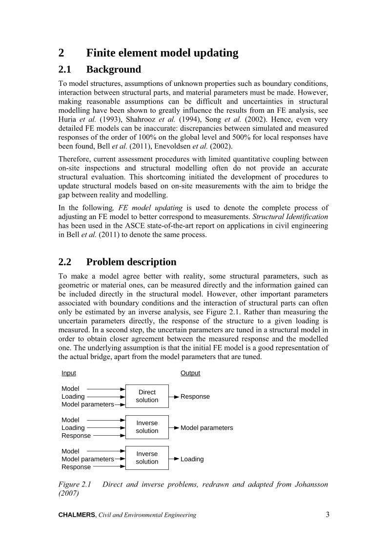
2.2 Problem description To make a model agree better with reality, some structural parameters, such as geometric or material ones, can be measured directly and the information gained can be included directly in the structural model. However, other important parameters associated with boundary conditions and the interaction of structural parts can often only be estimated by an inverse analysis, see Figure 2.1. Rather than measuring the uncertain parameters directly, the response of the structure to a given loading is measured. In a second step, the uncertain parameters are tuned in a structural model in order to obtain closer agreement between the measured response and the modelled one. The underlying assumption is that the initial FE model is a good representation of the actual bridge, apart from the model parameters that are tuned.
Input Output
ModelLoading ResponseModel parameters
ModelLoading Model parametersResponse
Model Model parameters LoadingResponse
Direct solution
Inverse solution
Inverse solution
Figure 2.1 Direct and inverse problems, redrawn and adapted from Johansson (2007)
4 CHALMERS, Civil and Environmental Engineering
However, as is typical for an inverse problem, estimating structural parameters by inverse analysis has often been shown to be an ill-posed problem. This means that it does not fulfil the requirements of a well-posed problem, namely existence, uniqueness and the stability of a solution, a definition which goes back to Hadamard (1902). In this context “stability” means that small variations of the initial model yield only small variations in the results. Researchers have noticed that many possible combinations of updating parameters in realistic ranges could be found, which have led to more accurate FE models, Zhang et al. (2001), Jaishi and Ren (2005); studies have shown that it is difficult to identify model parameters when a rather small amount of artificial noise is added to simulated measurements, Jaishi and Ren (2007), Bakir et al. (2008). It has been shown that measurements are often insensitive to structural changes, Brownjohn et al. (2001), Huth et al. (2005).
This makes it difficult to find updating parameters that are not just an arbitrary combination of model parameters, which conceal the measurement and remaining modelling errors, but are improved estimates of the actual structural parameters.
For bridge applications, two research initiatives tackled the problem of combining on-site measurements with structural modelling for bridge evaluation by using different approaches. The research approaches are here designated Bridge evaluation by static load testing and FE model updating in structural dynamics.
2.3 Bridge evaluation by static load testing When bridges are subjected to static loads, strains, forces and deformations are recorded, see Chajes et al. (1997), Barker (2001), Huang (2004). Depending on the purpose of the load test, a distinction between a proof load test and a diagnostic load test can be made, Cruz and Casas (2007), A. G. Lichtenstein and Associates (1998).
In proof load tests, the bridge is subjected to very high loads which include the risk of damage and collapse of the structure. The aim is to prove that the bridge has the required capacity. The information gained from the tests can be incorporated in the probabilistic model of the bridge to truncate the theoretical capacity distribution. Applications of proof load tests can be found in Nowak and Tharmabala (1988) and Moses et al. (1994).
The other branch of static load testing, i.e. diagnostic load testing, focuses on the structural model instead of the probabilistic model. A lower load level is often chosen and the load tests are used to improve the understanding of the bridge behaviour, as well as to verify and adjust the structural model. Uncertainties regarding material properties, boundary conditions, and interaction between structural parts can be reduced, and shortcomings of the structural model can be eliminated. The changes to the initial FE model are usually introduced manually; they are not limited to parametric changes to the model. Thus, all possible sources of modelling error can be reduced by justified changes.
A major problem of diagnostic load tests is the extrapolation of the measured bridge behaviour to other loads. Bridges can have non-stationary boundary conditions due to temperature and moisture changes, can show sudden releases of movement systems, and show nonlinear geometrical and material behaviour. Findings from the load test may therefore be invalid for other loading configurations. To take these things into account, it is required that the reason for the differences in structural behaviour
CHALMERS, Civil and Environmental Engineering 5
between the model and the real bridge be found. An overview of the effects in bridges that can lead to a significant different behaviour change from that initially assumed, and a discussion of whether they can be relied upon, can be found in Bakht and Jaeger (1990) and A. G. Lichtenstein and Associates (1998).
2.4 FE model updating in structural dynamics The term FE model updating in structural dynamics is used when an improved agreement between measured and computed modal (dynamic) data is desired. This branch emerged initially in mechanical and aerospace engineering and was later applied to civil engineering structures. When modal data are used to update a model, a distinction between direct and indirect updating methods can be made, Friswell and Mottershead (1995).
In direct methods, the mass, stiffness and damping matrixes are updated directly. The advantage of direct methods is that they do not require iterations, which eliminates the risk of divergence and excessive computational demands. However, the major drawback of direct methods is that the updated mass and stiffness matrix may lose their physical meaning.
In contrast to that, iterative methods solve the inverse problem, as the name implies, iteratively. Instead of directly changing the complete FE model, only uncertain model parameters are changed iteratively in order to make the FE model agree better with the measurements. The inverse problem is solved by a repeated solution of the direct problem as part of an iterative optimization procedure. When using optimisation algorithms to solve the inverse problem, the model changes introduced are usually restricted to parameter changes. Hence, only a part of the total modelling error can be reduced.
2.5 Proposed methodology The proposed and applied methodology for FE model updating aims to combine the advantages of the framework of diagnostic load tests with those of the mathematically more advanced concept of iterative methods for FE model updating in structural dynamics. This led to the methodology for FE model updating which is presented and applied in Paper I. It consists of three main steps.
1. The methodology starts from an FE model suited for the design of the bridge. First the lower bound assumptions, which are appropriate for the design of bridges but not for FE model updating, have to be removed. Second, manual model refinements are introduced to the FE model. This facilitates dealing with all kinds of modelling errors. This is followed by a sensitivity study to get an overview of model parameter sensitivities and to find improved estimates of model parameters.
2. Fine tuning of model parameters is done with the help of optimisation algorithms.
3. To make the updated model applicable for modelling untested conditions, it is necessary to evaluate the accuracy of the updated parameters and to find any possible sources of model parameter changes. Before using the model to analyse conditions that are different from the testing conditions, it may be
6 CHALMERS, Civil and Environmental Engineering
necessary to eliminate previously introduced model changes which do not hold for the conditions that are to be analysed.
2.6 Application to the new Svinesund Bridge
2.6.1 The new Svinesund Bridge
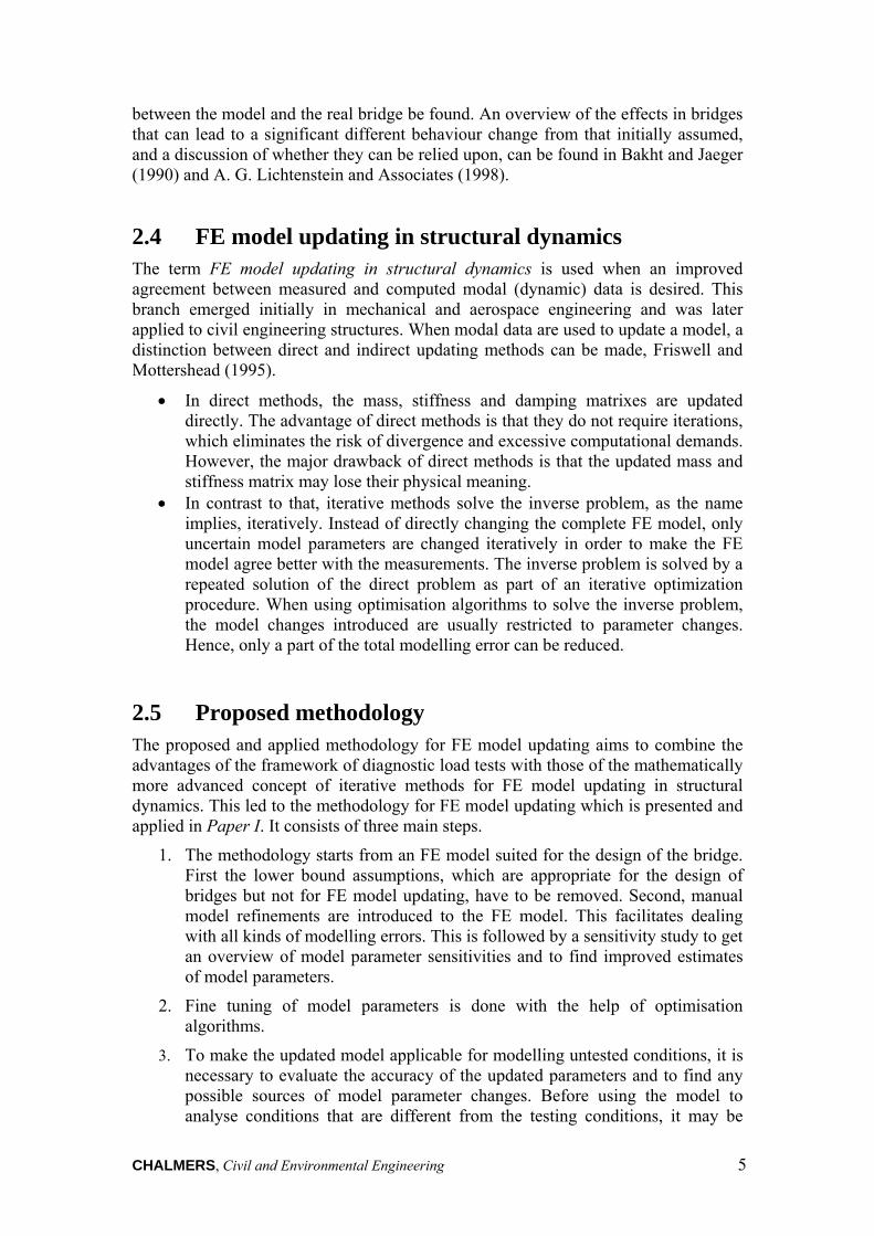
The new Svinesund Bridge was opened for traffic, in June 2005, as a part of the new European road E6 between Gothenburg and Oslo. The bridge connects Sweden and Norway over the Idefjord. With a total length of 704 m and a main span length of 247 m, it is one of the longest single arch bridges of the world, see Figure 2.2.
Figure 2.2 Elevation of the new Svinesund Bridge, from Darholm et al. (2007)
The two bridge deck girders carry two lanes of traffic each and are made of steel. In the side spans the bridge deck girders are supported, via cross beams, by concrete columns, while in the main span the cross beams are suspended from the concrete arch. The bridge deck girders are connected to the concrete arch where they pass the arch on either side. Due to the slender columns and the wide spacing of the bridge deck girders, it was necessary to prestress the bridge deck girders onto the columns to avoid uplifting during asymmetric loading.
When the new Svinesund Bridge was constructed, a measurement program was initiated to check and verify the response of the bridge. The programme started during the construction phase, included two days of testing before opening the bridge, and has been running during the first years of service of the bridge, see James and Karoumi (2003), Ülker-Kaustell and Karoumi (2006) and Karoumi and Andersson (2007).
Due to the available measurements, the new Svinesund Bridge was chosen for a case study for FE model updating. The data used to update the FE model included in total 264 measurements of four types. This large amount of data reduced the risk of non-unique solutions of the updating procedure, which can occur when a small number of measurements is used to update a large number of model parameters.
2.6.2 Updating of the finite element model
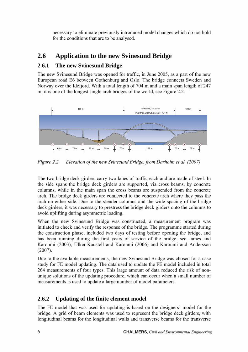
The FE model that was used for updating is based on the designers’ model for the bridge. A grid of beam elements was used to represent the bridge deck girders, with longitudinal beams for the longitudinal walls and transverse beams for the transverse
CHALMERS, Civil and Environmental Engineering 7
walls, see Figure 2.3. The columns and the arch were also represented by beam elements. Shear deformations were included by using Timoshenko beam theory. Including the temporary supporting structures, the FE model had 11 724 degrees of freedom. A more detailed description of the FE model, including details of the model conversion into the FE software package ABAQUS, can be found in Plos and Movaffaghi (2004).
Figure 2.3 FE model of the new Svinesund Bridge
The manual model refinements included:
Increasing the Young’s modulus of the arch to account for the reinforcement in the arch and the further hardening up to the day of load testing,
Remodelling of the bearing behaviour of the bridge, Including the non-structural mass, and Increasing the bridge deck stiffness.
For fine tuning of model parameters, the Nelder-Mead simplex algorithm, Nelder and Mead (1965), was used to avoid convergence problems of gradient-based optimisation algorithms. Parameters that were fine tuned were:
The elastic modulus of the arch, The elastic modulus of the bridge deck, The static friction threshold of the bearings, and The mass of non-structural elements along the bridge deck girder.
2.6.3 Results of updating
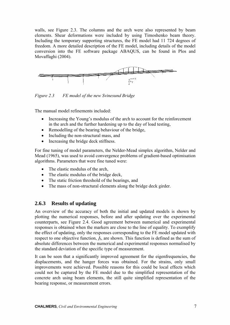
An overview of the accuracy of both the initial and updated models is shown by plotting the numerical responses, before and after updating over the experimental counterparts, see Figure 2.4. Good agreement between numerical and experimental responses is obtained when the markers are close to the line of equality. To exemplify the effect of updating, only the responses corresponding to the FE model updated with respect to one objective function, J3, are shown. This function is defined as the sum of absolute differences between the numerical and experimental responses normalised by the standard deviation of the specific type of measurement.
It can be seen that a significantly improved agreement for the eigenfrequencies, the displacements, and the hanger forces was obtained. For the strains, only small improvements were achieved. Possible reasons for this could be local effects which could not be captured by the FE model due to the simplified representation of the concrete arch using beam elements, the still quite simplified representation of the bearing response, or measurement errors.
8 CHALMERS, Civil and Environmental Engineering
The updated model parameters remained within reasonable ranges; the reason could be found for the changes that were manually introduced into the model before the parameter study.
(a) (b)
(c) (d)
Figure 2.4 A comparison of the accuracy of initial and updated model: (a) Eigenfrequencies, (b) Strains, (c) Displacements, (d) Hanger forces.
2.7 General recommendations To obtain improved agreement between measured and modelled response, model parameters are often fine tuned. However, in the study of the new Svinesund Bridge, including the nonlinear bearing behaviour, was shown to offer a major improvement of the model accuracy. This showed the importance of the nonlinear response of the
CHALMERS, Civil and Environmental Engineering 9
structure and modelling assumptions that go beyond uncertain model parameters. Therefore, only changing model parameters by using optimisation algorithms seldom leads to model parameters which are improved estimates of the real structural parameters. Instead the model parameters will be calibrated to conceal inappropriate modelling assumptions.
The combination of static and modal measurements showed that different bearing behaviours during ambient vibrations and under the load test must be assumed. Hence, to update the bearing parameters using modal data and to use these parameters for the evaluation of the bridge under static loading can be impossible.
Despite the large number of measurements, it was not possible to update the rotational stiffness of the arch support. The parameter study showed that the target responses were insensitive to this parameter, which made it impossible to update it parameter by inverse analysis. This shows that a careful choice of measurement program is needed. Prior to determining the programme, a sensitivity study is therefore recommended. By changing uncertain model parameters in the a priori FE model, the sensitivity of measurable responses to model parameters changes can be studied. This can be used to find an appropriate measurement program which allows estimating all uncertain model parameters.
The use of the Nelder-Mead simplex algorithm for fine tuning of the model parameters is recommended to avoid the convergence problems of gradient based optimisation algorithms.

10 CHALMERS, Civil and Environmental Engineering
CHALMERS, Civil and Environmental Engineering 11
3 Safety Evaluation of Concrete Structures with Nonlinear Analysis
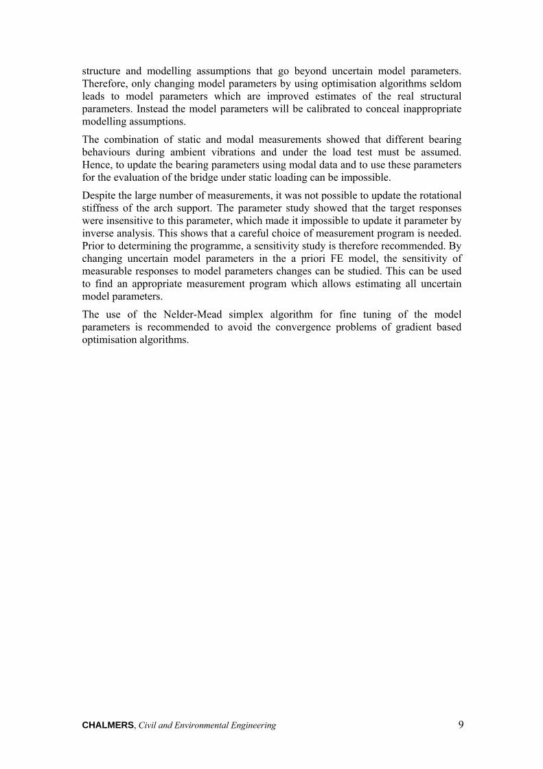
3.1 Background The verification of a structure or a structural component can be done on three different levels: the structural level, the sectional level or the material level, see Figure 3.1. Depending on the chosen level, the verification is done using an inequality of forces, generalised stresses, or stresses.
Figure 3.1 Possible levels for verification
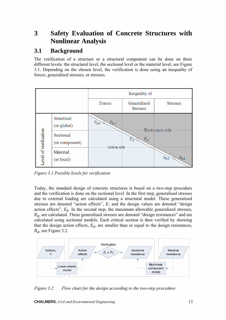
Today, the standard design of concrete structures is based on a two-step procedure and the verification is done on the sectional level. In the first step, generalised stresses due to external loading are calculated using a structural model. These generalised stresses are denoted “action effects”, , and the design values are denoted “design action effects”, . In the second step, the maximum allowable generalised stresses,
, are calculated. These generalised stresses are denoted “design resistances” and are calculated using sectional models. Each critical section is then verified by showing that the design action effects, , are smaller than or equal to the design resistances,
, see Figure 3.2.
Figure 3.2 Flow chart for the design according to the two-step procedure
12 CHALMERS, Civil and Environmental Engineering
This standard two-step procedure is inconsistent because incompatible constitutive relations are assumed in both the structural model and the sectional resistance models. The structural model is usually based on the assumption of a linear-elastic material response, while the sectional resistance models account for the nonlinear material behaviour. Linear-elastic structural models do not allow the structural response to be modelled realistically. Cracking, which occurs even under service loads, yielding of the reinforcement and crushing of concrete for higher loads, cannot be captured. In addition, the release of restraining forces and the deformation increase due to cracking also cannot be modelled. Nor is it possible to utilise the full capacity of structures by redistribution. For advanced structures it can also be difficult to identify critical sections; only highly simplified resistance models are available.
To overcome the drawbacks of the two-step procedure, nonlinear analysis is increasingly used to calculate the failure load directly as part of a one-step procedure. ‘Nonlinear analysis’ is used here to denote an analysis which accounts for the nonlinear stress-strain relationship of the concrete and reinforcement steel, and allows for redistribution; it can be used to calculate the failure load of a structure directly. The load is usually increased incrementally and the constitutive models employed automatically guarantee equilibrium in all parts of the structures. This means that the nonlinear analysis fulfils the purpose of both the structural model and the sectional models according to the two-step procedure, see Figure 3.3. Additional manual sectional checks are needed only for failure modes that cannot be described by the nonlinear analysis.
The distinction between action effects and sectional resistances is well suited for the two-step procedure as two separate models are used. However, for the one-step procedure, when a single nonlinear analysis is used, it is more common to distinguish between external and internal forces. External forces are acting on the nonlinear model and it checks if internal forces can be found to balance the external forces. Therefore, the verification for the one-step procedure is usually done on the structural level by an inequality of forces.
For the ultimate load, which corresponds to the final load step at which the nonlinear analysis finds equilibrium, there are many expressions, such as “theoretical ultimate load” and “structural load bearing capacity” by König et al. (1995), “theoretical carrying capacity of the system” by König et al. (1997), the load at which “there is global failure of the structure“ in EN 1992-2, and “(global) resistance” by Model Code 2010 fib (2010a) fib (2010b), Cervenka et al. (2007), Henriques et al. (2002) and Six (2001). In this thesis “ultimate structural resistance” will be used. The following symbols have been used in the past:
by König et al. (1995), by König et al. (1997), in EN 1992-2, and by Model Code 2010, fib (2010a) fib (2010b), Cervenka et al. (2007),
Henriques et al. (2002) and Six (2001).
Here, the symbol R is used (“ ” was used in Paper II, III and IV). The design value here is called “design structural resistance” with the symbol, R .
CHALMERS, Civil and Environmental Engineering 13
To denote the forces obtained from the Eurocodes which are applied on the nonlinear model, i.e. the design actions, different symbols have been used:
· · by König et al. (1995) and in EN 1992-2, in the Model Code 2010 and by Six (2001), and by Henriques et al. (2002).
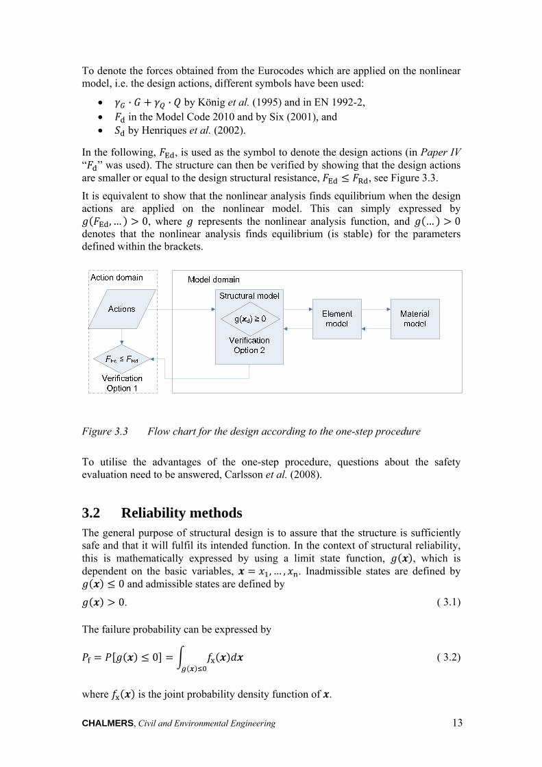
In the following, E , is used as the symbol to denote the design actions (in Paper IV “ ” was used). The structure can then be verified by showing that the design actions are smaller or equal to the design structural resistance, E R , see Figure 3.3.
It is equivalent to show that the nonlinear analysis finds equilibrium when the design actions are applied on the nonlinear model. This can simply expressed by
E , … 0, where represents the nonlinear analysis function, and … 0 denotes that the nonlinear analysis finds equilibrium (is stable) for the parameters defined within the brackets.
Figure 3.3 Flow chart for the design according to the one-step procedure
To utilise the advantages of the one-step procedure, questions about the safety evaluation need to be answered, Carlsson et al. (2008).
3.2 Reliability methods The general purpose of structural design is to assure that the structure is sufficiently safe and that it will fulfil its intended function. In the context of structural reliability, this is mathematically expressed by using a limit state function, , which is dependent on the basic variables, , … , . Inadmissible states are defined by
0 and admissible states are defined by
0. ( 3.1)
The failure probability can be expressed by
0 ( 3.2)
where is the joint probability density function of .
14 CHALMERS, Civil and Environmental Engineering
Even though the performance of the structure itself is of primary interest, the limit state function is often formulated on the component level. To evaluate reliability the different methods available are commonly subdivided into three levels.
3.2.1 Level III methods
Level III methods are fully probabilistic ones which use the failure probability as a reliability measure. Provided that an accurate stochastic model is available, Level III methods allow failure probabilities to be computed accurately. The most common Level III methods are Numerical Integration and Monte Carlo simulations, but there are also more efficient modifications, Waarts (2000).
Numerical integration is used to approximate the integral from Equation 3.2 numerically. The joint probability function is evaluated for a finite set of integration points to construct an interpolation function. Polynomials which are easy to integrate are usually chosen for the interpolation function. By transforming the random variables from the X-space into the U-space, i.e. the standard normal space, the integral according to Equation 3.2 can be solved by multiple summation as
… U ∆ ( 3.3)
where U is the joint probability function and is the indicator function defined by
0 if 01 if 0
. ( 3.4)
The efficiency of numerical integration decreases exponentially with an increase of random variables. This makes numerical integration inefficient for problems which involve many random variables.
Monte Carlo simulations rely on repeated random experiments to approximate the failure probability by the relative number of experiments for which
0. The failure probability is approximated to
1 ( 3.5)
where N is the number of experiments and is the sample, , from . Monte Carlo simulations are widely applicable and easy to implement. However, for small failure probabilities, a high number of random experiments is needed to obtain accurate estimates of the failure probability. This makes Monte Carlo simulations computationally expensive in these cases. To increase the efficiency of Monte Carlo simulations, a safe area can be excluded from sampling. In Paper III previous limit state function evaluations were used to establish bounds to classify a safe set of the sample space. If the
CHALMERS, Civil and Environmental Engineering 15
bounds allowed placing a new sample in the safe set, no limit state function evaluation was necessary. By this a reduction of computation time was gained.
3.2.2 Level II methods
Level II methods use approximations of the limit state function to calculate the reliability index, , as a reliability measure, instead of the failure probability. Haldar and Mahadevan (2000) further subdivide Level II methods.
Mean value first-order second-moment methods which are based on a first-order Taylor series expansion of the limit state function at the mean values of the random variables. Random variables are only represented by the first two moments, i.e. mean and covariance. Examples are the Cornell reliability index and the Rosenbleuth-Esteva reliability index, see Cornell (1969) and Rosenbleuth and Esteva (1972).
Advanced first-order method for normal variables was used by Haldar and Mahadevan (2000) to denote the Hasofer-Lind method, Hasofer and Lind (1974). To compute the Hasofer-Lind reliability index requires that the limit state function be rewritten in terms of reduced variables, i.e. with random variables of zero mean and unit standard deviation. The reliability index is then defined as the shortest distance from the origin of the coordinate system to the limit state surface. The point on the limit state surface that minimises the distance is called “design point”. The design point is usually not known a priori but can be found by an iterative procedure.
Advanced first-order methods for non-normal variables can be seen as an extension of the Hasofer-Lind method to non-normal random variables. This can be achieved by a transformation of the non-normal random variables into standardized equivalent normal variables, e.g. by the normal trail, Rosenblatt, or Nataf transformation. Detailed information about these algorithms is available, Ditlevsen and Madsen (2007) and Melchers (1999). Due to the use of more than second moment information, advanced first-order methods for non-normal variables have also been classified as Level III methods, Madsen et al. (1986).
Second-Order Reliability Methods (SORM) use a second order approximation of the failure function around the design point. This yields more accurate results for failure functions, which are heavily nonlinear around the design point.
For most structural applications Level II methods can be considered to be sufficiently accurate, CEN (2002a).
3.2.3 Level I methods
Instead of evaluating the failure probability by Level III methods or calculating the reliability index according to Level II methods, Level I can only be used to verify that a sufficient reliability level is obtained. Uncertain parameters are modelled by a single or a few representative values, e.g. upper and lower characteristic values, , , which correspond to predetermined fractile values. Partial factors, , are used to calculate
16 CHALMERS, Civil and Environmental Engineering
the design values, , , from the characteristic values to , , , or
, , ⁄ . It is then assumed that a sufficient reliability level is obtained if
0. ( 3.6)
For favourable parameters, e.g. material strengths, the characteristic value must be decreased to obtain the design value. For unfavourable parameters, e.g. loads, the characteristic values must be increased. Often it is possible to predetermine wheather parameters are favourable or unfavourable a priori. However, generally it is required to check Equation 3.6 for all possible combinations of increased and decreased design values. This requires 2 checks, where is the number of random variables.
The partial factor method used in the Eurocodes, CEN (2002a), is a Level I method. To derive the design values according to Eurocodes, fixed sensitivity factors, E0.7 and R 0.8, for the action/action effect and resistance were assumed, CEN (2002a). The design resistance, , and design action effects, , can then be defined independent with Φ R and Φ E , where Φ is the cumulative distribution function, and is the target reliability, i.e. 3.8 for a reference period of 50 years for reliability class RC2 according to CEN (2002a). Equation 3.6 can be expressed by
, 0. ( 3.7)
Frequently, when designing according to the two-step procedure, a separation between action effect and resistance calculation can be assumed. In this case Equation 3.7 can be simplified to
. ( 3.8)
Detailed rules about the calculation of design action effects and design resistances of concrete structures are available, CEN (2002a), CEN (2002b), CEN (2004).
3.2.4 Limitation of reliability methods
For the building industry only extremely small failure probabilities are usually acceptable, which requires that the random variables can be described accurately in the extreme tails of the distributions. This information is not usually available in practical applications. Furthermore, structural failures are often a result of more or less gross human errors, Andersson et al. (2010), which are difficult to describe by random variables. Therefore, calculated failure probabilities must be viewed as operational values, for code calibration purposes or the relative comparison of structures, i.e. not as good approximations of actual failure rates, CEN (2002a). Consequently, current codes such as the Eurocodes are based primarily on existing design practices, CEN (2002a); however calibration to superior reliability methods has also been performed.
CHALMERS, Civil and Environmental Engineering 17
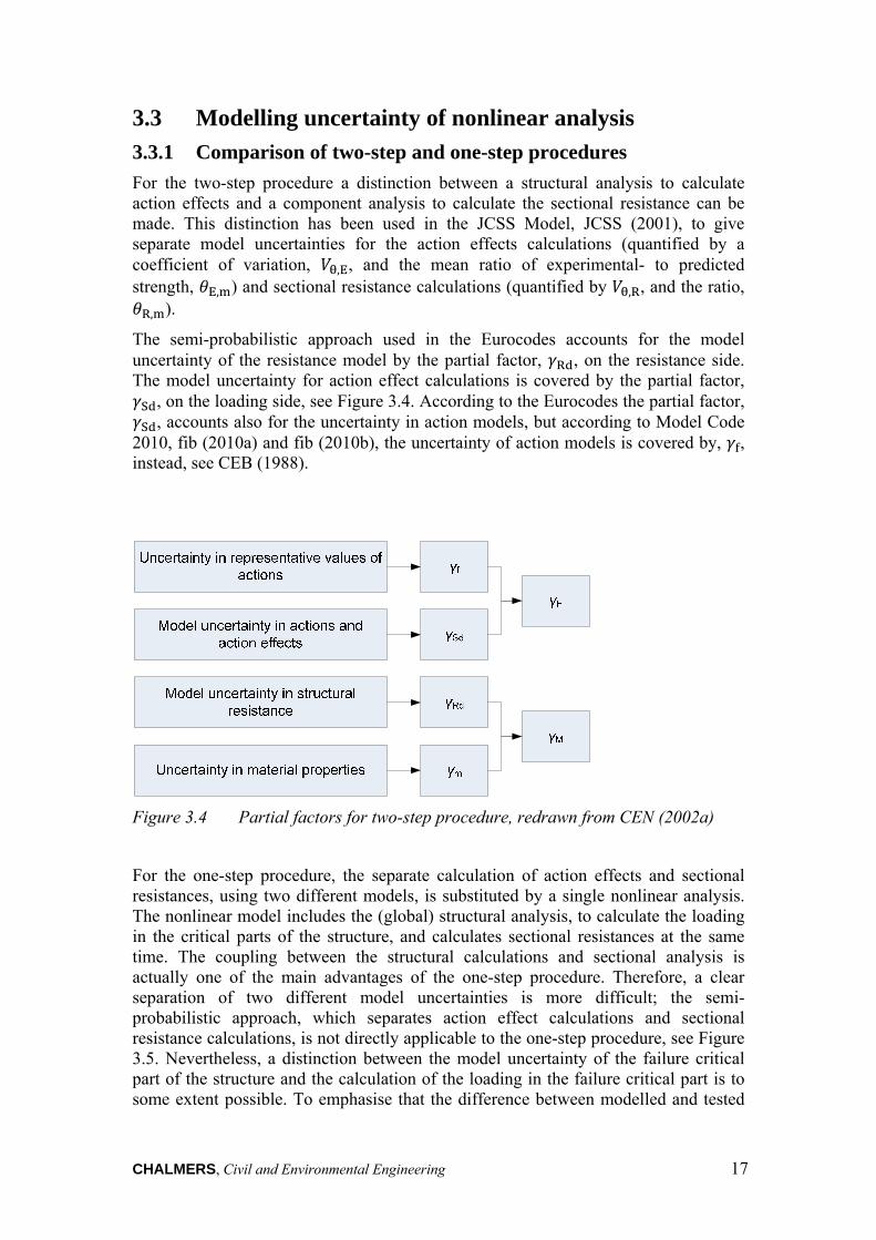
3.3 Modelling uncertainty of nonlinear analysis
3.3.1 Comparison of two-step and one-step procedures
For the two-step procedure a distinction between a structural analysis to calculate action effects and a component analysis to calculate the sectional resistance can be made. This distinction has been used in the JCSS Model, JCSS (2001), to give separate model uncertainties for the action effects calculations (quantified by a coefficient of variation, ,E, and the mean ratio of experimental- to predicted strength, E, ) and sectional resistance calculations (quantified by ,R, and the ratio,
R, ).
The semi-probabilistic approach used in the Eurocodes accounts for the model uncertainty of the resistance model by the partial factor, R , on the resistance side. The model uncertainty for action effect calculations is covered by the partial factor,
S , on the loading side, see Figure 3.4. According to the Eurocodes the partial factor, S , accounts also for the uncertainty in action models, but according to Model Code
2010, fib (2010a) and fib (2010b), the uncertainty of action models is covered by, , instead, see CEB (1988).
Figure 3.4 Partial factors for two-step procedure, redrawn from CEN (2002a)
For the one-step procedure, the separate calculation of action effects and sectional resistances, using two different models, is substituted by a single nonlinear analysis. The nonlinear model includes the (global) structural analysis, to calculate the loading in the critical parts of the structure, and calculates sectional resistances at the same time. The coupling between the structural calculations and sectional analysis is actually one of the main advantages of the one-step procedure. Therefore, a clear separation of two different model uncertainties is more difficult; the semi-probabilistic approach, which separates action effect calculations and sectional resistance calculations, is not directly applicable to the one-step procedure, see Figure 3.5. Nevertheless, a distinction between the model uncertainty of the failure critical part of the structure and the calculation of the loading in the failure critical part is to some extent possible. To emphasise that the difference between modelled and tested
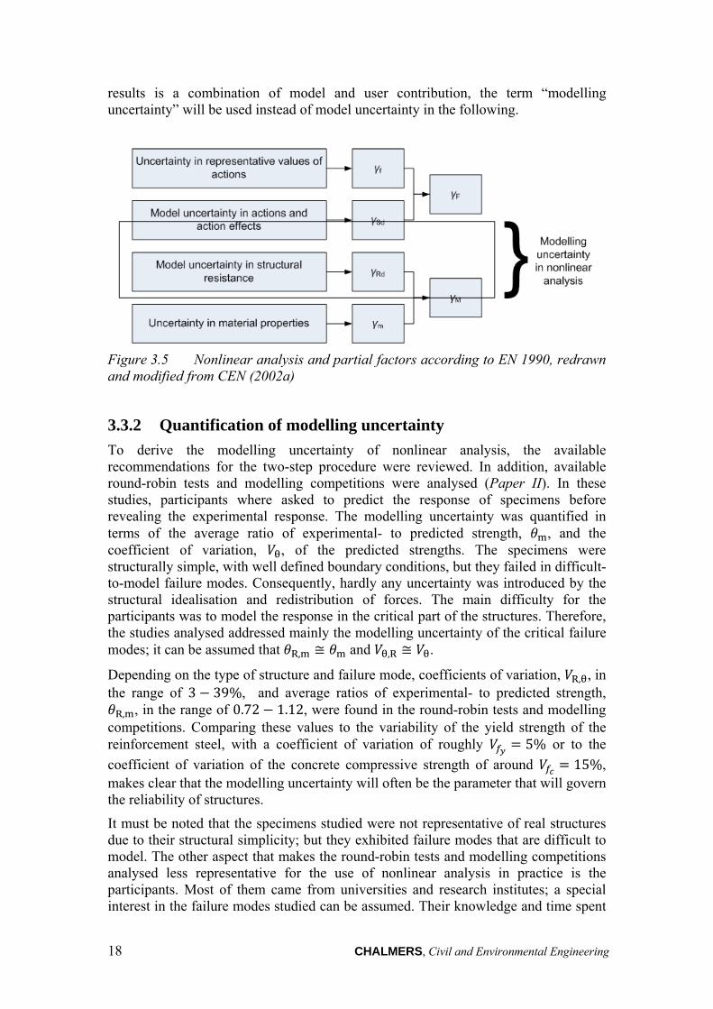
18 CHALMERS, Civil and Environmental Engineering
results is a combination of model and user contribution, the term “modelling uncertainty” will be used instead of model uncertainty in the following.
Figure 3.5 Nonlinear analysis and partial factors according to EN 1990, redrawn and modified from CEN (2002a)
3.3.2 Quantification of modelling uncertainty
To derive the modelling uncertainty of nonlinear analysis, the available recommendations for the two-step procedure were reviewed. In addition, available round-robin tests and modelling competitions were analysed (Paper II). In these studies, participants where asked to predict the response of specimens before revealing the experimental response. The modelling uncertainty was quantified in terms of the average ratio of experimental- to predicted strength, , and the coefficient of variation, , of the predicted strengths. The specimens were structurally simple, with well defined boundary conditions, but they failed in difficult-to-model failure modes. Consequently, hardly any uncertainty was introduced by the structural idealisation and redistribution of forces. The main difficulty for the participants was to model the response in the critical part of the structures. Therefore, the studies analysed addressed mainly the modelling uncertainty of the critical failure modes; it can be assumed that R, and ,R .
Depending on the type of structure and failure mode, coefficients of variation, R, , in the range of 3 39%, and average ratios of experimental- to predicted strength,
R, , in the range of 0.72 1.12, were found in the round-robin tests and modelling competitions. Comparing these values to the variability of the yield strength of the reinforcement steel, with a coefficient of variation of roughly 5% or to the
coefficient of variation of the concrete compressive strength of around 15%, makes clear that the modelling uncertainty will often be the parameter that will govern the reliability of structures.
It must be noted that the specimens studied were not representative of real structures due to their structural simplicity; but they exhibited failure modes that are difficult to model. The other aspect that makes the round-robin tests and modelling competitions analysed less representative for the use of nonlinear analysis in practice is the participants. Most of them came from universities and research institutes; a special interest in the failure modes studied can be assumed. Their knowledge and time spent
CHALMERS, Civil and Environmental Engineering 19
on the task is most likely different from that of engineers working in practice. Therefore, the modelling uncertainties observed can only be seen as a rough approximation of the modelling uncertainty of nonlinear analysis used in practice.
3.4 Available safety formats for nonlinear analysis Early safety formats for nonlinear analysis of concrete structures were only applicable when moment-curvature relations , as constitutive laws were used. However, with the emergence of nonlinear analysis based on stress-strain relations , new approaches were developed. In the following quite recent proposals are summarised. An overview of earlier developments related to CEB can be found in Mancini (2002) and Henriques et al. (2002). The safety formats included here focus on the resistance side. The actions or action effects must be treated according to CEN (2002a) and CEN (2002b).
3.4.1 The partial factor method
The partial factor method is primarily used to calculate design sectional resistances of beams and columns that are loaded by bending moments and normal forces when using EN 1992-1-1 and EN 1992-2, CEN (2004), CEN (2005). However, the Model Code 2010, fib (2010a) and fib (2010b), proposes the use design material parameters for nonlinear analysis.
Partial factors, C and S, are used to calculate design material strengths, and , from the characteristic material strengths, and , according to
C ( 3.9)
S . ( 3.10)
The partial factors, C and S, can be derived based on the assumption that the relation between the resistance, , and nominal resistance, , can be expressed in multiplicative form. This means that the resistance, , can be expressed as a product of, a factor to account for the resistance modelling uncertainty, R, a geometrical variable, , and a material strength variable, , and the nominal resistance, :
R · . ( 3.11)
This allows the coefficient of variation of the resistance to be approximated:
R ,R ( 3.12)
where ,R, and are the coefficients of variation of the associated parameters. According to the European Concrete Platform (2008), the coefficients of variation according to Table 3.1 can be assumed to be the basis for the partial factors according to CEN (2004).
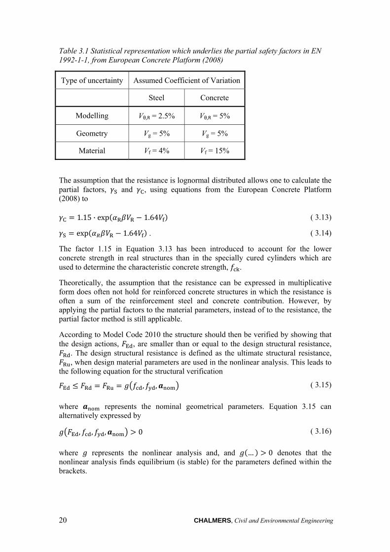
20 CHALMERS, Civil and Environmental Engineering
Table 3.1 Statistical representation which underlies the partial safety factors in EN 1992-1-1, from European Concrete Platform (2008)
Type of uncertainty Assumed Coefficient of Variation
Steel Concrete
Modelling Vθ,R = 2.5% Vθ,R = 5%
Geometry Vg = 5% Vg = 5%
Material Vf = 4% Vf = 15%
The assumption that the resistance is lognormal distributed allows one to calculate the partial factors, S and C, using equations from the European Concrete Platform (2008) to
The factor 1.15 in Equation 3.13 has been introduced to account for the lower concrete strength in real structures than in the specially cured cylinders which are used to determine the characteristic concrete strength, .
Theoretically, the assumption that the resistance can be expressed in multiplicative form does often not hold for reinforced concrete structures in which the resistance is often a sum of the reinforcement steel and concrete contribution. However, by applying the partial factors to the material parameters, instead of to the resistance, the partial factor method is still applicable.
According to Model Code 2010 the structure should then be verified by showing that the design actions, E , are smaller than or equal to the design structural resistance,
R . The design structural resistance is defined as the ultimate structural resistance, R , when design material parameters are used in the nonlinear analysis. This leads to
the following equation for the structural verification
where represents the nominal geometrical parameters. Equation 3.15 can alternatively expressed by
where represents the nonlinear analysis and, and … 0 denotes that the nonlinear analysis finds equilibrium (is stable) for the parameters defined within the brackets.
C 1.15 · exp R R 1.64 ( 3.13)
S exp R 1.64 . ( 3.14)
E R R , , ( 3.15)
E , , , 0 ( 3.16)
CHALMERS, Civil and Environmental Engineering 21
3.4.2 The global resistance factor method
Accounting for all resistance uncertainty by a reduction of material parameters results in very low material values. Such low material parameters lead to an overestimation of deformations and underestimation of restraint forces, which means they cannot be used to realistically model the response of concrete structures. Therefore, a modification to the partial factor method was proposed by König et al. (1997) and included in the Model Code 2010. König et al. (1997) proposed to use more realistic material strengths, and calculated as
According to Model Code 2010 the structure should then be verified by:
or when using the previously introduced notation:
where R 1.06 is the partial factor to account for the resistance model uncertainty, and R 1.2 is the partial factor for the resistance. Inserting the recommended values into Equation 3.20 and expressing everything in terms of design material parameters yields
This makes clear that using increased design material parameters requires for actions which must be increased beyond the design values from CEN (2002b) in the nonlinear analysis, i.e. the use of more realistic material parameters comes at the cost of using less realistic actions. In addition, Equations 3.20 and 3.21 make clear that the notation “resistance safety factors” for, R, can be misleading as the resistance safety factors are actually used to increase the actions beyond the design values, E .
3.4.3 The safety format according to EN 1992-2
The safety format for nonlinear analysis according to EN 1992-2 CEN (2005) is based on the global resistance factor method, and the same material parameters, and , are used in nonlinear analysis. However, objections to verification on the structural level by an inequality of forces have led to a reformulation of the safety format on the sectional level using an inequality of generalised stresses, Mancini (2002) and Bertagnoli et al. (2004). Depending on the load level, the generalised stresses from the nonlinear analysis are either denoted action effect, , or resistance, , CEN (2005). The EN 1992-2 provides three alternative equations which can be used to assure an intended reliability level:
1.1 S C⁄ ( 3.17)
1.1 ( 3.18)
E RR , ,
R R ( 3.19)
R R E , , , 0 ( 3.20)
1.27 E , 1.27 , 1.27 , 0. ( 3.21)
22 CHALMERS, Civil and Environmental Engineering
where G and Q are the partial factors for the action effects which include the model uncertainty, and are the partial factors for the action effects without the action effect model uncertainty, S 1.15 is the partial factor for the model uncertainty of action effects, and represent the permanent and variable actions.
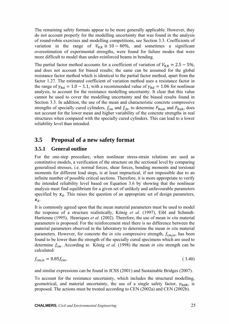
The use of generalised stresses in critical sections to verify an intended reliability level is impractical and can be impossible. Common nonlinear analysis toolboxes do not support the comparison of generalised stresses for different load steps which requires that the verification is done manually. In addition, for more advanced analysis based on nonlinear stress-strain relations, as shown in Figure 3.6, it can be impossible to limit the number of critical sections for which verifications are needed. This leads theoretically to an infinite number of possible sections which must be verified. For most structures in which action effects increase monotonically for increasing loading, Equation 3.23 and Equation 3.19 give the same results.
Figure 3.6. Crack pattern for a box girder bridge, from Broo (2008)
3.4.4 The estimated coefficient of variation method
Due to difficulties in verifying the structures on the sectional level when using the safety format according to EN 1992-2, Cervenka et al. (2007) revived the idea of verification of the structure by an inequality of forces. To be able to realistically model the structural response, the use of mean material strengths, and , in the nonlinear analysis was proposed. The mean material parameters are used to calculate the ultimate structural resistance, R , at which the structure fails:
To quantify the sensitivity of the ultimate structural resistance to material changes, the use of a second nonlinear analysis using characteristic material parameters, and
R G QR
R ( 3.22)
G QR
R R R
O ( 3.23)
R SR
R. ( 3.24)
R , , . ( 3.25)
CHALMERS, Civil and Environmental Engineering 23
, has been proposed to calculate the “characteristic” ultimate structural resistance,
R :
The mean and characteristic ultimate resistances are used to estimate the coefficient of variation of the resistance, :
This is used to calculate a resistance safety factor, R:
In the initial proposal by Cervenka et al. (2007) there was no guidance on how to account for the modelling uncertainty and geometrical uncertainty. However, when the proposal was included in Model Code 2010, fib (2010a) and fib (2010b), the use of the model uncertainty factor, R 1.06, was recommended to verify the structure:
3.4.5 The safety format according to Six (2001)
Six (2001) employs the probabilistic analysis of slender columns to establish an equation to calculate a resistance safety factor, R, for these types of structural elements. The material parameters for the nonlinear analysis are calculated:
where is a coefficient taking into account long term effects. The safety factor depends on numerous parameters of the section that causes failure according to two equations and a linear interpolation in between:
where is the strain of the tensile reinforcement (or the less compressed reinforcement layer), C 1 1.1 /500⁄ 1 is an extra safety factor for high strength concrete ( in MPa), is the total reinforcement ratio, / is the ratio of the reinforcement amount of the most compressed layer to the least compressed layer, and 1% is a normalisation reinforcement ratio. Besides these safety factors, Six (2001) introduced an additional safety factor, , to account for the
R , , . ( 3.26)
.ln R
R. ( 3.27)
R exp R . ( 3.28)
E RR , ,
R R ( 3.29)
R R E , , , 0. ( 3.30)
1.1 ( 3.31)
1.1 ( 3.32)
R, 1.3 for 0.004 ( 3.33)
R, 1.1 C C
.for 0 ( 3.34)
24 CHALMERS, Civil and Environmental Engineering
system reliability and the model uncertainty of the structural model. However, no information about how this factor can be quantified is given. The structure should then be verified:
3.4.6 The safety format according to Henriques et al. (2002)
Henriques et al. (2002) used the probabilistic analysis of beam sections and beams with clamped ends subjected to bending moments to derive a safety format. According to their proposal the mean concrete strength, , and the mean steel yield strength, , should be used in the nonlinear analysis. They proposed to define the safety factor, R R, “as a function of a parameter measuring the ductility of the structural response” and mentioned the facture energy as a possible parameter. For frame structures they used the relative position of the neutral axis, / , of the section where the failure occurs as a measure to quantify the resistance safety factor, R R, where is the compressive zone depth and is the effective depth of the cross section. The resistance safety factor should then be calculated:
where is a constant that takes into account the influence of the redistribution of forces between critical sections and should be calculated according to the concrete compressive class: 0.9 for C20 and 0.8 for C40, with linear interpolation in between. This leads to two equations for the structural verification:
3.4.7 Discussion of existing safety formats
The safety formats according to Six (2001) and Henriques et al. (2002) have been formulated for special types of structural elements, namely columns subjected to an eccentric normal force and beams subjected to bending. Therefore, they are not applicable to other types of structures.
The safety format according to EN 1992-2, CEN (2005), which relies on an inequality of generalised stresses, i.e. stress integrants over a section, is not suitable for nonlinear analysis based on nonlinear material laws. For this type of analysis it can be difficult to limit the number of critical sections that need to be verified.
E RR . , . ,
R ( 3.35)
R E , 1.1 , 1.1 , 0. ( 3.36)
R R
; 0.35
; 0.35 ( 3.37)
E RR , ,
R R ( 3.38)
R R E , , , 0. ( 3.39)
CHALMERS, Civil and Environmental Engineering 25
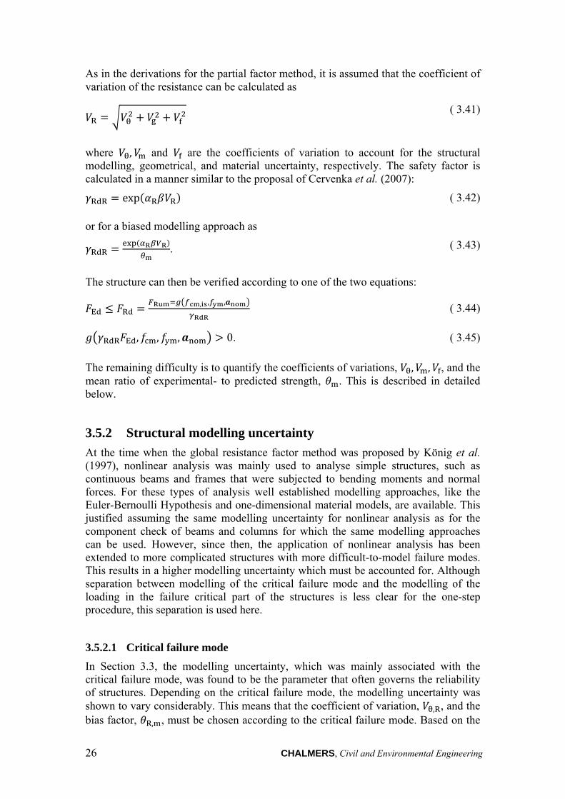
The remaining safety formats appear to be more generally applicable. However, they do not account properly for the modelling uncertainty that was found in the analysis of round-robin exercises and modelling competitions, see Section 3.3. Coefficients of variation in the range of ,R 10 40%, and sometimes a significant overestimation of experimental strengths, were found for failure modes that were more difficult to model than under-reinforced beams in bending.
The partial factor method accounts for a coefficient of variation of ,R 2.5 5%, and does not account for biased results; the same can be assumed for the global resistance factor method which is identical to the partial factor method, apart from the factor 1.27. The estimated coefficient of variation method uses a resistance factor in the range of R 1.0 1.1, with a recommended value of R 1.06 for nonlinear analysis, to account for the resistance modelling uncertainty. It clear that this value cannot be used to cover the modelling uncertainty and the biased results found in Section 3.3. In addition, the use of the mean and characteristic concrete compressive strengths of specially cured cylinders, and , to determine R and R , does not account for the lower mean and higher variability of the concrete strengths in real structures when compared with the specially cured cylinders. This can lead to a lower reliability level than intended.
3.5 Proposal of a new safety format
3.5.1 General outline
For the one-step procedure, when nonlinear stress-strain relations are used as constitutive models, a verification of the structure on the sectional level by comparing generalised stresses, i.e. normal forces, shear forces, bending moments and torsional moments for different load steps, is at least impractical, if not impossible due to an infinite number of possible critical sections. Therefore, it is more appropriate to verify the intended reliability level based on Equation 3.6 by showing that the nonlinear analysis must find equilibrium for a given set of unlikely and unfavourable parameters specified by . This raises the question of an appropriate set of design parameters,
.
It is commonly agreed upon that the mean material parameters must be used to model the response of a structure realistically, König et al. (1997), Eibl and Schmidt-Hurtienne (1995), Henriques et al. (2002). Therefore, the use of mean in situ material parameters is proposed. For the reinforcement steel there is no difference between the material parameters observed in the laboratory to determine the mean in situ material parameters. However, for concrete the in situ compressive strength, , , has been found to be lower than the strength of the specially cured specimens which are used to determine . According to König et al. (1998) the mean in situ strength can be calculated:
and similar expressions can be found in JCSS (2001) and Sustainable Bridges (2007).
To account for the resistance uncertainty, which includes the structural modelling, geometrical, and material uncertainty, the use of a single safety factor, R R, is proposed. The actions must be treated according to CEN (2002a) and CEN (2002b).
, 0.85 , ( 3.40)
26 CHALMERS, Civil and Environmental Engineering
As in the derivations for the partial factor method, it is assumed that the coefficient of variation of the resistance can be calculated as
R ( 3.41)
where , and are the coefficients of variation to account for the structural modelling, geometrical, and material uncertainty, respectively. The safety factor is calculated in a manner similar to the proposal of Cervenka et al. (2007):
R R exp R R ( 3.42)
or for a biased modelling approach as
R RR R . ( 3.43)
The structure can then be verified according to one of the two equations:
The remaining difficulty is to quantify the coefficients of variations, , , , and the mean ratio of experimental- to predicted strength, . This is described in detailed below.
3.5.2 Structural modelling uncertainty
At the time when the global resistance factor method was proposed by König et al. (1997), nonlinear analysis was mainly used to analyse simple structures, such as continuous beams and frames that were subjected to bending moments and normal forces. For these types of analysis well established modelling approaches, like the Euler-Bernoulli Hypothesis and one-dimensional material models, are available. This justified assuming the same modelling uncertainty for nonlinear analysis as for the component check of beams and columns for which the same modelling approaches can be used. However, since then, the application of nonlinear analysis has been extended to more complicated structures with more difficult-to-model failure modes. This results in a higher modelling uncertainty which must be accounted for. Although separation between modelling of the critical failure mode and the modelling of the loading in the failure critical part of the structures is less clear for the one-step procedure, this separation is used here.
3.5.2.1 Critical failure mode
In Section 3.3, the modelling uncertainty, which was mainly associated with the critical failure mode, was found to be the parameter that often governs the reliability of structures. Depending on the critical failure mode, the modelling uncertainty was shown to vary considerably. This means that the coefficient of variation, ,R, and the bias factor, R, , must be chosen according to the critical failure mode. Based on the
E RR , , ,
R R ( 3.44)
R R E , , , 0. ( 3.45)
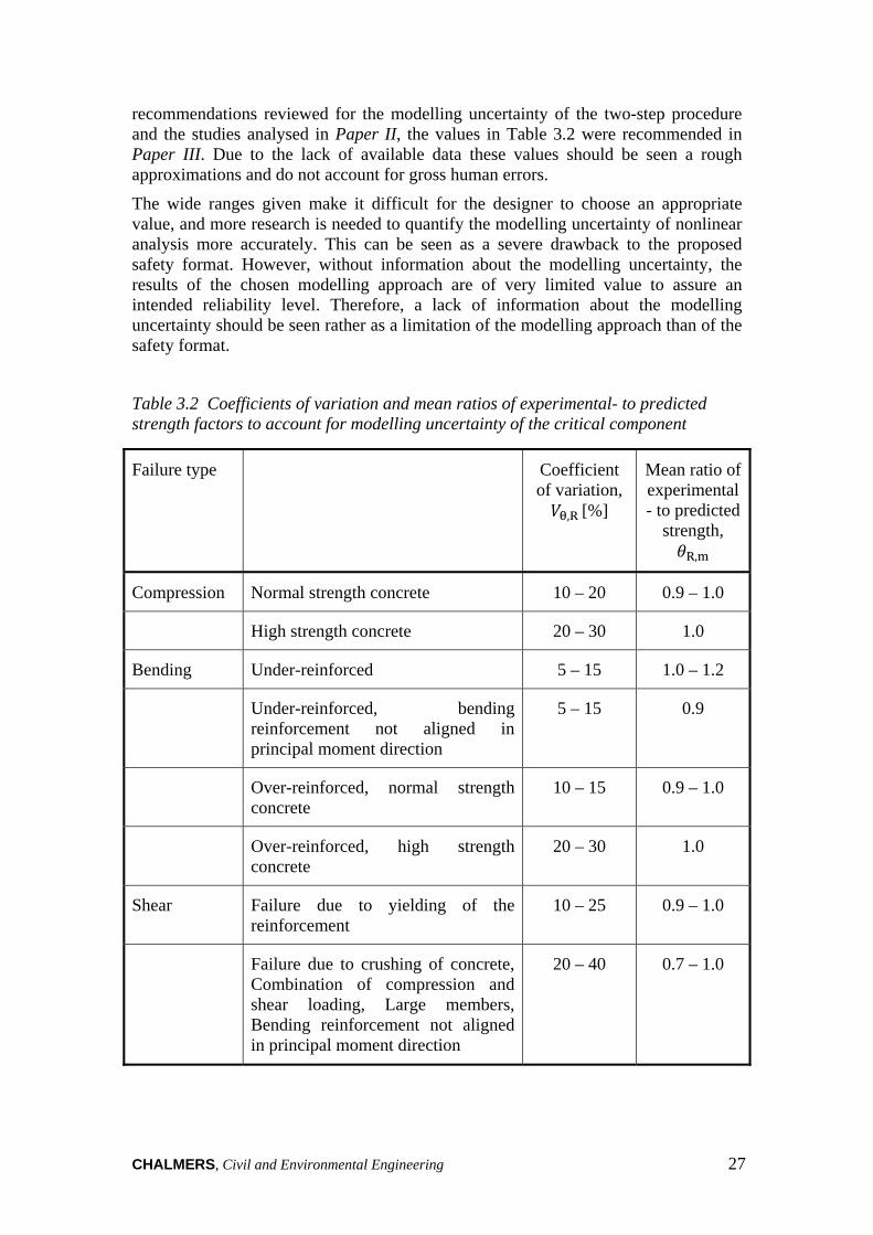
CHALMERS, Civil and Environmental Engineering 27
recommendations reviewed for the modelling uncertainty of the two-step procedure and the studies analysed in Paper II, the values in Table 3.2 were recommended in Paper III. Due to the lack of available data these values should be seen a rough approximations and do not account for gross human errors.
The wide ranges given make it difficult for the designer to choose an appropriate value, and more research is needed to quantify the modelling uncertainty of nonlinear analysis more accurately. This can be seen as a severe drawback to the proposed safety format. However, without information about the modelling uncertainty, the results of the chosen modelling approach are of very limited value to assure an intended reliability level. Therefore, a lack of information about the modelling uncertainty should be seen rather as a limitation of the modelling approach than of the safety format.
Table 3.2 Coefficients of variation and mean ratios of experimental- to predicted strength factors to account for modelling uncertainty of the critical component
Failure type Coefficient of variation,
,R [%]
Mean ratio of experimental- to predicted
strength, R,
Compression Normal strength concrete 10 – 20 0.9 – 1.0
High strength concrete 20 – 30 1.0
Bending Under-reinforced 5 – 15 1.0 – 1.2
Under-reinforced, bending reinforcement not aligned in principal moment direction
5 – 15 0.9
Over-reinforced, normal strength concrete
10 – 15 0.9 – 1.0
Over-reinforced, high strength concrete
20 – 30 1.0
Shear Failure due to yielding of the reinforcement
10 – 25 0.9 – 1.0
Failure due to crushing of concrete, Combination of compression and shear loading, Large members, Bending reinforcement not aligned in principal moment direction
20 – 40 0.7 – 1.0
28 CHALMERS, Civil and Environmental Engineering
3.5.2.2 Loading in the failure critical part of a structure
For statically indeterminate structures, the uncertainty of the loading in the failure critical part of the structure must be taken into account. However, the modelling competitions and round-robin tests analysed did not allow quantifying this uncertainty. The uncertainty of loading in the failure critical part of the structure is similar to the uncertainty of action effect calculations for the two-step procedure. This has been quantified with coefficients of variation in JCSS (2001) which recommends values in the range of 5 20%, see Table 3.3.
Table 3.3 Recommended probabilistic models for model uncertainties of action effect calculations, from JCSS (2001)
Coefficient of variation,
,E[%]
Mean value,
E,
Moments in frames 10 1
Axial forces in frames 5 1
Shear forces in frames 10 1
Moments in plates 20 1
Forces in plates 10 1
3.5.2.3 Two options
There are two options to account for the modelling uncertainty for the one-step procedure. The first option is more in line with the semi-probabilistic approach. The modelling uncertainty of the loading in the failure critical part of the structures is accounted for on the action side by the factor, S , which is included in the partial factor, F, see Figure 3.7. In this case the coefficient of variation to account for the modelling uncertainty can be calculated to ,R and the mean ratio of experimental- to predicted strength to R, .
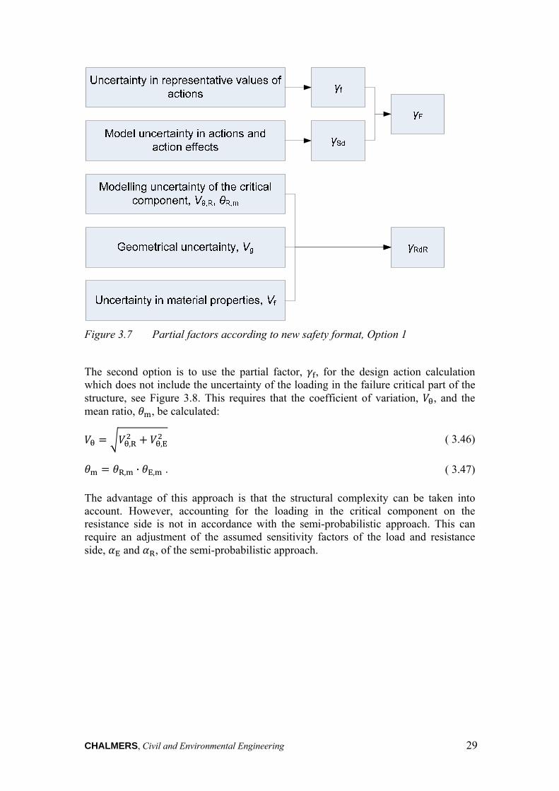
CHALMERS, Civil and Environmental Engineering 29
Figure 3.7 Partial factors according to new safety format, Option 1
The second option is to use the partial factor, , for the design action calculation which does not include the uncertainty of the loading in the failure critical part of the structure, see Figure 3.8. This requires that the coefficient of variation, , and the mean ratio, , be calculated:
The advantage of this approach is that the structural complexity can be taken into account. However, accounting for the loading in the critical component on the resistance side is not in accordance with the semi-probabilistic approach. This can require an adjustment of the assumed sensitivity factors of the load and resistance side, E and R, of the semi-probabilistic approach.
,R ,E ( 3.46)
R, · E, . ( 3.47)
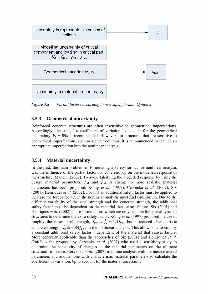
30 CHALMERS, Civil and Environmental Engineering
Figure 3.8 Partial factors according to new safety format, Option 2
3.5.3 Geometrical uncertainty
Reinforced concrete structures are often insensitive to geometrical imperfections. Accordingly, the use of a coefficient of variation to account for the geometrical uncertainty, 5% is recommended. However, for structures that are sensitive to geometrical imperfections, such as slender columns, it is recommended to include an appropriate imperfection into the nonlinear analysis.
3.5.4 Material uncertainty
In the past, the main problem in formulating a safety format for nonlinear analysis was the influence of the partial factor for concrete, C, on the modelled response of the structure, Mancini (2002). To avoid falsifying the modelled response by using the design material parameters, and , a change to more realistic material parameters has been proposed, König et al. (1997), Cervenka et al. (2007), Six (2001), Henriques et al. (2002). For this an additional safety factor must be applied to increase the forces for which the nonlinear analysis must find equilibrium. Due to the different variability of the steel strength and the concrete strength, the additional safety factor must be dependent on the material that causes failure. Six (2001) and Henriques et al. (2002) chose formulations which are only suitable for special types of structures to determine the extra safety factor. König et al. (1997) proposed the use of roughly the mean steel strength, 1.1 , but a reduced characteristic
concrete strength, 0.84 , in the nonlinear analysis. This allows one to employ a constant additional safety factor independent of the material that causes failure. More generally applicable than the approaches of Six (2001) and Henriques et al. (2002) is the proposal by Cervenka et al. (2007) who used a sensitivity study to determine the sensitivity of changes in the material parameters on the ultimate structural resistance. Cervenka et al. (2007) used one analysis with the mean material parameters and another one with characteristic material parameters to calculate the coefficient of variation, , to account for the material uncertainty.
CHALMERS, Civil and Environmental Engineering 31
In this thesis work, instead of decreasing both material strengths at the same time, it was decided to test reducing one material strength at a time. Generally, this required three additional nonlinear analyses to calculate the ultimate structural resistances:
with decreased concrete compressive strength
R ,∆ , exp c V,
, , , , ,
with decrease concrete tensile strength to calculate
R ,∆ , , , exp cV,
, , and
with decreased steel strength,
R ,∆ , , , , exp cV ,
where R ,∆ , R ,∆ and R ,∆ are the ultimate structural resistances when
decreased concrete compressive strength, decreased concrete tensile strength and decreased steel strength were used as input parameters; c is the step size parameter; V
,, V
, and V are the coefficients of variation of the in situ concrete compressive
strength, in situ concrete tensile strength and yield strength of the reinforcement, respectively; and , is the mean in situ concrete tensile strength.
In similarity to the Gauss-approximation formula, but with an increased step size, the coefficient of variation to account for the material strength uncertainty can then be calculated as
where ∆ , ∆ and ∆ are the step sizes by which the material strengths were decreased;
,,
, and are the variance of the in situ concrete compressive
strength, in situ concrete tensile strength and the yield strength of the reinforcement steel, respectively.
In Paper II this approach was compared with the proposal by Cervenka et al. (2007) on beams in bending for which only the concrete compressive strength and the strength of the reinforcement steel could cause failure. Five step size parameters, c, to decrease the material parameters were tested. It was found that the most accurate results were obtained when Equation 3.48 was used with a step size parameter of c 2.15.
Paper III examined further a less conservative approach to quantify the material uncertainty and to calculate the coefficient of variation:
However, only minor differences were found between Equations 3.48 and 3.49.
3.6 Testing of the new safety format At first a test was conducted to determine whether the safety format leads to the target reliability of the resistance side according to the semi-probabilistic approach of
R
R R ,∆
∆ ,
R R ,∆
∆ ,
R R ,∆
∆
( 3.48)
Rmax R R ,∆
∆ ,, R R ,∆
∆ ,,
R R ,∆
∆. ( 3.49)
32 CHALMERS, Civil and Environmental Engineering
R 3.04. For comparison the same test was made for the safety format according to EN 1992-2. Then the loads were also included in the evaluation of the safety format, to see whether the new safety format, in combination with the provisions of EN 1990, CEN (2002a), yields the target reliability of 3.8. In a third step, the new safety format and three safety formats presented in the Model Code 2010 were applied to a concrete frame bridge for which the design structural resistances were compared.
3.6.1 Resistance side
To test whether the safety format leads to the target reliability of the resistance side, according to the semi-probabilistic approach of R 3.04, it was used to calculate the design structural resistance according to
The same was done for the safety format according to EN 1992-2. Then full probabilistic analysis was used to calculate the probability that the resistance is below the design resistance, , and the corresponding reliability index, R
Φ , where Φ is the standard normal distribution function. Testing of the new safety format is presented for:
Beam sections in bending in Paper II, Short columns subjected to a normal force in Schlune et al. (2011) Beam sections subjected to shear forces in Schlune et al. (2011), and Beam sections subject to a combination of bending moment and shear force in
Paper III.
The mean reliability indexes for the design according to EN 1992-2, EN, and for the new safety format, , and the corresponding coefficients of variation,
EN, and
, , are summarised in Table 3.4.
It can be seen that the design according to EN 1992-2 led to a good agreement for beams in bending when a small modelling uncertainty of ,R 5% was assumed. However, when a higher modelling uncertainty was assumed, EN 1992-2 led to reliability indexes that were below the target reliability.
The new safety format led to a much closer agreement with the target reliability regardless of the component analysed. The higher the assumed modelling uncertainty was the closer the agreement was to the target reliability.
It must be noted that the comparison between the safety formats is not entirely fair. To calculate the safety factor, R R, for the new safety format, the same coefficient of variation, ,R, and ratio, R, , as in the full probabilistic analyses were assumed. The same holds for the mean material strengths and variability of the material strengths. In practical applications of the new safety format only approximations of these values can be used, which results in a higher variability of the reliability indexes obtained.
, , ,
R R. ( 3.50)
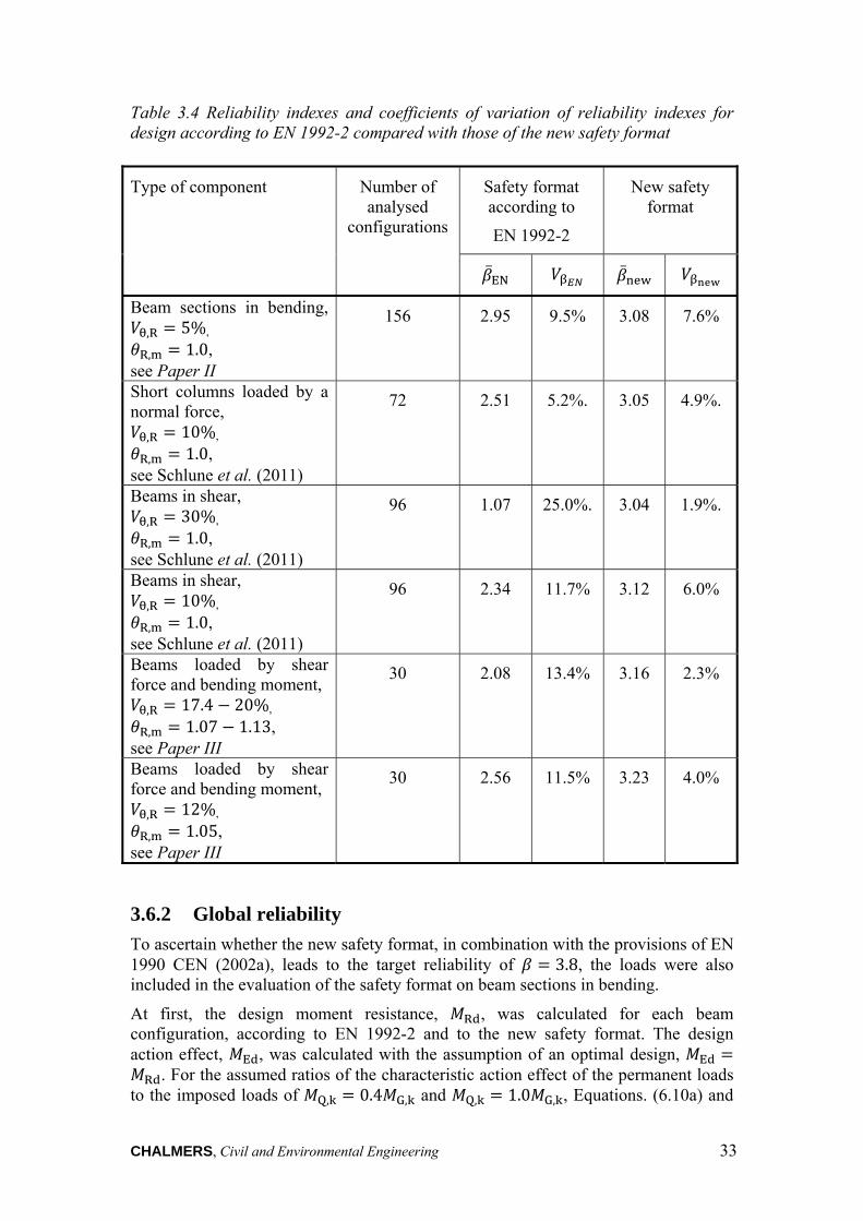
CHALMERS, Civil and Environmental Engineering 33
Table 3.4 Reliability indexes and coefficients of variation of reliability indexes for design according to EN 1992-2 compared with those of the new safety format
3.6.2 Global reliability
To ascertain whether the new safety format, in combination with the provisions of EN 1990 CEN (2002a), leads to the target reliability of 3.8, the loads were also included in the evaluation of the safety format on beam sections in bending.
At first, the design moment resistance, R , was calculated for each beam configuration, according to EN 1992-2 and to the new safety format. The design action effect, E , was calculated with the assumption of an optimal design, E
R . For the assumed ratios of the characteristic action effect of the permanent loads to the imposed loads of Q, 0.4 G, and Q, 1.0 G, , Equations. (6.10a) and
Type of component Number of analysed
configurations
Safety format according to
EN 1992-2
New safety format
EN
Beam sections in bending, ,R 5%,
R, 1.0, see Paper II
156 2.95 9.5% 3.08 7.6%
Short columns loaded by a normal force,
,R 10%,
R, 1.0, see Schlune et al. (2011)
72 2.51 5.2%. 3.05 4.9%.
Beams in shear, ,R 30%,
R, 1.0, see Schlune et al. (2011)
96 1.07 25.0%. 3.04 1.9%.
Beams in shear, ,R 10%,
R, 1.0, see Schlune et al. (2011)
96 2.34 11.7% 3.12 6.0%
Beams loaded by shear force and bending moment,
,R 17.4 20%,
R, 1.07 1.13, see Paper III
30 2.08 13.4% 3.16 2.3%
Beams loaded by shear force and bending moment,
,R 12%,
R, 1.05, see Paper III
30 2.56 11.5% 3.23 4.0%
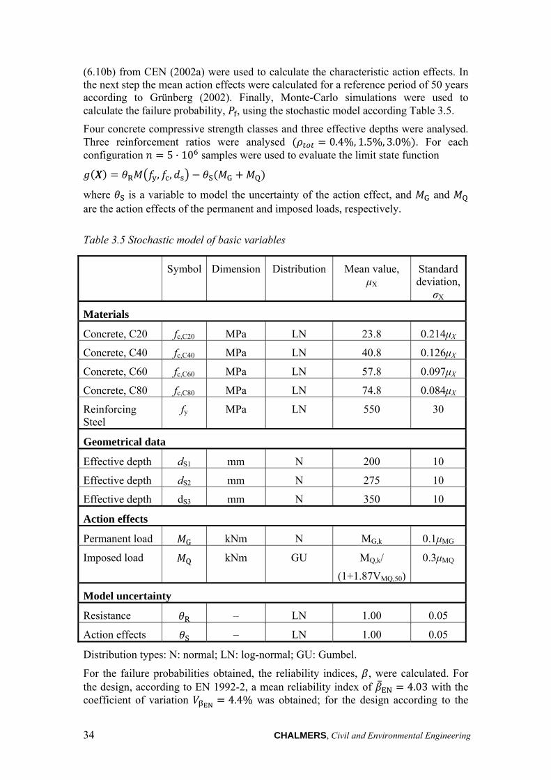
34 CHALMERS, Civil and Environmental Engineering
(6.10b) from CEN (2002a) were used to calculate the characteristic action effects. In the next step the mean action effects were calculated for a reference period of 50 years according to Grünberg (2002). Finally, Monte-Carlo simulations were used to calculate the failure probability, , using the stochastic model according Table 3.5.
Four concrete compressive strength classes and three effective depths were analysed. Three reinforcement ratios were analysed 0.4%, 1.5%, 3.0% . For each configuration 5 · 10 samples were used to evaluate the limit state function
R , , S G Q
where S is a variable to model the uncertainty of the action effect, and G and Q are the action effects of the permanent and imposed loads, respectively.
Table 3.5 Stochastic model of basic variables
Symbol Dimension Distribution Mean value, μX
Standard deviation,
σX
Materials
Concrete, C20 fc,C20 MPa LN 23.8 0.214μX
Concrete, C40 fc,C40 MPa LN 40.8 0.126μX
Concrete, C60 fc,C60 MPa LN 57.8 0.097μX
Concrete, C80 fc,C80 MPa LN 74.8 0.084μX
Reinforcing Steel
fy MPa LN 550 30
Geometrical data
Effective depth dS1 mm N 200 10
Effective depth dS2 mm N 275 10
Effective depth dS3 mm N 350 10
Action effects
Permanent load G kNm N MG,k 0.1μMG
Imposed load Q kNm GU MQ,k/
(1+1.87VMQ,50)
0.3μMQ
Model uncertainty
Resistance R – LN 1.00 0.05
Action effects S – LN 1.00 0.05
Distribution types: N: normal; LN: log-normal; GU: Gumbel.
For the failure probabilities obtained, the reliability indices, , were calculated. For the design, according to EN 1992-2, a mean reliability index of EN 4.03 with the coefficient of variation
EN4.4% was obtained; for the design according to the
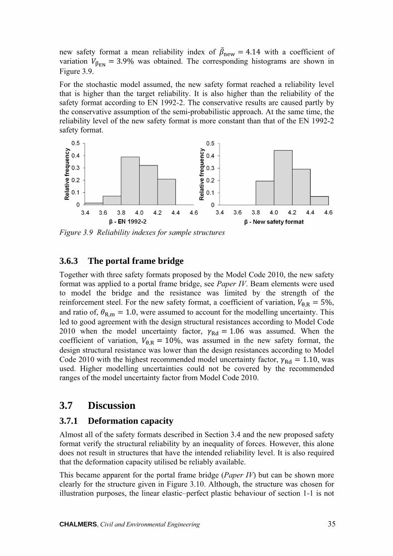
CHALMERS, Civil and Environmental Engineering 35
new safety format a mean reliability index of 4.14 with a coefficient of variation
EN3.9% was obtained. The corresponding histograms are shown in
Figure 3.9.
For the stochastic model assumed, the new safety format reached a reliability level that is higher than the target reliability. It is also higher than the reliability of the safety format according to EN 1992-2. The conservative results are caused partly by the conservative assumption of the semi-probabilistic approach. At the same time, the reliability level of the new safety format is more constant than that of the EN 1992-2 safety format.
Figure 3.9 Reliability indexes for sample structures
3.6.3 The portal frame bridge
Together with three safety formats proposed by the Model Code 2010, the new safety format was applied to a portal frame bridge, see Paper IV. Beam elements were used to model the bridge and the resistance was limited by the strength of the reinforcement steel. For the new safety format, a coefficient of variation, ,R 5%, and ratio of, R, 1.0, were assumed to account for the modelling uncertainty. This led to good agreement with the design structural resistances according to Model Code 2010 when the model uncertainty factor, R 1.06 was assumed. When the coefficient of variation, ,R 10%, was assumed in the new safety format, the design structural resistance was lower than the design resistances according to Model Code 2010 with the highest recommended model uncertainty factor, R 1.10, was used. Higher modelling uncertainties could not be covered by the recommended ranges of the model uncertainty factor from Model Code 2010.
3.7 Discussion
3.7.1 Deformation capacity
Almost all of the safety formats described in Section 3.4 and the new proposed safety format verify the structural reliability by an inequality of forces. However, this alone does not result in structures that have the intended reliability level. It is also required that the deformation capacity utilised be reliably available.
This became apparent for the portal frame bridge (Paper IV) but can be shown more clearly for the structure given in Figure 3.10. Although, the structure was chosen for illustration purposes, the linear elastic–perfect plastic behaviour of section 1-1 is not
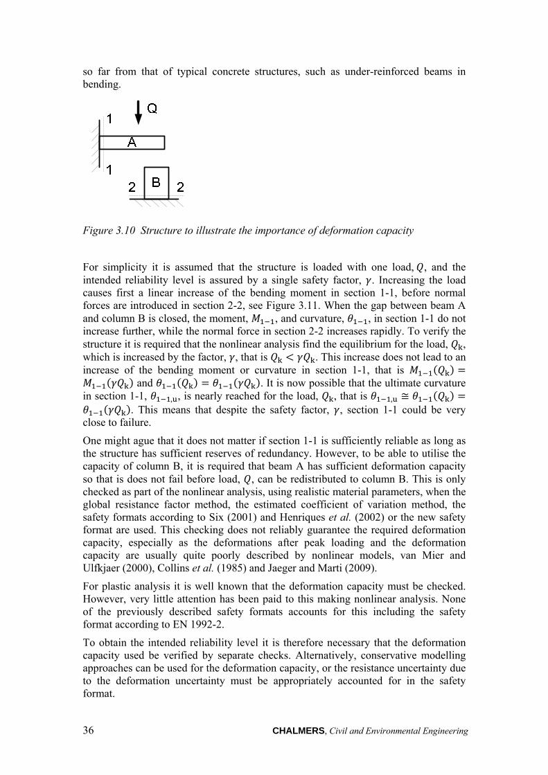
36 CHALMERS, Civil and Environmental Engineering
so far from that of typical concrete structures, such as under-reinforced beams in bending.
Figure 3.10 Structure to illustrate the importance of deformation capacity
For simplicity it is assumed that the structure is loaded with one load, , and the intended reliability level is assured by a single safety factor, . Increasing the load causes first a linear increase of the bending moment in section 1-1, before normal forces are introduced in section 2-2, see Figure 3.11. When the gap between beam A and column B is closed, the moment, , and curvature, , in section 1-1 do not increase further, while the normal force in section 2-2 increases rapidly. To verify the structure it is required that the nonlinear analysis find the equilibrium for the load, , which is increased by the factor, , that is . This increase does not lead to an increase of the bending moment or curvature in section 1-1, that is
and . It is now possible that the ultimate curvature in section 1-1, , , is nearly reached for the load, , that is ,
. This means that despite the safety factor, , section 1-1 could be very close to failure.
One might ague that it does not matter if section 1-1 is sufficiently reliable as long as the structure has sufficient reserves of redundancy. However, to be able to utilise the capacity of column B, it is required that beam A has sufficient deformation capacity so that is does not fail before load, , can be redistributed to column B. This is only checked as part of the nonlinear analysis, using realistic material parameters, when the global resistance factor method, the estimated coefficient of variation method, the safety formats according to Six (2001) and Henriques et al. (2002) or the new safety format are used. This checking does not reliably guarantee the required deformation capacity, especially as the deformations after peak loading and the deformation capacity are usually quite poorly described by nonlinear models, van Mier and Ulfkjaer (2000), Collins et al. (1985) and Jaeger and Marti (2009).
For plastic analysis it is well known that the deformation capacity must be checked. However, very little attention has been paid to this making nonlinear analysis. None of the previously described safety formats accounts for this including the safety format according to EN 1992-2.
To obtain the intended reliability level it is therefore necessary that the deformation capacity used be verified by separate checks. Alternatively, conservative modelling approaches can be used for the deformation capacity, or the resistance uncertainty due to the deformation uncertainty must be appropriately accounted for in the safety format.
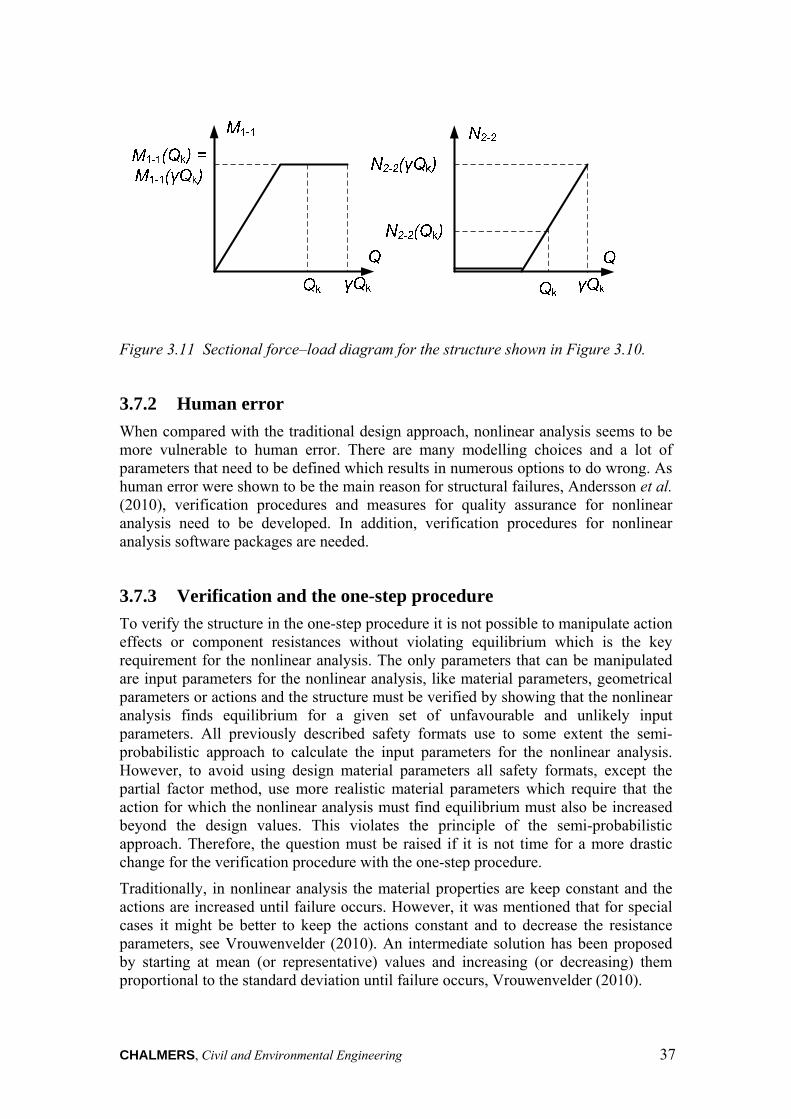
CHALMERS, Civil and Environmental Engineering 37
Figure 3.11 Sectional force–load diagram for the structure shown in Figure 3.10.
3.7.2 Human error
When compared with the traditional design approach, nonlinear analysis seems to be more vulnerable to human error. There are many modelling choices and a lot of parameters that need to be defined which results in numerous options to do wrong. As human error were shown to be the main reason for structural failures, Andersson et al. (2010), verification procedures and measures for quality assurance for nonlinear analysis need to be developed. In addition, verification procedures for nonlinear analysis software packages are needed.
3.7.3 Verification and the one-step procedure
To verify the structure in the one-step procedure it is not possible to manipulate action effects or component resistances without violating equilibrium which is the key requirement for the nonlinear analysis. The only parameters that can be manipulated are input parameters for the nonlinear analysis, like material parameters, geometrical parameters or actions and the structure must be verified by showing that the nonlinear analysis finds equilibrium for a given set of unfavourable and unlikely input parameters. All previously described safety formats use to some extent the semi-probabilistic approach to calculate the input parameters for the nonlinear analysis. However, to avoid using design material parameters all safety formats, except the partial factor method, use more realistic material parameters which require that the action for which the nonlinear analysis must find equilibrium must also be increased beyond the design values. This violates the principle of the semi-probabilistic approach. Therefore, the question must be raised if it is not time for a more drastic change for the verification procedure with the one-step procedure.
Traditionally, in nonlinear analysis the material properties are keep constant and the actions are increased until failure occurs. However, it was mentioned that for special cases it might be better to keep the actions constant and to decrease the resistance parameters, see Vrouwenvelder (2010). An intermediate solution has been proposed by starting at mean (or representative) values and increasing (or decreasing) them proportional to the standard deviation until failure occurs, Vrouwenvelder (2010).

38 CHALMERS, Civil and Environmental Engineering
Another similar solution can be to start again at mean (or representative) values. In the next step a sensitivity analysis is used to determine the importance of model parameters. This can e.g. be done by decreasing each favourable parameter within a reasonable range or until failure is reached. The same must be done for all unfavourable parameter which must be increased. In a final nonlinear analysis the parameters can then be increased or decreased proportional to their sensitivity until failure is reached. This can then be used to calculate an approximate reliability index,
.
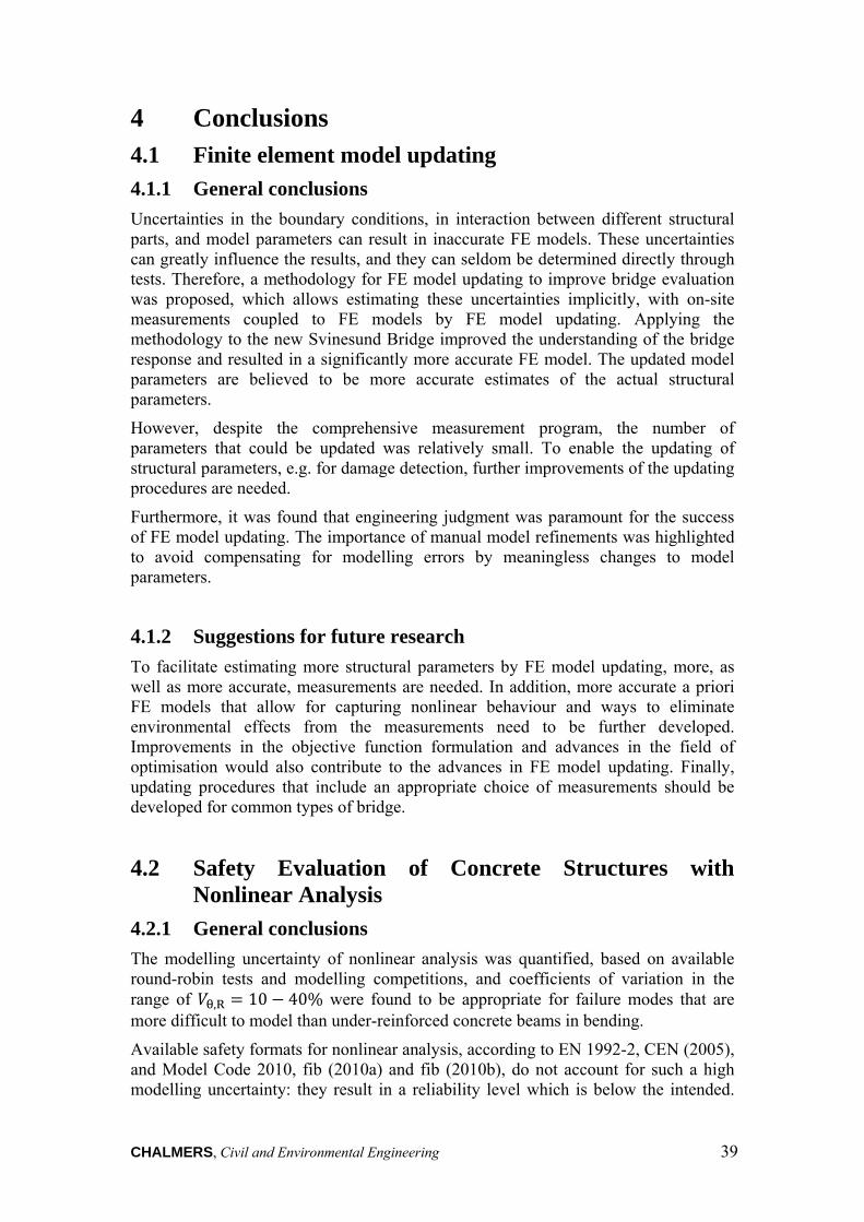
CHALMERS, Civil and Environmental Engineering 39
4 Conclusions 4.1 Finite element model updating
4.1.1 General conclusions
Uncertainties in the boundary conditions, in interaction between different structural parts, and model parameters can result in inaccurate FE models. These uncertainties can greatly influence the results, and they can seldom be determined directly through tests. Therefore, a methodology for FE model updating to improve bridge evaluation was proposed, which allows estimating these uncertainties implicitly, with on-site measurements coupled to FE models by FE model updating. Applying the methodology to the new Svinesund Bridge improved the understanding of the bridge response and resulted in a significantly more accurate FE model. The updated model parameters are believed to be more accurate estimates of the actual structural parameters.
However, despite the comprehensive measurement program, the number of parameters that could be updated was relatively small. To enable the updating of structural parameters, e.g. for damage detection, further improvements of the updating procedures are needed.
Furthermore, it was found that engineering judgment was paramount for the success of FE model updating. The importance of manual model refinements was highlighted to avoid compensating for modelling errors by meaningless changes to model parameters.
4.1.2 Suggestions for future research
To facilitate estimating more structural parameters by FE model updating, more, as well as more accurate, measurements are needed. In addition, more accurate a priori FE models that allow for capturing nonlinear behaviour and ways to eliminate environmental effects from the measurements need to be further developed. Improvements in the objective function formulation and advances in the field of optimisation would also contribute to the advances in FE model updating. Finally, updating procedures that include an appropriate choice of measurements should be developed for common types of bridge.
4.2 Safety Evaluation of Concrete Structures with Nonlinear Analysis
4.2.1 General conclusions
The modelling uncertainty of nonlinear analysis was quantified, based on available round-robin tests and modelling competitions, and coefficients of variation in the range of ,R 10 40% were found to be appropriate for failure modes that are more difficult to model than under-reinforced concrete beams in bending.
Available safety formats for nonlinear analysis, according to EN 1992-2, CEN (2005), and Model Code 2010, fib (2010a) and fib (2010b), do not account for such a high modelling uncertainty: they result in a reliability level which is below the intended.
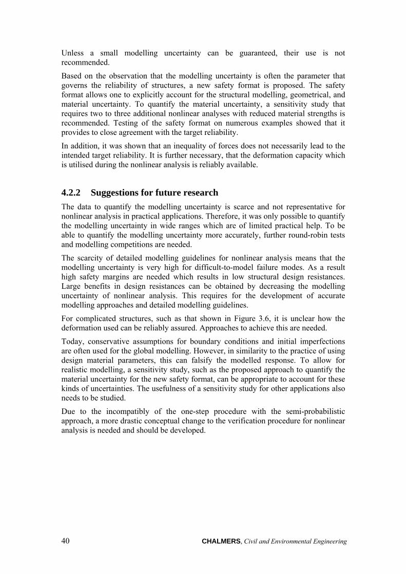
40 CHALMERS, Civil and Environmental Engineering
Unless a small modelling uncertainty can be guaranteed, their use is not recommended.
Based on the observation that the modelling uncertainty is often the parameter that governs the reliability of structures, a new safety format is proposed. The safety format allows one to explicitly account for the structural modelling, geometrical, and material uncertainty. To quantify the material uncertainty, a sensitivity study that requires two to three additional nonlinear analyses with reduced material strengths is recommended. Testing of the safety format on numerous examples showed that it provides to close agreement with the target reliability.
In addition, it was shown that an inequality of forces does not necessarily lead to the intended target reliability. It is further necessary, that the deformation capacity which is utilised during the nonlinear analysis is reliably available.
4.2.2 Suggestions for future research
The data to quantify the modelling uncertainty is scarce and not representative for nonlinear analysis in practical applications. Therefore, it was only possible to quantify the modelling uncertainty in wide ranges which are of limited practical help. To be able to quantify the modelling uncertainty more accurately, further round-robin tests and modelling competitions are needed.
The scarcity of detailed modelling guidelines for nonlinear analysis means that the modelling uncertainty is very high for difficult-to-model failure modes. As a result high safety margins are needed which results in low structural design resistances. Large benefits in design resistances can be obtained by decreasing the modelling uncertainty of nonlinear analysis. This requires for the development of accurate modelling approaches and detailed modelling guidelines.
For complicated structures, such as that shown in Figure 3.6, it is unclear how the deformation used can be reliably assured. Approaches to achieve this are needed.
Today, conservative assumptions for boundary conditions and initial imperfections are often used for the global modelling. However, in similarity to the practice of using design material parameters, this can falsify the modelled response. To allow for realistic modelling, a sensitivity study, such as the proposed approach to quantify the material uncertainty for the new safety format, can be appropriate to account for these kinds of uncertainties. The usefulness of a sensitivity study for other applications also needs to be studied.
Due to the incompatibly of the one-step procedure with the semi-probabilistic approach, a more drastic conceptual change to the verification procedure for nonlinear analysis is needed and should be developed.
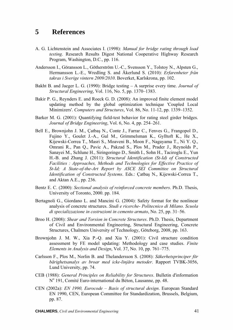
CHALMERS, Civil and Environmental Engineering 41
5 References
A. G. Lichtenstein and Associates I. (1998): Manual for bridge rating through load testing. Research Results Digest National Cooperative Highway Research Program, Washington, D.C., pp. 116.
Andersson I., Göransson L., Götherström U.-C., Svensson Y., Tolstoy N., Alpsten G., Hermansson L.-E., Wredling S. and Åkerlund S. (2010): Erfarenheter från takras i Sverige vintern 2009/2010. Boverket, Karlskrona, pp. 102.
Bakht B. and Jaeger L. G. (1990): Bridge testing – A surprise every time. Journal of Structural Engineering, Vol. 116, No. 5, pp. 1370–1383.
Bakir P. G., Reynders E. and Roeck G. D. (2008): An improved finite element model updating method by the global optimization technique 'Coupled Local Minimizers'. Computers and Structures, Vol. 86, No. 11-12, pp. 1339–1352.
Barker M. G. (2001): Quantifying field-test behavior for rating steel girder bridges. Journal of Bridge Engineering, Vol. 6, No. 4, pp. 254–261.
Bell E., Brownjohn J. M., Çatbaş N., Conte J., Farrar C., Fenves G., Frangopol D., Fujino Y., Goulet J.-A., Gul M., Grimmelsman K., Gylltoft K., He X., Kijewski-Correa T., Masri S., Moaveni B., Moon F., Nagayama T., Ni Y. Q., Omrani R., Pan Q., Pavic A., Pakzad S., Plos M., Prader J., Reynolds P., Sanayei M., Schlune H., Siringoringo D., Smith I., Sohn H., Taciroglu E., Yun H.-B. and Zhang J. (2011): Structural Identification (St-Id) of Constructed Facilities : Approaches, Methods and Technologies for Effective Practice of St-Id; A State-of-the-Art Report by ASCE SEI Committee on Structural Identification of Constructed Systems. Eds.: Çatbaş N., Kijewski-Correa T., and Aktan A.E., pp. 236.
Bentz E. C. (2000): Sectional analysis of reinforced concrete members. Ph.D. Thesis, University of Toronto, 2000. pp. 184.
Bertagnoli G., Giordano L. and Mancini G. (2004): Safety format for the nonlinear analysis of concrete structures. Studi e ricerche- Politecnico di Milano. Scuola di specializzazione in costruzioni in cemento armato, No. 25, pp. 31–56.
Broo H. (2008): Shear and Torsion in Concrete Structures. Ph.D. Thesis, Department of Civil and Environmental Engineering, Structural Engineering, Concrete Structures, Chalmers University of Technology, Göteborg, 2008, pp. 163.
Brownjohn J. M. W., Xia P.-Q. and Xia Y. (2001): Civil structure condition assessment by FE model updating: Methodology and case studies. Finite Elements in Analysis and Design, Vol. 37, No. 10, pp. 761–775.
Carlsson F., Plos M., Norlin B. and Thelandersson S. (2008): Säkerhetsprinciper för bärighetsanalys av broar med icke-linjära metoder. Rapport TVBK-3056, Lund University, pp. 74.
CEB (1988): General Principles on Reliability for Structures. Bulletin d'information No 191, Comité Euro-international du Béton, Lausanne, pp. 48.
CEN (2002a): EN 1990, Eurocode – Basis of structural design. European Standard EN 1990, CEN, European Committee for Standardization, Brussels, Belgium, pp. 87.
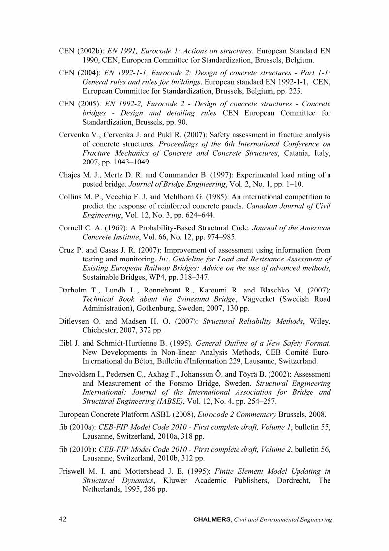
42 CHALMERS, Civil and Environmental Engineering
CEN (2002b): EN 1991, Eurocode 1: Actions on structures. European Standard EN 1990, CEN, European Committee for Standardization, Brussels, Belgium.
CEN (2004): EN 1992-1-1, Eurocode 2: Design of concrete structures - Part 1-1: General rules and rules for buildings. European standard EN 1992-1-1, CEN, European Committee for Standardization, Brussels, Belgium, pp. 225.
CEN (2005): EN 1992-2, Eurocode 2 - Design of concrete structures - Concrete bridges - Design and detailing rules CEN European Committee for Standardization, Brussels, pp. 90.
Cervenka V., Cervenka J. and Pukl R. (2007): Safety assessment in fracture analysis of concrete structures. Proceedings of the 6th International Conference on Fracture Mechanics of Concrete and Concrete Structures, Catania, Italy, 2007, pp. 1043–1049.
Chajes M. J., Mertz D. R. and Commander B. (1997): Experimental load rating of a posted bridge. Journal of Bridge Engineering, Vol. 2, No. 1, pp. 1–10.
Collins M. P., Vecchio F. J. and Mehlhorn G. (1985): An international competition to predict the response of reinforced concrete panels. Canadian Journal of Civil Engineering, Vol. 12, No. 3, pp. 624–644.
Cornell C. A. (1969): A Probability-Based Structural Code. Journal of the American Concrete Institute, Vol. 66, No. 12, pp. 974–985.
Cruz P. and Casas J. R. (2007): Improvement of assessment using information from testing and monitoring. In:. Guideline for Load and Resistance Assessment of Existing European Railway Bridges: Advice on the use of advanced methods, Sustainable Bridges, WP4, pp. 318–347.
Darholm T., Lundh L., Ronnebrant R., Karoumi R. and Blaschko M. (2007): Technical Book about the Svinesund Bridge, Vägverket (Swedish Road Administration), Gothenburg, Sweden, 2007, 130 pp.
Ditlevsen O. and Madsen H. O. (2007): Structural Reliability Methods, Wiley, Chichester, 2007, 372 pp.
Eibl J. and Schmidt-Hurtienne B. (1995). General Outline of a New Safety Format. New Developments in Non-linear Analysis Methods, CEB Comité Euro-International du Béton, Bulletin d'Information 229, Lausanne, Switzerland.
Enevoldsen I., Pedersen C., Axhag F., Johansson Ö. and Töyrä B. (2002): Assessment and Measurement of the Forsmo Bridge, Sweden. Structural Engineering International: Journal of the International Association for Bridge and Structural Engineering (IABSE), Vol. 12, No. 4, pp. 254–257.
European Concrete Platform ASBL (2008), Eurocode 2 Commentary Brussels, 2008.
fib (2010a): CEB-FIP Model Code 2010 - First complete draft, Volume 1, bulletin 55, Lausanne, Switzerland, 2010a, 318 pp.
fib (2010b): CEB-FIP Model Code 2010 - First complete draft, Volume 2, bulletin 56, Lausanne, Switzerland, 2010b, 312 pp.
Friswell M. I. and Mottershead J. E. (1995): Finite Element Model Updating in Structural Dynamics, Kluwer Academic Publishers, Dordrecht, The Netherlands, 1995, 286 pp.
CHALMERS, Civil and Environmental Engineering 43
Grünberg J. (2002): Comments on EN 1990 "Basis of Structural Design", Beuth Verlag, Berlin, 2002, 154 pp.
Hadamard J. (1902): Sur les problèmes aux dérivées partielles et leur signification physique. Bull. Univ. Princeton, Vol. 13, pp. 49–52.
Haldar A. and Mahadevan S. (2000): Reliability Assessment using Stochastic Finite Element Analysis, Wiley, New York, 2000, 328 pp.
Hasofer A. M. and Lind N. C. (1974): Exact and Invariant Second-Moment Code Format. ASCE J Eng Mech Div, Vol. 100, No. EM1, pp. 111–121.
Henriques A. A. R., Calheiros F. and Figueiras J. A. (2002): Safety format for the design of concrete frames. Engineering Computations, Vol. 19, No. 3, pp. 346–363.
Huang D. (2004): Field test and rating of Arlington curved-steel box-girder bridge: Jacksonville, Florida. Transportation Research Record, No. 1892, pp. 178–186.
Huria V., Lee K.-L. and Aktan A. E. (1993): Nonlinear Finite Element Analysis of RC Slab Bridge. Journal of Structural Engineering, Vol. 119, No. 1, January, pp. 88–107.
Huth O., Feltrin G., Maeck J., Kilic N. and Motavalli M. (2005): Damage identification using modal data: Experiences on a prestressed concrete bridge. Journal of Structural Engineering, Vol. 131, No. 12, pp. 1898–1910.
Jaeger T. and Marti P. (2009): Reinforced Concrete Slab Shear Prediction Competition: Entries and Discussion. ACI Structural Journal, Vol. 106, No. 3.
Jaishi B. and Ren W. X. (2005): Structural finite element model updating using ambient vibration test results. Journal of Structural Engineering, Vol. 131, No. 4, pp. 617–628.
Jaishi B. and Ren W. X. (2007): Finite element model updating based on eigenvalue and strain energy residuals using multiobjective optimisation technique. Mechanical Systems and Signal Processing, Vol. 21, No. 5, pp. 2295–2317.
James G. and Karoumi R. (2003): Monitoring of the New Svinesund Bridge, Report 1: Instrumentation of the arch and preliminary results from the construction phase. TRITA-BKN. Rapport 74, Brobyggnad, Royal Institute of Technology (KTH), Stockholm, Sweden, pp. 82.
JCSS. (2001). "Probabilistic Model Code." Joint Committee on Structural Safety, 12th Draft, Zurich.
Johansson H. (2007): Calibration of constitutive models with error control. Ph.D. Thesis, Department of Applied Mechanics, Chalmers University of Technology, Gothenburg, 2007.
Karoumi R. and Andersson A. (2007): Load Testing of the New Svinesund Bridge: Presentation of results and theoretical verification of bridge behaviour. TRITA-BKN Rapport 96, Brobyggnad, Royal Institute of Technology (KTH), Stockholm, Sweden, pp. 173.
König G., Nguyen T. and Ahner C. (1997). Consistent safety format. Non-linear Analysis: Discussion Papers from the Working Party in Commission 1,
44 CHALMERS, Civil and Environmental Engineering
Comité Euro-International du Béton (CEB), Bulletin d' Information 239, Lausanne, 1–16.
König G., Soukhov D. and Jungwirth F. (1998). Sichere Betonproduktion für Stahlbetontragwerke. Fraunhofer IRB Verlag, Stuttgart.
König G., Tue N. and Pommerening D. (1995): Safety Concept for the Application of Nonlinear Analysis in the Design of Concrete Structures, General considerations. CEB–Bulletin d’Information, Vol. 229, pp. 13–31.
Madsen H. O., Krenk S. and Lind N. C. (1986): Methods of Structural Safety, Prentice-Hall, Englewood Cliffs, 1986, 403 pp.
Mancini G. (2002): Non Linear Analysis and Safety Format for Practice. The First fib Congress, Concrete Structures in the 21st Century Osaka, Japan, 2002, pp. 53–58.
Melchers R. E. (1999): Structural reliability analysis and prediction, John Wiley, Chichester ; New York, 1999, 437 pp.
Moses F., Lebet J. P. and Bez R. (1994): Applications of field testing to bridge evaluation. Journal of Structural Engineering, Vol. 120, No. 6, pp. 1745–1762.
Nelder J. A. and Mead R. (1965): A simplex method for function minimization. The Computer Journal, Vol. 7, No. 4, pp. 308–313.
Nowak A. S. and Tharmabala T. (1988): Bridge reliability evaluation using load tests. Journal of Structural Engineering, Vol. 114, No. 10, pp. 2268–2279.
Plos M. and Movaffaghi H. (2004): Finite Element Analysis of the New Svinesund Bridge: Design model conversion and analysis of the arch launching. Report 04:12, Chalmers University of Technology, Structural Engineering and Mechanics, Gothenburg, Sweden, pp. 29.
Rosenbleuth E. and Esteva L. (1972): Reliability bases for some Mexican codes. ACI Publication, Vol. SP-31, pp. 1–41.
Schlune H., Plos M. and Gylltoft K. (2011): Comparative Study of Safety Formats for Nonlinear Finite Element Analysis of Concrete Structures. 11th International Conference on Applications of Statistics and Probability in Civil Engineering, 1-4 August, 2011, Zurich, Switzerland, 2011.
Shahrooz B. M., Ho I. K., Aktan A. E., de Borst R., Blaauwendraad J., van der Veen C., Iding R. H. and Miller R. A. (1994): Nonlinear Finite Element Analysis of Deteriorated RC Slab Bridge. Journal of Structural Engineering, Vol. 120, No. 2, pp. 422–440.
Six M. (2001): Sicherheitskonzept für nichtlinear Traglastverfahren im Betonbau. Ph.D. Thesis, Institut für Massivbau, Technical University Darmstadt, Darmstadt, 2001, pp. 183.
Song H.-W., You D.-W., Byun K.-J. and Maekawa K. (2002): Finite element failure analysis of reinforced concrete T-girder bridges. Engineering Structures, Vol. 24, No. 2, pp. 151–162.
Sustainable Bridges (2007): Guideline for Load and Resistance Assessment of Existing European Railway Bridges: Advices on the use of advanced methods. WP4, pp. 347.
CHALMERS, Civil and Environmental Engineering 45
Ülker-Kaustell M. and Karoumi R. (2006): Monitoring of the New Svinesund Bridge, Report 3: The influence of temperature, wind and damages on the dynamic properties of the bridge. TRITA-BKN. Rapport 99, Brobygnad, Royal Institute of Technology (KTH), Stockholm, Sweden, pp. 75.
USGS. (2011). "Cement Statistics and Information." Mineral Commodity Summaries, U. S. G. Survey, Reston, USA.
van Mier J. G. M. and Ulfkjaer J. P. (2000): Round-Robin analysis of over-reinforced concrete beams – Comparison of results. Materials and Structures, Vol. 33, No. 6, July 2000, pp. 381–390.
Vrouwenvelder A. C. W. M. (2010). "JCSS Workshop on Semi-probabilistic FEM calculations." Delft, The Netherlands.
Waarts P. H. (2000): Structural reliability using finite element analysis. Ph.D. Thesis, Delft University of Technology, Delft University press, The Netherlands, 2000.
Zhang Q. W., Chang T. Y. P. and Chang C. C. (2001): Finite-element model updating for the Kap Shui Mun cable-stayed bridge. Journal of Bridge Engineering, Vol. 6, No. 4, pp. 285–294.

Paper I
Improved bridge evaluation through finite element model updating using static and dynamic measurements. Engineering Structures, Vol. 31, No. 7, pp. 1477–1485.

Engineering Structures 31 (2009) 1477–1485
Contents lists available at ScienceDirect
Engineering Structures
journal homepage: www.elsevier.com/locate/engstruct
Improved bridge evaluation through finite element model updating using staticand dynamic measurementsHendrik Schlune ∗, Mario Plos 1, Kent Gylltoft 2Department of Civil and Environmental Engineering, Division of Structural Engineering, Concrete Structures, Chalmers University of Technology, SE-412 96 Göteborg, Sweden
a r t i c l e i n f o
Article history:Received 12 June 2008Received in revised form18 September 2008Accepted 11 February 2009Available online 10 March 2009
Keywords:Model updatingParameter estimationStructural identificationSystem identificationMulti-responseFinite element method
a b s t r a c t
The potential of combining finite element (FE) analysis with on-site measurement through finite elementmodel updating is indisputable. However, simplified initial models and too few measurements can leadto updated model parameters which conceal inaccurate modelling assumptions rather than improveestimates of the actual structural parameters. Therefore, the methodology proposed aims primarily toeliminate inaccurate modelling simplification by means of manual model refinements before parametersare estimated by non-linear optimization. In addition, multi-response objective functions are introduced,which allow combing different types of measurements to obtain a solid basis for parameter estimation.The proposed methodology was applied to one of the world’s largest single-arch bridges, the newSvinesund Bridge, and disclosed a need to use a non-linear model in order to estimate the structuralparameters more accurately. The resultant model could reproduce the measurements with significantlyimproved accuracy without assigning unrealistic values to model parameters.
© 2009 Elsevier Ltd. All rights reserved.
1. Introduction
Maintenance, upgrading, repair, and replacement of bridgeslead to high costs and considerable disruption of today’s traffic. Foreffective bridge management, accurate and reliable informationabout the safety and condition of bridges is indispensable. Incurrent practice, however, existing bridges are analysed andevaluated by means of highly simplified structural models.This approach is not entirely satisfactory because inevitableuncertainties in material and structural modelling may havesignificant effects on the results of the analysis [1–3]. Structuralmodels that are verified, refined, and tuned with respect to actualmeasurements can reduce these uncertainties and provide a betterbasis for management decisions.A significant amount of research has been done to combine
measurementswith finite element (FE) analysis for the assessmentof bridges. Chajes et al. [4] used strain measurements under truckloading to determine the support restraint and the compositesection properties of a steel-girder-and-concrete-slab bridge.When these findings were introduced into the initial FE model,a substantially higher load carrying capacity could be shown.
∗ Corresponding author. Tel.: +46 (0) 31 772 22 50; fax: +46 (0) 31 772 22 60.E-mail addresses: [email protected] (H. Schlune),
[email protected] (M. Plos), [email protected] (K. Gylltoft).1 Tel.: +46 (0) 31 772 22 44; fax: +46 (0) 31 772 22 60.2 Tel.: +46 (0) 31 772 22 45; fax: +46 (0) 31 772 22 60.
0141-0296/$ – see front matter© 2009 Elsevier Ltd. All rights reserved.doi:10.1016/j.engstruct.2009.02.011
Huang [5] described a method of using strain and deflectionmeasurements to improve the accuracy of FE models. Withoutincluding unreliable effects, such as unintended support restraintwhich may not hold for higher loads or during the entire lifetime,he showed a higher capacity for a box-girder bridge than withconventionalmethods. Enevoldsen et al. [6] changed the stiffnessesof joints manually in an FE model of a truss railway bridge untilgood agreement with measured strains during a train passage wasobtained. The FE model was then used to assess the fatigue life ofthe bridge for higher axle loads. For an overview of bridge ratingbased on load tests and FE analysis see [7].Beside static or quasi-static load tests, modal characteristics
have been extensively used to obtain more information aboutthe response of bridges. Daniell and Macdonald [8] introducedmanual changes to an FEmodel of a cable-stayed bridge to obtain abetter match with eigenfrequencies from ambient vibration tests.However, FE model updating through non-linear optimization ismore common when modal characteristics are used as referencedata; see [9–11].In this study, a methodology is presented which allows
combining static and dynamic measurements with an initial FEmodel to obtain better knowledge of the structural response ofexisting bridges. To avoid obtaining model parameters whichconcealmodelling simplifications the importance ofmanualmodelrefinements is highlighted.In this article, ‘FE model updating’ refers to the complete
procedure of changing an FE model to better correspond toexperimental data. This includes manual model refinements,
1478 H. Schlune et al. / Engineering Structures 31 (2009) 1477–1485
Table 1Methodology for FE model updating.
Steps Purpose
1 Manual model refinements1.1 Remove lower bond assumptions Introduce justified changes1.2 Refine model Disclose the need for model refinements; decrease all types of modelling errors1.3 Conduct parameter study Obtain an overview of model parameter sensitivities; find improved estimates of model parameters
2 Updating through non-linear optimization2.1 Find improved estimates of updating parameters Obtain more accurate model; obtain more accurate estimates of model parameters
3 Model evaluation3.1 Evaluate model parameter changes Evaluate the reliability and accuracy of updated parameters; find possible source for model parameter
changes3.2 Prepare model for further analysis Eliminate model parameter changes that do not hold for the conditions that need to be analysed
a parameter study, and parameter estimation by non-linearoptimization. Furthermore, ‘manual model refinement’ is used todescribe all kinds of changes that are introduced manually tothe model. This term better describes comprehensive changesto the model than does ‘manual tuning’ used by Daniell andMacdonald [8] and Živanović et al. [11] or ‘manual calibration’ usedby Aktan et al. [12].
2. Disagreement between experimental observations and nu-merical predictions
One of the reasons for FE model updating is the need for anaccurate structural model with respect to measurements. If thisis the only goal, FE model updating can be quite simple, as onlysomemodel parameters of the structuralmodel have to be changedwhich lead to improved agreement with the measurements. Insuch a case it is admissible, but not necessary, that the changedmodel parameters be improved estimates of actual structuralparameters as long as they bring about improved agreement withthe measurements.However, when a generally valid FE model that can be used to
analyse untested conditions is sought or when FE model updatingis used as a global non-destructive testing method to estimateuncertain structural parameters, it is important that the updatingprocedure corrects wrong assumptions in the FE model, ratherthan introduces arbitrary changes that make the model agreewith measurements. This is considerably more difficult becausesimplified models, model parameter uncertainties, and inaccuratemeasurements can easily lead to inaccurate estimates of thestructural parameters through FE model updating.In FE model updating, attention is often drawn to changing
model parameters, while less attention is given to other possiblesources of disagreement between measurements and FE analysis.The total modelling error accumulates during the whole finiteelement modelling and analysis process. It starts with theengineer’s decisions about which physical phenomena to includeinto the model. Unavoidable simplifications of the structuralrepresentation concerning the level of detailing, the choice ofelement types and size, boundary conditions, loading, materialparameters, and material models can influence the accuracysignificantly. Furthermore, numerical errors accumulate due toround-off errors and iterative solutions. Robert-Nicoud et al. [13]illustrate the effect of a small modelling simplification on anestimated structural parameter in a simple example.In addition, themeasurement error and signal processing errors
contribute to the total discrepancy between the experimentaland numerical results. The challenges that are associated withmeasuring the response of constructed systems, such as bridges,and the consequences for FE model updating have been describedin [14].The idea underlying structural parameter estimation by FE
model updating is to combine measurements with an a priori FEmodel to gain new information about the structure, typically someof the structural parameters. As the new information is based on
the combination of prior information, namely the measurementsand the initial FE model, the reliability and accuracy of thisnew information strongly depends on the quality of the priorinformation. Therefore, it is essential that the measurement errorand the modelling error are small compared with the error whichis introduced by the model parameters that are updated. Ill-conditioning due to a low sensitivity of the structural response tochanges of model parameters, as observed in [15–17], amplifiesthis problem.
3. Proposed methodology
Due to the previously described difficulties that are associatedwith parameter estimation through FE model updating, two mainimprovements are proposed: manual model refinements beforeparameter estimation through non-linear optimization; and theuse of multiple types of measurements for updating. The steps ofthe proposed methodology are summarized in Table 1.
3.1. Static and dynamic measurements
Finite element model updating can be deceptively simple fora small amount of experimental data and a large number ofuncertain structural parameters [12]. In this instance it is likelythat several non-unique solutions exist. To decrease the risk ofhaving an underdetermined or ill-posed problem, a large amountof experimental data is needed. While either static or dynamicmeasurements are often used for updating, Aktan et al. [12] andCatbas et al. [18] concluded that different types of measurementsare needed when a generally valid model is sought. To obtainimproved estimates of the actual structural parameters of abridge, it is important that the uncertain structural parametersdetermine the choice of measurements, not the reverse. To finda set of measurements that can be used to estimate the mainuncertain structural parameters, it can be helpful to simulate themodel updating procedure before undertaking expensive on-sitemeasurements.Furthermore, it is desirable to choose measurement types and
loading conditions which are relevant to the final purpose of theupdated FE model. This reduces the consequences of inaccuratelyestimated structural parameters through FE model updatingand decreases the uncertainty associated with extrapolating thefinding to other loading conditions.Compared to static measurements, modal characteristics have
the advantage of containing information about the global responseof bridges. This makes them less sensitive to local structural pa-rameters. The number of identifiable modes limits the informationthat can be gained about the response of a bridge. The number ofstatic measurements, typically strains, forces, displacements, andinclinations, under known loads is limited only by the number ofavailable sensors. As measured strains and forces are more sensi-tive to the response in their vicinity, they are better suited to de-termine local parameters. On the other hand a dense net of sensorsis requiredwhen information about the global response of a bridge
H. Schlune et al. / Engineering Structures 31 (2009) 1477–1485 1479
is sought. For these reasons, Aktan et al. [12] and Catbas et al. [18]used the first modal characteristics to update the boundary con-ditions and then static measurements to update the local modelparameters.
3.2. Manual model refinements
To obtain an accurate FE model that can capture all importantphysical effects and allows for estimation of uncertain structuralparameters, manual model refinements can be crucial. Theproposed procedure successively reduces the modelling errorsof an initial FE model, thereby reducing the risk of concealingthe initial modelling simplifications by inaccurately estimatedstructural parameters. The strength of manual model refinementsis that they can be used to decrease all types of modellingerrors, while the strength of FE model updating by non-linearoptimization lies in tuning uncertain model parameters. Manualmodel refinements can be done in three steps; however, it may benecessary to apply the second and third steps alternately.When FE models are used for the design or assessment
of bridges, simplifications and assumptions ‘on the safe side’are appropriate. However, the FE models used for FE modelupdating should be as accurate as possible. Therefore, all lowerbond assumptions should be replaced by realistic assumptionsin a first step. To avoid introducing additional modelling errors,it is recommended to first base all changes on engineeringcalculations without taking into account the agreement betweenthe measurements and the FE analysis.In a second step, the FE model can be changed according to
agreement between the FE analysis results and themeasurements.By comparing the residuals for different load cases, measurementlocations and sensor types, invalid or inaccurate assumptionsin the FE model can be disclosed. An iterative trial and errorprocedure based on engineering judgement can be used tointroduce realistic changes into themodel. As boundary conditionsand joint properties often have a high influence on the FEanalysis results, their representation in the FE model shouldbe reviewed. Furthermore, one can check whether additionalphysical phenomena have to be introduced into the FE modelto obtain a more realistic description of reality. This also leads,through experience, to an improved understanding of the physicalphenomena which have to be included when modelling commonbridge types and, hence, to more accurate a priori models.In the third step, the model and the measurements can be
combined to gain more information about uncertain structuralparameters. This can be done by changing uncertain modelparameters until improved agreement between the numerical andexperimental response is obtained. Another way is to conduct aparameter study by formulating an index of discrepancy, calledthe objective function, and plotting the value of the objectivefunction for parameter variations. An advantage of this procedureis that it gives an idea of the shape of the objective functions,which makes it easier to assess the reliability of the estimatedparameters. If the agreement of the model with measurements issatisfactory, a critical assessment of the model should be madebefore it can be used for further analysis; see Section 3.4. Forfurther improvements of the model and the estimated structuralparameters, FE model updating through non-linear optimizationcan be utilized. An advantage of manually improving estimatesof the structural parameters is that a better starting point forthe optimization algorithm is obtained, which reduces the risk ofgetting stuck in local minima.
3.3. FE model updating through non-linear optimization
An increasing number of model parameters are impractical totune manually. Therefore, optimization algorithms are commonlyused to find model parameters that make the FE model agreebetter with measurements. Finite element model updating by
non-linear optimization consists of three main components,namely the choice of updating parameters, the objective (or cost)function, and the optimization algorithm.Updating parameters are the model parameters that are
changed by the optimization algorithm to minimize the objectivefunction. To increase the sensitivity ofmodel parameters, groupingof those which show a high correlation can be done. Whenestimating the uncertainty of possible updating parameters, onemust be aware of the distinction between the certainty of theelastic modulus of a steel beam, for example, and the uncertaintyof the elastic modulus of the bridge deck girder, which is used asan updating parameter. In the first example the elastic modulusis a material parameter which is accurately known; see [19]. In thesecond, the elasticmodulus is used as a parameter which describesthe stiffness changes of the bridge deck in all directions. In thisinstance it is used to summarize effects, such as the railing systemand the asphalt layer, on the structural performance of the bridgedeck girder, which leads to higher uncertainty.Optimization algorithms are typically required to be stable and
fast. The Gauss–Newton algorithm is probably the most oftenused algorithm for FE model updating; see e.g. [20]. Teughelsand De Roeck [21] applied the Gauss–Newton method witha trust region strategy to improve stability. Gentile [22] usedRosenbrock’s methods; global optimization algorithms have alsobeen applied [23].The objective function is an index of discrepancy between the
FE analysis results and the measurements. As FE model updatingby non-linear optimization using static measurements has seldombeen applied, experience in the choice of an appropriate objectivefunction is still limited. When eigenfrequencies are used to updatean FE model, the sum of squared differences or the sum of squaredrelative differences has usually been used:
J1 =m∑i=1
(zni − zei)2 = (zn − ze)T(zn − ze) (1)
J2 =m∑i=1
(zni − zeizei
)2= (zn − ze)TW2(zn − ze), (2)
where zn and ze are vectors with numerical and experimentaleigenfrequencies, respectively, m is the number of eigenfrequen-cies, and W2 is a diagonal matrix with the squared reciprocals ofthe experimental eigenfrequencies as diagonal elements.When different types of measurements contribute to the
objective function, it is important that they are unit-less.Normalization is therefore required to assure that the contributionto the objective function is not dependent on the units chosen.Eq. (2) fulfils this demand and could thus be used as a multi-response objective function when zn and ze are changed intovectors containing different types of numerical and experimentalresponses. Problems arise when the normalization factors areclose to zero. In this instance the objective function can becomedominated by one or a few terms. When eigenfrequencies areused exclusively in the objective function, this problem does notoccur. However,whenmeasured displacements, strains, and forcesunder various types of loadings are used, there is a risk thatsome measured responses will be very small compared with thedifference between the numerical and measured responses.Bell et al. [24] chose the difference between the measured and
the numerical response of the initial model as a normalizationparameter. This can cause the objective function to be dominatedby a few terms, when some measured and numerical responseshappen to agree very well initially.A way of taking the significance of different kinds of measure-
ments into account and obtaining dimensionless terms is to use
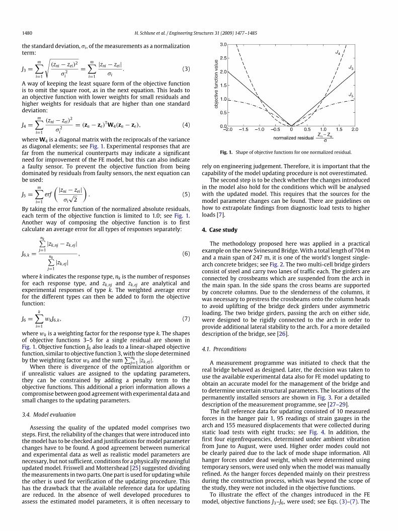
1480 H. Schlune et al. / Engineering Structures 31 (2009) 1477–1485
the standard deviation, σi, of themeasurements as a normalizationterm:
J3 =m∑i=1
√(zni − zei)2
σ 2i=
m∑i=1
|zni − zei|σi
. (3)
A way of keeping the least square form of the objective functionis to omit the square root, as in the next equation. This leads toan objective function with lower weights for small residuals andhigher weights for residuals that are higher than one standarddeviation:
J4 =m∑i=1
(zni − zei)2
σ 2i= (zn − ze)TW4(zn − ze), (4)
whereW4 is a diagonal matrix with the reciprocals of the varianceas diagonal elements; see Fig. 1. Experimental responses that arefar from the numerical counterparts may indicate a significantneed for improvement of the FE model, but this can also indicatea faulty sensor. To prevent the objective function from beingdominated by residuals from faulty sensors, the next equation canbe used:
J5 =m∑i=1
erf(|zni − zei|
σi√2
). (5)
By taking the error function of the normalized absolute residuals,each term of the objective function is limited to 1.0; see Fig. 1.Another way of composing the objective function is to firstcalculate an average error for all types of responses separately:
J6,k =
nk∑j=1|zk,nj − zk,ej|
nk∑j=1|zk,ej|
, (6)
where k indicates the response type, nk is the number of responsesfor each response type, and zk,nj and zk,ej are analytical andexperimental responses of type k. The weighted average errorfor the different types can then be added to form the objectivefunction:
J6 =k∑i=1
wkJ6,k, (7)
wherewk is a weighting factor for the response type k. The shapesof objective functions 3–5 for a single residual are shown inFig. 1. Objective function J6 also leads to a linear-shaped objectivefunction, similar to objective function 3, with the slope determinedby the weighting factorwk and the sum
∑nkj=1 |zk,ej|.
When there is divergence of the optimization algorithm orif unrealistic values are assigned to the updating parameters,they can be constrained by adding a penalty term to theobjective functions. This additional a priori information allows acompromise between good agreementwith experimental data andsmall changes to the updating parameters.
3.4. Model evaluation
Assessing the quality of the updated model comprises twosteps. First, the reliability of the changes that were introduced intothemodel has to be checked and justifications formodel parameterchanges have to be found. A good agreement between numericaland experimental data as well as realistic model parameters arenecessary, but not sufficient, conditions for a physicallymeaningfulupdated model. Friswell and Mottershead [25] suggested dividingthemeasurements in twoparts. One part is used for updatingwhilethe other is used for verification of the updating procedure. Thishas the drawback that the available reference data for updatingare reduced. In the absence of well developed procedures toassess the estimated model parameters, it is often necessary to
Fig. 1. Shape of objective functions for one normalized residual.
rely on engineering judgement. Therefore, it is important that thecapability of the model updating procedure is not overestimated.The second step is to be check whether the changes introduced
in the model also hold for the conditions which will be analysedwith the updated model. This requires that the sources for themodel parameter changes can be found. There are guidelines onhow to extrapolate findings from diagnostic load tests to higherloads [7].
4. Case study
The methodology proposed here was applied in a practicalexample on the new Svinesund Bridge.With a total length of 704mand a main span of 247 m, it is one of the world’s longest single-arch concrete bridges; see Fig. 2. The two multi-cell bridge girdersconsist of steel and carry two lanes of traffic each. The girders areconnected by crossbeams which are suspended from the arch inthe main span. In the side spans the cross beams are supportedby concrete columns. Due to the slenderness of the columns, itwas necessary to prestress the crossbeams onto the column headsto avoid uplifting of the bridge deck girders under asymmetricloading. The two bridge girders, passing the arch on either side,were designed to be rigidly connected to the arch in order toprovide additional lateral stability to the arch. For a more detaileddescription of the bridge, see [26].
4.1. Preconditions
A measurement programme was initiated to check that thereal bridge behaved as designed. Later, the decision was taken touse the available experimental data also for FE model updating toobtain an accurate model for the management of the bridge andto determine uncertain structural parameters. The locations of thepermanently installed sensors are shown in Fig. 3. For a detaileddescription of the measurement programme, see [27–29].The full reference data for updating consisted of 10 measured
forces in the hanger pair 1, 95 readings of strain gauges in thearch and 155 measured displacements that were collected duringstatic load tests with eight trucks; see Fig. 4. In addition, thefirst four eigenfrequencies, determined under ambient vibrationfrom June to August, were used. Higher order modes could notbe clearly paired due to the lack of mode shape information. Allhanger forces under dead weight, which were determined usingtemporary sensors, were used only when the model was manuallyrefined. As the hanger forces depended mainly on their prestressduring the construction process, which was beyond the scope ofthe study, they were not included in the objective functions.To illustrate the effect of the changes introduced in the FE
model, objective functions J3–J6, were used; see Eqs. (3)–(7). The
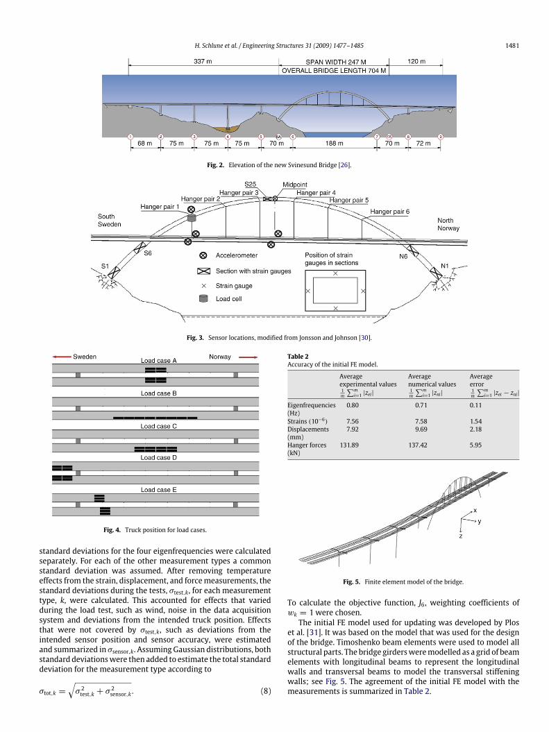
H. Schlune et al. / Engineering Structures 31 (2009) 1477–1485 1481
Fig. 2. Elevation of the new Svinesund Bridge [26].
Fig. 3. Sensor locations, modified from Jonsson and Johnson [30].
Fig. 4. Truck position for load cases.
standard deviations for the four eigenfrequencies were calculatedseparately. For each of the other measurement types a commonstandard deviation was assumed. After removing temperatureeffects from the strain, displacement, and forcemeasurements, thestandard deviations during the tests, σtest,k, for each measurementtype, k, were calculated. This accounted for effects that variedduring the load test, such as wind, noise in the data acquisitionsystem and deviations from the intended truck position. Effectsthat were not covered by σtest,k, such as deviations from theintended sensor position and sensor accuracy, were estimatedand summarized in σsensor,k. Assuming Gaussian distributions, bothstandard deviationswere then added to estimate the total standarddeviation for the measurement type according to
σtot,k =
√σ 2test,k + σ
2sensor,k. (8)
Table 2Accuracy of the initial FE model.
Averageexperimental values
Averagenumerical values
Averageerror
1m
∑mi=1 |zei|
1m
∑mi=1 |zni|
1m
∑mi=1 |zei − zni|
Eigenfrequencies(Hz)
0.80 0.71 0.11
Strains (10−6) 7.56 7.58 1.54Displacements(mm)
7.92 9.69 2.18
Hanger forces(kN)
131.89 137.42 5.95
Fig. 5. Finite element model of the bridge.
To calculate the objective function, J6, weighting coefficients ofwk = 1 were chosen.The initial FE model used for updating was developed by Plos
et al. [31]. It was based on the model that was used for the designof the bridge. Timoshenko beam elements were used to model allstructural parts. The bridge girdersweremodelled as a grid of beamelements with longitudinal beams to represent the longitudinalwalls and transversal beams to model the transversal stiffeningwalls; see Fig. 5. The agreement of the initial FE model with themeasurements is summarized in Table 2.
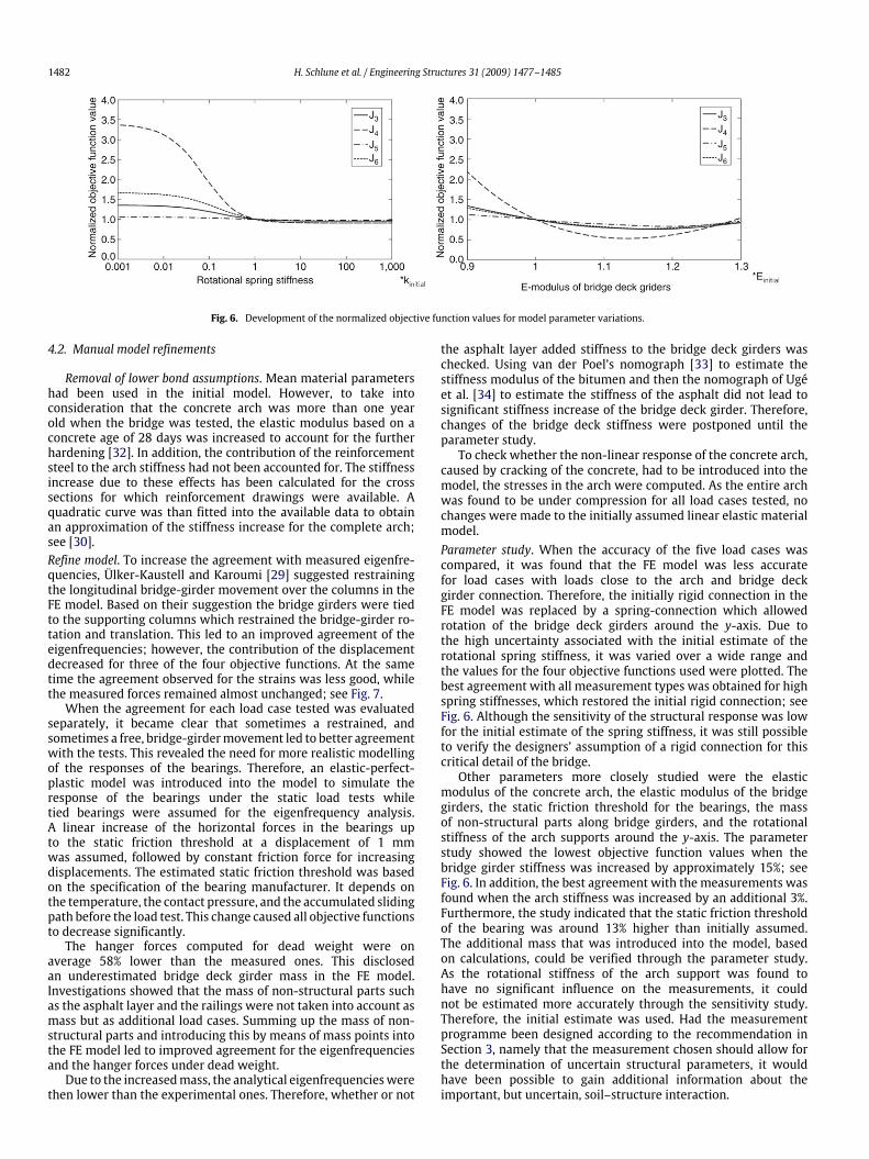
1482 H. Schlune et al. / Engineering Structures 31 (2009) 1477–1485
Fig. 6. Development of the normalized objective function values for model parameter variations.
4.2. Manual model refinements
Removal of lower bond assumptions. Mean material parametershad been used in the initial model. However, to take intoconsideration that the concrete arch was more than one yearold when the bridge was tested, the elastic modulus based on aconcrete age of 28 days was increased to account for the furtherhardening [32]. In addition, the contribution of the reinforcementsteel to the arch stiffness had not been accounted for. The stiffnessincrease due to these effects has been calculated for the crosssections for which reinforcement drawings were available. Aquadratic curve was than fitted into the available data to obtainan approximation of the stiffness increase for the complete arch;see [30].Refine model. To increase the agreement with measured eigenfre-quencies, Ülker-Kaustell and Karoumi [29] suggested restrainingthe longitudinal bridge-girder movement over the columns in theFE model. Based on their suggestion the bridge girders were tiedto the supporting columns which restrained the bridge-girder ro-tation and translation. This led to an improved agreement of theeigenfrequencies; however, the contribution of the displacementdecreased for three of the four objective functions. At the sametime the agreement observed for the strains was less good, whilethe measured forces remained almost unchanged; see Fig. 7.When the agreement for each load case tested was evaluated
separately, it became clear that sometimes a restrained, andsometimes a free, bridge-girdermovement led to better agreementwith the tests. This revealed the need for more realistic modellingof the responses of the bearings. Therefore, an elastic-perfect-plastic model was introduced into the model to simulate theresponse of the bearings under the static load tests whiletied bearings were assumed for the eigenfrequency analysis.A linear increase of the horizontal forces in the bearings upto the static friction threshold at a displacement of 1 mmwas assumed, followed by constant friction force for increasingdisplacements. The estimated static friction threshold was basedon the specification of the bearing manufacturer. It depends onthe temperature, the contact pressure, and the accumulated slidingpath before the load test. This change caused all objective functionsto decrease significantly.The hanger forces computed for dead weight were on
average 58% lower than the measured ones. This disclosedan underestimated bridge deck girder mass in the FE model.Investigations showed that the mass of non-structural parts suchas the asphalt layer and the railings were not taken into account asmass but as additional load cases. Summing up the mass of non-structural parts and introducing this by means of mass points intothe FE model led to improved agreement for the eigenfrequenciesand the hanger forces under dead weight.Due to the increasedmass, the analytical eigenfrequencieswere
then lower than the experimental ones. Therefore, whether or not
the asphalt layer added stiffness to the bridge deck girders waschecked. Using van der Poel’s nomograph [33] to estimate thestiffness modulus of the bitumen and then the nomograph of Ugéet al. [34] to estimate the stiffness of the asphalt did not lead tosignificant stiffness increase of the bridge deck girder. Therefore,changes of the bridge deck stiffness were postponed until theparameter study.To check whether the non-linear response of the concrete arch,
caused by cracking of the concrete, had to be introduced into themodel, the stresses in the arch were computed. As the entire archwas found to be under compression for all load cases tested, nochanges were made to the initially assumed linear elastic materialmodel.Parameter study. When the accuracy of the five load cases wascompared, it was found that the FE model was less accuratefor load cases with loads close to the arch and bridge deckgirder connection. Therefore, the initially rigid connection in theFE model was replaced by a spring-connection which allowedrotation of the bridge deck girders around the y-axis. Due tothe high uncertainty associated with the initial estimate of therotational spring stiffness, it was varied over a wide range andthe values for the four objective functions used were plotted. Thebest agreement with all measurement types was obtained for highspring stiffnesses, which restored the initial rigid connection; seeFig. 6. Although the sensitivity of the structural response was lowfor the initial estimate of the spring stiffness, it was still possibleto verify the designers’ assumption of a rigid connection for thiscritical detail of the bridge.Other parameters more closely studied were the elastic
modulus of the concrete arch, the elastic modulus of the bridgegirders, the static friction threshold for the bearings, the massof non-structural parts along bridge girders, and the rotationalstiffness of the arch supports around the y-axis. The parameterstudy showed the lowest objective function values when thebridge girder stiffness was increased by approximately 15%; seeFig. 6. In addition, the best agreement with the measurements wasfound when the arch stiffness was increased by an additional 3%.Furthermore, the study indicated that the static friction thresholdof the bearing was around 13% higher than initially assumed.The additional mass that was introduced into the model, basedon calculations, could be verified through the parameter study.As the rotational stiffness of the arch support was found tohave no significant influence on the measurements, it couldnot be estimated more accurately through the sensitivity study.Therefore, the initial estimate was used. Had the measurementprogramme been designed according to the recommendation inSection 3, namely that the measurement chosen should allow forthe determination of uncertain structural parameters, it wouldhave been possible to gain additional information about theimportant, but uncertain, soil–structure interaction.
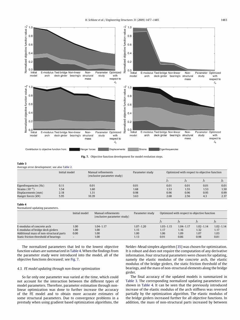
H. Schlune et al. / Engineering Structures 31 (2009) 1477–1485 1483
Fig. 7. Objective function development for model evolution steps.
Table 3Average error development; see also Table 2.
Initial model Manual refinements(exclusive parameter study)
Parameter study Optimized with respect to objective function
J3 J4 J5 J6
Eigenfrequencies (Hz) 0.11 0.01 0.01 0.01 0.01 0.01 0.01Strains (10−6) 1.54 1.60 1.68 1.53 1.55 1.53 1.50Displacements (mm) 2.18 1.31 0.98 0.96 0.96 0.95 0.99Hanger forces (kN) 5.95 10.39 3.63 2.68 2.56 4.3 2.37
Table 4Normalized updating parameters.
Initial model Manual refinements(exclusive parameter study)
Parameter study Optimized with respect to objective function
J3 J4 J5 J6
E-modulus of concrete arch 1.00 1.04–1.17 1.07–1.20 1.03–1.15 1.04–1.17 1.02–1.14 1.02–1.14E-modulus of bridge deck girders 1.00 1.00 1.15 1.17 1.16 1.32 1.17Additional mass of non-structural parts 0.00 1.00 1.00 1.06 1.09 1.07 1.03Static friction threshold of bearings – 1.00 1.13 0.91 0.86 0.98 0.81
The normalized parameters that led to the lowest objectivefunction values are summarized in Table 4.When the findings fromthe parameter study were introduced into the model, all of theobjective functions decreased; see Fig. 7.
4.3. FE model updating through non-linear optimization
So far only one parameter was varied at the time, which couldnot account for the interaction between the different types ofmodel parameters. Therefore, parameter estimation through non-linear optimization was done to further increase the accuracyof the FE model and to obtain more accurate estimates ofsome structural parameters. Due to convergence problems in aprestudy when using gradient based optimization algorithms, the
Nelder–Mead simplex algorithm [35] was chosen for optimization.It is robust and does not require the computation of any derivativeinformation. Four structural parameters were chosen for updating,namely the elastic modulus of the concrete arch, the elasticmodulus of the bridge girders, the static friction threshold of thebearings, and themass of non-structural elements along the bridgegirder.The final accuracy of the updated models is summarized in
Table 3. The corresponding normalized updating parameters areshown in Table 4. It can be seen that the previously introducedincrease of the elastic modulus of the arch stiffness was reversedpartially by the optimization algorithm. The elastic modulus ofthe bridge girders increased further for all objective functions. Inaddition, the mass of non-structural parts increased by between
1484 H. Schlune et al. / Engineering Structures 31 (2009) 1477–1485
3% and 9% and the static friction threshold of the bearingsdecreased by between 13% and 28%. Even though the sametendency of updating parameter changes could be observed, theirfinal normalized values differed with up to 0.17 depending on thechosen objective function. The optimization algorithm decreasedobjective functions J3 and J6 by approximately 11%, J4 by 31%, andJ5 by less than 6% compared to the parameter study. These are onlysmall improvements compared to the manual model refinements,despite substantial changes to the updating parameters. The lowsensitivity of the objective functions with respect to the updatingparameter changes, in combination with the high influenceof model simplification, highlights the difficulties which areassociated with structural parameter estimation by FE modelupdating. The final normalized objective function values arepresented in Fig. 7.Although all objective functions clearly show increased model
accuracy with the changes introduced, their development is quitedifferent. Objective function J4 drops to 2.4% of the initial valuewhile objective function J5 decreases only to 69%. The highdrop of J4 is mainly due to the improved agreement of thesecond eigenfrequency, which contributes to more than 80% ofthe objective function value before a restrained bridge girdermovement is introduced into the model. On the other hand,the second eigenfrequency adds less than 1% to the value ofobjective function J5 for the first twomodel evolution steps. A goodcompromise between these two extremes is objective function J3.A descriptive method of expressing the model discrepancy can beobtained by objective function J6, which can be interpreted as theaverage error for all of the measurement types.
4.4. Model evaluation
All of the changes introduced as manual model refinements be-fore the parameter study could be reasoned. Thus, high confidencein the changes introduced was achieved. The parameter changesthat were based on the parameter study or the optimization al-gorithm are more uncertain. All updating parameters remainedwithin realistic ranges without introducing constraints.The highest uncertainty was associated with the stiffness
increase of the bridge girders, which was derived from theparameter study. The reason for this has to be carefully analysedbefore it can be relied on in further analysis. A possible source foradditional stiffness is the railing system.In addition, the static friction of the bearings was shown to
have a significant effect on the measured properties. In particular,the eigenfrequency agreement improvedwhen a restrained bridgedeck girdermovementwas assumed.However, the load test clearlyshowed that the bearings move under higher horizontal forces.Therefore, it can be questioned whether a restrained bridge girdermovement can be assumed for higher excitations such as strongwinds or earthquakes. For analysis under static loads, one cannotrely on the static friction in the bearings, as it may not hold for alonger period of time due to thermal changes or excitation causedby passing vehicles.
5. Discussion
In Table 3 and Fig. 7 it can be seen that the agreement of themodel with the strain measurements remains almost unchangedfor all model evolution steps. A plausible reason is that the strainsensors have been placed in or close to disturbed regions. Thiscould not been accounted for by the beam elements which havebeen used in the model. Furthermore, other local effects like theelastic modulus variation of the concrete or the reinforcementarrangement around the strain sensors generally limit the accuracyof strain measurements in concrete and hence their value formodel updating.For the other measurements types a significant better agree-
ment was obtained through FE model updating without assigningunrealistic values to the updating parameters. However, a certain
inaccuracy of the model remained. To further increase the agree-ment of themodel with themeasurements, a less restrictive choiceof updating parameters was tested. For example, by using two up-dating parameter for the arch stiffness, one for the arch bases, oneat the crown, and quadratic interpolation in between, further de-creasing objective functions could be obtained. However, due tothe unrealistic values that were assigned to the concrete crosssections, it is believed that the updating algorithm compensatesfor the model simplification or measurement errors by unrealis-tic model parameters, instead of finding improved estimates of theactual structural parameters.It was also possible to obtain a more accurate model with
respect to one type of measurements or to selected parts of themeasurements when the others were excluded from the objectivefunction. The challenge however was to obtain a model that couldreproduce all 264 measured values with reasonable accuracy.
6. Conclusions
A methodology for FE model updating for improved bridgeevaluation has been proposed and applied. Important aspects likethe choice of measurements, model simplifications, the accuracyand reliability of updated parameters, and the analysis of untestedloading conditions have been included.While the focus of FE model updating is usually on tuning
model parameters, this article highlights the importance ofother modelling errors. Manual model refinements prior to FEmodel updating by non-linear optimization was shown to bedecisive for the success of the case study conducted. The manualmodel refinements decreased the initial modelling error throughphysically justified changes and allowed thedetection of importantphysical phenomena which had to be introduced into the model.This reduced the risk of compensating for modelling errors bymeaningless changes to updating parameters.Furthermore, it was shown that FE model updating can be
applied to non-linear models of real bridges. Besides the slightlyincreased computational time, no problems were encounteredafter introducing the non-linear bearing response into the model.Four multi-response objective functions for FE model updating
were proposed and tested. It was shown that improved accuracyfor eigenfrequency calculations does not necessarily lead to animproved model for static analysis. The combination of numerousand diverse kinds of measurements should preferably be usedwhen a generally valid and accurate model is sought. As a differentbearing behaviour was observed under ambient excitation andduring the load tests, it was not possible to update the boundaryconditions through modal characteristics and then use the sameboundary conditions for static analysis.
Acknowledgements
The authorswould like to express their gratitude to the SwedishRoad and Railway Administration, Vägverket and Banverket, fortheir financial support and to Raid Karoumi, Professor at KTH,Mahir Ülker-Kaustell, Ph.D. student at KTH, Fredrik Jonsson, M.Sc.,and David Johnson, M.Sc., for their help.
References
[1] Huria V, Lee K-L, Aktan AE. Nonlinear finite element analysis of RC slab bridge.J Struct Eng 1993;119(1):88–107.
[2] Shahrooz BM, Ho IK, Aktan AE, de Borst R, Blaauwendraad J, van der Veen C,et al. Nonlinear finite element analysis of deteriorated RC slab bridge. J StructEng 1994;120(2):422–40.
[3] Song H-W, You D-w, Byun K-J, Maekawa K. Finite element failure analysis ofreinforced concrete T-girder bridges. Eng Struct 2002;24(2):151–62.
[4] Chajes MJ, Mertz DR, Commander B. Experimental load rating of a postedbridge. J Bridge Eng 1997;2(1):1–10.
H. Schlune et al. / Engineering Structures 31 (2009) 1477–1485 1485
[5] Huang D. Field test and rating of Arlington curved-steel box-girder bridge:Jacksonville, Florida. Transportation Research Record 2004;1892:178–86.
[6] Enevoldsen I, Pedersen C, Axhag F, Johansson Ö, Töyrä B. Assessmentand measurement of the Forsmo Bridge Sweden Structural EngineeringInternational. J Internat Assoc Bridge Struct Eng (IABSE) 2002;12(4):254–257.
[7] Lichtenstein AG, Associates I. Manual for bridge rating through load testing.In: Program NCHR, editor. Research results digest. WA: TransportationResearch Board; 1998. p. 116.
[8] Daniell WE, Macdonald JHG. Improved finite element modelling of a cable-stayed bridge through systematic manual tuning. Eng Struct 2007;29(3):358–71.
[9] Brownjohn JMW, Xia P-Q. Dynamic assessment of curved cable-stayed bridgeby model updating. J Struct Eng 2000;126(2):252–60.
[10] Zhang QW, Chang TYP, Chang CC. Finite-element model updating for the KapShui Mun cable-stayed bridge. J Bridge Eng 2001;6(4):285–94.
[11] Živanović S, Pavic A, Reynolds P. Finite element modelling and updating of alively footbridge: The complete process. J Sound Vib 2007;301(1-2):126–45.
[12] Aktan E, Catbas N, Turer A, Zhang Z. Structural identification: Analyticalaspects. J Struct Eng 1998;124(7):817–29.
[13] Robert-Nicoud Y, Raphael B, Smith IFC. System identification through modelcomposition and stochastic search. J Comput Civil Eng 2005;19(3):239–47.
[14] Moon FL, Aktan AE. Impacts of epistemic (bias) uncertainty on structuralidentification of constructed (civil) systems. Shock Vib Digest 2006;38(5):399–420.
[15] Teughels A, De Roeck G. Damage assessment of the Z24 bridge by FE modelupdating. Key Eng Mater 2003;245–346:19–26.
[16] Huth O, Feltrin G, Maeck J, Kilic N, Motavalli M. Damage identification usingmodal data: Experiences on a prestressed concrete bridge. J Struct Eng 2005;131(12):1898–910.
[17] Brownjohn JMW, Xia P-Q, Xia Y. Civil structure condition assessment by FEmodel updating: Methodology and case studies. Finite Elem Anal Des 2001;37(10):761–75.
[18] Catbas FN, Ciloglu SK, Hasancebi O, Grimmelsman K, Aktan AE. Limitationsin structural identification of large constructed structures. J Struct Eng 2007;133(8):1051–66.
[19] Joint Committee on Structural Safety (JCSS). Probabilistic model code. Internetpublication; 2001.
[20] Brownjohn JMW, Moyo P, Omenzetter P, Lu Y. Assessment of highway bridgeupgrading by dynamic testing and finite-elementmodel updating. J Bridge Eng2003;8(3):162–72.
[21] Teughels A, De Roeck G. Structural damage identification of the highwaybridge Z24 by FE model updating. J Sound Vib 2004;278(3):589–610.
[22] Gentile C. Modal and structural identification of a R.C. arch bridge. Struct EngMech 2006;22(1):53–70.
[23] Levin RI, Lieven NAJ. Dynamic finite element model updating using simulatedannealing and genetic algorithms. Mech Syst Signal Process 1998;12(1):91–120.
[24] Bell ES, Sanayei M, Javdekar CN, Slavsky E. Multiresponse parameterestimation for finite-element model updating using nondestructive test data.J Struct Eng 2007;133(8):1067–79.
[25] Friswell MI, Mottershead JE. Finite element model updating in structuraldynamics. Dordrecht, The Netherlands: Kluwer Academic Publishers; 1995.
[26] Darholm T, Lundh L, Ronnebrant R, Karoumi R, Blaschko M. Technical bookabout the Svinesund bridge. Göteborg (Sweden): Vägverket (Swedish RoadAdministration); 2007.
[27] James G, Karoumi R. Monitoring of the new Svinesund bridge. Report 1:Instrumentation of the arch and preliminary results from the constructionphase. Stockholm (Sweden): KTH Byggvetenskap. 2003. p. 82.
[28] Karoumi R, Andersson A. Load testing of the new Svinesund bridge:presentation of results and theoretical verification of bridge behaviour.Stockholm (Sweden): KTH Byggvetenskap, 2007. p. 173.
[29] Ülker-Kaustell M, Karoumi R. Monitoring of the new Svinesund bridge. Report3: The influence of temperature, wind and damages on the dynamic propertiesof the bridge. Stockholm (Sweden): KTH Byggvetenskap; 2006. p. 75.
[30] Jonsson F, Johnson D. Finite element model updating of the new Svinesundbridge. Civil and Environmental Engineering. Göteborg (Sweden): ChalmersUniversity of Technology, Civil and Environmental Engineering; 2007. p. 228.
[31] Plos M, Movaffaghi H. Finite element analysis of the new Svinesund bridge:Design model conversion and analysis of the arch launching. Göteborg,(Sweden): Chalmers University of Technology, Structural Engineering andMechanics; 2004. p. 29.
[32] CEN. Eurocode 2: Design of concrete structures — Part 1-1: General rulesand rules for buildings. Brussels (Belgium): CEN, European Committee forStandardization; 2004. p. 225.
[33] Van der Poel C. A general system describing the visco-elastic properties ofbitumen and its relation to routine test data. J Appl Chemistry 1954;4:221–36.
[34] Ugé P, Gest G, Gravois A, Bonnaure F. Nouvelle méthode de calcul du modulecomplexedesmélanges bitumineux (Anewmethodof calculating the complexmodulus of bitumen mixtures). Cah Groupe Fr Rheol 1978;4(6):259–80.
[35] Nelder JA, Mead R. A simplex method for function minimization. Comput J1965;7(4):308–13.

Paper II
Safety Formats for Nonlinear Analysis of Concrete Structures.
Provisionally accepted for publication in Magazine of Concrete Research April 2011.

II-1
Safety Formats for Nonlinear Analysis of Concrete Structures
Hendrik Schlune, Mario Plos, Kent Gylltoft
Department of Civil and Environmental Engineering,
Chalmers University of Technology,
SE-412 96 Gothenburg,
Sweden
Abstract For realistic modelling of reinforced concrete structures, nonlinear models are often inevitable, which raises the question of an appropriate safety format for nonlinear analysis. This article gives an overview of available safety formats and discusses their advantages and disadvantages. An analysis of available round robin tests and modelling competitions shows that current safety formats do not properly account for the modelling uncertainty of nonlinear analysis. Based on this observation a new safety format was proposed which allows one to explicitly account for the modelling uncertainty. To avoid any interaction of the modelled response with the safety format, the mean in situ material parameters should be used in the nonlinear analysis and a resistance safety factor is used to assure the intended reliability level. The application of the new safety format to beam sections loaded in bending showed that it offers a reliability level that is in good agreement with the target reliability.
Keywords: nonlinear analysis, model uncertainty, concrete, safety format, reliability
Notation area of the concrete section
nominal geometrical parameters
, area of the longitudinal reinforcement
width of a beam step size parameter effective depth of a beam
concrete compressive strength used in the nonlinear analysis according to EN 1992-2 mean concrete compressive strength of specially cured cylinders
, mean in situ concrete compressive strength
characteristic concrete compressive strength
, characteristic in situ concrete compressive strength
mean yield strength of reinforcement steel
characteristic yield strength of reinforcement steel
II-2
, yield strength of the reinforced steel used in the nonlinear analysis according to EN
1992-2 ultimate strength of reinforcement steel
beam depth resistance of a section or a structure design resistance of a section or a structure resistance when the mean in situ material parameters are used in the nonlinear analysis nominal resistance of a section or a structure
coefficient of variation of the variable to model the material uncertainty coefficient of variation of the concrete compressive strength of specially cured
cylinders
, coefficient of variation of the in situ concrete compressive strength
coefficient of variation of the yield strength of the reinforcement steel
coefficient of variation of the variable to model the geometrical uncertainty
R coefficient of variation of the resistance
θ coefficient of variation of the variable to model the modelling uncertainty
κ coefficient of variation of the variable to account for the lower concrete compressive strength in real structures than in specially cured cylinders
compressive zone depth random variable to model the geometrical uncertainty
random variable to model the material uncertainty coefficient applied on the concrete compressive strength to account for long term
effects and the way the load is applied
E sensitivity factor for the action side according to the semi-probabilistic approach sensitivity factor for the material strength
R sensitivity factor for the resistance side according to the semi-probabilistic approach reliability index
R reliability index on resistance side
C partial factor for concrete
S partial factor for reinforcement steel
O′ resistance safety factor according to EN 1992-2 (CEN, 2004b)
reinforcement steel strain in the tensile reinforcement (or the less compressed reinforcement layer)
ultimate strain of reinforcement steel random variable to model the modelling uncertainty
mean ratio of experimental strength over calculated strength reinforcement ratio
reinforcement ratio for tensile reinforcement (or the less compressed reinforcement) reinforcement ratio for compressive reinforcement
variable to account for the lower concrete compressive strength in real structures than in specially cured cylinders
mean value of
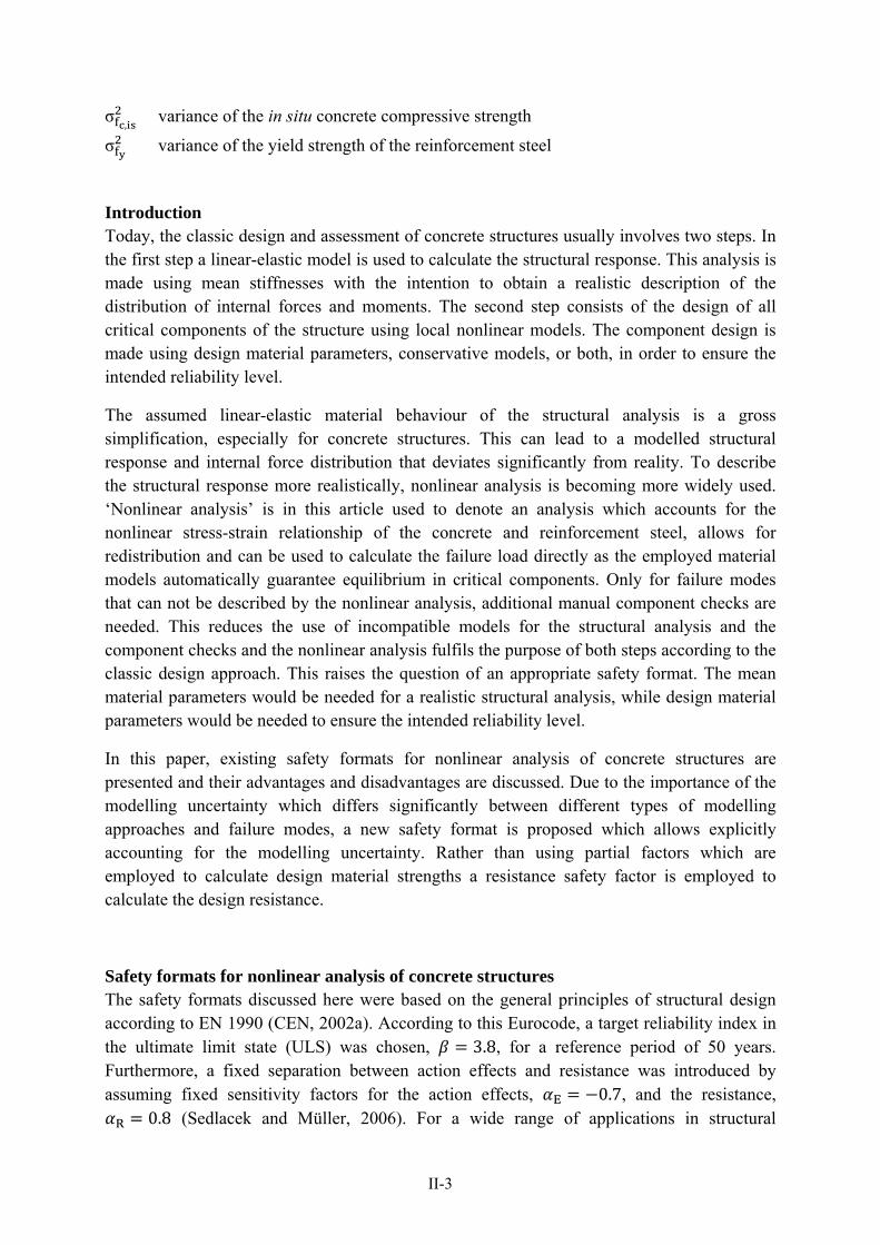
II-3
σ,
variance of the in situ concrete compressive strength
σ variance of the yield strength of the reinforcement steel
Introduction Today, the classic design and assessment of concrete structures usually involves two steps. In the first step a linear-elastic model is used to calculate the structural response. This analysis is made using mean stiffnesses with the intention to obtain a realistic description of the distribution of internal forces and moments. The second step consists of the design of all critical components of the structure using local nonlinear models. The component design is made using design material parameters, conservative models, or both, in order to ensure the intended reliability level.
The assumed linear-elastic material behaviour of the structural analysis is a gross simplification, especially for concrete structures. This can lead to a modelled structural response and internal force distribution that deviates significantly from reality. To describe the structural response more realistically, nonlinear analysis is becoming more widely used. ‘Nonlinear analysis’ is in this article used to denote an analysis which accounts for the nonlinear stress-strain relationship of the concrete and reinforcement steel, allows for redistribution and can be used to calculate the failure load directly as the employed material models automatically guarantee equilibrium in critical components. Only for failure modes that can not be described by the nonlinear analysis, additional manual component checks are needed. This reduces the use of incompatible models for the structural analysis and the component checks and the nonlinear analysis fulfils the purpose of both steps according to the classic design approach. This raises the question of an appropriate safety format. The mean material parameters would be needed for a realistic structural analysis, while design material parameters would be needed to ensure the intended reliability level.
In this paper, existing safety formats for nonlinear analysis of concrete structures are presented and their advantages and disadvantages are discussed. Due to the importance of the modelling uncertainty which differs significantly between different types of modelling approaches and failure modes, a new safety format is proposed which allows explicitly accounting for the modelling uncertainty. Rather than using partial factors which are employed to calculate design material strengths a resistance safety factor is employed to calculate the design resistance.
Safety formats for nonlinear analysis of concrete structures The safety formats discussed here were based on the general principles of structural design according to EN 1990 (CEN, 2002a). According to this Eurocode, a target reliability index in the ultimate limit state (ULS) was chosen, 3.8, for a reference period of 50 years. Furthermore, a fixed separation between action effects and resistance was introduced by assuming fixed sensitivity factors for the action effects, E 0.7, and the resistance,
R 0.8 (Sedlacek and Müller, 2006). For a wide range of applications in structural
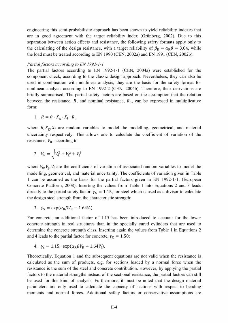
II-4
engineering this semi-probabilistic approach has been shown to yield reliability indexes that are in good agreement with the target reliability index (Grünberg, 2002). Due to this separation between action effects and resistance, the following safety formats apply only to the calculating of the design resistance, with a target reliability of R R 3.04, while the load must be treated according to EN 1990 (CEN, 2002a) and EN 1991 (CEN, 2002b).
Partial factors according to EN 1992-1-1 The partial factors according to EN 1992-1-1 (CEN, 2004a) were established for the component check, according to the classic design approach. Nevertheless, they can also be used in combination with nonlinear analysis; they are the basis for the safety format for nonlinear analysis according to EN 1992-2 (CEN, 2004b). Therefore, their derivations are briefly summarised. The partial safety factors are based on the assumption that the relation between the resistance, , and nominal resistance, , can be expressed in multiplicative form:
1.
where , , are random variables to model the modelling, geometrical, and material
uncertainty respectively. This allows one to calculate the coefficient of variation of the resistance, R, according to
2. R θ
where θ, , are the coefficients of variation of associated random variables to model the
modelling, geometrical, and material uncertainty. The coefficients of variation given in Table 1 can be assumed as the basis for the partial factors given in EN 1992-1-1, (European Concrete Platform, 2008). Inserting the values from Table 1 into Equations 2 and 3 leads directly to the partial safety factor, S 1.15, for steel which is used as a divisor to calculate the design steel strength from the characteristic strength:
3. S exp R R 1.64 .
For concrete, an additional factor of 1.15 has been introduced to account for the lower concrete strength in real structures than in the specially cured cylinders that are used to determine the concrete strength class. Inserting again the values from Table 1 in Equations 2 and 4 leads to the partial factor for concrete, C 1.50:
4. 1.15 exp R R 1.64 .
Theoretically, Equation 1 and the subsequent equations are not valid when the resistance is calculated as the sum of products, e.g. for sections loaded by a normal force when the resistance is the sum of the steel and concrete contribution. However, by applying the partial factors to the material strengths instead of the sectional resistance, the partial factors can still be used for this kind of analysis. Furthermore, it must be noted that the design material parameters are only used to calculate the capacity of sections with respect to bending moments and normal forces. Additional safety factors or conservative assumptions are
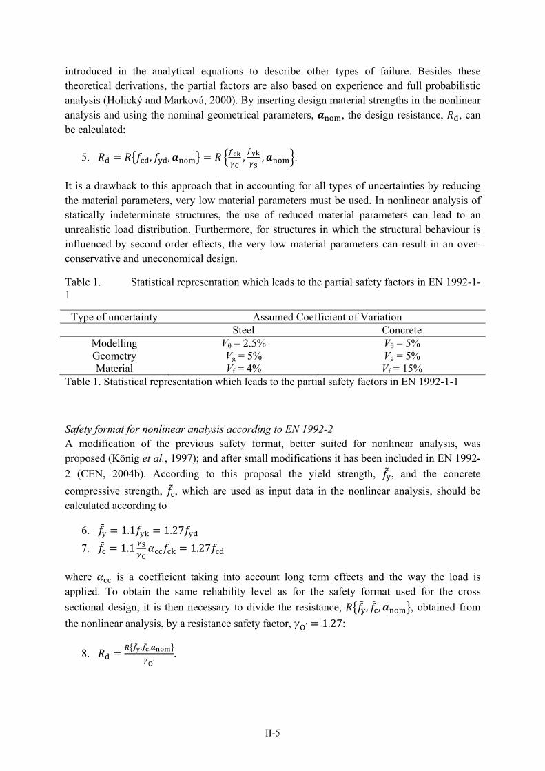
II-5
introduced in the analytical equations to describe other types of failure. Besides these theoretical derivations, the partial factors are also based on experience and full probabilistic analysis (Holický and Marková, 2000). By inserting design material strengths in the nonlinear analysis and using the nominal geometrical parameters, , the design resistance, , can be calculated:
5. , ,C
,S
, .
It is a drawback to this approach that in accounting for all types of uncertainties by reducing the material parameters, very low material parameters must be used. In nonlinear analysis of statically indeterminate structures, the use of reduced material parameters can lead to an unrealistic load distribution. Furthermore, for structures in which the structural behaviour is influenced by second order effects, the very low material parameters can result in an over-conservative and uneconomical design.
Table 1. Statistical representation which leads to the partial safety factors in EN 1992-1-1
Type of uncertainty Assumed Coefficient of Variation Steel Concrete
Modelling Vθ = 2.5% Vθ = 5% Geometry Vg = 5% Vg = 5% Material Vf = 4% Vf = 15%
Table 1. Statistical representation which leads to the partial safety factors in EN 1992-1-1
Safety format for nonlinear analysis according to EN 1992-2 A modification of the previous safety format, better suited for nonlinear analysis, was proposed (König et al., 1997); and after small modifications it has been included in EN 1992-
2 (CEN, 2004b). According to this proposal the yield strength, , and the concrete
compressive strength, , which are used as input data in the nonlinear analysis, should be calculated according to
6. 1.1 1.27
7. 1.1 S
C1.27
where is a coefficient taking into account long term effects and the way the load is applied. To obtain the same reliability level as for the safety format used for the cross
sectional design, it is then necessary to divide the resistance, , , , obtained from
the nonlinear analysis, by a resistance safety factor, O′ 1.27:
8. , ,
O′.
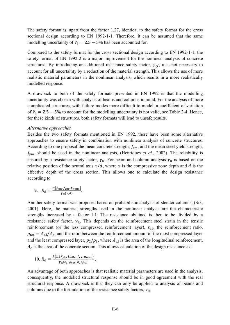
II-6
The safety format is, apart from the factor 1.27, identical to the safety format for the cross sectional design according to EN 1992-1-1. Therefore, it can be assumed that the same modelling uncertainty of θ 2.5 5% has been accounted for.
Compared to the safety format for the cross sectional design according to EN 1992-1-1, the safety format of EN 1992-2 is a major improvement for the nonlinear analysis of concrete structures. By introducing an additional resistance safety factor, O′, it is not necessary to
account for all uncertainty by a reduction of the material strength. This allows the use of more realistic material parameters in the nonlinear analysis, which results in a more realistically modelled response.
A drawback to both of the safety formats presented in EN 1992 is that the modelling uncertainty was chosen with analysis of beams and columns in mind. For the analysis of more complicated structures, with failure modes more difficult to model, a coefficient of variation of θ 2.5 5% to account for the modelling uncertainty is not valid, see Table 2-4. Hence, for these kinds of structures, both safety formats will lead to unsafe results.
Alternative approaches Besides the two safety formats mentioned in EN 1992, there have been some alternative approaches to ensure safety in combination with nonlinear analysis of concrete structures. According to one proposal the mean concrete strength, , and the mean steel yield strength,
, should be used in the nonlinear analysis, (Henriques et al., 2002). The reliability is
ensured by a resistance safety factor, R. For beam and column analysis R is based on the relative position of the neutral axis / , where is the compressive zone depth and is the effective depth of the cross section. This allows one to calculate the design resistance according to
9. , ,
R ,.
Another safety format was proposed based on probabilistic analysis of slender columns, (Six, 2001). Here, the material strengths used in the nonlinear analysis are the characteristic strengths increased by a factor 1.1. The resistance obtained is then to be divided by a resistance safety factor, R. This depends on the reinforcement steel strain in the tensile reinforcement (or the less compressed reinforcement layer), , the reinforcement ratio,
, ⁄ , and the ratio between the reinforcement amount of the most compressed layer
and the least compressed layer, / , where , is the area of the longitudinal reinforcement,
is the area of the concrete section. This allows calculation of the design resistance as:
10. . , . ,
R , , / .
An advantage of both approaches is that realistic material parameters are used in the analysis; consequently, the modelled structural response should be in good agreement with the real structural response. A drawback is that they can only be applied to analysis of beams and columns due to the formulation of the resistance safety factors, R.
II-7
A general safety format for nonlinear analysis All of the previously described safety formats are only applicable to nonlinear analysis of beams and columns. This is due either to the assumed modelling uncertainty, which is not appropriate for failure modes that are more difficult to model, or due to the criteria for calculating the resistance safety factor, which are not applicable to other types of analysis. To allow nonlinear analysis to be used for all types of reinforced concrete structures a new safety format is proposed in the following:
To yield a realistic image of reality, the mean concrete in situ material strength, , , the
mean yield strength of steel, , , and nominal values, , for the geometrical
parameters should be used in the analysis to calculate the resistance:
11. , , , .
The design resistance, , is obtained by division of the resistance, , by a resistance safety factor, R, which depends on the coefficient of variation of the resistance, R:
12. , , ,
R R .
Justified by the central limit theorem for products, and in line with EN 1992-1-1 (CEN, 2004a), it is assumed that the resistance is approximately log-normal distributed, which allows approximating the resistance safety factor as:
13. R exp R R
Following the principles of the safety format from EN 1992-1-1, the coefficient of variation of the resistance, R, should be calculated according to Equation 2 to account for the modelling, geometrical, and material uncertainty using, θ, and . A biased modelling approach can be
accounted for by computing the resistance safety factor as
14. RR R
where is the mean ratio of experimental strength over calculated strength for the chosen modelling approach. The safety format is summarised in Figure 1 and details to quantify the modelling, geometrical, and material uncertainty are given in the following sections.

II-8
Figure 1. Flow chart for new safety format
Modelling uncertainty While the variability of the resistance due to material uncertainty and geometrical uncertainty is explicitly accounted for, all other variability must be accounted for by the modelling uncertainty.
Uni-axial bending
For bending failure, the failure load obtained by nonlinear analysis usually agrees very well with the failure load that is obtained with hand calculations according to codes. Both calculation methods are usually based on the Euler-Bernoulli Hypothesis with a material response under uni-axial loading. Hence, for both procedures a similar modelling uncertainties can be assumed. For the classic design approach, the JCSS Model Code (JCSS, 2001) recommends mean ratio of 1.2 and a coefficient of variation of θ 15% for the component analysis. In Sustainable Bridges (Casas et al., 2007) the coefficient of variation
θ 6% is assumed.
To quantify the modelling uncertainty of nonlinear analysis, a round robin test of over-reinforced beams under 4-point bending was conducted, (van Mier and Ulfkjaer, 2000). Apart from the concrete, steel and geometrical properties, stress-strain diagrams for the concrete test with high-and low-friction-loading plates were specified in the invitation to the round robin test. Four beam types were tested: one small beam with normal strength concrete (NSC small), one large beam with normal strength concrete (NSC large), one beam made of high
II-9
strength concrete (HSC) and one beam of fibre reinforced high strength concrete (FRHSC). Each beam type was tested three times. One contribution (Kang et al., 1998) was excluded from this study as a range of solutions was provided. The mean ratio, , and the coefficients of variation of the modelled strengths, θ, are summarised in Table 2.
Table 2. Modelling uncertainty of over-reinforced beams
Beam type θ NSC small 0.93 10% NSC large 0.94 11% HSC 1.02 25%
FRHSC 0.98 26%
It can be seen that for the normal strength concrete beams non conservative results were obtained, whereas the coefficients of variation of the calculated failure loads were around than 10 %. For the high strength concretes much larger coefficients of variation were obtained but hardly any bias.
Shear failure
To quantify the modelling uncertainty for shear type failures, a modelling competition on shear panels from 1985 is available (Collins et al., 1985). Four different shear panels have been tested which were deliberately chosen as difficult to model. Some contributions were based on hand calculations, but no correlation between the complexity of the models and the accuracy of the resulting prediction has been found (Collins et al., 1985). Therefore, all contributions were included leading to Table 3.
Panel A was heavily reinforced and loaded in pure shear. It failed due to sliding of the concrete without yielding of the reinforcement prior to failure. Panel B was nominally identical to Panel A but was loaded in combined bi-axial compression and shear. It failed brittle due to the sliding of the concrete. For Panel C a non-isotropic reinforcement layout has been chosen so that the reinforcement yielded in one direction before the panel failed gradually involving crushing and sliding of the concrete. Panel D was non-isotropic reinforced and was first loaded in shear and later in combined shear and compression. It failed due to the sliding of the concrete.
Table 3. Modelling uncertainty for shear panels
Panel name θ
Panel A 0.87 16% Panel B 1.05 35% Panel C 0.97 21% Panel D 0.73 39%
II-10
For panels which were subjected to pure shear loading (Panel A and Panel C) a smaller variability of the predicted failure loads were obtained than for panels which were subjected to a combination of compression and shear loading. The predicted failure loads for Panel A and Panel D were significantly higher than the experimental ones.
Bending and shear failure in slabs
A modelling competition on slabs included eight slabs of differing thicknesses and reinforcement layout that were tested to failure (Jaeger and Marti, 2009b, Jaeger and Marti, 2009a). Some of these tests resulted in bending failure with yielding of the reinforcement, while others, typically when the slab was not provided with shear reinforcement, resulted in shear failure. One of the eight modelling contributions was based on hand calculations and was therefore excluded here from further analysis of the modelling competition which led to Table 4.
Table 4. Modelling uncertainty for bending and shear failure
Slab name
Slab Thickness
[mm]
Direction of bending
reinforcement Shear
reinforcement θ
A-1 200 45 No 0.79 27% A-2 200 45 Yes 0.89 9% B-1 200 0 No 1.00 24% B-2 200 0 Yes 1.04 5% C-1 500 45 No 0.72 34% C-2 500 45 Yes 0.89 11% D-1 500 0 No 0.97 29% D-2 500 0 Yes 1.12 3%
For the slabs without shear reinforcement, coefficients of variation in the range of θ 2434% were obtained. The use of shear reinforcement made the slabs easier to model and resulted in coefficients of variation on the range of θ 3 11%. By trend, the slabs with a thickness of 200 mm could be better modelled than the slabs with a thickness of 500 mm. For slabs with the bending reinforcement not aligned in the principle moment direction, the models overestimated the experimental failure load; most drastically for slab C-1 by 39 % on average!
Other failure modes
The most relevant failure modes of concrete structures are uni-axial bending and shear type failure. For related failure modes such as biaxial bending or torsional failure, higher modelling uncertainties must be expected. For concrete structures primarily under compression, the modelling uncertainty of over-reinforced concrete beams can be appropriate. To quantify the modelling uncertainty of anchor bolts, shells, and concrete containment vessels special studies are available (Elfgren et al., 2001, Krauthammer and Swartz, 1999, Hessheimer et al., 2001).
II-11
Summary
Based on the available data, coefficients of variation in the range of θ 5 30% seem appropriate for beams in bending. Values in the lower part can be chosen for failures due to yielding of the reinforcement steel. Intermediate values should be chosen for over-reinforced concrete beams of normal concrete, while values in the higher part should be chosen for over-reinforced high strength beams. Not aligning the bending reinforcement in the direction of the principal moments can lead to an overestimation of the strength which must be accounted for by 0.9.
For shear type failure the modelling uncertainty can be expected to lie in the range of
θ 10 40%. Values at the lower end of the range can be used for structures which fail due to yielding of the reinforcement steel. For small structures with simple loading that fail due to crushing of the concrete, values in the middle of the range seem appropriate. For a combination of compressive loading and shear loading and for larger structures higher coefficients of variation must be chosen. Furthermore, shear analysis can lead to a significant overestimation of the experimental failure load which can require a value of 0.7 1.0.
Despite the studies analysed here, the data to quantify the modelling uncertainty of nonlinear analysis is scarce and might neither be representative nor conclusive. The modelling uncertainty will depend on the chosen modelling approach and software and can therefore only be quantifying in quite wide ranges which are of limited practical help. This is especially problematic as the modelling uncertainty will often be the factor that will govern the calculation of the resistance safety factor, R. Until more studies are available which allow quantifying the modelling uncertainty more accurately, the choice of the modelling uncertainty will often depend on engineering judgement and can be subjective. Nevertheless, it is the authors’ opinion that a deliberate and thoughtful choice of the modelling uncertainty is better than assuming a coefficient of variation of θ 2.5 5% for all kinds of nonlinear models, as is currently done in EN 1992-2.
Geometrical uncertainty The geometrical uncertainty of reinforced concrete structures is usually quite small and has therefore minor influence on the resistance (JCSS, 2001). In these instances a coefficient of variation of 5% can be assumed, analogous to the derivations of the partial factors
according to EN 1992-1-1. For special types of structures that are sensitive to geometrical imperfections, e.g. slender columns, this assumption is not valid. In these cases the geometrical imperfections can be explicitly included in the nonlinear model to study their effect on the structural response.
II-12
Material uncertainty For structures with a resistance, , , … , , that depends linearly on the material parameters, , , … , , the variance of the resistance due to the material uncertainty can be calculated as
15. R ∑ ∑ Cov ,
where ⁄ is the partial derivative with respect to material parameters , is the
variance of material parameter , and Cov , is the covariance matrix. As the partial
derivatives are not usually explicitly available for nonlinear analysis, they have to be replaced by numerically evaluated different quotients. This requires repeated, computationally demanding nonlinear analysis. For example, describing the stress-strain diagram of the reinforcement steel by Young’s modulus, the yield strength, ultimate strength and ultimate strain and, for the concrete, by the compressive strength, tensile strength, fracture energy, and the crack bandwidth, would require as many as nine nonlinear analyses. In most situations, it is usually accurate enough to consider only the concrete compressive strength, , and the yield strength of the reinforcement steel, , as random variables. These two variables can be
used as reference parameters to which all other material parameters are deterministically related. The concrete compressive strength and the yield strength of the reinforcement are uncorrelated, which allows one to omit the right part of Equation 15 to obtain
16. RΔ
Δ
Δ
Δ ,.
For nonlinear response surfaces Equation 16 can lead to inaccurate results, but the inaccuracy can be reduced by an appropriate choice of the linearization interval. For the safety evaluation it is necessary that the linear approximation of the response surface should be in good agreement with the real response surface between the mean point and the design point. The exact design point is not known a priori and its determination is computationally expensive. Nevertheless, an appropriate linearization interval can be chosen, which will usually provide sufficient accuracy.
In accordance with the semi-probabilistic approach, it can be assumed that the sensitivity factor of the resistance side is usually in the neighbourhood of R 0.8. According to the previous section, the material uncertainty is approximately equal to the modelling uncertainty, e.g. for under-reinforced beams in bending, 5%, 5%. By disregarding the geometrical uncertainty, the sensitivity factor for the material uncertainty, , can therefore be
predicted as approximately R √2⁄ . Hence, it is suggested here that a step size parameter
be used, R /√2 2.15, which allows one to calculate, for the log-normally distributed
material strengths, the step sizes as ∆ X X 1 exp X . The coefficient of variation
of the resistance due to the material uncertainty, , can then be approximated as

II-13
17. ∆ , ,
∆
, , ∆
∆ , .
Structures in which the concrete tensile strength, rather than the compressive strength, limits the resistance the compressive strength and the associated variance used in Equation 17 must be replaced by the tensile strength and its associated variance. Furthermore, for very rare structures for which a decrease of the material parameters results in an increased resistance, the linearization interval can be adjusted, i.e. rather than using a linearization between the mean values and decreased material strength, the response surface should be approximated between the mean values and increased material strengths. To favour structures that fail with a ductile failure mode, due to yielding of the reinforcement steel, rather than a brittle mode due, to crushing of concrete, it is further possbile to introduce different weight factors into Equation 17.
An alternative, computationally less expensive, approach to estimating has been suggested (Cervenka et al., 2007). Instead of using three nonlinear finite element analyses, two analyses are required: one with the mean strengths and, and one with the characteristic
strengths using and, . To allow a fair comparison between both approaches to estimate
it was here chosen to use the mean in situ strengths , and , and the characteristic in
situ strengths and , , exp 1.64,
to yield:
18. log, , ,
, , , .
To see how accurately the coefficients of variation can be estimated using the previously described equations, they were tested on a, deliberately chosen, nonlinear response surface which refers to the maximum moment resistance of the beam section shown in Figure 2. The maximum moment resistance, , was calculated by the layered approach using 15 layers, i.e. discretising the beam over the depth, calculating the corresponding strains and stresses for each discretisation, and integrating the stresses over the depth. For the reinforcement steel the idealised stress-strain diagram, including strain hardening with an ultimate strength of
1.08 and a corresponding strain of 5% was used according to EN 1992-1-1,
(CEN, 2004a). For concrete in compression the stress-strain relation for the design of cross sections was used, (CEN, 2004a).
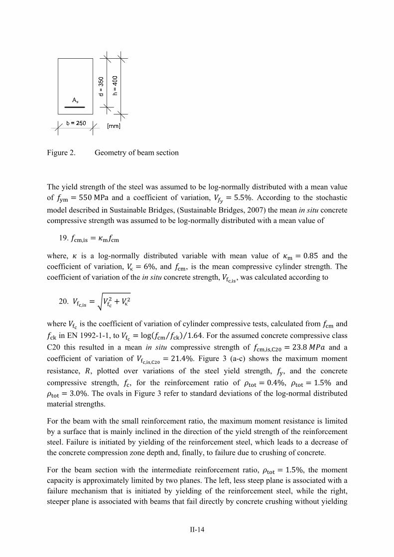
II-14
Figure 2. Geometry of beam section
The yield strength of the steel was assumed to be log-normally distributed with a mean value of 550 MPa and a coefficient of variation, 5.5%. According to the stochastic
model described in Sustainable Bridges, (Sustainable Bridges, 2007) the mean in situ concrete compressive strength was assumed to be log-normally distributed with a mean value of
19. ,
where, is a log-normally distributed variable with mean value of 0.85 and the coefficient of variation, κ 6%, and , is the mean compressive cylinder strength. The coefficient of variation of the in situ concrete strength,
,, was calculated according to
20. , κ
where is the coefficient of variation of cylinder compressive tests, calculated from and
in EN 1992-1-1, to log ⁄ 1.64⁄ . For the assumed concrete compressive class
C20 this resulted in a mean in situ compressive strength of , ,C 23.8 and a
coefficient of variation of , ,C
21.4%. Figure 3 (a-c) shows the maximum moment
resistance, , plotted over variations of the steel yield strength, , and the concrete
compressive strength, , for the reinforcement ratio of 0.4%, 1.5% and 3.0%. The ovals in Figure 3 refer to standard deviations of the log-normal distributed
material strengths.
For the beam with the small reinforcement ratio, the maximum moment resistance is limited by a surface that is mainly inclined in the direction of the yield strength of the reinforcement steel. Failure is initiated by yielding of the reinforcement steel, which leads to a decrease of the concrete compression zone depth and, finally, to failure due to crushing of concrete.
For the beam section with the intermediate reinforcement ratio, 1.5%, the moment capacity is approximately limited by two planes. The left, less steep plane is associated with a failure mechanism that is initiated by yielding of the reinforcement steel, while the right, steeper plane is associated with beams that fail directly by concrete crushing without yielding

II-15
of the reinforcement steel. When analysing the beam with mean strengths, the beam failure is initiated by yielding of the reinforcement steel. However, when looking at low failure probabilities that are relevant for the structural design, the beam will fail directly in compression of the concrete without yielding of the reinforcement. Hence, a single analysis using the mean material parameters can lead to misleading results concerning the material parameter that causes failure.
For the beam with the high reinforcement ratio, 3.0%, the concrete compressive strength limits the moment capacity for almost all combinations of material strengths, and failure occurs without yielding of the reinforcement steel. Consequently, the yield strength has almost no influence on the maximum moment resistance.
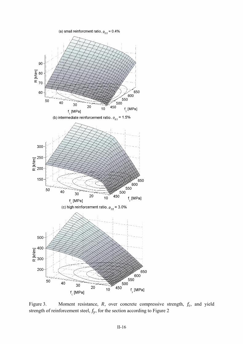
II-16
Figure 3. Moment resistance, , over concrete compressive strength, , and yield strength of reinforcement steel, , for the section according to Figure 2

II-17
For the beam section shown in Figure 2, Equations 17 and 18 were applied to calculate the coefficients of variation, , for seven reinforcement ratios, , and five step size parameters, c, see Table 5. The coefficients of variation increase for an increasing reinforcement ratio. For small reinforcement ratios the coefficients of variation are similar to the yield strength variation, 5.5%; for high reinforcement ratios, it approaches the coefficient of variation
of the concrete compressive strength, , ,C
21.4%.
The step size parameter has minor influence for the beams with either the low reinforcement ratios or the high reinforcement ratios. However, for the intermediate reinforcement ratios,
1.00 1.50%, which cause a change in failure mode, the estimated coefficients of variation differs by a factor of up to 2.3 between the smallest step size and the largest. This highlights the importance of an appropriate step size in the case of a nonlinear response surface.
Table 5. Coefficients of variation, , [%] according to Equations 17 and 18
Step size parameter reinforcement ratio, ρtot = As/Ac
c 0.40% 0.80% 1.00% 1.25% 1.50% 1.75% 3.00% Equation
17 0.50 5.3 5.7 6.1 6.8 7.6 17.6 18.2 1.64 5.5 6.3 6.9 8.7 14.2 18.2 18.8 2.15 5.7 6.6 7.3 11.2 15.4 18.5 19.0 3.08 5.9 7.3 9.8 13.9 16.8 18.9 19.3 3.80 6.1 8.5 12.1 15.4 17.6 19.3 19.6
Equation 18 0.50 7.8 8.8 9.3 10.4 11.4 20.6 21.8
1.64 7.3 8.3 9.0 9.9 13.4 18.3 19.5 2.15 7.2 8.4 9.0 10.0 14.3 18.2 19.3 3.08 7.3 8.5 9.3 11.8 15.4 18.2 19.3 3.80 7.3 8.7 9.5 13.0 15.9 18.2 19.3
To evaluate the consequences of the varying coefficients of variation, , on the safety analysis, this problem was first isolated for study, i.e. only the compressive strength and the yield strength of the reinforcement steel were assumed to be random variables, while all other parameters were assumed to be deterministically known.
The coefficients of variation, , in Table 5 were used to calculate the design resistance, ⁄ with exp , and an assumed target reliability index of 2.15. In the
next step Monte-Carlo simulations were used to calculate the probability, , and the
corresponding reliability index, Φ , where Φ is the standard normal
distribution function. The concrete compressive strength and the yield strength of the reinforcement steel were sampled from log-normal distributions. For each reinforcement ratio, a sample size of n = 106 was used. The reliability indexes obtained for the coefficients of variation according to Equations 17 and 18 and different step sizes are shown in Figure 4.
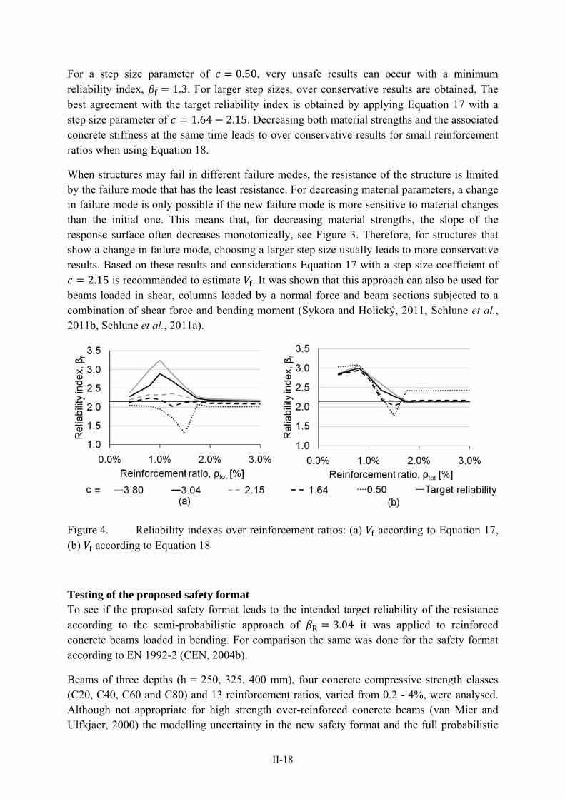
II-18
For a step size parameter of 0.50, very unsafe results can occur with a minimum reliability index, 1.3. For larger step sizes, over conservative results are obtained. The best agreement with the target reliability index is obtained by applying Equation 17 with a step size parameter of 1.64 2.15. Decreasing both material strengths and the associated concrete stiffness at the same time leads to over conservative results for small reinforcement ratios when using Equation 18.
When structures may fail in different failure modes, the resistance of the structure is limited by the failure mode that has the least resistance. For decreasing material parameters, a change in failure mode is only possible if the new failure mode is more sensitive to material changes than the initial one. This means that, for decreasing material strengths, the slope of the response surface often decreases monotonically, see Figure 3. Therefore, for structures that show a change in failure mode, choosing a larger step size usually leads to more conservative results. Based on these results and considerations Equation 17 with a step size coefficient of
2.15 is recommended to estimate . It was shown that this approach can also be used for beams loaded in shear, columns loaded by a normal force and beam sections subjected to a combination of shear force and bending moment (Sykora and Holický, 2011, Schlune et al., 2011b, Schlune et al., 2011a).
Figure 4. Reliability indexes over reinforcement ratios: (a) according to Equation 17, (b) according to Equation 18
Testing of the proposed safety format To see if the proposed safety format leads to the intended target reliability of the resistance according to the semi-probabilistic approach of R 3.04 it was applied to reinforced concrete beams loaded in bending. For comparison the same was done for the safety format according to EN 1992-2 (CEN, 2004b).
Beams of three depths (h = 250, 325, 400 mm), four concrete compressive strength classes (C20, C40, C60 and C80) and 13 reinforcement ratios, varied from 0.2 - 4%, were analysed. Although not appropriate for high strength over-reinforced concrete beams (van Mier and Ulfkjaer, 2000) the modelling uncertainty in the new safety format and the full probabilistic
II-19
analysis set at θ 5%. This choice was made to allow a better comparison between the safety formats and to avoid a bias in the comparison by different underlying assumptions. The geometrical uncertainty was assumed to be 5% and the coefficient of variation of the
material strength was estimated using Equation 17 with 2.15.
After calculating the design resistance according to the two safety formats, Monte-Carlo simulations were used to estimate the probability that the calculated resistances are below the design resistances, , using the limit state function
21. · , ,
where is a variable to model the modelling uncertainty. The stochastic model and the definition of the variables are given in Table 6. A sample size of n = 106 was used for each beam configuration.
Table 6. Stochastic model of basic variables
Symbol Dimension Distribution Mean
value, xm
Standard deviation,
σX
Materials Concrete, C20 fc,C20 MPa LN 23.8 0.214μX
Concrete, C40 fc,C40 MPa LN 40.8 0.126μX
Concrete, C60 fc,C60 MPa LN 57.8 0.097μX
Concrete, C80 fc,C80 MPa LN 74.8 0.084μX
Reinforcing Steel fy MPa LN 550 30 Geometrical data Effective depth d1 mm N 200 10
Effective depth d2 mm N 275 10
Effective depth d3 mm N 350 10 Modelling uncertainty – LN 1.00 0.05
Distribution types: N: normal, LN: log-normal
For the failure probabilities obtained the corresponding reliability indexes were calculated.
This yielded a mean reliability index of R,EN 2.95 with the coefficient of variation,
βR,EN9.5%, for the design according to EN 1992-2. For the new safety format, a mean
reliability index of R, 3.08 with the coefficient of variation βR,7.6% was
obtained. The histograms in Figure 5 confirm that the new safety format provides a reliability level that is closer to the target reliability and more constant than the current approach in EN 1992-2.
II-20
Figure 5. Reliability indices for sample structures
Discussion According to the classic design approach, boundary conditions and other uncertain structural parameters are often assumed “on the safe side”. However, for nonlinear analysis this approach leads to similar problems as using design material parameters, i.e. it cannot lead to a realistically modelled structural response. A possible remedy can be an extension of the approach adopted here to quantify the material uncertainty using a sensitivty study similar to the Gauss-approximation formula. To be better applicable to nonlinear problems, the response surface should not be linearised around the mean value using finite differences, but between the mean values and approximated design values.
Using the classic design approach, i.e. linear elastic analysis (without redistribution) followed by a check or design, of the critical section, to assure the safety on the component level, means that the load carrying capacity of the structure is limited by its most critical component. In contrast, nonlinear analysis reveals the maximum capacity of the entire modelled part. Depending on the extent of the modelled part, this can either correspond to the resistance of a single component or to the resistance of a complex structure with several possible failure modes. In addition, nonlinear analysis automatically redistributes stresses from softening elements to neighboring elements. Failure occures when no further redistribution is possbile. Hence, for nonlinear analysis, system reliability can play an important role, which has not been included in this study. The spatial variabily of the material parameters has not been included either.
Conclusions The safety format for nonlinear analysis of reinforced concrete structures, according to EN 1992-2 (CEN, 2004b), accounts for a coefficient of variation of the modelling uncertainty of 2.5-5% and does not account for possibly biased results. However, round robin tests and modelling competitions show that coefficients of variation of the modelled resistances lie typically in the range of 5 - 30% and for some structures a systematic overestimation of the strength was found. Hence, in many cases the safety format according to EN 1992-2 (CEN, 2004b) will not lead to the intended reliability level.
II-21
Based on the observation that the modelling uncertainty will often be the main factor that will govern the safety evaluation, a new safety format has been proposed which allows one to explicitly account for the modelling uncertainty. To avoid any interaction of the modelled response with the safety format, mean in situ material parameters should be used in the nonlinear analysis and a, so called, resistance safety factor is used to assure the intended reliability level. The material uncertainty can be estimated based on a sensitivity study that involves two additional nonlinear analyses, one with decreased steel parameters and the other with decreased concrete parameters.
Testing of the safety format on beam sections loaded in bending showed that it results in reliability indices that are in good agreement with the target reliability. Due to the assumption of a small modelling uncertainty only marginal improvements compared to the safety format according to EN 1992-2 could be shown. However, for nonlinear analysis of more difficult to model failure modes which result in a higher modelling uncertainty mayor improvements can be expected.
Due to the importance of the modelling uncertainty and the lack of data to quantify it, more round robin tests and modelling competitions are needed.
Acknowledgements The authors would like to express their gratitude to Sven Thelandersson, Professor at Lund University and Thomas Svensson, Ph.D., from the SP Technical Research Institute of Sweden for their help. Furthermore, The Swedish Research Council, FORMAS, and the Swedish Transport Administration, Trafikverket, are gratefully acknowledged for their financial support.
References CASAS, J. R., WISNIEWSKI, D. F., CERVENKA, J., CERVENKA, V., PUKL, R., BRUWHILER,
E., HERWIG, A., HOLM, G., OLSSON, M., BENGTSSON, P. E. & PLOS, M. (2007) Safety and Probabilistic Modelling: Background document D4.4. Sustainable Bridges.
CEN (2002a) EN 1990, Eurocode – Basis of structural design. Brussels, CEN, European Committee for Standardization.
CEN (2002b) EN 1991, Eurocode 1: Actions on structures. Brussels, CEN, European Committee for Standardization.
CEN (2004a) EN 1992-1-1, Eurocode 2: Design of concrete structures - Part 1-1: General rules and rules for buildings. Brussels, CEN, European Committee for Standardization.
CEN (2004b) EN 1992-2, Eurocode 2: Design of concrete structures - Part 2: Concrete bridges Design and detailing rules. Brussels, CEN European Committee for Standardization.
CERVENKA, V., CERVENKA, J. & PUKL, R. (2007) Safety assessment in fracture analysis of concrete structures. Proceedings of the 6th International Conference on Fracture Mechanics of Concrete and Concrete Structures. Catania, Italy .
COLLINS, M. P., VECCHIO, F. J. & MEHLHORN, G. (1985) An international competition to predict the response of reinforced concrete panels. Canadian Journal of Civil Engineering, 12: 624–644.

II-22
ELFGREN, L., ELIGEHAUSEN, R. & ROTS, J. (2001) Round Robin Analyses and Tests of Anchor Bolts in Concrete Structures. RILEM Technical Committee 90-FMA, Fracture Mechanics of Concrete - Applications. Luleå.
EUROPEAN CONCRETE PLATFORM ASBL, (2008) Eurocode 2 Commentary, Brussels, GRÜNBERG, J. (2002) Comments on EN 1990 "Basis of Structural Design", Berlin, Beuth Verlag. HENRIQUES, A. A. R., CALHEIROS, F. & FIGUEIRAS, J. A. (2002) Safety format for the design
of concrete frames. Engineering Computations, 19: 346–363. HESSHEIMER, M. F., LUK, V. K., KLAMERUS, E. W., SHIBATA, S., MITSUGI, S. &
COSTELLO, J. F. (2001) Pretest Round Robin Analysis of 1: 4-Scale Prestressed Concrete Containment Vessel Model. 9th International Conference on Nuclear Engineering. Nice, France.
HOLICKÝ, M. & MARKOVÁ, J. (2000) Verification of load factors for concrete components by reliability and optimization analysis: Background documents for implementing Eurocodes. Structural Control and Health Monitoring, 2: 502–507.
JAEGER, T. & MARTI, P. (2009a) Reinforced Concrete Slab Shear Prediction Competition: Entries and Discussion. ACI Structural Journal, 106.
JAEGER, T. & MARTI, P. (2009b) Reinforced Concrete Slab Shear Prediction Competition: Experiments. ACI Structural Journal, 106.
JCSS (2001) Probabilistic Model Code. Zurich, Joint Committee on Structural Safety, 12th Draft. KANG, H. D., SPACONE, E. & WILLAM, K. J. (1998) A study of compressive failure in over-
reinforced concrete beams. Third International Conference on Fracture Mechanics of Concrete and Concrete Structures. Gifu, Japan.
KÖNIG, G., NGUYEN, T. & AHNER, C. (1997) Consistent safety format. Non-linear Analysis: Discussion Papers from the Working Party in Commission 1. Lausanne, Comité Euro-International du Béton (CEB), Bulletin d' Information 239.
KRAUTHAMMER, T. & SWARTZ, S. E. (1999) Observed finite element capabilities and limitations from multi-team simulations of three concrete shell structures. Computers and Structures, 71: 277–291.
SCHLUNE, H., PLOS, M. & GYLLTOFT, K. (2011a) Comparative Study of Safety Formats for Nonlinear Finite Element Analysis of Concrete Structures. 11th International Conference on Applications of Statistics and Probability in Civil Engineering. Zurich, Switzerland.
SCHLUNE, H., PLOS, M. & GYLLTOFT, K. (2011b) Testing of Safety Formats for Nonlinear Analysis on Concrete Beams Subjected to Shear Forces and Bending Moments. revised version submitted to Engineering Structures, March 2011.
SEDLACEK, G. & MÜLLER, C. (2006) The European standard family and its basis. Journal of Constructional Steel Research, 62: 1047–1059.
SIX, M. (2001) Sicherheitskonzept für nichtlinear Traglastverfahren im Betonbau. Institut für Massivbau. PhD thesis, Technical University Darmstadt.
SUSTAINABLE BRIDGES (2007) Guideline for Load and Resistance Assessment of Existing European Railway Bridges: Advices on the use of advanced methods.
SYKORA, M. & HOLICKÝ, M. (2011) Safety Format for Non-linear Analysis in the Model Code - Verification of Reliability Level. fib Symposium: "Concrete engineering for excellence and efficiency". Prague, Czech Republic.
VAN MIER, J. G. M. & ULFKJAER, J. P. (2000) Round-Robin analysis of over-reinforced concrete beams – Comparison of results. Materials and Structures, 33: 381–390.
Paper III
Testing of Safety Formats for Nonlinear Analysis on Concrete Beams Subjected to Shear Forces and Bending Moments.
Accepted for publication in Engineering Structures, April 2011.

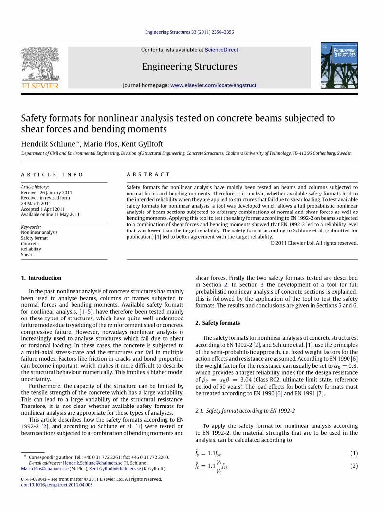
Engineering Structures 33 (2011) 2350–2356
Contents lists available at ScienceDirect
Engineering Structures
journal homepage: www.elsevier.com/locate/engstruct
Safety formats for nonlinear analysis tested on concrete beams subjected toshear forces and bending momentsHendrik Schlune ∗, Mario Plos, Kent GylltoftDepartment of Civil and Environmental Engineering, Division of Structural Engineering, Concrete Structures, Chalmers University of Technology, SE-412 96 Gothenburg, Sweden
a r t i c l e i n f o
Article history:Received 26 January 2011Received in revised form29 March 2011Accepted 1 April 2011Available online 11 May 2011
Keywords:Nonlinear analysisSafety formatConcreteReliabilityShear
a b s t r a c t
Safety formats for nonlinear analysis have mainly been tested on beams and columns subjected tonormal forces and bending moments. Therefore, it is unclear, whether available safety formats lead tothe intended reliability when they are applied to structures that fail due to shear loading. To test availablesafety formats for nonlinear analysis, a tool was developed which allows a full probabilistic nonlinearanalysis of beam sections subjected to arbitrary combinations of normal and shear forces as well asbendingmoments. Applying this tool to test the safety format according to EN 1992-2 on beams subjectedto a combination of shear forces and bending moments showed that EN 1992-2 led to a reliability levelthat was lower than the target reliability. The safety format according to Schlune et al. (submitted forpublication) [1] led to better agreement with the target reliability.
© 2011 Elsevier Ltd. All rights reserved.
1. Introduction
In the past, nonlinear analysis of concrete structures hasmainlybeen used to analyse beams, columns or frames subjected tonormal forces and bending moments. Available safety formatsfor nonlinear analysis, [1–5], have therefore been tested mainlyon these types of structures, which have quite well understoodfailuremodes due to yielding of the reinforcement steel or concretecompressive failure. However, nowadays nonlinear analysis isincreasingly used to analyse structures which fail due to shearor torsional loading. In these cases, the concrete is subjected toa multi-axial stress-state and the structures can fail in multiplefailure modes. Factors like friction in cracks and bond propertiescan become important, which makes it more difficult to describethe structural behaviour numerically. This implies a higher modeluncertainty.
Furthermore, the capacity of the structure can be limited bythe tensile strength of the concrete which has a large variability.This can lead to a large variability of the structural resistance.Therefore, it is not clear whether available safety formats fornonlinear analysis are appropriate for these types of analyses.
This article describes how the safety formats according to EN1992-2 [2], and according to Schlune et al. [1] were tested onbeamsections subjected to a combination of bendingmoments and
∗ Corresponding author. Tel.: +46 0 31 772 2261; fax: +46 0 31 772 2260.E-mail addresses: [email protected] (H. Schlune),
[email protected] (M. Plos), [email protected] (K. Gylltoft).
0141-0296/$ – see front matter© 2011 Elsevier Ltd. All rights reserved.doi:10.1016/j.engstruct.2011.04.008
shear forces. Firstly the two safety formats tested are describedin Section 2. In Section 3 the development of a tool for fullprobabilistic nonlinear analysis of concrete sections is explained;this is followed by the application of the tool to test the safetyformats. The results and conclusions are given in Sections 5 and 6.
2. Safety formats
The safety formats for nonlinear analysis of concrete structures,according to EN 1992-2 [2], and Schlune et al. [1], use the principlesof the semi-probabilistic approach, i.e. fixed weight factors for theaction effects and resistance are assumed. According to EN 1990 [6]the weight factor for the resistance can usually be set to αR = 0.8,which provides a target reliability index for the design resistanceof βR = αRβ = 3.04 (Class RC2, ultimate limit state, referenceperiod of 50 years). The load effects for both safety formats mustbe treated according to EN 1990 [6] and EN 1991 [7].
2.1. Safety format according to EN 1992-2
To apply the safety format for nonlinear analysis accordingto EN 1992-2, the material strengths that are to be used in theanalysis, can be calculated according to
fy = 1.1fyk (1)
fc = 1.1γs
γcfck (2)
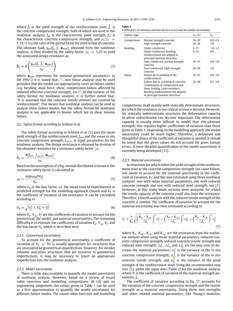
H. Schlune et al. / Engineering Structures 33 (2011) 2350–2356 2351
where fy is the yield strength of the reinforcement steel, fc isthe concrete compressive strength, both of which are used in thenonlinear analysis, fyk is the characteristic yield strength, fck isthe characteristic concrete compressive strength, and γs/γc =
1.15/1.5 is the ratio of the partial factor for steel to that of concrete.The ultimate load, qud{fy, fc, anom}, obtained from the nonlinearanalysis, is then divided by the safety factor, γO′ = 1.27 to yieldthe associated design resistance as:
Rd = R
qud{fy, fc, anom}
γO′
(3)
where anom represents the nominal geometrical parameters. InEN 1992-2 it is stated that: ‘‘. . .non linear analysis may be usedprovided that the model can appropriately cover all failure modes(e.g. bending, axial force, shear, compression failure affected byreduced effective concrete strength, etc.)’’. In the context of thesafety format for nonlinear analysis, it is further noted that:‘‘It is assumed that the concrete tensile stresses are covered byreinforcement’’. This means that nonlinear analysis can be used toanalyse shear failure modes, but the safety format for nonlinearanalysis is not applicable to beams which fail in shear tensionfailure.
2.2. Safety format according to Schlune et al.
The safety format according to Schlune et al. [1] uses the meanyield strength of the reinforcement steel, fym, and the mean in situconcrete compressive strength, fcm,is, as input parameters for thenonlinear analysis. The design resistance is obtained by division ofthe obtained resistance by a resistance safety factor, γR:
Rd =R{fym, f cm,is, anom}
γR. (4)
Based on the assumptionof a log-normal distributed resistance, theresistance safety factor is calculated as
γR =exp(αRβVR)
θm(5)
where θm is the bias factor, i.e. the mean ratio of experimental topredicted strength for the modelling approach chosen and VR isthe coefficient of variation of the resistance. It can be calculatedaccording to
VR =
V 2g + V 2
m + V 2f (6)
where Vg , Vm, Vf are the coefficients of variation to account for thegeometrical, the model, and material uncertainties. The remainingdifficulty is to estimate the coefficients of variation Vg , Vm, Vf , andthe bias factor θm which is described next.
2.2.1. Geometrical uncertaintyTo account for the geometrical uncertainty, a coefficient of
variation of Vg = 5% is usually appropriate for structures thatare insensitive to geometrical imperfections. However, for slendercolumns and other structures that are sensitive to geometricalimperfections, it may be necessary to insert an appropriateimperfection into the nonlinear analysis.
2.2.2. Model uncertaintyThere is little data available to quantify the model uncertainty
of nonlinear analysis. However, based on a review of roundrobin exercises and modelling competitions [8–14] and onengineering judgement, the values given in Table 1 can be usedas a first approximation to quantify the model uncertainty fordifferent failure modes. The round robin exercises and modelling
Table 1Coefficients of variation and bias factors to account for model uncertainty.
Failure type Vm (%) θm
Compression Normal strength concrete 10–20 0.9–1.0High strength concrete 20–30 1.0
Bending Under-reinforced 5–15 1.0–1.2Under-reinforced, bendingreinforcement not aligned inprincipal moment direction
5–15 0.9
Over-reinforced, normal strengthconcrete
10–15 0.9–1.0
Over-reinforced, high strengthconcrete
20–30 1.0
Shear Failure do to yielding of thereinforcement
10–25 0.9–1.0
Failure due to crushing of concrete,Combination of compression andshear loading, Large members,Bending reinforcement not alignedin principal moment direction
20–40 0.7–1.0
competitions dealt mainly with statically determinate structures,forwhich the resistance in one critical section is decisive. However,for statically indeterminate structures the deformation capacityto allow redistribution can become important. The deformationcapacity is usually more difficult to model than the ultimatestrength; this requires higher coefficients of variation than thosegiven in Table 1. Depending on the modelling approach, the modeluncertainty could be much higher. Therefore, a deliberate andthoughtful choice of the coefficient of variation is needed. It shouldbe noted that the given values do not account for gross humanerrors. A more detailed quantification of the model uncertainty iscurrently being developed [15].
2.2.3. Material uncertaintyIn structures forwhich either the yield strength of the reinforce-
ment steel or the concrete compressive strength can cause failure,one needs to account for the material uncertainty in the coeffi-cient of variation, Vf , and this was estimated using three nonlinearanalyses: one with mean material parameters, one with reducedconcrete strength and one with reduced steel strength, see [1].However, in this study beam sections were analysed, for whichthe tensile capacity of the concrete could also limit the resistance.Therefore, a fourth analysiswith the reduced tensile strength of theconcrete is needed. The coefficient of variation to account for thematerial uncertainty was then estimated according to
Vf ≈1Rm
Rm − R△fc
△fc
2
σ 2fc +
Rm − R△fct
△fct
2
σ 2fct +
Rm − R△fy
△fy
2
σ 2fy
(7)
where Rm, R△fc , R△fct and R△fy are the resistances from the nonlin-ear analysis when using mean material parameters, reduced con-crete compressive strength, reduced concrete tensile strength andreduced steel strength; △fc , △fct and △fy are the step sizes to de-crease the material parameters; σ 2
fc is the variance of the in situconcrete compressive strength; σ 2
fct is the variance of the in situconcrete tensile strength; and σ 2
fy is the variance of the yieldstrength of the reinforcement steel. Using the recommended stepsize, [1], yields the input data (Table 2) for the nonlinear analysiswhere Vi is the coefficient of variation of the material strength pa-rameter, fi.
The coefficient of variation according to Eq. (7) accounts forthe variation of the concrete compressive strength and the tensilestrength as a material uncertainty. Using these two strengthsand other related material parameters, like Young’s modulus,
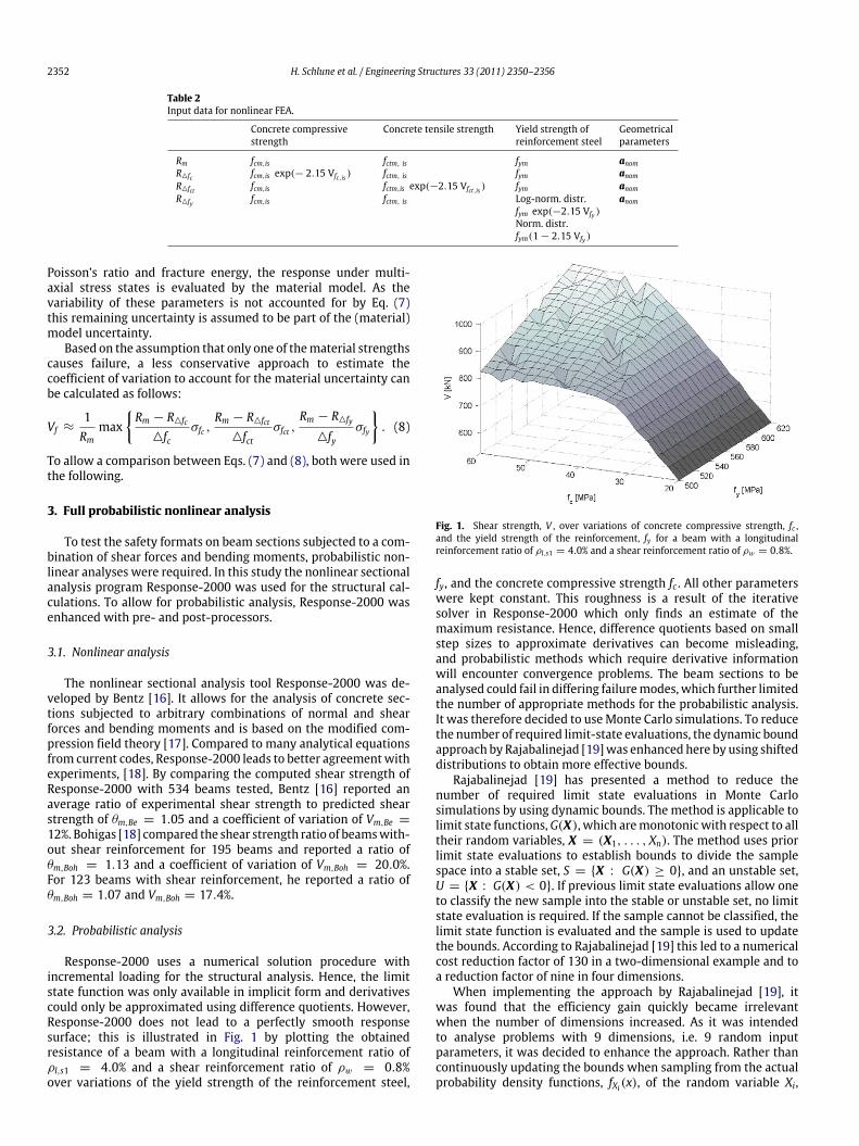
2352 H. Schlune et al. / Engineering Structures 33 (2011) 2350–2356
Table 2Input data for nonlinear FEA.
Concrete compressivestrength
Concrete tensile strength Yield strength ofreinforcement steel
Geometricalparameters
Rm fcm,is fctm, is fym anomR△fc fcm,is exp(− 2.15 Vfc,is ) fctm, is fym anomR△fct fcm,is fctm,is exp(−2.15 Vfct,is ) fym anomR△fy fcm,is fctm, is Log-norm. distr.
fym exp(−2.15 Vfy )
Norm. distr.fym(1 − 2.15 Vfy )
anom
Poisson’s ratio and fracture energy, the response under multi-axial stress states is evaluated by the material model. As thevariability of these parameters is not accounted for by Eq. (7)this remaining uncertainty is assumed to be part of the (material)model uncertainty.
Based on the assumption that only one of thematerial strengthscauses failure, a less conservative approach to estimate thecoefficient of variation to account for the material uncertainty canbe calculated as follows:
Vf ≈1Rm
maxRm − R△fc
△fcσfc ,
Rm − R△fct
△fctσfct ,
Rm − R△fy
△fyσfy
. (8)
To allow a comparison between Eqs. (7) and (8), both were used inthe following.
3. Full probabilistic nonlinear analysis
To test the safety formats on beam sections subjected to a com-bination of shear forces and bending moments, probabilistic non-linear analyses were required. In this study the nonlinear sectionalanalysis program Response-2000 was used for the structural cal-culations. To allow for probabilistic analysis, Response-2000 wasenhanced with pre- and post-processors.
3.1. Nonlinear analysis
The nonlinear sectional analysis tool Response-2000 was de-veloped by Bentz [16]. It allows for the analysis of concrete sec-tions subjected to arbitrary combinations of normal and shearforces and bending moments and is based on the modified com-pression field theory [17]. Compared to many analytical equationsfrom current codes, Response-2000 leads to better agreementwithexperiments, [18]. By comparing the computed shear strength ofResponse-2000 with 534 beams tested, Bentz [16] reported anaverage ratio of experimental shear strength to predicted shearstrength of θm,Be = 1.05 and a coefficient of variation of Vm,Be =
12%. Bohigas [18] compared the shear strength ratio of beamswith-out shear reinforcement for 195 beams and reported a ratio ofθm,Boh = 1.13 and a coefficient of variation of Vm,Boh = 20.0%.For 123 beams with shear reinforcement, he reported a ratio ofθm,Boh = 1.07 and Vm,Boh = 17.4%.
3.2. Probabilistic analysis
Response-2000 uses a numerical solution procedure withincremental loading for the structural analysis. Hence, the limitstate function was only available in implicit form and derivativescould only be approximated using difference quotients. However,Response-2000 does not lead to a perfectly smooth responsesurface; this is illustrated in Fig. 1 by plotting the obtainedresistance of a beam with a longitudinal reinforcement ratio ofρl,s1 = 4.0% and a shear reinforcement ratio of ρw = 0.8%over variations of the yield strength of the reinforcement steel,
Fig. 1. Shear strength, V , over variations of concrete compressive strength, fc ,and the yield strength of the reinforcement, fy for a beam with a longitudinalreinforcement ratio of ρl,s1 = 4.0% and a shear reinforcement ratio of ρw = 0.8%.
fy, and the concrete compressive strength fc . All other parameterswere kept constant. This roughness is a result of the iterativesolver in Response-2000 which only finds an estimate of themaximum resistance. Hence, difference quotients based on smallstep sizes to approximate derivatives can become misleading,and probabilistic methods which require derivative informationwill encounter convergence problems. The beam sections to beanalysed could fail in differing failuremodes, which further limitedthe number of appropriate methods for the probabilistic analysis.It was therefore decided to useMonte Carlo simulations. To reducethe number of required limit-state evaluations, the dynamic boundapproach by Rajabalinejad [19]was enhanced here by using shifteddistributions to obtain more effective bounds.
Rajabalinejad [19] has presented a method to reduce thenumber of required limit state evaluations in Monte Carlosimulations by using dynamic bounds. The method is applicable tolimit state functions,G(X), which aremonotonicwith respect to alltheir random variables, X = (X1, . . . , Xn). The method uses priorlimit state evaluations to establish bounds to divide the samplespace into a stable set, S = {X : G(X) ≥ 0}, and an unstable set,U = {X : G(X) < 0}. If previous limit state evaluations allow oneto classify the new sample into the stable or unstable set, no limitstate evaluation is required. If the sample cannot be classified, thelimit state function is evaluated and the sample is used to updatethe bounds. According to Rajabalinejad [19] this led to a numericalcost reduction factor of 130 in a two-dimensional example and toa reduction factor of nine in four dimensions.
When implementing the approach by Rajabalinejad [19], itwas found that the efficiency gain quickly became irrelevantwhen the number of dimensions increased. As it was intendedto analyse problems with 9 dimensions, i.e. 9 random inputparameters, it was decided to enhance the approach. Rather thancontinuously updating the bounds when sampling from the actualprobability density functions, fXi(x), of the random variable Xi,

H. Schlune et al. / Engineering Structures 33 (2011) 2350–2356 2353
a b
Fig. 2. Bounds according to Rajabalinejad [19] (a) and the approach used here (b).
some importance sampling density functions, hXi(x), were used toconstruct the bounds. A sample, x, of hXi(x) was generated by firstgenerating a sample, u, of the standard normal distribution. In thenext step the sample was shifted by a constant distance,1u, closerto the limit state, that is us = u + 1u for variables in which thelimit state function is monotonically decreasing and us = u − 1ufor variables in which the limit state function is increasing. Finally,the sample was calculated according to x = F−1
Xi(Φ(us)) where FXi
is the distribution function and Φ is the standardised distributionfunction. Furthermore, for small failure probabilities, which wereof interest in this study, hardly any computational benefits aregained by using bounds for the unstable set. Therefore, only thestable set was used here.
In Fig. 2 the Rajabalinejad approach to constructing thebounds [19] and the approach used here are illustrated by a two-dimensional problem in the standard normal space. Eleven andten samples, respectively, were used to construct the bounds. Thegrey areas mark the samples for which no limit state evaluationsare needed. It can be seen that the approach used here leads tomore efficient bounds. The extra computational effort to constructthe bounds from the importance sampling density, instead of theactual probability density, is usually quickly compensated.
4. Testing of the safety formats
4.1. Procedure
To test the safety formats, the flow chart shown in Fig. 3 wasapplied. First, the safety formats were used to calculate designresistances for the structures studied according to both testedsafety formats. To apply the safety format according to Schluneet al. [1] a coefficient of variation of Vg = 5% was assumed toaccount for the geometrical uncertainty and Eqs. (7) and (8) wereused to estimate Vf . The coefficients of variation, Vm,Be and Vm,Boh,and the bias factors, θm,Be and θm,Boh, to account for the modeluncertainty according to Section 3.1 were used.
Then 3000–4000 samples from the importance samplingdensity, h(x), were taken to construct the bounds. For the casesanalysed here the shifting distances were in the range of △u =
1.25–1.55 so that approximately 50% of the samples from h(x)were stable.
In a next step 300,000 samples were generated from f (x) toestimate the probability P(R < Rd) using the limit state function
G(X) = θiR(fc, fct , fy, fu, εu, b, h, cnom) − Rd (9)
Fig. 3. Flow chart for testing of the safety formats.
where fu is the ultimate strength of the reinforcement steel, εu isthe ultimate strain of the reinforcement steel, b is the width ofthe beam, h is the height of the beam and cnom is the concretecover at the bottom of the beam. The bounds were used to reducethe number of limit state evaluations. For the 9-dimensionalproblem, a computation cost reduction by a factor of 5–55 wasobtained. To assure that the bounds did not falsify the failureprobability, selected structures were analysed using bounds anda function evaluation for each sample. No difference in failureprobability was found despite the rough response surfaces. Finally,
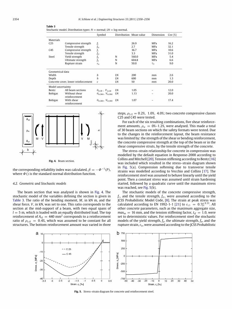
2354 H. Schlune et al. / Engineering Structures 33 (2011) 2350–2356
Table 3Stochastic model. Distribution types: N = normal; LN = log-normal.
Symbol Distribution Mean value Dimension Cov (%)
MaterialsC25 Compressive strength fc 26.9 MPa 16.2
Tensile strength fct 2.7 MPa 32.1C45 Compressive strength fc 36.7 MPa 10.6
Tensile strength fct 3.3 MPa 31.0Steel Yield strength fy N 560.0 MPa 5.4
Ultimate strength fu N 604.8 MPa 6.6Rupture strain εu N 50.0 h 9.0
Geometrical dataWidth b LN 200 mm 2.6Depth h LN 600 mm 1.3Concrete cover, lower reinforcement c LN 50 mm 20.0
Model uncertaintyBentz All beam sections θm,Be , Vm,Be LN 1.05 – 12.0Bohigas Without shear
reinforcementθm,Boh, Vm,Boh LN 1.13 – 20.0
Bohigas With shearreinforcement
θm,Boh, Vm,Boh LN 1.07 – 17.4
Fig. 4. Beam section.
the corresponding reliability index was calculated, β = −Φ−1(P),where Φ() is the standard normal distribution function.
4.2. Geometric and Stochastic models
The beam section that was analysed is shown in Fig. 4. Thestochastic model of the variables defining the section is given inTable 3. The ratio of the bending moment, M , in kN m, and theshear force, V , in kN, was set to one. This ratio corresponds to thesection at the mid-support of a beam, with two equal spans ofl = 5 m, which is loaded with an equally distributed load. The topreinforcement of As2 = 440 mm2 corresponds to a reinforcementratio of ρl,s2 = 0.4%, which was assumed to be constant for allstructures. The bottom reinforcement amount was varied in three
steps, ρl,s1 = 0.2%, 1.0%, 4.0%; two concrete compressive classesC25 and C45 were tested.
For each of the six resulting combinations, five shear reinforce-ment amounts, ρw = 0%–1.2%, were analysed. This made a totalof 30 beam sections on which the safety formats were tested. Dueto the changes in the reinforcement layout, the beam resistancewas limited by: the strength of the shear or bending reinforcement,the concrete compressive strength at the top of the beam or in theshear compressive struts, by the tensile strength of the concrete.
The stress–strain relationship for concrete in compression wasmodelled by the default equation in Response-2000 according toCollins andMitchell [20]. Tension stiffening according to Bentz [16]was included which resulted in the stress–strain diagram shownin Fig. 5(a). Compression softening due to transverse tensilestrains was modelled according to Vecchio and Collins [17]. Thereinforcement steel was assumed to behave linearly until the yieldpoint. Then a constant stress was assumed until strain hardeningstarted, followed by a quadratic curve until the maximum stresswas reached, see Fig. 5(b).
The stochastic models of the concrete compressive strength,fc , and the tensile strength, fct , were assumed according to theJCSS Probabilistic Model Code, [8]. The strain at peak stress wascalculated according to EN 1992-1-1 [21] to εc1 = 0.7fc0.31. Allother concrete parameters, such as the maximum aggregate size,maxas = 16 mm, and the tension stiffening factor, tsf = 1.0, wereset to deterministic values. For reinforcement steel the stochasticmodels of the yield strength, fy, the ultimate strength, fu, and therupture strain, εu, were assumed according to the JCSS Probabilistic
a b
Fig. 5. Stress–strain diagram for concrete and reinforcement steel.
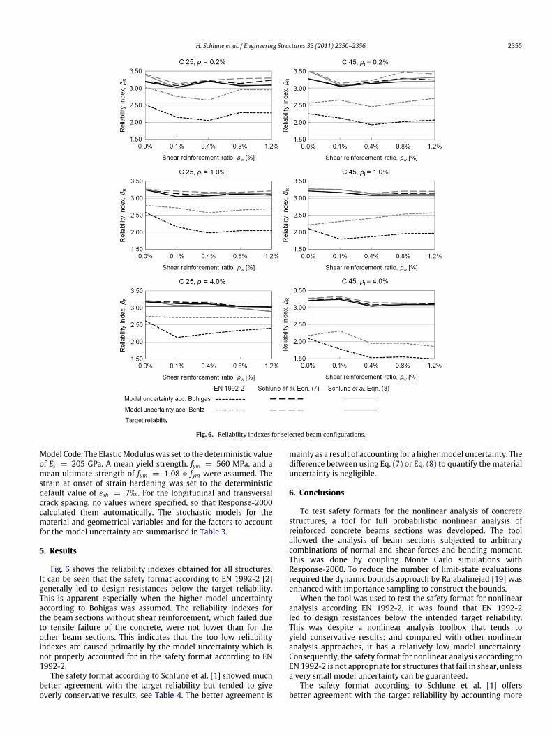
H. Schlune et al. / Engineering Structures 33 (2011) 2350–2356 2355
Fig. 6. Reliability indexes for selected beam configurations.
Model Code. The ElasticModuluswas set to the deterministic valueof Es = 205 GPa. A mean yield strength, fym = 560 MPa, and amean ultimate strength of fum = 1.08 ∗ fym were assumed. Thestrain at onset of strain hardening was set to the deterministicdefault value of εsh = 7h. For the longitudinal and transversalcrack spacing, no values where specified, so that Response-2000calculated them automatically. The stochastic models for thematerial and geometrical variables and for the factors to accountfor the model uncertainty are summarised in Table 3.
5. Results
Fig. 6 shows the reliability indexes obtained for all structures.It can be seen that the safety format according to EN 1992-2 [2]generally led to design resistances below the target reliability.This is apparent especially when the higher model uncertaintyaccording to Bohigas was assumed. The reliability indexes forthe beam sections without shear reinforcement, which failed dueto tensile failure of the concrete, were not lower than for theother beam sections. This indicates that the too low reliabilityindexes are caused primarily by the model uncertainty which isnot properly accounted for in the safety format according to EN1992-2.
The safety format according to Schlune et al. [1] showed muchbetter agreement with the target reliability but tended to giveoverly conservative results, see Table 4. The better agreement is
mainly as a result of accounting for a highermodel uncertainty. Thedifference between using Eq. (7) or Eq. (8) to quantify the materialuncertainty is negligible.
6. Conclusions
To test safety formats for the nonlinear analysis of concretestructures, a tool for full probabilistic nonlinear analysis ofreinforced concrete beams sections was developed. The toolallowed the analysis of beam sections subjected to arbitrarycombinations of normal and shear forces and bending moment.This was done by coupling Monte Carlo simulations withResponse-2000. To reduce the number of limit-state evaluationsrequired the dynamic bounds approach by Rajabalinejad [19] wasenhanced with importance sampling to construct the bounds.
When the tool was used to test the safety format for nonlinearanalysis according EN 1992-2, it was found that EN 1992-2led to design resistances below the intended target reliability.This was despite a nonlinear analysis toolbox that tends toyield conservative results; and compared with other nonlinearanalysis approaches, it has a relatively low model uncertainty.Consequently, the safety format for nonlinear analysis according toEN 1992-2 is not appropriate for structures that fail in shear, unlessa very small model uncertainty can be guaranteed.
The safety format according to Schlune et al. [1] offersbetter agreement with the target reliability by accounting more
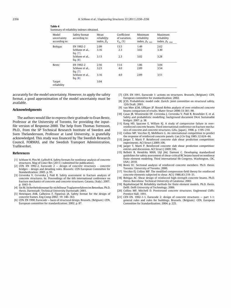
2356 H. Schlune et al. / Engineering Structures 33 (2011) 2350–2356
Table 4Summary of reliability indexes obtained.
Modeluncertaintyaccording to:
Safety formataccording to:
Meanreliabilityindex, βR
Coefficientof variation,VβR (%)
Minimumreliabilityindex, βR, min
Maximumreliabilityindex, βR, max
Bohigas EN 1992-2 2.09 13.5 1.49 2.62Schlune et al.,Eq. (7)
3.16 2.3 3.02 3.30
Schlune et al.,Eq. (8)
3.13 2.3 3.02 3.28
Bentz EN 1992-2 2.56 11.6 1.86 3.04Schlune et al.,Eq. (7)
3.23 4.0 2.89 3.54
Schlune et al.,Eq. (8)
3.16 4.0 2.89 3.51
Targetreliability
3.04
accurately for the model uncertainty. However, to apply the safetyformat, a good approximation of the model uncertainty must beavailable.
Acknowledgments
The authors would like to express their gratitude to Evan Bentz,Professor at the University of Toronto, for providing the input-file version of Response-2000. The help from Thomas Svensson,Ph.D., from the SP Technical Research Institute of Sweden andSven Thelandersson, Professor at Lund University, is gratefullyacknowledged. This study was financed by The Swedish ResearchCouncil, FORMAS, and the Swedish Transport Administration,Trafikverket.
References
[1] Schlune H, Plos M, Gylltoft K. Safety formats for nonlinear analysis of concretestructures. Mag of Concr Res (2011) (submitted for publication).
[2] CEN. EN 1992-2, Eurocode 2 — design of concrete structures – concretebridges – design and detailing rules. Brussels: CEN European Committee forStandardization; 2005. p. 95.
[3] Cervenka V, Cervenka J, Pukl R. Safety assessment in fracture analysis ofconcrete structures. In: Proceedings of the 6th international conference onfracture mechanics of concrete and concrete structures. Catania, (Italy); 2007;p. 1043–9.
[4] SixM. Sicherheitskonzept für nichtlinear Traglastverfahren imBetonbau. Ph.D.thesis. Darmstadt: Technical University Darmstadt; 2001.
[5] Henriques AAR, Calheiros F, Figueiras JA. Safety format for the design ofconcrete frames. Eng Comp 2002; 19: 346–363.
[6] CEN. EN 1990, Eurocode — basis of structural design. Brussels, (Belgium): CEN,European committee for standardization; 2002. p. 87.
[7] CEN. EN 1991, Eurocode 1: actions on structures. Brussels, (Belgium): CEN,European committee for standardization; 2002.
[8] JCSS. Probabilistic model code. Zurich: Joint committee on structural safety,12th Draft; 2001.
[9] van Mier JGM, Ulfkjaer JP. Round-Robin analysis of over-reinforced concretebeams comparison of results. Mater Struct 2000;33:381–90.
[10] Casas JR, Wisniewski DF, Cervenka J, Cervenka V, Pukl R, Bruwhiler E. et al.Safety and probabilistic modelling: background document D4.4. Sustainablebridges. 2007. p. 38.
[11] Kang HD, Spacone E, Willam KJ. A study of compressive failure in over-reinforced concrete beams. Third international conference on fracturemecha-nics of concrete and concrete structures. Gifu, (Japan). 1998. p. 1195–210.
[12] Collins MP, Vecchio FJ, Mehlhorn G. An international competition to predictthe response of reinforced concrete panels. Can J Civ Eng 1985;12:624–44.
[13] Jaeger T, Marti P. Reinforced concrete slab shear prediction competition:experiments. ACI Struct J 2009;106.
[14] Jaeger T, Marti P. Reinforced concrete slab shear prediction competition:entries and discussion. ACI Struct J 2009;106.
[15] Belletti B, Hendriks MAN, Uijl JAd, Damoni C. Developing standardizedguidelines for safety assessment of shear-critical RC beams based on nonlinearfinite element modeling. Third international fib Congress. Washington, (DC,USA); 2010.
[16] Bentz EC. Sectional analysis of reinforced concrete members. Ph.D. thesis.Toronto: University of Toronto; 2000.
[17] Vecchio FJ, Collins MP. The modified compression-field theory for reinforcedconcrete elements subjected to shear. ACI J 1986;83:219–31.
[18] Bohigas AC. Shear design of reinforced high-strength concrete beams. Ph.D.thesis. Barcelona: Technical University of Catalonia; 2002.
[19] Rajabalinejad M. Reliability methods for finite element models. Ph.D. thesis.Delft: Delft University of Technology; 2009.
[20] Collins MP, Mitchell D. Prestressed concrete structures. Englewood Cliffs:Prentice Hall; 1991.
[21] CEN EN. 1992-1-1, Eurocode 2: design of concrete structures — part 1-1:general rules and rules for buildings. Brussels, (Belgium): CEN, EuropeanCommittee for Standardization; 2004. p. 225.


Paper IV
Safety verification on the structural level using nonlinear finite element analysis: Application to a concrete bridge,
Submitted for publication in Structural and Infrastructure Engineering, April 2011.


Doctoral Theses in Civil Engineering, Chalmers University of Technology, 1946 - 1966 Theses are given in order of time of publication. The numbers refer to the two series of dissertations at Chalmers University of Technology (the original, 1941-1975, and the new from 1971). The first Ph D dissertation was arranged in1948 although the first theses were published earlier. Löfquist, Bertil (1946): Temperatureffekter i hårdnande betong. Undersökning av några faktorer som påverka sprickbildningen i grövre konstruktioner - Jämförelse mellan två svenska cement. (Temperature Effects on Hardened Concrete, Investigation of some Factors that influences the Cracking in Massive Structures. A Comparison between two Swedish Cement Qualities. In Swedish). No. 3, 195 pp Tengvik, Nils (1952): Den svenska byggnadsmaterialmarknaden. Produktion, distribution och prissättning av jord- och stenindustrins material. (The Swedish Building Material Market. Producion, Distribution and Prices on Material from Earth and Stone Industry. In Swedish). No. 7, 318 pp. Ödman, Sven (1955): Studies of Boundary Value Problems. No. 10, 10 pp + app. Kärrholm, Gunnar (1956): Parallelogram Plates Analysed by Strip Method. No. 11, 196 pp. Larsson, Lars-Erik (1959): Bearing Capacity of Plain and Reinforced Concrete Walls. No. 20. 248 pp. Hansbo, Sven (1960): Consolidation of Clay, with Special Reference to Influence of Vertical Sand Drains. A Study Made in Connection with Full-scale Investigation at Skå-Edeby. No. 25, 160 pp. Hedar, Per Anders (1960): Stability of Rock-fill Breakwaters. No 26, 119 pp. Losberg, Anders (1960): Structurally Reinforced Concrete Pavements. No. 29, 444 pp. Samuelsson, Alf (1962): Linear Analysis of Frame Structures by Use of Algebraic Topology. No. 36, 115 pp. Åkesson, Bengt Å (1966): On Lévy's Plate Solution. No. 52, 16 pp + app. Backsell, Gunnar (1966): Experimental Investigations into Deformations Resulting from Stresses Perpendicular to Grain in Swedish Whitewood and Redwood in Respect of the Dimensioning of Concrete Formwork. No. 57, 113 pp.

Doctoral Theses in Concrete Structures, Chalmers University of Technology, 1967 – 1989 Cederwall, Krister (1971): Time-dependent behaviour of reinforced concrete structures. No 109. Published as Document 1971:3 by the National Swedish Building Research and as Publication 71:1 by the Division of Concrete Structures, 173 pp. Elfgren, Lennart (1971); Reinforced Concrete Beams Loaded in Combined Torsion, Bending and Shear: A Study of the Ultimate Load-Carrying Capacity. New Series No 28. Publication 71:3 by the Division of Concrete Structures, 202 pp. Second Ed 1972, 230 pp. Available at: http://www.ltu.se/shb/2.2079/d155/d4946/d19273 Karlsson, Inge (1973): Stiffness Properties of Reinforced Concrete Beams in Combined Torsion, Bending and Shear. No 126. Publication 73:1 by the Division of Concrete Structures, 203 pp. Tepfers, Ralejs (1973): A Theory of Bond Applied to Overlapped Tensile Reinforcement Splices for Deformed Bars. No 122A. Publication 73:2 by the Division of Concrete Structures, 328 pp. Available at: http://documents.vsect.chalmers.se/structural-engineering/TepfersDrThesis.pdf Nilsson, Ingvar H. E. (1973): Reinforced Concrete Corners and Joints Subjected to Bending Moment: Design of Corners and Joints in Frame Structures, New Series No 90. Also published as Document 1973:7 by the National Swedish Building Research and as Publication 73:6 by the Division of Concrete Structures, 249 pp. Cajdert, Arne (1980): Laterally Loaded Masonry Walls. New Series No 346. Publication 80:5 by the Division of Concrete Structures, 283 pp. Berge, Olav (1981): Armerade konstruktioner i lättballastbetong (Reinforced Structures in Lightweight Aggregate Concrete. In Swedish), New Series No 357. Publication 81:3 by the Division of Concrete Structures, 373 pp.
Licentiate Theses and Doctoral Theses, Concrete Structures, Chalmers University of Technology, 1990-
90:1 Stig Öberg: Post Tensioned Shear Reinforcement in Rectangular RC Beams. Publication 90:1. Göteborg, April 1990. 603 pp. (No. 1021). Doctoral Thesis.
90:2 Johan Hedin: Långtidsegenskaper hos samverkanskonstruktioner av stål och betong (Long Time Behaviour of Composite Steel Concrete Structures). Publication 90:2. Göteborg, August 1990. 53 pp. (No. 1079). Licentiate Thesis.
92:1 Björn Engström: Ductility of Tie Connections in Precast Structures. Publication 92:1. Göteborg, October 1992. 368 pp. (Nos. 936, 999, 1023, 1052). Doctoral Thesis.
93:1 Mario Plos: Shear Behaviour in Concrete Bridges - Full Scale Shear Test. Fracture Mechanics Analyses and Evaluation of Code Model. Publication 93:1. Göteborg, April 1993. 70 pp. (Nos. 1088, 1084). Licentiate Thesis.
93:2 Marianne Grauers: Composite Columns of Hollow Steel Sections Filled with High Strength Concrete. Publication 93:2. Göteborg, June 1993. 140 pp. (No. 1077). Doctoral Thesis.
93:4 Li An: Load Bearing Capacity and Behaviour of Composite Slabs with Profiled Steel Sheet. Publication 93:4. Göteborg, September 1993. 134 pp. (No. 1075). Doctoral Thesis.
93:5 Magnus Åkesson: Fracture Mechanics Analysis of the Transmission in Zone in Prestressed Hollow Core Slabs. Publication 93:5. Göteborg, November, 1993. 64 pp. (No 1112). Licentiate Thesis.
95:1 Christina Claeson: Behavior of Reinforced High Strength Concrete Columns. Publication 95:1. Göteborg, June 1995. 54 pp. (No. 1105). Licentiate Thesis.
95:2 Karin Lundgren: Slender Precast Systems with Load-Bearing Facades. Publication 95:2. Göteborg, November 1995. 60 pp. (No. 1098). Licentiate Thesis.
95:3 Mario Plos: Application of Fracture Mechanics to Concrete Bridges. Finite Element Analysis and Experiments. Publication 95:3. Göteborg, November 1995. 127 pp. (Nos. 1067, 1084, 1088, 1106). Doctoral Thesis.
96:1 Morgan Johansson: New Reinforcement Detailing in Concrete Frame Corners of Civil Shelters. Non-linear Finite Element Analyses and Experiments. Publication 96:1. Göteborg, November 1996. 77 pp. (No. 1106). Licentiate Thesis.
96:2 Magnus Åkesson: Implementation and Application of Fracture Mechanics Models for Concrete Structures. Publication 96:2. Göteborg, November 1996. 159 pp. (No. 1112). Doctoral Thesis.
97:1 Jonas Magnusson: Bond and Anchorage of Deformed Bars in High-Strength Concrete. Publication 97:1. Göteborg, November 1997. 234 pp. (No. 1113). Licentiate Thesis.
98:1 Christina Claeson: Structural Behavior of Reinforced High-Strength Concrete Columns. Publication 98:1. Göteborg 1998. 92 pp + I-IV, 75 pp. (No. 1105). Doctoral Thesis.
99:1 Karin Lundgren: Three-Dimensional Modelling of Bond in Reinforced Concrete. Theoretical Model, Experiments and Applications. Publication 99:1. Göteborg, November 1999. 129 pp. (No. 37). Doctoral Thesis.
00:1 Jonas Magnusson: Bond and Anchorage of Ribbed Bars in High-Strength Concrete. Publication 00:1. Göteborg, February 2000. 300 pp. (No. 1113). Doctoral Thesis.
00:2 Morgan Johansson: Structural Behaviour in Concrete Frame Corners of Civil Defence Shelters. Publication 00:2. Göteborg, March 2000. 220 pp. (No. 1106). Doctoral Thesis.
00:3 Rikard Gustavsson: Static and Dynamic Finite Element Analyses of Concrete Sleepers. Publication 00:3. Göteborg, March 2000. 58 pp. (No. 41). Licentiate Thesis.
00:4 Mathias Johansson: Structural Behaviour of Circular Steel-Concrete Columns. Non-linear Finite Element Analyses and Experiments. Publication 00:4. Göteborg, March 2000. 64 pp. (No. 48). Licentiate Thesis.
01:3 Gunnar Holmberg: Fatigue of Concrete Piles of High Strength Concrete Exposed to Impact Load. Publication 01:3. Göteborg, August 2001. 69 pp. (No. 55). Licentiate Thesis.
02:1 Peter Harryson: Industrial Bridge Construction – merging developments of process, productivity and products with technical solutions. Publication 02:1. Göteborg, January 2002. 90 pp. (No. 34). Licentiate Thesis.
02:2 Ingemar Löfgren: In-situ concrete building systems – developments for industrial
constructions. Publication 02:2. Göteborg, March 2002. 125 pp. (No. 35). Licentiate Thesis. 02:4 Joosef Leppänen: Dynamic Behaviour of Concrete Structures subjected to Blast and
Fragment Impacts. Publication 02:4. Göteborg, April 2002. 78 pp. (No. 31). Licentiate Thesis.
02:5 Peter Grassl: Constitutive Modelling of Concrete in Compression. Publication 02:5. Göteborg, May 2002. 95 pp. (No. 37). Licentiate Thesis.
02:6 Rikard Gustavson: Structural Behaviour of Concrete Railway Sleepers. Publication 02:6.
Göteborg, September 2002. 180 pp. (No. 32). Doctoral Thesis. 02:8 Mathias Johansson: Composite Action and Confinement Effects in Tubular Steel-Concrete
Columns. Publication 02:8. Göteborg, November 2002. 173 pp. (No. 33). Doctoral Thesis. 03:1 Per-Ola Svahn: Impact-Loaded Concrete Piles – Theoretical and experimental study of load
effects and capacity. Publication 03:1. Göteborg, May 2002. 99 pp. (No. 38). Licentiate Thesis.
04:3 Peter Grassl: Plasticity and Damage Mechanics for Modeling Concrete Failure. Publication
04:3. Göteborg, September 2004. 159 pp. Doctoral Thesis. 04:4 Joosef Leppänen: Concrete Structures Subjected to Fragment Impacts – Dynamic
Behaviour and Material Modelling. Publication 04:4. Göteborg, October 2004. 125 pp. (No. 31). Doctoral Thesis.
2005 Helen Broo: Shear and Torsion Interaction in Prestressed Hollow Core Slabs. Lic 2005:2.
Göteborg 2005. 83 pp. Licentiate Thesis. 2005 Per-Ola Svahn: Dynamic Behaviour of Reinforced Concrete Structures: Analyses with a
Strong Discontinuity Approach. Ny serie nr 2366. Göteborg 2005. 159 pp. Doctoral Thesis. 2005 Ingemar Löfgren: Fibre-reinforced Concrete for Industrial Construction – a fracture
mechanics approach to material testing and structural analysis. Ny serie nr. 2378. Göteborg 2005. pp 243.
2006 Rasmus Rempling: Constitutive Modelling of Concrete Subjected to Tensile Monotonic and
Cyclic Loading. Lic 2006:4. Göteborg 2006. 59 pp. Licentiate Thesis. 2008 Anette Jansson: Fibres in Reinforced Concrete Structures – analysis, experiments and
design. Lic 2008:3. Göteborg 2008. 84 pp. Licentiate Thesis. 2008 Ulrika Nyström: Concrete Structures Subjected to Blast and Fragment Impacts, Numerical
Simulations of Reinforced and Fibre-reinforced Concrete. Lic 2008:4. Göteborg 2008. 117 pp. Licentiate Thesis.
2008 Kamyab Zandi Hanjari: Load-Carrying Capacity of Damaged Concrete Structures. Lic
2008:6. Göteborg 2008. 108 pp. Licentiate Thesis. 2008 Peter Harryson: Industrial Bridge Engineering – Structural developments for more efficient
bridge construction. Ny serie nr. 2810. Göteborg 2008. Doctoral Thesis. 2008 Helén Broo: Shear and Torsion in Concrete Structures. Non-Linear Finite Element Analysis
in Design and Assessment. Ny serie nr. 2786. Göteborg 2008. Doctoral Thesis.
2009 Rasmus Rempling: Modelling of Concrete Subjected to Cyclic Loading. Ny serie nr. 2927. Göteborg 2009. 169 pp. Doctoral Thesis.
2009 Hendrik Schlune: Improved Bridge Evaluation. Finite Element Model Updating and
Simplified non-linear Analysis. Lic 2009:01 Göteborg 2009. 20 pp. Licentiate Thesis. 2010 Kamyab Zandi Hanjari: Structural Behaviour of Deteriorated Concrete Structures. Ny serie
nr. 3142, Göteborg 2010. 64 pp. Doctoral Thesis.