Safety Analysis of Hybrid Systems with SpaceEx -...
66
1 Safety Analysis of Hybrid Systems with SpaceEx Goran Frehse, Alexandre Donzé, Scott Cotton, Rajarshi Ray, Olivier Lebeltel, Manish Goyal, Rodolfo Ripado, Thao Dang, Oded Maler Université Grenoble 1 Joseph Fourier / CNRS – Verimag, France Colas Le Guernic New York University CIMS Antoine Girard Laboratoire Jean Kuntzmann, France CMACS Seminar, Pittsburgh, PA, July 20, 2011
Transcript of Safety Analysis of Hybrid Systems with SpaceEx -...

1
Safety Analysis of Hybrid Systems with SpaceEx
Goran Frehse, Alexandre Donzé, Scott Cotton, Rajars hi Ray, Olivier Lebeltel, Manish Goyal, Rodolfo Ripado, Thao Dang, Oded Maler
Université Grenoble 1 Joseph Fourier / CNRS – Verimag, France
Colas Le Guernic New York University CIMS
Antoine Girard Laboratoire Jean Kuntzmann, France
CMACS Seminar, Pittsburgh, PA, July 20, 2011
2
Outline
SpaceEx Verification Platform
SpaceEx Reachability Algorithm– Time Elapse Computation with Support Functions
– Transition Successors Mixing Support Functions and Polyhedra
– Fixpoint Algorithm: Clustering & Containment
Examples

3
SpaceEx Verification Platform
Platform for developing verification algorithms– Analysis Core (90kloc C++)
– Model Editor
– Web Interface
Provides data structures, operators, infrastructure– proprietary polyhedra library
– number type is templated (substitute your own)
– interfaces to linear programming solvers (GLPK,PPL), Parma Polyhedra Library, ode solvers (CVODES)
Open Source: spaceex.imag.fr

4
SpaceEx Model Editor
Networks of Hybrid Automata
–templates
–hierarchy
5
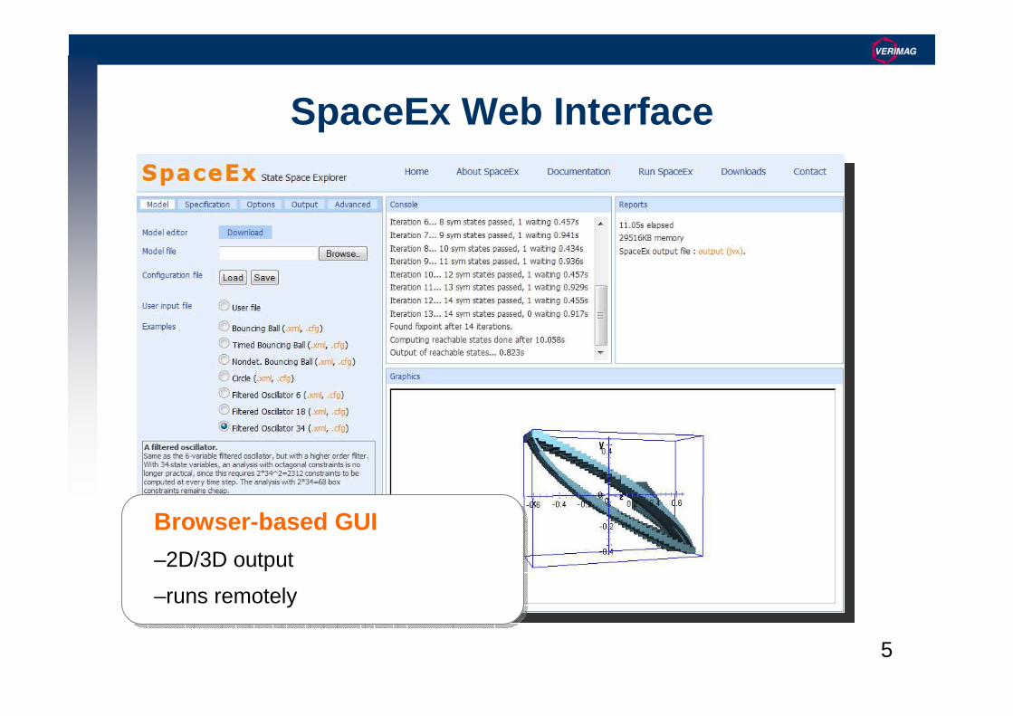
SpaceEx Web Interface
Browser-based GUI
–2D/3D output
–runs remotely

6
SpaceEx Reachability Algorithms
Support Function Algo
–many continuous variables
–low discrete complexity
PHAVer
–constant dynamics (LHA)
–formally sound and exact
Simulation
–nonlinear dynamics
–based on CVODE

7
linear differential equations
can be highly nondeterministic :
– additive “inputs” u,w model continuous disturbances (noise etc.)
– uncertain switching regions
– uncertain switch result
Hybrid Automata with Affine Dynamics
8
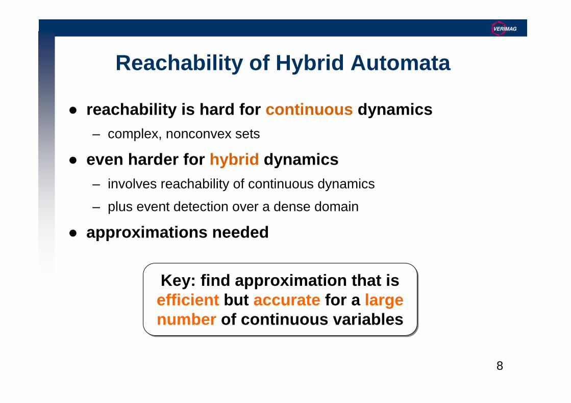
Reachability of Hybrid Automata
reachability is hard for continuous dynamics– complex, nonconvex sets
even harder for hybrid dynamics– involves reachability of continuous dynamics
– plus event detection over a dense domain
approximations needed
Key: find approximation that is efficient but accurate for a large number of continuous variables
Key: find approximation that is efficient but accurate for a large number of continuous variables
9
Outline
SpaceEx Verification Platform
SpaceEx Approximation Algorithm– Time Elapse Computation with Support Functions
– Transition Successors Mixing Support Functions and Polyhedra
– Fixpoint Algorithm: Clustering & Containment
Examples
10
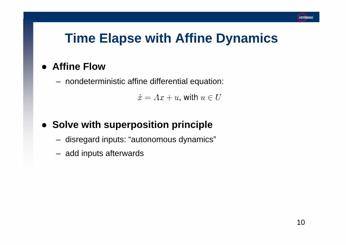
Time Elapse with Affine Dynamics
Affine Flow– nondeterministic affine differential equation:
Solve with superposition principle– disregard inputs: “autonomous dynamics”
– add inputs afterwards
11
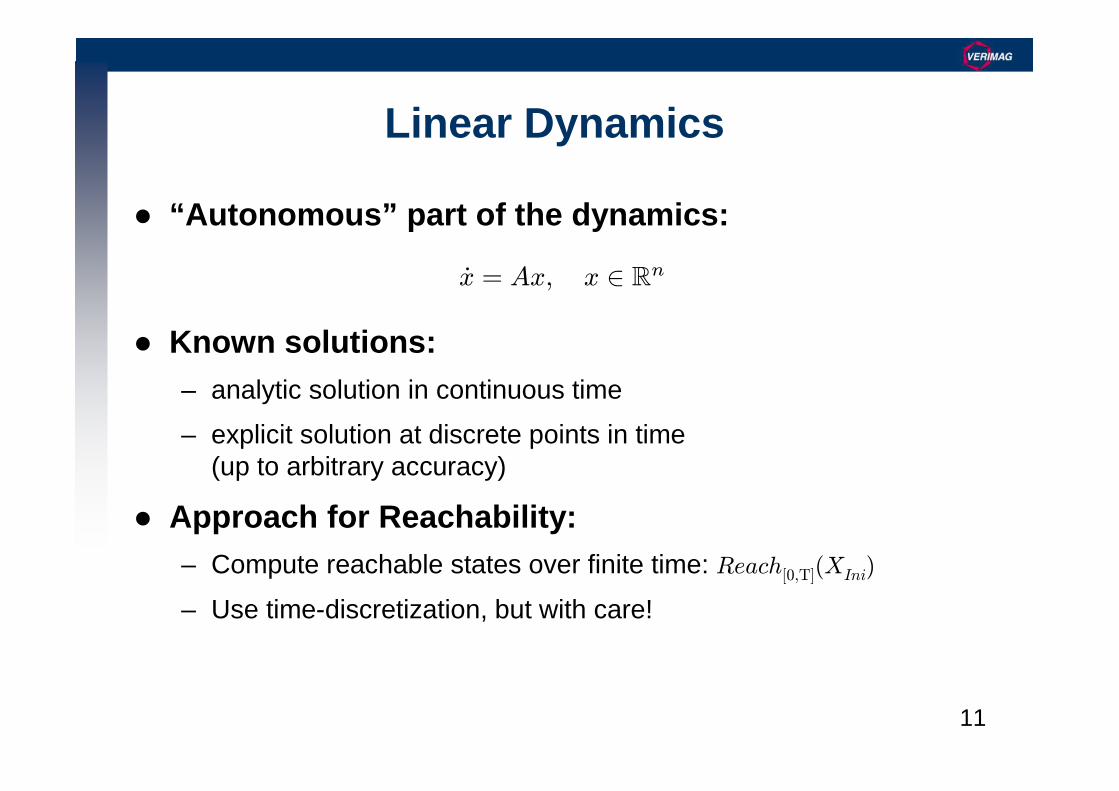
Linear Dynamics
“Autonomous” part of the dynamics:
Known solutions:– analytic solution in continuous time
– explicit solution at discrete points in time (up to arbitrary accuracy)
Approach for Reachability:– Compute reachable states over finite time: Reach[0,T](XIni)
– Use time-discretization, but with care!
x = Ax, x ∈ Rn

12
Time-Discretization for an Initial Point
Analytic solution:
Explicit solution in discretized time (recursive):x0 = xInixk+1 = eAδxk
x(t) = eAtxIni
2δ 3δδ0
x0x1
x2
x3
t
x(t)
multiplication with const. matrix eAδ
= linear transform
x(δ(k + 1)) = eAδx(δk)
• with t = δk :

13
Time-Discretization for an Initial Set
Explicit solution in discretized time
Acceptable solution for purely continuous systems– x(t) is in ǫ(δ)-neighborhood of some Xk
Unacceptable for hybrid systems– discrete transitions might “fire” between sampling times
– if transitions are “missed,” x(t) not in ǫ(δ)-neighborhood
2δ 3δδ0
X0
X1
X2
X3
t
X0 = XIni
Xk+1 = eAδXk
Reach[0,3δ](XIni)
14
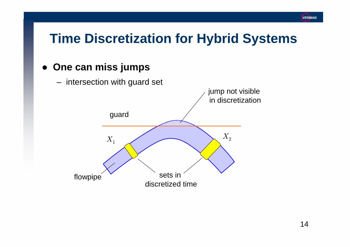
One can miss jumps– intersection with guard set
Time Discretization for Hybrid Systems
guard
flowpipe sets in discretized time
X1X2
jump not visible in discretization
15
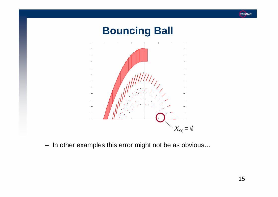
Bouncing Ball
– In other examples this error might not be as obvious…
X90= ∅
16
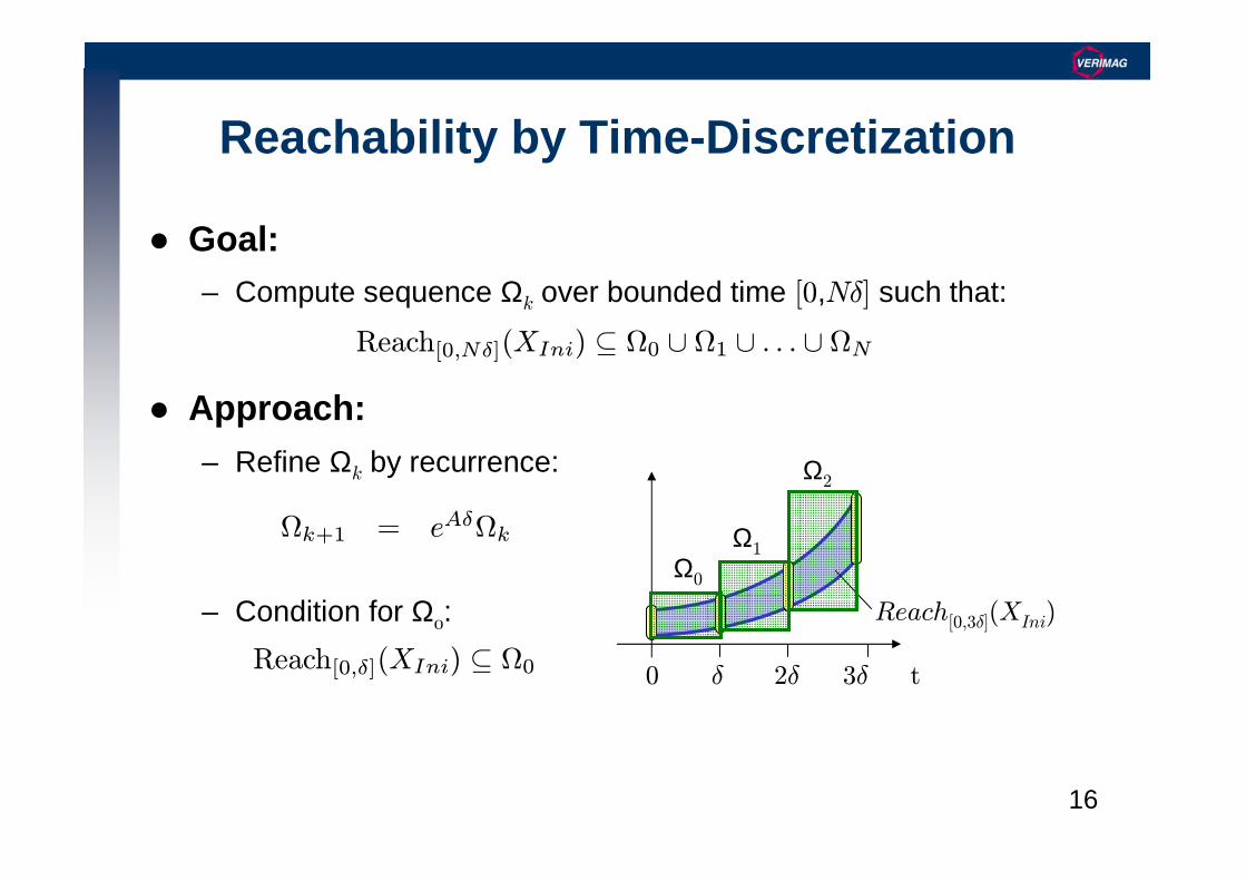
Goal:– Compute sequence Ωk over bounded time [0,Nδ] such that:
Approach:– Refine Ωk by recurrence:
– Condition for Ω:
Reachability by Time-Discretization
Reach[0,Nδ](XIni) ⊆ Ω0 ∪ Ω1 ∪ . . . ∪ ΩN
2δ 3δδ0 t
Reach[0,3δ](XIni)
Ω0
Ω1
Ω2
Ωk+1 = eAδΩk
Reach[0,δ](XIni) ⊆ Ω0
17
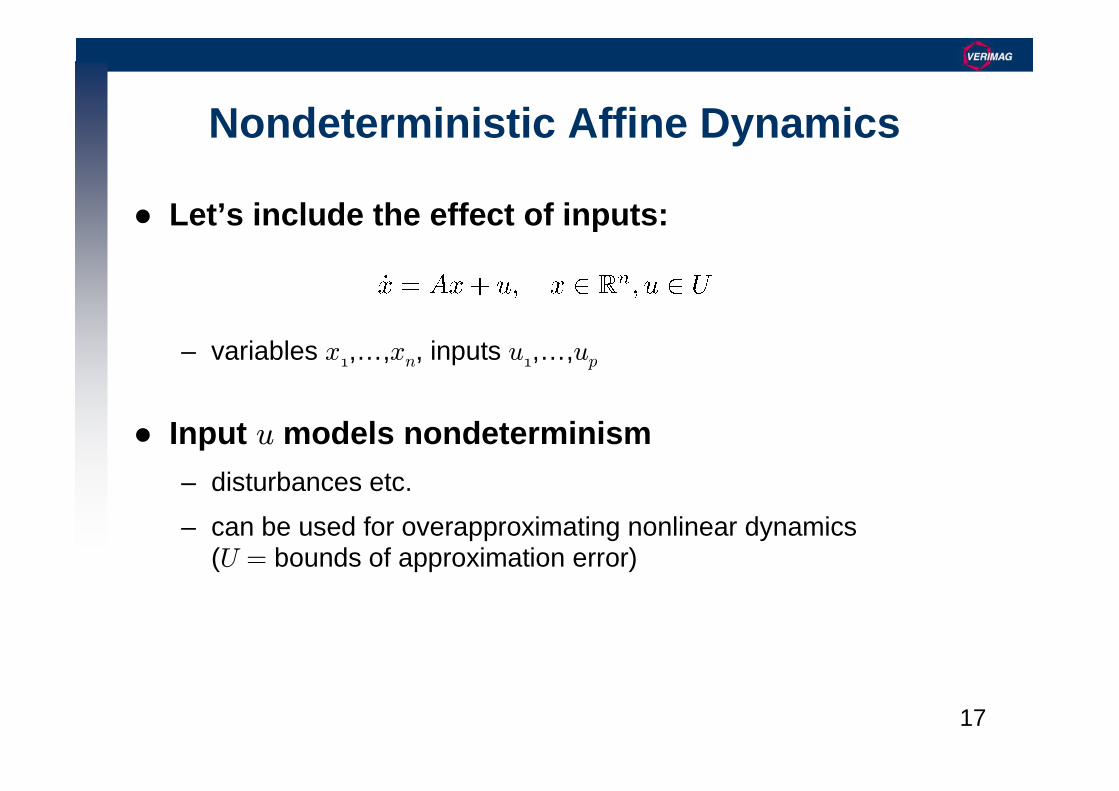
Nondeterministic Affine Dynamics
Let’s include the effect of inputs:
– variables x,…,xn, inputs u,…,up
Input u models nondeterminism– disturbances etc.
– can be used for overapproximating nonlinear dynamics(U = bounds of approximation error)

18
Nondeterministic Affine Dynamics
Superposition Principle
2δ 3δδ0 t
Reach[0,3δ](XIni)
influence of inputs
autonomousdynamics
influence ofinputs

19
Set overapproximation of input influence– How far can the input “push” the system in δ time?
– from Taylor series expansion
Operators:– Minkowski Sum:
– Symmetric Bounding Box:
– Linear Transform
Nondeterministic Affine Dynamics
A⊕B = a+ b | a ∈ A, b ∈ B
(error bound)
(matrix)
(input influence set)

20
Nondeterministic Affine Dynamics
Recurrence equation with influence of inputs
Still needed:– approximation of the
initial time step with Ω0
– called “approximation model”
2δ 3δδ0 t
Ω0
Ω1
Ω2

21
Approximation Models – Prev. Work
convex hull constraints + bloat with ∼∼∼∼ e||A||δ
Asarin, Dang et al., HSCC 2000
error large and uniform
exponential cost
bloat last set with ∼∼∼∼ e||A||δ
+ convex hull Le Guernic, Girard, CAV 2009
error large and uniform
efficient for high dimensions
X0 Xδ X0 Xδ

22
intersect forward and backward approximations
without inputs:exact at tttt=0=0=0=0 and tttt====δδδδ
approximate set for each tttt
+ bloat with ∼∼∼∼ eabs(A)δAX0
error small and non-uniformthanks to math tricks
New Approximation Model
Ωt
X0 XδX0 XδXt
23
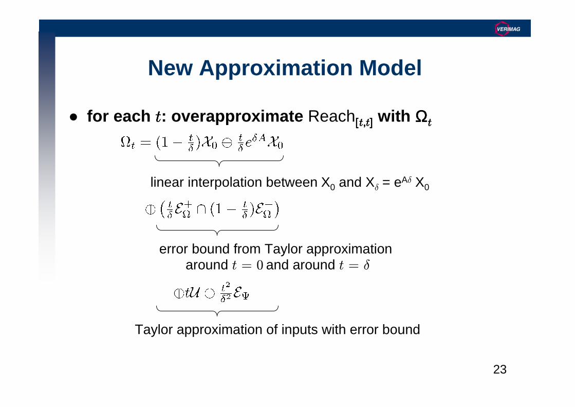
New Approximation Model
for each tttt: overapproximate Reach[[[[tttt,,,,tttt]]]] with ΩΩΩΩtttt
linear interpolation between X0 and Xδ = eAδ X0
error bound from Taylor approximation around t = 0 and around t = δ
Taylor approximation of inputs with error bound

24
New Approximation Model
overapproximate Reach[[[[0000,,,, δδδδ]]]] with convex hullof time instant approximations
error terms: symmetric bounding boxes

25
New Approximation Model
overapproximate Reach[[[[0000,,,, δδδδ]]]] with convex hullof time instant approximations
smaller overall error with math tricks– Taylor approx. of interpolation error
– bound remainder with absolute value sum instead of matrix norm

26
New Approximation Model
What Set Representation to Use?
Polyhedra
Operators Constraints Vertices Zonotopes Support F.
Convex hull -- + -- ++
Linear transform +/- ++ ++ ++
Minkowski sum -- -- ++ ++

27
Representing of Convex Sets
Approximation with Supporting Halfspaces– given template directions = outer polyhedral approximation
axis (± xi)⇓
bounding box2n facets
octagonal (± xi ± xj)⇓
bounding polytope 2n2 facets
all directions⇓
exact set
28
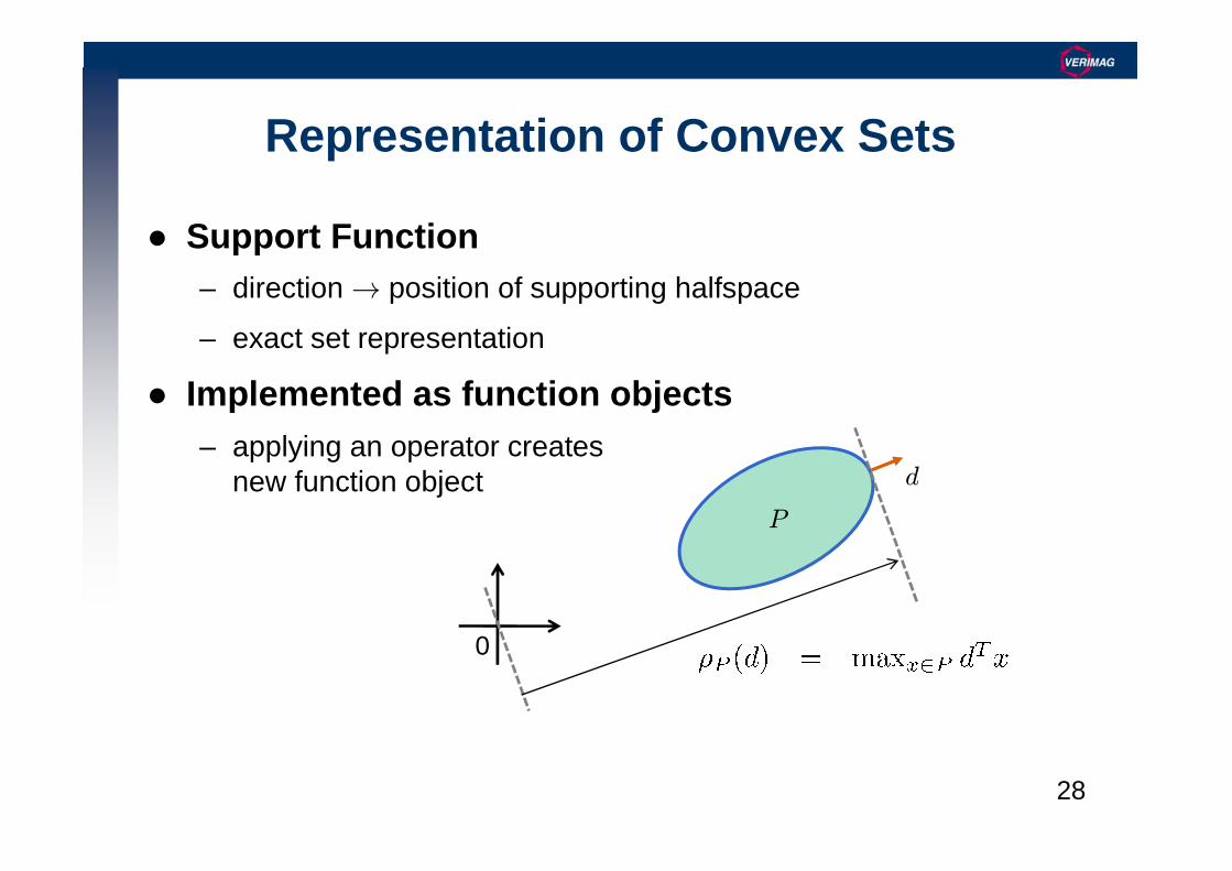
Representation of Convex Sets
Support Function– direction → position of supporting halfspace
– exact set representation
Implemented as function objects– applying an operator creates
new function object
0
d
P

29
Computing with Support Functions
Needed operations are simple
– Linear Transform:
– Minkowski sum:
– Convex hull:
Implement as function objects– can add more directions at any time
C. Le Guernic, A.Girard. Reachability analysis of hybrid systems using support functions. CAV’09
30
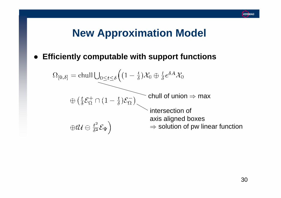
New Approximation Model
Efficiently computable with support functions
chull of union ⇒ max
intersection of axis aligned boxes⇒ solution of pw linear function
31
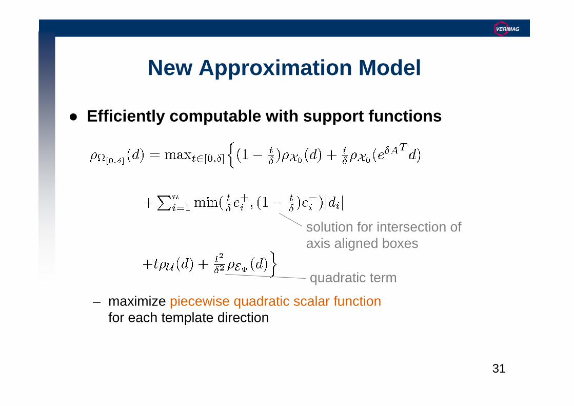
Efficiently computable with support functions
– maximize piecewise quadratic scalar functionfor each template direction
New Approximation Model
quadratic term
solution for intersection of axis aligned boxes
32
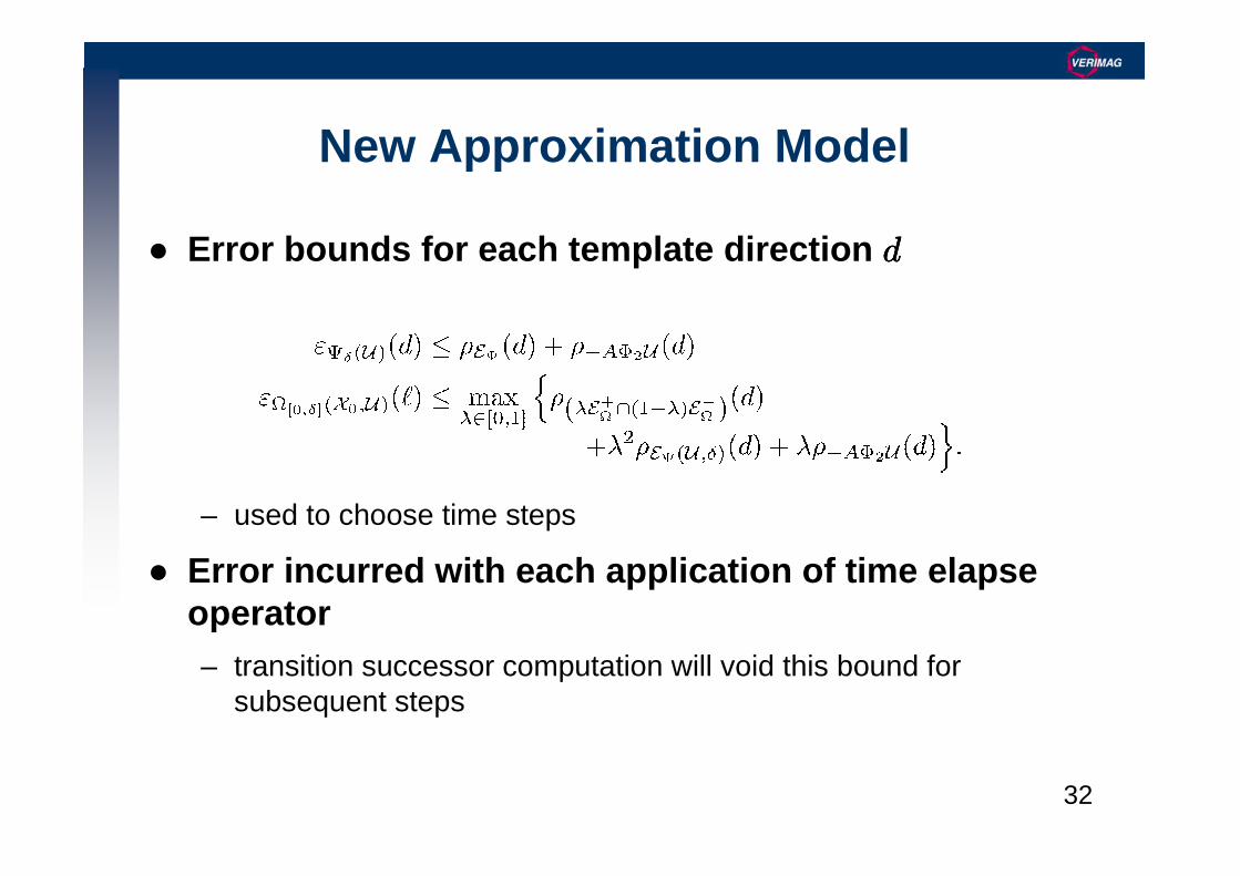
New Approximation Model
Error bounds for each template direction dddd
– used to choose time steps
Error incurred with each application of time elapse operator– transition successor computation will void this bound for
subsequent steps

33
Extension to Variable Time Steps
adapt to error
different time scale for each direction– new approximation model can interpolate
cost: recompute matrix eAδ
– cache matrix
X0
x
t2 t3t10 t
Ω0
Ω1
Ω2
34
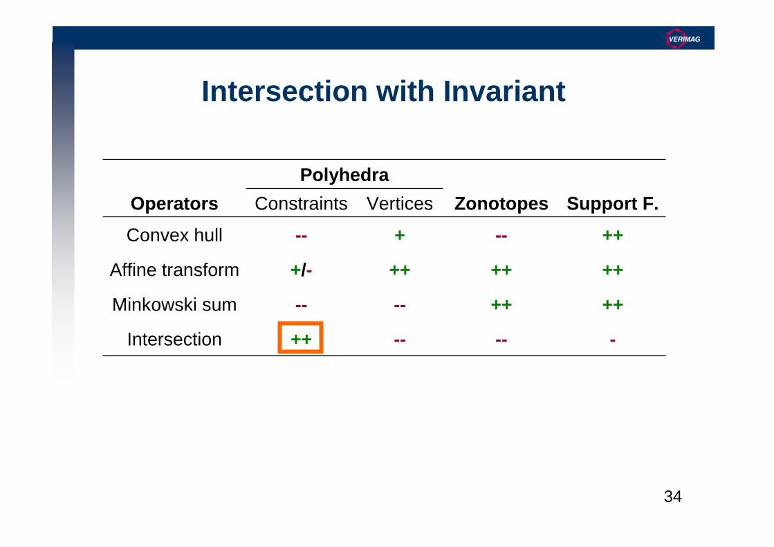
Intersection with Invariant
Polyhedra
Operators Constraints Vertices Zonotopes Support F.
Convex hull -- + -- ++
Affine transform +/- ++ ++ ++
Minkowski sum -- -- ++ ++
Intersection ++ -- -- -

35
Switching Set Representations
Classic example: Convex hull of polyhedra in constraint form– constraint form → vertex form: exponential cost
– compute convex hull in vertex form (union of vertices)
– vertex form → constraint form: exponential cost
Polyhedron →→→→ Support Function– cheap & exact: solve a linear program
Support function →→→→ Polyhedron– cheap, but overapproximative
– to bound Hausdorff distance: exponential # of template directions
36
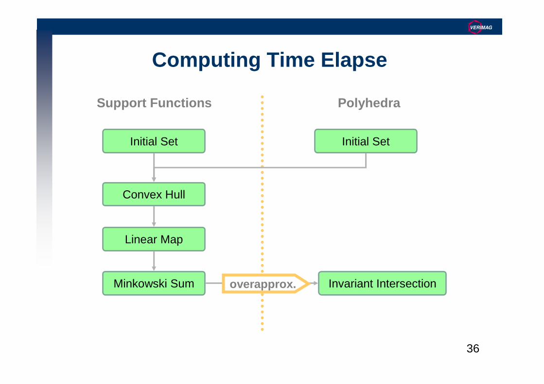
Computing Time Elapse
Linear Map
Minkowski Sum Invariant Intersection
Convex Hull
Support Functions Polyhedra
overapprox.
Initial Set Initial Set
37
Outline
SpaceEx Verification Platform
SpaceEx Approximation Algorithm– Time Elapse Computation with Support Functions
– Transition Successors Mixing Support Functions and Polyhedra
– Fixpoint Algorithm: Clustering & Containment
Examples

38
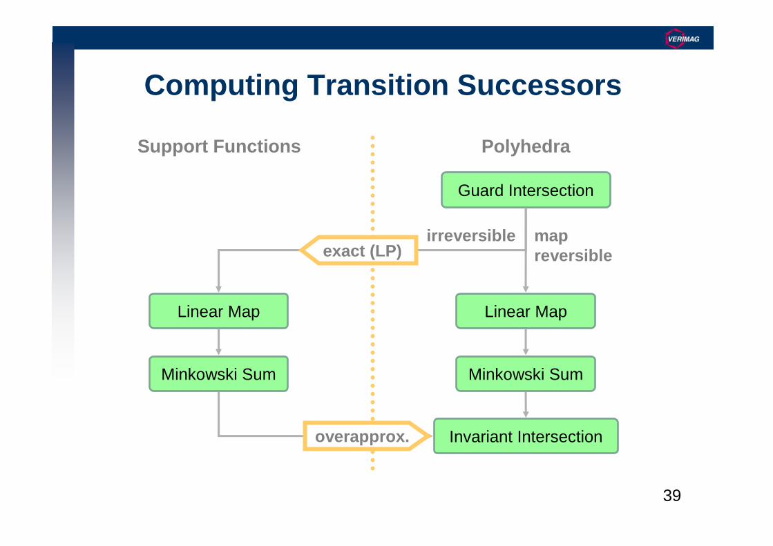
Computing Transition Successors
Intersection with guard– use outer poly approximation
Linear map &Minkowski sum– with polyhedra if invertible
(map regular, input set a point)
– otherwise use support functions
Intersection with target invariant– use outer poly approximation
x ≥ 0
bounce
x = 0 ∧ v < 0v := −cv
freefall
x = v
v = −g
x = x0
v = 0
guard
reset
39
Computing Transition Successors
Linear Map
Minkowski Sum
Invariant Intersection
Guard Intersection
Support Functions Polyhedra
overapprox.
Linear Map
Minkowski Sum
map reversible
irreversibleexact (LP)
40
Outline
SpaceEx Verification Platform
SpaceEx Approximation Algorithm– Time Elapse Computation with Support Functions
– Transition Successors Mixing Support Functions and Polyhedra
– Fixpoint Algorithm: Clustering & Containment
Examples
41
Fixpoint Computation
Standard fixpoint algorithm– Alternate time elapse and transition successor computation
– Stop if new states are contained in old states
Problem: flowpipe = union of many sets– number of flowpipes may explode with exploration depth
– containment very difficult on unions
Solution: – reduce number after jump through clustering
– use sufficient conditions for containment
– nested depth of support function calls is limited due to outer poly.
42
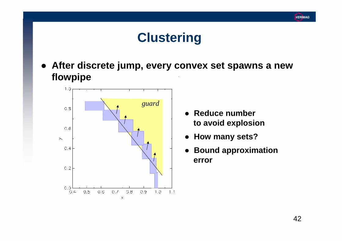
Clustering
After discrete jump, every convex set spawns a new flowpipe
Reduce number to avoid explosion
How many sets?
Bound approximation error
guard

43
Clustering – Template Hull
Template Hull = Outer polyhedron for template directoins
guard
template hull up to given error bound
⇒⇒⇒⇒ low number of sets
small error

44
Clustering
Even a low number of sets might be still too much
guard
2 sets ⇒⇒⇒⇒ possibly2k sets at iteration k
cluster again usingconvex hull
⇒⇒⇒⇒ 1 set, good accuracy
45
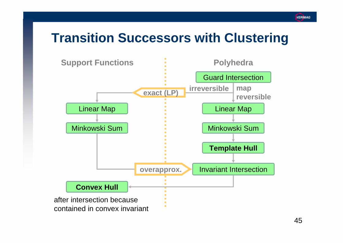
Transition Successors with Clustering
Support Functions Polyhedra
Invariant Intersectionoverapprox.
Linear Map
Minkowski Sum
Guard Intersection
Linear Map
Minkowski Sum
map reversible
irreversibleexact (LP)
Convex Hull
Template Hull
after intersection becausecontained in convex invariant

46
Sufficient Conditions for Containment
“Cheap” containment
– pairwise comparison
– comparison only with initial set of flowpipe
Clustering helps
– delays containment one iteration if clustering to a single set
47
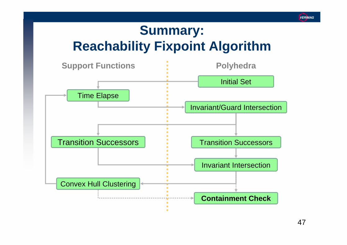
Summary: Reachability Fixpoint Algorithm
Invariant Intersection
Support Functions Polyhedra
Time Elapse
Initial Set
Invariant/Guard Intersection
Convex Hull Clustering
Transition SuccessorsTransition Successors
Containment Check

48
Outline
SpaceEx Verification Platform
SpaceEx Approximation Algorithm– Time Elapse Computation with Support Functions
– Transition Successors Mixing Support Functions and Polyhedra
– Fixpoint Algorithm: Clustering & Containment
Examples
49
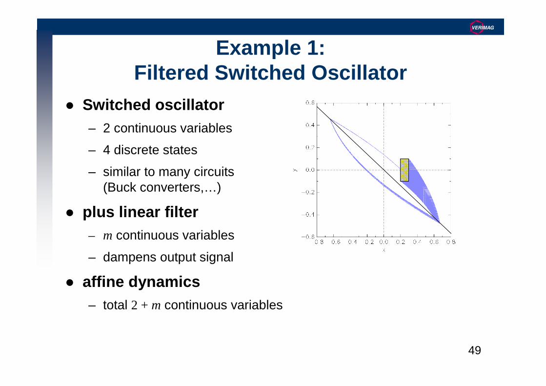
Example 1: Filtered Switched Oscillator
Switched oscillator– 2 continuous variables
– 4 discrete states
– similar to many circuits(Buck converters,…)
plus linear filter– m continuous variables
– dampens output signal
affine dynamics– total 2 + m continuous variables
50
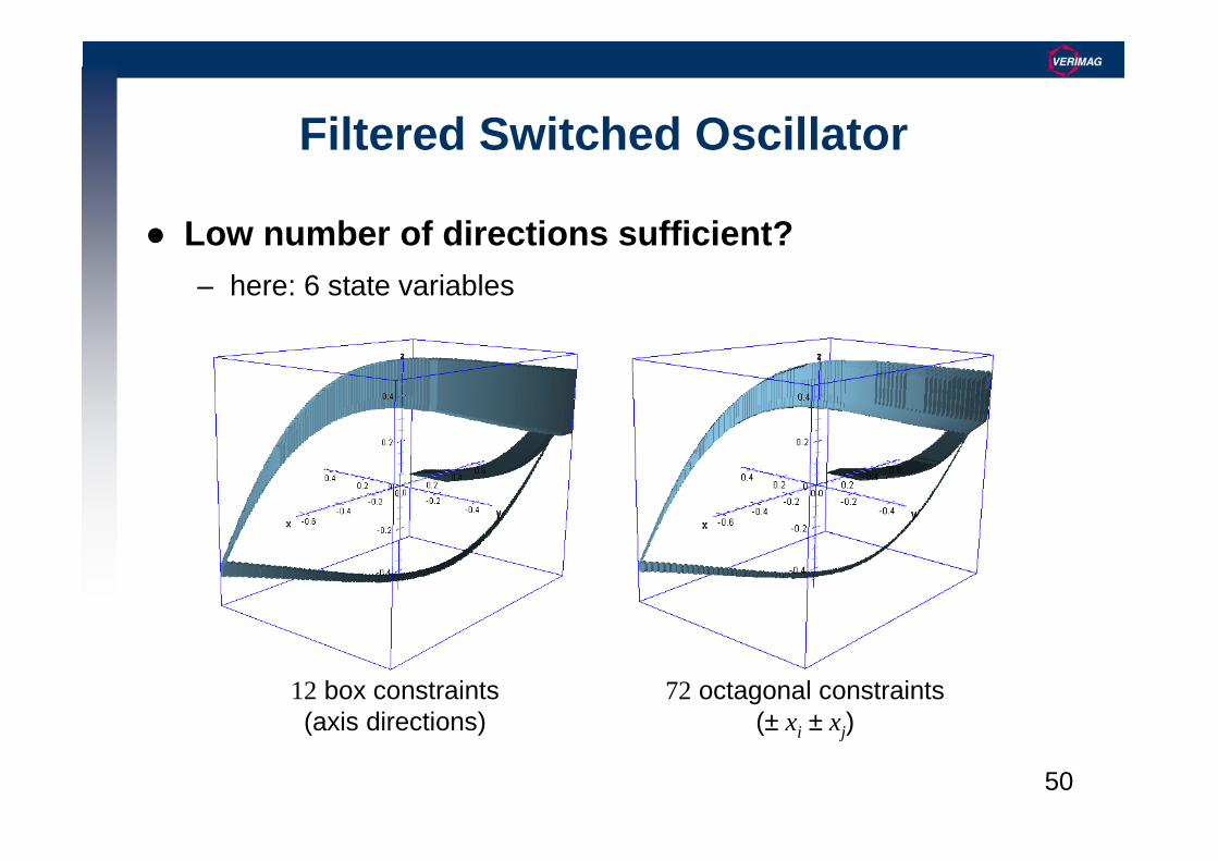
Filtered Switched Oscillator
Low number of directions sufficient?– here: 6 state variables
12 box constraints(axis directions)
72 octagonal constraints(± xi ± xj)

51
Example 1: Switched Oscillator
Connecting Filter Components
52
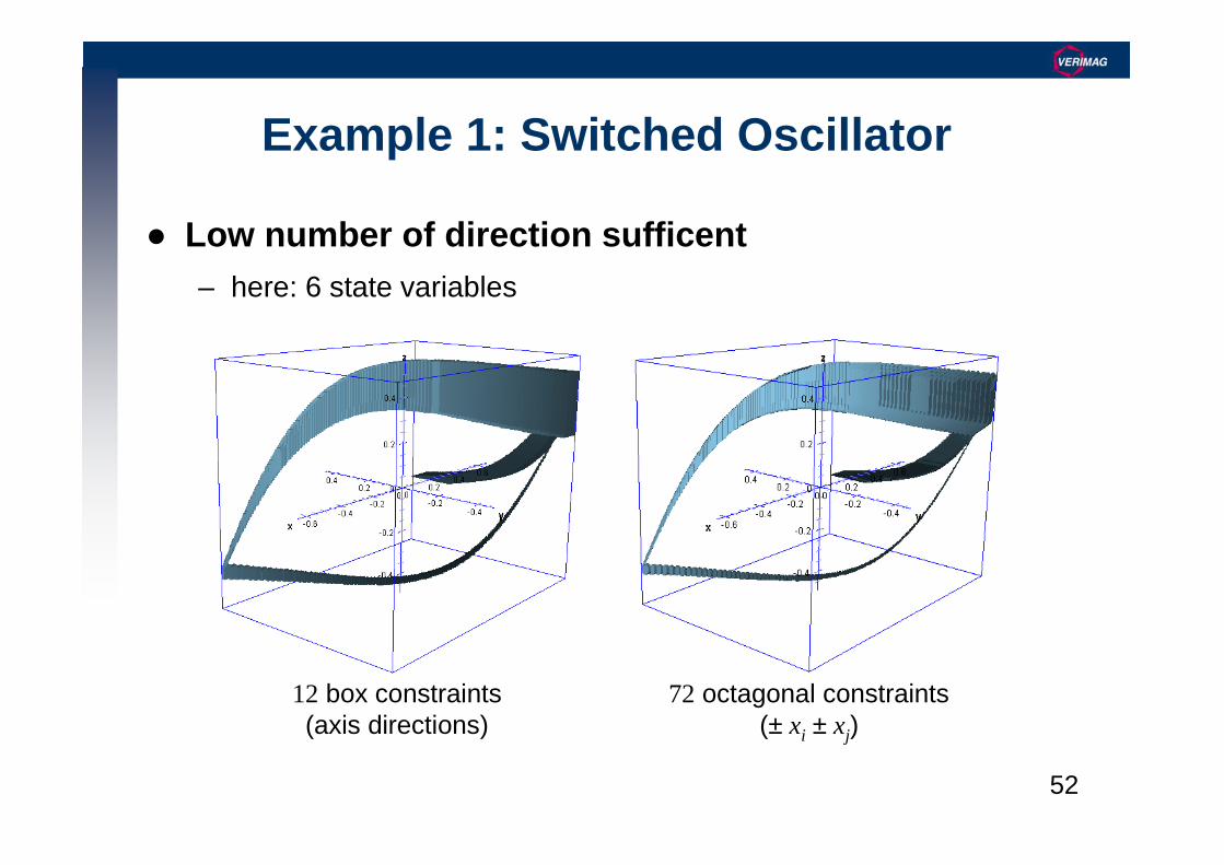
Example 1: Switched Oscillator
Low number of direction sufficent– here: 6 state variables
12 box constraints(axis directions)
72 octagonal constraints(± xi ± xj)

53
first jump has 57 sets ⇒⇒⇒⇒ impossible w/o clustering
Template Hull and Convex Hull Clustering
11.5 sec 3.6 sec
3.4 sec 8.2 sec
54
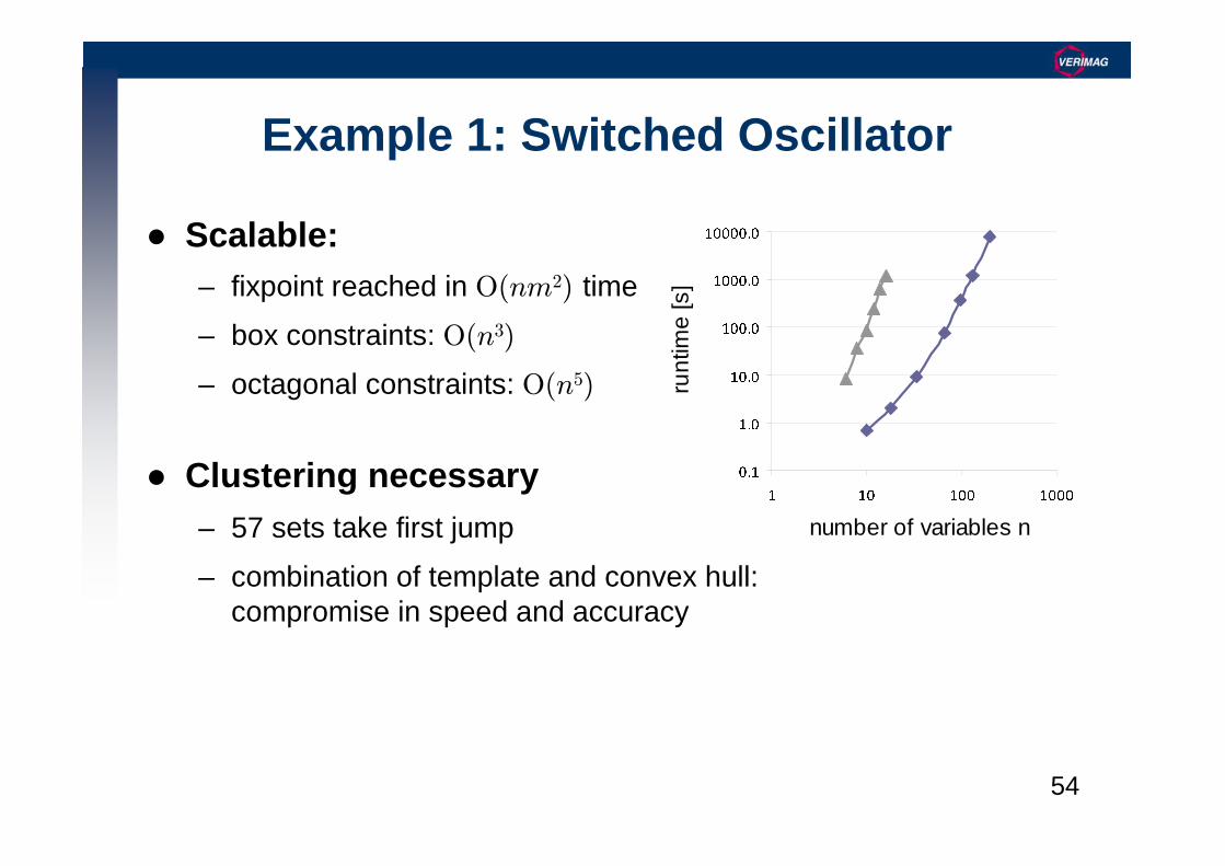
Example 1: Switched Oscillator
Scalable:– fixpoint reached in O(nm2) time
– box constraints: O(n3)
– octagonal constraints: O(n5)
Clustering necessary– 57 sets take first jump
– combination of template and convex hull:compromise in speed and accuracy
number of variables n
runt
ime
[s]

55
Example 2: Chaotic Circuit
piecewise linear Rössler-like circuitPisarchik, Jaimes-Reátegui. ICCSDS’05
added nondet. disturbances
3 variables, hard!

56
Example 2: Controlled Helicopter
28-dim model of a Westland Lynx helicopter– 8-dim model of flight dynamics
– 20-dim continuous H∞ controller for disturbance rejection
– stiff, highly coupled dynamics
S. Skogestad and I. Postlethwaite, Multivariable Feedback Control: Analysis and Design. John Wiley & Sons, 2005.
Photo by Andrew P Clarke

57
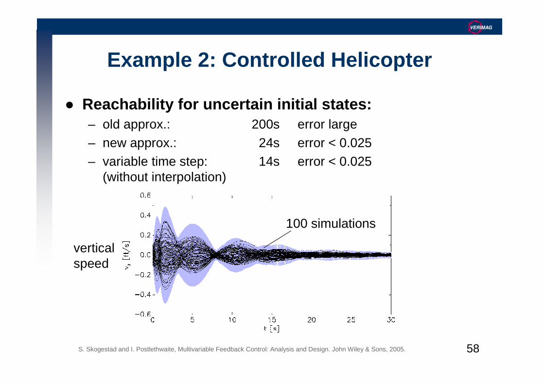
Example 2: Controlled Helicopter
Reachability for uncertain initial states:– old approx.: 200s error large– new approx.: 24s error < 0.025– variable time step: 14s error < 0.025
(without interpolation)
S. Skogestad and I. Postlethwaite, Multivariable Feedback Control: Analysis and Design. John Wiley & Sons, 2005.
verticalspeed
1 simulation
58
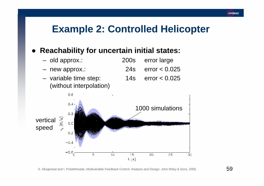
Example 2: Controlled Helicopter
Reachability for uncertain initial states:– old approx.: 200s error large– new approx.: 24s error < 0.025– variable time step: 14s error < 0.025
(without interpolation)
S. Skogestad and I. Postlethwaite, Multivariable Feedback Control: Analysis and Design. John Wiley & Sons, 2005.
verticalspeed
100 simulations
59
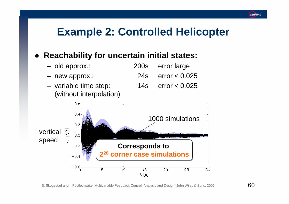
Example 2: Controlled Helicopter
Reachability for uncertain initial states:– old approx.: 200s error large– new approx.: 24s error < 0.025– variable time step: 14s error < 0.025
(without interpolation)
S. Skogestad and I. Postlethwaite, Multivariable Feedback Control: Analysis and Design. John Wiley & Sons, 2005.
verticalspeed
1000 simulations
60
Example 2: Controlled Helicopter
Reachability for uncertain initial states:– old approx.: 200s error large– new approx.: 24s error < 0.025– variable time step: 14s error < 0.025
(without interpolation)
S. Skogestad and I. Postlethwaite, Multivariable Feedback Control: Analysis and Design. John Wiley & Sons, 2005.
verticalspeed
1000 simulations
Corresponds to 228 corner case simulations
Corresponds to 228 corner case simulations
61
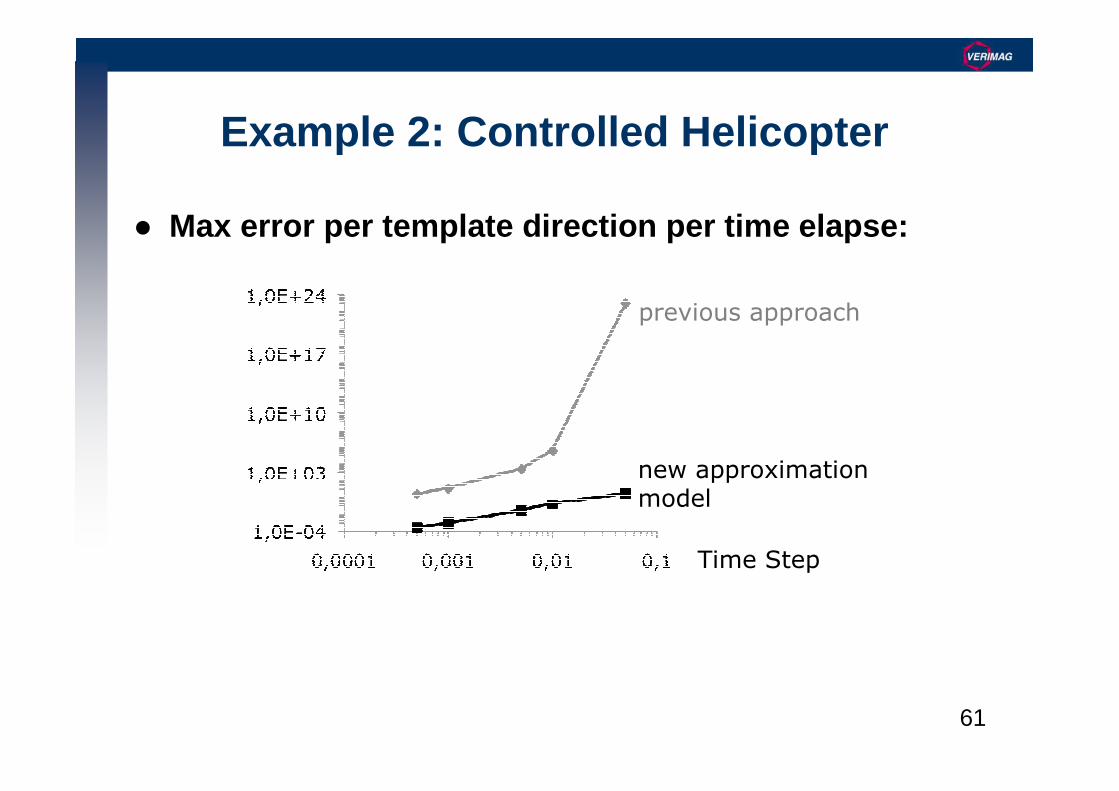
Max error per template direction per time elapse:
Example 2: Controlled Helicopter
Time Step
previous approach
new approximation
model

62
Max error per template direction:
Example 2: Controlled Helicopter
Time Step
previous approach
new approximationmodel
100x bigger time step for same error100x bigger time step for same error
63
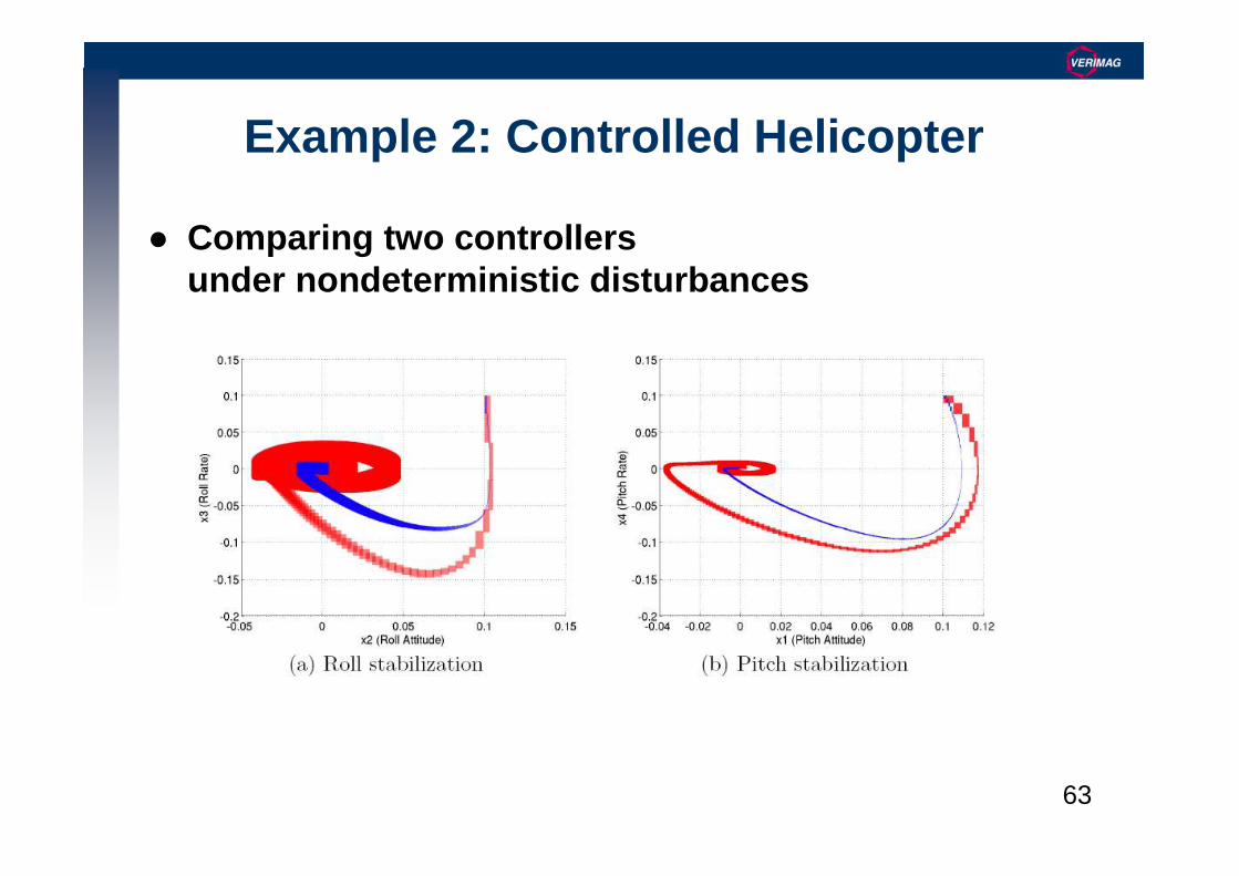
Example 2: Controlled Helicopter
Comparing two controllers under nondeterministic disturbances

64
Conclusions
SpaceEx Verification Platform– available at spaceex.imag.fr
– tutorial with solutions for course work
Scalable reachability for piecewise affine dynamics– fixpoint computation with 200+ variables
Algorithmic improvements– approximation improved significantly
– switching set representations for best efficiency
– variable time step with error bounds

65
Ongoing Work
Precise Intersection– reduce error by finding
template directions
Nonlinear Systems– linearize with sliding window
Tool Download: spaceex.imag.frTool Download: spaceex.imag.fr
66
Bibliography
Affine Dynamics– E. Asarin, O. Bournez, T. Dang, and O. Maler. Approximate
Reachability Analysis of Piecewise-Linear Dynamical Systems. HSCC’00
– A. Girard, C. Le Guernic, and O. Maler. Efficient computation ofreachable sets of linear time-invariant systems with inputs. HSCC’06
Support Function Reachability– C. Le Guernic, A.Girard. Reachability analysis of hybrid systems
using support functions. CAV’09
– G. Frehse et al. SpaceEx: Scalable Verification of Hybrid Systems. CAV’11