Safe Minimum Standards in Dynamic Resource Problems

Safe Minimum Standards in Dynamic Resource Problems—Conditions for Living on the Edge of Risk

Michael Margolis Eric Nævdal

February 2004 • Discussion Paper 04–03

Resources for the Future 1616 P Street, NW Washington, D.C. 20036 Telephone: 202–328–5000 Fax: 202–939–3460 Internet: http://www.rff.org

© 2004 Resources for the Future. All rights reserved. No portion of this paper may be reproduced without permission of the authors.

Discussion papers are research materials circulated by their authors for purposes of information and discussion. They have not necessarily undergone formal peer review or editorial treatment.


Michael Margolis and Eric Nævdal

Abstract Safe Minimum Standards (SMSs) have been advocated as a policy rule for environmental

problems where uncertainty about risks and consequences are thought to be profound. This paper explores the rationale for such a policy within a dynamic framework and derives conditions for when SMS can be summarily dismissed as a policy choice and for when SMS can be defended as an optimal policy based on standard economic criteria. We have determined that these conditions can be checked with quite limited information about damages and risks. In order to analyze the SMSs in a dynamic setting, we have developed a method for solving optimal control problems where the state space is divided into risky and non-risky subsets.

Key Words: safe minimum standards; optimal control; critical zone; threshold effects; mixed risk spaces.

JEL Classification Numbers: C61, Q20, Q30

Contents

1. Introduction......................................................................................................................... 1

2. A Dynamic Model of Safe Minimum Standards .............................................................. 4

Risk Thresholds in a Dynamic Context .............................................................................. 6 Optimization in the Presence of Risk Thresholds—A Conceptual Description ............7

When is a SMS Optimal?.................................................................................................. 10 Optimal Policies After a Catastrophe ..........................................................................12 Optimal Policies at the Risk Threshold .......................................................................12 Optimal Policies Prior to Reaching the Risk Threshold ..............................................16

Extensions ......................................................................................................................... 17 Uncertainty About the Location of Risk Threshold.....................................................17

Discussion and Conclusions ................................................................................................. 19

Appendix: Optimal Control in Mixed-Risk State Spaces. ................................................ 20

Deterministic Control Problems ....................................................................................... 20

Piecewise Deterministic Problems.................................................................................... 20

Jump Conditions for the Co-State Variables at the Risk Threshold ................................. 22

References.............................................................................................................................. 25


Michael Margolis and Eric Nævdal1

1. Introduction

Environmental and resource problems include many for which future damages are highly uncertain, possibly severe, and likely to be irreversible. In the public debate, a popular notion is that such problems should be dealt with by applying the Precautionary Principle (PP) and avoiding such risks altogether. PP seems to have great intuitive appeal both to the general public and to non-economist scientists. This may be why PP has been adopted in much environmental legislation, such as the Endangered Species Act and the Clean Water Act in the United States. Ciriacy-Wantrup (1952) suggested that such problems be addressed by establishing a Safe Minimum Standard (SMS) below which the flow of key ecosystem services should not be permitted to fall. To prevent an extinction, for example, we might establish a SMS for the size of the reproducing population, another for the area of its habitat, and a third (actually a safe maximum) for the extent of human activity within the habitat area. The concept of the SMS has since been refined in Bishop (1978,1979), Bishop and Ready (1990), and Crowards (1998) and put into practice in the form of critical habitat designation for endangered species, minimum flow and purity requirements for water quality, and others.

None of these arguments, however, is based on a conventional social welfare-maximization criterion, which makes SMS a controversial subject among economists. The cause of the controversy, as summed up by Farmer and Randall (1998), is that “SMS processes …cannot be derived from a single direct objective statement that also derives the policy exception upon which they are superimposed. ” The central contribution of this paper is to show that it is, in fact, possible to derive conditions under which an SMS policy will maximize social welfare and that surprisingly little information is required to verify whether these conditions hold.

1 Michael Margolis is a Fellow at Resources for the Future. He can be reached at [email protected]. Eric Nævdal is a research fellow, Department of Forest Sciences, at the Agricultural University of Norway. He can be reached at [email protected].

1

mailto:[email protected]

Resources for the Future Margolis and Nævdal

Economists have suggested alternative justifications for the use of an SMS. Most of these develop the philosophical position that there are limits beyond which utilitarian calculus ceases to be legitimate. Bishop’s (1978, 1979) case was built on the assumptions that planners are unaware of the probabilities of relevant events and that a planner ignorant of probabilities should follow a “minimax” strategy, which minimizes the maximum possible loss. This strategy is tantamount to assuming the worst possible outcome is a certainty and will not in general maximize welfare. Further investigation by Smith and Krutilla (1979) and Ready and Bishop (1991) uncovered several plausible circumstances in which abandoning a species to extinction is clearly preferable to an SMS. Bishop (1979) thus suggested the policy be abandoned when its cost is “intolerably” high, but there is no way to determine exactly how high a cost ought to be tolerated. Norton and Toman (1997) suggested an SMS could play a role in a “two-tiered” decisionmaking system, in which utilitarian calculus would give way to a more conservationist approach as irreversibility and justice issues increase in importance. This system would be a sort of compromise, or consensus, among utilitarians and partisans of other philosophical schools. In a similar vein, Farmer and Randall (1998) show that SMS is a common feature of agreements negotiated among citizens with varying moral positions.

Ciriacy-Wantrup (1952), however, based his original argument purely on discontinuities in the physical systems being managed or the models being used to predict those systems, rather than the philosophical framework used to value them. He recommended SMS as a management tool for what he called “critical zone resources,” a class in which he included animal and plant species, scenic resources, and the storage capacity of groundwater basins. The defining feature of this resource class was that the service flow could be smoothly manipulated at certain levels, but that beyond some critical zone a danger of collapse was introduced. Ecosystems often exhibit such threshold effects, at least at the level of resolution with which ecologists can understand them. For example, some species have minimum critical population thresholds such that a population will become extinct if population size goes below it. The location of this threshold will usually be imperfectly known. Another example is acid rain and eutrophication, which may lead to destruction or critical alteration of ecosystems if certain thresholds are violated (Mason 1996). In the case of acid rain, the increase in large-scale mortality risk is rapid as pH levels go below 4.5. Biologists and limnologists often treat these thresholds as deterministic, but since they are often site specific, the actual location of the threshold in any given ecosystem would be stochastic until a sufficiently extensive biological study of the relevant ecosystem had been conducted and a deterministic threshold established. It will however be a manageable task to

2


establish bounds where one can say that below2 such a bound, the probability of a catastrophe is zero. Such a bound is here referred to as a risk threshold.

The above are examples of risk thresholds created by the way in which natural scientists characterize problems. They can also be created by the way in which natural resource management is organized. Even if there is no bright line in the underlying risk, an SMS established by authorities at one level becomes a bright line for those whose compliance is being monitored. The U.S. Clean Air Act (CAA), for example, places local authorities in danger of losing control over economic development policy if the annual average concentration of any of several pollutants crosses a limit set by federal law. Thresholds for private sector decisionmakers are similarly induced by any regulation that places a firm in danger of increased regulatory scrutiny or litigation exposure conditional on an observable standard—for example, the Accidental Release Prevention rules of the CAA (EPA 1997).

Given a risk threshold from either natural or social sources, a manager is likely to consider using the threshold level as an SMS. Our task in this paper is to examine the circumstances in which this response is consistent with utilitarian calculus, thus redeveloping Ciriacy-Wantrup’s original argument with new rigor. We are especially interested in knowing when an SMS is a logical response to uncertainty. We derive conditions under which the optimality of a SMS can be determined in a cost–benefit analysis framework under the weakest possible assumptions. We show that an SMS is optimal policy if managers can put lower bounds on two parameters: the seriousness of the catastrophe and a parameter that determines how the magnitude of risk varies with the state-variable’s position in state space.

The present article examines SMSs in a dynamic context, reflecting our belief that this case is empirically the most important.3 The dynamic analysis of SMSs requires a division of state space into subsets with different risk structure. The boundaries between these sets are referred to as risk thresholds. We examine the particular type of problem where there is no risk in one subset of state space and risk in other subsets. In the risky subsets, the magnitude of the risk depends parametrically on the value of the state variables. We shall refer to state spaces that

2 The term “below the threshold,” as used here, is somewhat imprecise language and depends on the assumption that the probability of damage is a nondecreasing function, the function being strictly increasing if the argument is larger than the threshold. If the relevant variable is, for example, pH levels, where more is “good,” then “above the threshold” is the correct term. For simplicity, it is assumed throughout this paper that if a system is “below the threshold” then there is no risk. 3 Some results for static problems may be found in Nævdal & Margolis (2001).

3


are divided into risky and non-risky subsets as mixed risk spaces. To our knowledge, optimality conditions for this type of problem have not yet been analyzed in the literature. The technical challenge presented by this type of problem is that of finding conditions for the behavior of the co-state variables as the state variables crosses from one subset to another. We derive conditions for considerably more general problems than that of SMSs.

2. A Dynamic Model of Safe Minimum Standards

In this section, we consider the problem of managing a resource over time. Risk is represented by an event we term a “catastrophe.” We must associate the likelihood of this event with some specific risk structure. Obviously, the choice of risk structure depends on the real world interpretation of our model. Also, the choice of risk structure will influence the optimization framework that is used to solve the problem. The resource economic literature on optimal control in the presence of catastrophic risk can be roughly divided into two main categories. In one category, risk is modeled as a Poisson process where the catastrophic event has a probability distribution over time. The seminal paper for this model is, as far as we know, Dasgupta and Heal (1974). Heal (1991) and Clarke and Reed (1994) provide examples of this application. In the second category, risk is modeled as an event that occurs when a state variable exceeds some threshold in state space and the location of this threshold is unknown. In this approach, the event is distributed over state space. The seminal papers for this model are Cropper (1976) and Kemp (1976). Applications are provided by Tsur and Zemel (1995, 1996) and Nævdal (2003a). Nævdal (2003b) examines this type of problem for general ones where the threshold is a curve in n-dimensional space. The two approaches are superficially similar. For example both the Poisson type risk structure and the state-space distributed risk structure may take the form of probability distributions that depend on the paths of the state variables. Since the solution of a state-space distributed problem is found by converting such a problem to a Poisson type process, the necessary conditions for optimality are also quite similar. However the physical interpretations of the two types of problems are quite different. The relationship between these two approaches and the economic implications of the different risk structures are discussed in some detail in Nævdal (2003b). The approach chosen in this paper assumes that the risk structure is of the Poisson type where the catastrophic event is distributed over time. In its most general formulation, this implies that that the point in time at which a catastrophic event occurs has the following probability distribution: ( )( ) ( )( )( )0

,~ , exp t

s x s dst x t − λτ λ ∫ over . The intensity of +R

4


this distribution is given by λ(t, x(t)). The Poisson type risk structure is chosen for simplicity. Establishing the results below for state-space distributed events is straightforward.4

All the articles mentioned in the previous paragraph assume that the catastrophe takes the form of a discrete jump in instantaneous utility. Here we use an alternative approach, referred to as Piecewise Deterministic Optimal Control (PDOC), where the catastrophe takes the form of a jump in one or more state variables. The most important reason for choosing this approach is that the solution includes co-state variables that are directly commensurable with the co-state variables in deterministic control. This will be important in developing our results. The chosen approach also has the advantage that it is slightly more general. Not only can the method we use in the present article be used to analyze problems where there is a discrete jump in instantaneous utility, but it can also be used to analyze catastrophes where there are parametric shifts in the differential equations determining the paths of the state variables. Catastrophes where there are both jumps in instantaneous utility and the equations of motion may also be analyzed. PDOC is explained in Seierstad (2002) and reviewed in the appendix.

A possible source of confusion is that problems with events distributed over state space are occasionally given threshold interpretations. However, these thresholds are fundamentally different from the risk thresholds analyzed in this article. In the articles with state-space distributed risk, there is a shock of some sort when the threshold is crossed. In this article, the only thing that happens when the threshold is crossed is that the process becomes risky and a shock becomes possible.

4 There are of course other types of risk than catastrophic risk in resource economic problems, such as the case where movement in state variables is partly influenced by Brownian motion. However, SMSs are, to our knowledge, suggested as a policy only in cases where there is risk of catastrophic events. Brownian motion is used to model incremental risk. There exist hybrid models where there is both Brownian motion and catastrophic risk, such as Dixit and Pindyck (1994). Applying risk thresholds to these types of models is a possible extension not further discussed here.

5


Risk Thresholds in a Dynamic Context

This section explains how to give meaning to the concept of a risk threshold when state variables are functions of time. Let the state variables, x (t) ∈ R , evolve according to a the law

of motion

n

( ),x f x u= (1)

from a starting point denoted x (0) = x0. u∈ is a control function. If there is a catastrophe at some point in time τ, the state variable x jumps by a quantity g(τ, x(τ)). The arrival of this catastrophe is governed by a Poisson process with intensity

Rm

( )xΛ . Equation (2) defines this

process.

( )( )( )( )( )( )

Pr , | ( )

0 if 0( )

( ) if 0

t t t t x t

x tx

x x t

τ∈ + ∆ τ > ≈ Λ ∆

φ <Λ = λ φ >

(2)

x(t) represents the state of the resource at time t. The risk threshold is a curve in state space, defined by φ(x(t)) = 0, with φ(x(t)) < 0 being the safe side. If φ(x(t)) > 0 there is risk of the event t = τ occurring. The intensity λ(x) is assumed everywhere continuous and increasing5 except possibly when φ(x(t)) = 0. It is important to note that there is no physical jump in the variables as the state variables cross the risk threshold. The system goes from a subset of state space where there is no risk to a subset of state space where there is risk or vice versa. It is only if φ(x(t)) > 0 for a measurable amount of time that there is positive risk of a catastrophe occurring.

5 Some environmental variables are defined in such a way that an increasing numerical value reduces risk. This is the case for pH values whenever acidity represents an environmental problem. For such variables we would have to turn the definition around in an obvious way.

6


Optimization in the Presence of Risk Thresholds—A Conceptual Description

In the most general formulation of a risk threshold problem, we look for paths that solve the problem:

( )( )00max , rt

uE f x u e dt

∞ −∫ (3)

subject to the differential equation in (1) and the stochastic process in (2). f0 is the instantaneous utility depending on x and u. The problem defined by Equations (1) – (3) is may be envisioned as a sequence of decisions, where one solves a deterministic optimal-control problem whenever φ(⋅) < 0 and a piecewise deterministic problem whenever φ(⋅) > 0. Figure 1 illustrates this breakdown for the simplest possible sort of risk threshold—in which there is a time-invariant constant x separating the safe side from the dangerous side—is defined by φ(x(t))= x(t) – x ∀t. The horizontal line x is the risk threshold that divides the state space into subsets. Three paths are illustrated. These paths are not necessarily optimal, but serve to conceptualize the mathematical problem of optimizing in the presence of a risk threshold. ( )1x t is always below

the threshold. If this path is optimal, necessary conditions for optimality can be found with standard deterministic optimal control. If the path ( )3x t is optimal, then necessary conditions for

this path are found by applying PDOC. If the path ( )2x t is optimal, this follows from applying

standard deterministic control on the intervals [A, B], [C, D] and [E, ∞) and PDOC in the intervals [B, C] and [D, E]. It is important to note that the points in time where the risk threshold is crossed are endogenous to the problem.

7


x

x ( )1 t

x ( )3 t

x ( )2 t

t

x( )t

A B C D E

Figure 1. State-Variable Paths through a Mixed-Risk State Space

In fact, we need conditions for optimality for three types of problems:

1. Optimality conditions for the path after the catastrophe has occurred. We assume here that the catastrophe can only happen once and is irreversible. We therefore take the social-welfare maximization problem to be deterministic after the catastrophe has occurred.

2. Optimality conditions for the path if it is optimal to be in the deterministic subset of state space.

3. Optimality conditions for the path if it is optimal to be in the risky subset of state space.

8


Necessary conditions for optimality in the deterministic intervals are well known. Necessary conditions for PDOC are less well known and are given in the appendix. The remaining question is the behavior of the solution at the times the threshold is crossed. The state variable, x, simply follows the differential equation unless the catastrophe occurs. The behavior of the co-state variable is potentially subtler. This is an isoperimetric problem, since we require x(t) to be on a certain surface when the threshold is crossed. Such problems often have jumps in the co-state variables at any time T when the threshold is crossed. In the appendix, we show that whenever the threshold is crossed from a state where φ(⋅) < 0 to a state where φ(⋅) > 0, the co-state jump according to the following equation:

( ) ( ) ( ) ( )( )(

( )( ) ( )( ) (( ))0 0

1

, | ,

rTp T p T f f e p T f ff

)x T J T x g x J T xλ τ

− + + − − + + −−

+ + +

− = − + −

+ + − (4)

where T is the time when the threshold is crossed. p(⋅) is the co-state; and J denotes the criterion function evaluated at T. That is, J(T, x) = maxu ( )( )( )0 ,

T

rt dtE f x t u e∞ −∫ s.t. x(T) = x . Superscript

+ indicates that the function is evaluated at the limit from above and superscript − indicates that the function is evaluated at the limit from below. Thus ( )( ), |J T x g x τ+ + − is the loss

from the catastrophe if it happens at time T. It should be pointed out that these expressions are not assumed to be known, but are calculated recursively as a part of the necessary conditions. How is shown in Equation (34).

( ,+ )J T x

The expression for the case where the state goes from φ(⋅) > 0 to a state φ(⋅) < 0 is given by

( ) ( ) ( ) ( )( )(

( )( ) ( )( ) (( ))0 0

1

, | ,

rTp T p T f f e p T f ff

)x T J T x g x J T xλ τ

− + + − − + + −−

− − −

− = − + −

− + − (5)

The central insight from (4) and (5) is that there may be a jump in the co-state variable when x(t) crosses from one side of φ(·) = 0 to the other. As always, the co-state variable may be thought of as the shadow cost in terms of current and future welfare incurred when an additional unit of the state variable is made freely available. The discontinuous shift in this shadow cost at the threshold is an indication, although not a proof, that the intuition of the static example carries over to the dynamic. Sometimes one should reach the threshold and then stop, since the price of

9


going farther jumps, but this is never the case if the onset of risk is slow in the sense that if ( )xλ′ = 0 at the threshold.

If an SMS is applied then x = 0 for all t after the threshold has been reached. For this case, (4) and (5) are not well defined because their derivation involves division by ( )x T + = 0.

When an SMS is applied, the co-state will jump according to

( ) ( )( ) ( ) ( )( )( ) ( ) ( ) ( )( )( )

( ) ( ) ( )( )( )0 0, , , , , , , ,

, , , ,

f T x T u T x T p T f T x T u T x T p Tp T p T

f T x T u T x T p T

+ + + + + − − − − −

− +

− − − − −

−− = (6)

That is, the jump in the shadow cost of resource damage is the jump in instantaneous social welfare divided by the speed with which the state variable is changing as the threshold is approached.

When is a SMS Optimal?

We now turn to the question of when an SMS is optimal. To dispose of the trivial problems, assume x0 is on the safe side of the threshold and that the path of x will cross the risk threshold if no action is taken to regulate the resource. We must first define what is meant by a SMS in a dynamic context. One possible definition is simply to require that φ(x(t)) ≤ 0 ∀t. This is essentially what we shall mean by a SMS.6 A policy obeying a SMS would have to look something like Figure 2. In the interval [0, T) the system is approaching the risk threshold. In the interval [T, ∞), the SMS is binding. The similarity to a Most Rapid Approach path in linear

6 Strictly speaking, a slightly more general definition is possible and, as argued below, in fact, required if necessary conditions are to hold. Defining Ψ(t) = λ(x(t)) if φ(x(t)) > 0 and Ψ(t) = 0 if φ(x(t)) < 0. A path will be considered able to satisfy a SMS from the time s if and only if the Lebesque integral

shas measure zero. This means

that we may allow the threshold to be violated as long as the violations are not large enough to give positive probability to the possibility that the catastrophe occurs. Thus, an SMS can include a policy of forcing the system back below the threshold as soon as the policy is seen to have crossed it, provided the observation and reaction is instantaneous. An infinite number of such jumps may be allowed and will, in certain circumstances, be required if a path is to observe necessary conditions. This point is further discussed below.

( )t dt∞Ψ∫

10


optimal control problems is superficial. If a path such as the one in Figure 2 is optimal, then the flattening in the path of x is caused by the jump in the co-state variable at time T.

Our strategy for examining the optimality of an SMS is as follows. We assume that the solution is qualitatively similar to the path in Figure 2. We then use necessary conditions to examine for what parameter values such a path is consistent with optimality. For clarity we derive our results within a parameterized model. Let the equation of motion be

( , )x f x u u xδ= = −

0a =

; let the constant A be a net utility cost that is accrued if the catastrophe

occurs. Formally this implies that we define a state variable a(t). The differential equation for this equation is , a(0) = 0. If the catastrophic event occurs, a(τ+) – a(τ-) = –A. Let the intensity of the catastrophe process be the quadratic function λ(x) = ( ) ( )20 1x x xλ λ x− + − for all x ≥ x , where λ1 is strictly positive. The instantaneous cost of reducing u is given by 2

c (u0 –

u) . 2

x

T t

x( )t

Figure 2. State-path satisfying SMS.

11


The objective function that we want to maximize is then given by:

( )( )202

0

rtcE u u a e∞

−− − +∫ dt (7)

Optimal Policies After a Catastrophe

In order to characterize the solution, we need to find the post-catastrophe solution. In the present example, this is equivalent to solving the problem

( ) ( )( )202, * | max rtc

uJ x a A u u A e d

∞ −

ττ = = − − −∫ t

)

(8)

subject to , x(τ) = x*. is the value of the objective function from the

time, τ, that the catastrophe occurs and there is a flow, –A, of disutility. x* is interpreted as the value of x at the point in time when a catastrophe occurs. This problem has the trivial solution u = u0 for all t > τ. After all, the catastrophic event has already happened so there is no need to reduce x. Inserting u = u0 into equation (8) gives that J(x*|τ) =

x u x= − δ ( , * |J x a Aτ =

1 rr Ae− − τ− for all values of x*. In particular, note that J( x |τ) = . This is the discounted value of receiving a stream of negative utility from the time τ if x is at the threshold.

1 rr Ae− − τ−

Optimal Policies at the Risk Threshold

The next step is to find the optimal solution for the interval [T, ∞), given that the catastrophe has not occurred. This is the interval where the state is in the risky region prior to the catastrophe occurring. T is as yet not determined, but should be thought of as the point in time when the risk threshold is crossed. By the principle of optimality, the results below will hold for any arbitrary choice of T as long as x(T) = x . The problem at hand is to solve:

12


( ) ( )( )( ) ( ) ( ) ( )

( )( ) ( ) ( ) ( )( )

202

20 1

, | 0 max

. . : , 0, , ,

Pr , |

u

rtc

T

J T x a E u u a e dt

s t x u x a x T x a T A a a A

t t t x x x t x x x x t

∞−

+ −

= − − +

= − δ = = = τ − τ = −

τ∈ + ∆ ≥ ≈ λ ∆ = λ − + λ − ∆

∫ (9)

All constants are assumed strictly positive except, possibly, λ0. It is assumed that the shape of λ is such that λ′ ≥ 0 for all feasible values of x. The Maximum Principle for PDOC problems is given in the appendix. Using (30) to derive the first order conditions gives:

0 rtxpu u ec

−= + (10)

( ) ( )( ) ( ) ( ) ( )( )| , | 0 ,x x x x |p p x p p t t x J t x a J t x a Aδ λ τ λ′= + − > + = − = (11)

0 rtpx u ec

xδ−= + − (12)

( )xp t is the present value co-state variable for x.7 ( ), |J t x a A= is the criterion evaluated from

time T given that the catastrophe has occurred. This expression was defined in (8). ( ), | 0J t x a =

is the expected value of the criterion given that the catastrophe has not occurred. In general, is determined by the differential equation in (34) and quite complicated to solve.

However, we are examining the optimality of a SMS, and if a SMS is optimal, we can use the following reasoning to simplify the calculations. If the SMS is optimal, then the solution stays at the threshold and λ(x(t)) = λ(

( 0a = ), |J t x

x ) = 0 for all t ≥ T. The calculation of ( ), |J t x a A= is then

straightforward:

( ) ( ) ( )20 0, | 02 2

rt rT

T

c cJ T x a u x e dt u x er

∞ 2− −= = − − = − −∫ δ δ

(13)

7A co-state variable for a(t) also may be computed, but does not affect the solution and has no important economic interpretation. Discussion of this variable is therefore omitted.

13


For all t ∈ [T, ∞) we get the quantities ( ), | 0J t x a = and ( ), |J t x a A= by substituting τ

with t in (8) and T with t in (13). Let ( ) ( ) rtx t ex t pµ = be the current value co-state. If the optimal

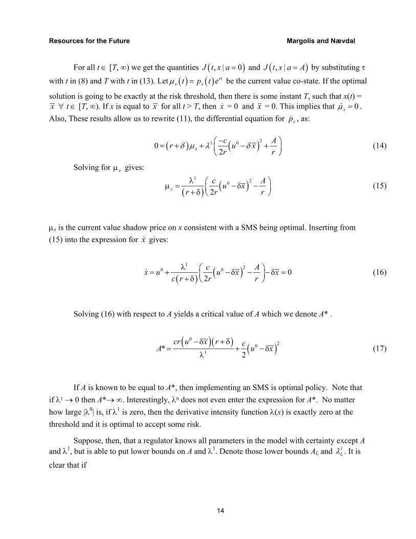
solution is going to be exactly at the risk threshold, then there is some instant T, such that x(t) = x ∀ t ∈ [T, ∞). If x is equal to x for all t > T, then x = 0 and x = 0. This implies that 0xµ = . Also, These results allow us to rewrite (11), the differential equation for xp , as:

( ) ( )21 002x

cr u xr r

δ µ λ δ−= + + − +

A (14)

Solving for µ gives: x

( ) ( )

1 20

2xc u x

r rλ µ = −δ −+ δ

Ar (15)

µx is the current value shadow price on x consistent with a SMS being optimal. Inserting from (15) into the expression for x gives:

( ) ( )

1 20 0 02c Ax u u x x

c r r rλ = + − δ − − δ = + δ

(16)

Solving (16) with respect to A yields a critical value of A which we denote A* .

( )( ) (

020

1*2

cr u x r cA−δ + δ

= +λ

)u x−δ (17)

If A is known to be equal to A*, then implementing an SMS is optimal policy. Note that if λ1 → 0 then A*→ ∞. Interestingly, λ0 does not even enter the expression for A*. No matter how large |λ0| is, if λ1 is zero, then the derivative intensity function λ(x) is exactly zero at the threshold and it is optimal to accept some risk.

Suppose, then, that a regulator knows all parameters in the model with certainty except A and λ1, but is able to put lower bounds on A and λ1. Denote those lower bounds AL and 1

Lλ . It is

clear that if

14


( )( ) (

020

1 2LL

c u x r cAr

− +≥ +

δ δδ

λ)u x− (18)

then it will always be optimal to let the SMS be binding from some point in time. If lower bounds can be established for the relevant parameters A and λ1 and these obey (18), then a SMS policy will be optimal. These findings are summed up in Proposition 1.

Proposition 1.

Consider problem (9). If A and λ1 are random variables with lower bounds AL and 1Lλ and

it can be established that AL and λ obey the inequality in equation (18). Then there exists some

point in time, T, such that the risk threshold is binding and a SMS policy is optimal.

1L

Note that (18) is a sufficiency condition, but not a necessary condition for a SMS to be binding. If a regulator is able to form a probability distribution over possible values of A, then a SMS may be optimal if E(A) ≥ A* even if A < A* with some probability. The current value cost of implementing a policy that satisfies a SMS from the time t = T is given by:

( 0

2cC ur )x= −δ (19)

From (18) it is evident that we find a lower bound for when the cost of accepting a SMS becomes intolerably high. Rewriting (18) gives us the following condition:

( ) ( )( )020

12 LL

c u x rc u x C Ar

− δ + δ− δ = ≤ −

λ (20)

The lefthand side is current value cost of a SMS. The right hand side is the ex ante lowest possible cost of allowing the state variable increase marginally above the risk threshold. If C is so high that (20) does not hold, then the SMS may be too high.

It is interesting to note that calculating the optimality of a SMS requires less information than is required to calculate the optimal path if we know that SMS is not optimal, for example, if λ1 = 0. For that, we either need to know A (and all the other parameters) exactly or we must at

15


least be able to form meaningful probability distributions over the values they may be able to take. What we have derived is one structure of uncertainty—perhaps not only one—that can justify the application of an SMS on purely utilitarian grounds. This is true uncertainty in the sense of (Knight, 1921) The probability of catastrophe is not known, although a lower bound for it is.

There is a technical issue concerned with how to characterize an optimal solution if we know that A > A*. That is, the cost of a catastrophe is strictly larger than the minimum cost required for the optimality of SMS. If this is the case, then a path with x = 0 does not, strictly speaking, satisfy necessary conditions. The optimal ( )x T + < 0 and will therefore be bounded

towards the no-risk region. But as soon as we enter the no-risk region any path that satisfies necessary conditions is bounded towards the risk region. This is resolved by letting the control be a chattering control, which means one that is discontinuous at every point in time after the threshold has been reached. See Zelikin and V.F. Borisov (1994) for an extensive discussion of chattering controls. The control will jump according to (4) and (5) in such a way that whenever x > x , then x < 0 and vice versa. The SMS will then be observed in the sense discussed in footnote 7. This is obviously an impractical control, but in the present context there is little loss from ignoring this issue when the threshold is reached and simply setting u = δ x at the threshold and thus keeping x at the threshold forever. However, see Nævdal (2001) for a deterministic threshold model where chattering is a fundamental and unavoidable property of the control.

Optimal Policies Prior to Reaching the Risk Threshold

So far we have examined the path the optimality of a path satisfying a SMS from the time the system reached the risk threshold. If A and λ1 are known with certainty to have values such that (17) holds with equality, this would be a straightforward procedure. A jump in the co-state variable could be calculated according to (6) and p(T-) be solved from:

.

( ) ( ) ( ) ( ) ( ) ( )( )( )

21 220

1 20

0

1 12

2

rT rT

rT

c Au x e P T ec r r r cc Ap T u x

r r r P Tu e x

c

− −

−−

−

λ − − δ − + + δ λ − + − δ − = + δ − − δ

−

(21)

16


Calculating the u(t), x(t) prior to T and T itself would be a straightforward, if algebraically tedious, problem. However, if we base the optimality of a SMS on lower bounds derived from (18) and do not have any more information about A and λ(x), then we cannot calculate the optimal path prior to reaching the SMS. In this case, we must form expectations about relevant parameters, no matter how vaguely founded, and approach the risk threshold as best we can. It should, however, be noted that, in most cases where a SMS is considered as a policy option, optimal policies prior to reaching the risk threshold are generally considered problems of secondary importance, if discussed at all.

The model discussed here has a linear differential equation. This is a simplification, in particular as the many natural systems where a SMS is a potential policy exhibits very nonlinear behavior. This is a fairly innocuous assumption as far as evaluating the optimality of a SMS. Allowing for a nonlinear differential equation only increases the algebraic complexity. As long as we can recursively calculate the co-state variable and the value of J(⋅|τ), we can use the jump

equations in (4) and (5) and check for the optimality of an SMS in the way described above. More important is the choice of functional form of λ(x), since the value of parameter λ1 turned out to be crucial. The choice of the quadratic function implies that λ(x) may be considered a Taylor expansion of the underlying risk structure. The coefficient for the quadratic term, λ0, disappears from the Equation (18). In fact, for any choice of polynomial, only the first order coefficient will matter. Hence, no matter how nonlinear the risk structure is, this does not impact the results. This argument does however assume that the underlying risk structure is continuous, which appears to be the most relevant case.

Extensions

Here we briefly discuss two possible extensions of the theory that may have some empirical relevance.

Uncertainty About the Location of Risk Threshold

So far the paper has assumed that the location of the risk threshold, x , is known to the regulator. In many cases this is not the case. It could be that the definition of Λ(x) would have to

17


be modified to take account for a stochastic x with support [ Lx , Hx ] ⊂ [0, ∞). It turns out that

the results derived above can be modified if we replace Λ(x) (and therefore also λ(x)) with a modified risk process given by

)

0

t∆

<

>

( )( )( )( )( )( )

Pr , | ( )

0 if 0( )

( ) if 0

t t t t x t

x tx

x x t

τ∈ + ∆ τ > ≈ Λ ∆

φ <Λ = λ φ >

(22)

Here φ(x) = x(t) – xL and ( ) ( ) (20 1Lx x x x xλ = λ − + λ −

). The algebraic procedure to

needed to translate Λ(x) to (xΛ may be quite complicated, but once this task has been

achieved, the results from above follow directly.

L

Mixing Endogenous and Exogenous Risk

For some problems where a SMS may be a policy option, it may be the case that there is underlying risk that is independent of human activity. For instance, there may be a risk that a population of a threatened species may collapse even in the absence of human interference. This could be modeled by using a risk structure of the following type:

( )( )( ) ( )( )

( ) ( )( )

Pr , | ( )

if 0( )

( ) if

t t t t x

t x tx

x t x t

τ∈ + ∆ τ > ≈ Λ

ω φΛ = λ +ω φ

(23)

Here there is some underlying stochastic process, ω(t), that may trigger the catastrophe.

By using the methods in the appendix, it is straightforward to analyze the optimality of SMSs also when (23) drives risk. It turns out that in our model this does not affect the decision of whether a SMS is optimal or not. The condition in Equation (18) remains the same. Of course, a SMS is not strictly “safe” anymore. Rather, it is a decision not to impose more risk on a natural system than that which is already inherent in the natural functioning of an ecosystem. Modeling the risk structure in this way would make the SMS as it here defined closer to the concept of a Minimum Viable Population as it defined in Soule (1987).

18


Discussion and Conclusions

The paper has analyzed the likelihood of a Safe Minimum Standard (SMS) being optimal policy in environmental regulation. Our most significant result is that one can establish a relationship between a lower bound on the damage and a lower bound on a crucial parameter in a pdf [a pdf file? confusing – probability density function – should be clear to the intended audience]that models uncertainty above a risk threshold. This is the first result to show that there are any circumstances in which an SMS can be dictated by a conventional social-welfare maximization criterion, rather than the minimax or nonutilitarian arguments resorted to by earlier authors. An important feature is that little knowledge about the nature of a catastrophe is required. Also, as mentioned in the introduction, such stark thresholds are often created by federal systems. Thus, it may well be optimal for a state regulator to impose an SMS on local polluters, given that the federal government has created an air-quality threshold, even if it is not the case that the threshold approach was the best for the federal authorities to have taken in the first place.

It is somewhat paradoxical that the informational requirements to calculate that a SMS is optimal are less than the requirements to calculate the optimal path, given that the SMS is not optimal. It may be the case that the true optimal path is very close to a SMS, even if it can be established that the SMS is not optimal. In this case, one may argue that there are excessive research costs associated with deriving the optimal policy and that, when these costs are considered, it is optimal to implement a SMS rather than implementing a risky policy based on flawed data. Also, one should not discount the alternative arguments for SMSs, such as those presented by Farmer and Randall (1998) or Rolfe (1995).

19


Appendix: Optimal Control in Mixed-Risk State Spaces.

This section briefly reviews and derives some mathematical results needed for the problem at hand.

Deterministic Control Problems

The problem Qd(t0, x(0), φ, S) is defined by:

(24) ( )( ) ( ) ( )( )

( ) ( ) ( )( )

1

010 0 1,

1

, 0 max , , ,

. . : , 0 , , , , 0

t

tu U t

m n

J t x f t x u dt S t x t

s t U x x f t x u x t∈

= +

⊆ ⊆ =

∫φR R

1

=

Necessary conditions—see Seierstad and Sydsæter (1987) for details—are usually given in terms of the Hamiltonian, H(t, x, u, p) = f0(t, x, u) + f(t, x, u). They are:

( ) ( ) ( )( ) ( )( ), arg max , , , , , , , , ,y

u x p H t x y p p H t x u p x f t x u x px∂

= = − =∂ (25)

The transversality condition and the equation determining optimal t1 are given by:

( ) ( )( ) ( )( ) ( )( ) ( )( )1 1 1 1 1 1, , , , ,i x i t 1,p t S t x t x t H t x u x p p S t x tγφ′ ′= + = − (26)

γ is a scalar. The following properties are well known and are often used in economics:

( )( )( ) ( )

( )( ) ( ) ( ) ( )( ) ( )( )

0 00

0

0 00 0 0 0 0

0

,

,, , , ,

J t x tp t

x t

J t x tH t x t u x t p t p t

t

∂=

∂

∂= −

∂

(27)

Piecewise Deterministic Problems

Here we consider a problem Qs(t0, x(0), φ, S) given by

(28)

( )( ) ( ) ( )( )

( ) ( ) ( )( )( )( ) ( )( ) ( ) ( ) ( ) ( )( )

1

10

0

0 0 0 1 1,

1

0

, max , , ,

s.t: 0 , , , , 0

exp on , , ,

m

t

u U tt

n

t

t

J t x t E f t x u dt S t x t

x x f t x u x t

x t x d t x x g x

∈ ⊆

+ − −

= +

∈ = φ =

τ λ σ σ ∞ τ − τ = τ τ

∫

∫

R

R

∼

20


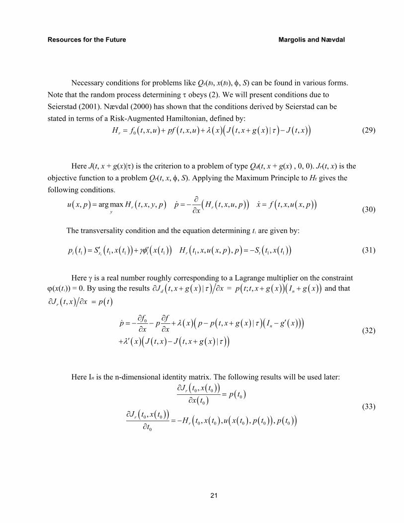
Necessary conditions for problems like Qs(t0, x(t0), φ, S) can be found in various forms. Note that the random process determining τ obeys (2). We will present conditions due to Seierstad (2001). Nævdal (2000) has shown that the conditions derived by Seierstad can be stated in terms of a Risk-Augmented Hamiltonian, defined by:

( ) ( ) ( ) ( )( ) ( )( )0 , , , , , | ,rH f t x u pf t x u x J t x g x J t xλ τ= + + + − (29)

Here J(t, x + g(x)|τ) is the criterion to a problem of type Qd(t, x + g(x) , 0, 0). Jr(t, x) is the objective function to a problem Qr(t, x, φ, S). Applying the Maximum Principle to Hr gives the following conditions.

( ) ( ) ( )( ) ( )( ), arg max , , , , , , , , ,r ry

u x p H t x y p p H t x u p x f t x u x px∂

= = − =∂ (30)

The transversality condition and the equation determining t1 are given by:

( ) ( )( ) ( )( ) ( )( ) ( )( )1 1 1 1 1 1, , , , ,ii x i r t 1,p t S t x t x t H t x u x p p S t x tγφ′ ′= + = − (31)

Here γ is a real number roughly corresponding to a Lagrange multiplier on the constraint ϕ(x(t1)) = 0. By using the results ( )( ), |dJ t x g x xτ∂ + ∂ = ( )( ) ( )(; , n )p t t x g x I g x+ + and that

( ),rJ t x x∂ ∂ ( )p t=

( ) ( )( ) ( )( )( )

( ) ( ) ( )( )( )

0 , |

, , |

nf fp p x p p t x g x I g xx x

x J t x J t x g x

λ τ

λ τ

∂ ∂ ′= − − + − + −∂ ∂

′+ − + (32)

Here In is the n-dimensional identity matrix. The following results will be used later:

( )( )( ) ( )

( )( ) ( ) ( ) ( )( ) ( )( )

0 00

0

0 00 0 0 0 0

0

,

,, , , ,

r

rr

J t x tp t

x t

J t x tH t x t u x t p t p t

t

∂=

∂

∂= −

∂

(33)

21


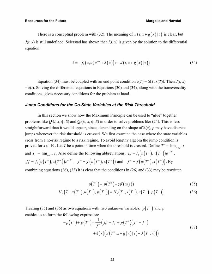
There is a conceptual problem with (32). The meaning of ( )( ),J t x g x |τ+ is clear, but

J(t, x) is still undefined. Seierstad has shown that J(t, x) is given by the solution to the differential equation:

( ) ( ) ( )( )( )0 , ,rtz f x u e x z J t x g x−= − + − + |λ τ (34)

Equation (34) must be coupled with an end point condition z(T) = S(T, x(T)). Then J(t, x) = z(t). Solving the differential equations in Equations (30) and (34), along with the transversality conditions, gives necessary conditions for the problem at hand.

Jump Conditions for the Co-State Variables at the Risk Threshold

In this section we show how the Maximum Principle can be used to “glue” together problems like Qr(t, x, φ, S) and Qs(t0, x, φ, S) in order to solve problems like (24). This is less straightforward than it would appear, since, depending on the shape of λ(x), p may have discrete jumps whenever the risk threshold is crossed. We first examine the case where the state variables cross from a no-risk regime to a risk regime. To avoid lengthy algebra the jump condition is proved for x ∈ . Let T be a point in time when the threshold is crossed. Define T = li

and T = l . Also define the following abbreviations:

R

t Tt+

− mt T

t−→

+ im→ 0f

− = ( ) ( )( )0 , rTf u T x eT−− − − ,

( ) , ( )( ) rT0 0f f u T x+ + T e

++ −= , ( ) ( )( ),f f u T x T+ += + and ( ) ( )( )T,f f u T x− − −= . By

combining equations (26), (33) it is clear that the conditions in (26) and (33) may be rewritten

( ) ( ) ( )( )p T p T x tγφ− + ′= + (35)

( ) ( ) ( )( ) ( ) ( ) ( )( ), , , , , ,d rH T x T u T p T H T x T u T p T− − − − − − − −= (36)

Treating (35) and (36) as two equations with two unknown variables, ( )p T − and γ, enables us to form the following expression:

( ) ( ) ( )( )(

( ) ( )( ) (( ))0 0

1

, | ,

p T p T f f p T f ff

)x J T x g x J T xλ τ

+ − + − + + −−

+ +

− + = − + −

+ + − (37)

22


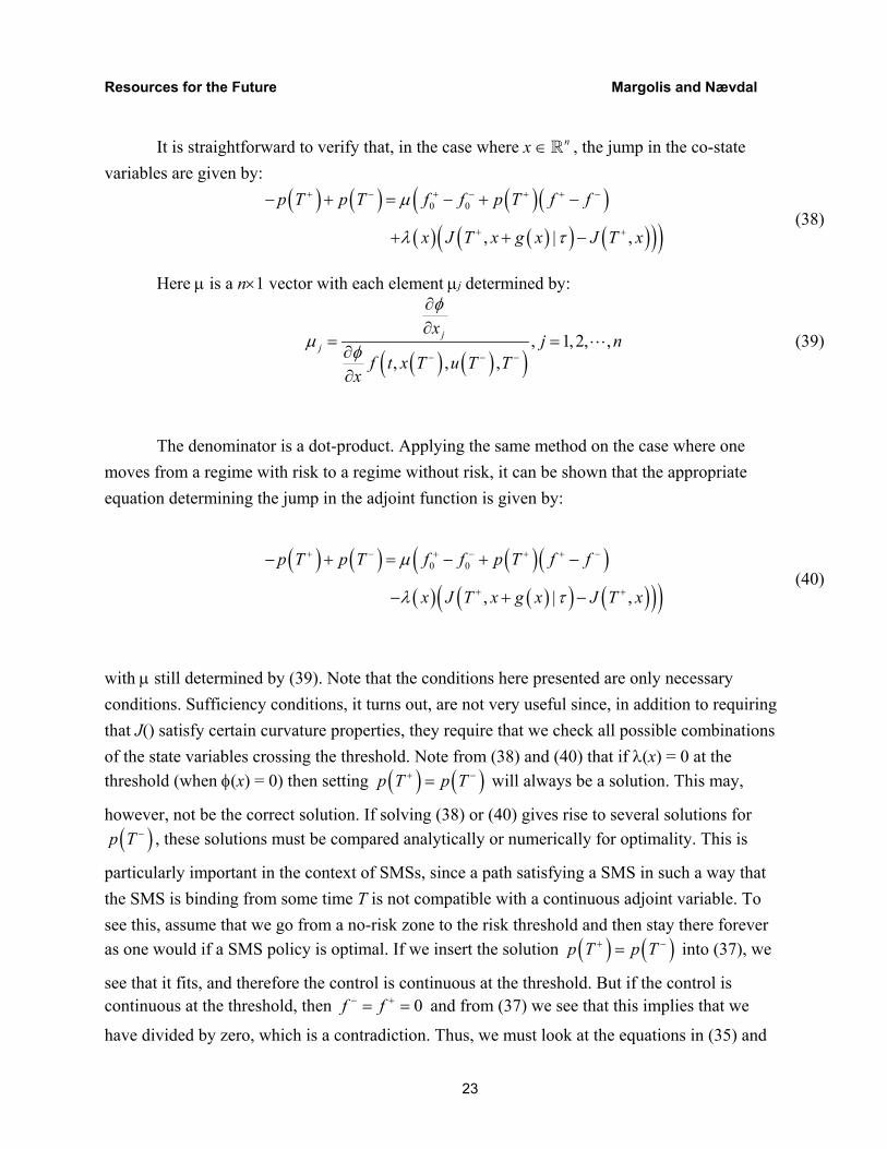
It is straightforward to verify that, in the case where x Rn∈ , the jump in the co-state variables are given by:

( ) ( ) ( )( )(

( ) ( )( ) (( ))0 0

, | ,

p T p T f f p T f f

)x J T x g x J T x

µ

λ τ

+ − + − + + −

+ +

− + = − + −

+ + − (38)

Here µ is a n×1 vector with each element µj determined by:

( ) ( )( )

, 1, 2, ,, , ,

jj

xj

f t x T u T Tx

n

φ

µ φ − − −

∂∂

=∂∂

= (39)

The denominator is a dot-product. Applying the same method on the case where one moves from a regime with risk to a regime without risk, it can be shown that the appropriate equation determining the jump in the adjoint function is given by:

( ) ( ) ( )( )(

( ) ( )( ) (( ))0 0

, | ,

p T p T f f p T f f

)x J T x g x J T x

µ

λ τ

+ − + − + + −

+ +

− + = − + −

− + − (40)

with µ still determined by (39). Note that the conditions here presented are only necessary conditions. Sufficiency conditions, it turns out, are not very useful since, in addition to requiring that J() satisfy certain curvature properties, they require that we check all possible combinations of the state variables crossing the threshold. Note from (38) and (40) that if λ(x) = 0 at the threshold (when φ(x) = 0) then setting ( ) ( )p T p T+ −= will always be a solution. This may,

however, not be the correct solution. If solving (38) or (40) gives rise to several solutions for ( )p T − , these solutions must be compared analytically or numerically for optimality. This is

particularly important in the context of SMSs, since a path satisfying a SMS in such a way that the SMS is binding from some time T is not compatible with a continuous adjoint variable. To see this, assume that we go from a no-risk zone to the risk threshold and then stay there forever as one would if a SMS policy is optimal. If we insert the solution ( ) ( )p T p T+ −= into (37), we

see that it fits, and therefore the control is continuous at the threshold. But if the control is continuous at the threshold, then 0f f− += = and from (37) we see that this implies that we

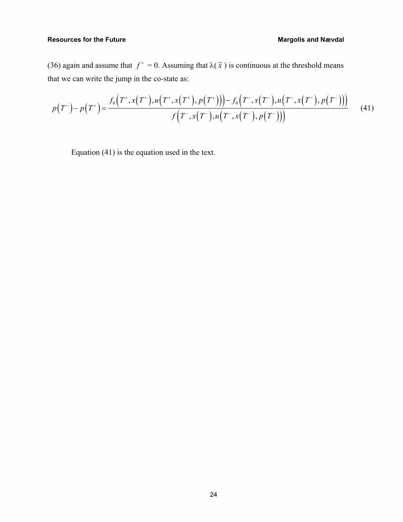
have divided by zero, which is a contradiction. Thus, we must look at the equations in (35) and

23


(36) again and assume that f + = 0. Assuming that λ( x ) is continuous at the threshold means

that we can write the jump in the co-state as:

)( )( )x T+ +

( ) ( )( ) ( ) ( ( ) ( ) ( )( )( )

( ) ( ) ( )( )( )0 0, , , , , , , ,

, , , ,

f T u T x T p T f T x T u T x T p Tp T p T

f T x T u T x T p T

+ + + − − − − −

− +

− − − − −

−− = (41)

Equation (41) is the equation used in the text.

24


References

Bishop, R. C. 1978. Endangered Species and Uncertainty: The Economics of a Safe Minimum Standard. American Journal of Agricultural Economics 60(1): 10–18.

———. 1979. Endangered Species, Irreversibility, and Uncertainty: A Reply. American Journal of Agricultural Economics 61(2): 376–379.

Boyle, K. J., and R. C. Bishop. 1987. Valuing Wildlife in Benefit-Cost Analyses: A Case Study Involving Endangered Species. Water Resources Research 23(5): 943–50.

Clarke, H. R., and W. J. Reed, 1994. Consumption/pollution tradeoffs in an environment vulnerable to pollution-related catastrophic collapse, Journal of Economic Dynamics and Control, (18) 991 – 1010.

Ciriacy-Wantrup, S.V. 1952. Resource Conservation. Berkeley, CA: University of California Press.

Cropper, M. L. 1976. Regulating Activities with Catastrophic Environmental Effects. Journal of Environmental Economics and Management. (3): 1–15.

Crowards, Tom M. 1998. Safe Minimum Standards: Costs and Opportunities. Ecological Economics 25: 303–314.

Dasgupta, P., and G. Heal.1974. The Optimal Depletion of Exhaustible Resources, Review of Economic Studies, Symposium on the Economics of Exhaustible Resources, 3–28.

25


Dixit , A. K., and R. S. Pindyck. 1994. Investment under Uncertainty. Princeton, NJ: Princeton University Press.

Farmer, M.C. and A. Randall. 1998. The Rationality of a Safe Minimum Standard. Land Economics, 74(3): 287–302.

Heal, G. 1991. Economy and Climate: a Preliminary Framework for Microeconomic Analysis. In R. Just & N. Bockstael (eds.), Commodity and Resource Policies in Agricultural Systems. Berlin, Heidelberg, and New York: Springer, 196–212.

Kemp, M. C. 1976. Three Topics in the Theory of International Trade. Amsterdam: North-Holland Elsvier Science.

Knight, F. 1921. Risk, Uncertainty and Profit. Boston: Houghton-Mifflin.

Mason, C. F. 1996. Biology of Freshwater Pollution. Essex, England: Longman.,

Nævdal, E. 2001. Optimal Regulation of Eutrophying Lakes, Fjords and Rivers in the Presence of Threshold Effects. American Journal of Agricultural Economics 84(4).

———. 2003a. Optimal Regulation of Natural Resources in the Presence of Irreversible Threshold Effects, Natural Resource Modeling. 16, 3:305–333.

———. 2003b. Dynamic Optimization in the Presence of Threshold Effects When the Location of the Threshold is Uncertain—With an Application to a Possible Disintegration of the Western Antarctic Ice Sheet. Woodrow Wilson School Discussion Papers in Economics #224, Princeton University. Available at http://www.wws.princeton.edu/~econdp/pdf/dp224.pdf.

26

http://www.wws.princeton.edu/~econdp/pdf/dp224.pdf


Nævdal, E., and M. Margolis. 2001. Optimal Resource Management with a Safe Minimum Standard - Conditions for Living on the Edge of Risk IØS discussion paper D18/2001, Agricultural University of Norway, Available at http://www.nlh.no/ios/Publikasjoner/d2001/d2001-18.html.

Norton B. G., and M. A. Toman. 1997. Sustainability: Ecological and Economic Perspectives. Land Economics 73(4): 553–568.

Ready, Richard C., and Richard C. Bishop. 1991. Endangered Species and the Safe Minimum Standard. American Journal of Agricultural Economics 72(2): 309–12

Rolfe, J. C. 1995. Ulysses Revisited—A Closer Look at the Safe Minimum Standard. Australian Journal of Agricultural Economics 39(1):55–70.

Samuelson, P. 1947. Foundations of Economic Analysis. Cambridge, MA: Harvard University Press.

Seierstad, A. 2001. Necessary Conditions and Sufficient Conditions for Optimal Control of Piecewise Deterministic Control Systems. Memorandum, Dept. of Economics, University of Oslo.

Seierstad, A., and K. Sydsæter.1987. Optimal Control Theory with Economic Applications. Amsterdam: North-Holland Elsevier Science.

Smith, V. K., and J. V. Krutilla. 1979. Endangered Species, Irreversibilities, and Uncertainty: A Comment. American Journal of Agricultural Economics 61(2): 371–75.

27

http://www.nlh.no/ios/Publikasjoner/d2001/d2001-18.html


Soule, M.E. 1987. Viable Populations for Conservation. Cambridge, MA: Cambridge University Press.

Tsur, Y., and A. Zemel. 1995. Uncertainty and Irreversibility in Groundwater Management, Journal of Environmental Economics and Management, 29, 149–161.

———. 1996. Accounting for Global Warming Risks: Resource Management under Event Uncertainty, Journal of Economic Dynamics and Control, 20, 1289–1305.

Zelikin, M. I., and Borisov V.F. 1994. The Theory of Chattering Control, Boston: Birkhäuser.

28

Safe Minimum Standards in Dynamic Resource Problems

Documents

Transcript of Safe Minimum Standards in Dynamic Resource Problems