Sabur Ajibola Alim and Nahrul Khair Alang Rashid

Chapter 1

Some Commonly Used Speech Feature ExtractionAlgorithms

Sabur Ajibola Alim and Nahrul Khair Alang Rashid

Additional information is available at the end of the chapter

http://dx.doi.org/10.5772/intechopen.80419

Provisional chapter

Some Commonly Used Speech Feature ExtractionAlgorithms

Sabur Ajibola Alim and Nahrul Khair Alang Rashid

Additional information is available at the end of the chapter

Abstract

Speech is a complex naturally acquired human motor ability. It is characterized in adultswith the production of about 14 different sounds per second via the harmonized actions ofroughly 100 muscles. Speaker recognition is the capability of a software or hardware toreceive speech signal, identify the speaker present in the speech signal and recognize thespeaker afterwards. Feature extraction is accomplished by changing the speech waveformto a form of parametric representation at a relatively minimized data rate for subsequentprocessing and analysis. Therefore, acceptable classification is derived from excellent andquality features. Mel Frequency Cepstral Coefficients (MFCC), Linear Prediction Coeffi-cients (LPC), Linear Prediction Cepstral Coefficients (LPCC), Line Spectral Frequencies(LSF), Discrete Wavelet Transform (DWT) and Perceptual Linear Prediction (PLP) are thespeech feature extraction techniques that were discussed in these chapter. These methodshave been tested in a wide variety of applications, giving them high level of reliability andacceptability. Researchers have made several modifications to the above discussed tech-niques to make them less susceptible to noise, more robust and consume less time. Inconclusion, none of the methods is superior to the other, the area of application woulddetermine which method to select.

Keywords: human speech, speech features, mel frequency cepstral coefficients (MFCC),linear prediction coefficients (LPC), linear prediction cepstral coefficients (LPCC), linespectral frequencies (LSF), discrete wavelet transform (DWT), perceptual linear prediction(PLP)

1. Introduction

Human beings express their feelings, opinions, views and notions orally through speech. Thespeech production process includes articulation, voice, and fluency [1, 2]. It is a complex

© 2016 The Author(s). Licensee InTech. This chapter is distributed under the terms of the Creative Commons

Attribution License (http://creativecommons.org/licenses/by/3.0), which permits unrestricted use,

distribution, and eproduction in any medium, provided the original work is properly cited.

DOI: 10.5772/intechopen.80419

© 2018 The Author(s). Licensee IntechOpen. This chapter is distributed under the terms of the CreativeCommons Attribution License (http://creativecommons.org/licenses/by/3.0), which permits unrestricted use,distribution, and reproduction in any medium, provided the original work is properly cited.

naturally acquired human motor abilities, a task categorized in regular adults by the productionof about 14 different sounds per second via the harmonized actions of roughly 100 musclesconnected by spinal and cranial nerves. The simplicity with which human beings speak is incontrast to the complexity of the task, and that complexity could assist in explaining why speechcan be very sensitive to diseases associated with the nervous system [3].

There have been several successful attempts in the development of systems that can analyze,classify and recognize speech signals. Both hardware and software that have been developedfor such tasks have been applied in various fields such as health care, government sectors andagriculture. Speaker recognition is the capability of a software or hardware to receive speechsignal, identify the speaker present in the speech signal and recognize the speaker afterwards [4].Speaker recognition executes a task similar to what the human brain undertakes. This startsfrom speech which is an input to the speaker recognition system. Generally, speaker recogni-tion process takes place in three main steps which are acoustic processing, feature extractionand classification/recognition [5].

The speech signal has to be processed to remove noise before the extraction of the importantattributes in the speech [6] and identification. The purpose of feature extraction is to illustrate aspeech signal by a predetermined number of components of the signal. This is because all theinformation in the acoustic signal is too cumbersome to deal with, and some of the informationis irrelevant in the identification task [7, 8].

Feature extraction is accomplished by changing the speech waveform to a form of parametricrepresentation at a relatively lesser data rate for subsequent processing and analysis. This isusually called the front end signal-processing [9, 10]. It transforms the processed speech signalto a concise but logical representation that is more discriminative and reliable than the actualsignal. With front end being the initial element in the sequence, the quality of the subsequentfeatures (pattern matching and speaker modeling) is significantly affected by the quality of thefront end [10].

Therefore, acceptable classification is derived from excellent and quality features. In presentautomatic speaker recognition (ASR) systems, the procedure for feature extraction has nor-mally been to discover a representation that is comparatively reliable for several conditions ofthe same speech signal, even with alterations in the environmental conditions or speaker,while retaining the portion that characterizes the information in the speech signal [7, 8].

Feature extraction approaches usually yield a multidimensional feature vector for everyspeech signal [11]. A wide range of options are available to parametrically represent the speechsignal for the recognition process, such as perceptual linear prediction (PLP), linear predictioncoding (LPC) and mel-frequency cepstrum coefficients (MFCC). MFCC is the best known andvery popular [9, 12]. Feature extraction is the most relevant portion of speaker recognition.Features of speech have a vital part in the segregation of a speaker from others [13]. Featureextraction reduces the magnitude of the speech signal devoid of causing any damage to thepower of speech signal [14].

Before the features are extracted, there are sequences of preprocessing phases that are firstcarried out. The preprocessing step is pre-emphasis. This is achieved by passing the signal

From Natural to Artificial Intelligence - Algorithms and Applications4

through a FIR filter [15] which is usually a first-order finite impulse response (FIR) filter [16].This is succeeded by frame blocking, a method of partitioning the speech signal into frames. Itremoves the acoustic interface existing in the start and end of the speech signal [17].

The framed speech signal is then windowed. Bandpass filter is a suitable window [15] that isapplied to minimize disjointedness at the start and finish of each frame. The two most famouscategories of windows are Hamming and Rectangular windows [18]. It increases the sharpnessof harmonics, eliminates the discontinuous of signal by tapering beginning and ending of theframe zero. It also reduces the spectral distortion formed by the overlap [17].

2. Mel frequency cepstral coefficients (MFCC)

Mel frequency cepstral coefficients (MFCC) was originally suggested for identifying monosyl-labic words in continuously spoken sentences but not for speaker identification. MFCC com-putation is a replication of the human hearing system intending to artificially implement theear’s working principle with the assumption that the human ear is a reliable speaker recog-nizer [19]. MFCC features are rooted in the recognized discrepancy of the human ear’s criticalbandwidths with frequency filters spaced linearly at low frequencies and logarithmically athigh frequencies have been used to retain the phonetically vital properties of the speech signal.Speech signals commonly contain tones of varying frequencies, each tone with an actualfrequency, f (Hz) and the subjective pitch is computed on the Mel scale. The mel-frequencyscale has linear frequency spacing below 1000 Hz and logarithmic spacing above 1000 Hz.Pitch of 1 kHz tone and 40 dB above the perceptual audible threshold is defined as 1000 mels,and used as reference point [20].

MFCC is based on signal disintegration with the help of a filter bank. The MFCC gives adiscrete cosine transform (DCT) of a real logarithm of the short-term energy displayed on theMel frequency scale [21]. MFCC is used to identify airline reservation, numbers spoken into atelephone and voice recognition system for security purpose. Some modifications have beenproposed to the basic MFCC algorithm for better robustness, such as by lifting the log-mel-amplitudes to an appropriate power (around 2 or 3) before applying the DCTand reducing theimpact of the low-energy parts [4].

2.1. Algorithm description, strength and weaknesses

MFCC are cepstral coefficients derived on a twisted frequency scale centerd on human audi-tory perception. In the computation of MFCC, the first thing is windowing the speech signal tosplit the speech signal into frames. Since the high frequency formants process reduced ampli-tude compared to the low frequency formants, high frequencies are emphasized to obtainsimilar amplitude for all the formants. After windowing, Fast Fourier Transform (FFT) isapplied to find the power spectrum of each frame. Subsequently, the filter bank processing iscarried out on the power spectrum, using mel-scale. The DCT is applied to the speech signal

Some Commonly Used Speech Feature Extraction Algorithmshttp://dx.doi.org/10.5772/intechopen.80419

5

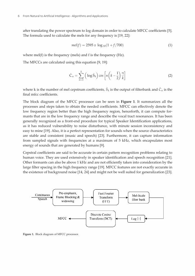
after translating the power spectrum to log domain in order to calculate MFCC coefficients [5].The formula used to calculate the mels for any frequency is [19, 22]:

mel fð Þ ¼ 2595 x log 10 1þ f =700ð Þ (1)

where mel(f) is the frequency (mels) and f is the frequency (Hz).

The MFCCs are calculated using this equation [9, 19]:

Cn ¼Xk

n¼1

log Sk

� �cos n k� 1

2

� �πk

� �(2)

where k is the number of mel cepstrum coefficients, Sk is the output of filterbank and Cn is thefinal mfcc coefficients.

The block diagram of the MFCC processor can be seen in Figure 1. It summarizes all theprocesses and steps taken to obtain the needed coefficients. MFCC can effectively denote thelow frequency region better than the high frequency region, henceforth, it can compute for-mants that are in the low frequency range and describe the vocal tract resonances. It has beengenerally recognized as a front-end procedure for typical Speaker Identification applications,as it has reduced vulnerability to noise disturbance, with minute session inconsistency andeasy to mine [19]. Also, it is a perfect representation for sounds when the source characteristicsare stable and consistent (music and speech) [23]. Furthermore, it can capture informationfrom sampled signals with frequencies at a maximum of 5 kHz, which encapsulates mostenergy of sounds that are generated by humans [9].

Cepstral coefficients are said to be accurate in certain pattern recognition problems relating tohuman voice. They are used extensively in speaker identification and speech recognition [21].Other formants can also be above 1 kHz and are not efficiently taken into consideration by thelarge filter spacing in the high frequency range [19]. MFCC features are not exactly accurate inthe existence of background noise [14, 24] and might not be well suited for generalization [23].

Figure 1. Block diagram of MFCC processor.


3. Linear prediction coefficients (LPC)

Linear prediction coefficients (LPC) imitates the human vocal tract [16] and gives robustspeech feature. It evaluates the speech signal by approximating the formants, getting rid of itseffects from the speech signal and estimate the concentration and frequency of the left behindresidue. The result states each sample of the signal as a direct incorporation of previoussamples. The coefficients of the difference equation characterize the formants, thus, LPC needsto approximate these coefficients [25]. LPC is a powerful speech analysis method and it hasgained fame as a formant estimation method [17].

The frequencies where the resonant crests happen are called the formant frequencies. Thus,with this technique, the positions of the formants in a speech signal are predictable by calcu-lating the linear predictive coefficients above a sliding window and finding the crests in thespectrum of the subsequent linear prediction filter [17]. LPC is helpful in the encoding of highquality speech at low bit rate [13, 26, 27].

Other features that can be deduced from LPC are linear predication cepstral coefficients(LPCC), log area ratio (LAR), reflection coefficients (RC), line spectral frequencies (LSF) andArcus Sine Coefficients (ARCSIN) [13]. LPC is generally used for speech reconstruction. LPCmethod is generally applied in musical and electrical firms for creating mobile robots, intelephone firms, tonal analysis of violins and other string musical gadgets [4].


Linear prediction method is applied to obtain the filter coefficients equivalent to the vocal tractby reducing the mean square error in between the input speech and estimated speech [28].Linear prediction analysis of speech signal forecasts any given speech sample at a specificperiod as a linear weighted aggregation of preceding samples. The linear predictive model ofspeech creation is given as [13, 25]:

s nð Þ ¼Xpk¼1

aks n� kð Þ (3)

where s is the predicted sample, s is the speech sample, p is the predictor coefficients.

The prediction error is given as [16, 25]:

e nð Þ ¼ s nð Þ � s nð Þ (4)

Subsequently, each frame of the windowed signal is autocorrelated, while the highest autocor-relation value is the order of the linear prediction analysis. This is followed by the LPCanalysis, where each frame of the autocorrelations is converted into LPC parameters set whichconsists of the LPC coefficients [26]. A summary of the procedure for obtaining the LPC is asseen in Figure 2. LPC can be derived by [7]:


7

am ¼ log1� km1þ km

� �(5)

where am is the linear prediction coefficient, km is the reflection coefficient.

Linear predictive analysis efficiently selects the vocal tract information from a given speech[16]. It is known for the speed of computation and accuracy [18]. LPC excellently represents thesource behaviors that are steady and consistent [23]. Furthermore, it is also be used in speakerrecognition system where the main purpose is to extract the vocal tract properties [25]. It givesvery accurate estimates of speech parameters and is comparatively efficient for computation[14, 26]. Traditional linear prediction suffers from aliased autocorrelation coefficients [29]. LPCestimates have high sensitivity to quantization noise [30] and might not be well suited forgeneralization [23].

4. Linear prediction cepstral coefficients (LPCC)

Linear prediction cepstral coefficients (LPCC) are cepstral coefficients derived from LPC cal-culated spectral envelope [11]. LPCC are the coefficients of the Fourier transform illustration ofthe logarithmic magnitude spectrum [30, 31] of LPC. Cepstral analysis is commonly applied inthe field of speech processing because of its ability to perfectly symbolize speech waveformsand characteristics with a limited size of features [31].

It was observed by Rosenberg and Sambur that adjacent predictor coefficients are highlycorrelated and therefore, representations with less correlated features would be more efficient,LPCC is a typical example of such. The relationship between LPC and LPCC was originallyderived by Atal in 1974. In theory, it is relatively easy to convert LPC to LPCC, in the case ofminimum phase signals [32].


In speech processing, LPCC analogous to LPC, are computed from sample points of a speechwaveform, the horizontal axis is the time axis, while the vertical axis is the amplitude axis [31].

Figure 2. Block diagram of LPC processor.


The LPCC processor is as seen in Figure 3. It pictorially explains the process of obtainingLPCC. LPCC can be calculated using [7, 15, 33]:

Cm ¼ am þXm�1

k¼1

km

� �ckam�k (6)

where am is the linear prediction coefficient, Cm is the cepstral coefficient.

LPCC have low vulnerability to noise [30]. LPCC features yield lower error rate as comparedto LPC features [31]. Cepstral coefficients of higher order are mathematically limited, resultingin an extremely extensive array of variances when moving from the cepstral coefficients oflower order to cepstral coefficients of higher order [34]. Similarly, LPCC estimates are notori-ous for having great sensitivity to quantization noise [35]. Cepstral analysis on high-pitchspeech signal gives small source-filter separability in the quefrency domain [29]. Cepstralcoefficients of lower order are sensitive to the spectral slope, while the cepstral coefficients ofhigher order are sensitive to noise [15].

5. Line spectral frequencies (LSF)

Individual lines of the Line Spectral Pairs (LSP) are known as line spectral frequencies (LSF).LSF defines the two resonance situations taking place in the inter-connected tube model of thehuman vocal tract. The model takes into consideration the nasal cavity and the mouth shape,which gives the basis for the fundamental physiological importance of the linear predictionillustration. The two resonance situations define the vocal tract as either being completely openor completely closed at the glottis [36]. The two situations begets two groups of resonantfrequencies, with the number of resonances in each group being deduced from the quantity oflinked tubes. The resonances of each situation are the odd and even line spectra correspond-ingly, and are interwoven into a singularly rising group of LSF [36].

The LSF representation was proposed by Itakura [37, 38] as a substitute to the linear predictionparametric illustration. In the area of speech coding, it has been realized that this illustrationhas an improved quantization features than the other linear prediction parametric illustrations

Figure 3. Block diagram of LPCC processor.


9

(LAR and RC). The LSF illustration has the capacity to reduce the bit-rate by 25–30% fortransmitting the linear prediction information without distorting the quality of synthesizedspeech [38–40]. Apart from quantization, LSF illustration of the predictor are also suitable forinterpolation. Theoretically, this can be inspired by the point that the sensitivity matrix linkingthe LSF-domain squared quantization error to the perceptually relevant log spectrum is diag-onal [41, 42].


LP is established on the point that a speech signal can be defined by Eq. (3). Recall

s nð Þ ¼Xpk¼1

aks n� kð Þ

where k is the time index and p is the order of the linear prediction, s nð Þ is the predictor signaland ak is the LPC coefficients.

The ak coefficients are determined in order to reduce the prediction error by method ofautocorrelation or covariance. Eq. (3) can be modified in the frequency domain with the z-transform. As such, a small part of the speech signal is anticipated to be given as an output tothe all-pole filter H zð Þ. The new equation is

H zð Þ ¼ 1A zð Þ ¼

11�Pp

i¼1 aiz�1(7)

where H zð Þ is the all-pole filter and A zð Þ is the LPC analysis filter.

In order to compute the LSF coefficients, an inverse polynomial filter is split into two poly-nomials P zð Þ and Q zð Þ [36, 38, 40, 41]:

P zð Þ ¼ A zð Þ þ z� pþ1ð ÞA z�1� (8)

Q zð Þ ¼ A zð Þ � z� pþ1ð ÞA z�1� (9)

where P zð Þ is the vocal tract with the glottis closed, Q zð Þ is the LPC analysis filter of order p.

In order to convert LSF back to LPC, the equation below is used [36, 41, 43, 44]:

A zð Þ ¼ 0:5 P zð Þ þQ zð Þ½ � (10)

The block diagram of the LSF processor is as seen in Figure 4. The most prominent applicationof LSF is in the area of speech compression, with extension into the speaker recognition andspeech recognition. This technique has also found restricted use in other fields. LSF have beeninvestigated for use in musical instrument recognition and coding. LSF have also been appliedto animal noise identification, recognizing individual instruments and financial market analy-sis. The advantages of LSF include their ability to localize spectral sensitivities, the fact that


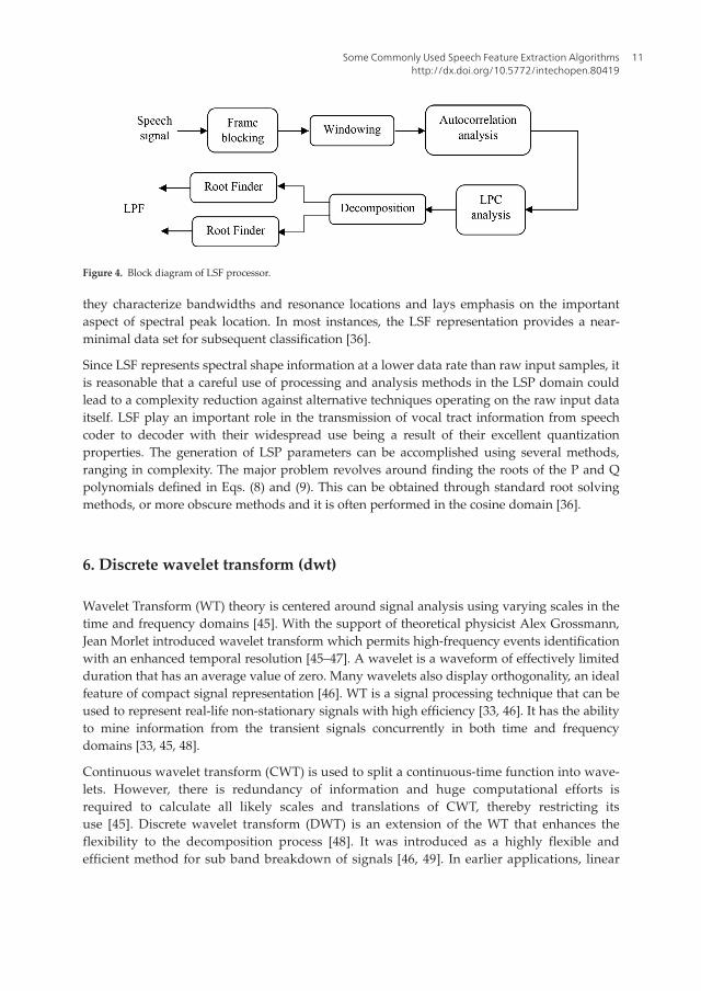
they characterize bandwidths and resonance locations and lays emphasis on the importantaspect of spectral peak location. In most instances, the LSF representation provides a near-minimal data set for subsequent classification [36].

Since LSF represents spectral shape information at a lower data rate than raw input samples, itis reasonable that a careful use of processing and analysis methods in the LSP domain couldlead to a complexity reduction against alternative techniques operating on the raw input dataitself. LSF play an important role in the transmission of vocal tract information from speechcoder to decoder with their widespread use being a result of their excellent quantizationproperties. The generation of LSP parameters can be accomplished using several methods,ranging in complexity. The major problem revolves around finding the roots of the P and Qpolynomials defined in Eqs. (8) and (9). This can be obtained through standard root solvingmethods, or more obscure methods and it is often performed in the cosine domain [36].

6. Discrete wavelet transform (dwt)

Wavelet Transform (WT) theory is centered around signal analysis using varying scales in thetime and frequency domains [45]. With the support of theoretical physicist Alex Grossmann,Jean Morlet introduced wavelet transform which permits high-frequency events identificationwith an enhanced temporal resolution [45–47]. A wavelet is a waveform of effectively limitedduration that has an average value of zero. Many wavelets also display orthogonality, an idealfeature of compact signal representation [46]. WT is a signal processing technique that can beused to represent real-life non-stationary signals with high efficiency [33, 46]. It has the abilityto mine information from the transient signals concurrently in both time and frequencydomains [33, 45, 48].

Continuous wavelet transform (CWT) is used to split a continuous-time function into wave-lets. However, there is redundancy of information and huge computational efforts isrequired to calculate all likely scales and translations of CWT, thereby restricting itsuse [45]. Discrete wavelet transform (DWT) is an extension of the WT that enhances theflexibility to the decomposition process [48]. It was introduced as a highly flexible andefficient method for sub band breakdown of signals [46, 49]. In earlier applications, linear

Figure 4. Block diagram of LSF processor.


11

discretization was used for discretizing CWT. Daubechies and others have developed anorthogonal DWT specially designed for analyzing a finite set of observations over the set ofscales (dyadic discretization) [47].


Wavelet transform decomposes a signal into a group of basic functions called wavelets. Wave-lets are obtained from a single prototype wavelet called mother wavelet by dilations andshifting. The main characteristic of the WT is that it uses a variable window to scan thefrequency spectrum, increasing the temporal resolution of the analysis [45, 46, 50].

WTdecomposes signals over translated and dilated mother wavelets. Mother wavelet is a timefunction with finite energy and fast decay. The different versions of the single wavelet areorthogonal to each other. The continuous wavelet transform (CWT) is given by [33, 45, 50]:

Wx a; bð Þ ¼ 1ffiffiffia

pð∞

�∞

x tð Þψ∗ t� ba

� �dt (11)

where ψ tð Þ is the mother wavelet, a and b are continuous parameters.

The WT coefficient is an expansion and a particular shift represents how well the original signalcorresponds to the translated and dilated mother wavelet. Thus, the coefficient group of CWT(a, b) associated with a particular signal is the wavelet representation of the original signal inrelation to the mother wavelet [45]. Since CWT contains high redundancy, analyzing the signalusing a small number of scales with varying number of translations at each scale, i.e. discretizingscale and translation parameters as a ¼ 2j and b ¼ 2jk gives DWT. DWT theory requires two setsof related functions called scaling function and wavelet function given by [33]:

ϕ tð Þ ¼XN�1

n¼0

h n½ �ffiffiffi2

pϕ 2t� nð Þ (12)

ψ tð Þ ¼XN�1

n¼0

g n½ �ffiffiffi2

pϕ 2t� nð Þ (13)

where ϕ tð Þ is the scaling function, ψ tð Þ is the wavelet function, h[n] is the an impulse responseof a low-pass filter, and g[n] is an impulse response of a high-pass filter.

There are several ways to discretize a CWT. The DWT of the continuous signal can also begiven by [45]:

DWTð Þ m; pð Þ ¼ðþ∞

�∞

x tð Þ∙ψm,pdt (14)

where ψm,p is the wavelet function bases, m is the dilation parameter and p is the translation

parameter.


Thus, ψm,p is defined as:

ψm,p ¼1ffiffiffiffiffiam0

p ψt� pb0am0

am0

� �(15)

The DWT of a discrete signal is derived from CWT and defined as:

DWTð Þ m; kð Þ ¼ 1ffiffiffiffiffiam0

p Xn

x n½ �∙g n� nb0am0am0

� �(16)

where g(*) is the mother wavelet and x[n] is the discretized signal. The mother wavelet may bedilated and translated discretely by selecting the scaling parameter a ¼ am0 and translationparameter b ¼ nb0am0 (with constants taken as a0 > 1, b0 > 1, while m and n are assigned a setof positive integers).

The scaling and wavelet functions can be implemented effectively using a pair of filters, h[n]

and g[n], called quadrature mirror filters that confirm with the property g n½ � ¼ �1ð Þ1�nh n½ �.The input signal is filtered by a low-pass filter and high-pass filter to obtain the approximatecomponents and the detail components respectively. This is summarized in Figure 5. Theapproximate signal at each stage is further decomposed using the same low-pass and high-pass filters to get the approximate and detail components for the next stage. This type ofdecomposition is called dyadic decomposition [33].

The DWT parameters contain the information of different frequency scales. This enhancesthe speech information obtained in the corresponding frequency band [33]. The ability of theDWT to partition the variance of the elements of the input on a scale by scale basis is anadded advantage. This partitioning leads to the opinion of the scale-dependent waveletvariance, which in many ways is equivalent to the more familiar frequency-dependentFourier power spectrum [47]. Classic discrete decomposition schemes, which are dyadic donot fulfill all the requirements for direct use in parameterization. DWT does provide ade-quate number of frequency bands for effective speech analysis [51]. Since the input signalsare of finite length, the wavelet coefficients will have unwantedly large variations at theboundaries because of the discontinuities at the boundaries [50].

Figure 5. Block diagram of DWT.


13

7. Perceptual linear prediction (PLP)

Perceptual linear prediction (PLP) technique combines the critical bands, intensity-to-loudnesscompression and equal loudness pre-emphasis in the extraction of relevant information fromspeech. It is rooted in the nonlinear bark scale and was initially intended for use in speechrecognition tasks by eliminating the speaker dependent features [11]. PLP gives a representa-tion conforming to a smoothed short-term spectrum that has been equalized and compressedsimilar to the human hearing making it similar to the MFCC. In the PLP approach, severalprominent features of hearing are replicated and the consequent auditory like spectrum ofspeech is approximated by an autoregressive all–pole model [52]. PLP gives minimized reso-lution at high frequencies that signifies auditory filter bank based approach, yet gives theorthogonal outputs that are similar to the cepstral analysis. It uses linear predictions forspectral smoothing, hence, the name is perceptual linear prediction [28]. PLP is a combinationof both spectral analysis and linear prediction analysis.


In order to compute the PLP features the speech is windowed (Hamming window), the FastFourier Transform (FFT) and the square of the magnitude are computed. This gives the powerspectral estimates. A trapezoidal filter is then applied at 1-bark interval to integrate theoverlapping critical band filter responses in the power spectrum. This effectively compressesthe higher frequencies into a narrow band. The symmetric frequency domain convolution onthe bark warped frequency scale then permits low frequencies to mask the high frequencies,concurrently smoothing the spectrum. The spectrum is subsequently pre-emphasized to approx-imate the uneven sensitivity of human hearing at a variety of frequencies. The spectral ampli-tude is compressed, this reduces the amplitude variation of the spectral resonances. An InverseDiscrete Fourier Transform (IDCT) is performed to get the autocorrelation coefficients. Spec-tral smoothing is performed, solving the autoregressive equations. The autoregressive coeffi-cients are converted to cepstral variables [28]. The equation for computing the bark scalefrequency is:

Figure 6. Block diagram of PLP processor.


Typeof

Filter

Shap

eof

filter

What

ismod

eled

Speedof

computation

Typeof

coefficien

tNoise

resistan

ceSen

sitivity

toquan

tization

/additional

noise

Reliability

Freq

uen

cycaptured

Mel

freq

uenc

yceps

tral

coeffic

ient

(MFC

C)

Mel

Triang

ular

Hum

anAud

itory

System

High

Cep

stral

Med

ium

Med

ium

High

Low

Line

arpred

ictio

ncoeffic

ient

(LPC

)Line

arPred

ictio

nLine

arHum

anVocal

Tract

High

Autocorrelatio

nCoe

fficient

High

High

High

Low

Line

arpred

ictio

nceps

tral

coeffic

ient

(LPC

C)

Line

arPred

ictio

nLine

arHum

anVocal

Tract

Med

ium

Cep

stral

High

High

Med

ium

Low

&Med

ium

Line

spectral

freq

uenc

ies

(LSF

)Line

arPred

ictio

nLine

arHum

anVocal

Tract

Med

ium

Spectral

High

High

Med

ium

Low

&Med

ium

Discretewav

elet

tran

sform

(DWT)

Lowpa

ss&

high

pass

——

High

Wav

elets

Med

ium

Med

ium

Med

ium

Low

&High

Percep

tual

linear

pred

ictio

n(PLP)

Bark

Trap

ezoida

lHum

anAud

itory

System

Med

ium

Cep

stral&

Autocorrelatio

nMed

ium

Med

ium

Med

ium

Low

&Med

ium

Table

1.Com

parisonbe

tweenthefeatureextractio

ntech

niqu

es.


15

bark fð Þ ¼ 26:81 f1960þ f

� 0:53 (17)

where bark(f) is the frequency (bark) and f is the frequency (Hz).

The identification achieved by PLP is better than that of LPC [28], because it is an improvementover the conventional LPC because it effectively suppresses the speaker-dependent informa-tion [52]. Also, it has enhanced speaker independent recognition performance and is robust tonoise, variations in the channel and microphones [53]. PLP reconstructs the autoregressivenoise component accurately [54]. PLP based front end is sensitive to any change in the formantfrequency.

Figure 6 shows the PLP processor, showing all the steps to be taken to obtain the PLPcoefficients. PLP has low sensitivity to spectral tilt, consistent with the findings that it isrelatively insensitive to phonetic judgments of the spectral tilt. Also, PLP analysis is dependenton the result of the overall spectral balance (formant amplitudes). The formant amplitudes areeasily affected by factors such as the recording equipment, communication channel and addi-tive noise [52]. Furthermore, the time-frequency resolution and efficient sampling of the short-term representation are addressed in an ad-hoc way [54].

Table 1 shows a comparison between the six feature extraction techniques that have beenexplicitly described above. Even though the selection of a feature extraction algorithm for usein research is individual dependent, however, this table has been able to characterize thesetechniques based on the main considerations in the selection of any feature extraction algo-rithm. The considerations include speed of computation, noise resistance and sensitivity toadditional noise. The table also serves as a guide when considering the selection between anytwo or more of the discussed algorithms.

8. Conclusion

MFCC, LPC, LPCC, LSF, PLP and DWT are some of the feature extraction techniques used forextracting relevant information form speech signals for the purpose speech recognition andidentification. These techniques have stood the test of time and have been widely used inspeech recognition systems for several purposes. Speech signal is a slow time varying signal,quasi-stationary, when observed over an adequately short period of time between 5 and100 msec, its behavior is relatively stationary. As a result of this, short time spectral analysiswhich includes MFCC, LPCC and PLP are commonly used for the extraction of importantinformation from speech signals. Noise is a serious challenge encountered in the process offeature extraction, as well as speaker recognition as a whole. Subsequently, researchers havemade several modifications to the above discussed techniques to make them less susceptible tonoise, more robust and consume less time. These methods have also been used in the recogni-tion of sounds. The extracted information will be the input to the classifier for identificationpurposes. The above discussed feature extraction approaches can be implemented usingMATLAB.


Author details

Sabur Ajibola Alim1* and Nahrul Khair Alang Rashid2

*Address all correspondence to: [email protected]

1 Ahmadu Bello University, Zaria, Nigeria

2 Universiti Teknologi Malaysia, Skudai, Johor, Malaysia

References

[1] Hariharan M, Vijean V, Fook CY, Yaacob S. Speech stuttering assessment using sampleentropy and Least Square Support vector machine. In: 8th International Colloquium onSignal Processing and its Applications (CSPA). 2012. pp. 240-245

[2] Manjula GN, Kumar MS. Stuttered speech recognition for robotic control. InternationalJournal of Engineering and Innovative Technology (IJEIT). 2014;3(12):174-177

[3] Duffy JR. Motor speech disorders: Clues to neurologic diagnosis. In: Parkinson’s Diseaseand Movement Disorders. Totowa, NJ: Humana Press; 2000. pp. 35-53

[4] Kurzekar PK, Deshmukh RR, Waghmare VB, Shrishrimal PP. A comparative study offeature extraction techniques for speech recognition system. International Journal of Inno-vative Research in Science, Engineering and Technology. 2014;3(12):18006-18016

[5] Ahmad AM, Ismail S, Samaon DF. Recurrent neural network with backpropagationthrough time for speech recognition. In: IEEE International Symposium on Communica-tions and Information Technology (ISCIT 2004). Vol. 1. Sapporo, Japan: IEEE; 2004. pp. 98-102

[6] Shaneh M, Taheri A. Voice command recognition system based on MFCC and VQ algo-rithms. World academy of science. Engineering and Technology. 2009;57:534-538

[7] Mosa GS, Ali AA. Arabic phoneme recognition using hierarchical neural fuzzy petri netand LPC feature extraction. Signal Processing: An International Journal (SPIJ). 2009;3(5):161

[8] Yousefian N, Analoui M. Using radial basis probabilistic neural network for speechrecognition. In: Proceeding of 3rd International Conference on Information and Knowl-edge (IKT07), Mashhad, Iran. 2007

[9] Cornaz C, Hunkeler U, Velisavljevic V. An Automatic Speaker Recognition System. Swit-zerland: Lausanne; 2003. Retrieved from: http://read.pudn.com/downloads60/sourcecode/multimedia/audio/209082/asr_project.pdf

[10] Shah SAA, ul Asar A, Shaukat SF. Neural network solution for secure interactive voiceresponse. World Applied Sciences Journal. 2009;6(9):1264-1269


17

[11] Ravikumar KM, Rajagopal R, Nagaraj HC. An approach for objective assessment ofstuttered speech using MFCC features. ICGST International Journal on Digital SignalProcessing, DSP. 2009;9(1):19-24

[12] Kumar PP, Vardhan KSN, Krishna KSR. Performance evaluation of MLP for speechrecognition in noisy environments using MFCC & wavelets. International Journal ofComputer Science & Communication (IJCSC). 2010;1(2):41-45

[13] Kumar R, Ranjan R, Singh SK, Kala R, Shukla A, Tiwari R. Multilingual speaker recogni-tion using neural network. In: Proceedings of the Frontiers of Research on Speech andMusic, FRSM. 2009. pp. 1-8

[14] Narang S, Gupta MD. Speech feature extraction techniques: A review. International Jour-nal of Computer Science and Mobile Computing. 2015;4(3):107-114

[15] Al-Alaoui MA, Al-Kanj L, Azar J, Yaacoub E. Speech recognition using artificial neuralnetworks and hidden Markov models. IEEE Multidisciplinary Engineering EducationMagazine. 2008;3(3):77-86

[16] Al-Sarayreh KT, Al-Qutaish RE, Al-Kasasbeh BM. Using the sound recognition techniques toreduce the electricity consumption in highways. Journal of American Science. 2009;5(2):1-12

[17] Gill AS. A review on feature extraction techniques for speech processing. InternationalJournal Of Engineering and Computer Science. 2016;5(10):18551-18556

[18] Othman AM, RiadhMH. Speech recognition using scaly neural networks. World academyof science. Engineering and Technology. 2008;38:253-258

[19] Chakroborty S, Roy A, Saha G. Fusion of a complementary feature set with MFCC forimproved closed set text-independent speaker identification. In: IEEE International Con-ference on Industrial Technology, 2006. ICIT 2006. pp. 387-390

[20] de Lara JRC. A method of automatic speaker recognition using cepstral features andvectorial quantization. In: Iberoamerican Congress on Pattern Recognition. Berlin, Heidel-berg: Springer; 2005. pp. 146-153

[21] Ravikumar KM, Reddy BA, Rajagopal R, Nagaraj HC. Automatic detection of syllablerepetition in read speech for objective assessment of stuttered Disfluencies. In: Proceed-ings of World Academy Science, Engineering and Technology. 2008. pp. 270-273

[22] Hasan MR, Jamil M, Rabbani G, Rahman MGRMS. Speaker Identification Using MelFrequency cepstral coefficients. In: 3rd International Conference on Electrical & ComputerEngineering, 2004. ICECE 2004. pp. 28-30

[23] Chu S, Narayanan S, Kuo CC. Environmental sound recognition usingMP-based features.In: IEEE International Conference on Acoustics, Speech and Signal Processing, 2008.ICASSP 2008. IEEE; 2008. pp. 1-4

[24] Rao TB, Reddy PPVGD, Prasad A. Recognition and a panoramic view of Raaga emotionsof singers-application Gaussian mixture model. International Journal of Research andReviews in Computer Science (IJRRCS). 2011;2(1):201-204


[25] Agrawal S, Shruti AK, Krishna CR. Prosodic feature based text dependent speaker recog-nition using machine learning algorithms. International Journal of Engineering Scienceand Technology. 2010;2(10):5150-5157

[26] Paulraj MP, Sazali Y, Nazri A, Kumar S. A speech recognition system for MalaysianEnglish pronunciation using neural network. In: Proceedings of the International Confer-ence on Man-Machine Systems (ICoMMS). 2009

[27] Tan CL, Jantan A. Digit recognition using neural networks. Malaysian Journal of Com-puter Science. 2004;17(2):40-54

[28] Kumar P, Chandra M. Speaker identification using Gaussian mixture models. MIT Inter-national Journal of Electronics and Communication Engineering. 2011;1(1):27-30

[29] Wang TT, Quatieri TF. High-pitch formant estimation by exploiting temporal change ofpitch. IEEE Transactions on Audio, Speech, and Language Processing. 2010;18(1):171-186

[30] El Choubassi MM, El Khoury HE, Alagha CEJ, Skaf JA, Al-Alaoui MA. Arabic speechrecognition using recurrent neural networks. In: Proceedings of the 3rd IEEE InternationalSymposium on Signal Processing and Information Technology (IEEE Cat. No.03EX795).Ieee; 2003. pp. 543-547. DOI: 10.1109/ISSPIT.2003.1341178

[31] Wu QZ, Jou IC, Lee SY. On-line signature verification using LPC cepstrum and neuralnetworks. IEEE Transactions on Systems, Man, and Cybernetics, Part B: Cybernetics. 1997;27(1):148-153

[32] Holambe R, Deshpande M. Advances in Non-Linear Modeling for Speech Processing.Berlin, Heidelberg: Springer Science & Business Media; 2012

[33] Nehe NS, Holambe RS. DWTand LPC based feature extraction methods for isolated wordrecognition. EURASIP Journal on Audio, Speech, and Music Processing. 2012;2012(1):7

[34] Young S, EvermannG, GalesM,Hain T, KershawD, Liu X, et al. TheHTKBook, Version 3.4.Cambridge, United Kingdom: Cambridge University; 2006

[35] Ismail S, Ahmad A. Recurrent neural network with backpropagation through time algo-rithm for arabic recognition. In: Proceedings of the 18th European SimulationMulticonference(ESM). Magdeburg, Germany; 2004. pp. 13-16

[36] McLoughlin IV. Line spectral pairs. Signal Processing. 2008;88(3):448-467

[37] Itakura F. Line spectrum representation of linear predictor coefficients of speech signals.The Journal of the Acoustical Society of America. 1975;57(S1):S35-S35

[38] Silva DF, de Souza VM, Batista GE, Giusti R. Spoken digit recognition in portuguese usingline spectral frequencies. Ibero-American Conference on Artificial Intelligence. Vol. 7637.Berlin, Heidelberg: Springer; 2012. pp. 241-250

[39] Kabal P, Ramachandran RP. The computation of line spectral frequencies usingChebyshev polynomials. IEEE Transactions on Acoustics, Speech and Signal Processing.1986;34(6):1419-1426


19

[40] Paliwal KK. On the use of line spectral frequency parameters for speech recognition.Digital Signal Processing. 1992;2(2):80-87

[41] Alang Rashid NK, Alim SA, Hashim NNWNH, Sediono W. Receiver operating character-istics measure for the recognition of stuttering Dysfluencies using line spectral frequen-cies. IIUM Engineering Journal. 2017;18(1):193-200

[42] Kleijn WB, Bäckström T, Alku P. On line spectral frequencies. IEEE Signal ProcessingLetters. 2003;10(3):75-77

[43] Bäckström T, Pedersen CF, Fischer J, Pietrzyk G. Finding line spectral frequencies usingthe fast Fourier transform. In: 2015 IEEE International Conference on in Acoustics, Speechand Signal Processing (ICASSP). 2015. pp. 5122-5126

[44] Nematollahi MA, Vorakulpipat C, Gamboa Rosales H. Semifragile speech watermarkingbased on least significant bit replacement of line spectral frequencies. Mathematical Prob-lems in Engineering. 2017. 9 p

[45] Oliveira MO, Bretas AS. Application of discrete wavelet transform for differential protec-tion of power transformers. In: IEEE PowerTech. Bucharest: IEEE; 2009. pp. 1-8

[46] Gupta D, Choubey S. Discrete wavelet transform for image processing. InternationalJournal of Emerging Technology and Advanced Engineering. 2015;4(3):598-602

[47] Lindsay RW, Percival DB, Rothrock DA. The discrete wavelet transform and the scaleanalysis of the surface properties of sea ice. IEEE Transactions on Geoscience and RemoteSensing. 1996;34(3):771-787

[48] Turner C, Joseph A. A wavelet packet and mel-frequency cepstral coefficients-basedfeature extraction method for speaker identification. In: Procedia Computer Science.2015. pp. 416-421

[49] Reig-Bolaño R, Marti-Puig P, Solé-Casals J, Zaiats V, Parisi V. Coding of biosignals usingthe discrete wavelet decomposition. In: International Conference on Nonlinear SpeechProcessing. Berlin Heidelberg: Springer; 2009. pp. 144-151

[50] Tufekci Z, Gowdy JN. Feature extraction using discrete wavelet transform for speechrecognition. In: IEEE Southeastcon 2000. 2000. pp. 116-123

[51] Gałka J, Ziółko M. Wavelet speech feature extraction using mean best basis algorithm. In:International Conference on Nonlinear Speech Processing Berlin. Heidelberg: Springer;2009. pp. 128-135

[52] Hermansky H. Perceptual linear predictive (PLP) analysis of speech. The Journal of theAcoustical Society of America. 1990;87(4):1738-1752

[53] Picone J. Fundamentals of Speech Recognition: Spectral Transformations. 2011. Retrievedfrom: http://www.isip.piconepress.com/publications/courses/msstate/ece_8463/lectures/current/lecture_17/lecture_17.pdf

[54] Thomas S, Ganapathy S, Hermansky H. Spectro-temporal features for automatic speechrecognition using linear prediction in spectral domain. In: Proceedings of the 16th EuropeanSignal Processing Conference (EUSIPCO 2008), Lausanne, Switzerland. 2008


Sabur Ajibola Alim and Nahrul Khair Alang Rashid

Documents

Transcript of Sabur Ajibola Alim and Nahrul Khair Alang Rashid