S7 Communication between S7-300 and S7-400 via Profibus with BSEND / BRECEIVE
Upload
nguyenduongCategory
view
229download
3
S7 and BT VII: Classical mechanicsJohn Magorrian, HT 2013
These work-in-progress notes accompany the lectures for the Physics Short Option S7 / Physics & PhilosophyBT VII course on classical mechanics. You can find the most up-to-date version at
http://www-thphys.physics.ox.ac.uk/user/JohnMagorrian/cm.pdf .
Last updated: 22 Jan 2013. (Minor corrections/clarifications to Langrangian mechanics)
Syllabus (Sections marked ? are not covered in the HT2013 course)
Calculus of variations: Euler–Lagrange equation, (variation subject to constraints)?.
Lagrangian mechanics: principle of least action; generalized co-ordinates; configuration space. Applicationto motion in strange co-ordinate systems, particle in an electromagnetic field, normal modes, rigid bodies?.Noether’s theorem and conservation laws.
Hamiltonian mechanics: Legendre transform; Hamilton’s equations; examples; principle of least actionagain?; Liouville’s theorem?; Poisson brackets; symmetries and conservation laws; canonical transforma-tions. Hamilton–Jacobi equation?.
Recommended reading
T. W. B. Kibble & F. H. Berkshire, Classical mechanics, 5th ed. About £19.
The single most suitable book for this course.
L. D. Landau & E. M. Lifshitz, Mechanics. About £30.
First volume of the celebrated “Course of Theoretical Physics”. Succinct.
H. Goldstein, C. Poole & J. Safko, Classical mechanics, 3rd ed. About £50.
Covers more advanced topics too. Verbose.
Supplementary reading
The following books are more difficult, but some might find them inspiring for a second pass at the subject.
V. I. Arnol’d, Mathematical methods of classical mechanics
Adopts a more elegant, more mathematically sophisticated approach than the other books listedhere, but develops the maths along with the mechanics.
G. J. Sussman & J. Wisdom, Structure and interpretation of classical mechanics. About £45, but also freelyavailable online.
Uses a modern, explicit “functional” notation and breaks everything down into baby steps suitablefor a computer.

S7 & BT VII: Classical mechanics 2
0 Some maths
0.0 Notation
Vectors:
x = xi+ yj + zk (0.1)
(in 3d) or
x = x1x1 + x2x2 + · · ·+ xnxn (0.2)
for the general case.
Gradients of function f(x, x):∂f
∂x≡ ∂f
∂x1x1 +
∂f
∂x2x2 + · · · ,
∂f
∂x≡ ∂f
∂x1x1 +
∂f
∂x2x2 + · · · .
(0.3)
So,
p · ∂f∂x
= p1∂f
∂x1+ p2
∂f
∂x2+ · · · . (0.4)
0.1 An introduction to the calculus of variations
Recall that a function is simply a rule for mapping elements of one set (the function’s domain) to elements ofanother set (its range). A functional is a mapping from the set of all functions that satisfy some specifiedconditions (e.g., the set of all smooth maps from the real line to three-dimensional space) to the real numbers.Examples include:• the nth moment
In[y] =
∫ x1
x0
xny(x) dx (0.5)
of a one-dimensional function y(x) defined for x0 < x < x1 and having y(x0) = y(x1) = 0;• the length of a curve x(t) joining two fixed points x(t0) and x(t1) in n-dimensional space,
L[x] =
∫ t1
t0
|x|dt; (0.6)
• the gravitational potential energy of a mass distribution ρ(x),
V [ρ] = − 12G
∫ρ(x)ρ(x′) d3xd3x′
|x− x′| . (0.7)
For this course we need only consider functionals of the form
F [x] =
∫ t1
t0
L(x, x, t) dt (0.8)
that eat smooth one-dimensional curves x(t) with fixed endpoints x(t0) = x0, x(t1) = x1 in an n-dimensionalspace. The first two examples above are of this form. The third is not. Internally, the functional runs overthe curve, feeding the local values of (x, x, t) to a function L and accumulating the results. Note that this Ltreats x, x and t as independent variables; it does not know that x = dx/dt!
3 S7 & BT VII: Classical mechanics
Now let’s look at how the output of the functional changes when we distort the curve slightly from x(t) tox(t) +h(t). The variation of the curve h(t) must be smooth and vanish at the endpoints in order that x+h
be admissible to F , but is otherwise arbitrary. The variation or differential of the functional
δF [x;h] ≡ limε→0
F [x+ εh]− F [x]
ε. (0.9)
An extremal is a curve x(t) for which δF [x;h] = 0 for all admissible h(t). Finding these extremals (if theyexist) is the business of the calculus of variations.
Fundamental lemma of the calculus of variations If a smooth curve f(t), defined on the ranget0 < t < t1, satisfies ∫ t1
t0
f(t) · h(t) dt = 0 (0.10)
for all continuous h(t) having h(t0) = h(t1) = 0, then f(t) ≡ 0.
Proof by contradiction: we show that if f 6= 0 then equation (0.10) would not be true for all h(t).Suppose that there were some tblip between t0 and t1 for which f(tblip) 6= 0. Then, because f has nodiscontinuous jumps we can always find a small interval (tleft, tright) around this tblip where f 6= 0. Nowconsider the function
h(t) = f(t)×
(tright − t)(t− tleft), for tleft < t < tright,0, otherwise.
(0.11)
This clearly satisfies the conditions of the lemma, but
∫ t1
t0
f(t) · h(t) dt =
∫ tright
tleft
f2(t)(tright − t)(t− tleft) dt > 0, (0.12)
since the integrand is positive between tleft and tright. So, we’ve shown that if f 6= 0 anywhere then wecan always find some h(t) that makes
∫f · h dt 6= 0. Turning this around, if there is no h for which the
integral is non-zero, then we must have f = 0 between t0 and t1.
Now we come to the key result of this section. Let F [x] be a functional of the form
∫ t1
t0
L(x, x, t) dt, (0.13)
defined on the set of smooth functions x(t) satisfying boundary conditions x(t0) = x0 and x(t1) = x1. Thena curve x(t) is an extremal of F if and only if it satisfies the Euler–Lagrange equation,
d
dt
(∂L
∂x
)− ∂L
∂x= 0. (0.14)
Proof: If x is an extremal of F then for any variation h we have
0 = δF = limε→0
1
ε
∫ t1
t0
(L(x+ εh, x+ εh, t)− L(x, x, t)
)dt
=
∫ t1
t0
(∂L
∂x· h+
∂L
∂x· h)
dt
=
∫ t1
t0
[∂L
∂x− d
dt
(∂L
∂x
)]· hdt+
(∂L
∂x· h)∣∣∣∣
t1
t0
,
(0.15)
where the last line follows from the previous one using integration by parts. The final term on the lastline vanishes because the boundary conditions mean that h(t0) = h(t1) = 0. Thus (0.15) becomes
0 =
∫ t1
t0
[∂L
∂x− d
dt
(∂L
∂x
)]· h dt (0.16)

S7 & BT VII: Classical mechanics 4
for any smooth h. Applying the fundamental lemma, our extremal curve x(t) must satisfy the Euler–Lagrange equation (0.14). Conversely, if a curve x(t) satisfies (0.14) then it is clear from (0.15) that itis an extremal of the functional F .
Example: the shortest path between two points Consider the set of smooth curves in the (t, x)plane that pass between two fixed points x(t0) = x0 and x(t1) = x1. The path length of any such curve x(t)is given by the functional (0.13) with L =
√1 + x2. The EL equation for this L is
d
dt
(x√
1 + x2
)= 0, (0.17)
since ∂L/∂x = 0 and ∂L/∂x = x/√
1 + x2. Therefore extremals satisfy x = A, a constant. Integrating,x = At + B, with the constants A and B completely determined by the condition that the curve passthrough the two fixed points.
Important: When writing down the EL equation, remember that x and x are independent arguments ofL. Use the fact that along extremals x(t) satisifies x = dx/dt only when solving (i.e., integrating) for x(t).
Easy first integral when L does not depend explicitly on t (Beltrami identity) Solving theEL equation often leads to lots of messy algebra. But if L = L(x, x), the EL equation can be reduced to thefirst-order differential equation x · (∂L/∂x)− L = constant. To see this, note that on solution paths
df
dt=∂f
∂x· dx
dt+∂f
∂x· dx
dt=∂f
∂x· x+
∂f
∂x· x (0.18)
for any function f(x, x). So,
d
dt
[x ·(∂L
∂x
)− L
]=
[x · ∂L
∂x+ x · d
dt
(∂L
∂x
)− ∂L
∂x· x− ∂L
∂x· x]
= x ·[
d
dt
(∂L
∂x
)− ∂L
∂x
]= 0.
(0.19)
Look out for a more “physical” way of deriving this result later in the course!
Example: minimal surface of revolution Among all the curves that pass through the points (t0, x0)and (t1, x1), find the one that generates the surface of minimum area when rotated about the t-axis. Aphysical example is a soap bubble drawn between two coaxial circular hoops.
The surface area generated by a curve x(t) is
2π
∫ t1
t0
x√
1 + x2 dt. (0.20)
Comparing to equation (0.13), we see that L(x, x) = 2πx√
1 + x2, independent of t. Using the result abovefor general L(x, x), the extremals of (0.20) satisfy
xx√1 + x2
− x√
1 + x2 = A. (0.21)
This is easily rearranged, via x = A√
1 + x2, to give
Ax =√x2 −A2. (0.22)
Integrating, the curve that extremizes the surface area of revolution is
x(t) = A cosh
(t+B
A
), (0.23)
where the constants A and B are chosen to satisfy the boundary conditions x(t0) = x0 and x(t1) = x1.Depending on the choice of x0 and x1, there can be zero, one or two solutions for (A,B). Of course, in thezero-solution case an extremal does exist, but it is not smooth and therefore lies beyond the remit of themachinery developed above.

5 S7 & BT VII: Classical mechanics
0.2 Variation subject to constraints?
Sometimes it is necessary to find extremals of a functional F [x] (equation (0.13)) subject to a constraint ofthe form
g(x, t) = 0 (0.24)
among the co-ordinates. From (0.15), the condition for a curve x(t) to be an extremal is then
δF [x,h] =
∫ t1
t0
[∂L
∂x− d
dt
(∂L
∂x
)]· hdt = 0 (0.25)
for any smooth h(t) that satisfies
h · ∇g = h1∂g
∂x1+ · · ·+ hn
∂g
∂xn= 0, (0.26)
since we must have g(x + h, t) = 0. This last condition means that we cannot use the fundamental lemmadirectly. Instead let us multiply (0.26) by an arbitrary function λ(t) and insert it into the integrand of (0.25).This combines the two conditions (0.25) and (0.26) into one:
0 =
∫ t1
t0
[∂L
∂x− d
dt
(∂L
∂x
)+ λ
∂g
∂x
]· hdt. (0.27)
The function λ(t) is a Lagrange multiplier. Now suppose that, say, ∂g/∂x1 6= 0. Then we may chooseλ(t) to make [
∂L
∂xi− d
dt
(∂L
∂xi
)+ λ
∂g
∂xi
]= 0 (0.28)
for i = 1, so that the x1 term in the integrand of (0.27) vanishes. We are then free to vary (h2(t), . . . , hn(t))independently as long as we choose h1(t) to ensure that the constraint condition (0.26) holds. Using thefundamental lemma on (0.27) we see that the relation (0.28) must apply for i = 2, . . . , n as well as for i = 1.Therefore extremals of F [x] subject to the constraint g = 0 satisfy
d
dt
(∂L
∂x
)− ∂L
∂x= λ
∂g
∂x. (0.29)
This results in n+ 1 equations (n components of EL equation plus the constraint g = 0) for n+ 1 unknowns(x1, . . . , xn and λ). In practice one usually takes linear combinations of different components of the ELequation to eliminate λ(t). For this reason λ is sometimes known as Lagrange’s undetermined multiplier.
Alternatively Introduce a new co-ordinate λ and a new functional
G[x, λ] ≡∫ t1
t0
λ(t)g(x, t) dt (0.30)
that acts on curves x(t), λ(t) in this (n + 1)-dimensional space. Obviously, variations of x(t), λ(t) thatsatisfy g = 0 will have δG = 0 too. Combining the two conditions δF = 0 and δG = 0 into one,
δ(F +G) = δ
∫ t1
t0
L′ dt = 0 (0.31)
withL′(x, λ, x, λ, t) ≡ L(x, x, t) + λg(x, t). (0.32)
Writing down the x and λ components of the EL equation for L′, we find that
d
dt
(∂L
∂x
)− ∂L
∂x= λ
∂g
∂x,
g = 0.
(0.33)
It is clear that a path x(t) found by solving (0.33) satisfies the constraint g = 0 and therefore G ≡ 0 and soδG = 0 too. Since δ(F +G) = 0 by construction, the path is an extremal of F too, δF = 0.
Exercise: At this point one might object that the EL equation for L′ applies only to paths x(t), λ(t)with fixed endpoints. The conditions on the functional (0.13) mean that we are given x(t0) = x0 andx(t1) = x1. What do we know about λ(t0) and λ(t1)?

S7 & BT VII: Classical mechanics 6
0.3 Legendre transforms
Given a function f(x), its Legendre transform g(p) is another function that encodes the same informationas f(x) but in terms of p = df/dx instead of x. A necessary condition for the Legendre transform to existis that the first derivative f ′(x) be strictly monotonic, so that either f ′′ > 0 everywhere or that f ′′ < 0everywhere.
Consider the set of (non-vertical) lines in the (x, y) plane, y = ax− b. Introduce another plane and to eachline in the original plane assign a single point (a, b) in the new plane. The (a, b) plane is known as the(projective) dual of the original (x, y) plane. Since the relation b+ y = ax still holds if we exchange (a, b)with (x, y), it follows that the dual of the (a, b) plane is the original (x, y) plane; each plane is the dual ofthe other.
Now take a smooth curve y = f(x) in the original (x, y) plane. This curve traces out another curve in thedual (a, b) plane, the point (x, f(x)) being mapped to a = f ′(x), b = xf ′(x)− f(x). For example, the plotsbelow show the curve y = f(x) = x sinx (left) and its image (right) in the dual (a, b) space. The secondderivative f ′′(x) changes sign at the point B.
y
x
B
A
−b
y=ax−b
b
a
B
A
If f(x) is convex (f ′′ > 0) then a increases monotonically with x and we can define the Legendre transformof f(x) as
g(a) ≡ xf ′(x)− f(x)
= xa− f(x),(0.34)
where x(a) is the point on the original curve where f ′(x) = a. That is, b = g(a) is the dual to the curvey = f(x) and vice versa.
Exercise: For the higher-dimensional case in which hyperplanes y = a · x − b map to points (a, b) inthe dual space, show that the Legendre transform of a function f(x) is g(a) = x · a− f(x), where x(a)is the point for which ∇f = a.
In particular, for later use note that the Legendre transform of a function L(q) is given by H(p) = q ·p−L(q),where q in the RHS is expressed in terms of p = ∂L/∂q.
Example from thermodynamics: the Helmholtz free energy A(T, V,N) = U − TS is the Legendretransform of the internal energy U(S, V,N) with respect to T = ∂U/∂S.

7 S7 & BT VII: Classical mechanics
1 Lagrangian mechanics
1.1 Hamilton’s principle of least action
Consider a particle of mass m whose potential energy V (x; t) is independent of its velocity. Its equation ofmotion is
d
dtmx = −∂V
∂x. (1.1)
This is equivalent to the EL equation (0.14),
d
dt
∂L
∂x− ∂L
∂x= 0, (1.2)
if we choose ∂L/∂x = mx and ∂L/∂x = −∂V/∂x, or L = 12mx
2 − V . Now suppose we were given theinstantaneous positions of the particle at times t0 and t1. The results above imply that the path that theparticle takes between these two fixed points is an extremal of the action integral,
S[x] ≡∫ t1
t0
L(x, x, t) dt, (1.3)
where the Lagrangian L = T − V is the difference between the particle’s kinetic and potential energies.
Now let us consider a system of N particles, having masses mi, positions xi and for which the potentialenergy is V (x1, . . . ,xN ; t). The latter includes the effects of inter-particle interactions, such as gravity orelectrostatic repulsion, as well as any externally applied forces, but we assume that it does not depend onthe particles’ velocities. If we again take L(xi, xi; t) = T − V to be the difference between the kineticand potential energies of the whole system of particles, then the EL equations
d
dt
∂L
∂xi− ∂L
∂xi= 0 (i = 1, . . . , N), (1.4)
reduce to the standard Newtonian equations of motion:
d
dtmixi = − ∂V
∂xi(i = 1, . . . , N). (1.5)
We can think of the system of particles as moving in 3N -dimensional configuration space. Given snapshotsof the 3N co-ordinates of the full system at times t0 and t1, we see that the path the system traces out inconfiguration space at intermediate times is an extremal of the action
S(xi(t)) =
∫ t1
t0
L(xi, xi, t) dt. (1.6)
Notice that the condition for a curve to be an extremal of the action (1.3) is independent of the particularco-ordinate system we use to describe the curve. This means we can use any sensible co-ordinate system toparametrize the curves we feed in to the action integral and the EL equation will return the extremal curve(i.e., the equation of motion) in that co-ordinate system. We describe our mechanical system using a set ofgeneralized co-ordinates, q(t) ≡ (q1(t), . . . , qn(t)), that pin down the instantaneous position of the systemin n-dimensional configuration space. We assume that there is no redundancy among the qi, so that thesystem has n degrees of freedom. The system moves through configuration space with a generalizedvelocity q ≡ (q1, . . . , qn).
Now suppose we know that q(t0) = q0 and q(t1) = q1. Then the general form of Hamilton’s principle of leastaction states that the path in configuration space the system takes between these two times is an extremalof the action integral
S[q] ≡∫ t1
t0
L(q, q, t) dt, (1.7)

S7 & BT VII: Classical mechanics 8
where the Lagrangian L is a function only of the generalized co-ordinates, the generalized velocities andtime. Therefore, the equation of motion of the system is
d
dt
∂L
∂q− ∂L
∂q= 0. (1.8)
The quantity p ≡ ∂L/∂q is known as the generalized momentum of the system, F = ∂L/∂q is thegeneralized force.
Some comments:(i) In this formulation we assume only that that L is some scalar function of (q, q, t), which we are free to
choose in order to make the EL equations (1.8) match the true equations of motion of the system. Forthe common case in which the particles move in a velocity-independent potential V (q, t) we know fromthe examples above that a suitable choice is L = T − V .
(ii) L is not unique. For example, for any function Λ(q, t) we can add dΛ/dt to L and still obtain the sameequations of motion. (Prove it!)
(iii) Different elements of q can have different units. Therefore different elements of the generalized momen-tum p and generalized forces ∂L/∂q can have different units too.
(iv) If one has external (generalized) forces that are not accounted for in L, they can be added to the RHSof (1.8).
1.2 Why bother?
The most obvious advantage of the Lagrangian approach to mechanics over the elementary “Newtonian”approach is that it allows us to derive the equations of motion of many mechanical systems without thetedious task of resolving forces. As L is a scalar quantity we are free to use whatever co-ordinate system welike to label points in configuration space: we may express L in terms of those co-ordinates, turn the handleand obtain the equations of motion. It does not directly tell us how to solve the equations of motion though.
A related benefit of the Lagrangian approach is that it makes a deep connection between symmetries andconservation laws. Problems involving mechanical systems are often invariant under some continuous trans-formations (e.g., rotation about a particular axis or translation in a certain direction), which means thatthere is a corresponding constant of motion (see §1.6 below). This often suggests the most “natural” co-ordinate system to use for the problem, which can then help us to solve the equations of motion explicitly,or at least teach us something qualitative about the behaviour of solutions.
Lagrangian mechanics really comes into its own when modelling the motion of rigid bodies (§A.2 below).We probably won’t have time to cover that topic during lectures though.
The methods we’re applying to mechanical systems in this course can also be applied to other problems (see,e.g., the first two chapters of Goldstein). Much of modern, non-classical physics is derived from some formof action principle.
1.3 Equations of motion for some simple systems
Simple pendulum A bob of mass m is attached to one end of a rigid massless rod of length l. Theother end of the rod is attached to a fixed point, about which the rod can rotate in a fixed vertical plane. Themost natural parameter to use to describe the instantaneous configuration of this one-dimensional pendulumis the angle θ the rod makes with the vertical. Since the potential energy V (θ) = −mgl cos θ is independentof generalized velocity θ, we have that
L = T − V = 12ml
2θ2 +mgl cos θ, (1.9)
so that pθ ≡ ∂L/∂θ = ml2θ. The equation of motion (1.8) for the system is then θ + (g/l) sin θ = 0.
Springy pendulum Replace the rigid rod in the simple pendulum above with a massless spring ofnatural length l and spring constant ω2, so that when the string is extended or compressed to a length r its

9 S7 & BT VII: Classical mechanics
potential energy Vspring(r) = 12ω
2(r − l)2. The natural generalized co-ordinates to use for this system are(r, θ). A Lagrangian in these co-ordinates is
L = T − (Vgrav + Vspring) = 12mr
2 + 12mr
2θ2 +mgr cos θ − 12ω
2(r − l)2, (1.10)
which yields the equations of motion
d
dtmr = mrθ2 +mg cos θ − ω2(r − l),
d
dtmr2θ = −mgr sin θ.
(1.11)
Spherical pendulum Now let’s return to our simple pendulum constructed from a rigid rod, but relaxthe constraint that the rod can rotate only in a fixed plane. The Cartesian co-ordinates of the location ofthe bob with respect to the pivot can be written as
x = l sin θ cosφ
y = l sin θ sinφ
z = l cos θ,
(1.12)
where (φ, θ) are the usual polar co-ordinates of a point on the surface of a sphere. We orient our co-ordinatesystem with the Oz axis pointing downwards, so that θ is the angle the bob makes with the downwardsvertical. Differentiating (1.12) with respect to time to find x(θ, φ), we have that the Lagrangian
L = 12mx
2 − V = 12m[x2 + y2 + z2] +mgl cos θ
= 12ml
2[θ2 + φ2 sin2 θ] +mgl cos θ.(1.13)
The generalized momenta (pθ, pφ) conjugate to the generalized co-ordinates (θ, φ) are given by
pθ ≡∂L
∂θ= ml2θ, pφ ≡
∂L
∂φ= ml2 sin2 θφ. (1.14)
Notice that these are both angular momenta. In particular, pφ is the angular momentum about the z axisand the EL equation for φ, pφ = ∂L/∂φ = 0, tells us that pφ is conserved. The EL equation for θ is
ml2θ = ml2φ2 sin θ cos θ −mgl sin θ
=p2φ cos θ
ml2 sin3 θ−mgl sin θ,
(1.15)
where in the second line we have used our expression for the constant pφ = ml2 sin2 θφ to eliminate φ.
Exercise: It is difficult to integrate equation (1.15) to obtain an explicit expression for θ as a functionof t. Using the fact that θ = θ(dθ/dθ), explain how (1.15) can be used to obtain an expression for θ asa function of θ. Show that the θ motion reduces to motion in a one-dimensional effective potential
Veff(θ) =p2φ
2ml2 sin2 θ−mgl cos θ, (1.16)
and explain how to find the minimum and maximum values of θ taken by the pendulum for a given setof initial conditions.
Particle in a central field The location of particle of mass m moving in three dimensions in aspherically symmetric gravitational potential Φ(r) is most naturally expressed using spherical polar co-ordinates, q = (r, θ, φ), in terms of which
(x, y, z) = (r sin θ cosφ, r sin θ sinφ, r cos θ). (1.17)

S7 & BT VII: Classical mechanics 10
Since V = mΦ does not depend on q = (r, θ, φ), the Lagrangian
L = T − V = 12m[r2 + r2θ2 + r2 sin2 θφ2
]− V (r), (1.18)
where the velocity x2 in the square brackets comes from differentiating the co-ordinate transform (1.17) withrespect to t. The EL equation (1.8) gives the equations of motion
pr = mrθ2 +mr sin2 θφ2 − dV
dr, pθ = mr2 sin θ cos θφ2, pφ = 0, (1.19)
where the components of the generalized momentum
pr ≡ mr, pθ ≡ mr2θ, and pφ ≡ mr2 sin2 θφ. (1.20)
pφ is a constant because pφ = 0. As the potential is spherically symmetric, we can orient our co-ordinate
system so that θ = π2 and θ = 0 initially. Then pθ = pθ = 0, showing that the motion remains confined to
the plane θ = π2 .
Exercise: Write down the Euler equation for r. In the equation you get, use (1.20) to express θ andφ in terms of the constants pθ and pφ. Show that this motion is identical to that obtained from theone-dimensional effective Lagrangian,
L(r, r) = 12mr
2 − Veff(r),
with Veff(r) = V (r) +p2φ
2mr2.
(1.21)
A common temptation is to try to save work by first eliminating φ and θ from L(r, θ, r, θ, φ) and thento obtain the EL equations from the resulting “Lagrangian” L(r, θ, r, pθ, pφ). This is wrong! Why?
If a co-ordinate qi does not appear explicitly in L, then ∂L/∂qi = 0 and the EL equation tells us thatthe corresponding momentum pi ≡ ∂L/∂qi is conserved. Such qi are known as cyclic or ignorable co-ordinates.
1.4 Particle in a magnetic field
So far we have considered problems in which the Lagrangian can be written as L = T −V , where T is kineticenergy and V (q, t) is the (velocity-independent) potential energy of the system. It turns out that these samemethods can be used to describe more general systems.
Consider a particle of charge Q and mass m moving in an electromagnetic field. Its equation of motion is
d
dtmx = QE +Qx×B. (1.22)
Since the Lorentz force F = Qx × B does no work on the particle, it makes no contribution to either T orV and so we cannot derive (1.22) from a Lagrangian of the form L = T − V (x). Nevertheless, one can stillconcoct a Lagrangian that produces this motion. Recall that we can express
E = −∇φ− ∂A
∂tand B = ∇×A (1.23)
in terms of an electrostatic potential φ(x, t) and a magnetic vector potential A(x, t). Here we show that theLagrangian
L = 12mx
2 +Q(x ·A− φ). (1.24)
produces the equation of motion (1.22).

11 S7 & BT VII: Classical mechanics
The EL equation for this L isd
dt(mx+QA)−Q∇(φ− x ·A) = 0. (1.25)
(Notice how the presence of the velocity-dependent force from the magnetic field means that the generalizedmomentum p = mx+QA 6= mx.) The derivative with respect to time in the LHS of (1.25) is to be carriedout along the curve x(t). Therefore, using the chain rule,
dAidt
=∂Ai∂t
+∑
j
dxjdt
∂
∂xjAi =
[∂A
∂t+
(dx
dt· ∇)A
]
i
, (1.26)
in which I avoid writing dx/dt as x because I want to emphasise that – for now – x and x are independent.Substituting this into (1.25) and rearranging, we have that
d
dtmx−Q
[∂A
∂t+∇φ
]−Q
[(dx
dt· ∇)A−∇(x ·A)
]= 0. (1.27)
The expression inside the first square bracket is simply −E. The expression inside the second is −x×B. Tosee this, use the vector identity
∇(x ·A) = (x · ∇)A+ (A · ∇)x︸ ︷︷ ︸0
+x× (∇×A)︸ ︷︷ ︸B
+A× (∇× x)︸ ︷︷ ︸0
, (1.28)
in which the second and fourth terms vanish because x and x are independent variables: ∂xi/∂xj = 0.Finally, use the fact that x = dx/dt along extremals and it is clear that the second bracket vanishes.Therefore the EL equations (1.25) for the Lagrangian (1.24) reduce to the familiar (1.22).
Here I have simply pulled this Lagrangian out of a hat, but when one looks at the problem in a proper,relativistically covariant way the action
S[x] =
∫ [12mx
2 +Q(x ·A− φ)]
dt (1.29)
pops out naturally. As ever, adding a total derivative
dΛ
dt=∂Λ
∂t+ x · ∇Λ (1.30)
to the integrand of S (and thus to the Lagrangian (1.24)) has no effect on the extremal x(t) obtained bysolving δS = 0. This is equivalent to the gauge transformation
φ→ φ− ∂Λ
∂t, A→ A+∇Λ. (1.31)
1.5 Motion in non-inertial co-ordinate systems
Ant on a turntable An ant finds itself on a turntable that rotates with constant angular velocity Ω. Theant sets up cartesian (X,Y, Z) co-ordinates co-rotating with the turntable, so that the “lab” co-ordinates(x, y, z) of a point (X,Y, Z) on the turntable are given by
xyz
=
cos Ωt − sin Ωt 0sin Ωt cos Ωt 0
0 0 1
XYZ
. (1.32)

S7 & BT VII: Classical mechanics 12
The Lagrangian of a particle in the ant’s co-ordinates
L = T − V = 12m(x2 + y2 + z2)− V
= 12m(X2 + Y 2 + Z2) +mΩ(XY − XY ) + 1
2mΩ2(X2 + Y 2)− V,(1.33)
the second line following from the first on differentiating the transformation matrix (1.32). The (X,Y )equations of motion for a free particle (V = 0) on the turntable in the ant’s co-ordinate system are therefore
d
dtmX = 2mΩY +mΩ2X,
d
dtmY = −2mΩX +mΩ2Y. (1.34)
Notice that these are simply x = y = 0 in the co-rotating frame. Turning to the ant itself, if friction keepsit at rest (X = Y = 0) with respect to the turntable, then it feels an outward force of magnitude mRΩ2,where R2 = X2 +Y 2 (second term on RHS of each of (1.34)). This is reduced if the ant tries to walk againstthe rotation of the turntable (first terms on RHS), and vanishes completely if the ant runs around the circleR = constant with speed RΩ.
Writing r = (X,Y, Z) for the co-ordinates of a particle in the rotating frame (r for rotating, x for fixed) andΩ ≡ (0, 0,Ω), the Lagrangian (1.33) can be expressed as
L(r, r, t) = 12mr
2 +mr · (Ω × r) + 12m(Ω × r)2 − V (r, t)
= 12m (r +Ω × r)2 − V (r, t).
(1.35)
Instead of wrestling with the matrix (1.32), a simpler way of deriving (1.35) is to note that a particle movingwith respect to the rotating r frame with velocity r has in the x frame a velocity whose magnitude
|x| = |r +Ω × r|, (1.36)
which, together with L = 12mx
2 − V , gives (1.35) directly. Notice that equation (1.36) is a statement onlyabout the magnitude of the vector x, not its direction; we show below that x and (r+Ω × r) are related bya rotation, as one might expect.
The equations of motion for the particle in the rotating frame are easy to obtain from (1.35). Making use ofthe relation a · (b× c) = c · (a× b), the partial derivatives of L are found to be
p ≡ ∂L
∂r= mr +mΩ × r,
∂L
∂r= mr ×Ω +m(Ω × r)×Ω − ∂V
∂r.
(1.37)
Therefore the equation of motion
d
dtmr = −mΩ × r − 2mΩ × r −mΩ × (Ω × r)− ∂V
∂r, (1.38)
showing that in this non-inertial, rotating frame the particle moves as if it were subject to three additional“pseudo-forces”: the inertial force of rotation −mΩ× r, the Coriolis force −2mΩ× r and the centrifugalforce −mΩ × (Ω × r).
Exercise: Show that in the northern hemisphere the Coriolis force deflects every body moving acrossthe earth’s surface to the right and every falling body towards the East.
Exercise: In cosmology it is often useful to express the equations of motion of “dust” (stars, gas) interms of co-moving co-ordinates, r, which are related to “physical” co-ordinates, x, through x = a(t)rwhere a(t) is the scale factor of the universe. Show that in these co-ordinates the motion of a dustparticle satisifies
r + 2a
ar +
a
ar = − 1
a2
∂Φ
∂r. (1.39)

13 S7 & BT VII: Classical mechanics
More general moving co-ordinates There is a more general way of dealing with moving frames. Con-sider a co-ordinate transformation of the form
x = R+Br, (1.40)
in which the co-ordinates of a particle P in the “fixed” x system aregiven in terms of those in the r system by a rotation B(t) followed bya translation R(t). Differentiating (1.40), the velocity of the particle inthe x frame is given by
x = R+ Br +Br. (1.41)
For example, a rock on the earth’s equator has co-ordinates r = (R⊕, 0, 0). Equations (1.40) and (1.41) giveits co-ordinates and velocities in a frame centred on the sun and oriented with respect to the “fixed stars” ifwe choose R(t) to be the location of the centre of the earth in this fixed frame and use B(t) to describe therotation of the earth about its axis.
Pure rotation Let us first consider the case R = R = 0 in which the (three-dimensional) x and r co-ordinate axes are related by a pure rotation, so that x = Br. Since B is a rotation, BBT = I, so B−1 = BT
and r = B−1x = BTx. Substituting this into (1.41) gives
x = BBTx+Br. (1.42)
To understand the effect of BBT , differentiate the relation BBT = I to obtain
BBT +BBT = 0 ⇒ BBT + (BBT )T = 0. (1.43)
Thus BBT is a skew-symmetric matrix. Now write out the expression ω × x = (ω2x3 − ω3x2, ω3x1 −ω1x3, ω1x2 − ω2x1) in matrix form. The result is
0 −ω3 ω2
ω3 0 −ω1
−ω2 ω1 0
x1
x2
x3
. (1.44)
So, by choosing ω appropriately, any skew-symmetric matrix can be represented by the operation ω × x. Inparticular, the relation (1.42) can be written as
x = ω × x+Br (1.45)
for some (possibly time-dependent) ω, which is an eigenvector of BBT with eigenvalue 0. This ω is theinstantaneous angular velocity of the r framewith respect to the x frame. Using x = Br and introducingΩ ≡ B−1ω, the instantaneous angular velocity in the r frame,we have that
x = BΩ ×Br +Br
= B(Ω × r + r),(1.46)
because Bb × Bc = B(b × c). Substituting this x into L = 12mx
2 − V = 12m(xT · x) − V gives the
Lagrangian (1.35). So, the Lagrangian we derived earlier for the special case of a steady rotation Ωt aboutthe x3 = r3 axis holds even when the rotation axis and rotation rate change with time, provided we take Ωto be the instantaneous angular velocity in the rotating frame.
Exercise: Calculate BBT for each of the following matrices and find ω by comparing your results withequation (1.44). What is Ω in each case?
B1 =
cos Ωt − sin Ωt 0sin Ωt cos Ωt 0
0 0 1
, B2 =
cos Ωt − sin Ωt 00 0 −1
sin Ωt cos Ωt 0
. (1.47)
S7 & BT VII: Classical mechanics 14
Pure translation, no rotation If the r and x co-ordinates are related by a pure translation, thenB = I and equation (1.41) becomes
x2 =(R+ r
)2= R2 + 2R · r + r2
= R2 + 2d
dt(R · r)− 2R · r + r2.
(1.48)
A suitable Lagrangian isL = 1
2mr2 −mR · r − V (r, t), (1.49)
dropping the first two terms from (1.48) because they contribute nothing to the equations of motion.
General case – translation plus rotation For the general case, we introduce an intermediate co-ordinatesystem x′ related to x by a translation and to r by a rotation:
x = R+ x′,
x′ = Br.(1.50)
Using (1.49), the Lagrangian L(x′, x′, t) = 12 x′2 −mR · x′ − V . Taking x′ = B(r + Ω × r) from (1.46), we
have finally thatL(r, r, t) = 1
2m (r +Ω × r)2 −mR · (Br)− V. (1.51)
Exercise: Let B be a constant (time-independent) rotation matrix and choose mR = −∂V/∂x. Showthat in this freely falling frame the equations of motion become d
dtmr = 0.
Exercise: Show for the case r = 0 that
x− R = BBT (x−R)
= ω × (x−R).(1.52)
Explain why this means that Ω and ω are independent of the choice of R.
1.6 Noether’s theorem
A constant of motion is any function C(q, q, t) for which the total time derivative
dC
dt=∂C
∂t+ q · ∂C
∂q+ q · ∂C
∂q(1.53)
vanishes along a trajectory q(t) that satisfies the equations of motion. For example, if ∂L/∂t = 0 then wealready know from the Beltrami identity (0.19) of §0.1 that
H(q, q) = q · ∂L∂q− L (1.54)
is a constant of motion. Similarly, if L contains a cyclic co-ordinate qi (one for which ∂L/∂qi = 0), then thegeneralized momentum pi = ∂L/∂qi is a constant of the motion.
In general, a system with n degrees of freedom has 2n − 1 independent constants of motion. To see this,suppose that a system has (q, q) at some time t. Then one can in principle integrate the system for-wards/backwards to some reference time, t0. The values of q and q at t0 are some complicated functionsqi(t0) = fi(q, q, t), qi(t0) = gi(q, q, t), of their values at time t. Eliminating t from these 2n equations leaves2n− 1 constants of motion. There are few mechanical systems for which one can write down expressions forall 2n−1 constants of motion, but we have already seen (e.g., motion of particle in central field) that finding
15 S7 & BT VII: Classical mechanics
just n constants of motion is enough to understand the behaviour of a mechanical system with n degrees offreedom, at least qualitatively.
Noether’s theorem states that for every continuous symmetry of the Lagrangian there is a correspondingconserved quantity. Suppose we apply a transformation to our mechanical system, which results in a smallchange in co-ordinates
q → q + εK(q), (1.55)
where K(q) is a vector-valued function of q. For example, we might move our favourite pendulum slightlyto the left, or turn it anticlockwise a little. If the Lagrangian L(q, q, t) is invariant under this transformationthen there is a constant of motion
C(q, q) =∂L
∂q·K. (1.56)
Proof: Since the transformation (1.55) leaves L unchanged then, at ε = 0,
0 =dL
dε=∂L
∂q· ∂q∂ε
+∂L
∂q· ∂q∂ε
=∂L
∂q·K +
∂L
∂q· K.
(1.57)
Using the EL equation to replace the ∂L/∂q factor,
0 =d
dt
(∂L
∂q
)·K +
∂L
∂q· K =
d
dt
(∂L
∂q·K). (1.58)
Example: homogeneity of space The Lagrangian for a closed system of N particles,
L = 12
∑
i
mix2i −
∑
ij
V (|xi − xj |), (1.59)
is invariant if we apply the translation xi → xi + εn to all the particles’ co-ordinates, for any choice ofdirection n. By Noether’s theorem, this symmetry means that
∑
i
(∂L
∂xi
)· n =
(∑
i
mixi
)· n, (1.60)
is a constant of the motion. Since the relation holds for any n, we have that∑imixi is an invariant. Thus,
translation invariance of L implies conservation of total linear momentum.
Example: isotropy of space Similarly, the Lagrangian (1.59) is invariant if we pick any direction n
and carry out an infinitesmal rotation of the system about this axis: xi → xi + εn × xi. Noether tells usthat there is a conserved quantity
∑
i
(∂L
∂xi
)· (n× xi) =
(∑
i
xi ×mixi
)· n. (1.61)
In other words, rotational invariance of L leads to conservation of angular momentum.
Example: particle in a uniform magnetic field A particle moves in a uniform magnetic fieldB = (0, 0, B) = Bk. From (1.24), the Lagrangian L = 1
2mx2 + Q(x · A − φ). Since E = 0, we are free
to choose φ = 0. To find the constants of motion it proves easiest to consider two different choices for thevector potential A, each of which lead to the same B and therefore to the same equations of motion.
Our first choice is A = (−By, 0, 0). Then we get L = 12mx
2 −QxBy. This is invariant under translations ineither the i or k directions: x→ x+ εi, x→ x+ εk. Therefore, two constants of the motion are
∂L
∂x· i = px = mx−QBy and
∂L
∂x· k = pz = mz. (1.62)
S7 & BT VII: Classical mechanics 16
Our second choice is A = (0, Bx, 0). Then L = 12mx
2−QyBx, which is invariant under translations in eitherj or k directions, leading to the additional constant of motion
∂L
∂x· j = py = my +QBx. (1.63)
The physical meaning of pz is obvious. To understand px and py, consider
P ≡ px + ipy = m(x+ iy) +QB(ix− y) = mξ + iQBξ, (1.64)
where ξ ≡ x + iy. This is a first-order ODE for ξ. Multiplying by the integrating factor eiωt, where theLarmor frequency ω ≡ QB/m, the solution is
ξ(t) =P
iωm+Keiωt, (1.65)
where K is a constant of integration. We now see that px and py (through P ) encode the x and y co-ordinatesof the guiding centre around which the particle gyrates. The radius of gyration is given by the integrationconstant |K|, which sets the particle’s energy.
17 S7 & BT VII: Classical mechanics
2 Hamiltonian mechanics
2.1 Hamilton’s equations
The Euler–Lagrange equation (1.8),
d
dt
(∂L
∂q
)− ∂L
∂q= 0, (2.1)
when written out in component form becomes a set of n coupled second-order ODEs. Like any set of ncoupled second-order ODEs, we can turn it into a set of 2n first-order ODEs by introducing n additionalvariables. In this case, introduce p ≡ ∂L/∂q to obtain
p =∂L
∂q, p =
∂L
∂q, (2.2)
the second of which is an awkward implicit equation for q.
We’d like to have a new function that somehow encodes the same information as L(q, q, t), but with q
replaced by p ≡ ∂L/∂q. Provided L(q, q, t) is a convex function of the velocities q, then we can do justthis by taking the Legendre transform (§0.3) of L(q, q, t) with respect to q. This gives a new function, theHamiltonian,
H(q, p, t) ≡ p · q − L(q, q, t), (2.3)
which is a function of the generalized co-ordinates q, the conjugate momenta p and time; we have to use therelation p = ∂L/∂q to express all q on the RHS in terms of p and q (and possibly t).
To obtain the equations of motion in terms of this new function, take the total differential of each sideof (2.3). The RHS gives
dH = q · dp+ p · dq −(∂L
∂q· dq +
∂L
∂q· dq +
∂L
∂tdt
)
= q · dp− ∂L
∂q· dq − ∂L
∂tdt,
(2.4)
using p = ∂L/∂q to cancel two of the terms on the first line. This must equal the total differential of theLHS,
dH =∂H
∂q· dq +
∂H
∂p· dp+
∂H
∂tdt. (2.5)
Since (2.4) and (2.5) have to be equal for any choice of (dq,dp,dt), it follows that
q =∂H
∂q; −∂L
∂q=∂H
∂q; −∂L
∂t=∂H
∂t. (2.6)
Using the relation p = ∂L/∂q, these become Hamilton’s equations:
q =∂H
∂p, p = −∂H
∂q. (2.7)

S7 & BT VII: Classical mechanics 18
2.2 Why bother?
In Hamiltonian mechanics we can think of our mechanical system as a point (q, p) moving in 2n-dimensionalphase space with velocity given by (2.7). Contrast this to Lagrangian mechanics in which there is no suchsimple geometrical interpretation of the correpsonding paths through configuration space, even when theequations are written out in the coupled form (2.2).
In practice it usually turns out that Hamilton’s equations are no easier to solve than the corresponding ELequations. The power of Hamiltonian mechanics comes from the ease with which one can use the explicitODEs (2.7) to discover general properties of trajectories in phase space. This helps uncover much of thehidden structure that underpins classical mechanics. It turns out that very similar structures underliequantum mechanics.
2.3 Examples
Simple pendulum The Lagrangian (1.9) L(θ, θ) = 12ml
2θ2 + mgl cos θ, so that pθ ≡ ∂L/∂θ = ml2θ.Using the Legendre transform (2.3) to turn this L into a function of (θ, pθ) gives
H(θ, pθ) = pθ θ − L
=p2θ
2ml2−mgl cos θ,
(2.8)
in which we have used the expression for pθ to express all occurrences of θ in terms of pθ. Hamilton’sequations (2.7) become
θ =∂H
∂pθ=
pθml2
, pθ = −∂H∂θ
= −mgl sin θ. (2.9)
1.0 0.5 0.0 0.5 1.0/
2
1
0
1
2
π
Notice that there is essentially no difference between these and the cor-responding EL equation. The Hamiltonian approach does, however, en-courage us to think of the motion of the pendulum as taking place in atwo-dimensional phase plane (θ, pθ), in which the velocity field is givenby (θ, pθ) = (∂H/∂pθ,−∂H/∂θ) (red arrows on plot). The phase-spaceco-ordinates of the bob follow the integral curves of this velocity field(blue curves), so called because they are obtained by “integrating” (i.e.,solving) Hamilton’s equations to find the trajectory.
Particle in a potential well If the particle’s potential energy V = V (x, t) then the LagrangianL = 1
2mx2 − V , giving p = ∂L/∂x = mx, the usual momentum familiar from Netownian mechanics. The
Legendre transform (2.3) of L isH(x, p, t) = p · x− L(x, x, t)
=p2
2m+ V (x, t)
. (2.10)
Hamilton’s equations (2.7) reduce to the very familiar
x =∂H
∂p=p
m, p = −∂H
∂x= −∂V
∂x. (2.11)
This example serves as a useful reminder of which of Hamilton’s equations has the minus sign.
Particle in a central field The Lagrangian (1.18) L = 12m(r2 + r2θ2 + r2 sin2 θφ2)−V (r), which gives
momenta pr = mr, pθ = mr2θ and pφ = mr2 sin2 θφ. Applying the Legendre transform (2.3) to turn this
L(r, r, θ, φ) into something that depends explicitly on (r, pr, pθ, pφ) gives the Hamiltonian
H(r, pr, pθ, pφ) = pr r + pθ θ + pφφ− L(r, r, θ, φ)
=p2r
2m+
p2θ
2mr2+
p2φ
2mr2 sin2 θ+ V (r).
(2.12)
19 S7 & BT VII: Classical mechanics
Hamilton’s equations (2.7) become
r =prm,
pr =p2θ
r3+
p2φ
r3 sin2 θ− dV
dr,
θ =pθmr2
,
pθ =p2φ cos θ
mr2 sin3 θ,
φ =pφ
mr2 sin2 θ,
pφ = 0.(2.13)
Just as in the Lagrangian case (§1.3), if we orient our co-ordinate system so that the particle starts withθ = π
2 and θ = 0 then Hamilton’s equations tell us that pθ and θ remain zero throughout the motion andpφ is a constant of motion. This is equivalent to motion in the simpler “effective” Hamiltonian Heff(r, pr) =p2r/2m+ Veff(r), where the one-dimensional effective potential
Veff(r) =p2φ
2mr2+ V (r). (2.14)
Notice that it is much easier to exploit the conservation of the momenta pθ and pφ in Hamiltonian mechanicsthan in Lagrangian mechanics.
Motion of a particle referred to a rotating co-ordinate system The Lagrangian (1.35) L =12m[r+Ω× r]2−V (r, t) from which p ≡ ∂L/∂r = m(r+Ω× r). Using (2.3) to construct the correspondingHamiltonian gives
H(r, p) = p · r − L= m[r +Ω × r] · r − 1
2m[r +Ω × r]2 + V
= 12mr
2 − 12m(Ω × r)2 + V
=p2
2m− p · (Ω × r) + V.
(2.15)
Exercise: Write out Hamilton’s equations for this system and show that they are equivalent to equa-tion (1.38).
Particle in an electromagnetic field Similarly, for the Lagrangian (1.24), L = 12mx
2 +Q(x ·A−φ),the momenta p = ∂L/∂x = mx+QA. The Hamiltonian
H = p · x− L = mx2 +QA · x−[
12mx
2 +Q(x ·A− φ)]
= 12mx
2 +Qφ
=(p−QA)2
2m+Qφ.
(2.16)
Exercise: By writing the second of Hamilton’s equations for this case in the form
pi = − 1
2m
∂
∂xi
∑
j
(pj −QAj)(pj −QAj)−Q∂φ
∂xi(2.17)
show that p = Q∇(x · A) − Q∇φ (remember x and p are independent co-ordinates in phase space).Hence show that Hamilton’s equations reduce to the expected mx = Qx× (∇×A)−Q∇φ.
2.4 General remarks
1. If a co-ordinate qi doesn’t appear in the Lagrangian, then, by construction, it doesn’t appear inthe Hamiltonian either. The corresponding momentum pi is conserved because, from Hamilton’sequations,
pi = −∂H∂qi
= 0. (2.18)

S7 & BT VII: Classical mechanics 20
2. The rate of change of H along a trajectory (q(t), p(t)),
dH
dt=∂H
∂t+ q · ∂H
∂q+ p · ∂H
∂p
=∂H
∂t+∂H
∂p· ∂H∂q− ∂H
∂q· ∂H∂p
=∂H
∂t,
(2.19)
the second line following from the first on using Hamilton’s equations (2.7). Thus H is conserved if itdoes not depend explicitly on time. (We have already seen this from the Beltrami identity in §0.1.)
3. If L = T − V , where T is a homogeneous quadratic form in the velocities q,
T = 12
∑
ij
aij(q, t)qiqj , (2.20)
with aij = aji and V = V (q, t), then the Hamiltonian H = T + V . To see this, notice that
pk ≡∂L
∂qk= 1
2
∑
ij
(aijδikqj + aij qiδjk) =∑
i
akiqi. (2.21)
Constructing the Hamiltonian in the usual way, we have that
H = p · q − L =∑
k
[∑
i
akiqi
]qk −
1
2
∑
ij
aij qiqj − V
= T + V. (2.22)
2.5 Liouville’s theorem?
The instantaneous state of a mechanical system is described by a point in phase space with co-ordinates(q, p). This point moves through phase space with a velocity (q, p) given by Hamilton’s equations (2.7). Ifwe release an ensemble of systems with the same Hamiltonian but slightly different initial conditions, thephase points flow through phase space like a fluid.
Before tackling this particular flow, we first need a standard result: any flow in which the divergence of thevelocity field is identically zero preserves volume (i.e., is incompressible). To show this, let us take a generalvelocity field
x = f(x, t) (2.23)
in an n-dimensional space and examine the relative motion of two nearby points x0(t) and x1(t). Let∆(t) ≡ x1(t)− x0(t). From a Taylor expansion of (2.23) we have that after time δt, dropping terms O(δt2),
∆j → ∆j +∑
k
∂fj∂xk
∆kδt =
(δjk +
∂fj∂xk
δt
)∆k = Jjk∆k, (2.24)
where Jjk = δjk + (∂fj/∂xk)δt. The change in volume effected by this transformation is given by det Jjk.
Exercise: Show by direct expansion that det(I+Aδt) = 1+(trA)δt+O(δt2) for any square matrix A.
Using the result of the exercise, the flow preserves volume if∑i(∂fi/∂xi) = 0, i.e., if the velocity field has
zero divergence.
Now we return to phase space. Let us introduce the shorthand w ≡ (q, p) = (q1, . . . , qn, p1, . . . , pn) for theco-ordinates of a point in 2n-dimensional phase space. By Hamilton’s equations, the “velocity field” in phasespace is w = (∂H/∂p,−∂H/∂q). Its divergence
div (w(w, t)) ≡ ∂
∂w· (w(w, t)) =
∂2H
∂q∂p− ∂2H
∂p∂q= 0. (2.25)

21 S7 & BT VII: Classical mechanics
So, the phase-space volume enclosed by the points representing our ensemble of systems is conserved. This isLiouville’s theorem. Similarly we can introduce the phase-space mass density f(x, v, t), which has to respectthe (phase-space) continuity equation
0 =∂f
∂t+ div (fw) =
∂f
∂t+
∂
∂q· (f q) +
∂
∂p· (f p)
=∂f
∂t+∂f
∂q· q +
∂f
∂p· p+ f
(∂q
∂q+∂p
∂p
)
︸ ︷︷ ︸div w=0
=∂f
∂t+∂f
∂q· ∂H∂p− ∂f
∂p· ∂H∂q
.
(2.26)
This is known as Liouville’s equation.
2.6 Poisson brackets
The Poisson bracket [A,B] of any two smooth phase-space functions A(q, p, t), B(q, p, t) is defined as
[A,B] ≡ ∂A
∂q· ∂B∂p− ∂A
∂p· ∂B∂q
. (2.27)
It is straightforward to show that the Poisson bracket has the following properties (verify them!):(i) [A,B] = −[B,A] (antisymmetry);
(ii) [αA+ βB,C] = α[A,C] + β[B,C] for any real numbers α,β (linearity);(iii) [AB,C] = [A,C]B +A[B,C] (chain rule);(iv) [[A,B], C] + [[B,C], A] + [[C,A], B] = 0 (Jacobi identity).
Furthermore, phase-space co-ordinates satisfy the canonical commutation relations or fundamentalPoisson bracket relations
[pi, pj ] = 0, [qi, qj ] = 0 and [qi, pj ] = δij . (2.28)
This follow directly from the definition (2.27) and, remembering that (q, p) are independent coordinates inphase space, the relations ∂pi/∂qj = ∂qi/∂pj = 0 and ∂pi/∂pj = ∂qi/∂qj = δij .
In terms of Poisson brackets, Hamilton’s equations become
qi = [qi, H], pi = [pi, H]. (2.29)
The rate of change of any function f(q, p, t) along a trajectory (q(t), p(t)) is
df
dt=∂f
∂t+∂f
∂q· q +
∂f
∂p· p
=∂f
∂t+∂f
∂q· ∂H∂p− ∂f
∂p· ∂H∂q
=∂f
∂t+ [f,H].
(2.30)
Alternative notation It is sometimes convenient to combine q and p into the single vector w ≡ (q, p) =(q1, . . . , qn, p1, . . . , pn). Then Hamilton’s equations (2.7) can be written as
w = J · ∂H∂w
, (2.31)
S7 & BT VII: Classical mechanics 22
where the symplectic matrix
J ≡(
0n In−In 0n
), (2.32)
and 0n and In are the n× n zero and identity matrices, respectively. The expression (2.27) for the Poissonbracket becomes
[A,B] =
(∂A
∂w
)T· J · ∂B
∂w=
2n∑
α,β=1
∂A
∂wαJαβ
∂B
∂wβ. (2.33)
Because ∂wi/∂wα = δiα the canonical commutation relations (2.28) are simply
[wi, wj ] = Jij . (2.34)
2.7 Symmetries and conservation laws
Constants of motion If a function F (q, p) is a constant of the motion then, using (2.30),
0 = F =dF
dt=∂F
∂t+ [F,H] ⇒ [F,H] = 0. (2.35)
The functions F and H are then said to (Poisson) commute. Conversely, if we can find a function F (q, p)for which [F,H] = 0, then F is a constant of motion. Given two constants of motion, F (q, p) and G(q, p),we have from the Jacobi identity that
[[F,G], H] + [[G,H]︸ ︷︷ ︸0
, F ] + [[H,F ]︸ ︷︷ ︸0
, G] = 0. (2.36)
So, [F,G] is also a constant of motion. In some cases the new function [F,G] will turn out to be trivial (e.g.,it might be zero or a straightforward function of the known invariants F and G), but sometimes it will be anew, independent constant of motion.
Example: Let r = (r1, r2, r3) be Cartesian co-ordinates and p the corresponding conjugate momentum.The angular momentum J = r × p has components
J1 = r2p3 − r3p2, J2 = r3p1 − r1p3, J3 = r1p1 − r2p1. (2.37)
The Poisson bracket of the first two,
[J1, J2] = [r2p3 − r3p2, r3p1 − r1p3]
= [r2p3, r3p1]− [r2p3, r1p3]︸ ︷︷ ︸0
− [r3p2, r3p1]︸ ︷︷ ︸0
+[r3p2, r1p3]
= [r2p3, r3p1] + [r3p2, r1p3]
= −r2p1 + p2r1 = J3.
(2.38)
If J1 and J2 are constants of motion, then so too is J3. Or, more generally, the vector J is conserved if anytwo of its components are.
Exercise: Show that [J2, Ji] = 0.
Symmetries and conservation laws In section §1.6 we saw that if a Lagrangian L is invariant undera small change in co-ordinates, q → q + εK(q), then C = K · (∂L/∂q) is a constant of motion. There is acorresponding relationship between symmetry and conservation laws in Hamiltonian mechanics.

23 S7 & BT VII: Classical mechanics
We have seen how the Hamiltonian function defines a phase flow (q, p) = ([q, H], [p, H]) = (∂H/∂p,−∂H/∂q).Similarly, any function G(q, p) defines a flow through phase space with
dq(λ)
dλ= [q(λ), G],
dp(λ)
dλ= [p(λ), G],
(2.39)
in which the parameter λ takes the place of time. If we integrate the coupled ODEs (2.39) for a fixed intervalin λ, we obtain a one-parameter mapping Gλ : (q(0), p(0)) → (q(λ), p(λ)) of phase space onto itself. Thefunction G is the generator of this mapping. The solutions to (2.39) are the integral curves of G.
Exercise: Suppose that (x, p) are Cartesian co-ordinates in phase space. What mapping is generatedby G = x1? By G = p1? By G = x1p2 − x2p1?
Exercise: Show that the derivative of a function F (q, p) along the flow generated by G is
dF
dλ=∂F
∂q· dq
dλ+∂F
∂p· dp
dλ= [F,G]. (2.40)
For small λ, Gλ is the infinitesmal map
q → q + λ∂G
∂p, p→ p− λ∂G
∂q, (2.41)
or δq = λ∂G/∂p, δp = −λ∂G/∂q. If H is invariant under this map, then G is called a symmetry of theHamiltonian. The condition for this is that
0 = δH =∂H
∂q· δq +
∂H
∂p· δp
= λ∂H
∂q· ∂G∂p− λ∂H
∂p· ∂G∂q
= λ[H,G].
(2.42)
But G = [G,H], so if G is a symmetry then G is conserved. Conversely, for any constant of motion G(q, p)then there is a map (2.41) that leaves H invariant. (In constrast, in Lagrangian mechanics Noether’s theoremsays only that symmetry⇒constant; it does not show that constant⇒symmetry too.)
Exercise: What mapping does H generate? What condition do we need to impose on H for this towork?
Exercise: Show that the infinitesmal map (2.41) can be written as
w → w + λJ(∂G∂w
)
= w − λ(∂G∂w
)TJ
=[I − λ
(∂G∂w
)TJ(∂∂w
)]w,
(2.43)
where w =
(q
p
)and J is the symplectic matrix (2.32). By chaining many such mappings together,
obtain a formal expression for the mapping Gλ for general λ using the definition exp(X) = limn→∞(I+X/n)n for the exponential of a linear operator.
S7 & BT VII: Classical mechanics 24
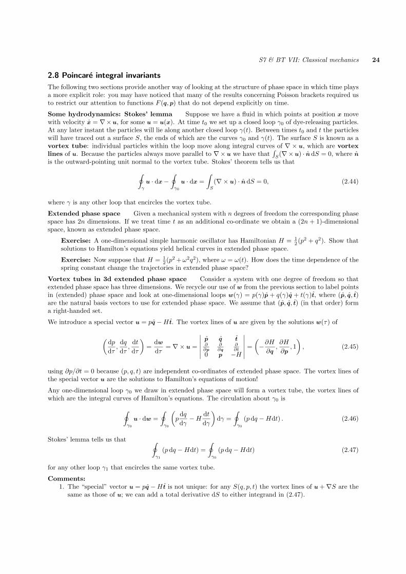
2.8 Poincare integral invariants
The following two sections provide another way of looking at the structure of phase space in which time playsa more explicit role: you may have noticed that many of the results concerning Poisson brackets required usto restrict our attention to functions F (q, p) that do not depend explicitly on time.
Some hydrodynamics: Stokes’ lemma Suppose we have a fluid in which points at position x movewith velocity x = ∇×u, for some u = u(x). At time t0 we set up a closed loop γ0 of dye-releasing particles.At any later instant the particles will lie along another closed loop γ(t). Between times t0 and t the particleswill have traced out a surface S, the ends of which are the curves γ0 and γ(t). The surface S is known as avortex tube: individual particles within the loop move along integral curves of ∇ × u, which are vortexlines of u. Because the particles always move parallel to ∇× u we have that
∫S
(∇× u) · ndS = 0, where nis the outward-pointing unit normal to the vortex tube. Stokes’ theorem tells us that
∮
γ
u · dx−∮
γ0
u · dx =
∫
S
(∇× u) · ndS = 0, (2.44)
where γ is any other loop that encircles the vortex tube.
Extended phase space Given a mechanical system with n degrees of freedom the corresponding phasespace has 2n dimensions. If we treat time t as an additional co-ordinate we obtain a (2n + 1)-dimensionalspace, known as extended phase space.
Exercise: A one-dimensional simple harmonic oscillator has Hamiltonian H = 12 (p2 + q2). Show that
solutions to Hamilton’s equations yield helical curves in extended phase space.
Exercise: Now suppose that H = 12 (p2 +ω2q2), where ω = ω(t). How does the time dependence of the
spring constant change the trajectories in extended phase space?
Vortex tubes in 3d extended phase space Consider a system with one degree of freedom so thatextended phase space has three dimensions. We recycle our use of w from the previous section to label pointsin (extended) phase space and look at one-dimensional loops w(γ) = p(γ)p + q(γ)q + t(γ)t, where (p, q, t)are the natural basis vectors to use for extended phase space. We assume that (p, q, t) (in that order) forma right-handed set.
We introduce a special vector u = pq −H t. The vortex lines of u are given by the solutions w(τ) of
(dp
dτ,
dq
dτ,
dt
dτ
)=
dw
dτ= ∇× u =
∣∣∣∣∣∣
p q t∂∂p
∂∂q
∂∂t
0 p −H
∣∣∣∣∣∣=
(−∂H∂q
,∂H
∂p, 1
), (2.45)
using ∂p/∂t = 0 because (p, q, t) are independent co-ordinates of extended phase space. The vortex lines ofthe special vector u are the solutions to Hamilton’s equations of motion!
Any one-dimensional loop γ0 we draw in extended phase space will form a vortex tube, the vortex lines ofwhich are the integral curves of Hamilton’s equations. The circulation about γ0 is
∮
γ0
u · dw =
∮
γ0
(p
dq
dγ−H dt
dγ
)dγ =
∮
γ0
(p dq −Hdt) . (2.46)
Stokes’ lemma tells us that ∮
γ1
(pdq −Hdt) =
∮
γ0
(p dq −Hdt) (2.47)
for any other loop γ1 that encircles the same vortex tube.
Comments:1. The “special” vector u = pq −H t is not unique: for any S(q, p, t) the vortex lines of u+∇S are the
same as those of u; we can add a total derivative dS to either integrand in (2.47).
25 S7 & BT VII: Classical mechanics
2. If we choose γ0 and γ1 to lie on constant-t slices, t = t0 and t = t1 respectively, of extended phasespace, then dt = 0 and (2.47) becomes
∮
t0
p dq =
∮
t1
pdq ⇒∫
S(t0)
dp dq =
∫
S(t1)
dpdq. (2.48)
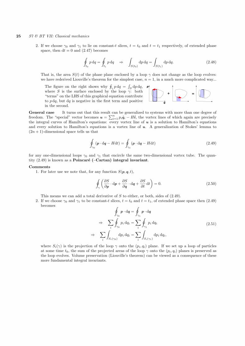
That is, the area S(t) of the phase plane enclosed by a loop γ does not change as the loop evolves:we have rederived Liouville’s theorem for the simplest case, n = 1, in a much more complicated way...
+ =
p
q
The figure on the right shows why∮γpdq =
∫S
dp dq,where S is the surface enclosed by the loop γ: both“terms” on the LHS of this graphical equation contributeto p dq, but dq is negative in the first term and positivein the second.
General case It turns out that this result can be generalized to systems with more than one degree offreedom. The “special” vector becomes u =
∑ni=1 piqi − H t, the vortex lines of which again are precisely
the integral curves of Hamilton’s equations: every vortex line of u is a solution to Hamilton’s equationsand every solution to Hamilton’s equations is a vortex line of u. A generalization of Stokes’ lemma to(2n+ 1)-dimensional space tells us that
∮
γ0
(p · dq −Hdt) =
∮
γ1
(p · dq −Hdt) (2.49)
for any one-dimensional loops γ0 and γ1 that encircle the same two-dimensional vortex tube. The quan-tity (2.49) is known as a Poincare (–Cartan) integral invariant.
Comments1. For later use we note that, for any function S(p, q, t),
∮
γ
(∂S
∂p· dp+
∂S
∂q· dq +
∂S
∂tdt
)= 0. (2.50)
This means we can add a total derivative of S to either, or both, sides of (2.49).2. If we choose γ0 and γ1 to be constant-t slices, t = t0 and t = t1, of extended phase space then (2.49)
becomes ∮
γ0
p · dq =
∮
γ1
p · dq
⇒∑
i
∮
γ0
pi dqi =∑
i
∮
γ1
pi dqi
⇒∑
i
∫
Si(γ0)
dpi dqi =∑
i
∫
Si(γ1)
dpi dqi,
(2.51)
where Si(γ) is the projection of the loop γ onto the (pi, qi) plane. If we set up a loop of particlesat some time t0, the sum of the projected areas of the loop γ onto the (pi, qi) planes is preserved asthe loop evolves. Volume preservation (Liouville’s theorem) can be viewed as a consequence of thesemore fundamental integral invariants.

S7 & BT VII: Classical mechanics 26
2.9 Canonical maps
We have seen how easy it is to change variables q → Q in the Lagrangian formulation of mechanics. Theprice we pay for the more interesting and powerful structure of phase space in Hamiltonian mechanics isthat co-ordinate transformations are not so straightforward.
In this section we investigate how to change to new phase-space co-ordinates (Q,P ),
Qi = Qi(q, p, t),
Pi = Pi(q, p, t),(i = 1, . . . , n), (2.52)
that preserve the Poincare invariants of the previous section. First, some definitions: If for any loop γ inextended phase space we have that
∮
γ
(P · dQ−Kdt) =
∮
γ
(p · dq −Hdt) (2.53)
in which the function K(Q,P , t) is independent of the choice of γ, then the transformation (2.52) is called acanonical map (or a canonical transformation) and the new co-ordinates (P ,Q) are called canonicalco-ordinates.†Evolution under time is an example of a canonical map. To see this, suppose that we define (Q,P ) tobe the values that (q, p) will have one second in the future. Then (2.53) is clearly satisfied if we takeK(Q,P , t) = H(Q,P , t+ 1 sec).
Hamilton’s equations in the new co-ords The RHS of (2.53) is∮γu·dw, where w = (p(γ), q(γ), t(γ))
and u =∑i piqi −H t. We have already seen that the vortex lines for this u are given by
qi =∂H
∂pi, pi = −∂H
∂qi. (2.54)
Similarly, the LHS of (2.53) is∮γU ·dW , where W = (P (γ),Q(γ), t(γ)) and U =
∑i PiQi−K t. The vortex
lines of U are clearly given by
Q =∂K
∂P, P = −∂K
∂Q. (2.55)
Both (2.54) and (2.55) describe the same vortex lines in the same extended phase space, but expressedin different co-ordinates. Therefore Hamilton’s equations in the new co-ordinates are given by (2.55) withHamiltonian K(Q,P , t).
Generating functions Equation (2.53) can hold for all loops γ only if the integrands differ by a totalderivative dS of any well-behaved function S(P ,Q, t):
P · dQ−Kdt+ dS = p · dq −Hdt. (2.56)
A powerful way of constructing canonical maps is by playing with the function S. Let us assume that we canexpress P = P (q,Q, t) so that we can eliminate P from S to obtain S = F1(q,Q, t), a function of both theold and new co-ordinates and time, but not the momenta. Substituting this S = F1 into (2.56) and usingthe chain rule gives
P · dQ−Kdt+∂F1
∂q· dq +
∂F1
∂Q· dQ+
∂F1
∂tdt = p · dq −Hdt. (2.57)
As (dq,dQ,dt) can be varied independently (the equality above has to hold for any loop γ) we must have
p =∂F1
∂q, P = −∂F1
∂Q, K = H +
∂F1
∂t. (2.58)
† NB: Some books define a canonical map as one that preserves the form of Hamilton’s equations. Ourcondition (2.53) is more stringent.

27 S7 & BT VII: Classical mechanics
where H in the last equation is to be interpreted as the original H(q, p, t) substituting for q = q(Q,P , t), p =p(Q,P , t) to make it a function of (Q,P , t). Thus the function F1(q,Q, t) generates an implicit transformationfrom (q, p)→ (Q,P ). By construction, it satisfies the condition (2.53) and therefore is canonical.
Exercise: What mapping is generated by F1 = q·Q? Show that the Hamiltonian H(q, p) = 12 (p2+ω2q2)
is transformed to K(Q,P ) = 12 (Q2 + ω2P 2).
Unfortunately, generating functions of the form F1(q,Q, t) are not suitable for constructing mappings closeto the identity. So, instead of writing S = F1(q,Q, t), let us take
S = −P ·Q+ F2(q,P , t), (2.59)
in which we treat Q as a function Q(q,P , t). Substituting this into (2.56) and using the chain rule to expanddS gives:
P · dQ−Kdt− P · dQ−Q · dP +∂F2
∂q· dq +
∂F2
∂P· dP +
∂F2
∂tdt = p · dq −Hdt. (2.60)
One way of explaining the −P · Q term that appears in (2.59) that it comes from taking the Legendretransform of F1. An alternative, simpler approach is to note that (a) we are free to choose (almost) whateverwe like for S and (b) including −P ·Q in S nicely cancels out the P ·dQ on the LHS of (2.56). As (dP ,dq,dt)vary independently, we must have that
p =∂F2
∂q, Q =
∂F2
∂P, K = H +
∂F2
∂t. (2.61)
This is another implicit canonical mapping between (q, p, t) and (Q,P , t).
Exercise: Show that F2(q,P ) = q · P generates the identity map. What mapping does F2(q,P ) =q · P + εn · q produce? What about F2 = q · P + εn · P ?
Exercise: Show that for small λ the generating function F2(q,P ) = q · P + λG(q,P ) produces theinfinitesmal map (2.41). (Use the fact that P → p as λ→ 0.)
Is a given mapping canonical? A simple way of testing whether a mapping is canonical is by examiningP · dQ− p · dq. If that can be expressed as a total derivative dS(p, q, t) or dS(P ,Q, t) then the mapping iscanonical.
Exercise: Show that the mapping Q = − log p, P = pq is canonical. Find a function F1(q,Q) thatgenerates this mapping. Find another generating function of the form F2(q, P ).
Another test is to return to the definition (2.53) of a canonical map and to check whether
∑
i
∫
Si(γ)
dPidQi =∑
i
∫
si(γ)
dpidqi (2.62)
for all loops γ, where si(γ) and Si(γ) are the projections of γ onto the (pi, qi) and (Pi, Qi) planes. Let uslook at the projections of the (pk, qk) planes onto all of the (Qi, Qj), (Pi, Pj) and (Pi, Qj) planes. We havethat
dQidQj =∑
k
(∂Qi∂qk
∂Qj∂pk
− ∂Qj∂qk
∂Qi∂pk
)dpkdqk,
dPidQj =∑
k
(∂Pi∂qk
∂Qj∂pk
− ∂Qj∂qk
∂Pi∂pk
)dpkdqk,
dPidPj =∑
k
(∂Pi∂qk
∂Pj∂pk− ∂Pj∂qk
∂Pi∂pk
)dpkdqk,
(2.63)

S7 & BT VII: Classical mechanics 28
where the quantities in parentheses are the Jacobians of the transformation from (qk, pk) to the new (Qi, Qj)etc coordinates. The only way of making (2.62) hold for all choices of the loop γ is by requiring that
∑
k
(∂Qi∂qk
∂Qj∂pk
− ∂Qj∂qk
∂Qi∂pk
)= 0,
∑
k
(∂Pi∂qk
∂Qj∂pk
− ∂Qj∂qk
∂Pi∂pk
)= δij ,
∑
k
(∂Qi∂qk
∂Qj∂pk
− ∂Qj∂qk
∂Qi∂pk
)= 0.
(2.64)
That is, for a map to be canonical, the new coords (Q,P ) must themselves satisfy the canonical commutationrelations (a.k.a. fundamental Poisson bracket relations)
[Qi, Qj ] = [Pi, Pj ] = 0, [Qi, Pj ] = δij , (2.65)
in which the Poisson brackets are understood to be evaluated with respect to the old (q, p) coordinates, asin (2.64). Equation (2.65) is a necessary and sufficient condition for (2.62) to be true: a map (q, p)→ (Q,P )is canonical if and only if the new coordinates (Q,P ) satisfy the canonical commutation relations (2.65).
Invariance of Poisson brackets under canonical maps We can use the condition (2.65) to show thatall Poisson brackets are invariant under canonical maps. To simplify notation, we introduce
w =
(q
p
)and W =
(Q
P
), (2.66)
in terms of which the relations (2.65) become simply [Wi,Wj ] = Jij , where Jij are the elements of thesymplectic matrix (2.32). Then, using expression (2.33) for the Poisson bracket of the functions A(w, t),B(w, t), we have that
[A,B]w =2n∑
α,β=1
∂A
∂wαJαβ
∂B
∂wβ=
2n∑
α,β=1
(2n∑
i=1
∂A
∂Wi
∂Wi
∂wα
)Jαβ
2n∑
j=1
∂B
∂Wj
∂Wj
∂wβ
=2n∑
i,j=1
∂A
∂Wi
2n∑
α,β=1
∂Wi
∂wαJαβ
∂Wj
∂wβ
∂B
∂Wj=
2n∑
i,j=1
∂A
∂Wi[Wi,Wj ]
∂B
∂Wj
=2n∑
i,j=1
∂A
∂WiJij
∂B
∂Wj= [A,B]W .
(2.67)
So, canonical maps preserve all Poisson brackets.
Exercise: We have been cavalier about the choice of signs in the Jacobians in equation (2.63) above.Here is how to show that the signs in that expression are correct. Any pair of n-dimensional vectors (a, b)defines a parallelogram in n-dimensional space. We define the oriented area of the projection of thisparallelogram onto the (xi, xj) plane to be (dxi∧dxj)(a, b) = aibj−ajbi. Show that (dxi∧dxj)(b,a) =−(dxi ∧ dxj)(a, b) = (dxj ∧ dxi)(a, b).Given new coordinates X = X(x), the projection of the (a, b) parallelogram onto the (Xi, Xj) plane is
(dXi ∧ dXj)(a, b) =
(∑
k
∂Xi
∂xkdxk ∧
∑
l
∂Xj
∂xldxl
)(a, b) =
∑
kl
∂Xi
∂xk
∂Xj
∂xl(dxk ∧ dxl)(a, b). (2.68)
Hence show that the condition∑i(dPi ∧ dQi)(a, b) =
∑i(dpi ∧ dqi)(a, b) for all (a, b) implies (2.64).
Now read §§12–16, 18–20, 32–48 of Arnol’d.
29 S7 & BT VII: Classical mechanics
3 Linearisation and small oscillations (WIP)
A mechanical system is in equilibrium if all time derivatives vanish. In particular, if q = q0 is an equilibriumconfiguration, then we must have q = 0 and, from the EL equation, ∂L/∂q = 0 too. To study the behaviourof a system close to equilibrium, the usual first step is to linearize the equations of motion. This reducesthe problem to modelling a coupled set of simple harmonic oscillators, making it easy to test whether theequilibrium is stable or unstable, to calculate the frequencies with which the system “rings” when knocked,and much more.
Expanding L(q, q) to second order as a Taylor series about (q, q) = (q0, 0),
L(q + h, q + h) = L(q0, 0) +∑
i
hi
(∂L
∂qi
)
(q0,0)
+∑
i
hi
(∂L
∂qi
)
(q0,0)
+ 12
∑
ij
[hiFijhj + hiCij hj + hiC
Tijhj + hiMij hj
]+O(h3),
(3.1)
where the constants Fij = Fji ≡ ∂2L/∂qi∂qj , Mij = Mji ≡ ∂2L/∂qi∂qj and Cij = CTji ≡ ∂2L/∂qi∂qj , allevaulated at (q, q) = (q0, 0). Remembering that ∂L/∂qi = 0 at equilibrium, it is easy to see that none of thefirst three terms affect the equations of motion. The linearized EL equation for hk is then
d
dt
1
2
∑
i
hiCik + 12
∑
j
CTkjhj +∑
j
Mkj hj
−
∑
j
Fkjhj + 12
∑
j
Ckj hj + 12
∑
i
hiCTik
= 0
⇒∑
i
[Mkihi + (Cik − Cki)hi − Fkihi
]= 0.
(3.2)
The solutions to this homogeneous linear equation are of the form h(t) = Q exp(iωt), with the vector Q andω related through the eigenvalue equation
[ω2M − iωC + F ]Q = 0, (3.3)
where Cij = (Cij−Cij) is the antisymmetric part of C. Taking the determinant of this, the eigenfrequenciesω are given by the roots of
det(F − iωC + ω2M) = 0, (3.4)
The system is (linearly) stable if all the eigenfrequencies are real.
For most problems
L = T − V = 12
∑
ij
aij(q)qiqj − V (q), (3.5)
with some symmetric functions aij(q) = aji(q) such that the kinetic energy is a positive definite quadraticform in the velocities. For typical cases it turns out that Mij = aij(q0), Fij = −∂2V/∂qi∂qj and Cij =0. An exception is when there are velocity-dependent forces (e.g., motion in a rotating frame or in anelectromagnetic field). We simply ignore such problems in the following and assume from now on thatCij = 0.
It is easy to see that each of the eigenfrequencies ω is either purely real or purely imaginary. Substitutinghi = Qi exp(iωt) into (3.2), multiplying by Q?k, summing over k and rearranging gives
ω2 = −∑
ki
FkiQ?kQi/
∑
ki
MkiQ?kQi. (3.6)
Each of the sums is real, because
(∑
ki
MkiQ?kQi
)?=∑
ki
MkiQkQ?i =
∑
ki
MikQkQ?i =
∑
ki
MkiQ?kQi, (3.7)
S7 & BT VII: Classical mechanics 30
by the symmetry of Mki (and Fki), and swapping labels (i, k) in the last step. Since the kinetic energyT = 1
2Mij hihj is a positive definite quadratic form, it follows that all ω2 > 0 (and therefore the system isstable) if q0 is a local minimum of V .
Normal co-ordinates If the eigenfrequencies ωα obtained by solving (3.4) are distinct, then the corre-sponding eigenvectors Qα are orthogonal in the sense that
QTβMQα = 0, if ωα 6= ωβ . (3.8)
This follows on multiplying the (C = 0) eigenvalue equation (3.4)
(F + ω2αM)Qα = 0 (3.9)
by another eigenvector Qβ and then using the symmetry of F and M to show that (ωβ − ωα)QTαMQβ = 0.The importance of this is that any small oscillation h(t) that satisfies the linearized equation of motion (3.2)can be decomposed into a sum of normal modes,
h(t) =∑
α
aαQα cos(ωαt+ φα), (3.10)
where the amplitudes aβ and phases φβ can be found by premultiplying (3.10) by QTβM to obtain
QTβMh(t) = aβ cos(ωβ + φβ) (3.11)
(assuming the Qi are normalized such that QTβMQα = δαβ). Thus for each β, QTβMh(t) is a combination ofthe original co-ordinates that oscillates sinusoidally at angular frequency ωβ , regardless of how the systemwas set into motion. A combination of the co-ordinates that inevitably oscillates sinusoidally is called anormal co-ordinate.
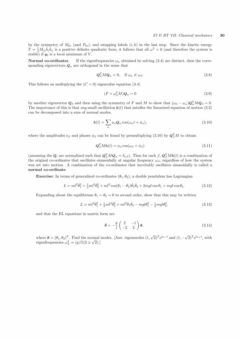
Exercise: In terms of generalized co-ordinates (θ1, θ2), a double pendulum has Lagrangian
L = ml2θ21 + 1
2ml2θ2
2 +ml2 cos(θ1 − θ2)θ1θ2 + 2mgl cos θ1 +mgl cos θ2. (3.12)
Expanding about the equilibrium θ1 = θ2 = 0 to second order, show that this may be written
L ' ml2θ21 + 1
2ml2θ2
2 +ml2θ1θ2 −mglθ21 − 1
2mglθ22, (3.13)
and that the EL equations in matrix form are
θ = −gl
(2 −1−2 2
)θ, (3.14)
where θ = (θ1, θ2)T . Find the normal modes. [Ans: eigenmodes (1,√
2)T eiω−t and (1,−√
2)T eiω+t, witheigenfrequencies ω2
± = (g/l)(2±√
2).]
31 S7 & BT VII: Classical mechanics
Attic?
A Rigid bodies?
A.1 Constraints?
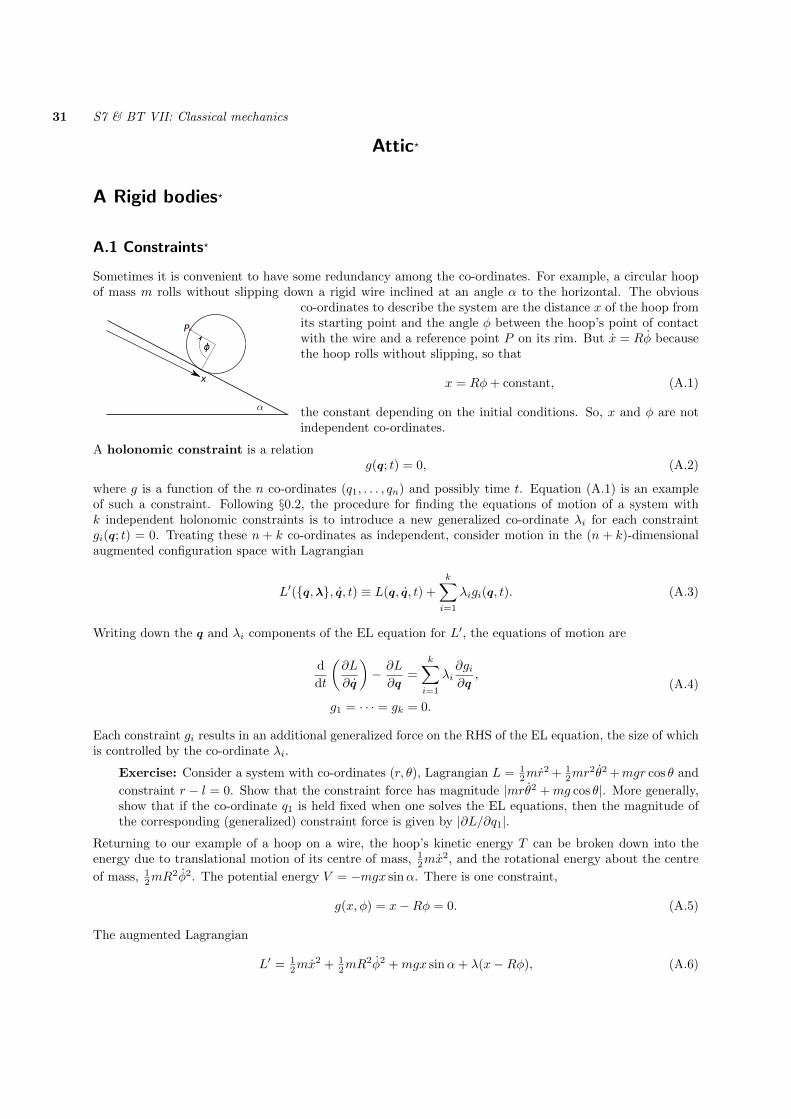
Sometimes it is convenient to have some redundancy among the co-ordinates. For example, a circular hoopof mass m rolls without slipping down a rigid wire inclined at an angle α to the horizontal. The obvious
co-ordinates to describe the system are the distance x of the hoop fromits starting point and the angle φ between the hoop’s point of contactwith the wire and a reference point P on its rim. But x = Rφ becausethe hoop rolls without slipping, so that
x = Rφ+ constant, (A.1)
the constant depending on the initial conditions. So, x and φ are notindependent co-ordinates.
A holonomic constraint is a relationg(q; t) = 0, (A.2)
where g is a function of the n co-ordinates (q1, . . . , qn) and possibly time t. Equation (A.1) is an exampleof such a constraint. Following §0.2, the procedure for finding the equations of motion of a system withk independent holonomic constraints is to introduce a new generalized co-ordinate λi for each constraintgi(q; t) = 0. Treating these n + k co-ordinates as independent, consider motion in the (n + k)-dimensionalaugmented configuration space with Lagrangian
L′(q,λ, q, t) ≡ L(q, q, t) +
k∑
i=1
λigi(q, t). (A.3)
Writing down the q and λi components of the EL equation for L′, the equations of motion are
d
dt
(∂L
∂q
)− ∂L
∂q=
k∑
i=1
λi∂gi∂q
,
g1 = · · · = gk = 0.
(A.4)
Each constraint gi results in an additional generalized force on the RHS of the EL equation, the size of whichis controlled by the co-ordinate λi.
Exercise: Consider a system with co-ordinates (r, θ), Lagrangian L = 12mr
2 + 12mr
2θ2 +mgr cos θ and
constraint r − l = 0. Show that the constraint force has magnitude |mrθ2 +mg cos θ|. More generally,show that if the co-ordinate q1 is held fixed when one solves the EL equations, then the magnitude ofthe corresponding (generalized) constraint force is given by |∂L/∂q1|.
Returning to our example of a hoop on a wire, the hoop’s kinetic energy T can be broken down into theenergy due to translational motion of its centre of mass, 1
2mx2, and the rotational energy about the centre
of mass, 12mR
2φ2. The potential energy V = −mgx sinα. There is one constraint,
g(x, φ) = x−Rφ = 0. (A.5)
The augmented Lagrangian
L′ = 12mx
2 + 12mR
2φ2 +mgx sinα+ λ(x−Rφ), (A.6)

S7 & BT VII: Classical mechanics 32
for which the EL equations ared
dtmx−mg sinα = λ,
d
dtmR2φ = −λR,
x−Rφ = 0.
(A.7)
Using the third equation to eliminate φ from the second, we have that ddtmx = −λ. Substituting this into
the first equation and eliminating λ, gives
x = 12g sinα. (A.8)
So the hoop rolls down the plane with only half the acceleration it would have in the frictionless case.
Not all constraints can be written as g(x, t) = 0. An example of a system with such a non-holonomicconstraint is a hoop rolling without slipping down a plane instead of along a wire. Natural co-ordinatesto use are the location (x, y) of the hoop’s centre, the orientation φ of a reference a point on the rim of thehoop and another angle θ giving the orientation of the hoop in the plane. The no-slip conditions mean thatthe hoop’s velocity satisfies
x = Rφ sin θ, y = Rφ cos θ, (A.9)
but these cannot be integrated to give an expression of the form g(x, y, θ, φ, t) = 0. To see this, think ofrolling the hoop on closed circuits of different lengths around the plane, returning to the starting position(x, y) with the same θ. The angle φ at the end depends on the length of the circuit.
A.2 Lagrangian mechanics of rigid bodies?
A rigid body is a system of particles having masses mi and positions xi satisfying constraints of the form|xi − xj | = rij for all pairs (i, j) of particles, where each rij is a constant.
Exercise: A rigid body moves in an external gravitational potential Φ(x). Show that extremizing theaction integral (1.3) with Lagrangian L = T − V , where T = 1
2
∑imixi
2 and V =∑imiΦ(xi), subject
to the constraints that (xi − xj)2 = r2ij , leads to the usual Newtonian equations of motion for a rigid
body:d
dtmkxk = −mi
∂Φ
∂xk+∑
j 6=k〈constraint forces〉, (A.10)
where the constraint forces are of the form λkj(xk − xj) with λkj = λjk.
Exercise: Use (A.10) to show that if there are no external forces acting on the body, then its linearmomentum
∑imixi and angular momentum
∑i xi × mixi are conserved. See §1.6 later for a more
elegant way of obtaining this result.
The configuration space of a rigid body is six dimensional. In case this is not obvious, pick any three non-collinear points x1, x2 and x3 in the body. We need three numbers to specify x1, another two for x2 (wealready know r21) and a final one to fix x3. The positions xi of all the other points in the body are thencompletely determined by the constraints |xi − x1| = ri1, |xi − x2| = ri2 and |xi − x3| = ri3, once we’vechosen whether x4 lies “above” or “below” the plane defined by (x1,x2,x3).
Let us set up a co-ordinate system that moves with the body, its origin at x1, its first basis vector r1 =(x2 − x1)/|x2 − x1|, the second, r2, orthogonal to r1 but lying in the (x1,x2,x3) plane and the third givenby r3 = r1 × r2. In this frame, the co-ordinates ri of particles in the body do not change with time, ri = 0.In the inertial x frame, the particles’ co-ordinates
xi = R+Bri, (A.11)
where R = x1 and the rotation matrix B is set by the orientation of (r1, r2, r3). We use this R and a set ofthree angles, known as Euler angles, that describe B as our six generalized co-ordinates for the body. The
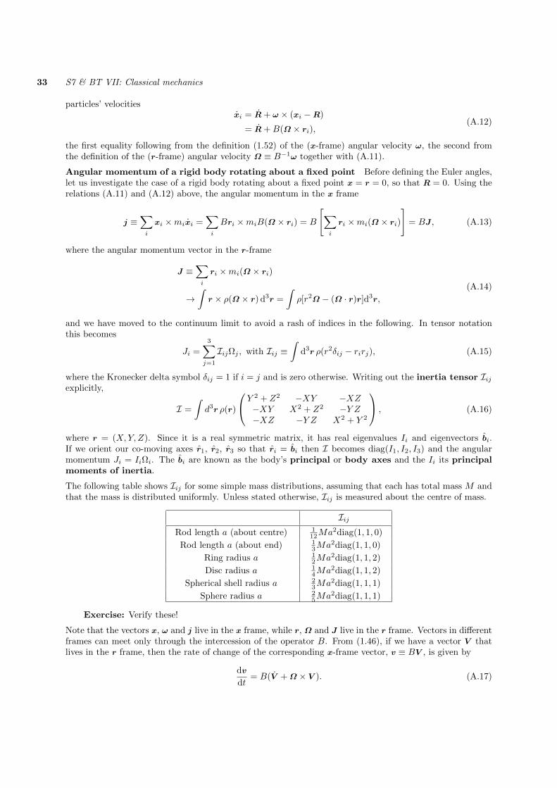
33 S7 & BT VII: Classical mechanics
particles’ velocitiesxi = R+ ω × (xi −R)
= R+B(Ω × ri),(A.12)
the first equality following from the definition (1.52) of the (x-frame) angular velocity ω, the second fromthe definition of the (r-frame) angular velocity Ω ≡ B−1ω together with (A.11).
Angular momentum of a rigid body rotating about a fixed point Before defining the Euler angles,let us investigate the case of a rigid body rotating about a fixed point x = r = 0, so that R = 0. Using therelations (A.11) and (A.12) above, the angular momentum in the x frame
j ≡∑
i
xi ×mixi =∑
i
Bri ×miB(Ω × ri) = B
[∑
i
ri ×mi(Ω × ri)]
= BJ , (A.13)
where the angular momentum vector in the r-frame
J ≡∑
i
ri ×mi(Ω × ri)
→∫r × ρ(Ω × r) d3r =
∫ρ[r2Ω − (Ω · r)r]d3r,
(A.14)
and we have moved to the continuum limit to avoid a rash of indices in the following. In tensor notationthis becomes
Ji =3∑
j=1
IijΩj , with Iij ≡∫
d3r ρ(r2δij − rirj), (A.15)
where the Kronecker delta symbol δij = 1 if i = j and is zero otherwise. Writing out the inertia tensor Iijexplicitly,
I =
∫d3r ρ(r)
Y 2 + Z2 −XY −XZ−XY X2 + Z2 −Y Z−XZ −Y Z X2 + Y 2
, (A.16)
where r = (X,Y, Z). Since it is a real symmetric matrix, it has real eigenvalues Ii and eigenvectors bi.If we orient our co-moving axes r1, r2, r3 so that ri = bi then I becomes diag(I1, I2, I3) and the angularmomentum Ji = IiΩi. The bi are known as the body’s principal or body axes and the Ii its principalmoments of inertia.
The following table shows Iij for some simple mass distributions, assuming that each has total mass M andthat the mass is distributed uniformly. Unless stated otherwise, Iij is measured about the centre of mass.
IijRod length a (about centre) 1
12Ma2diag(1, 1, 0)
Rod length a (about end) 13Ma2diag(1, 1, 0)
Ring radius a 12Ma2diag(1, 1, 2)
Disc radius a 14Ma2diag(1, 1, 2)
Spherical shell radius a 23Ma2diag(1, 1, 1)
Sphere radius a 25Ma2diag(1, 1, 1)
Exercise: Verify these!
Note that the vectors x, ω and j live in the x frame, while r, Ω and J live in the r frame. Vectors in differentframes can meet only through the intercession of the operator B. From (1.46), if we have a vector V thatlives in the r frame, then the rate of change of the corresponding x-frame vector, v ≡ BV , is given by
dv
dt= B(V +Ω × V ). (A.17)
S7 & BT VII: Classical mechanics 34
We can immediately apply this to j = BJ in the case of a free rigid body rotating about a fixed point (e.g.,centre of mass of a freely falling body). Since there are no external torques j is conserved. So,
dj
dt= B(J +Ω × J) = 0 ⇒ J +Ω × J = 0, (A.18)
which is known as Euler’s equation. In the principal-axis frame Ji = IiΩi and Euler’s equation becomes
I1dΩ1
dt= (I2 − I3)Ω2Ω3,
I2dΩ2
dt= (I3 − I1)Ω3Ω1,
I3dΩ3
dt= (I1 − I2)Ω1Ω2.
(A.19)
The motion of rigid bodies is interesting because the angular momentum J is not proportional to the angularvelocity Ω (unless I1 = I2 = I3).
Exercise: (The “tennis racquet theorem”) A rigid body rotates freely about its third principal axis,with J = (0, 0, I3Ω3). It is given a small perturbation, so that Ω1 and Ω2 are non-zero, but small.By substituting trial solutions of the form Ω1 = a1e
kt and Ω2 = a2ekt into (A.19) and neglecting
second-order terms such as Ω1Ω2, show that the motion is stable (k2 < 0) if either I3 > max(I1, I2) orI3 < min(I1, I2). Thus rotation about either the short or the long axis of a free rigid body is stable, butrotation about the intermediate axis is unstable.
Exercise: Consider a free symmetric top with I1 = I2 6= I3. Show that Ω3 is a constant of motionand that the angular velocity Ω precesses around the r3 axis with frequency
Ωp =I1 − I3I1
Ω3. (A.20)
Notice that the precession is retrograde (Ωp < 0) if I3 > I1 (i.e., if the body is oblate).
Kinetic energy of a rigid body rotating about a fixed point Using x = B(Ω×r), the kinetic energyT = 1
2
∑imix
2i becomes
T = 12
∫ρ [B(Ω × r)]T · [B(Ω × r)] d3r = 1
2
∫ρ (Ω × r)2
d3r
= 12
∫ρ[Ω2r2 − (Ω · r)2
]d3r.
(A.21)
We can rewrite the contents of the square brackets as
Ω2r2 − (Ω · r)2 =∑
ij
ΩiΩjr2δij −
∑
i
Ωiri∑
j
Ωjrj =∑
ij
ΩiΩj(r2δij − rirj), (A.22)
so thatT = 1
2
∑
ij
ΩiIijΩj = 12Ω
T · I ·Ω, (A.23)
where Iij are the components of the inertia tensor (A.15).
Exercise: Starting from (A.12), show that if we allow translational motion (R 6= 0) and we take R tobe the position of the body’s centre of mass, then the kinetic energy of the body can be split into twoparts,
T = 12MR2 + 1
2
∑
ij
ΩiIijΩj , (A.24)

35 S7 & BT VII: Classical mechanics
where M is the total mass of the body. The first term is the kinetic energy of translational motion of thebody’s centre of mass, the second the rotational kinetic energy of the body about its centre of mass.
The rest of this section explains how to obtain a Lagrangian for a body moving in a uniform gravitationalfield about a fixed point (e.g., a top spinning about a point on a table). We first introduce Euler angles.These describe the rotation matrix B and serve as our generalized co-ordinates. Then we obtain the potentialenergy and kinetic energy in terms of these angles and the principal moments of inertia of the system.
Euler angles The standard method for parametrizing B is as follows. Start with the r1, r2, r3 axescoincident with the inertial x1, x2, x3 axes. Then apply the following sequence of rotations to the former:
1. Rotate through an angle φ about the r3 = x3 axis. Under this rotation r3 = x3 is unchanged and r1
(temporarily) picks out a new direction known as the “line of nodes”. Label this direction rN .2. Rotate through an angle θ about the line of nodes (the temporary r1 axis). The line of nodes remains
fixed, and r3 comes to its final position.3. rotate through an angle ψ about the r3 axis.
Writing out this sequence of operations explicitly, we have that
r1
r2
r3
=
cosψ sinψ 0− sinψ cosψ 0
0 0 1
1 0 00 cos θ sin θ0 − sin θ cos θ
cosφ sinφ 0− sinφ cosφ 0
0 0 1
x1
x2
x3
, (A.25)
or r = Cx, where C is the product of the three rotation matrices above. Since C is orthogonal, we have thatx = CT r, or xi = Cjirj . So, a point P with co-ordinates r = riri in the r basis can be written as
a = riri = riCij xj . (A.26)
In other words, the point P has x co-ordinates x = Br, where the (co-ordinate) rotation matrix B = CT .
Exercise: It is perhaps not immediately obvious, so show that any rotation can be represented by somechoice (sometimes not unique) of Euler angles (φ, θ, ψ).
Potential energy of an axisymmetric top Assume that the top is rotationally sym-metric about the r3 axis. Then V does not change as ψ and φ are varied, because inthe definition of Euler angles the ψ and φ rotations take place about this axis. ThereforeV = mgl cos θ, where (r1, r2, r3) = (0, 0, l) is the position of the top’s centre of mass in thebody frame.
Kinetic energy in terms of Euler angles Finally, we need to express the Ω appearing in (A.23) interms of (φ, θ, ψ) and their derivatives. Between times t and t+ dt the orientation of the rigid body changesfrom (φ, θ, ψ) to (φ + dφ, θ + dθ, ψ + dψ) and the x co-ordinates of a point r = constant on the body varyfrom x to x+ dx. Since x(t) = B(t)r, we have that (to first order in dt,dφ etc)
dx = B(φ+ dφ, θ + dθ, ψ + dψ)B−1(φ, θ, ψ)x− x = ωdt× x, (A.27)
the last equality following from the definition (1.52) of angular velocity. Taking the changes in each angleseparately,
B(φ+ dφ, θ, ψ)B−1(φ, θ, ψ)x− x = ωφdt× xB(φ, θ + dθ, ψ)B−1(φ, θ, ψ)x− x = ωθdt× xB(φ, θ, ψ + dψ)B−1(φ, θ, ψ)x− x = ωψdt× x,
(A.28)
and the total angular velocity ω = ωφ + ωθ + ωψ (again, to first order). Our job is to express ωφ, ωθ andωψ in terms of either the x or the r basis. Let us do this first for the special case φ = ψ = 0. The first ofequations (A.28) is a rotation of dφ about the x3 axis, giving
ωφ = φx3 = φ sin θr2 + φ cos θr3, (A.29)
S7 & BT VII: Classical mechanics 36
because, solving (A.25) for x = (0, 0, 1)T , x3 = r2 sin θ + r3 cos θ when φ = ψ = 0. The second is a rotationof dθ about the line of nodes rN (= r1 when ψ = φ = 0). Therefore
ωθ = θr1. (A.30)
The third is a rotation of dψ about r3, soωψ = ψr3. (A.31)
Gathering these last three equations together, ω = ωφ + ωθ + ωψ = B(Ω1,Ω2,Ω3)T with
Ω1 = θ, Ω2 = φ sin θ, Ω3 = ψ + φ cos θ. (A.32)
The expression (A.23) for the kinetic energy of our axisymmetric (I1 = I2) top becomes
T = 12I1
(θ2 + φ2 sin2 θ
)+ 1
2I3
(ψ + φ cos θ
)2
. (A.33)
This is assuming that φ = ψ = 0. But for an axisymmetric top the kinetic energy cannot depend on thesecyclic co-ordinates and we can always choose the origin of reference for φ and ψ to have ψ = φ = 0. Thusthe expression holds for all ψ, φ and so the Lagrangian for an axisymmetric top moving about a fixed pointin a uniform field is
L = T − V = 12I1
(θ2 + φ2 sin2 θ
)+ 1
2I3
(ψ + φ cos θ
)2
−mgl cos θ. (A.34)
Exercise: (optional detour) It is also possible to obtain Ω in terms of (φ, θ, ψ) without assuming thatφ = ψ = 0. Show that for general (φ, θ, ψ),
Ω = φx3 + θrN + ψr3
= [φ sin θ sinψ + θ cosψ]r1 + [φ sin θ cosψ − θ sinψ]r2 + [ψ + φ cos θ]r3
, (A.35)
using (A.25) to obtain x3 and rN in terms of the ri. Substitute this into the expression (A.23) for thekinetic energy and show that it reduces to (A.33) when I1 = I2.
Exercise: Free symmetric top revisited We have already seen how the angular velocity Ω of afree symmetric top precesses about r3 at a rate Ωp = Ω3(I1 − I3)/I1 (A.20). Now let us look at itfrom an inertial frame. By substituting ψ = Ωpt into (A.35) or otherwise explain how one can identify
ψ with the precession rate Ωp. Use this together with Ω3 = ψ + φ cos θ from (A.35) to show that
φ = I3Ω3/I1 cos θ and hence that the wobble rate φ of a uniform disc (I1 = I2 = 12I3) satisfies φ ' −2ψ
when Ω1,Ω2 Ω3.
Pinned axisymmetric top in uniform gravitational field The generalized momenta
pφ =∂L
∂φ= φI1 sin2 θ + φI3 cos2 θ + ψI3 cos θ,
pψ =∂L
∂ψ= ψI3 + φI3 cos θ
(A.36)
in (A.34) are clearly constants of motion. So too is the energy E = T + V , which can be written as
E = 12I1θ
2 +
[(pφ − pψ cos θ)2
2I1 sin2 θ+p2ψ
2I3+mgl cos θ
]. (A.37)
This comes from using (A.36) to eliminate
ψ =pψI3− φ cos θ, φ =
pφ − pψ cos θ
I1 sin2 θ, (A.38)

37 S7 & BT VII: Classical mechanics
from the expression (A.33) for T in favour of the constants pψ, pφ. Therefore the problem reduces to motionin the one-dimensional potential Veff(θ) given by the contents of the square bracket in (A.37).
Substituting u = cos θ, equation (A.37) becomes
E = 12
I1u2
1− u2+
(pφ − pψu)2
2I1(1− u2)+p2ψ
2I3+mglu, (A.39)
or, rearranging,u2 = (α− βu)(1− u2)− (a− bu)2 ≡ f(u) (A.40)
with constants
a =pφI1, b =
pψI1, α =
1
I1
(2E − pψ
I3
), β =
2mgl
I1> 0. (A.41)
f(u) is a cubic with f(u)→∞ as u→∞. Since u = cos θ, u must lie between -1 and 1. Looking at (A.41)we see that f(±1) < 0 unless a = b. Therefore f(u) has two roots u1, u2 in the interval −1 < u < 1, betweenwhich u2 = f(u) > 0. This means that the inclination θ nutates (nods) between two values θ1 = cos−1 u1
and θ2 = cos−1 u2. Meanwhile the azimuthal angle φ precesses at a rate
φ =a− bu1− u2
. (A.42)
If u = b/a lies between u1 and u2, φ changes sign meaning that the curve traced by the top on the (θ, φ)sphere has loops – see lectures!