S tatistical Analysis of Sum-of-Sinusoids Fading Channel Simulators

Marius Pop

A thesis subrnitted to the Depanment of Electrical and Cornputer Engineering in confomiity with the requirements for the degree of

Master of Science (Engineering)

Queen's University

February 1999

copyright @ Marius Pop, 1999

National Library 1+1 .,,,da Bibliothèque nationale du Canada

Acquisitions and Acquisitions et Bibliographie Services services bibliographiques

395 Wellington Street 395. rue Wellington Ottawa ON K1A ON4 OnawaON K1AON4 Cano& Canada

The author has granted a non- L'auteur a accordé m e licence non exclusive licence dowing the exclusive permettant à la National Library of Canada to Bibliothèque nationale du Canada de reproduce, l o q distribute or sell reproduire, preter, distribuer ou copies of this thesis in microform, vendre des copies de cette thèse sous paper or electronic formats. la fome de microfiche/fïlrn, de

reproduction sur papier ou sur format électronique.

The author retains ownership of the L'auteur conserve la propriété du copyright in this thesis. Neither the droit d'auteur qui protège cette thèse. thesis nor substantial extracts fiom it Ni la thèse ni des extraits substantiels may be printed or otherwise de celle-ci ne doivent être imprimés reproduced without the author's ou autrement reproduits sans son permission. autoisation.

Abstract

Multipath propagation leadinp to Rayleigh fading in wireless channels can be adequately

modelled through the use of sum-of-sinusoids simulators. We present a quick overview

of the work carried out thus far in this area, culminating with the development of Clarke's

model [3]. A popular sum-of-sinusoids fading channel simulator is derived from this model

by Jakes [23]. In general, in order to assess the performance of channel simulators one

needs to determine the statistics of the fading channel. A cornmon way of accornplishing

this is sending a sine wave across the channel and then determining the statistics of the

output signal; even this simplified problem rnay not always be tractable. In the case of sum-

of-sinusoids simulators, however, we are able to derive the envelope and phase probability

density functions of the fading signal produced by the simulator, given that a sine wave was

sent. In addition, we determine the autocorrelation function.

Once the statistics of the sum-of-sinusoids simulators are developed, we apply them

to Clarke's model and Jakes' fading channel simulator in order to determine whether the

simplifications made by Jakes are justified. We find they are not. In particular, while the

signal produced by Clarke's mode1 is wide-sense stationary, the signal produced by Jakes'

simulator is not. We attempt to improve the performance of Jakes' sirnulator and find

that introduction of random phase shifts in the low-frequency oscillators does produce a

wide-sense stationary signal. However, the phase shifts of the resulting fading signal are

only uncorrelated; they are not independent, as in the signal generated by Clarke's model.

Therefore, we do not solve the underlying problem with Jakes' simulator.

Also presented in this thesis are quality measures of the fading signal produced by

sum-of-sinusoids simulators. These rneasures are based on the results developed for the

envelope probability density functions, envelope distribution hnction, as well as the auto-

correlation function. We present examples of how such quality rneasures may be derived

and how they may aid in the proper choice of the number of low-frequency oscillators, or

equivaiently, sinusoids, which need to be incorporated in the simulators.

Acknowledgments

1 would like to express my gratitude and appreciation to my supervisor, Dr. N o m Beaulieu,

for making this work possible. As well, 1 would like to thank Dr. Jon Davis for help with

some of the matenal in Chapter 3. Ed Chow's encouragement and help with various statis-

tics topics is also much appreciated. 1 would also like to thank Dave Young for numerous

hours of conversation on the topic of fading channel simuiators, Chris Tan for expert help

with computer problems, and Dave Paranchych for supplying the template upon which this

thesis is based.

1 would like to thank al1 the other members of the wireless laboratory, Phi1 BOU, Xiao-

dai Dong, Andrew Toms, and Phi1 Vigneron, as well as rny classrnates, Kareem Baddour,

Kim Edwards. Mike Hubbard, Shafique Jamal, and Serge Mister for the countless hours of

entertainment and support.

Last but not least, I would like to thank my best fnend in the whole wide world, Leissa

Smith, for her patience and support during the completion of this thesis.

Contents

Abstract i

Acknowledgments ii

List of Figures vi

List of Abbreviations and SymboIs vii

1 Introduction 1

1 . 1 Outline of the thesis . . . . . . . . . . . . . . . . . . . . . . - . . . . . . . 3

1.2 Contributions of the thesis . . . . . . . . . . . . . . . . . . . . . . . . . . 5

1.3 Thesis notation . . . . . . . . . . . . . . . . . . . . . . . . . . . . . . . - 6

2 Jakes' Simulator and Patzold's Analysis 9

2.1 Previouswork . . . . . . . . . . . . . . . . . . . . . . . . . . - . . . . . . 9

2.2 Jakes' fading channel simulator . . . . . . . . . . . . . . . . . . . . . . . . 14

2.2.1 AnoteonthepdfofB, . . . . . . . . . . . . . . . . . . . . . . . . 19

2.3 Patzold's analysis . . . . . . . . . . . . . . . . . . . . . . . . . . . . . . - 23

2.4 Problems with the simulator . . . . . . . . . . . . . . . . . . . . . . . . . 27

3 Statistical Properties of Sumsf-Sinusoids Sirnulators 31

3.1 First-order statistics . . . . . . . . . . . . . . . . . . . . . . . . . . . . . . 3 1

3.1.1 The envelope and phase pdf's of Clarke's mode1 . . . . . . . . . . 42

. . . . . . . . . . 3.1.2 The envelope and phase pdf's of Jakes' simulator 43

. . . . . . . . . . . . . . . . . . . . . . . . . . . . 3.2 Second order statist, ics 46

. . . . . . . . . . . . . . . . . . . . . . . . . . . . 3.2.1 Clarke's mode1 48

3.2.2 Non-stationarity of Jakes' simulator . . . . . . . . . . . . . . . . . 54

3.2.3 Ergodicity of the fading signal . . . . . . . . . . . . . . . . . . . . 59

. . . . . . . . . . . . . . . . . . . . . . . . . . . . . . . . . . . 3.3 Summary 66

4 Improving Jakes' Sirnulator 68

. . . . . . . . . . . . . . . . . . . . . . 4.1 Understanding Jakes' assumptions 68

. . . . . . . . . . . . . . . . . 4.2 A first attempt at improving Jakrs' simulator 74

. . . . . . . . . . . . . . . 4.3 A second attempt at improving lakes' simulator 78

. . . . . . . . . . . . . . . . . . . . . . . 4.4 A closer look at Clarke's formula 83

5 Quantifying the Inaccuracies in Clarke's Mode1 90

. . . . . . . . . . . . . . . . . . . . . . . . . . . . . . 5.1 First order statistics 91

. . . . . . . . . . . . . . . . . . . . . . . . . . . . 5.2 Second order statistics 98

. . . . 5.3 Relating the number of low-frequency oscillators to the inaccuracies 107

6 Conclusion

References 112

Vita 116

List of Figures

A typical component wave (after [3, p. 9611). Note that the mobile receiver

is moving in the direction of the positive x-axis. . . . . . . . . . . . . . . . 12

Syrnrnetry imposed by Jakes on the angles of arrival and the number of rays

following the reduction. . . . . . . . . . . . . . . . . . . . . . . . . . . . . 17

Jakes' fading channel simulator (after [23, p. 701). . . . . . . . . . . . . . . 18

First step in surnrning two-dimensional independent random vectors of unit

length. Note that only points on the unit circle c m be reached. . . . . . . . 34

First two steps in surnming two-dimensional independent random vectors

of unit length. . . . . . . . . . . . . . . . . . . . . . . . . . . . . . . . . . 35

Envelope pdf of the signal generated by Clarke's model for various num-

bers of low-frequency oscillators. . . . . . . . . . . . . . . . . . . . . . . . 4 1

Variation with time of the envelope pdf of the signal produced by Clarke's

model, for N = 34. . . . . . . . . . . . . . . . . . . - . . . . . . . . . . . 44

Variation with time of the envelope pdf of the signal produced by M e s '

simulator. Here, the value of M = 8 corresponds to N = 34 in Figure 3.4. . 47

Lowpass equivalent form of the autocorrelation function of R( t ) , for N =

3 4 , w , = 1. . . . . . . . . . . . . . . . . . . . . . . - . . . . . . . . . . . 53

Lowpass equivaient form of the autocorrelation function of R(r ) , for M = 8

corresponding to N = 34 in Figure 3.6, and om, = 1. . . . . . . . . . . . . . 58

Improving Jakes' simulator by the introduction of sine terms. . . . . . . . . 75

4.2 Improving Jakes' simulator by the introduction of random phases in the

low-frequency oscillaton . . . . . . . . . . . . . . . . . . . . . . . . . . . . 79

. . . . . . . . . . . . . . . . . . . . . 3.3 Complete simulator of fading channel 85

4.4 Simplified simulator obtained for the case N = 4M + 2 and an = 9. n =

. . . . . . . . . 1. .... N . The gains are defined in equations (4.41) - (4.48). 88

Variation of maximum absolute error of the envelope pdf with the number

. . . . . . . . . . . . . . . . . . . . . . . of oscillators N in Clarke's mode1 92

Variation of maximum absolute error in the envelope cdf of the signal pro-

. . . . . . . . . . duced by Clarke's mode1 with the number of oscillators N 94

Probability plot for the envelope cdf of the signal produced by Clarke's

. . . . . . . . . . . . . . . . . . . . . . . . . . . . . . mode1 for various N 96

Close-up of probability plot for the envelope cdf of the signai produced by

. . . . . . . . . . . . . . . . . . . . . . . . . . Clarke's mode1 for various N 97

Approximating Jo(x) via the rnidpoint nile. x = 7 and M = 10 . Here. g(u) =

. . . . . . . . . . . . . . . . . . . . . . . . . . . . . . . . . . ~c0,(,,0,1,) 7E LOO

Variation of autocorrelation function breakpoint with the number of low-

frequency oscillaton (nurnber of distinct Doppler frequency shifts M and

. . . . . . . . . . . . . . . . . . . . . . . . . . . . . . the error level EIeWI 102

. . . . . . . . . . . . . . . . . . . . . . . . . . . . . . Detail of Figure 5.6. 103

. . . . . . . . . . . . . . . . . . . . . Simulator autocorrelation for N = 17 105

. . . . . . . . . . . . . . . . . . . . . Simulator autocorrelation for N = 18 106

List of Abbreviations and Symbols

Symbol

cdf

i.i.d.

jpdf

pdf

Defini tion

cumulative distribution func tion

independent and identically distributed

joint probability density function

probability density function

randorn variabIe

time average operator

statistical expectation operator

Fourier transform operator

real part operator

variance operator

angle of arrivai of nth amiving ray

gain of rzth low-frequency oscillator

mean hinction of stochastic process R(t)

charac tenstic h c t i o n corresponding to the joint probability

density function describing the nth randorn vector in the sum

of N two-dimensional independent random vectors

phase shift of nth arriving ray, in radians

random offset phase of the nth low-frequency oscillator

radian frequency, in radiansk

carrier frequency, in radims/s

vii

maximum Doppler frequency shift, in radiands

Doppler frequency shift of nth miving ray, in radiansk

time lag

rmdom variable representing the direction from the positive x-axis

of the nth randorn vector in the sum of N independent random

vectors

path attenuation coefficient for nth arriving ray

amplitude of transrnitted signal

frequency, in Hertz

cumulative distribution function of the random variable X

probability density function of the random variable X

joint probability density function of the sum of N independent

two-dimensional random vectors, in polar coordinates

joint probability density function of the nth randorn vector

in the surn of N independent two-dimensional random vectors,

in polar coordinates

joint probability density function of the surn of N independent

two-dimensional rmdom vectors, in Cartesian coordinates

joint probability density function of the nth random vector

in the sum of N independent two-dimensional random vectors, in

Cartesian coordinates

Bessel function of the first kind of order k

number of low-frequency oscillators in simplified fading

simulator, or equivalentty, the number of distinct Doppler

frequency shifts

number of Iow-frequency oscillators in fading simulator,

N = 4M + 2 in Jakes' case

random variable representing the length of the nth random

vector in the sum of N independent random vectors

statistical autocorrelation of stochastic process R(t )

statistical autocorrelation of stationary stochastic process R ( t )

stochastic process representing the received signal

reduced realization of the stochastic process R(t )

power spectral density of stochastic process R(t )

transmitted signal

time

stochastic process representing the in-phase received signd

reduced realization of the stochastic process X, ( t )

stochastic process representing the quadrature received signal

reduced realization of the stochastic process X,(t)

Chapter 1

Introduction

Humans communicate. The need to transmit information reliably has been around for as

long as humans have existed. Smoke signals, postal couriers, and telephones, are just a

few of the ways hurnans have tned to satisS, the need to communicate. Each step, brought

on by the human impetus to push the boundaries of knowledge further, was met with its

unique set of challenges. Today, most would agree the next step in this evolution is wireless

communication. Instant communication ro and from anywhere on Earth is an impressive

goal, and it too, presents a daunting set of challenges to be met before the goal is reached.

Unlike the examples mentioned above, where the effects of the medium through which

messages are exchanged are relatively well known, the same c m not be said about wireless

communication. The message, in our case a sine wave, is sent through the wireless chmnel

as electromagnetic radiation. The geography between the transmitter and receiver leads to

the electromagnetic signai being scattered and reflected, such that upon reception, it appears

as a superposition of waves. In addition, natural elements such as clouds, moisnire in the

air, and precipitation, further impair the reception by unequally attenuating waves arriving

from different directions at the receiver. Furthemore, these cornponent waves expenence

varying degrees of Doppler shift arisin; from the motion of the mobile receiver. TO make

matters worse, the characteristics of the channel Vary from hour to hour, from day to day.

Thus, the problem the wireless engineer must solve is that of reliably transmitting voice or

data over a geographically diverse and time-varying channel.

In order to design reliable systems and to assess the performance of existing systems,

the wireless engineer tests them. An obvious approach would be to test the system once it

is built. However, there are some drawbacks to this method. First, it is not cost-effective.

Building prototypes is usually expensive and tkeg are not guaranteed to work upon first

trial. Second, the time-varying nature of the channel would make it hard to distinguish the

shortcomings of a certain design from the impediments of the channel.

Fortunately, one may derive a model for the wireless channel, then implement it in

software, say. The engineer could then test the communication system under study without

ieaving the Iaboratory, or even having to manufacture a prototype. Ln addition, the effects

of the channel on the system are easier to control because the time-varying nature of the

chmnel may be removed. One inherent drawback to models, in general, is that they are only

approximations to naturally occumng phenornena. As such, the results obtained by using

these models are close to those measured directly, but not exactly the same. Of course, the

results obtained with a particular mode1 are valid only insofar as the model represents the

natural phenomenon, in our case fading.

Modeis of fading wireless channels are readily derived from physical considerations of

the fading phenomenon. It should be noted that many types of models exist. They Vary in

complexity, tirne domain implementation, Le., discrete time vs. continuous time, and un-

derlying design, Le., detenninistic vs. stochastic. The application at hand will dictate the

complexity of the model, what time domain the model will be implemented in, and whether

it will be deterministic or stochastic. For example, one may generate an approximation to

the Rayleigh fading signal by using uniform phase modulation or quadrature amplitude

modulation, Le., amplitude modulate the in-phase and quadrature components of a carrier

with a lowpass filtered Gaussian noise source [23], [24]. The main problem with the first

model is that the power spectrurn is hard to cornpute. The second model's main drawback is

that only rational forms of the fading spectrum may be obtained, whereas the fading spec-

tra encountered in practice are often non-rational. Other approaches include generation of

Rayleigh random variates via the Fourier transform [13], [22], [25]. The main difficulty

with this lies in the fact that the entire fading waveform needs to be generated before the

simulation is run. In this thesis, we look at sum-of-sinusoids models of the RayIeigh flat

fading narrowband wireless channel. The sum-of-sinusoids model is simple and may be

implemented in either discrete or continuous time. Another advantage is that the Rayleigh

fading signal is generated in real-tirne, i.e., as it is needed, in conuast with Fourier trans-

form methods. Most often, these models are described as deterministic, to emphasize that

once the parameters of the mode1 are chosen they do not change over the duration of the

simulation.

A simulator based on one such model, which has received attention lately, is Jakes'

fading channel sirnulator. The sirnulator is attractive for a number of reasons. h o n g these

are its simplicity, making it easily implernentable in either software or hardware. Also,

the model panmeters are closely related to those of the physical channel, and thus the

effects of the channel panmeters on the simulator are easily identifiable. This would lead

us to expect that the results obtained with such simulators would closely approximate those

observed in nature. However, as mentioned above, models approximate real phenornena.

It would be useful to know how well the results obtained with sum-of-sinusoids simulators

characterize the fading channel.

One objective of this thesis is to take an in-depth Look at the statistical properties of surn-

of-sinusoids models of the Rayleigh flat fading narrowband wireless channel, in general,

and Jakes' fading channel simulator, in particular. Another objective is to denve some

quantitative measures of the inaccuracies introduced by the limitations inherent in the surn-

of-sinusoids models.

1.1 Outline of the thesis

The thesis is organized as follows. Chapter 2 presents an overview of the development of

sum-of-sinusoids flat fading channel models bom from a physical consideration of the fad-

ing phenornenon. In particular, we look at Clarke's work because it is from Clarke's rnodel

that Jakes derives his simulator. We show the steps Jakes follows to obtain the fading chan-

ne1 sirnulator from Clarke's model. This development culminates with the presentation of

the sirnulator in both block diagram and equation form. Recently, there has been much at-

tention devoted to determinhg the properties of sum-of-sinusoids simulators. In particular,

the works of Patzold et al. [7 ] , Patzold et al. [8], and Patzold et ai. [9] are of reievance;

Patzold's analysis, as it applies to the topic of this thesis, is also summarized in this chapter.

Chapter 3 determines the statistical properties of Clarke's model, the reference model,

and those of Jakes' fading channel simulator, such as the envelope and phase probability

density functions (pdf's), and the autocorrelation functions. The pdf's are computed using

a well-known theorem from statistics relating to the computation of the pdf of the sum of

independent random variables. It is found that the signal produced by Clarke's model is

wide-sense stationary. In addition, it exhibits ergodicity of the mean and autocorrelation,

Le., the statistical mean is equal ro the tirne average mean and the statistical autocorrelation

is equal to the time average autocorrelation. The signal produced by M e s ' fading channel

simulator is not wide-sense stationary, and therefore, it does not possess ergodicity of the

mean and autocorrelation.

In Chapter 4, we look at two methods of improving the performance of Jakes' simu-

lator. The improvement is measured in terms of whether the fading signal generated by

the simulator has the sarne statistical properties as that produced by Clarke's model, Le., if

the signal is wide-sense stationary. The first improvement proposes the insertion of sin(-)

terms. It is found that this does not result in the generation of a wide-sense stationary sig-

nal. The second approach proposes the insertion of random phases in the low-frequency

oscillators. This does result in the generation of a wide-sense stationary signal. However,

the phase shifts of the components of the resulting fading signal are still dependent. This

may pose problems when higher order statistics are cornputed.

It is noted that, in general, Clarke's model can not be simplified, as in the procedure

outlined by Jakes, Le., by reducing the degrees of freedom corresponding to the phase

shifts. In certain cases, where the angles of arrival exhibit symmetry, the number of Doppler

frequency shifts' observed is reduced. Hence, the number of low-frequency oscillators is

reduced as well, leading to a simplification of the structure of the simulator. In reducing the

number of oscillators, however, we must include the phase shifts of al1 waves experiencing

the sarne Doppler frequency shift as appropriate gains for the corresponding low-frequency

oscillator.

Chapter 5 analyzes the erron introduced by the inherent limitations of Clarke's model.

We illustrate how the forrnulae derived in Chapter 3 c m be used to derive quality measures

which rnay be used to assess the performance of simulators derived from Clarke's model.

In particular, we look at how the maximum absolute error between the envelope pdf of

the simulator signai and the desired envelope pdf varies with the number of low-frequency

oscillators. The same is done for the envelope cumulative distribution function (cdf'). Also,

we seek an expianation to the deviation of the autoco~elation function from its desired

value at large iags. We develop a formula for computing the point beyond which this devi-

ation becomes large, i.e., relate the breakpoint to the number of distinct Doppler frequency

shifts and the maximum error dlowed in the autocorrelation function.

Finaily, Chapter 6 presents some concluding remarks and suggestions for further study.

1.2 Contributions of the thesis

In analyzing the statistical propenies of Clarke's model and Jakes' simulator, we have

discovered previously known and unknown results thac may be useful to the engineer mod-

elling the Rayleigh flat fading narrowband wireless channel.

In Chapter 3, we apply a well-known approach, that of computing the pdf of the

sum of independent random variables via the characteristic function domain, to the

' ~ h r o u ~ h o u t this thesis, the use of the word "shift" includes both positive and negative Doppler frequen- cies, unless otherwise noted.

computation of the envelope pdf of the fading signal. Using this technique, and rea-

sonable assumptions, we derive the exact envelope pdf, rather than an approximation.

We also show the phase is uniformiy distributed over [O, 2x1.

In Chapter 3, we show that the fading signal produced by Jakes' simulator is not

wide-sense stationary. Previously, it was assumed to be stationary and to exhibit

ergodicity of the mean and autocorrelation.

In Chapter 4, we show that introduction of random phases in the low-frequency os-

cillators of Jakes' simulator Ieads to the generation of a wide-sense stationary signal.

This method has been previously used to improve the simulator's operation. How-

ever, the phase shifts of the resulting rnultipath fading signal are dependent; they are

not independent as in Clarke's model.

In Chapter 5, we show how the formulae of Chapter 3 can be used to derive quality

measures, which in tum can be used to analyze the performances of sum-of-sinusoids

sirnulators.

Ln Chapter 5, we present a method for deterrnining the time lag beyond which the

autocorrelation function deviates sipnificantly from the desired value. We relate the

magnitude of this time point to the number of low-frequency oscillators used in the

model or sirnulator.

1.3 Thesis notation

To aid the reader, the following notational conventions will be followed in this thesis. The

conventions herein follow those of the literature. In cases where authors use different nota-

tion, that notation has been changed to meet these conventions, in order to ease cornparisons

between others' work and this thesis.

Random variables are denoted by capital lettee. Values taken by random variables are

denoted by the corresponding lowercase letter. That is, s,, x2,. . .,xn are the observed values

of the random variables XI ,X,, - . . ., X,.

Stochastic processes are also denoted by capital letten, indexed by a time variable,

such as R(t) . Corresponding sample hnctions are denoted by lowercase letters, such as

r(r). Thus, r(r) is an sample function of the stochastic process R(r).

The calligraphie gR denotes statistical (ensemble) autocorrelation. The subscript indi-

cates the stochastic process whose autocorrelation is under study, in Our case R(t ) . We use

angle brackets (.) to denote time averages, in particular the time-average autocorrelation.

Probability density functions are denoted by the lowercase f indexed by the appropriate

random variable. Thus, fx (x ) is the pdf of the random variable X. Furthemore, fR(r, t ) is

the pdf of the stochastic process R ( t ) , in particular the envelope pdf of R(t ) . Note that, in

general, this pdf may also be time-varying; this is emphasized through the inclusion of time

t in the pdf. Sirnilarly, cumulative distribution functions are denoted by the uppercase F.

Characteristic functions are denoted by the uppercase Greek @. Thus, the characteristic

function of a scalar random variable is @(a), and the characteristic function of a two-

dimensional random vector ( X , Y ) is < P ( ~ , J L I , ) . Note that phase shifts are also denoted

by the uppercase Greek @. However, the context should make it clear whether refers

to a characteristic function or a phase shift. In particular, when 0 is used to denote a

characteristic function, it will always be followed by an argument in parentheses, as above.

More particular to the topic of sum-of-sinusoids models of fading channels, we will

use N to denote the number of waves making up the received fading signal. We use M

to denote the number of distinct Doppler frequency shifts in the rnodeIIed signal, Le., the

number of rays in the reduced realization of the modelled fading signal. It is always the

case that M 5 N. We note that in cases where the angles of amival are symmetric about the

x-axis, as in Jakes' case, the number of distinct Doppler frequency shifts is given by M + 1

if the maximum Doppler frequency shift a, is included, and M if it is not.

Finally, we use the tilde to denote reduced realizations. Thus R(t ) is a reduced rediza-

tion of the stochastic process R(t) . In other words, &) may be a more efficient realization

of R ( t ) , i.e., R(t) contains fewer sinusoids than R(t ) .

Chapter 2

Jakes' Simulator and Patzold's Analysis

In this chapter, we will present a bief review of the work that led to the development of

M e s ' simulator. While many have contributed to the theory upon which the simulator

is based, Clarke [3], in particular, has collected most of the relevant information in one

paper. We present the equations which he developed because it is with these equations

that Jakes started. We present some of the development here, topether with the structure

which implements Jakes' simulator. Finally, we conclude the chapter with a presentation

of Patzold's work [8], [9] relating to sum-of-sinusoids simulators, and in particular, Jakes'

simulator.

2.1 Previous work

The general problem in communications consists of sending a message through an im-

perfect channel. The channel rnay introduce noise, fade, or othenvise distort the onginal

message, such that the output signal is not identical to the input signal. Most often, the ef-

fect of the channel c m be quantified through the channel impulse response. In some cases,

however, determination of the impulse response rnay not be tractable. This is especially

true in the case of fading channels, where the impulse response is usually tirne-variant.

A common approach for determining the effects of the channel on a message is channe1

sounding. This rnethod consists of sending a known signal across the channel and observ-

ing statistically the output signal. To simplify the problem, it is almost always the case that

the sounding signal is a cosine wave. This is certaidy tnie of the work sumrnarized below,

Ossanna [LI was one of the first to attempt to model the fading phenornena observed

in mobile wireless channels via sum-of-sinusoids models. The simplest model, Ossanna's

work is based upon a mobile receiver moving through a standing wave pattern due to a

single reflector. For simplicity, he assurned the vansmitted signal is vertically polarized.

The model dlowed Ossanna to compute theoreticai power spectra, which he then verified

against recorded fading waveforms. Although the model could not account for a rise in the

demodulated power spectra at low frequencies in urban areas, it worked well in suburban

areas.

Gilbert [2] expanded on Ossanna's work. In Gilbert's rnodel, there are N arriving waves

uniformiy spaced around the unit circle about the mobile. The amplitudes of the N arriv-

ing waves are chosen independently from a Rayleigh distribution, while the phases are

chosen independently from a uniforrn distribution over [O, 2x1. Like Ossanna, Gilbert also

assumed the transmitted wave is vertically polarized. Although he was mainly interested in

antenna diversity reception systems, Gilbert developed expressions for the energy density

distribution function, correlation coefficients, and the power spectrum of the energy density

observed at the mobile.

Much like Gilbert, Clarke [3] also assumed that the received signal is made up of a

superposition of waves. Clarke generdized Gilbert's work in that the angles of arriva1

of the N waves are independent and are dlowed to follow some arbitrary pdf; simplified

answers are obtained in the case where this pdf is uniform over [O,2n], Le., the angles of

&val are uniform independent, identically distributed (i.i.d.) over [O, 2n]. The amplitudes

of the N aniving waves are assumed to be constant and equal. Clarke also assumed the

transmitted wave is vertically polarized. He wntes expressions for the three fields, Le.,

the electric field in the z-direction Ez, the magnetic field in the x-direction H,, and the

magnetic field in the y-direction H,,. From these equations, Clarke derives expressions for

the autocorrelations of the three fields, as well as expressions for the cross-correlations of

the possible cornbinations. Clarke also determines a simple relation between the power

spectral density of the signal at the receiver, and the product of the antenna's azimuthal

power gain and the pdf of the angles of arriva1 of the N waves. This relation is fbrther

analyzed by Gans [4].

The general setup is depicted in Figure 2.1. The transrnitter sends a continuous wave,

i.e., a cosine. At the receiver we observe the interference pattern generated by the super-

position of N arriving cosine waves. The equations for the three fields, as given by Clarke,

are

and

(S. 1 a)

(2. lc)

w here

0 E, is the common reai amplitude of the N arriving waves,

q is the intrinsic impedance of free space,

an is the random variable (rv) describing the phase shift of the nth arriving wave,

A, is the rv describing the angle the nth arriving wave makes with the positive x-axis,

and

0 j is the complex constant, j' = - 1.

Note that the attenuation dong d l of the N paths is assumed to be the same. As well,

the time variation in the above equations is suppressed and understood to be of the f o m

ej*cr. Also note chat the possible time dependence of the phase shifts Qin is not explicitly

included, i.e., the Doppler effect is not explicitly written.

Figure 2.1. A typical component wave (after [3, p. 96 11). Note that the mobile receiver is rnovinp in the direction of the positive x-ais .

In the remainder of this thesis we will only concern ourselves with the electric field E,.

The justification for this lies in the fact that we are interested in evaluating the performance

of Jakes' simulator. Jakes limits himself to sirnulating only the electric field of the received

signal; hence, our choice to restrict our study to the electric field E:. Furthemore, Jakes'

development can be readily extended to mode1 each of the two rnagnetic fields H, and Hv.

It should be mentioned here, that when computing the first order statistics of the fading

signal, such as the envelope and phase pdf's, none of the authors mentioned thus far provide

a solution, Save to mention chat in the limiting case, Le., as N becomes large, the envelope

pdf is Rayleigh, while the phase pdf is uniform.

From equation (2.1 a), Clarke then develops an expression for the autocorrelation func-

tion of the electric field El,

where

f,(a) is the pdf of the angle of arriva1 of the cornponent waves,

0 k = is the free-space phase constant, with & representing the wavelength of the

transmitted signal, and

a x is distance in the direction of the motion of the mobile, i.e., the distance dong the

x-axis.

If the N waves can arrive from any direction with equal probability, Le., if f,(a) = 1/2n

for -n 5 a 5 rr, then equation (2.2) simplifies to

where JO(-) is the Bessel function of the first kind of order zero.

A more general class of sum-of-sinusoids channel models was introduced by Bello [II].

These fading channel models are characterized by the wide-sense stationary nature of the

fading signal, at least in the short term. In addition, the channel may be modelled as a

continuum of uncorrelated scatterers. Hence, a channel of this class is cornmonly referred

to as the wide-sense stationary uncorrelated scattering (WSSUS) channel. In general, the

WSSUS channel impulse response at time r , given that an impulse was applied at time t - r,

may be written as N

/i(s;t) = iim C ~ , ~ e j ( * n ' + ~ ~ ) . 6 ( r - G), N-im n= 1

w here

C, is the rv describing the attenuation dong the nth path,

0 Rn is the rv describing the Doppler frequency shift dong the nth path, due to the

motion of the receiver,

0 a, is the N describing the phase shift dong the nth path, and

Tn is the rv descnbing path delay dong the nth path.

Note that the Doppler effect is made explicit by the inclusion of the Rn terms.

We pause here to note chat the phase shifts mn aise due to the reflection and refraction

of the electromagnetic waves from obstructions. The path delays T, &se because of the

finite velocity with which the waves travel. Different path delays may arise due to the fact

that different paths followed by different rays of the multipath fading signal have different

lengths. Observe that at least in the case of Rayleigh Bat fading channel On and T, have

no influence upon each other; in fact, they a i s e from unrelated considentions. It might be

that in the case of line-of-sight channels the phase shifts an might be related to the path

delays T,; however, we are not concerned with such channels here.

The next step of complexity and corresponding improvement in fading channel mod-

elling via sum-of-sinusoids was taken by Aulin [6] . Whereas authon previous to him as-

sumed the umsmitted waves travelled only horizontally, Aulin allowed for non-horizontal

travelling waves. He argued that in urban centers, where tall buildings dominate, horizon-

td ly travelling waves would not reach mobile users at Street level. Therefore, it must be

that the tops of buildings scatter these horizontal waves such that they rravel at different an-

gies of elevation. In other words, Aulin introduced a third dimension to the fading channel

model.

2.2 Jakes' fading channel simulator

Jakes' fading channel simulator attempts to model the fading phenornenon present in radio

mobile channels. A detailed description of the model is presented in [23]. Here we give a

quick overview of this development.

To determine the effects of fading on a particular channel, suppose we transmit an

unrnodulated carrier

T ( t ) = Eo cos w,?. (2.5)

Then, at the receiver we will observe the interference pattern produced by N an-iving waves.

Followinp Clarke, but slightly more general than his equation [3, eq. (l)], i.e., equation

(2 . la) here, the received signal can be written as,

where,

Eo is the common real amplitude of the N arriving waves, Le., the amplitude of the

transmitted signal,

14

C, is the N descnbing the attenuation dong the nth path.

- 2nV - is the maximum Doppler frequency shift, with V representing the speed Wn- n,

of the mobile, and Ac representing the wavelength of the transmitted wave,

A, is the rv describing the direction the 12th arriving wave makes with the positive

x-mis,

a, is the rv describing the phase shift dong the nth path, and

0 uc is the radian frequency of the transmitted wave.

Note that since the CnTs are real, we may re-write the fading signal of equation (2.6) as

Without loss of generality, we set Eo = fi, i.e., normalize the power transmitted. This

will hold true for the remainder of this thesis, unless otherwise indicated. Then, equation

(2.5) simplifies to

T ( t ) = f i cos ocr,

and equation (2.7) simplifies to

It should be obvious at this point why simulators which produce signds of the form of

equation (2. la), or equivalently equation (3.7), are called sum-of-sinusoids simulators. The

distinguishing feature of this type of sirnulator is that it contains a low-frequency oscillator

for each Doppler shift Qn = am COSA,, i.e., is made up of N osciilators. We are interested

in andyzing the performance of simulators which contain fewer than N oscillators. One

such example is lakes' simulator, to be introduced shortly. The mode1 represented by

equation (2.6) is slightly more general than that of Clarke, through the inclusion of the path

attenuations C, and Doppler shifts Cl,. As well, the time variation is explicitly indicated,

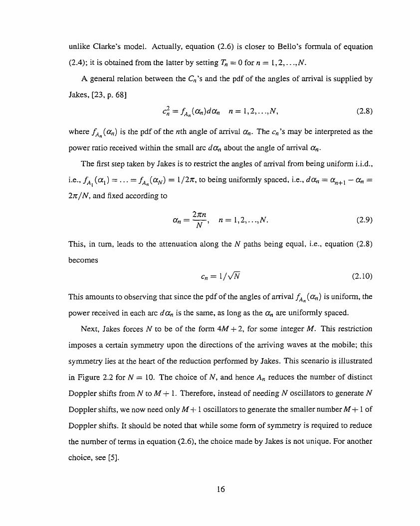
unlike Clarke's model. Actually, equation (2.6) is closer to Bello's formula of equation

(2.4); it is obtained from the latter by setting Tn = O for n = 1,2,. . . ,N.

A general relation between the Ca's and the pdf of the angles of arriva1 is supplied by

Jakes, [23, p. 681

3 = fA,(an)dan n = 1,2 ,..., N , (2.8)

where fA (an) is the pdf of the nth angle of arriva1 an. The c,'s may be interpreted as the

power ratio received within the small arc d a , about the angle of arriva1 cc,.

The first step taken by Jakes is to resvict the angles of arriva1 from being uniform i.i.d.,

Le., fAl (ai) = . . . = fAn (+) = 1 / 2 ~ , to being unifomily spaced, Le., d a n = %+, - a, =

27r/N, and fixed according to

This, in tum, leads to the attenuation dong the N paths being equal, Le., equation (2.8)

becomes

Cn = l / JN (2.10)

This amounts to obseming that since the pdf of the angles of arrival fAn (an) is uniform, the

power received in each arc d a , is the same, as long as the a, are uniforrnly spaced.

Next, Jakes forces N to be of the forrn 4M + 2, for sorne integer M. This restriction

imposes a certain syrnrnetry upon the directions of the arriving waves at the mobile; this

syrnrnetry lies at the hem of the reduction perfomed by Jakes. This scenario is illuswted

in Figure 2.2 for N = 10. The choice of N , and hence A, reduces the nurnber of distinct

Doppler shifts from N to M + 1. Therefore, instead of needing N oscillators to generate N

Doppler shifrs, we now need only M+ 1 oscillaton to generate the smaller number M -t- 1 of

Doppler shifts. It should be noted that while some form of symrnetry is required to reduce

the number of terms in equation (2.6), the choice made by Jakes is not unique. For another

choice, see [SI.

Clarke model N = I O

=

mobile

Jakes' model M = 2

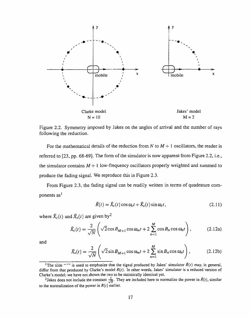
Figure 2.2. Symmetry imposed by Jakes on the angles of arriva1 and the number of rays following the reduction.

For the mathematical details of the reduction from N to M + 1 oscillators, the reader is

referred to [23, pp. 68-69]. The form of the simulator is now apparent from Figure 2.2, Le.,

the sirnulator contains M + I low-frequency oscillators properly weighted and surnmed to

produce the fading signal. We reproduce this in Figure 2.3.

From Figure 2.3, the fading signal c m be readily written in terms of quadrature com-

ponents as1

R(t) = Z ( t ) cosw,t + $ ( t ) sinaCr,

where XJt) and % ( r ) are given by2 M

f icos B ~ + ~ cos w,,t + 2 C cosB, cos ~t n=l

and

' ~ h e tilde "-" is used to emphasize that the signal produced by Jakes' simulator R(r) may, in general, differ from that produced by Clarke's model R(r ) . In other words. Jakes' simulator is a reduced version of CIarke's model; we have not shown the two to be statistically identical yet.

'.Ides does not include the constant 5. They are included here to normalize the power in &t), similar

to the normalization of the power in R ( t ) earlier.

R t )

Figure 2.3. Mes ' fading channel simulator (after [23, p. 701).

where w, is the radian Doppler frequency shifi undergone by the nth arriving wave, and is

given by

The terms cos B, and sinB, are termed oscillator gains; the term is also applied directly

to B,, however. The values for P,l, n = 1,2 , . . ., M + 1 are chosen such that the phase of

the signal R ( t ) is uniformly distributed over [O, 2x1. Iakes points out that there are several

choices for B , , . . ., BM+l. The values chosen by him are

For other sets of values see [23, Figure 1-7-21 or [24, p. 781.

The structure of Figure 2.3 together with the choices made in equation (2.13) is corn-

monly referred to as Jnkes'fnding dznnnel simdntor [5] , [9], [IO], [12], [NI.

A final note on the value of N , or equivalently M. As mentioned before, for large

enough values of N the envelope pdf is Rayleigh. Jakes [23] quotes the works of Slack [20]

and Bennett [21] to justify that a value of M 2 6 is sufficient [23, p. 691. He points out that

deviations from the Rayleigh distribution are confined mostly to the extreme peaks. Other

considerations stemming from, for example, the autocorrelation function, result in other

choices of iV. Jakes indicates that a value of N = 34, or equivalently M = 8, is sufficient

(see [23, p. 691) to assure required accuracy in the autocorrelation function.

2.2.1 A note on the pdf of B,

In this subsection, we determine the relationship between the oscillator gains B l , . . . , BM+

of Jakes' simulator and the phase shifts al,. . ., aN of Clarke's model. We should mention

here that Jakes [23] does not describe how B I , . . ., BM+i are obtained, or how the oscillator

gains of his simulator are related to the phase shifts of Clarke's model.

Re-wnting the signal generated by Jakes' simulator under the constraint that it have

unit power, we have

where we have used the well-known trigonometric identity

cosxcos y i- sinxsin y = cos(x - y).

Substituting another well-known vigonometric identity,

in equation (2.14) yields 7

Recall that R(t) is rneant to be a more efficient realization of R(t ) ,

TO determine the relation between the Bn7s and the On's7 we equate cosines of the sarne

frequency. Recalling that un = CO, cos F7 we have for n = 2M + 1

Similarly, for n = N = 4M + 2, we obtain

from which we infer

- BM+ 1 - -%v+2-

Cornparhg equations (2.16a) and (2.16b)' we must have

From equation (2.17) it follows that Iakes forces = QjM+?; these phase shifts are

no longer independent, as assurned in Clarke's model.

We can obtain a sirnilar result for BI , . . ., BiM. Equating components of equal frequency,

we have

Equation (2.18) may be simplified by combining the two cosines on the left side, i.e.,

Comparing the amplitudes of the cosines in equation (2.19), we have

Equation (2.20) gives an implicit relationship between Q, and Q4M+2-n, for n = 1, . ..,M.

We c m make the relationship between the two phase shifts explicit by observing that they

must satisfj one of the four equalities

for each n = 1,. . .,M. Again, we note that the phase shifts are no longer independent as in

Clarke's model.

Similarly, we may obtain that the phases and @qM+lin must satisQ one of

the four equdities

Retuming to equations (2.191, we now determine the relationship of B , , . . ., BM+ to

@ I , . . . , 0,4M;z. Equating the phases of the two cosines, we have

Substituting equations (2.2 la) - (2.2 id) in equation (2.23) we observe that B I , . . ., BM and

<Pl, . . ., OM must satisfy one of the four equalities

Similarly, we may obtain

and we observe that B, and @,Mil-n mut satisQ one of the four equalities

From equations (2.23) and (2.25), we conclude that the four-tuple of phase shifts a n ,

@ZM+ 1-nt @2Mil+n9 @JM+z-~ for n = 1,. . ., M, are no longer independent as in Clarke's

rnodel.

Returning to equations (2.24a) - (2.24d), we note that BL, . . ., Bhf depend directiy on

<PL,. . .,OM. Aiso, because BI , . . .,(DM are uniform i.i.d. over [0,2n], we conclude that

B , , . . ., BM are also independent and uniformly distributed over some interval of length 2n.

However, since the Bn's appear only as arguments to either cos(.) or sin(-), we may take

the B, as uniform i.i.d. over [O, 2x1 without loss of generality.

2.3 Patzold's analysis

One author who has done extensive research on the topic of deterministic Ming chan-

ne1 simulators is Patzold (see, for exarnple, [7] - [9]). The word cletemzirtistic, as used

by Patzold, is meant to emphasize that the simulator parameters, once chosen, remain un-

changed for the duration of the simulation run. Thus, simulators of the form given in

equation (2.6) fall in this category. In particular, Jakes' simulator is a deterministic model

because once the Cm A,, and B, are chosen they do not change for the duration of the

simulation. We note that this is strictly a choice of nomenclature, and does not affect the

analysis of the model.

Returning to Patzold's work, we note that he has computed the statistics of the Jakes'

fading channel simulator [9]. He obtained analyùcal expressions for the autocorrelation

and cross-correlation functions of the in-phase %(r) and quadrature % ( r ) components, as

well as the envelope and phase pdf's of the resulting fading signal @).

To denve the results mentioned above, Patzold notes that the signal produced by the

sirnulator is deterministic, and thus its properties can be analyzed on the basis of time

averages instead of statistical averages. However, substituting time averages for statistical

averages is meaningful only in the case of (at least) wide-sense stationary and ergodic

signals; Patzold does not veriQ that the fading signal B( t ) possesses either property. It

should be pointed out that in [8] Patzold justifies this approach by observing that for a single

random-phased sine process the time average does indeed equal the statistical average. To

connect this step to the final answer would require the same to be true of sums of such

processes. This is easily shown to be false through the following counterexmple.

Suppose we have the signal

R(t) = cos([ + O) fcos(7t + O),

where O is a random variable uniformly distributed over [O,%]. It is easily shown that

for each of the signais cos(t + 0) and cos(2t + 0) the time average equals the statistical

average. For exarnple, one rnay note that both processes are wide-sense stationary and

ergodic, and hence the two averages are equal. Conversely, one rnay directly compute the

two averages.

Now, we compute the statistical autocorrelation of R(r). It is

E W l M t 2 1 }

= E { [ c o s ( t l + O ) + c o s ( 2 t l i ~ ) ] x [cos(r,+O)+cos(2t2+O)])

= ~ { c o s ( t , + 0 ) c o s ( t ~ + ~ ) ) + ~ { c o s ( t ~ + O ) c o s ( 2 t , + 0 ) )

+ E {cos(2tl +0)cos( t2+O)) i-E {cos(2tl +0)cos(2t2+ O))

Clearly, the statistical average function is not a function of only the time difference t7 - - t l ,

as is obvious from looking at the second term of the sum in equation (2.27).

Next, we compute the time-average autocorrelation of R(t). For a particular value of O,

it is

(R(t)R(t + r))

- - 1 i 5 ~ ~ l - r [cos(t t O) + cos (2r + O)] x [cos(? + 7 + O) + cos(2t + 2~ + a)] dt

Cornparhg equations (2.27) and (2.28), it is clear that the statistical average autocorre-

lation does not equal the time average autocorrelation. Hence, we conclude that, in general,

sums of wide-sense stationary processes may not be wide-sense stationary, thus removing

the possibility that the sum may exhibit any ergodicity properties.

It is also interesting to note that, in general, the statistical autocorrelation is a hinction of

two variables, tl and t, - in our case, while the rime average correlation is a function of only

one variable, usually the time difference r = t2 - r l . In the case of wide-sense stationary

processes the statistical autocorrelation depends only on the time difference r = t2 - t l . It

is no surprise, then, that one prerequisite for equating rime averages with statistical ones

requires the stochastic process to be at least wide-sense stationary.

Furthemore, the computation of the envelope and phase pdf's rests on the assumption

that the in-phase and quadrature components are independent, and thus uncorrelated. In [8],

Patzold notes &(t) and X,(t) are uncorrelated if the sers of frequencies used to generate the

quadrature components are disjoint. With the assumption that the two sets of frequencies

are disjoint, Le., that g(t) and ZJt) are independent, Patzold develops expressions for the

envelope and phase pdf's. He then applies these results to Jakes' simulator in [9]. However,

the assumption required to validate the answer, namely that the two sets of frequencies are

disjoint, is violated. This is readily obvious from [9, eq. (1 l)]. One has to conclude the

results obtained in [9] are unsupported in this sense.

For the sake of completeness, we include below the results derived by Patzold in [9] .

The notation is changed from the original, so that it matches that of this thesis. Also,

3 we set 2% = 1, Le., we normalize the average signal power, much like before when we set

Eo = fi. Another difference from the work presented until now lies in the fact that Patzold

uses lowpass equivalent forms, whereas Jakes uses bandpass forms. The results presented

below also use the lowpass equivalent foms. It should be noted that this is of relevance

only in the case of the autocorrelation and cross-correlation functions. The interested reader

is directed to [9] for details.

The envelope and phase pdf7s of the fading signal R(t) are given by

where,

Note that in order to obtain the enveiope and phase pdf's one has to compute at least double

integrals.

As menrioned above, the time-average autocorrelations and cross-correlation functions

are given in lowpass equivalent fom. To obtain the corresponding bandpass forms, such

as those used by Jakes, muluply the equations below by cos(&t). In the limit, as N be-

cornes large, the time-average lowpass equivalent in-phase and quadrature autocorrelation

functions are, respectively,

and

where the superscript LP is used to emphasize we are using lowpass equivalent forms.

Patzold notes that neither of these time-average autocorrelations matches the desired, sta-

tistical one, i.e.,

However, the time-average autocorrelation function of the complex Gaussian fading sig-

nal, given by the sum of the time-average autocorrelations of the in-phase and quadrature

cornponents, matches the expected one, i.e.,

The time-average autocorrelations given in equations (2.29a) and (2.29b) hold m e only in

the lirnit, as N cl.. For finite N, the reader is directed to [9]. However, it is worthwhile

mentioning that in this case the time-average autocorrelation of the fading signal (R(t)l?(t + ~ j ) matches the expected autocorrelation closely over the interval [O, (M + L)/(2Jn)] only.

Ln [93, the expression for the time-average cross-correlation of the in-phase and quadra-

ture components is left in integral form,

(Xs(t)Zc(t + T) j Lp - sin(&) cos(m,,r cos z)dz.

Note that in general the time-average cross-correiation is non-zero.

Patzold concludes that lakes7 approach is usehl in the design of fading channel simu-

lators. In fact, he uses this approach to denve a number of similar simulators. The structure

is essentially the same for al1 of the models derived. The differences lay in the rnethod

chosen to compute the simulator parameten, such as the path attenuation coefficients C,,

the radian Doppier frequency shifts Cln = CO SA^, and the phase shifts a,. For these

other types of simulators, the reader is referred to [7] and [8]. However, the conclusions

drawn herein will apply equally to ail simulators derived by Patzold, with perhaps minor

modifications.

2.4 Problems with the simulator

Despite the simplicity and widespread use of Jakes' simulator, there are some drawbacks

to its employ. We point out below some of the problems inherent in the simulator.

A potentially serious problem lies in the assumption that the fading signal produced

by Jakes' simulator is wide-sense stationary. Gilbert [2] noted that choosing the N phases

independently from a uniforrn distribution over [O, 2x1 for the N arriving waves, leads to

models generating wide-sense stationary signals. Cenainly, in equation (2.6) this condition

is met. However, this condition is not readily verified by analyzing Figure 2.3.

Another drawback to Jakes' simulator is that there is no obvious relationship between

the gains B , , . . ., BM, and the pararneters of the model of equation (2.6), in particular the

phase shifts an, n = 1,. . ., N. One of the advantages of the model of equation (2.6) is that

it relates in a straightfonvard manner to the physical world. This obvious relationship is

lost in the denvation leading to lakes' simulator. Note that we have already addressed this

problem in Section 2.2.1.

An inherent drawback to fading channel models is that signals generated based on them

are only approximations to the fading phenornena observed over mobile radio channels.

The obvious analogy is that just as representing an analog signal by a digital one introduces

quantization errors, so simulation in our case inrroduces errors. These errors a i se from

the resolution of the continuum of paths present between trammitter and receiver into N

waves. There has been some work done in uying to estirnate the errors introduced by this

quantization process, most notably that of Patzold et al. [7], Patzold et ai. [8], and Patzold

et al. [9]. Conversely, one might be interested in how many low-frequency oscillators one

needs in an implementation, software or hardware, to reduce the error to an acceptable

level. Many authors have provided unsubstantiated answers to this question; for example,

Jakes [23] suggests that more than 6 oscillators are sufficient, while Patzold [9] suggests

that 10 are enough. However, when modelling channels some authors resort to using a

much higher number; for example Hoeher [12] uses 500. We need some means of relating

the error introduced during the quantization process to the number of oscillators used in the

simulator.

Finally, two important properties which may be used to advantage by the wireless en-

gineer are stationarity and ergodicity. While there is littie known about whether flat fading

channels are indeed ergodic, some rnodels do exhibit this property. A useful property

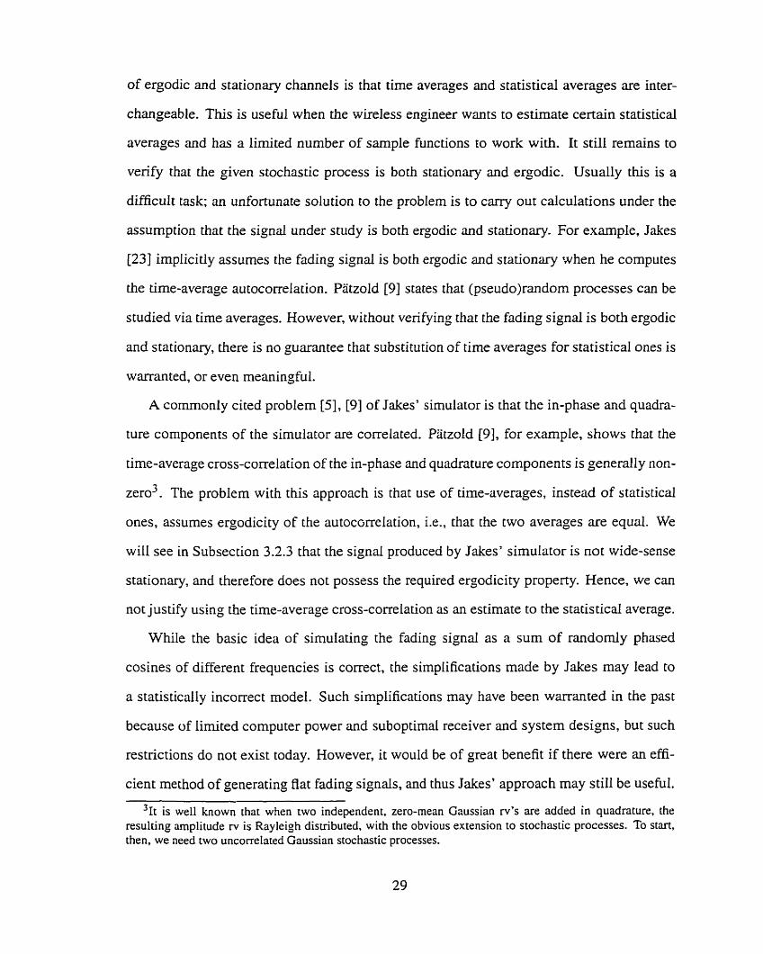
of ergodic and stationary channels is that time averages and statistical averages are inter-

changeable. This is useful when the wireless engineer wants to estimate certain statistical

averages and has a limited number of sample functions to work with. It still rernains to

verify that the given stochastic process is both stationary and ergodic. Usually this is a

difficult task; an unfortunate solution to the problem is to carry out calculations under the

assumption that the signal under study is both ergodic and stationary. For example, Jakes

[23] irnplicitly assumes the fading signai is both ergodic and stationary when he computes

the time-average autocorrelation. Patzold [9] States that (pseudo)random processes c m be

studied via time averages. However, without veriming that the fading signal is both ergodic

and stationary, there is no guarantee that substitution of tirne averages for statistical ones is

warranied, or even meaningful.

A comrnonly cited problem [SI, [9] of Jakes' simulator is that the in-phase and quadra-

ture components of the simulator are correlated. Patzold [9] , for exarnple, shows that the

time-average cross-correlation of the in-phase and quadrature components is generally non-

zero3. The problem with this approach is that use of tirne-averages, instead of statistical

ones, assumes ergodicity of the autoc~rrelation, i.e., that the two averages are equal. We

will see in Subsection 3.2.3 that the signal produced by lakes' simulator is not wide-sense

stationary, and therefore does not possess the required ergodicity property. Hence, we can

not justib using the time-average cross-correlation as an estimate to the statistical average.

While the basic idea of simulating the fading signal as a sum of randomly phased

cosines of different frequencies is correct, the simplifications made by Jakes may lead to

a statistically incorrect model. Such simplifications may have been warranted in the past

because of limited computer power and suboptimal receiver and system designs, but such

restrictions do not exist today. However, it would be of great benefit if there were an effi-

cient method of generating flat fading signals, and thus Jakes' approach may still be useful.

3 ~ t is well known that when two independent, zero-mean Gaussian rv's are added in quadrature. the resulting amplitude rv is Rayleigh disuibuted, with the obvious extension to stochastic processes. To start, then, we need two uncorrelated Gaussian stochastic processes.

To this end, this thesis tries to answer the question of whether the number of oscillators c m

be reduced from N, while still generating a statistically correct fading signal.

Chapter 3

S tatistical Properties of Sum-of-Sinusoids Simulators

In this chapter, we analyze the statistical properties of sum-of-sinusoids simuiators, of

which Jakes' simulator is a special case. We start with the development of some theory

relating to the computation of the pdf of the sum of independent random vectors. We then

use the results to compute the pdf's of the envelope of the signal generated by Clarke's

mode1 and of the envelope of the signal generated by Jakes' simulator. As well, we obtain

the phase pdf's in the two cases mentioned above. We continue by computing the auto-

correlation hnction of each of the two signals. It will be shown that while the signal of

equation (2.6) is at ieast wide-sense stationary, the signal produced by lakes' simulator is

not. We conclude the chapter with a discussion of the ergodic properties of the signals

generated by Clarke's mode1 and f &es' simulator.

3.1 First-order statistics

In this section, we develop some theory to be used in the calculation of the envelope and

phase pdf's of the signals produced by sum-of-sinusoids simulators. The approach most

often followed when computing these pdf's is to observe that the fading signal can be writ-

ten in terms of quadrature terms, as in equation (2.1 1). Each of the in-phase and quadrature

terms is shown to be approximately a zero-mean Gaussian random process; hence the en-

velope resulting after combining the two independent random processes in quadrature will

be approximately Rayleigh distributed. There is a considerable body of literature relating

to the computation of the pdf resulting from adding randornly-phased sine waves. See, for

example, the works of Slack [20] and Bennett [21]. As well, Rice has contributed through

his classical papers [14] and [ 151, as well as [16] and [ 181. More recently, see the works of

Patzold [8] and Helstrom [19].

There are very few results pertaining to the direct computation of the envelope and

phase pdf's. One such result is presented by Goldman [17]. However, he does not present

a proof of the result. Here we give a simple proof, hoping to gain additionai insight into

the problern. We attempt to soive the problern by noting we are adding independent two-

dimensional random variables. We already know that the pdf of the sum of independent

(scalar) randorn variables c m be obtained by the convolution of the pdf's of the randorn

variables. In the Fourier transform domain, this amounts to multiplying the characteristic

functions of the random variables. The pdf of the surn is then obtained by taking the inverse

Fourier transform of the product of characteristic functions. A sirnilar approach is followed

here.

We denote the nth random vector in the sum by (X,, Y,), for n = 1, . . . , N. Here, we may

interpret (X,l, Y,) as a vector in the plane, with Xn the increment in position along the x-axis

and Y, the increment in position along the y-axis. In general, Xn and Y, are correlated.

Altematively, we could use polar coordinates (Rn, O,) to represent the sarne random

vector. In this case, Rn can be interpreted as a length, while O, as a direction measured

from the positive x-axis.

In what follows, we assume Rn is independent of O,; this is saying precisely that the

length of the random vector bears no relation to its direction. When applying the results

obtained herein, we rnust make sure that the above assumption is justified; this justification

may be provided by the nature of the problem. Moreover, the pdf's of Rn and en are

easily obtainable from the description of the problem. In panicular, when al1 directions are

equally likely, the angle pdf is

The independence of Rn and 0, will make it much easier to work in polar coordinates.

Observe that the N random vectors (X,, YI ), . . ., ( X N , Yy) or (RI, el), . . ., ( R N , ON) are in-

dependent of each other; the representation, Cartesian or polar, is irrelevant.

Geometrically, we are interested in determining the joint probability density function

(jpdf) of the resultant vector sürn, Le., the jpdf of the length and direction from the positive

x-axis. Ultimately, however, we want to determine the pdf of the magnitude of the sum R

of the N random vectors, and the pdf of the angle O the final point rnakes with the positive

x-axis. Le., the pdf's of the random variables'

R = dx2+Y2 and O=arctan(X,Y),

where X and Y are defined by

and

We assumed above that Rn and 0, are indepenaent. It is not obvious from this assumption

that R and O are also independent; we will see that they are indeed independent below.

Figure 3.1 and Figure 3.2 illustrate the summation process with one, and two random

vectors, respectively. For the purposes of illustration, we have restricted Rn = 1. The circles

represent the sets of reachable points after one and two steps, respectively, i-e., one can not

reach the shaded area.

The technique we will be using to arrive at the desired answer is outlined next. As

mentioned above, the vectors being added are independent. Therefore the characteristic

'The arctan(.r, y) function returns the proper angle, Le., indudes quadrantal information.

Figure 3.1. First step in summing two-dimensionai independent random vectors of unit length. Note that only points on the unit circle can be reached.

Figure 3.2. First two steps in summing two-dimensional independent random vectors of unit length.

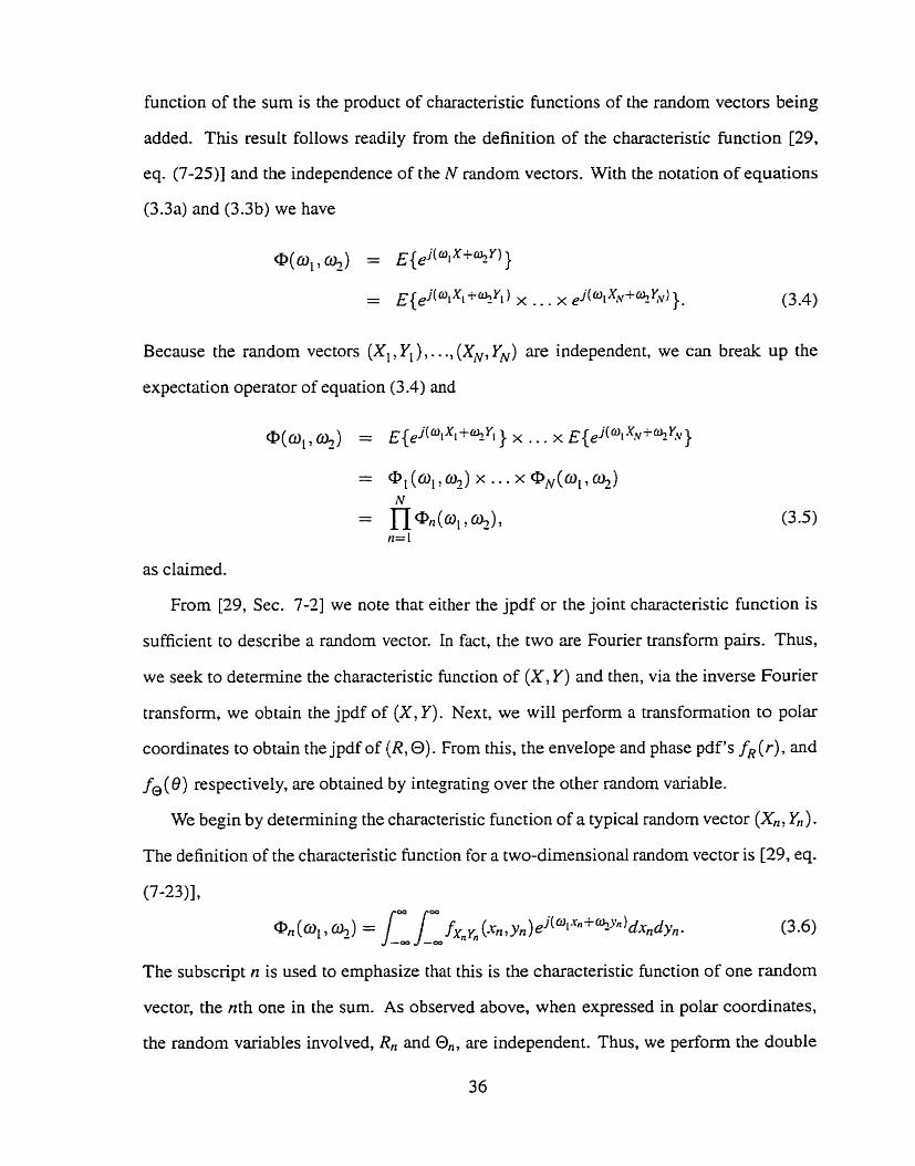
function of the sum is the product of characteristic functions of the random vectors being

added. This result follows readily from the definition of the characteristic function [29,

eq. (7-25)] and the independence of the N random vectors. With the notation of equations

(3.3a) and (3.3b) we have

Because the random vecton (X,, Y l ) , . . ., (Xlv) YN) are independent, we can break up the

expectation operator of equation (3.4) and

as claimed.

From 129, Sec. 7-21 we note that either the jpdf or the joint characteristic function is

sufficient to describe a random vector. In fact, the two are Fourier transforrn pairs. Thus,

we seek to determine the characteristic function of (X, Y) and then, via the inverse Fourier

transform, we obtain the jpdf of (X, Y). Next, we will perform a transformation to polar

coordinates to obtain the jpdf of (R, O). From this, the envelope and phase pdf's f&), and

fo(8) respectively, are obtained by intepting over the other random variable.

We begin by determining the characteristic function of a typical random vector (X,, Y,).

The definition of the characteristic function for a two-dimensional random vector is [29, eq.

The subscript n is used to emphasize that this is the characteristic function of one random

vector, the nth one in the sum. As observed above, when expressed in polar coordinates,

the random variables involved, R,, and CDn, are independent. Thus, we perform the double

integration in (3.6) by converting to polar coordinates. To perform the change of variables

we use [29, eq. (6-72)]

Performing the change to polar coordinates in equation (3.6) yields

Next, we use the independence of R, and 0, to separate the jpdf fRnOn (rn, %), and obtain

where y, = arctan(ol, CO,). - To evaluate the integral inside the square brackets, we use [36,

eq. 8.4 1 1.71 to obtain the equality

Performing the substitution B =

we obtain

8, - y, in equation (3 -9) and using equation (3.1 O),

Observe that the characteristic function of equation (3.1 1) is circularly syrnrnecric, i-e.,

it depends only on the length of the vector (al, a,). - Integais of the form of equation

(3.111, i.e., in which we integrate against the Bessel function JO(-), are referred to in the

literature as Hankel transforms. The Hankel transform is useful in other areas of study, such

as optics, in which circular symmetry is inherent. For more on two-dimensional Fourier

transforms and the Hankel transform see [3512.

? ~ h i s would be useful in the event oqe wanted to perform the integration of equation (3.1 1); [35] contains a table of HankeI transforms.

We are now in a position to compute

dent random vectors

Substituting equation (3.1 1) in equation

N

the characteristic function of the sum of indepen-

(3.5) yields

To obtain the jpdf of (X, Y ) we take the inverse Fourier transform of @(ml , u,) accord-

ing to [29, eq. (7-24)]

We choose to perforrn the double integration of equation (3.14) by changing to polar

coordinates

o l = q c o s e , -=qs ine .

Substituting equation (3.15) in equation (3.14), yields

where = arctan(x, y). The negative sign in the exponential may be absorbed by the cosine

via a shift of n. We now use equation (3.10) to evaiuate the integral in the right set of square

brackets. We thus have

Next, we convert the jpdf of equation (3.17) to polar coordinates to obtain the jpdf of

the random vector (R, O). Letting

in equation (3.17) and substituting in equation (3.7) @es

Note that we can separate the jpdf of R and O as

proving that, indeed, R and O are independent random variables. Furthermore, fR& 6)

in equation (3.19) does not depend on 0. From this we conclude that O is uniformly

distributed over [O, 2x1

regardless of the number N of random vecton added.

To obtain the pdf of the magnitude of the sum of N random vectors fR(r) , we may

integrate the jpdf f,,(r, 8) over the variable 8. Integrating equation (3.19) with respect to

O, we obtain

For the purpose of illustration, we show how to use equation (3.22) in a simple case.

We restrict Rn = dm, i.e., a deterministic pdf as in Figure 3.1 and Figure 3.2. The pdf

corresponding to this choice is

where 6(9 is the Dirac delta function. The random vector length is normalized such that

the variance of the rv's X and Y is always one.

Note that other choices of fR (r,) are possible, depending on the problem at hand. We

chose the pdf of equation (3.23) as this provides the simplesr answers. For other applica-

tions, such as modelling hardware errors, the lengths rnight follow a uniform distribution

over some interval [a, b] , or Gaussian, whichever is a better rnodel. One could then com-

pute the pdf of R to detemine whether errors in the hardware will have an effect on the

generation of Rayleigh distributed random variables, Le., Rayleigh fading signal.

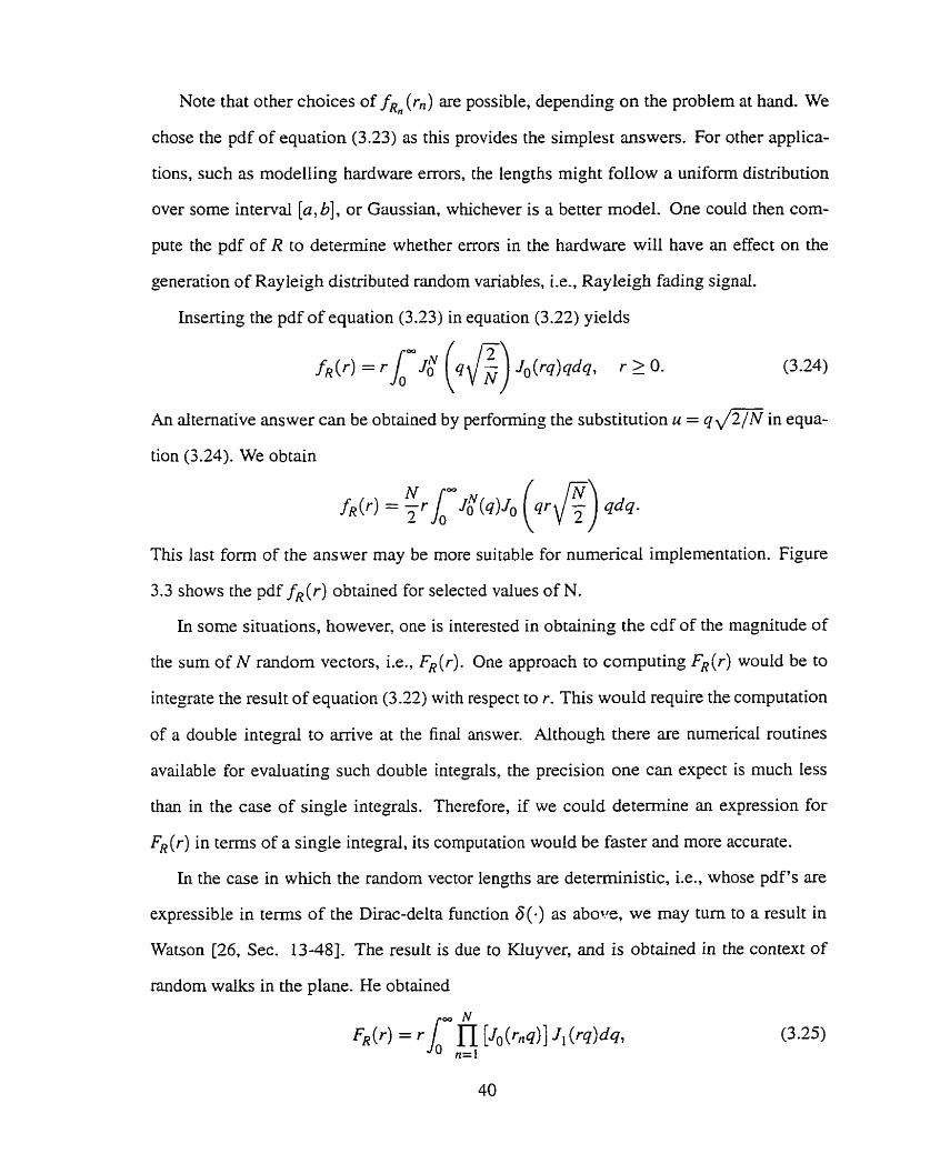
Inserting the pdf of equation (3.23) in equation (3.22) yields

An alternative answer can be obtained by perforrning the substitution u = q J ~ / N in equa-

tion (3.24). We obtain

This last f o m of the answer may be more suitable for nurnencal implementation. Figure

3.3 shows the pdf f,(r) obtained for selected values of N.

Zn some situations, however, one is interested in obtaining the cdf of the magnitude of

the sum of N random vectors, i.e., FR ( r ) . One approach to computing FR ( r ) would be to

integrate the result of equation (3.22) with respect to r. This would require the computation

of a double integrai to arrive at the final answer. Although there are numencai routines

available for evaluating such double integrals, the precision one can expect is much less

than in the case of single integrals. Therefore, if we could deterrnine an expression for

FR(r) in terms of a single integrai, its computation wouid be faster and more accurate.

In the case in which the random vector lengths are detemiinistic, Le., whose pdf's are

expressible in terms of the Dirac-delta function 6(9 as abo~re, we may tum to a result in

Watson [26, Sec. 13-48]. The result is due to Kluyver, and is obtained in the context of

random wallcs in the plane. He obtained

Figure 3.3. Envelope pdf of the signal generated by Clarke's mode1 for various numbers of low-frequency oscillators.

where the rn represent the lengths of the individual steps. It should be noted that such a

case does occur; Clarke's model with constant cn7s would be an irnrnediate exmple. The

result of equation (3.25) is used later, in Section 5.1.

Unfortunately, there seems to be no such resuIt in the more general case, where the Rn

are ailowed to follow any distribution. For these cases we are forced to perform the double

integration as mentioned above.

3.1.1 The envelope and phase pdf's of Clarke's model

We presented in Section 3.1 a method for computing the jpdf of the random vector repre-

senting the sum of N independent random vectors in the plane. Here we will apply this

method to compute the envelope and phase pdf's of the signal produced by Clarke's model.

Of course, to be able to apply the results of Section 3.1, we must first recast the problem

in terms of a surn of independent vectors, i.e., in the form of equations (3.3a) and (3.3b).

Also, we must justify the assumption that R,, and 0, are independent. In addition, we must

venfy that the On's follow the pdf of equation (3.1).

Recall that we are trying to simuiate the fading signal of equation (2.6). Here, we

re-write this signai split into in-phase and quadrature components,

R(t) = cos w,t cos(ant + a,,) - sin w,r (3 -26) n= 1 n= l

By cornparing equation (3.26) to equations (3.3a) and (3.3b), we note,

and

@ n = ~ l i t + @ n , n = l , ..., N. (3 -28)

To justify the independence of Rn and 0, we turn to the model of equation (2.6). In

this equation, the parameters C,, A,, and CDn are al1 independent. From equation (3.27) we

30ne may also note that Rn constant is sufficient to guarantee R, and O,, are independent.

43

note Rn is a function of Cn only. From equation (3.28) we note 0, is, in generd, a function

of An and 9. From the independence of C,, An, and a,, it follows that Rn and 0, are also

independent.

From equation (3.27), the length pdf of the izth random vector is given by the pdf of

equation (3.23), Le.,

In equation (3.28) we have a detenilinistic component w,r and a random one an. Therefore,

the pdf of On will be the sarne as that of an, except that it will be shifted by an arnount equal

to ant. Recall that the pdf of a, is uniform over some interval of length 2x. However, due

to the penodicity of the functions involved, Le., cos(-) and sin(.), this is sufficient and we

may take the 0,, to be uniform i.i.d. over [O, 2x1. This satisfies the requirement of eqoation

(3.1). We now proceed with the cornputation of the envelope pdf of the signal produced by

Clarke's rnodel.

To determine the envelope pdf, we need to substitute the appropriate pdf fR.(rlr) in

equation (3.22). We note the required result appears in the worked exarnple at the end of

Section 3.1. From equation (3.24), we have

We note that the envelope pdf of the signai produced by Clarke's mode1 is independent of

time t. We plot the result in Figure 3.4.

The phase pdf is given by equation (3.2 1)

1 f@(e) = Z;; for O 5 8 5 2 ~ .

3.1.2 The envelope and phase pdf's of Jakes' sirnuiatm

In this subsection, we determine the envelope and phase pdf7s of the signal produced by

Jakes' simulator.

Figure 3.4. Variation with time of the envelope pdf of the signal produced by Clarke's model, for N = 34.

As in the case of Clarke's model, Our first task is to recast the fading signal produced by

Jakes' simulator in tems of the sum of M + 1 independent random variables. We re-write

the signal of equation (2.11) in tems of quadrature components

Sirnilar to the procedure in the previous section, we compare equation (3.3 1) to equations

(3.3a) and (3.3b). We see that the random vector lengths are described by the random

variables

2\/2 - - R,,, - JN cos @t,J.

The corresponding randorn vector directions are described by the random variables

As done in the previous section, we must first verify that R,, is independent of O,. We note

that Rn is, in general, a function of Cn and A,. O,, on the other hand, is a function of Bn, and

hence, <Pn only. We have already argued that Cn, A,, and QI are independent from physical

considerations in Section 2.1. It follows, then, that Rn and 0, are also independent.

From equation (3.32), the pdf's of the random vector lengths are given by

and

Recall from Subsection 2.2.1 that we may take the rv's B I , . . ., BM+1 unifonn i.i.d. over

[O, 2x1. Thus, the rv's QI , . . ., are uniform i.i.d. over [O, 2x1, satiswing equation (3.1).

Thus, substituting equations (3.34a) and (3.34b) in equation (3.11) yields

and

Next, following a procedure similar to that in Section 3.1 we obtain

We note that the pdf of the envelope of the signal produced by Jakes' simulator is a fûnction

of both the envelope levei r as well as tirne t. We plot the result of equation (3.36) in Figure

3.5. Analyzing Figure 3.5 we note that the variance of the failkg process is time-variant.

That is, the signal produced by Jakes' simulator is not stationary, nor even wide-sense

stationary. The non-stationary character of the signal will be observed in a different form

in Section 3.2.2.

The phase pdf is given by equation (3.2 1)

L f6(@) = for O 2 0 < 2x. (3.37)

It is interesting to note that this result contradicts Patzold's development in [9 ] . Patzold

derives his resuics based on time averages. Here, we have computed a statistical average.

We have also shown that the first-order pdf of R(t) is time-variant, and thus suspect the

random process I?(t) is not wide-sense stationary; we will show this directly later. This

point further illustrates that one may not readily substitute tirne averages for statistical ones;

such substitutions are meaningful only for randorn processes which satisQ some ergodic

theorem, i.e., which exhibit ergodicity of the mean and autocorrelation.

3.2 Second order statistics

In this section, we compute the statistical mean and autocorrelation functions of the sig-

n a l ~ produced by Clarke's mode1 and Jakes' simulator. We find that the signal produced

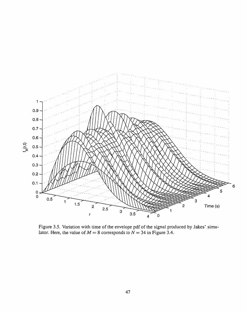
Figure 3.5. Variation with time of the envelope pdf of the signal produced by Jakes' simu- lator. Here, the value of M = 8 corresponds to N = 34 in Figure 3.4.

by Clarke's model is wide-sense stationary, while that produced by Jakes' sirnulator is not

wide-sense stationay As well, we determine the tirne-average mean and autocorrelation

functions. These computations are readily carried out from appropriate definitions of the

mean and autocorrelation functions. Cornparisons of the two sets of averapes, Le., statisti-

cal and time-average, are made in the general frarnework of egodicity. We 'end that in the

case of Clarke's model, the statistical mean and autocorrelation functions are equal to the

corresponding time-average functions. In the case of Jakes' model, this is me of only the

mean function.

3.2.1 Clarke's rnodel

In this subsection, we determine the autocorrelation BRR ( r l , r2) of the stochastic process

R(t ) represented in equation (2.6), a second order statisticd property. For the sake of

completeness, we also compute the mean function pR (1). Recdl that the fading signal R(t )

c m be written as

where o, = ~ c o s ( Z n n / N ) . This re-formulation is equation (2.6) with the c, and a, as

given by equations (2.9) and (2.10) in Section 2.2. In other words, the only rv's are the 4,

which we recall are uniform i.i.d. over [O, 2x1. This simplifies the cornputation of the mean

and autocorrelation functions of the fading signal R(t ) .

Applying the definition of the mean function as defined in [29, eq. (10-7)], we obtain

successively

where we have used the linearity of the expectation operator, and the fact that the integrai

of a sine wave over one wavelength is zero.

To compute the autocorrelation function, we also start from the definition 129, eq. (10-

8)]. We obtain successively

The first line in the development of equation (3.40) cornes from substituting the definition

of R( t ) . To obtain the next line, we use the well-known trigonometric identity,

Taking advantage of the fact the an are uniform i.i.d. rv's over [O, 2x1 we obtain the fol-

lowing results,

O i f n f k , E {COS (an - ak) ) 1 i f n = k,

This allows us to further simplify equation (3.40) to

We observe that upon expanding cos[oc(tl - t?) + W, ( t l - t2) COS F] we should have two

quadrature terrns. The in-phase one corresponds to cos(oCt), while the quadrature one

corresponds to sin(o,t). We observe, however, that for N even

To prove the result of equation (3.43), we observe that

~ K ( $ + R ) COS

N = COS ( x + F)

Therefore,

uh, (tl - t2) COS N - - t,) cos -

N

For N even, we cm re-write the surnrnation of equation (3.43) as

= y sin [a,,(tl - t2) COS - N

~, , ( t , - tî) cos - 2 1 1 ( B f n i ] . (3.46) n= 1 N

Upon substitution of equation (3.45) in equation (3.46), the result of equation (3.43) is

obvious.

For N odd, the approximation

holds true for O 5 o,(t , - t2) 5 F. This result can be verified graphically, or by using a

method introduced later in Section 5.2.

Thus, in general, equation (3.42) can be approximated by

for O 5 rl - t2 5 &. It should be noted that most sum-of-sinusoids simulators use an even

number of oscillators N, and thus the approximation of equation (3.48), with no restriction

on r , - t2, becornes exact.

As an aide, we relax the assumption that the cc,, n = 1, . . ., N are uniforrnly spaced

around the unit circle, as in Section 2.2. However, we still maintain that the An are uniforrn

i.i.d. random variables over [O, 7x1. Furthemore, the A, are independent of the Qn, as

assumed by Clarke [3] and Jakes [23], for exarnple. This assumption seems physically

reasonable as it States that the phase shift is independent of the angle of mival . Recall

that the angle of arriva1 is affected by the pcsition of the obstacles between transrnitter and

receiver, whereas the phase shift depends on the material characteristics of the obstacles.

Because of the independence of the two sets of rv's, the statistics computed thus far still

apply; we only need to average the results obtained over the pdf of A,. Thus, we still have

We tum Our attention now to the re-computation of the autocorrelation function. We

know from Gans [4] that the power spectral densityhof the fading signal of equation (2.6)

is given by

3 ~ ; 2 S ( 0 ) = - , oc - a,,, < o < oc + a,, - (3.49)

2 JO;~-(W-COJ'

The autocorrelation of the signal can then be computed by taking the inverse Fourier trans-

form of the power spectral density S ( o ) ,

In Our case, Eo = fi, and equation (3.50) simplifies to

Here we present a time-domain derivation, starting with the fading signal R(t) as given

in equation (3.38). Because A, and 9 are independent, the derivation is identical to that

'This dso appears in Jakes [23, eq. ( 1.2- 1 111.

presented above. We pick things up at equation (3.42). At this point, we have to average

the expression of equation (3.42) over the pdf of A,. Thus,

where we have used the well-known trigonornetric identity

cos (x + y) = cos xcos y - sinxsiny.

As well, we have moved the deterministic factors cos w,t and sin o,t outside the expectation

operator.

The next step is to compute the expectations in equation (3.52) as appropriate integrals

From [36, eq. 3.7 15-13] with n = O we have

Thus, substituting equation (3.10) and equation (3.54) in equation (3.53) yields the desired

answer, narnely

g R R ( t l , t2) = c0s[ac(ti - t 2 ) ]J0 (~ tn ( t l - t2) ) . (3.55)

We note that the fading process defined in equation (2.6) is indeed wide-sense station-

ary, so that we may write

g R ( 5 ) = COS(W,~)J~(O,,T). (3.56)

The result of equation (3.56) is the same as that of equation (3.5 l), except for a factor of 3

in the latter. This difference occurs because in Gans' work, the effect, Le., the gain, of the

Figure 3.6. Lowpass equivalent form of the autocorrelation function of R( t ) , for N = 34, w,, = 1.

antenna is also included. As it happens, the gain of an omnidirectional antenna, the type

used by Gans in his analysis, is 3. Also, inclusion of both negative and positive frequencies

introduces a factor of two. We conclude, then, that the two results are identical up to the

inclusion of antenna gains.

A plot of the lowpass equivaient form of the autocorrelation function given by equation

(3.42) is shown in Figure 3.6. From this diagram, the independence of the autocorrelation

function of time origin is obvious. In particular, the surface can be readily obtained by

translating a slice parailel to either axis dong the line t , = t2. This is generally true of

wide-sense stationary processes.

3.2.2 Non-stationarity of Jakes' simulator

In this subsection, we compute the autocorrelation function g R R ( t i ,t2) of the signai pro-

duced by Jakes' fading channel simulator R(r) , a second order statistical property. As well,

we compute the mean function pR( t ) of R(t) , paralleling the developments of the previous

subsection.

For ease of reference, we copy equations (2.11) of Section 2.2 here

where the in-phase and quadrature cornponents. xc(t) and % ( t ) are piven by equations

(2.12a) and (2.12b)

We recall that the purpose of Jakes' fading channel simulator is to efficiently generate the

fading signal of equation (2.6)

We begin with the computation of the mean function pR (t). From Subsection 2.2.1, we

have that B I , . . ., BM+ are uniform i.i.d. over [O, 2x1. Knowledge of these pdf's allows us

to cornpute the expectations

We c m now compute

Sirnilarly, we obtain E{&(t)) = O. Therefore,

To make the derivation of the autocorrelation function simpler, we re-write the signal

produced by the Jakes' simulator by expanding the expressions for the quadrature terms.

That is,

cos B, cos w,t

2&

+ (x sin BLWil cos OJ,J + - sin Bn cos an[ JN ,=i

2 a +- 4 M

fi sinBlw+ cos alnt sin wcr + - sin B, cos &t sin aCt . (3.63)

f i n = [

We can funher simpliQ equation (3.63) by grouping the deterministic terms and making

the substitutions

cos &t cos WC[ = aM+ ( t ) > (3.64a)

and

cos ~ù,,,t sin uCt = bIMi ( f ) ,

Substituting equations (3.64a) - (3.64d) in equation (3.63) yields

Next, we determine the autocorrelation hnction according to the definition [39, eq.

(10-8)]. We have

To simplify the result of equation (3.66) we use the linearity of the expectation operator to

move it inside the summation signs. To further simplify the result of equation (3.66) we

make use of the following equalities, readily obtainable by noting that the rv's B I , . . ., BM+1

axe uniform i.i.d. over [O, 2x1. This allows us to Cornpute

2, i f n = k , E {cos B, cos Bk} = E {sin& sin Bk) = 0, otherwise,

for 1 5 n, k 4 M + 1. Thus, we may simpliQ equation (3.66) to

Back-substituting equations (3.64a) - (3.64d) in equation (3.67) yields

8 bf

+ - (COS Untl COS Uctl COS Unt2 COS Qt, + COS OrIf, sin mCtl COS ont2 sin O&) . N n= 1

We now use the well-known trigonometric identity

cos(x - y) = cosxcosy + sinxsiny

in equation (3.68) to obtain

COS

We c m re-write the autocorrelation obtained above in a slightly different form, by using

the trigonometric identity of equation (3.41), to obtain

Note that

Figure 3.7. Lowpass equivalent f o m of the autocorrelation function of R(t), for M = 8 corresponding to N = 34 in Figure 3.6, and o, = 1.

as N -+ =, or equivalently M -+ =, where we have used 123, eq. (1.7-IO)] to detennine

the limit of the sum. That is, the variance of the stochastic process R(t) is time-variant, as

already observed in Subsection 3 - 1 2

A plot of the lowpass equivalent form of the autocorrelation function produced by

Jakes' simulator is given in Figure 3.7. Upon comparing Figure 3.6 and Figure 3.7, the

non-stationary character of the signal produced by Jakes' simulator is readily obvious. In

particular, note that unlike the autocorrelation of Figure 3.6, the autocorrelation depicted in

Figure 3.7 does not exhibit translational invariance dong the line tl = t2.

Furthemore, the form of equation (3.70) emphasizes the dependence of the autocor-

relation fùnction of the signai generated by Jakes' simulator R(t ) on both the difference

t2 - t , and the sum t, + t , . From this, we are forced to conclude the signal produced by

Jakes' simulator is not stationary. Indeed, it is not even wide-sense stationary. Observe that

the signal will, in general, not be cyclostationary either, as the frequencies in the fading

signal R(t ) are incornmensurate.

3.2.3 Ergodicity of the fading signal

In this section we analyze some of Patzold's work and determine whether the fd ing sig-

nais produced by Clarke's mode1 and Jakes' simulator possess ergodicity of the mean and

autocorrelation.

A comrnon problem facing the wireless engineer is that of estimating some statistic, Le.,

average, of a stochastic process given a small number, usually one, of sarnple functions. In

other words, one uses time averages to estimate statisticai ones. In pmicular, it is of interest

to know when time averages are equal to corresponding statistical averages; this is the topic

of ergodic theorems [32], [33].

A theorem due to Birkhoff and Khinchin [33, p. 1771 States that for ergodic and station-

ary stochasric processes the sarnple, i.e., time, averages converge to the statisticd averages

with probability one. The difficulty in applying this theorem lies in the verification of the

ergodicity and stationarity properties. It would seem appropriate that stationarity, in some

sense, is required to apply this theorem, and in general, ergodic theorems. That is, averag-

ing over time removes dependence on a time origin. Similarly, the statistics of stationary

stochastic processes do not depend on time oripin. The ergodicity property is required to

ensure that al1 convergent samples, Le., time, averages converge to a constant and not to a

random variable.

Due to the technical difficulties5 encountered in the verification of the ergodicity and

' ~ r ~ u r n e n t s about the ergodiciry and stationarity of processes are most easily handkd via measure theory. For an excellent treatment of the subject, though outside the scope of this thesis, the reader is directed to [32].

59

stationarity properties, the wireless engineer is forced to resort to weaker requirements,

such as wide-sense stationarity instead of strict stationarity. Correspondingly, the state-

ments one would be able to make would be weaker. Another common approach, often

followed in elecrrical engineering fields, is to classify stochastic processes as possessing

ergodicity of nth order if the nth order tirne average is equal to the nth order statistical

average in some sense. For exarnple, stochastic processes whose sarnple, time-average,

mean is equal to the statisticd mean are said to possess ergodicity of the mean. Sirnilarly,

stochastic processes whose sarnple, time-average, autocorrelation is equal to the statistical

autocorrelation are said to possess ergodicity of the autocorrelation.

In this simpler case, conditions exist which help one determine whether a signal pos-

sesses either type of ergodicity. Slutsky's theorem [29, p. 4301, for exarnple, states that

for wide-sense stationary processes, ergodicity of the mean is guaranteed if the autocor-

relation function is bounded and its average value tends to zero. Unfortunately, simple

conditions under which ergodicity of the autocorrelation exists are not given; usually, this

requires knowledge of fourth-order statistics. In the case of normal processes, however,

knowledge of the autocorrelation function is sufficient. This usually mems that one has to

cornpute both the statistical autocorrelation and the time-average one to determine whether

they are equal. We still need to determine in what sense the time-average autocorrelation

converges to the statistical autocorrelation, i.e., we may need to determine the variance of

this estimator if its use is to be of my relevance.

Unfortunately, cornmon practice arnong some wireless engineers is to assume a given

stochastic process, such as that representing a multipath fading signal, is both stationary

and ergodic. This assumption then serves as justification for replacing statistical averages

by time averages. The flaw in rhis approach is illustrared by Jakes [23] and later by Patzold

[9]. The latter author states that pseudo-random processes can be studied on the basis of

time averages providing no explmation why this approach might work. We have already

Also, an excelIent inuoductory text is [33].

60

shown the signal of Jakes' sirnulator to be not wide-sense stationary. As such. we would

not expect to be able to make any staternents about the statistical autocorrelation of the

signal produced by the simulator based on a single sarnple signal.

We begin by determining whether the signai genented by Clarke's mode1 exhibits er-

godicity of either the rnean or autocorrelation. We have already determined the statistical

autocorrelation function for this signal. From equation (3.42) we have

That is, the fading signal

is at least wide-sense stationary. We also note that

as T -+ m. Thus, R(t) satisfies Slutsky's theorem [29, eq. (13-7)] and we conclude that

R(t) exhibits ergodicity of the mean.

To detemine whether R(t) also exhibits ergodicity of the autocorrelation, we need to

compute the time-average autocorrelation. To condense the formulae, we rnake the substi-

tution on = a,, cos a,. Starting with the definition of the tirne-average autocorrelation, we

have successively

' R(t)R(t+r)dt (R(r)R(r + r ) ) = lim - ~ i m 2 T -T

T N N ' / Z {cos(u*r + + mn) cos[uc(t + r ) + + + @&l) dt = lim - T+- NT -T ,=, j.. 1

x [cos cos(oc + ak) (t + T) - sin Qk sin(wc + y) (t + T)] )dl 1 T N N

= lim - / Z C {cas mn cos pk cor[(a, + on)t] cos[(o, + (t + i ) ] T+QNT -T&/,=l

+ sin @n sin Qk sin[@, + ~ , ) t ] sin[(wc + mk) ( t + r)]

- sin cos @k sin[@, + on)t] cos[(& + o,) (t + T)] - cos @n sin @, cos[(oC + an) t ] sin[(#= + mk) ( I + .r)])dt

T N N l / y ~ - { ( c o s ~ n c o s @ , - s i n ~ n s i n @ , ) = lim - Te- NT -T ne, k= 1 2 x cos[(m + m ) t + (oc + o,) (t + r)]

+ (cos @n cos @, + sin 0, sin #,) cos[(o, + y )t - (oc + a,) (t i z)]

- (sin Qn COS 4 - COS sin Qk) sin[@, + un)t - (c+ + O,) (t + r)]}dt

1 T N N - - - lim - J I; { ( c o s ~ ~ o s ~ ~ - s i n ~ s i n ~ ~ ) Nr+=2T -Tn=li(.=,

x COS[(& + o,) s] cos[(m, + on + o,)rj

- (COS Qn COS - sin Pn sin 4) sin[(& + ok) T] sin[(20c + a, + q ) t ]

+ (COS Qn COS @, + sin Qn sin qk) cos[(oC + mk) T] COS[(O, - uk) t]

+ (COS @n COS Qk + sin Gn sin qk) sin[(& + o,) s] sin[(& - ~ , ) t ]

+ (sin& COS Qk - cos Qn sin 4) sin[(oC + O,) T] COS[(& - ok)t]}dt.

We recognize we are dealing with integrals of the form

and

Iirn - Ir a sin btdt = 0. (3.75b) T i o 0 2 T -T

The second integral is always zero because it is the integral of an odd function, sin(-), over

an internai syrnmetric about O.

Substituting the identities of equations (3.7%) and (3.75b) into equation (3.74), we note

the only terms which remain are those which contain only cos[(wn - ~ , ) t ] , and for which

k = n. Thus, we have

Upon cornparison of equation (3.42) and equation (3.76), and obseming that t, - t, = s

and on = an COS a , we note the two averages are equal, Le.

( R ( t ) R(t + T)) = 9R (s).

Note that we have made no attempt to compute the variance of the time-average autocorne-

lation.

We may attempt to simplify equation (3.76) in a manner similar to the simplification

of equation (3.42). Recall that the &,'s represent the angles of arrivais of the components

of the multipath signal and that in the case of Jakes7 simulator they are u n i f o d y spaced

around the unit circle, i.e.

From equation (3.43) it follows that summations of the form

for N even. For N odd, the sum is approximately O for O 5 a n T 5 N / 2 . Thus, for N even,

we may simpliQ equation (3.76) to

(R(t)R(t + r)) =

COS(U~~TCOS &) sin(&~cos an)

Jakes [23] notes that the sumat ion appearing in equation (3.77), inside the square brack-

ets, is an approximation to the JO& r ) encountered in the theoretical model. Note that the

approximation of equation (3.48) is identical to the approximation of equation (3.77).

We now turn Our attention to the case of Jakes' sirnulator. We have aiready computed

the statisticd autocorrelation of the signal produced by Jakes' simulator. From equation

(3.70) we have

showing that the signal produced by Jakes' simulator is not wide-sense stationary. At this

point, we note that the wide-sense stationarity condition required to establish ergodicity of

the mean or autocorrelation is not met. It may well be that the sample, Le., time averages,

converge to some value, possibly a rmdom variable, but they may not be reliable estimators

for the appropriate statistical averages. This is made obvious in the case of the autocorre-

lation. Note that the statistical autocorrelation gRR(t1 , r J is a fiinction of two variables,

while the time-average autocorrelation is a function of only one.

For the sake of completeness, we give below the time-average mean and autocorrelation

functions. It is readily observed that

iM sin^^, , cos otnt + 2 sin Bn cos

n=l

Patzold [9], determines the tirne-average autocorrelation for the fading signal generated

by Jakes' simulator. First, he obtains the time-average autocorrelation of the in-phase and

quadrature components

and

Here the superscript LP is used to emphasize the autocorrelations under consideration are

i.n lowpass equivaient form. To obtain the time-average autocorrelation of the fading signal,

Patzold observes

- 2 - 4 " - cos w,,,r + - C cos mr, N N . 4

where s = t2 - t , . The autocorrelation of equation (3.80) is the lowpass equivalent form of

the tirne-average autocorrelation. The corresponding bandpass equivalent is

Comparing the statistical average autocorrelation of equation (3.70), to the time-average

autocorrelation of equation (3.81), it is immediately obvious that the two averages do

not agree. This illustrates that, in general, one c m not study the statistical nature of a

(pseudo)randorn process based upon tirne averages. In other words, one cm not readily

substitute time averages for statistical ones.

In the introduction, we made a passing remark that some authors [ 5 ] , [9] have argued

Jakes' simulator does not work properly because the in-phase and quadrature compo-

nents are correlated. Such arguments are based on showing that the time-average cross-

correlation of the two components is non-zero. We have already discussed that in the case

of Jakes' simulator replacement of statistical averages by time averages is not warranted.

To further illustrate this point, we compute the statistical cross-correlation below. Starting

with the definition, we have

4 M = -E { (f icosBM+l cos anIll + 2 Z cosB. COS

N n= i

M A s i n B ~ + cos oorz + 2 sin B, cos

n= 1

where we have used the fact

In conclusion, we found that the signal produced by Clarke's model exhibits ergodicity

of the mean and may also exhibit ergodicity of the autocorrelation, although this is not

explicitly shown in this thesis. We also found that the signal produced by Jakes' simula-

tor does not exhibit ergodicity of either mean or autocorrelation; this is due to the non-

stationary nature of the signai produced by Jakes' simulator. Note, however, that despite

the fact that the signal is not wide-sense stationary, the sample average still converges to a

constant, and may be used as an estimate to the statistical average.

3.3 Summary

In this chapter we have analyzed the statistical properties of surn-of-sinusoids models and

simulators. We have derived a result which may be used to compute the envelope and phase

pdf's of sum-of-sinusoids simulators. The derivation is based on determining the pdf of the

sum of independent two-dimensional random vectors. We then applied this result to obtain

the first order pdf's for the signals produced by Clarke's mode1 and Jakes' sirnulator, Le.,

the envelope and phase pdf's.

We have found that as long as the fading signal produced by the model or simulator

can be written as a sum of circularly syrnmetric vectors, the phase pdf is uniform over

[O, 2x1. This result contradicts the one given by Patzold in [9]. The flaw in Patzold's work

lies in the fact that he substitutes time averages for statistical averages seemingly without

justification. Furthermore, we have found that the envelope pdf of the signal produced by

Clarke's model does not evolve with time, while the envelope pdf of the signal produced

by Jakes' simulator does.

We then turned Our attention to the computation of the statistical autocorrelations of the

signals produced by Clarke's modei and Jakes' siniulator. As expected, we have found that

the signal produced by Clarke's modei is wide-sense stationary, whereas that produced by

Jdces' simulator is not.

The chaprer ends with a discussion of ergodicity and whether it applies in either the

case of Clarke's model or Jakes' simulator. We note that, in general, substitution of time

averages for statistical ones requires the stochastic process be at least wide-sense station-

ary. The flaw in Patzold's work is made obvious at this point: he does not check whether

the signai produced by Jakes' simulator is wide-sense stationary. We found that the signal

produced by Clarke's rnodel exhibits ergodicity of mean and autocorrelation. The signal

produced by Jakes' simulator does not exhibit ergodicity of either mean or autocorrelation.

However, the sarnple average of the signal produced by Jakes' simulator does equal the sta-

tisticai average. As such, the sarnple average may be used as an estimator for the statistical

average.

We conclude by observing that Jakes' simulator does not reproduce the fading signal

of Clarke's model. We attribute this shortcorning of the simulator to design flaws. In the

next chapter, we attempt to obtain a better understanding of these flaws as well as possibly

improve the simulator's performance.

Chapter 4

Improving Jakes' Simulator

We have seen in Section 3.2.2 that the simulator developed by Iakes in 1231 provides a non-

stationaiy fading signal. In tum, this makes estimation of statisticd parameters through

time averages meaningless, as illustrated in Subsection 3.2.3. In this chapter, we try to

implement some simple modifications to lakes' simulator in order to improve its perfor-

mance. The improvement is based on generating a wide-sense stationary fading signal. We

will see that, in general, a reduction of tems as performed by Jakes, wiii always lead to

stationarity problems. However, in cases where the angles of arriva1 are spaced uniformly

and symmetricaily around the unit circle, the nurnber of low-frequency oscillators required

is reduced. This reduction is a direct consequence of the periodicity and symmetry of the

cos(-) function. The phase shifts of the N waves, however, will d l need to be included as

appropriate gains for each low-frequency oscillator. This procedure is o u t h e d in the last

section of this chapter.

4.1 Understanding Jakes' assumptions

In Subsection 3.2.2 we have seen that the signal generated by Jakes' fading channel sim-

ulator is not wide-sense stationary. An obvious question to ask is whether the simulator

c m be slightly modified such that the signal becomes wide-sense stationary. Then, Jakes

approach would have merit in that it would provide the wireless engineer with an effi-

cient method for generating fading waveforms. The efficiency is achieved by needing to

use fewer low-frequency oscillators than Clarke's model, i.e., the simulator would need

roughly N / 4 sinusoids, whereas the mode1 contains N.

In general, the fading signal c m be wntten as

where the en's, An's, and a n ' s are random variables, i.e., the model possesses 3N degrees

of freedom. This is the sarne signal as that of equation (2.6); we copy it here for ease

of reference. A physical interpretation of equation (4.1) is that the received signai is a

superposition of N cosine waves. We recall that the C, can be interpreted as the signal

attenuation experienced by the nth signal component, the A, as the direction of the arrival of

the nth component, and the <0, as the phase shift of the nth cornponent. In its most generai

fom, the expression for R( t ) can not be further simplified without losing some degrees of

freedom. If we assume, as Jakes did, that there is some symmetry to the problem, we may

be able to sirnplify the above expression; however, we would still incur a loss of degrees of

freedom. Observe that the mode1 of equation (4.1) rnay be sufficient to model any fading

signal. However, we are interested in modelling flat fading signals; it rnight be the case that

for such models, we require fewer than 3N degrees of freedom.

We follow Gilbert [2] and assume first that the An's are equally spaced around the unit

circle. Next, we select the Cn9s equal and time-invariant. Gilbert notes that the choice

of path attenuation is not unique. Thus, one might wish to select the Cn 's from a Rayleigh

distribution. The lirniting result, Gilbert points out, is the same regardless of the distribution

of the C,'s. The choice of equal and time-invariant path attenuations may be justified on

physical grounds. For example. it rnay be the case that the environment surrounding the

transmitter and receiver is similar, i.e., sarne building density and similar building materials.

Furthemore, the nature of the flat fading channel dictates that the channel parameters,

including the path attenuations, do not change over the duration of the message. It should

also be noted that the results obtûined in this thesis c m be easily generalized for other

distributions of C,. These two assumptions taken together state that the received energy

density at the mobile is constant, an earmark of Rayleigh flat fading charnels. In addition,

as we have seen in Section 2.2, Jakes rnakes sirnilar assumptions, i-e., he selects Cn and A,

according to

and

While the restrictions above reduce the number and type of fading signais we may model,

the set of reduced signals still includes Rat fading. Othenvise put, Rayleigh flat fading

channels are characterized by uniforrn power density around the receiver.

With these assumptions in hand, we may re-write the fading signal (4.1) as

2nn R(r) = & 5 cos(o,t + a,,[ cos - +

n=l N

We note that we have gone from a signai with 3N degrees of freedom, the general case, to

one with N degrees of freedom, a smaller class of signals still including Bat fading. We did

not make any assumptions about the phase shifts O,.

A further assumption made by Jakes, is that N is of the f o m 4M + 2; this forces a

ceriain symrnetry and therefore allows for the reduction in the number of low-frequency

oscillators needed. That is, the arriving rays are syrnrnetric about both the x- and y-axes.

Essentially, this assumption lirnits the number of distinct Doppler frequency shifts from N

values to M + 1. This will become a little more obvious in the development of the following

formulae.

We start by decomposing R(r) into orthogonal components

= X&) cos o,t - X&) sin w,t. (4-5)

We now look at each of the in-phase and quadrature cornponents. Starting with the

in-phase one, we have

+ J% cos(^,,^ cos n) cos CD,,+[ - sin(o,,t cor R ) sin^^^+,]

+ fi 5 [cos(o,,t cos 2n(2M N + 1 + n) 'Os @a*+ 1 +n] n= 1

We can make use of the following identities, which follow from the penodicity proper-

ties of the cos(.) function

2n(2M + 1 - n) 2zn COS = -COS -

4M+2 N '

2ic(2M + 1 + 1 2 ) - 2zn COS - -COS -

4 M t 2 N '

and 2n(4M + 2 - n) 2x11

COS = COS - 4 M t 2 N '

to further sirnplifj the expression for X,(t). With these identities, we c m simpii@ equation

2nn 2nn ~ , ( r j = 2 [cos(wmicos -) cas a,, - sin(o,,rcos -) s inon

n= 1 N N 1 2nn 2nn + 5 [ C ~ ~ ( ~ , r i t COI -) N C O S @ ~ + ~ + ~ + s i n ( ~ , ~ ~ t cor -) N sin*lM+,+,

n= l

Substituting on = o, cos 9 in equation (4.7) yields

- 5 (sin an - s i + - - sin aW+ +, i sin 0 , 4 ~ + ~ - ~ ) sin mnt N.=,

Similarly, for X,(t) we c m wnte

l - p f = ,/- C ( c o s ~ - ~ o s < P ~ + ~ + , - cos ami lin + COS @JMIZ-n) sin mnt

Nn=i

+ 5 (sin an + sinONt -n + sin Orni tn i sin *4M+2-n) cos Nn=l

It is interesting to note that if we substitute

and

- - 1 - @ ; I M + ~ - *M; 1 3

(4. lob)

in equations (4.8) and (4.9), we end up with a simulator similar to Jakes' fading channel

simulator. That is, Xc(r) reduces to

2,/5 4,,5 u t ) = JN cos aWi2 COS alnl + - C COS Q I COS JN n=l

The corresponding in-phase component generated by Jakes' simulator is

2,/T 4 M Xc(t) = -co~B,\,,~ cos o,t + - cos Bn cos orIr.

JN JN.d

(4.1 la)

Similarly, Xs(t) reduces to

2 J 2 4J2 u t ) = JN sin@4M+2 cos mmr + - sinon cos W , (4.12a)

JN .=* The corresponding quadrature component generated by Jakes' simulator is

2 f i Xs(t) = - 4 M

~inB,,~ cos G r + - sinBn cos C&t. JN n=l

Comparing equations (4.1 la) and (4.1 lb) and equations (4.12a) and (4.13b), we observe

a discrepancy in the oscillator gains. This is easiiy explained if we observe that Jakes'

development culrninating with equations (4.1 lb) and (4.12b) was carried out under the

constraint that the simplified signal have unity power. There was no such constraint placed

on the development leading ro equations (4.1 la) and (4.126.

4.2 A first attempt at improving Jakes' simulator

The first fix we propose is the introduction of sine terms, as illustrated in Figure 4.1. The

interested reader might want to compare this to the block diagram of Figure 2.3.

We justiQ this choice by obseming the fading signai

That is, the lowpass equivalent signal

includes both sine and cosine terrns.

From Figure 4.1, we can write the new simulator

have unit power, as

R , (t) = cos(w,t )R,,(t) + sin(o,t)Xl,(t) n 1

signal, subject to the constraint that it

M 1 - = cos %t &cos B ~ + , cos ~ , ~ , f + 2 cos& cos GJ n= 1

2 M

+ - sin o,r JN n= 1

where on = mm cos GC,.

We are interested in determinhg whether the new signai al (t) is wide-sense s tat ionq.

As we have seen previously, we can proceed in at least two ways. We can compute the

pdf of the envelope of ( t ) and determine whether this is a function of time. Or we c m

compute the autocorrelation function E{R~ (tl)Rl(t2)} and show that this is a function of

only t2 - tl . Here we choose the second method as it is easier.

2 sin p P 2 sin PM <

COSO I t

COS O,t

-90'

1 &ci>

Figure 4.1. Improving Jakes' simulator by the introduction of sine ternis.

We note that the random variables BI, . . ., BM+1 , are unifom i.i.d. over [O, 2x1 as shown

in Subsection 2.2.1. We proceed below with the computation of the autocorrelation func-

tion, starting from the definition. We have

M

fis in^,,^ sin omt2 + 2 sinBk sin 045 k= I )Il-

We pause here to compute the required expectations, readily obtainable by direct corn-

putation. We have

E {cos B,) = E{sin B,) = 0,

E{cos Bn sinBk} = O, - i f n = k ,

E{cosB, cosBk) = E{sinB,, sinBk) = 0, otherwise.

With these equalities in hand, we note that the only tems which will appear in the

autocorrelation function will be those in which the random variables B1, . . ., Bw+i appear

in tems of the form cos2(.) or sin2(*). Expanding the brackets in equation (4.16) and then

substituting the identities of equations (4.17) - (4.19) yields

16 " + - cos wnt, cos a,t, cos wnt2cos o,t2~{cos'~,} N n= 1 8 2 + - sin CQ,~, sin octl sin %t2 sin w,t,E {sin Bw+ ) N

16 + - sin ontl sin ocrl sin unt2 sin oCt2~{sin2 B,) n=l

- - 4 - cos u n t l cos merl cos cos o,t2 N

4 + - sin o,tl sin mctl sin atT~t2sin w,t, N -

For cornpanson purposes, we also give the autocorrelation of the signal produced by

Jakes' sirnulator. It is

We observe that the signal dl ( t ) , like the signal produced by Jakes' simulator, is not

wide-sense stationary. We conclude that the introduction of only sine terms, as illustrated

in Figure 4.1, is not sufficient to produce a wide-sense stationary signal. We note in pass-

ing rhat the first term in the autocorrelation of equation (4.20) depends only on the time

difference t, - - tl , while the second term depends only on the the time sum t, - + tl .

4.3 A second attempt at improving Jakes' simulator

The second method we propose to irnprove Jakes simulator is the introduction of random

phases in the low-frequency oscillators, as illustrated in Figure 4.2. This method has been

suggested and used by some authors, with some degree of success; see, for example, 18,

pp. 263-2641, or [3 1, p. 971.

Justification for using this method is the fact that for small values of time t, the values

produced by the low-frequency osciliators are highly correlated; they are equal at r = O. By

adding the random phases, the correlation is destroyed.

The signal produced by this sirnulator can be written, upon analysis of Figure 4.2, again,

under the constraint that it have unit power, as

R2 (t) = COS ~ ~ t Z , ~ ( t ) + sin wctXa(t)

2 1t1

+ - sin ~ , t \/-sin B~,,~+ COS(CU,~~ + YM, ) + 2 C sin Bn COS (ont + Y,) JN n= I

where Y l , . . ., YM+ are uniform i.i.d. random variables over [O, 2x1.

As in the case of the first fix, we need to determine whether the signal l?, ( t ) produced

by the simulator of Figure 4.2 is wide-sense stationary. We proceed by computing the

autocorrelation function, in a manner sirnilar to that of the previous section. We srart with

the definition of the autocorrelation function. We then have

Figure 4.2. hproving Jakes' simulator by the introduction of random phases in the low- frequency oscillators.

We note that the random vanables B, , . . ., BM+i, and YI, . . ., are uniform i.i.d.

over [O, 2x1. Following a procedure simi1a.r to that in Section 4.2, we obtain successively

8 7 3 + - sin w,,t, cos wctl sin COS ~ct2E{~os-BM+l sin- yM+l} N

16 + - C sin ont l COS ~ , t , sin a t 2 COS CO,~~E{COS' B, sin2 yn} N n= 1

8 7 7 + - cos c i h , ~ , sin wctl cos w,,t2 sin wct2E{sin- BM+ cos- YM+ ) N

16 i - C COS Ont sin ~t cos unt, sin o c t 2 ~ {sin' B, COS' Y,)

N n= I

16 " + - sin onti sin w,tl sin a t , sin &t, E {sin' B, sin' Yn} N II= 1 2 2 - - - COS fBrnth,r, COS COctl COS Utnt2 COS Uct2 f - Sin a n t l COS mll sin Wlnt2 COS Uc12 N N

4 M 4 " + - C cos ml~tl cos metl cos ont2 cos 9 t 2 + - C sin mntl COS wct, sin ~ ~ ~ 0 s @t2 Nn=l Nn=l 2 2 + - cos ~ t , sin o,tl cos mtntz sin uct2 + - sin m,t, sin &tl sin a,t2 sin met2 1V N 4 " 4 M + - cos ont l sin metl cos mnt2 sin met2 + - sin mnt1 sin octl sin ~ I J ~ sin oct2 Nn=l Nn=l

We observe that the signal produced by this second simulator is wide-sense stationary,

Le., its autocorrelation function depends only on the tirne difference r = t2 - t ,

2 M 8- (T) = -COSUJ C O S Q ~ T + ~ c o s a r

R 2 N n= 1

One has to conclude that the introduction of the random phases YI, . . ., YM+ , destroys the

correlation observed earlier between the Iow-frequency oscillators, and thus Ieads to the

generation of a wide-sense stationary signal.

as T --+ - holds, i.e., the signal R, - ( t ) meets the requirements of Slutsky's theorem [29, eq.

(13-7)], we conclude that & ( t ) - exhibits ergodicity of the mean.

With some effort, it may be shown that the time-average autocorrelation is

We observe that the statistical average autocorrelation is equal to the time-average one

We conclude that &(t) may ais0 possess ergodicity of the autocorrelation.

We would Iike to determine the envelope and phase pdf's of the fading signal produced

by this simulator R,(rt). - Comparing to the sum of independent random vectors mode1 de-

veloped in Section 3.1 we note

and

AS in the case of Jakes' simulator, studied in Subsection 3.1.2, we note that Rn is in generd

a function of Cn, A,, and Yn, while O, is a function of B,, and hence Gn only. Since

8 1

C,, A,, Yn, and 0, are independent random variables, it follows that Rn and 0, are also

independent. This verïfies the requirement of Section 3.1, and thus we may use the results

developed in that section. The rv's 0,, . . ., O,,, are uniform i.i.d. over [O, 2x1, as required.

Using equation [29, eq. (5-13)], we obtain the pdf's of the random vector lengths

fo rn= 1, ... , M , and

2 3,,4 O < r < - JN'

Note that the choice of pdf's above for the Rn's ensures that we have no negative lengths.

To cornpute the characteristic fünctions, we make use of [36, eq. (6.552.4)] to obtain

and simiiarly,

where q = + O$. - Thus, the envelope pdf is given by

As expected, the envelope pdf Goes not depend on time.

The phase pdf is given by

Thus far, we have seen that introduction of random phases in the low-frequency oscilla-

tors leads to the generation of a wide-sense stationary signal. The only question remaining

to be answered is whether the addition of the random phases Y I , . . ., %+* has changed

the content of the signal. To determine whether the signal R2(t ) still approximates R(t)

we return to equation (4.22) and attempt to re-write it in a more insightful form. We have

successively

2 M

& ( r ) = -coso,t \ / ~ C O S B ~ + ~ cos(&r + YM+i) + 2 cos B,cos(ar + Yn) fi n=l 1

2 r M + - sin w,t f i s in B*!+ cos ( a n t i YIM+, ) + 2 sin B, c o s ( a r -i- Y,) JN L n= 1

L - - + - C [ C O S ( W ~ ~ - ont - Bn - Yn) + C O S ( ~ ~ ~ + ont - Bn + y,)] a JN.4

Recall that the phase shifts a,, . . ., ON in the fading signal R(t) are uniform i.i.d. over

[O, 2x1. In the case of the simulator of Figure 4.2 the phase shifts are represented by the

random variables B I + YI, . . . , BhI+, + Y,, , , and Bl - Y l , . . . ,BM,, -YMiI. It is inter-

esting to note that in the case of a, (r) , the phase shifts are no longer independent, as was

the case with the phase shifts an of R(t). In particular, we note that the phases B, + Y, and

B , - are dependent, for n = 1,. . ., M + 1; however, they are uncorrelated. Note that the

envelope pdf of the signal generated by Clarke's mode1 is not the same as the envelope pdf

of the signal generated by this improved simulator; they do, however, converge to the same

pdf, the standard Rayleigh. Despite the fact that the mean and autocorrelation fünction

of Clarke's model are identical to the mean and autocorrelation function of the improved

simulator, we conclude that this irnproved model does not completely represent the fading

signal of equation (2.6).

4.4 A closer look at Clarke's formula

Now that we have taken a look at some fixes, we go back to Clarke's mode1 given in

equation (2.6). We try to obtain a different perspective on why these improvements would

work or not. Recdl that the

where A, and a, are i.i.d.

I (4.1) with C, = - JN-

fading signal we want to simulate may be expressed as

random variables over [O, ln]. This is the signal of equation

One way to interpret the above equation is that there are 2N degrees of freedom, i.e.,

the randorn variables A , , . . .,AN and an,. . ., QN. In the rnethod Jakes outlines, the A,, are

chosen in a symmetric marner, according to the formula

This has the effect of removing N degrees of freedom.

(4.37)

Furthe-more, Jakes reduces the

number of low-frequency oscillators and their corresponding phase shifts from N to M + L, where N is assumed to be of the forrn N = 4M + 2. This has the effect of further reduc-

inp the nurnber of degrees of freedom. As shown in Subsection 2.2.1, this last reduction

leads to waves of different frequencies becorning correlated, and the simulator signal be-

coming non-stationary. From this p o i ~ t of view, we would expect the signal generated by

the simulator to differ frorn the signal it was intended to reproduce, i-e., the signai ofequa-

tion (4.36). To surnmarize, the loss of phase shift information, Le., number of degrees of

freedom relating to the phase shifts, leads to the generation of a non-stationary signal.

A more insightful interpretation is obtained by re-wnting equation (4.36) in terms of

quadrature components

From this equation we denve the simulator structure of Figure 4.3.

Note that Jakes' simulator does not contain the branches corresponding to the sin(Qnt)

terms. This cornes about because the restrictions Jakes imposes on the random variables

A, and @, force the sums of the terrns coming from the sin(i2,t) branches to be (approx-

imately) zero. In addition to the missing sine branches, the Jakes simulator reduces the

number of cosine oscillators from N to M + 1, through the choice of A,, which in tum

determine the value of the Doppler shift frequencies Rn = um, COSA,.

Also, by analyzing Figure 4.1 and Figure 4.3 it becomes obvious why the fint fix did

not work. Narnely, in the former case, we observe the sinB,sinR,t terms occur in the

quadrature branch. In the latter case, however, the same sinBr, sinR,t rems occur in the

in-phase branch. Since the two simulators are different, we would not expect the simulator

in Figure 4.1 to reproduce, or even approximate the signal of simulator in Figure 4.3.

Note that, in general, the restrictions on the phase stufts given by equations (4.10a) and

(4. lob) are not true. Hence, we will not be able to reduce the expressions for X,(t) and X,(t)

as was done in Section 4.1. That is, we will have to keep al1 N phase shifts @, , . . ., QN. In

some cases, in particular when the angles of m i v a l are syrnmerrically and equally spaced

around the unit circle, we reduce the number of low-frequency oscillators, but we still must

ensure inclusion of al1 N phase shifts. We illustrate this idea for the case N = 4M + 2.

The angles of arrivai are given, as usual, by

Recalling equation (4.8),we write the in-phase cornponent of the fading signal as

- 2 (sin an - sin Q ~ ~ + ~ - , - + sina4M+2-n ) sin w,r Nn=i

and, recalling equation (4.9), the quadrature component as

&(r ) = C (cas an - ~ o ~ a ~ + ~ - ~ - c o s Q ~ + ~ + ~ +cos o~~+?-,) sin ml N.=,

+ /; C ( s i n @ n + ~ i n @ ~ + ~ + , + ~ i n @ ~ + ~ + ~ + s i n @ ~ ~ + ~ - ~ ) cos a , ~ n= 1

+ &(sin a=,+, + sin COS w,.t.

The simulator derived based on the simplified equations for X,(t) and X,(t) is shown in

Figure 4.4. The gains corresponding to each sinusoid, or oscillator, in equations (4.39) and

(4.40) are too cumbersome to include in a block diagram. Thus, we make the substitutions

We note that the low-frequency oscillators generate the various Doppler frequency

shifts. In particular. one low-frequency oscillator corresponds ro two Doppler frequency

shifts of the appropriate magnitude. Analyzing Figure 2.2 we note that each Doppler fre-

quency magnitude corresponds to four waves arriving at the receiver, except for the waves

arriving from directly ahead and behind at the receiver. In this latter case, the Doppler

frequency magnitude corresponds to just two waves. From this it is apparent that for

N = 4M + 2 each Doppler frequency magnitude should have four phase shifts associated

with it; two phase shifts associated with the maximum Doppler frequency shift. This is

what is illustrated by equations (4.41) - (4.48) and Figure 4.4. To conclude, the savings

87

2xn Figure 4.4. Simplified simulator obtained for the case N = 4M + 2 and an = N, n = 1, . . . , N . The gains are defined in equations (4.4 1) - (4.48).

incurred by forcing the angles of anival to be symmeuic about the x- and y-axes, as in

Jakes' work, occur through the inclusion of only the least number of different Doppler

frequency shifts. However, we must include the appropriate phase shifts corresponding to

each Doppler frequency magnitude. Failure to do so leads to stationarity problems, as was

iilustrated in Subsection 3.2.2 for Jakes' simulator.

Chapter 5

Quantifying the Inaccuracies in Clarke's Model

As mentioned in the introduction to this thesis, an inherent drawback in the use of sim-

ulators is that the signal produced is an approximation to the phenomenon observed in

nature. In Our case, the problem denves from the fact that the continuum of angles of ar-

rival which exists in the natural fading channel is replaced by N arriving waves uniformly

spaced around the unit circle. We c m view this process as some sort of quantization. Of

interest, then, is how much error this quantization process introduces in the statistics of

the fading signal. Various authors have proposed solutions; these solutions usually stem

from some theoretical considention (see, for exarnple, [9]). However, when the simulators

are irnplemented in practice, the number of oscillators used is usually larger by at least an

order of magnitude than the theoretical solutions proposed, as in the case of [12]. In this

section, we seek to quanti@ the quantization error. The derivation of Our results is based on

the knowledge of the approximating function, whether it be probability density, cumulative

distribution, or autocorrelation. We amive at our concIusions via examples.

An important point to note is that the use for which the simulator is intended will often

dictate the choice of quality mesure. The measures used in this section are generally

indicative of the performance of a simulator; they also illustrate how the results obtained

earlier in this thesis can be used to determine other quality measures.

5.1 First order statistics

In Subsection 3.1.1 we developed a formula to compute the pdf of the envelope of the sig-

nal produced by Clarke's model. In this section, we obtain a measure of the quality of the

model based on how close the envelope pdf is to the desired Rayleigh pdf. There are many

ways such a cornparison can be made, and the approach below is o d y an example. Such

cornparisons can be based, for example, on computation of the maximum absolute error be-

tween the envelope pdf of the signal produced by the model and the standard Rayleigh pdf,

Le., between the approximating signal pdf and the theoretical, desired signal pdf. It is this

approach that we take below. Of course, one could choose mean square error, cornparison

of variances, or other quality measures such as those proposeci by Young [22]. Note that

different applications of the simulator may require different quality measures for proper

evaluation.

The pdf of the envelope of the signal produced by Clarke's model is given by equation

(3.29). For convenience, we re-write this equation below. The envelope pdf is

The superscript app is used to emphasize that the pdf is an approximation to the standard

Rayleigh, the desired result.

The standard Rayleigh pdf is given by

This result is readily available from a number of probability texts; see, for exampie, [29, p.

961 l .

As rnentioned above, the quality measure we choose to compute is the maximum abso-

lute error between the two pdf's 1 f, ( r ) - fiPP(r) 1. The error is cornputed for various values

of N and then piotted in Figure 5.1. The graph is plotted for values of N 2 6, as N = 6 is

the srnallest number of oscillators sugpested in the literature.

' See also 129, TabIe 4-11.

9 1

Number of oscillators, N

Figure 5.1. Vanation of maximum absolute error of the envelope pdf with the number of oscillators N in Clarke's model.

Upon inspection of Figure 5.1 a simple nile of thumb becomes apparent. To reduce the

maximum error in the envelope pdf by an order of magnitude, the number of oscillators

N must be increased by an order of magnitude. That is, approximately 20 oscillators are

needed to reduce the maximum error to 0.01, while 200 oscillators would be needed to

further decrease the maximum error to 0.00 1.

The equation for the fit line is given by

Equation (5.2) c m be re-written as

showing that the producr of the error and the number of oscillators tends to remain constant.

Analyzing Figure 5.1 one may conclude that this relationship becomes more accurate as

N increases, with the relationship being less accurate for small N . Again, the reader is

rerninded that this approach is provided only as an example, and that other quality measures

exist. Ultimately, the use of the simulator will dictate the choice of quality measure.

Of course, we are not limited to quality measures relating only to the pdf. We can

also apply these measures to the cdf. Equation (3.25) gives the cdf of the envelope of the

signal produced by Clarke's model. For convenience, we re-wnte rhis equation below. The

envelo~e cdf is

Again, the superscript npp indicates the cdf is an approximation to the theoretical one.

The standard Rayleigh cdf is easily obtainable either by consulting a probability text,

such as [29], or by integrating the standard Rayleigh pdf of equation (5.1). Either method

produces

Number of oscillators, N

Figure 5.2. Variation of maximum absolute error in the envelope cdf of the signai produced by Clarke's mode1 with the number of oscillators N .

As before, our quality measure will be the maximum error between the approximating

cdf and the standard Rayleigh cdf IF'&-) - FiPP(r) 1. The error is computed for various

values of N and the results are plotted in Figure 5.2, again, for N 3 6.

Similar to the case of the pdf's discussed above, we observe the sarne rule of thumb.

To reduce the maximum error in the envelope cdf by an order of magnitude, the number

of oscillators N rnust be increased by an order of magnitude. For example, we require

approximately 12 oscillators to reduce the maximum absolute error in the cdf to 0.0 1, while

we require 120 oscillators to reduce the same error to 0.00 1.

The equation of the fit line in this case is given by

As done for equation (5.2) we rewrite equation (5.5) as

and observe that in this case, too, the product of the enor and number of oscillators tends

to remain constant. As before, we note from Figure 5.2 that the approximation in equation

(5.5) is best for large values of N .

The reader is reminded that the phase pdf of the signal produced by Clarke's mode1 is

equal to the desired pdf, i.e, uniform pdf over [O, 2x1, regardless of the value of N . Quality

measures based on the phase pdf would, therefore, reveal little about the performance of

sum-of-sinusoids simulators.

Another cornrnon way of assessing the quality of a rw~dom variate generator is through

the use of probability plots. Such plots emphasize deviations from the desired behaviour at

the extremes, Le., tails, of the distribution. In most communication applications, it is these

pdf or cdf tail regions which are of importance. This method entails plotting the cdf of

the generated random variate versus the desired cdf. On such a plot, the desired cdf would

appear as a straight line. A ready measure then, would be how close to a straight Line the

approximating cdf appears. In our case, we are plotting F i p p ( r ) Versus FR (r) ; this is done

in Figure 5.3.

A close-up of the right tail is given in Figure 5.4. We justify this by observing that

cumulative cdf values on the order of 1 0 - ~ or less are common. In other words, we are

interested in knowing the cdf in the neighbourhood of values such as 1 - Such

applications may be found in analysis of error performance.

Distribution of standard Rayleigh

Figure 5.4. Close-up of probability plot for the envelope cdf of the signal produced by Clarke's mode1 for various N.

5.2 Second order statistics

In Subsection 3.2.1 we determined the autocorrelation function of the fading signal R( t ) to

For even N, the autocorrelation hnction gRR ( r , t2) simplifies to

as seen in Subsection 3.2.1. Here we are interested in the low-frequency t e m

9 k P ( r ) = !- COS (anTcOs - Nn=l

") ,

where T = t1 - t2, and the superscript LP is used to emphasize we are using the lowpass

equivalent form.

In the particular case chosen by Jakes, N = I M + 2, and equation (5.9) simplifies to

Jakes [23] notes that (5.10) is an approximation to the Bessel function of order zero,

the autocorrelation one observes in practice. He also notes this approximation breaks down

for large enough lag values s = t2 - tl . In this section, we investigate why this breakdown

occurs. We also attempt to determine the lag value T,~,, beyond which the autocorrelation

function diverges from the reference model, and how this point varies with the number of

oscillators N , or equivalently the number of distinct Doppler frequency shifts M + 1.

We begin by recalling that one c m define the Bessel function of order zero [36, eq.

We c m compute the above integral through a Riemann sum. Let

We label every other point, We divide the interval [O, $1 in 2M + 1 intervals of length m. starting with u = O. Thus, the nth point dong the axis is given by

Kn LI, = n=0,1 ,...,M.

2 M + l '

Then, the integral in equation (5.11) can be approximated through the finite sum

- - 1 cosx +

2M+ 1 2 M + 1 n = l "" ) .

2 M t 1

The process of approximating the integral in equation (5.1 1) by the Riemann sum of equa-

tion (5.13) is illustrated in Figure 5.5.

We are interested in finding a relationship between the error level

i ' - i = JO (d~lnar COS -ylnar 2M + 1 ,=, COS (.Inarcos y (5.14) 2M+ 1

the number of low-frequency oscillators M + 1, and the breakpoint2 .Y,,, beyond which

the approximation to the Bessel function deviates significantly frorn the desired value. We

have already noted that we are attempting to compute Jo(x) as an integral. We evaluate the

integral in question via the rnidpoint rule. Thus, one relationship between M , and

x,~, , is provided by the error bound on the rnidpoint rule [34, eq. (7-32)]

II g,,,, is the maximum absolute value3 of the second derivative of g(u), i-e., Ig"(n) 1 5 I I

g,,, for I I b.

n b is the right end point of the interval of integration, in our case b = 7 ,

"ote that .cm = o,.r,, in the autocorrelation function. 'One may use an optimization routine, such as thar provided by Maple, to determine the maximum value.

In Our case, g(u) = cos(xcosii). and we find g, = -2 for ri = f.

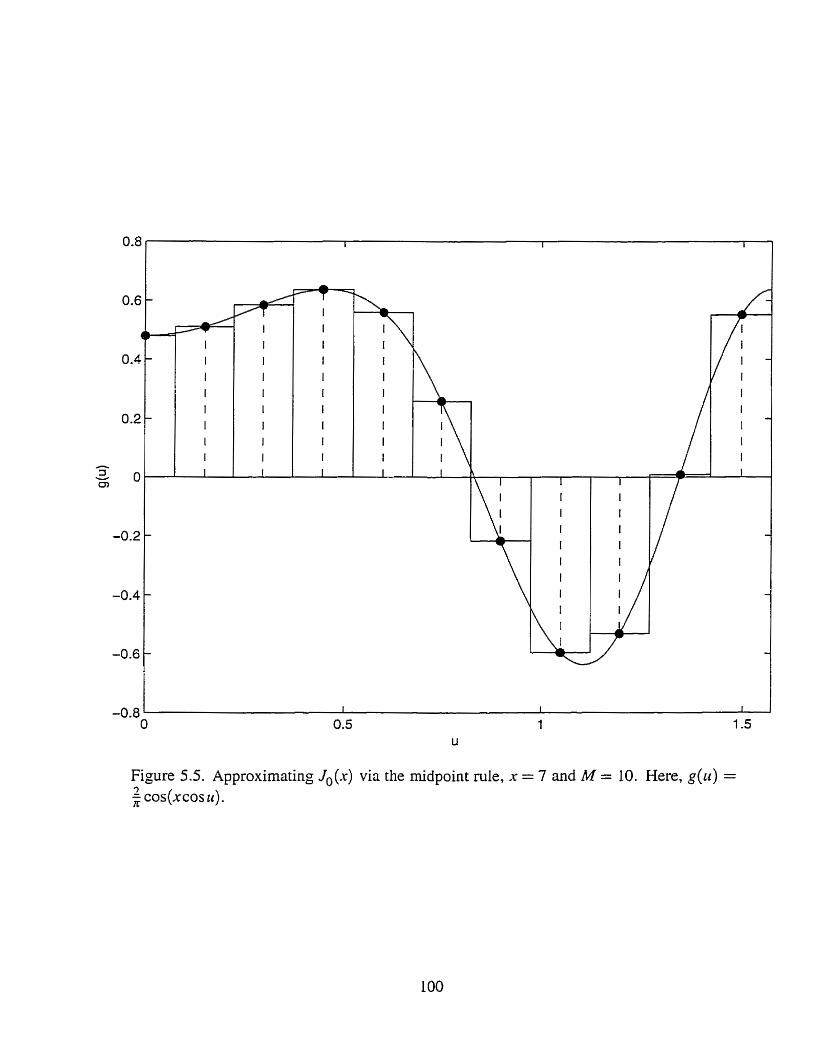
Figure 5.5. Approximating Jo(x) via the midpoint rule, x = 7 and M = 10. Here, g(u) = 1 K COS(XCOS u ) .

a is the left end point of the interval of integration, in Our case a = 0, and

n is the number of panels used in the integration process, in Our case n = M + 1; the

1 cornes about because the panel at origin is half as wide as the other ones. 2

Thus, equation (5.15) specializes to

However, we found the bound of equation (5.16) to be weak, and thus the relationship

between Elel, M, and .r,,, is also weak. An altemate approach is needed.

We observe that al1 quantities in equation (5.14) can be readily computed. We begin by

choosing an error level, and a number of low-frequency oscillators to be included in a sum-

of-sinusoids simulator. Next, we use a search algorithm to determine the smallest value of

xi, for which equation (5.14) holds. We then plot the points (M,.rtnar) for each error level.

Using this procedure, we obtain the family of lines of Figure 5.6. Observe that a small

increase in the number of osciliators can drasticalfy reduce the error in the autocorrelation

function. CVe exploit this a little later, in order to denve a rule-of-thumb relating the number

of low-frequency oscillators M to the breakpoint T,,, in the autocorrelation function.

To illustrate the use of Figure 5.6 consider the following scenario. Suppose we would

like to design a sum-of-sinusoids simulator whose autocorrelation function is within 1 0 ~ ~

of the desired value up to a time lag of 200 S. Also, take wtn = 1 radls. Choosing the line

in Figure 5.6, i.e., the line corresponding to EIeveI = 10-~, we find the point corresponding

to x,,,, = %rmar = 700; on the x-axis we read the corresponding number of low-frequency

oscillators we need. In this case, M = 54. Note that the number of low frequencies needed,

or equivaiently, the number of distinct Doppler shifts, we need is A4 + 1, or 55 here.

In some cases, we are interested in using a srnail number of oscillators. To this end, we

enlarge the lower-left hand corner of Figure 5.6 and present the result in Figure 5.7.

Upon analysis of Figures 5.6 and 5.7, we observe that the breakpoint T , ~ , in the au-

tocorrelation function depends almost linearly on the number of oscillators. Thus, one

Number of oscillators, M-i-1

Figure 5.6. Variation of autocorrelation function breakpoint with the nurnber of low- frequency oscillators (number of distinct Doppler frequency shifts M) and the error level

Elevel

Number of oscillators, M+1

Figure 5.7. Detail of Figure 5.6.

may derive some approximate relationships between the error level, the breakpoint, and

the nurnber of oscillators. To illustrate this process, we choose to quanti@ the relationship

between r,, and M for El,,/ = IO-?. Analysis of Figure 5.7 reveals the slope of the line

corresponding to this error level is approximately 3.5, while the x-axis intercept is roughly

2. This yields 3.5(M + 1) - 1.5

Gnnr = an 1

where the reader is reminded that M + L is the number of distinct Doppler shifts, or equiv-

alently, the number of low-frequency oscillators in the sum-of-sinusoids simulator.

Further malysis of Figures 5.6 and 5.7 reveals that the slopes of the family of lines lie

between 2.5 for small values of the error level and few oscillators, and 4 for large values of

error level and many oscillators. Also, the x-axis intercept seems to lie in the interval [O, 31.

This enables us to obtain the following rule of thumb

We may use equation (5.17) to select an appropriate number of low-frequency oscillators

M given we want the autocorrelation function to be close to the desired value over the in-

terval [O, %,]. Conversely, given a simulator with M low-frequency oscillators, we rnay

use equation (5.17) to determine the value beyond which the autocorrelation deviates sig-

nificantly from the desired value.

It is important to note that the breakpoint rrn, depends on the number of distinct

Doppler frequency shifts M, rather than the nurnber of multipath components N. TO 2-

lustrate this point, we consider

second, N = 18. We still have

two scenarios. In the first, we choose N = 17 and in the

as before. Note that in the first case N = 17, there are nine distinct Doppler frequency shifts.

In the second case N = 18, the number of distinct Doppler frequency shifts has decreased

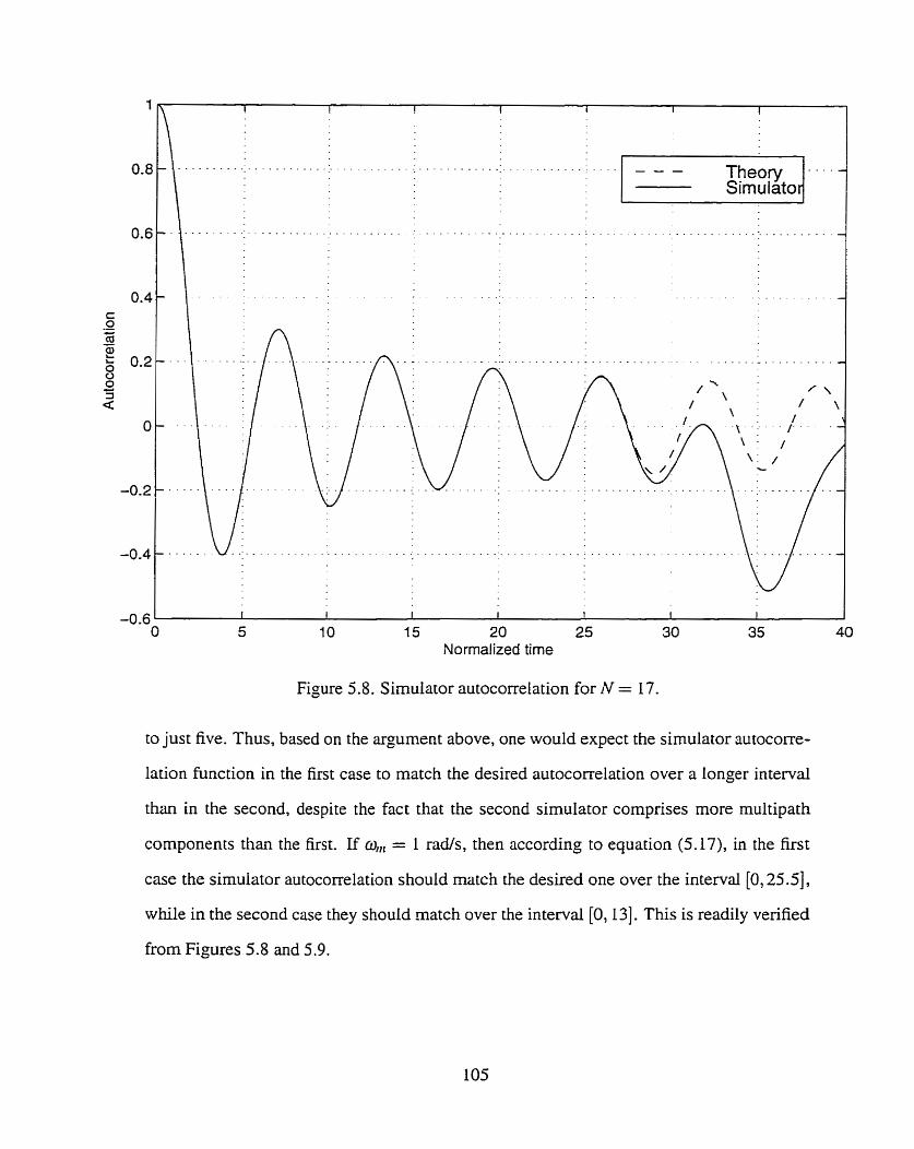
Normalized time

Figure 5.8. Simulator autocorrelation for N = 17.

to just five. Thus, based on the argument above, one would expect the simulator autocorre-

lation function in the first case to match the desired autocorrelation over a longer interval

than in the second, despite the fact that the second simulator comprises more rnultipath

components than the first. If o,, = 1 rads, then according to equation (5.17), in the first

case the simulator autocorrelation should match the desired one over the interval [O, 25.51,

while in the second case they should match over the interval [O, 131. This is readily verified

from Figures 5.8 and 5.9.

Theory . - . -

Sirnulato 1

Normalized time

Figure 5.9. Simulator autocorrelation for N = 18.

Relating the number of low-frequency oscillators to the inaccuracies

In previous sections we have seen that the narrowband Rayleigh flat fading signal can be

characterized by

Note that R( t ) represents an approximation to the fading phenornenon observed in nature.

We need to obtain an estimate on how far this approximation deviates from the desired

value.

Beginning with Jakes [23] many authors have stated that the number of low-frequency

oscillators required to simulate the fading signal is usually srnall. Thus, Jakes [23] suggests

that more than 6 oscillators should suffice for producing a Rayleigh flat fading signal.

Patzold et al. [7], PatzoId et al. [8], and finally Patzold et al. [9] have also suggested

that 7 oscillators is enough to generate a fading signal. In his work, Patzold also uses 10 or

25 oscillators, without an explmation for the increase in number. More recently, Eyceoz

[ 101 has used the Jakes' simulator with 10 oscillators to characterize the fading channel,

Le., to determine the fading coefficients and thus predict the statistics of the fading signai.

However, despite the many suggestions that a srnall number of oscillators is enough

to gnerate a Rayleigh Aat fading signal, some authors use much larger numbers when

trying to fit simulator data to real life measurements. For exarnple, Hoeher [12] uses 500

oscillators to mode1 a wireless channel impulse response. While it is generdly tme that

inclusion of more oscillators leads to a better model, it would be helpful if one knew in

advance how many oscillators would be required to achieve a certain level of accuracy.

In the previous two sections, we have developed quality measures for the performance

of Clarke's model. Thus, we may anaiyze the performance in tems of the envelope pdf, the

envelope cdf, or the autocorrelation function. The phase pdf is the same as the desired pdf

regardless of the number of sinusoids; for this reason, we do not use it as a quality measure.

In the former two cases, we are usually interested in generating a fading signal with pdf

and cdf close to the desired value. Knowledge of the pdf is of interest, for example, in the

determination of the level-crossing rate and the average fade duration.

We may also need to know the value of the autocorrelation function. Behaviour of the

autocorrelation, especially at the origin, is required in the computation of the level-crossing

rate and average fade duration. Furthemore, knowledge of the autocorrelation is useful in

designing sarnpling or divenity schemes; Le., usehl in obtaining independent samples,

or placing antennas at points which experience independent fading. It has been known, as

early as Jakes [23], that the autocorrelation function of the simulator signal breaks down for

large enough time lags. In the previous section we have determined a relationship between

the number of oscillators and the interval over which the autocorrelation function is close

to the desired value.

To use the results of this thesis successful~y, the engineer would first have to decide

which statistic is most important to hisher work. Then, using an appropriate quaiity mea-

sure, as illustrated in this chapter, the engineer may determine the number of osciilators

required by the simulator. If, however, there is more than one statistic relevant to the

project, the engineer may determine the number of oscillators required for each statistic,

and simply pick the largest value for the practical implementation.

Chapter 6

Conclusion

One method of simulating the multipath fading encountered on Rayleigh Bat fading nar-

rowband wireless channels is based upon the sum-of-sinusoids model. Such simulators are

readily derived from consideration of the physical phenornenon. The work of Clarke [3]

sumar izes the important characteristics of such simulators, and sets the stage for further

developments, such as those of Jakes [23]. Clarke's rnodel and Jakes' fading channel sim-

ulator, as well as other work in the area of sum-of-sinusoids simulators were presented in

Chapter 2. In addition, we presented Patzold's results relating to the statistical properties

of Jakes' sirnulator.

In Chapter 3, we derived the statisticd properties of sum-of-sinusoids simulators in

generd. The starting point of the analysis is the assumptions made by Clarke in derivinp

a mathematical model of multipath Rayleigh fading. We noted that this is different from

the starting point in Patzold's andysis; his analysis is based on the assumption that the

quadrature components of the fading signal are approximately Gaussianly distributed and

uncorrelated, and hence independent.

The results denved for the envelope and phase pdf's are applied to determine the statis-

tics of Clarke's model and Jakes' fading channel sirnulator. We also cornpute the autocor-

relation functions for the signals of the two models. The main reason for doing this is to

determine whether the assumptions made by Jakes in simpliwing Clarke's model are jus-

tified. We show that they are not. The signal produced by Clarke's model is shown to be

wide-sense stationary, while that produced by Jakes' simulator is shown to not be wide-

sense stationary. The chapter concludes with a discussion of ergodicity and how it applies

to surn-of-sinusoids models and simulators.

It is generally desired to have an efficient method for generating fading signais. Viewed

in this light, Jakes' approach presents an interesting point. That is, if we are able to reduce

the complexity of the model, i.e., the number of low-frequency oscillators, then the gener-

ation of the signal is more efficient. In Chapter 4, we attempt to improve the performance

of Jakes' simulator through simple modifications. We found that introduction of random

phase shifts in the low-frequency oscillators removes the stationarity problems; that is, the

resulting signal is wide-sense stationary. However, the intuitive relationship between the

physicd parameters and the simulator structure is lost. Also, the phase shifts of the corn-

ponents of the resuiting multipath fading signal are still dependent. This may have adverse

effects on the determination of higher order statistics through simulation. We conclude the

chap ter with a note regarding the possibility of reducing the complexity of Clarke's model.

We found that the least number of low-frequency oscillators required is equal to the nurnber

of distinct Doppler frequency shifts, counting positive and negative shifts as one. However,

we must be careful in determinhg the gain of each branch for each Iow-frequency oscilla-

tor, i.e., we must include al1 phase shifts corresponding to a particular Doppler frequency

shift.

Another point of interest is how accurate the statistics of the fading signal produced

by the sum-of-sinusoids simulator are. In Chapter 5, we showed how the results obtained

in Chapter 3 can be used to derive quality measures. Depending on the accuracy required

of the simulator, the appropriate number of low-frequency oscillaton, or equivalently, si-

nusoids, to be included in the simulator can be determined. The quality measures rnay be

derived with respect to either the envelope pdf or cdf, or the autocorrelation function. We

do not use the phase pdf as the basis of quality measures. The phase pdf is equal to the

desired pdf, regardless of the number of low-frequency oscillators, and thus conveys little

information about the performance of the simulator.

To denve the quaiity measures, we may use criteria such as the maximum error, mean

square error, variance, or an approach sirnilar to that of Young [22]. In the event that we

wish to control the accuracy of the envelope pdf, cdf, and the signai autocorrelation, we pro-

ceed as indicated for each function. Then, for the practical implementation, we select the

largest number of sinusoids obtained through each of the quality measures. We conclude

by noting that the interval over which the autocorrelation function closely approximates

the desired autocorrelation function is directly related to the number of Doppler frequency

shifts. Prior to this, we noted that the wide-sense stationarity character of the fading signal

was dependent upon inclusion of al1 phase shifts, i.e., combining the phase shifts as an ap-

propriate gain for waves experiencing the same Doppler shift. Failure to do so, as in Jakes'

case, leads to non-stationarity problems.

Dunng the writing of this thesis, the various methods employed and the results denved

have sugpested other areas which might be of interest to future researchen. For exarnple,

approaches sirnilar to those used in this thesis may be used to denve other results of in-

terest to the wireless engineer. In particular, the random walk in the plane may be used

to derive analytical results to problems such as determination of level-crossing rates, fade

duration distribution, or the variance of the average fade duration. Another area of interest

is design of fading channel simulaton with arbitrary arriva1 angles pdf. Still another area of

possible interest is design of three-dimensional fading channel simulators based on sum-of-

sinusoids. Such scenarios have been shown to provide better fading channel models in the

case of heavily urbanized areas [6 ] . Future work in this area would potentially culminate

with the development of a three-dimensional fading channel simulator.

References

jing Due to Builc [ I ] J. F. Ossanna, Jr., "A Model for Mobile Radio Fa( jing Reflections:

Theoretical and Experimental Fading Waveform Power S pectra", Bell Syst. Tech. J, pp. 2935-297 1, NOV. 1964.

[2] E. N. Gilbert, "Energy Reception for Mobile Radio", Bell Syst. Tech. J., pp. 1779-

1803, Oct. 1965.

[3] R. H. Clarke, "A Statistical Theory of Mobile-Radio Reception", Bell Syst. Tech. J.,

pp. 957- 1000, Ju1.-Aug. 1968.

[4] M. J. Gans, "A Power-spectral Theory of Propagation in the Mobile Radio Environ-

ment", IEEE ?i-ans. Nh. Tech., vol. VT-2 1, February 1972, pp. 27-38.

[5] P. Dent, G. E. Bottomley, and T. Croft, "lakes' Fading Model Revisited", Electron.

Lett., vol. 29. no. 3, pp. 1 162- 1 163, Jun. 1993.

[6] T. Aulin, "A Modified Model for the Fading Signal at a Mobile Radio Channel", IEEE

Trans. Veh. Tech., vol. VT-28, no. 3, pp. 182-203, Aug. 1979.

[7] M. Patzold, U. Killat, and F. Laue, "A Deterministic Digital Simulation Model for

Suzuki Processes with Application to a Shadowed Rayleigh Land Mobile Radio

Channel", i E E Tram. Veh. Tech., vol. 45, no. 2, pp. 318-33 1, May 1996.

[SI M. Patzold, U. Killat, F. Laue, and Y. Li, "On the Statisticd Properties of Determinis-

tic Simulation Models for Mobile Fading Charnels", IEEE Trans. Veh. Tech., vol. 47,

no. 1, pp. 254-269, Feb. 1998.

[9] M. Patzold and E Laue, "Statistical properties of Jakes' fading channel sirnulator",

VTC '98 Conference Record, vol. II, pp. 712-718, Ottawa, Ontario, Canada, May

1998.

1101 T. Eyceoz, A. Duel-Hallen, and H. Hallen, "Deterministic Channel Modeling and

Long Range Prediction of Fast Fading Mobile Radio Channels", IEEE Commun. Lett.,

vol. 2, no. 9, pp. 254-256, Sep. 1998.

[ I l ] P. A. Bello, "Characterization of Randornly Time-Variant Linear Channels", IEEE

Trarrs. Cornrnrrn. Syst., vol. CS- 1 1, pp. 360-393, Dec. 1963.

[12] P. Hoeher, "A Statistical Discrete-Time Mode1 for the WSSUS Multipath Channel",

IEEE Trnns. Veh. Tech., vol. 41, no. 4, pp. 46 1468, Nov. 1992.

Cl31 G. A. Anedondo and J. 1. Smith, "Voice and Data Transmission in a Mobile Radio

Channel at 850 MHz", IEEE Tram. Veh. Tech., vol. VT-26, no. 1, pp. 88-93, Feb.

1977

[14] S. O. Rice, "Mathematical Andysis of Random Noise", Bell Syst. Tech. J., vol. 23,

pp. 282-332, Jul. 1944.

[15] S. O. Rice, "Mathematical Analysis of Random Noise", Bell Syst. Tech. J., vol. 24,

pp. 46-156, Jan. 1945.

[16] S. O. Rice, "Distribution of the Extreme Values of the Sum of n Sine Waves Phased

at Randorn", Quart. Appl. Math., vol. XII, no. 4, pp. 375-381, Jan. 1955.

[17] 1. Goldman, "Statistical Properties of a Sum of Sinusoids and Gaussian Noise and its

Generalization to Higher Dimensions", Bell Syst. Tech. J., vol. 53, no. 4, pp. 557-580,

Apr. 1974.

[183 S. O. Rice, "Probability Distributions for Noise Plus Several Sine Waves - The Prob-

lem of Computation", IEEE Trnns. Commun., voi. COM-22, pp. 851-853, Jun. 1974.

[19] C. W. Helsîxom, "Computing the Distribution of Sums of Random Sine Waves and

of Rayleigh-Distnbuted Randorn Variables by Saddle-Point Integration", IEEE Tram.

Commltn., vol. 45, no. 1 1, pp. l487- 1494, Nov. 1997.

[20] M. Slack, "The Probability Distribution of Sinusoidal Oscillations Combined in Rm-

dom Phase", Proc. IEE, vol. 93, pt. C, no. 22, pp. 76-86, Mar. 1946.

[2 11 W. R. Bennett, "Distribution of the Sum of Randody Phased Components", Qrtart.

Appl. Math.", vol. 5, pp. 385-393, Jan. 1948.

[22] D. I. Young, "The Generation of Correlated Rayleigh Random VXiates By Discrete

Fourier Transform and Quality Measures for Random Variate Generation", M. Sc.

Thesis, Queen's University, Kingston, Canada, 1997.

[23] W. C. Jakes, Microivnvr Mobile Conzrnrtnications, IEEE edition, IEEE Press, New

York, 1994.

[24] G. L. Stüber, Prirzciples of Mobile Comrnrtnicatiorz, Kluwer Academic Publishers,

Boston, 1996.

[25] T. S. Rappapon, WireZess Commcmications: Principles and Prnctice, Prentice Hall

PTR, Upper Saddle River, New Jersey, 1996.

[26] G. N. Watson, A Trearise on the Theory of Bessel Fimcrioïu, Cambridge Mathematical

Library edition, Cambridge University Press, New York, 1995.

[27] S. Bochner, Lectures on Fourier Integrals, Annals of Mathematics Studies, Snidy 42,

Princeton University Press, Princeton, New Jersey, 1959.

1281 R. E. Ziemer and W. H. Tranter, Principles of Communicntions: Systems, Modulation,

and Noise, 4th ed., John Wiley & Sons, Inc., New York, 1995.

[29] A. Papoulis, Probability, Random Variables, and Stochastic Processes, 3rd ed.,

McGraw-Hill, hc., Toronto, 199 1.

[30] J. G. Proakis, Digital Contrtrrnications, 3rd ed., McGraw-Hill, Inc., New York, 1995.

[3 11 W. A. Gardner, Introduction to Random Processes: With Applications to Signals and

Systems, Macmillan Publishing Company, New York, 1985.

[32] J. L. Doob Stochnstic Processes, 3rd printing, John Wiley & Sons, Inc., New York,

1960.

[33] R. M. Gray and L. D. Davisson, Random Processes: A Mathematical Approach for

Engineers, Prentice-Hall, Inc., Englewood Cliffs, New Jersey, 1986.

[34] J. Stewart, Calc~ilrts: Early Trnnscedentnls, 2nd ed., BrooksICole Publishing Com-

pany, Pacific Grove, CA, 199 1.

[35] R. Bracewell, The Fourier Transforni and Its Application, McGraw-Hill Book Com-

pany, New York, 1965.

[36] 1. S. Gradshteyn and 1. M. Ryzhik; Alian Jeffrey, editor, Table of integrals. series, and

prodttcts, 5th edition, Acadernic Press, Inc., New York, 1994.

[37] M. Abramowitz and 1. A. Stegun, Handbook of Mathematical F~mctions rvith For-

mulas. Graphs, and Mathematical Tables, 10th printing, U. S. Govemment Printing

Office, Washington, D. C., 1972.

[38] F. Oberhettinger, Fourier Transfoms of Distribrltions and nzeir I~zverses: A Collec-

tion of Tables, Academic Press, New York, 1973.