A Submillimeter Imaging Surveyof Ultracompact HII RegionsThesis byTodd R. HunterIn Partial Ful�llment of the Requirementsfor the Degree ofDoctor of Philosophy

1 8 9 1

CA

LIF

OR

NIA

I

NS T IT U T E O F T

EC

HN

OL

OG

YCalifornia Institute of TechnologyPasadena, California1997(Submitted September 17, 1996)

ii

c 1997Todd R. HunterAll Rights Reserved

iii

Comet Hyakutakephotographed on 25 March 1996at Joshua Tree National Park, California

ivAcknowledgementsMuch of the success of this thesis can be traced to Larry Ramsey and Je� Hallfor introducing me to instrumentation work at Penn State. My experience as aVLA summer student in 1990 also in�uenced me immeasurably by bringing radioastronomy to life in the Land of Enchantment, where I made some lifelong friends.Looking back, I am pleased that Craig Walker convinced me to apply to Caltech. Ithank my graduate advisor Tom Phillips for teaching me how to tune SIS receivers atCSO and welcoming me into the submillimeter group, a unique collection of peoplethat always manages to �nish �rst when it counts. Thanks to Pat Scha�er and JacobKooi for the world's best receivers (and all those lab tools of theirs that I didn't steal).Special thanks go to Harvey Moseley's family and colleagues at NASA/Goddard forall their help and hospitality. For answering my frequent computer and scienti�cquestions, Darek Lis deserves special mention. Similar recognition goes to GeneSerabyn for help with optics and for constructive comments on this manuscript, and toNing Wang whose determination led to the timely commissioning of SHARC. Thanksalso to Maryvonne Gerin and Peter Schilke for showing me all the neat features ofGRAPHIC. For keeping the telescope running, thanks to the CSO sta�, especiallyTaco, a dependable source of advice and humorous stories. To Greg Taylor, thanksfor your lessons on VLA data and introducing me to the members of the Arcetrigroup. Thanks to Natalie Merchant and the 10kM for audio encouragement duringlong summer days of programming SHARC at the summit of Mauna Kea, where bythe force of will my lungs were �lled. Thanks to Eric Howard for his near-infrareddata on S255, Chris DePree for his radio data on K3-50, and Debra Shepherd andPeter Hofner for sharing their millimeter and radio data on G45 and G75. Much ofthe research reported here was augmented by the patient advice and frequent noggin-usage of Dominic Benford and Robert Knop. Finally, with all the encouragement andhelp from my family back East, these past �ve years have been well worth the e�ort.

vAbstractThis research explores the process of massive star formation in the Galaxy throughsubmillimeter continuum and spectral line observations of ultracompact HII (UCHII)regions. First, I describe the design and operation of the Submillimeter High AngularResolution Camera (SHARC)�a 24-pixel bolometer array camera for broadband con-tinuum imaging at 350 and 450�m at the Caltech Submillimeter Observatory (CSO).Detailed information is included on the re�ective o�-axis optical design and the in-strument control software interface. Second, I present 1000 to 1200 resolution SHARCimages of 350 and 450�m continuum emission from a sample of 17 UCHII regionswith di�erent radio morphologies. Although the dust emission typically peaks at ornear the UCHII region, additional sources are often present, sometimes coincidentwith the position of H2O masers. The combination of submillimeter, millimeter andIRAS far-infrared �ux densities forms the basis of greybody models of the spectralenergy distributions. The average dust temperature is 40 � 10 K and the averagegrain emissivity index (�) is 2:00 � 0:25. Using a radiative transfer program thatsolves for the dust temperature versus radius, the distribution of dust around UCHIIregions is modeled with a power-law spherical density pro�le to match the observedradial �ux density pro�les. By �xing the source boundary at the outer limit of thesubmillimeter emission, the resulting density pro�les n(r) / r�p can be classi�edinto four categories: 3 regions exhibit p = 2 (isothermal sphere), 4 exhibit p = 1:5(dynamical collapse), 2 exhibit p = 2 in the outer regions and p = 1:5 in the innerregions, and 6 exhibit p = 1 (logatropic). Although these simpli�ed models maynot be unique, a good correlation between the dust luminosity-to-mass ratio and thetemperature indicates that the more centrally-condensed sources exhibit higher starformation rates. Third, I present 2000 to 3000 resolution CO maps which reveal bipolarout�ows from 15 out of 17 UCHII regions. The out�ow mechanical luminosities andmass ejection rates follow the scaling relations with bolometric luminosity established

vifor less luminous pre-main sequence stars. However, in contrast to lower luminositysources, the momentum from stellar radiation pressure is comparable to that requiredto drive the out�ows. Many regions show evidence of separate, overlapping out�ows.In a �nal detailed study, 200 resolution images obtained with the Owens Valley Mil-limeter Array reveal multiple out�ows emanating from the molecular core containingthe UCHII region G45.12+0.13, while simultaneous out�ow and infall motion is seentoward the neighboring, less-evolved core containing G45.07+0.13.

viiContentsAcknowledgements ivAbstract v1 Introduction and Background 11.1 Massive star formation : : : : : : : : : : : : : : : : : : : : : : : : : : 11.2 Thesis outline : : : : : : : : : : : : : : : : : : : : : : : : : : : : : : : 102 The Submillimeter High Angular Resolution Camera (SHARC) 122.1 Instrument overview : : : : : : : : : : : : : : : : : : : : : : : : : : : 132.2 Optical design : : : : : : : : : : : : : : : : : : : : : : : : : : : : : : : 212.3 Optical performance : : : : : : : : : : : : : : : : : : : : : : : : : : : 372.4 Instrument control system : : : : : : : : : : : : : : : : : : : : : : : : 422.5 Data reduction : : : : : : : : : : : : : : : : : : : : : : : : : : : : : : 482.6 Sensitivity : : : : : : : : : : : : : : : : : : : : : : : : : : : : : : : : : 533 Submillimeter Continuum Images of UCHII Regions 563.1 The characteristics of interstellar dust : : : : : : : : : : : : : : : : : : 563.2 Computation of dust column density and mass from submillimeter �uxdensity : : : : : : : : : : : : : : : : : : : : : : : : : : : : : : : : : : : 613.3 HIRES IRAS images : : : : : : : : : : : : : : : : : : : : : : : : : : : 653.4 Calibration and pointing accuracy of the SHARC images : : : : : : : 843.5 SHARC images of cometary UCHII regions : : : : : : : : : : : : : : : 873.6 SHARC images of shell-like UCHII regions : : : : : : : : : : : : : : : 1063.7 SHARC images of unresolved UCHII regions : : : : : : : : : : : : : : 1153.8 SHARC image of the G75 Complex (ON 2) : : : : : : : : : : : : : : : 1253.9 Greybody models : : : : : : : : : : : : : : : : : : : : : : : : : : : : : 129

viii3.10 Density pro�les : : : : : : : : : : : : : : : : : : : : : : : : : : : : : : 1443.11 Luminosity to mass ratios : : : : : : : : : : : : : : : : : : : : : : : : 1713.12 Summary : : : : : : : : : : : : : : : : : : : : : : : : : : : : : : : : : 1734 Molecular Out�ows from UCHII Regions 1764.1 Characteristics of molecular out�ows : : : : : : : : : : : : : : : : : : 1764.2 Possible mechanisms of jet-driven out�ows : : : : : : : : : : : : : : : 1824.3 Out�ows from high-mass star-forming regions : : : : : : : : : : : : : 1864.4 CO spectra : : : : : : : : : : : : : : : : : : : : : : : : : : : : : : : : 1874.5 CO out�ow maps : : : : : : : : : : : : : : : : : : : : : : : : : : : : : 1904.6 Calculation of out�ow energetics : : : : : : : : : : : : : : : : : : : : : 2064.7 Scaling relations : : : : : : : : : : : : : : : : : : : : : : : : : : : : : : 2114.8 Summary : : : : : : : : : : : : : : : : : : : : : : : : : : : : : : : : : 2175 Active Star Formation toward the G45.12+0.13 and G45.07+0.13UCHII Regions 2195.1 Introduction : : : : : : : : : : : : : : : : : : : : : : : : : : : : : : : : 2205.2 Observations : : : : : : : : : : : : : : : : : : : : : : : : : : : : : : : : 2245.3 Molecular out�ows : : : : : : : : : : : : : : : : : : : : : : : : : : : : 2265.4 Continuum emission : : : : : : : : : : : : : : : : : : : : : : : : : : : 2425.5 Discussion : : : : : : : : : : : : : : : : : : : : : : : : : : : : : : : : : 2455.6 Conclusions : : : : : : : : : : : : : : : : : : : : : : : : : : : : : : : : 2486 Summary 250References 252Appendix A: SHARC Cryostat Manual 277Appendix B: SHARC Software Manual 286Appendix C: Input parameters for the OUTFLOW program 294

ixList of Figures2.1 Photograph of the bolometer array detector : : : : : : : : : : : : : : 192.2 Layout of the ellipsoid re-imager : : : : : : : : : : : : : : : : : : : : : 262.3 Strehl ratios versus chopper angle : : : : : : : : : : : : : : : : : : : : 282.4 Spot diagrams across the SHARC focal plane : : : : : : : : : : : : : 302.5 Sketch of the internal cryostat optics : : : : : : : : : : : : : : : : : : 322.6 SHARC �lter arrangement : : : : : : : : : : : : : : : : : : : : : : : : 342.7 Strehl ratio versus dewar rotation angle : : : : : : : : : : : : : : : : : 382.8 CSO/SHARC beam map at 350�m : : : : : : : : : : : : : : : : : : : 392.9 SHARC �lter transmission curves : : : : : : : : : : : : : : : : : : : : 412.10 SHARC Server computer display : : : : : : : : : : : : : : : : : : : : 442.11 OTF map computer display : : : : : : : : : : : : : : : : : : : : : : : 472.12 SHARC NEFDs achieved at 350 and 450�m : : : : : : : : : : : : : 542.13 SHARC sensitivity vs. integration time at 450�m : : : : : : : : : : : 553.1 Mean �ux density-weighted grain radius for the n(a) / a�3:5 distribution 623.2 HIRES IRAS maps of G19.61-0.23 : : : : : : : : : : : : : : : : : : : : 713.3 HIRES IRAS maps of G29.96-0.02 : : : : : : : : : : : : : : : : : : : : 723.4 HIRES IRAS maps of G34.26+0.14 : : : : : : : : : : : : : : : : : : : 733.5 HIRES IRAS maps of G45.1+0.1 : : : : : : : : : : : : : : : : : : : : 743.6 HIRES IRAS maps of the K3-50 complex : : : : : : : : : : : : : : : : 753.7 HIRES IRAS maps of G75.8+0.4 : : : : : : : : : : : : : : : : : : : : 763.8 HIRES IRAS maps of W3(OH) : : : : : : : : : : : : : : : : : : : : : 773.9 HIRES IRAS maps of G138.30+1.56 : : : : : : : : : : : : : : : : : : 783.10 HIRES IRAS maps of G139.909+0.197 : : : : : : : : : : : : : : : : : 793.11 HIRES IRAS maps of Monoceros R2 : : : : : : : : : : : : : : : : : : 803.12 HIRES IRAS maps of GGD12-15 : : : : : : : : : : : : : : : : : : : : 81

x3.13 HIRES IRAS maps of the S255 complex : : : : : : : : : : : : : : : : 823.14 HIRES IRAS maps of G240.31+0.07 : : : : : : : : : : : : : : : : : : 833.15 2.0 cm radio continuum image of G34.3+0.2 : : : : : : : : : : : : : : 883.16 2.0 cm radio continuum image of G34.26+0.14 : : : : : : : : : : : : : 893.17 350 and 450�m images of G34.3+0.15 : : : : : : : : : : : : : : : : : : 903.18 H2CO 31;2 � 21;1 map around G34.3+0.2SE : : : : : : : : : : : : : : : 923.19 H2CO 31;2 � 21;1 spectrum of G34.3+0.2SE : : : : : : : : : : : : : : : 933.20 2.0 cm radio continuum image of G29.96-0.02 : : : : : : : : : : : : : 943.21 800�m image of G29.96-0.02 : : : : : : : : : : : : : : : : : : : : : : : 953.22 450�m image of G29.96-0.02 : : : : : : : : : : : : : : : : : : : : : : : 963.23 6 cm radio continuum image of G19.61-0.23 : : : : : : : : : : : : : : 973.24 800�m image of G19.61-0.23 : : : : : : : : : : : : : : : : : : : : : : : 983.25 450�m image of G19.61-0.23 : : : : : : : : : : : : : : : : : : : : : : : 993.26 3.6 cm VLA image of GGD12-15 : : : : : : : : : : : : : : : : : : : : 1003.27 350�m image of the GGD12-15 : : : : : : : : : : : : : : : : : : : : : 1013.28 6 cm radio continuum image of Mon R2 : : : : : : : : : : : : : : : : 1033.29 350�m image of the Mon R2 complex : : : : : : : : : : : : : : : : : : 1043.30 VLA 3.6 cm image of the K3-50 complex : : : : : : : : : : : : : : : : 1073.31 800�m image of the K3-50 complex : : : : : : : : : : : : : : : : : : : 1093.32 SHARC 350�m image of the K3-50 complex : : : : : : : : : : : : : : 1103.33 18 cm radio continuum image of W3(OH) : : : : : : : : : : : : : : : 1113.34 800�m image of W3(OH) : : : : : : : : : : : : : : : : : : : : : : : : : 1133.35 350�m image of W3(OH) : : : : : : : : : : : : : : : : : : : : : : : : : 1143.36 350�m image of G240.31+0.07 : : : : : : : : : : : : : : : : : : : : : : 1153.37 350�m image of G138.295+1.555 : : : : : : : : : : : : : : : : : : : : 1173.38 350�m image of the G139.909+0.197 complex : : : : : : : : : : : : : 1193.39 350�m image of the S255 complex : : : : : : : : : : : : : : : : : : : : 1203.40 350�m image of the S255 complex : : : : : : : : : : : : : : : : : : : : 1223.41 CS J=7!6 image of the S255 complex : : : : : : : : : : : : : : : : : 1233.42 K-band & 350�m image of S255-FIR2 : : : : : : : : : : : : : : : : : 124

xi3.43 800�m image of G75.84+0.34 : : : : : : : : : : : : : : : : : : : : : : 1253.44 6 cm radio continuum image of G75.78+0.34 : : : : : : : : : : : : : : 1263.45 800�m image of the G75 complex : : : : : : : : : : : : : : : : : : : : 1273.46 450�m image of the G75 complex : : : : : : : : : : : : : : : : : : : : 1283.47 Histograms of the UCHII greybody models : : : : : : : : : : : : : : : 1333.48 Spectral energy distribution of G19.61-0.23 : : : : : : : : : : : : : : : 1353.49 Spectral energy distribution of W3(OH) : : : : : : : : : : : : : : : : 1363.50 Spectral energy distribution of G29.96-0.02 : : : : : : : : : : : : : : : 1363.51 Spectral energy distribution of G34.3+0.2 : : : : : : : : : : : : : : : 1373.52 Spectral energy distribution of K3-50A : : : : : : : : : : : : : : : : : 1373.53 Spectral energy distribution of K3-50C : : : : : : : : : : : : : : : : : 1383.54 Spectral energy distribution of Monoceros R2 : : : : : : : : : : : : : 1383.55 Spectral energy distribution of GGD12-15 : : : : : : : : : : : : : : : 1393.56 Spectral energy distribution of G192.584-0.041 : : : : : : : : : : : : : 1393.57 Spectral energy distribution of S255-FIR2 : : : : : : : : : : : : : : : 1403.58 Spectral energy distribution of G45.07+0.13 : : : : : : : : : : : : : : 1403.59 Spectral energy distribution of G45.12+0.13 : : : : : : : : : : : : : : 1413.60 Spectral energy distribution of G75.78+0.34 : : : : : : : : : : : : : : 1413.61 Spectral energy distribution of G75.84+0.40 : : : : : : : : : : : : : : 1423.62 Spectral energy distribution of G139.909+0.197 : : : : : : : : : : : : 1423.63 Spectral energy distribution of G138.295+1.555 : : : : : : : : : : : : 1433.64 Spectral energy distribution of G240.31+0.01 : : : : : : : : : : : : : : 1433.65 Flux pro�le of Uranus as the instrument response pattern : : : : : : : 1513.66 350�m image of Uranus in celestial coordinates : : : : : : : : : : : : 1523.67 Flux pro�le of G240.31+0.07 : : : : : : : : : : : : : : : : : : : : : : : 1533.68 Flux pro�le of G19.61-0.23 : : : : : : : : : : : : : : : : : : : : : : : : 1543.69 Flux pro�le of G29.96-0.02 : : : : : : : : : : : : : : : : : : : : : : : : 1553.70 Flux pro�le of W3(OH) : : : : : : : : : : : : : : : : : : : : : : : : : : 1563.71 Flux pro�le of K3-50A : : : : : : : : : : : : : : : : : : : : : : : : : : 1573.72 Flux pro�le of S255 FIR2 : : : : : : : : : : : : : : : : : : : : : : : : : 158

xii3.73 Flux pro�le of G75.78+0.34 : : : : : : : : : : : : : : : : : : : : : : : 1593.74 Flux pro�le of G45.07+0.13 : : : : : : : : : : : : : : : : : : : : : : : 1603.75 Flux pro�le of G34.3+0.2 : : : : : : : : : : : : : : : : : : : : : : : : : 1613.76 Flux pro�le of K3-50C : : : : : : : : : : : : : : : : : : : : : : : : : : 1623.77 Flux pro�le of G45.12+0.13 : : : : : : : : : : : : : : : : : : : : : : : 1633.78 Flux pro�le of GGD12-15 : : : : : : : : : : : : : : : : : : : : : : : : 1643.79 Flux pro�le of G192.584-0.041 : : : : : : : : : : : : : : : : : : : : : : 1653.80 Flux pro�le of G138.295+1.555 : : : : : : : : : : : : : : : : : : : : : 1663.81 Flux pro�le of G139.909-0.197 : : : : : : : : : : : : : : : : : : : : : : 1673.82 Predicted spectral energy distributions : : : : : : : : : : : : : : : : : 1693.83 Predicted temperature distributions : : : : : : : : : : : : : : : : : : : 1703.84 Dust core luminosity and LFIR=Mdust ratio vs. temperature : : : : : : 1724.1 CO out�ow spectra : : : : : : : : : : : : : : : : : : : : : : : : : : : : 1894.2 CO J=2!1 map of K3-50 : : : : : : : : : : : : : : : : : : : : : : : : 1914.3 CO J=3!2 map of K3-50A : : : : : : : : : : : : : : : : : : : : : : : 1924.4 CO J=3!2 map of W3(OH) : : : : : : : : : : : : : : : : : : : : : : 1934.5 CO J=3!2 map of G138.295+1.555 : : : : : : : : : : : : : : : : : : 1944.6 CO J=3!2 map of G139.909+0.197 : : : : : : : : : : : : : : : : : : 1954.7 CO J=3!2 map of G240.31+0.07 : : : : : : : : : : : : : : : : : : : : 1964.8 CO J=2!1 map of the G75.8+0.3 complex : : : : : : : : : : : : : : 1974.9 CO J=2!1 map of G75.84+0.40 : : : : : : : : : : : : : : : : : : : : 1984.10 CO J=3!2 map of the S255 complex : : : : : : : : : : : : : : : : : : 1994.11 CO J=2!1 map of G19.61-0.23 : : : : : : : : : : : : : : : : : : : : : 2004.12 CO J=2!1 map of G29.96-0.02 : : : : : : : : : : : : : : : : : : : : : 2014.13 CO J=3!2 map of G5.97-1.18 : : : : : : : : : : : : : : : : : : : : : 2024.14 CO J=3!2 map of the Cepheus-A complex : : : : : : : : : : : : : : 2044.15 CO J=3!2 map including G45.45+0.06 & G45.47+0.05 : : : : : : : 2054.16 Out�ow mechanical luminosity vs. bolometric luminosity : : : : : : : 2124.17 Out�ow force vs. bolometric luminosity : : : : : : : : : : : : : : : : : 214

xiii4.18 Mass out�ow rate vs. bolometric luminosity : : : : : : : : : : : : : : 2165.1 CO J=3!2 map of G45.12+0.13 & G45.07+0.13 : : : : : : : : : : : 2225.2 CO spectra of G45.12+0.13 and G45.07+0.13 : : : : : : : : : : : : : 2275.3 CS 7!6 spectrum of G45.12+0.13 and G45.07+0.13 : : : : : : : : : : 2285.4 CO J=2!1 maps of G45.12+0.13 : : : : : : : : : : : : : : : : : : : : 2295.5 CO J=6!5 map of G45.12+0.13 : : : : : : : : : : : : : : : : : : : : 2305.6 CO J=6!5 map of G45.07+0.13 : : : : : : : : : : : : : : : : : : : : 2315.7 C18O J=1!0 map of G45.12+0.13 : : : : : : : : : : : : : : : : : : : 2355.8 Channel maps of 13CO J=1!0 toward G45.12+0.13 : : : : : : : : : 2375.9 CO J=3!2 map of G45.12+0.13 : : : : : : : : : : : : : : : : : : : : 2385.10 CS J=7!6 map of G45.12+0.13 : : : : : : : : : : : : : : : : : : : : 2395.11 CS J=2!1 spectrum of G45.07+0.13 : : : : : : : : : : : : : : : : : : 2405.12 CS J=2!1 channel maps of G45.07+0.13 : : : : : : : : : : : : : : : 2415.13 800, 450 and 350�m continuum maps of the G45 complex : : : : : : : 2425.14 110 GHz continuum map of G45.12+0.13 : : : : : : : : : : : : : : : : 2445.15 98 GHz continuum map of G45.07+0.13 : : : : : : : : : : : : : : : : 246

xivList of Tables3.1 UCHII regions analyzed with HIRES processing : : : : : : : : : : : : 663.2 Observed properties of the dust clumps toward G34.3+0.2 : : : : : : 913.3 Observed properties of the dust clumps in Mon R2 : : : : : : : : : : 1053.4 Greybody model parameters of dust around UCHII regions : : : : : : 1323.5 Comparison of the one- and two-component greybody models : : : : 1343.6 Summary of dust density pro�les : : : : : : : : : : : : : : : : : : : : 1744.1 Observed and computed parameters of bipolar out�ows : : : : : : : : 2105.1 Summary of CSO spectroscopic observations of G45 : : : : : : : : : 2245.2 Summary of OVRO observations of G45 : : : : : : : : : : : : : : : : 2265.3 Observed properties of the CS J=7!6 transition : : : : : : : : : : : 2285.4 Properties of the G45.12+0.13 molecular out�ow : : : : : : : : : : : 2325.5 Properties of the G45.07+0.13 molecular out�ow : : : : : : : : : : : 2345.6 Out�ow masses derived from the 13CO J=1!0 maps : : : : : : : : : 2365.7 Millimeter and submillimeter continuum �uxes of G45 : : : : : : : : 2435.8 Greybody model parameters of G45.12+0.13 and G45.07+0.13 : : : 243

1Chapter 1 Introduction and Background1.1 Massive star formationMassive stars exert a dominant force on the interstellar medium throughout theirlives. Powerful out�ows, stellar winds, HII regions and supernova explosions combineto shape the appearance of galaxies, most notably the starbursts. With this factin mind, the understanding of massive star formation in our Galaxy becomes anessential goal with universal application in astrophysics. Traditionally, this goal hasbeen di�cult to achieve due to the extreme optical extinction by interstellar dust inactive star formation regions. In recent decades, the discovery of ultracompact HII(UCHII) regions at radio wavelengths has provided a promising target in this research.Observations indicate a link between UCHII regions, H2O masers, dust emission,dense molecular gas, bipolar out�ows and massive star formation. However, thesedi�erent stages of activity cannot be explained in detail by the theoretical model ofstar formation that has developed from observations of nearby (. 0:2 kiloparsec) low-mass star-forming regions. In contrast, most of the high-mass star-forming regionsin the Galaxy lie much further away, at kiloparsec distances. As a result, the bulkof the problem in interpreting observations of massive star formation originates insource confusion at the core of distant molecular clouds. The presence of a youngstellar cluster in the near-infrared or an UCHII region in the radio must be consideredin concert with the raw materials of star formation (molecular gas and dust) if theformation process is to be understood.With the force of new technology, submillimeter observations promise to clarifythe picture. The spatial distribution of interstellar dust and molecular gas, whichemit a signi�cant fraction of their energy in the submillimeter band, may help toexplain the appearance of active star formation phenomena at other wavelengths. Toexplore this idea, both wide �eld and high resolution images will be needed. As bright

2continuum sources at many wavelengths, UCHII regions provide a natural center ofattention in this quest.1.1.1 UCHII RegionsStars with high surface temperatures emit a substantial number of photons at fre-quencies shortward of the Lyman edge, su�cient to ionize neutral hydrogen atoms inthe ground state. The absorption of these photons by interstellar gas leads to ionizednebulae known as HII regions. UCHII regions are small versions of HII regions withdiameters < 0:1 parsec (pc) believed to be produced by newly-formed O and earlyB-type stars at or near the dense cores of molecular clouds. The size and shape ofthe compact ionized gas has been studied in over 100 UCHII regions with the VeryLarge Array (VLA) via their free-free radio continuum emission (Wood & Churchwell1989; Kurtz, Churchwell & Wood 1994). Several questions emerged from the radiosurveys of UCHII regions: What is the physical nature of their frequent cometarymorphology? Why are there so many of them (more than 50 per square degree in theGalactic plane)? How is their expansion a�ected by the molecular gas and dust instar formation regions?1.1.1.1 Radio morphologiesFive di�erent radio morphologies have been identi�ed with UCHII regions: cometary(20%), core-halo (16%), multiply-peaked (17%), shell-like (4%) and spherical or un-resolved (43%). Most of the theoretical work to date concerns the cometary UCHIIregions. An early model of the cometary shape presumed a density gradient in theambient gas into which the HII region expands asymmetrically, i.e. a non-sphericalStrömgren model (Icke, Gatley & Israel 1980). Despite the plausibility of this model,the nearly perfect parabolic symmetry revealed by more recent observations of re-gions like G29.96-0.02 spurred the development of bow-shock models in which theyoung star moves through the ambient gas at high velocities of 10-20 km s�1 (MacLow et al. 1991; Van Buren & Mac Low 1992). However, the discovery of a large

3velocity gradient perpendicular to the head-tail axis of two cometary UCHII regionsis incompatible with the bow-shock model predictions (Gaume, Fey & Claussen 1994;Gaume et al. 1995). Also, multi-frequency multi-con�guration VLA images of W3Main reveal velocity and linewidth gradients in the ionized gas which are indicativeof turbulent expansion into highly anisotropic and clumpy molecular gas (Tieftrunket al. 1996). As a consequence of �ndings such as these, current models have foundrenewed attraction in the idea of an initial density asymmetry in the gas surroundingUCHII regions (Williams, Dyson & Redman 1996).1.1.1.2 LifetimeRelated to the morphological question of UCHII regions is their apparent longevity.The number of UCHII regions found in the Wood & Churchwell (1989) survey wasquite large (75) compared to the small region of the �rst quadrant of the galactic planethat was imaged. 80 �elds were observed with a 90 primary beam for a total coverageof � 1:4 square degrees, yielding a detection rate of 54 per square degree. But becausethe Wood & Churchwell �elds were chosen with prior knowledge of the presence ofcompact radio sources and strong far-infrared (FIR) emission, the detection ratecould be anomalously high. In a volume-limited optical sample, Conti et al. (1983)found only 436 O stars within a 2.5 kiloparsec (kpc) radius of the Sun. Assuminga constant disk-like distribution of O stars within the central 10 kpc radius disk ofthe Milky Way, one could then expect roughly 200 O stars per square degree towardthe inner half of the Galactic plane. Together, these results suggest that the lifetimeof UCHII regions is a substantial fraction (1/4) of an O-star lifetime which is a fewmillion years (Chiosi, Nasi & Sreenivasan 1978). Further evidence for the longevity ofUCHII regions is the fact that their 48 parsec scale height above the Galactic plane(Churchwell, Walmsley & Cesaroni 1990) agrees well with the 50 parsec scale heightof optically-identi�ed O stars (Mihalas & Binney 1981). However, the Conti et al.(1983) survey reaches only far enough to include parts of the Perseus and Sagittariusarms adjacent to the local Orion-Cygnus arm. It misses most of the 5 kpc ring seenin CO surveys (Clemens, Sanders & Scoville 1988; Scoville & Solomon 1975) where

4the concentration of O stars and UCHII regions is probably higher. A recent detailedanalysis of the IRAS database indicates that the surface density of UCHII regionsat galactocentric radii between 6.5 and 8.5 kpc is only 2 kpc�2 (Comerón & Torra1996). Using the initial mass function of stars in the solar neighborhood (within3 kpc) tabulated by Humphreys & McElroy (1984), the authors derive a birthrate ofmassive stars (M > 15 M�) to be 3:7 � 10�5 kpc�2 yr�1. The ratio of these valuesyields an UCHII region lifetime of 5:4� 104 yr, or about 2% of an O-star lifetime.Though shorter than previous estimates, this lifetime is still di�cult to reconcilewith the rapid expansion timescale of standard HII regions (Spitzer 1978). The vol-ume of ionized gas which a star can maintain is determined by its total rate of photonemission at frequencies above the Lyman limit (NL) compared to the recombinationrate of the gas excluding captures into the n = 1 level (�(2)). (Captures into then = 1 level emit photons of su�cient energy to ionize other excited hydrogen atoms).In the initial formation of an HII region, an ionization front proceeds rapidly into theneutral medium following the relations:ri3(t) = rS3[1� exp(�nH�(2)t)]; (1.1)rS3 = 3NL4�nenH�(2) ; (1.2)NL = Z 1�Lyman �F�h� d�; (1.3)where ri is the radius of the ionization front, rS is the radius of the Strömgren sphere,ne is the electron density, nH is the hydrogen ion density, �(2) � 3� 10�13 cm3 s�1 ingas of T � 10000 K and �Lyman = 3:29�1015 Hertz (Hz). Assuming an initial densityof 105 cm�3, and NL � 1049 s�1 typical of an O6 star (Panagia 1973; Thompson1984), ri will reach 0:98rS = 0:03pc = 100 at 6 kpc in only 3 years. At this point ashock front forms and the HII region will expand slowly toward pressure equilibrium:rirS = �1 + 7CHIIt4rS � 47 ; (1.4)where CHII is the sound speed (� 10 km s�1) in the ionized medium. For the O6

5star, the dynamical timescale for the UCHII region to double its angular diameteris 4 � 103 yr, over an order of magnitude less than the average lifetime. From thisremaining discrepancy, one is led to the possibility that UCHII regions reach pressureequilibrium with their surroundings because there is su�cient ambient gas to supplyan essentially constant pressure at the ionization front (DePree, Rodríguez & Goss1995; García-Segura & Franco 1996). For example, if the ambient gas outside thefront has density n0 = 106 cm�3 and temperature 200 K, then pressure equilibriumwith the ionized gas requires:PUCHII = Pambient (1.5)2nikTi = n0kT0 (1.6)ni = 1:0� 104 cm�3: (1.7)In equilibrium, the stagnation radius of the UCHII region equals the radius of theStrömgren sphere with density ni:rstagnation = � 3NL4�ni2�(2)� 13 = 0:14 pc: (1.8)Therefore, for the O6 star at 6 kpc, the UCHII region will stagnate at an angulardiameter of � 900 as long as there is su�cient material present to keep n0 & 106 cm�3.1.1.1.3 Molecular gasTo explore the problem of UCHII region expansion, studies of the molecular gasaround them have been initiated. Measurements of optically-thin molecular tran-sitions toward UCHII regions yield typical column densities of NH2 � 1023 cm�2(Cesaroni et al. 1991; Cesaroni, Walmsley & Churchwell 1992; Churchwell, Walm-sley & Wood 1992; Olmi, Cesaroni & Walmsley 1993). Millimeter interferometricobservations of G34.3+0.2 and G5.89-0.39 reveal gas densities of 106 cm�3 towardthe molecular cores (Akeson & Carlstrom 1996). In a survey of massive star-formingregions, many of the UCHII regions were detected in the CS J=7!6 transition which

6exhibits a critical density of � 2 � 107 cm�3 (Plume, Ja�e & Evans 1992). Thesehigh densities support the pressure equilibrium scenario as a solution to the problemof UCHII lifetimes. Furthermore, additional ram pressure may be applied by theinfalling motion of molecular gas as suggested by the redshifted NH3 absorption fea-tures seen toward the UCHII regions G10.6-0.4 (Ho & Haschick 1986) and W3(OH)(Keto 1987; Reid, Myers & Bieging 1987).1.1.1.4 Dust cocoonsMixed with the molecular gas are dust grains which absorb short wavelength photonsfrom the central stars and in turn emit bright thermal radiation in the FIR andsubmillimeter. In fact, the three brightest 100�m sources in the IRAS Point SourceCatalog (PSC) coincide with UCHII regions in the cores of well known molecularclouds (Sgr B2, NGC2024, and G34.26+0.14). Although the dust comprises onlyabout 1% of the mass, its broadband emission dominates the bolometric luminosity(typically 105 � 106L�) escaping from these clouds. In their survey of the IRASPSC, Wood & Churchwell (1989) found that the dust around radio-identi�ed UCHIIregions exhibits characteristic FIR colors which distinguish them from other classes ofobjects. Speci�cally, they identify 1717 candidate massive embedded stars satisfyingthe following criteria: log(F60F12 ) � 1:30 and log(F25F12 ) � 0:57. The emission typicallyincreases steeply from 12�m to 100�m, indicative of cool dust (T . 30 K). A simplemodel based on the IRAS data and 1.3 millimeter �ux densities of UCHII regionsproposes a small central region of warm dust (T� 150 K) near the star enveloped bya large cloud of cool dust (T� 26 K) (Garay et al. 1993).Luminosity estimates of the embedded young stellar sources have been made fromthe relative �ux densities in the four IRAS bands and from the ionizing photon ratederived from radio continuum observations. However, the IRAS PSC su�ers from poorspatial resolution so it is possible that infrared emission from more than one youngobject contributes to the �ux density of sources in the PSC. Given this confusion,it is not surprising that IRAS luminosity estimates are higher than the luminosityinferred from radio continuum emission in 10 out of 13 massive star-forming regions

7studied by Hughes & Macleod (1993). Also, within HII regions, dust likely absorbsmany of the stellar ultraviolet photons resulting in a lower gas ionization rate andless free-free emission than expected in a dust-free region. Estimates for ultraviolet(UV) absorption by dust within UCHII regions run as high as 50-90% (Wood &Churchwell 1989; Armand et al. 1996). Further observations of thermal dust emissionat high angular resolution are necessary to determine the amount of dust withinUCHII regions.1.1.1.5 Embedded protostarsOptical and infrared surveys of young clusters in the Milky Way such as NGC6611reveal a strong population of 3 � 8M� pre-main-sequence stars among OB clusters(Hillenbrand et al. 1993; Massey, Johnson & Degioia-Eastwood 1995). These obser-vations indicate that high mass and low mass stars form simultaneously (at least tosome degree) in clusters. However, to understand the formation process we mustidentify protostellar clusters in an earlier stage of development when they are still tooembedded to be seen at wavelengths shorter than 100�m. The dust in young massiveprotostellar cores should be cooler than the dust in and around UCHII regions sincethe strong ionizing radiation has either not begun or not had time to substantiallyheat the surroundings (even if the central luminosity source may already be present).Protostellar cores in this stage and in the initial contraction stage should presenttheir peak emission at wavelengths longward of 100�m (cooler than 30 K). Of course,lower mass protostars which never develop signi�cant ionizing radiation should liein cool cores of lower mass which should be detectable at submillimeter wavelengths.Deep surveys in the submillimeter will improve our knowledge of the number of youngprotostars of all masses forming in these environments.In order to interpret submillimeter �ux densities, an important quantity to knowis the dust emissivity Q(�) which varies as ��. This property causes the observedemission to appear as a modi�ed Planck spectrum, with I� / �2+� in the submillime-ter range (when the cloud is optically thin and in the Rayleigh-Jean limit such thath� << kT ). Current models of the dust emission around UCHII regions are forced

8to estimate � by interpolation between the measured the 100�m and 1 millimeter(mm) �ux densities (Chini et al. 1986; Chini, Krügel & Wargau 1987). Clearly, sub-millimeter �uxes need to be gathered in order to get more accurate measurements of�, the color temperature and the mass of the dust. Furthermore, if the emission canbe spatially resolved, much better constraints can be set on the size of the dust coresin relation to the ionized gas.1.1.2 H2O Masers and pre-UCHII regionsInterstellar masers are sources of intense line radiation ampli�ed by stimulated emis-sion from molecules and radicals excited into population inversion via collisional or ra-diative pumping (Elitzur 1992). Twenty years ago, the association of H2Omasers withcompact HII regions was �rmly established through single-dish surveys in the 22 GHz61;6 ! 52;3 transition. (Genzel & Downes 1977; Cesarsky et al. 1978; Genzel & Downes1979). However, the �rst radio interferometric studies of star-forming regions foundthat H2O maser spots were o�set typically by several arcseconds (� 0:02 � 0:1 pc)from compact HII regions (Forster & Caswell 1989). These �ndings led to the spec-ulation that the masers were actually tracing gas at the location of massive starsin an earlier stage of formation, prior to the time when the UCHII region becomesdetectable. More sensitive high resolution (� 0:001) VLA maps have revealed severalsources in which the maser emission is directly coincident with very weak (�1 mJy),unresolved (. 0:001) UCHII regions such as W75N-B (Hunter et al. 1994). Also, fromthe continuing single-dish H2O maser surveys (Brand et al. 1994; Palla et al. 1991),there is evidence that the lifetime of the maser phase is quite short (. 104 yr). Inthe case of a massive protostar (> 10 M�), the maser occurs during a brief stage ofevolution before the new UCHII region has had time to expand signi�cantly (e.g.,Codella et al. 1995). To explore this idea, Jenness, Scott & Padman (1995) surveyed44 known H2O/IRAS sources with no associated HII regions or OB clusters and foundsubmillimeter continuum emission from 40 of them (91%). Furthermore, in a near-infrared imaging survey of 17 H2O masers, all of the �elds contain a high density

9of K-band sources (Testi et al. 1994). These high detection rates suggest a popula-tion of deeply embedded sources in an early protostellar phase. In the UCHII regionCepheus A HW2 (Hughes & Wouterloot 1984), 39 H2O maser spots have been re-solved, spatially and kinematically, into a disk-like structure surrounding the UCHIIregion and perpendicular to its associated thermal radio jet (Torrelles et al. 1996;Rodríguez et al. 1994). This �nding con�rms the intimate connection between watermasers and protostars.1.1.3 Bipolar Out�owsFurther evidence that H2O masers trace protostars comes from their associationwith bipolar molecular out�ows. Using very-long baseline interferometry, H2O maserproper motions have been measured directly and indicate out�ow motion (Genzel etal. 1981; Reid et al. 1988). In addition, single-dish CO surveys of H2O maser sourceshave found a high detection rate of broad CO lines, indicative of out�owing gas (Fukui1989; Fukui 1991). Surveys of CO out�ow sources also tend to reveal new H2O masers(Henning et al. 1992; Xiang & Turner 1995). Furthermore, the linewidths of CS andNH3 transitions have been found to scale with the H2O maser luminosity, suggestingthat masers trace regions undergoing a general increase in turbulent energy, as canbe expected from a molecular out�ow (Anglada et al. 1996).An important development in the study of UCHII regions has been the recentdetection of massive molecular out�ows apparently associated with them. The earliestexamples are G5.89-0.39 (Harvey & Forveille 1988), DR 21 (Garden & Carlstrom1992), and AFGL 2591 (Mitchell, Hasegawa & Schella 1992). Dividing the lengthscale of these out�ows by the mean out�ow velocity in the CO line wings yields atypical dynamical timescale of � 2�104 yr. However, a recent survey of a well-de�nedsample of IRAS sources from the Class I or Class II-D phase of low-mass young stellarobjects (as de�ned by Adams, Lada & Shu (1987)) revealed a 70% detection rate ofmolecular out�ows (Parker, Padman & Scott 1991). Similar high detection ratesare found by Fukui (1993). Because the combined duration of the Class I and II-D

10phases is believed to be 2:5 � 105 yr (Beichman et al. 1986; Myers et al. 1987), thisstatistical evidence suggests that out�ows in low-mass star-forming regions are mucholder (& 1:5� 105 yr) than their dynamical timescale. Since the out�ows observed inmore massive regions exhibit timescales similar to their low mass counterparts, theymay also be older than they appear. A dedicated single-dish search for high-velocityCO emission from UCHII regions has recently been completed with a 90% successrate (Shepherd & Churchwell 1996a). Further single-dish mapping and interferometricimaging is needed to determine if this CO emission corresponds to out�ows from theUCHII regions or from younger, nearby sources and to compare the dynamical andstatistical ages of these out�ows.1.2 Thesis outlineThis thesis explores the appearance of high-mass star-forming regions by examiningtwo components of the UCHII region phenomenon: dust cocoons and bipolar out�ows.As part of my research, I helped to build the �rst facility bolometer array camerafor the Caltech Submillimeter Observatory (CSO). This instrument, called the Sub-millimeter High Angular Resolution Camera (SHARC), is described in Chapter 2,including details of my contribution to the optical design and software interface. Im-ages at 350 and/or 450�m of 17 UCHII regions taken with this camera are presentedin Chapter 3 along with IRAS HIRES images. The physical conditions of the dust(grain emissivity, temperature, column density, mass, and luminosity) are derivedfrom greybody models of the FIR to submillimeter spectral energy distributions. Thesubmillimeter continuum �ux density pro�les of the dust cores are compared to pre-dicted pro�les from radiative transfer models. Also, the positions of the submillimetercontinuum sources are compared to radio continuum maps and H2O maser positionsfrom the literature in order to search for new sources in the pre-UCHII phase. Mapsof bipolar molecular out�ows from many of these UCHII regions are presented inChapter 4, some of which are new detections. Finally, Chapter 5 presents a detailedstudy of a young cluster of out�ows and UCHII regions in the G45 star-forming region

11using data from the CSO and the Owens Valley Millimeter Array.

12Chapter 2 The Submillimeter High AngularResolution Camera (SHARC)The successful deployment of array detectors on infrared telescopes has revolution-ized astronomy over the past two decades (McLean 1994; Elston 1991) and driventhe development of longer wavelength arrays. Beyond the mid-infrared atmosphericwindows, the longest infrared wavelengths observable from the ground are in the350-1000 �m range, often referred to as the submillimeter band. A current goal inastronomy is to gather high spatial resolution images using the new class of largeaperture (� 10m) ground-based submillimeter telescopes. This includes the CaltechSubmillimeter Observatory (CSO), located near the summit of Mauna Kea, Hawaii.The CSO consists of a 10.4-meter parabolic primary dish with excellent surface ac-curacy and a hyperbolic secondary mirror which together form a classical Cassegraintelescope. Operating at frequencies from 200 to 1000 GHz, the telescope employsnumerous cryogenic heterodyne and bolometric instruments.During the past �ve years, the Caltech submillimeter group has developed abolometer array camera in collaboration with Dr. S. Harvey Moseley and his col-leagues in the infrared, X-ray, and microelectronics fabrication groups at the NationalAeronautics and Space Administration's Goddard Space Flight Center (NASA/GSFC)in Greenbelt, Maryland (Wang et al. 1996). Installed at the CSO in Fall 1995, thecamera has been in active use monthly since this date and has been opened for exter-nal proposals beginning in September 1996. The numerous advantages of the 24-pixellinear bolometer camera over the single channel bolometer system will revolutionizethe �eld of ground-based submillimeter continuum observations. Its main advantagesinclude: 1) A nearly twenty-fold increase in mapping speed of extended sources suchas nearby external galaxies and Galactic molecular clouds; 2) Improved sky subtrac-tion by removing correlated noise and noise spikes from all pixels; 3) Doubling of the

13on/o� integration time on point sources when performing pointed observations. Inthis chapter, I give a brief overview of the instrument followed by a more detaileddescription of the opto-mechanical design, which has been accepted for publicationin the November 1996 issue of Publications of the Astronomical Society of the Paci�cunder the authorship of T.R. Hunter, D.J. Benford, & E. Serabyn. Finally, I explainthe camera control interface and data reduction software now in use at the CSO.2.1 Instrument overview2.1.1 Bolometer theoryBolometer can be classi�ed as thermal detectors. Upon the absorption of incident ra-diation, the temperature of a bolometer rises, causing a change in electrical resistanceof the active element (Langley 1881). A bolometer has a heat capacityC � dQdT (2.1)where dQ is the additional thermal energy stored in the device after a temperaturechange of dT . Because it is connected to a heat sink of �xed temperature Tsink, theheat will be conducted away from the bolometer at temperature Tbolo at the rateP = G(Tbolo � Tsink) (2.2)where G is the thermal conductance. The magnitude of the bolometer's temperatureresponse can be increased by making G as small as possible with the constraint thatC is also reduced in order that the response time, de�ned as� � CG; (2.3)

14remains below the value required in the experiment. The change in resistance of theactive element is governed by its temperature coe�cient of resistance de�ned by� � 1R dRdT : (2.4)Unlike normal metals, the resistance of ion-implanted thermometers in silicon bolome-ters at T < 10K has empirically been found to increase as T decreases (e.g., Downeyet al. 1984): R = R0exp��T0T � 12�; (2.5)� = �12�T0T 3� 12 ; (2.6)where R0 and T0 are constants depending on the level of implantation. This behav-ior is consistent with the prediction of the model for variable-range hopping with aCoulomb gap (Pignatel et al. 1994; Zhang et al. 1993). Hence, incident radiation onthe bolometer causes a change in resistance�R = �R�T = �12R0exp��T0T � 12��T0T 3� 12�T; (2.7)which can be measured as a change in voltage at constant bias current I�V = �12IR0exp��T0T � 12��T0T 3� 12�T: (2.8)This equation simply illustrates the advantage of low temperature operation of ion-implanted silicon bolometers. The bolometer responsivity RR � �V=�T; (2.9)increases with decreasing temperature as long as the self-heating e�ect of the biascurrent remains small.

15The fundamental sensitivity limit of a bolometer is determined by temperature�uctuations in the active element (Jones 1953; Low 1961; Mather 1981; Mather 1984).In an optimal bolometer, the dominant source of temperature �uctuations will be inthe rate of absorption and emission of photons, called the background limit. Inthe case of a practical submillimeter telescope observation, the detected radiation istypically dominated by the atmosphere emitting as a greybody (a blackbody of �niteoptical depth) into the telescope beam (Phillips 1988). The Noise Equivalent Power(NEP ) of a detector is de�ned as the signal power required to obtain a unity signalto noise ratio in the presence of some known noise. The background noise consistsof two terms: the �uctuations in the incident photon rate (the �particle� term) andthe �uctuations in the squared amplitude of the incident electromagnetic waves (the�wave� term) (Lewis 1947; Fellgett, Jones & Twiss 1959). A detailed formula forthe background limit to the noise equivalent power of a bolometer operating at thefocus of a submillimeter telescope has been compiled by Benford, Hunter & Phillips(1996) valid in the limit that �(�), the emissivity of the atmosphere at the observedfrequency �, is constant across the detection bandpass ��:NEP =s 4�kTh����optics�2MB�bolo(1� �)2�1 + ��optics�bolokTh� �; (2.10)where T is the temperature of the emitting material in the atmosphere, �MB is thetelescope main beam e�ciency, �optics is the net e�ciency of the �lters and foreoptics,and �bolo is the fractional absorptivity of the detector. With the appropriate valuesfor SHARC: �optics = 0:85; �bolo = 0:35; (2.11)��850GHz = 103 GHz; ��650GHz = 68 GHz; (2.12)�MB:850 GHz � 0:30; �MB:650 GHz � 0:40; (2.13)� � 0:6; T � 260 K; (2.14)the calculated background NEP s in the two highest frequency submillimeter windows

16(referenced to a position above the atmosphere) become:NEP650GHz = 9:1� 10�15 Watt=pHz (2.15)NEP850GHz = 1:6� 10�14 Watt=pHz (2.16)In computing these values, it is interesting to note that the contributions to thebackground NEP from the �particle� and �wave� terms (the additive terms in bracketsin Eq. 2.10) are comparable at a frequency of 850 GHz: 1 and 1.1, respectively.With appropriate consideration, the NEP can be related to a useful observationalparameter to the practicing astronomer, the Noise Equivalent Flux Density (NEFD).The NEFD provides a measure of the expected integration time required to attainsignal to noise ratio of 1 on a source with a given �ux density in Janskys (Jy). TheNEFD can be estimated given the bandwidth of detection �� and the telescopegeometric collecting area A: NEFD = 2 NEPA���demod�chop (2.17)where �demod is the electronic demodulation e�ciency of the lock-in detection processand �chop is the mechanical e�ciency of the chopping secondary mirror beyond the fac-tor of 2 explicitly introduced for standard optical chopping (p2 because the on-sourcetime is half the total time, and p2 because the result is a di�erenced measurement).In periods of good submillimeter transparency on Mauna Kea (about 20% of thetime), � can be as low as 0.6 across most of the 350 and 450�m �lter bands. Underthese conditions, with A = 85 m2, �demod�chop = 0:58, the background-limitedNEFDbecomes: NEFD650GHz = 0:53 Jy=pHz; (2.18)NEFD850GHz = 0:62 Jy=pHz: (2.19)However, because � varies with frequency within the �lter bandpass (increasing nearthe edges and at several signi�cant absorption lines as can be seen in Fig. 2.9),

17Eq. 2.10 must be integrated properly over frequency. The resulting background-limited NEFDs can easily become a factor of 2 higher than those listed in equa-tions 2.18 and 2.19. In addition, correlated sky noise not removed by the opticalchopping technique will raise the NEFD further.The background-limited NEFD available to broadband bolometric detectors canbe compared to that of the current generation of high frequency heterodyne receivers(e.g., Kooi et al. 1994). Using the Dicke radiometer equation (Kraus 1986), a systemnoise temperature of 1000 K, a bandwidth of 1 GHz, and the same telescope e�cien-cies listed above, the background-limited NEFDs are 9 and 12 Jy/pHz at 650 and850 GHz, respectively. The advantage of a broad bandwidth is clearly evident in thiscomparison.2.1.2 Optical coupling vs. concentrating hornsBecause photoconductive detectors are not available beyond a wavelength of� 200�m,continuum detectors used in the submillimeter range have traditionally been compos-ite bolometers. A composite bolometer consists of a separate thermistor physicallyattached to a radiation-absorbing substrate which is suspended from the cold bath byleads of low thermal conductance (e.g., Nishioka, Richards & Woody 1978). Due tothe crowding of suspension leads, it is di�cult to construct a closely-packed array ofcomposite bolometers. In addition, the low absorptivities of the bolometers typicallyrequired the use of compound parabolic concentrating horns and integrating cavitiesin order to collect light over a su�cient diameter in the focal plane and deliver itto the bolometer (Winston 1970; Hildebrand 1982). At the same time, these horns,commonly referred to as Winston cones, limit the solid angle of ambient radiationviewed by the detectors. In a similar vein, straight-sided conical horns can be used toproduce nearly Gaussian beam pro�les with the appropriate horn aperture (d � 2F�)chosen to deliver high e�ciency (Cunningham & Gear 1990; Kreysa et al. 1993). Inboth cases, however, the large horn input diameter con�icts by a large factor withthe goal of full sampling of the highest spatial frequencies available in the focal plane

18pattern of a large aperture submillimeter telescope (d � F�=2).On the other hand, it is now possible to construct monolithic bolometer arraysusing microelectronic fabrication techniques (Moseley, Mather & McCammon 1984).In a monolithic bolometer array, the substrate and thermal/mechanical leads areetched from a silicon wafer. The thermistor and electrical leads are ion-implanteddirectly into the silicon substrate. This technology allows large bolometers (� 1 mm)to be manufactured in linear arrays on a single silicon wafer. The closely-packed pixelsallow an optical con�guration which fully samples the spatial frequencies available inthe focal plane. With a proper impedance-matching coating, the large size of thepixels enables them to e�ciently absorb radiation with � � dpixel. As at opticaland infrared wavelengths, there is no inherent throughput limitation to this typeof coupling (Richards & Greenberg 1982). This characteristic eliminates the earlierrequirement for a concentrating cone, and indicates that the pixels can be opticallycoupled in the focal plane with geometric optics techniques.2.1.3 Monolithic bolometer arrayThe bolometer array detector used in SHARC is a monolithic silicon package of lineargeometry developed and fabricated by Harvey Moseley, Christine Allen, Brent Mottand their colleagues at NASA/GSFC. Similar arrays have been constructed there forinstruments �own on the Kuiper Airborne Observatory (KAO) (Moseley 1995) andthe Advanced X-ray Astronomical Facility (AXAF) (Moseley, Mather & McCammon1984; McCammon et al. 1987; McCammon et al. 1989). Each array originates on asilicon wafer large enough to supply several arrays. Because the �nal dopant concen-tration is di�cult to predict, a series of wafers are doped by increasing amounts inorder to obtain wafers with a range of values of R0 and T0. Speci�cally, the SHARCarray came from the MIRA-2 series (Mid-InfraRed Array) of 1 by 24 pixel arrays.After cutting and mounting the arrays, a measurement of R0 and T0 determines theiroptimum operating temperature for photon sensitivity. In order that the backgroundphoton noise dominate over thermal noise in the detector during broadband submil-

19limeter continuum observations, the SHARC array was selected to operate at 0.3 K.A thin bismuth �lm (110 nm) is applied as an absorber to match the impedanceof free space. Each of the 24 pixels is rectangular (1 mm by 2 mm by 12�m) withfour thermally-conducting support legs of size 2 mm by 12�m by 14�m (see Fig. 2.1).The total thermal conductance of the four legs at 0.3 K was measured to be 10�9 W

Figure 2.1: A close-up photograph showing the con�guration of the bolometer arraydetector in SHARC. The minor divisions on the ruler at the bottom are tenths ofinches. Just above the ruler is the rectangular invar block cooled to 0.3 K and sus-pended from the rest of the housing via Kevlar cords for thermal isolation. Mountedin two rows near the top of the invar block are the square 30 M load resistors. Belowthese resistors lies a rectangular annulus of silicon with all of the interior etched awayexcept for the bisecting line of pixels and their narrow support legs. Manganin leads(0.001 inch diameter) under tension bridge the thermal stages near the top and carrythe signals to the JFET stage mounted nearby.K�1 (Wang 1994). The heat capacity of the silicon plus the bismuth coating plusthe arsenic contact leads is estimated to be approximately 2� 10�12 J K�1 (Benford1996). These two values yield a time constant of � 2 millisecond which is muchshorter than the typical telescope beam switching rate of several Hz. Four of the

20pixels were damaged during fabrication, so there are 20 working pixels in the currentversion of the camera (as of Summer 1996).2.1.4 Cryogenics and electronicsThe bolometer array has been installed in a 3He cryostat backed by liquid 4He andliquid N2 cooled shields. The cryostat operating manual is provided in Appendix A.The �rst stage electronics are three eight-channel FET (�eld e�ect transistor) pack-ages which operate at 130 K inside the dewar and serve as impedance transformersof the signal. Located just outside the dewar are three four-layer, eight-channel,battery-powered, low-noise preampli�er boards. These boards yield a nominal gainof 500 from 3 to 300 Hz, with a high gain setting of 8000 used for most astronomicalsources. The ampli�ed signals are subsequently sent to 16-bit A/D boards with a�3 volt range and a sampling rate of 1 kHz. The digitized signals are transferred via�ber optic cables to a DSP (digital signal processor) board inside a Macintosh Quadra950 computer which performs digital lock-in detection at the chopping frequency.During my graduate study at Caltech, I have worked on several technical aspectsof the bolometer array which will be described in detail in this chapter. With GeneSerabyn, a senior research associate in the submillimeter group, I designed the helium-cooled o�-axis re�ecting optics and the mechanical support structure for these optics.Building on the Macintosh data display software package written for bolometer arraysby Kevin Boyce of Goddard, I extended the package onto an Ethernet and digital in-put/output interface with the CSO control computer and antenna computer. Finally,I wrote, tested and installed the complementary software interface on the telescopecomputer with helpful pointers from Ken Young (Raoul Taco Machilvich), the CSOsta� astronomer and computer engineer. The software manual is provided in Ap-pendix B.

212.2 Optical designObviously, in designing the optics for a new camera, one must consider all of theoptical elements beginning with the telescope primary and secondary mirrors, andincluding any relay optics. Here we brie�y describe the tertiary relay optics at theCSO, the details of which are presented elsewhere (Serabyn 1996).2.2.1 Tertiary relay optics systemArray instruments, including SHARC, are mounted at the Cassegrain area of theCSO where a large unvignetted �eld of view is possible (Padman 1994; Serabyn 1994).However, because of the large focal ratio (f/12.96) at the Cassegrain focus, a system ofrelay optics was designed to reduce the focal ratio to a value (f/4.48) more suitable forilluminating millimeter-sized detectors with an appropriate-sized di�raction spot. Asconstructed, the relay optics provide dual mounting ports, each of which can supportan instrument cryostat simultaneously. A �at steering mirror selects one of the twoports and an o�-axis ellipsoidal mirror creates a tertiary image (of diameter 32 mm)of the primary mirror that lies 50.8 mm above the instrument mounting surface. Thetertiary image of the far�eld lies 142.2 mm beyond the image of the primary mirror.2.2.2 Design requirements for the cameraMany constraints on the camera optical design were necessary due to the imagingrequirements, the geometry and cryogenic requirements of the detectors, and thelimited volume available in cryostats. First I brie�y describe the array detector to beused in the camera, as this sets the plate scale and sampling geometry.2.2.2.1 Optical requirementsBecause the array detector is monolithically etched from a silicon wafer, the detectorelements are closely spaced. 24 array elements of size 1 mm by 2 mm are aligned withtheir long axes adjacent (Wang et al. 1996). There is only a small (� 15 �m) gap

22between the pixels so that the total size of the array is 24.34 mm by 2 mm. In orderto provide Nyquist sampling of the sky brightness distribution along the array axis,the plate scale of the �nal image must provide � 2 pixels per telescope di�ractionbeamsize in the focal plane. For simplicity and quick implementation, the camera isdesigned to operate only in the 350 and 450�m atmospheric windows, but an 870�m�lter is available for limited observing and testing purposes. With this restriction,a single, �xed plate scale is su�cient for the optical design. In order for the CSOdi�raction beamsize at 400�m (9:007) to be roughly 1 mm in radius at the detectors(1.22F� � 2 mm), they must be illuminated by an f/4.0 beam. Thus, the cameraoptics must transform the f/4.48 relay optics input beam to f/4.0. With a 10.4 metertelescope the f/4.0 plate scale is 4:0095 per mm. Hence, the 24.34 mm bolometer arraysubtends 12000 = 20 on the sky.In addition to the plate scale requirement, the quality of the �nal focus must beexcellent (Strehl ratio > 0:95 for secondary chop angles < 20 o�-axis) over a �eld ofview as large as the available and foreseeable detector arrays. To allow for expansionof future arrays in the perpendicular direction, it was decided that the optics shouldmaintain high quality imaging over a square �eld corresponding to the linear size ofthe current array: 20 � 20, or about 25 by 25 mm in linear units (which translatesto a maximum radius of � 18 mm). Also, the distortion of the focal plane must benegligible with respect to the di�raction beamsize; i.e. the separation of two pointsource images must be linear across the 20 �eld with respect to the angular separationof the sources on the sky.2.2.2.2 Thermal requirementsBackground radiative loading of the cold bolometer array must be reduced to anabsolute minimum by proper cold stops, ba�ing, and bandpass and blocking �lters.Operating at 0.3 K, the array is cooled by a 3He refrigerator. With the exception ofa selected bandpass originating from the small solid angle of the sky targeted by thebolometer array, all ambient temperature radiation entering the dewar window mustbe rejected by �lters at liquid nitrogen and helium temperatures. Because they emit

23as blackbodies, the stops and camera optics must lie within the helium work space ofthe cryostat.2.2.2.3 Geometrical requirementsThe total volume available to the camera optics is limited by the size of the heliumwork space of the cryostat. The diameter of the cold plate is 25 cm and the heightof the helium stage radiation shield, although extendable, is limited to � 50 cm dueto mechanical stability concerns and cryogen usage. In e�ect, these sizes limit thefocal lengths of the optical imaging components. The use of folding mirrors must beavoided in order to minimize the number of optical elements, and to reduce the e�ectof stray light in the system. Fewer elements also allow easier alignment.2.2.3 Rejected designsIn order to match the extensive requirements for the camera, several reimaging designswere explored. All of the optical designs were modeled on a VAXStation with thesoftware package CODE V (Optical Research Associates 1995) in order to determineimage quality and ray clearance. The models included all of the optical elementsbeginning with the CSO primary surface. The automatic design features of CODE Vwere used in many cases to vary the curvature of optical surfaces in order to optimizethe quality of the �nal focal plane. In the course of designing the camera optics,three general con�gurations were explored: standard spherical lenses, a pair of o�-axis paraboloidal mirrors, and a single o�-axis ellipsoid. In this section we brie�ydescribe our reasons for rejecting the �rst two of these con�gurations.2.2.3.1 On-axis lensesRecently, germanium lenses have been successfully used in the reimaging optics of mid-infrared cameras (Cowan et al. 1995). Although cold lenses can provide distortion-free�elds with good imaging o�-axis, they require additional folding mirrors inside a cryo-stat because the focusing elements are transmissive. When using transmissive lenses

24at submillimeter wavelengths, an important consideration is the thickness and absorp-tion coe�cient of the lens material. When cooled to 1.5 K, both standard optical qual-ity germanium and silicon have fairly low but non-negligible absorption coe�cients(�Ge � �Si � 0:1 cm�1) and high indices of refraction (nGe = 3:928; nSi = 3:3818) at333 �m (Loewenstein, Smith & Morgan 1973). The high refractive index of these ma-terials allows for lens surfaces with relatively large radii of curvature (and thus smallthicknesses) for a speci�ed focal length. These qualities make them candidates forsubmillimeter lenses. Perhaps the biggest problem with using lenses is the di�cultyof applying an anti-re�ection (AR) coating. Recent work has been done to coat hemi-spherical Si lenses with Stycast 2850FT �ber-epoxy (produced by Emerson & Cum-ing, Inc.), which has a refractive index n = 2:0 at 4 K at millimeter/submillimeterwavelengths (Halpern et al. 1986), and to machine the cured layer to quarter wavethickness (Kaneshiro 1994). Although possible, it is an expensive process requiringa diamond tool lathe, and the resulting root-mean-square (RMS) surface accuracy ofthe coating is not well measured. Despite the good imaging quality, designs includ-ing lenses were rejected due to the re�ective and absorptive losses and the need foradditional �at mirrors.2.2.3.2 O�-axis paraboloidal mirrorsAfter our research on lenses, we grew to favor a mirror design for the camera becausemirrors can redirect the incident beam to a suitable location in the cryostat while alsofocusing. In fact, paraboloidal mirrors have been used as the focusing element in mid-infrared cameras (Gezari et al. 1992). However, with our f/# requirement, a singleparaboloid exhibits signi�cant coma on �elds larger than � 10. By using two o�-axisparaboloids in the proper orientation, as in an Ebert-Fastie spectrometer mounting,one can correct for the e�ects of coma in the �nal image (James & Sternberg 1969). Inorder to cancel coma in a planar arrangement, the two concave o�-axis mirrors mustface each other with their respective vertices both o� to the same side of the chief ray.In this con�guration, the emergent chief ray crosses its incident path, hence we labelit the �crossed� orientation for convenience. This arrangement of paraboloids was

25successfully used in the previous generation of relay optics at the CSO and provideda Strehl ratio of > 0:95 over a 40 diameter �eld of view at a wavelength of 350�m(Serabyn 1994). The �rst design considered for the bolometer array optics consistedof a pair of crossed paraboloidal mirrors inside the cryostat.In order to �t into the limited volume of a cryostat, relatively short focal lengths(< 100 mm) and large bounce angles (� 45�) are required. Several crossed paraboloidcon�gurations were considered with separations of up to 254 mm. We found that al-though this mirror con�guration produces good Strehl ratios, the focal plane exhibitsa large barrel distortion across the 20 �eld. If this design were implemented, the re-sultant mapping of the bolometer array detectors onto the sky would be signi�cantlycurved (� 3000 spread in azimuth with the array aligned in elevation). In addition,the plate scale varies across the �eld. Both of these e�ects would necessitate detailedmeasurements and corrections during optical alignment and astronomical observa-tions. Although longer focal length paraboloids may be ideal for small �elds of view(� 10) they are not suitable in limited cryostat volumes.2.2.4 Selected design: o�-axis ellipsoidal mirrorThe third design we considered for the array optics began with the realization thatlarger mirrors can be used if we include the relay optics ellipsoidal mirror in ourconception of the �camera.� Since the tertiary relay optics already incorporate oneo�-axis ellipsoid, potentially superior imaging quality is then obtainable by using asecond o�-axis ellipsoid in the camera optics, similar to the crossed paraboloid case.However, because a far�eld focus and primary image lie between two ellipsoids, coldaperture and �eld stops can be provided with only one of the ellipsoidal mirrors insidethe cryogenic dewar (see Fig. 2.2). Hence this single, cold mirror can be made muchlarger. As in the case of the paraboloids, one can expect the aberrations inducedby the �rst surface to be partially cancelled by aberrations of opposite sign inducedby the second surface (the cancellation is only partial in the case of unmatched Fnumbers). However, in this case, a far�eld focus exists between the two ellipsoids

26Dewar

Entrance

Plane

FocusFinal

CameraEllipsoid

EllipsoidOpticsRelay

TertiaryFocus

Filters

ColdAperture

Stop

Figure 2.2: Layout of the uncrossed ellipsoidal mirror re-imager used for SHARC.The large ellipsoidal mirror is part of the CSO relay optics and the rest of the opticsare cryogenically cooled. The rays plotted span a angle of 20 on the sky.rather than a collimated beam as in the case of the two paraboloids. Since all therays cross the chief ray axis at the focus, one expects the best imaging to be achievedwith the ellipsoid surfaces in the �uncrossed� con�guration, opposite to the case withparaboloids.Before discussing the shape of the ellipsoidal mirror in the camera, it is importantto review the shape and illumination of the relay optics ellipsoid. In geometric terms,elliptical surfaces can be de�ned by two foci. Optically, rays emergent from onegeometrical focus of the ellipse are re�ected by the surface to the second focal point.But the imaging characteristics of the ellipse are not limited to these two points.Moving the object point closer to the surface along the incident chief ray will displacethe image further from the surface along the re�ected chief ray. This e�ect providesan interesting �exibility in using elliptical mirrors in which degradation of the on-axisimage is traded for improvements in the o�-axis imaging.For example, if it is required that the input and output focal ratios of the beam beidentical, then using an ellipse in the standard con�guration would require illuminat-

27ing the portion of the surface 90� o� the major axis, where the curvature is maximallydi�erent in the two perpendicular directions. However, by moving the object pointrelative to the geometric focus, one can choose a di�erent ellipse in which the por-tion of the surface used is much closer to the axis, and hence more symmetric. Thisellipse is likely to achieve better imaging with the same position of the beam foci.Of course, the displacement of the object point introduces separate aberrations; thusthere should exist a best compromise between moving closer on-axis and de�ecting theobject point. Requiring a 37� de�ection for mechanical clearances in the relay optics,the best surface was found using CODE V optimization. We carried out calculationsfor nine �eld angles located at the center and on the corners and edge-centers of a20 square grid. The resulting relay optics ellipsoid has an eccentricity of 0.7606, aninput focal length of 3500 mm, and an output focal length of 547.5 mm. The objectdistance (the Cassegrain focus) is 1803 mm.Since the camera optics require a small focal ratio change from f/4.48 to f/4.0, focaldisplacement was again exploited in designing the camera optics ellipsoid. In this case,a shorter focal length was necessary in order to �t into the available cryostat length.Thus, we chose 300 mm as the focal length of the generating ellipse. We also requireda de�ection angle on 22:5� on the ellipsoidal surface to yield su�cient clearance forthe detector assembly at the focal plane. Determined from CODE V optimization,the ellipsoid giving best imaging in this con�guration has an eccentricity of 0.4129,an input focal length of 200.0 mm and an output focal length of 178.5 mm. With10% for clearance, the required size of the o�-axis section of the ellipsoidal mirrorfor the entire 20 �eld is 13.5 cm square. For two 24-pixel linear arrays separated by10 mm (a feasible expansion of the current detector), the required size is only 13.5 by8.4 cm which easily �ts on the 25 cm diameter cold plate. This smaller section wasconstructed for SHARC at Caltech with an automated milling machine performingsuccessive circular cuts about the axis of the ellipsoid.From analysis in CODE V, the uncrossed ellipsoidal mirror con�guration describedabove provides excellent di�raction-limited imaging (Strehl > 0:95) in the �nal focalplane across a 20 � 20 square �eld even with the secondary mirror chopping (rotated)

28at angles up to �20 (40 throw) in the far�eld. Even with chopper throws up to 80,the Strehl remains > 0:85, but this degradation is more due to the secondary mirrorthan the camera optics. The Strehl ratios as a function of secondary chop angle atthe �eld center, four edges, and four corners of the �eld are plotted in Fig. 2.3. Allthe Strehl ratios reported in this paper are taken at the best composite focus of thenine �elds (corners, edge-centers and center of a 20 square) and hence the e�ects of�eld curvature are directly included. However, since the depth of focus � F2 � is� 6 mm, a small to moderate amount of �eld curvature is not a critical problem inthis application.

Figure 2.3: Strehl ratios across the 20 �eld of view of the camera focal plane asa function of the secondary chopper angle. The solid and dashed lines represent,respectively, the center and edges of the current linear array (which is oriented inzenith angle). The graph shows the performance at the best composite focus of thenine �elds at each setting of the chopper.Spot diagram footprints of the 20 by 20 focal plane are given in Fig. 2.4. Toenvision the di�raction beam, these spot diagrams must be convolved with a spotsize of � 1:6 mm (at a wavelength of 350�m). There is essentially no distortion

29in direction along the array. A small distortion (� 200 over 12000) exists across the�eld in the direction perpendicular to the array but it is negligible compared to thedi�raction beamsize (8:005 at the shortest operating wavelength of 350�m). Distortionbecomes the most signi�cant aberration at focal lengths less than 300 mm (for the�nal ellipse) but the Strehl ratios also degrade.2.2.5 Optical stopsThe pair of ellipsoidal mirrors is not the entire optical design, however. As shown inFig. 2.2, upon entering along the axis of the cylindrical cryostat, the converging f/4.48beam delivers an image of the secondary mirror (the secondary sub-illuminates theprimary) lying 5 cm inside the mounting surface. The far�eld focus lies an additional14.2 cm beyond the primary image. After this focus, the beam re-expands to �llthe cold ellipsoid. Upon re�ection, the chief ray moves away from the dewar axis at22:5� and is redirected by a small folding mirror onto the bolometer array mountedperpendicular to the helium work surface.With direct illumination, as in any optical or infrared camera, the aperture mustbe carefully de�ned (to avoid spillover past the edge of the primary mirror) by using acold physical stop in the optics (Hildebrand 1986). For this reason, we place a 32 mmdiameter cold aperture stop at the primary image to de�ne the illumination pattern ofthe array pixels, i.e. to ensure that each pixel sees radiation originating only from thesecondary mirror. Scattered ambient radiation, which lowers bolometer sensitivityand degrades the detector angular response pattern (beam), must be prevented asmuch as possible from entering the optical path after the stop. To achieve this goal,we completely surround the reimaging optics with absorptive ba�ing. A special caseof ba�ing is the �eld stop which lies at a far�eld image (of the sky) in order to preciselyde�ne the solid angle of the astronomical object from which radiation is admitted tothe detector. We place a �eld stop in the form of a thin aluminum plate with arectangular slit machine-punched to match the scaled size of the bolometer arrayat the far�eld focus. In this con�guration, the �eld stop also limits the background

30

5.00 MMPrimary beamFigure 2.4: Spot diagram of the SHARC focal plane. The spots lie at the center,corners and edges of a 10 and a 20 square �eld, corresponding in the focal plane to12 mm and 24 mm respectively. The diameter of the primary di�raction beamsize of8:005 is shown.

31radiation transmitted to the detector. By design, the �eld stop slit plate can be easilyreplaced by suitable plates as larger arrays become available. Because they lie beyondthe bandpass �ltering, both the aperture and �eld stop must be cooled to T < 4K inorder to minimize the blackbody emission reaching the detector.2.2.6 Mechanical designBecause the optical design requires both the aperture and �eld stops to be at low tem-perature, a signi�cant mechanical support structure is needed to align and �x theseelements with respect to the ellipsoidal and �at mirrors and the detector array. Themechanical support was designed to be symmetric about a plane in order to simplifythe optical arrangement as much as possible and to allow for accurate positioningof the mirrors and stops. Thus the optical system is re�ection-symmetric about theplane de�ned by the linear array and the mid-line of the o�-axis ellipsoid.In order to minimize the required dewar length without adding extra folding mir-rors, the ellipsoidal mirror was placed directly on the helium work surface with thechief ray aligned with the entrance window along the dewar axis (see Fig. 2.5). All ofthe optical elements, including the rotation of the �at mirror are �xed in place. Thusthere is no alignment to perform other than the lateral positioning of the bolometerarray housing which is accomplished by means of a sliding surface. As all mirrorsurfaces are polished, this adjustment is performed with visible light.To insure proper alignment of the aperture stop and �eld stop with the ellipsoidalmirror, the support structure attaches directly to the mirror with self-consistent stoplocations de�ned by tapped holes machined to speci�cation. This arrangement alsoallows easy removal of the entire optics assembly including the detector housing,either with or without the ellipsoidal mirror. All sides of the main optics assembly(which resembles a shoe box with the ellipsoid at one end and the aperture stop atthe other) are covered with thin metal ba�e sheets to block stray light from reachingthe detectors. The ba�es are constructed from 0.625 mm OFHC copper sheet toinsure good thermal coupling to the helium bath.

32

424

Vacuum Lid

Aperture Stop(Secondary Mirror Image)

Field Stop(Tertiary Focal

Plane)

EllipsoidalMirror

Filter Wheel

4-HeliumWork Surface

3-HeliumWork Surface

254

Liquid NitrogenStageShield

LiquidHeliumStageShield

Polyethylene Window

FinalFocalPlane

Flat Mirror

Filters

455

ThermalLink toArray

Figure 2.5: A scale drawing of the cryostat optics with dimensions in units of mil-limeters.

332.2.7 FilteringOptical �ltering is important in a submillimeter camera for two main reasons: 1)to de�ne the bandpass of the observations, and 2) to limit the radiative heat loadon the cryogenic detectors. The bandpass of the camera is de�ned by one of a pairof narrow-band metal mesh �lters mounted on a liquid He-cooled �lter wheel whichis located just above the aperture stop. According to measurements made by themanufacturer (Cochise Instruments 1995), the bandpass �lters e�ectively block allwavelengths � > 150�m (outside of their speci�ed bandpass). The bandpass �lterwheel is a 152 mm diameter geared circular plate with four round milled slots thatcan hold metal-mesh bandpass �lters of 46 mm clear aperture. The �lter wheel ismounted at the top of the optics chamber just below the lid of the He temperatureshield. Manually operated from the outside, the wheel drive shaft extends from thebottom of the dewar up along the inside of the helium shield to a 9.5 mm diametergear. The gear drives the �lter wheel with a 16:1 turn ratio.However, because of the broad wavelength response of the detectors, far-infraredthrough optical radiation must be rejected by a stack of pre-�lters. The pre-�lteringoccurs at the entrance to the liquid N2 and He shields of the cryostat. A schematicof the �lter arrangement is shown in Fig. 2.6. First, the vacuum window of thecryostat is a 1.0 mm thick disk of high density clear polyethylene which provideslong-term durability and water impermeability (Bussone 1989) coupled with low lossat submillimeter wavelengths (Birch, Dromey & Lesurf 1981; Stützel, Tegtmeier &Tacke 1988; Birch 1990). Next, a long-wavelength-pass quartz �lter (64 mm diameter,1.5 mm thick) with a black polyethylene AR coating on both sides is mounted at thewindow of the nitrogen shield lid. At this temperature, quartz is essentially opaqueto radiation between 5 and 40�m (Eldridge 1991), becoming transmissive at longerwavelengths (Loewenstein, Smith & Morgan 1973; Randall & Rawcli�e 1967). Theblack polyethylene also serves to block optical and near-infrared radiation. A secondlong-wavelength-pass quartz �lter (57 mm diameter, 2.5 mm thick) is mounted as thewindow of the helium shield. On its top surface is a diamond scattering layer opaque

34

Aperture

stop

Bandpassfilter CsI

Quartz

77 K4 K

Polyethylenewindow

32 mm

Figure 2.6: The �lter arrangement at the entrance of the SHARC cryostat. The�lters (and thicknesses) are: high density clear polyethylene vacuum window (1.01mm); quartz (1.5 mm) with black polyethylene AR coating; quartz (2.5 mm) witha diamond scattering layer on the top and a black polyethylene AR coating on thebottom, Cesium Iodide (2.5 mm) with a clear polyethylene AR coating on both sides;metal-mesh bandpass �lter (6.5 mm). The bandpass �lters lie in a manually-driven�lter wheel with space for four di�erent �lters.

35from about 5 to 100�m (Infrared Laboratories 1995). Again, a black polyethyleneAR coating is applied on the bottom surface of the quartz to block the near-infraredphotons originating from the 77 K �lter and shield. At this point, photons shortwardof 100�m are completely blocked.The quartz �lter, on the helium shield lid, is followed by a crystalline cesium iodide(CsI) �lter (57 mm diameter, 2.5 mm thick) with clear polyethylene anti-re�ectioncoating (Josse, Gerbaux & Hadni 1993) on both sides. The clear polyethylene alsoserves to protect the CsI from hydration. As an ionic crystal, CsI exhibits a re�ectiveband in the far-infrared (�100-170 �m) due to lattice vibrations (Mitsuishi, Yamada& Yoshinaga 1962; Eldridge 1991). At 4 K, the CsI �lter yields nearly zero transmis-sion of incident radiation between 100 and 150�m while rising to 90% transmissionat 350�m (Hadni et al. 1962). This combination of �lters thus cuts o� all radiationshortward of 150�m, eliminating any possible third harmonic response of the metalmesh bandpass �lters.2.2.8 Submillimeter black paintAs in all sensitive cameras, it is important to minimize unwanted re�ections and scat-tered light inside the optical train. When the detector pixels are similar in size to thetelescope di�raction beam, scattered light reaching the pixels will cause sidelobes intheir angular response pattern and distort the instrument beamshape. In addition,with cryogenic bolometers sensitive to broadband radiation, all of the low temperaturesurfaces must be highly absorptive so that only emission from low temperature mate-rials can be seen by the detector. To ensure this property, we coated the inner surfacesof the optics support and ba�es with a specially-mixed �submillimeter� black paint.The far-infrared properties of various types of optical black coatings have been mea-sured (Smith 1984; Pompea et al. 1984). The base of the mixture we chose is a blackpolyurethane paint, Aeroglaze Z-306 (Lord Corporation Industrial Coatings 1995). A2-part wash primer was applied to the roughened (400 grit sandpaper) metal surfacesprior to the black topcoat. Tests of the submillimeter absorptivity of the paint, per-

36formed by inserting metal samples coated with a layer of thickness � 0:1 millimeterinto the beam of the 650 GHz heterodyne receiver at the CSO (Kooi et al. 1994),revealed that the paint absorbs less than 10% of incident submillimeter radiation. Toimprove the absorption of the topcoat base, we added (3% by volume) carbon blackpowder (Fisher Scienti�c 1995) �ltered to remove large congealed clumps that couldclog the air brush used to apply the paint, and solid glass beads (10% by volume) witha distribution of diameters from 50-200 microns (Potters Industries 1995). Carbonblack e�ectively absorbs optical and infrared radiation while dielectric glass beads ofradius a extend the attenuation to longer wavelengths � < 2�a (Sato et al. 1989). Asigni�cant amount of Aeroglaze 9958 paint thinner (25% by volume) was also addedto lower the viscosity of the total mixture su�ciently to be sprayed with the air brush.Multiple coats were required to obtain su�cient thickness of � 0:3 mm (0.010 inch).With these additives, the submillimeter absorptivity of the metal samples was raisedto � 65%. The paint adheres well to aluminum and copper surfaces of thickness over0.5 mm (0.020 inch). When applied to thinner sheet metal, thermal cycling causesthe paint to buckle and peel.2.2.9 Field rotationThe current observing method employed with millimeter and submillimeter bolome-ters relies on rapid beam switching in the azimuth direction in order to subtract skyemission. At the CSO, this switching is accomplished by chopping the secondary mir-ror at a rate of several Hz. Raster scan �on-the-�y� maps are acquired by scanningthe telescope in azimuth at successive elevation settings and restoring the individualdual beam pixel measurements to a single beam image in celestial coordinates. Be-cause this rapid scanning method works well to combat correlated sky �uctuations,the preferred observing mode for SHARC is to align the array axis in the elevationdirection and have the CSO secondary mirror chop in azimuth. Deep integrationsare performed by repeated mapping scans. This on-the-�y mapping technique alsoavoids the problem of �eld rotation of altitude-azimuth-mount telescopes.

37The option does exist to maintain �xed alignment of a linear detector array alonga special position angle on the source by rotating the dewar on its mounting plateas the telescope tracks. However, because the optics contain o�-axis elements, thisrotation varies the imaging performance. Best imaging is obtained when the twoellipsoidal mirrors lie uncrossed in the same plane as discussed above. However,to align the linear bolometer array with the elevation direction, the dewar must berotated 14� with respect to this con�guration, in order to compensate for an angularo�set introduced by the two �at mirrors of the relay optics which send the beamout of the symmetry plane of the primary mirror. The imaging quality across thebolometer array remains excellent in the elevation-aligned con�guration, despite thesmall disalignment of the mirror axes. A plot of the Strehl ratios as a function ofdewar rotation is given in Fig. 2.7. The nine graphs plotted represent Strehl ratios atthe same nine �elds as in Fig. 2.3 and with the secondary mirror rotated o�-axis by20 on the sky. The allowance for dewar rotation was not a major concern during theoriginal design given our �xed orientation observing mode. However, we note that theStrehl ratios across the central line of the focal plane remain above 0.8 over �60� ofposition angle, and because sources are typically observed only within a few hours oflocal transit time (with parallactic angles between �45�), this range of performanceis satisfactory for observations relying on �eld de-rotation.2.3 Optical performanceShown in Fig. 2.8 is a beam map of SHARC obtained at the CSO at a wavelengthof 350�m. The map was constructed by scanning the bolometer array through theplanet Uranus in the azimuth direction at a rate of 3:000 s�1, stepping the array inelevation by 1 pixel (500) and repeating to allow all pixels to pass through the planet.A total of 31 scans were added. The sample size in azimuth was 2:0093 per 0.976second integration. Because of the small angular size of Uranus (� = 3:006) and itslarge �ux density, it is a good source with which to measure the beam pattern. Thebrightness temperature (TB) of Uranus varies with wavelength such that at 350, 450,

38

Figure 2.7: The Strehl ratio of the camera optics across the 20 �eld of view in thefocal plane as a function of the dewar rotation angle. The heavy and solid linesrepresent, respectively, the center and edges of the currently-installed array detector.The results plotted are with the secondary mirror rotated o�-axis by 20 on the sky.and 1300�m, TB = 64, 73 and 94 K, respectively (Hildebrand 1985; Orton et al. 1986;Serabyn & Weisstein 1996); and at 3300�m (90 GHz), TB = 134 K (Ulich 1981).Thus, the expected blackbody �ux density from Uranus at 350�m (849 GHz) can becomputed from the Planck function:F� = B�(TB) = 2h�3c2�exp � h�kTB �� 1� ��24 = 2:4� 10�21 erg cm�2 s�1 Hz�1 = 240 Jy:(2.20)Because SHARC uniformly illuminates the secondary mirror, the response to apoint source should be an Airy pattern. With a 10.4-meter telescope operating at350�m, the theoretical full-width at half-maximum (FWHM) of the main lobe of theAiry disk is 7:002. The under-illumination of the primary by the secondary widens the

39

Figure 2.8: A CSO/SHARC beam map at 350�m constructed from a sum severalSHARC scans recorded while the telescope was driven across the planet Uranus at arate of 3 arcseconds per second. The secondary mirror was chopping 86 arcsecondsin azimuth at 4.09 Hz during the scans. The solid contour levels are 2,4,7,10-90%by 10% of the peak �ux density. The dashed contour is -2%. The array footprint isshown with non-functioning pixels marked by an X.

40CSO's Airy disk slightly, while its central obstruction of roughly 12% (linear) narrowsit slightly (Schroeder 1987). In the case of the CSO, these e�ects virtually cancel eachother, so they are neglected here. If we convolve the 7:002 FWHM Airy disk over thearea of the rectangular detector, the expected half power beamwidths become 10:005along the long axis (azimuth) by 7:007 along the short axis (elevation).Fitting a single Airy pattern to the image of Uranus yields a size of 12:004 in azimuthby 10:007 in elevation. However, the low level wings of beam pattern evident in thecontour plot are not well �tted by the single Airy-like components because at thisshort wavelength, the surface roughness of the CSO primary and secondary mirrorsdegrades the imaging performance. Surface inaccuracies (on the scale of � �=20),�exure, obstruction from the feed legs, defocus and decenter of the secondary diverta portion of the �ux into sidelobes, called the telescope error pattern, which can havea complex shape. We attempt to account for this error pattern by �tting the azimuthand elevation cuts through the image of Uranus with the sum of two components:an Airy-like �main beam,� and a wider and weaker Gaussian (the �error pattern�)constrained to lie at the same position. In this model, the �tted FWHM of the mainAiry lobe is 10:003 in azimuth by 8:008 in elevation, containing 32% of the �ux, while theFWHM of the Gaussian component is 2400 in azimuth by 2100 in elevation. The �ttedsize of the Airy disk closely matches the theoretical prediction in azimuth and is only� 100 larger than expected in elevation.Several e�ects could cause � 100 smoothing of the beam in elevation, including aslow pointing drift between successive scans or a slight o�set between the + and �beams, implying that this broadening may not be signi�cant. However, the spatialsampling of the current Uranus data set is not su�cient to distinguish between thecauses. Finer sampling (� 100 per integration) of the signal in the in-scan direction,together with smaller elevation increments between scans (400, or 100 less than the pixel-to-pixel spacing) will improve the spatial sampling of the beam pattern in the future,allowing further re�nement of our understanding of SHARC's performance. However,it is already clear that SHARC's ultimate imaging performance will be limited largelyby the quality of the telescope surface, rather than the camera optics. The approach

41of applying geometric optics and planar arrays at submillimeter wavelengths has thusbeen quite successfully demonstrated.The SHARC �lter transmission curves are plotted in Fig. 2.9 along with the at-mospheric transmission over Mauna Kea as a function of frequency. The bandwidthsand e�ective frequencies of the �lters are also listed for sources with di�erent submil-limeter spectral indices 2 + �, where F� / �2+�. Blackbodies correspond to � = 0,while dust grains with power-law emissivities generally correspond to � = 1 or 2.

0 10 20 30 40 50 60 70 80 90

100300400

500600

700800

9001000

Transmission (%)

Frequency (G

Hz)

SH

AR

C F

ilter Transm

ission Curves

Nom

inal 350µm

, 450µm

, 870µm

Filters

Atm

ospheric Transm

issionF

ilter Transm

ission

870 µm

Filter:

Effective W

avelength (Frequency):

871.4 µm

(344.3 GH

z) with

β = 0

870.6 µm

(344.6 GH

z) with

β = 1

869.7 µm

(344.9 GH

z) with

β = 2

Bandw

idth 74.2 µm

(29.4 GH

z)

450 µm

Filter:

Effective W

avelength (Frequency):

448.9 µm

(668.3 GH

z) with

β = 0

448.3 µm

(669.2 GH

z) with

β = 1

447.6 µm

(670.2 GH

z) with

β = 2

Bandw

idth 45.5 µm

(67.9 GH

z)

350 µm

Filter:

Effective W

avelength (Frequency):

353.2 µm

(849.4 GH

z) with

β = 0

352.4 µm

(851.3 GH

z) with

β = 1

351.7 µm

(853.0 GH

z) with

β = 2

Bandw

idth 42.6 µm

(102.9 GH

z) Figure 2.9: The SHARC �lter transmission curves superimposed on the atmospherictransmission over Mauna Kea during good weather (�225GHz = 0:05). The computedbandwidths and e�ective frequencies of the �lters are also listed for di�erent submil-limeter spectral indices 2 + �. Figure courtesy of D.J. Benford.

422.4 Instrument control systemThe other instrument-related project of my thesis is the development and implemen-tation of the control software for the CSO bolometer array camera. Traditionally,the heterodyne spectrometers on millimeter and submillimeter telescopes have beenmanaged by a small �backend computer� responsible for setting system parameters,and processing and delivering data to the main telescope computer. In the case ofthe continuum bolometer array system at the CSO, the instrument control computer,or �camera computer,� is an Apple Macintosh.2.4.1 System requirementsThe requirements of the software package for the CSO bolometer array camera werewell de�ned at the outset of the project. First, the digital signal processing board(DSP) that performs digital lock-in of the bolometer signals was designed by engi-neers at the Goddard Space Flight Center (GSFC) on a Macintosh NuBus board andthus required a Macintosh computer for operation. Second, much of the low levelcommunication to the DSP board was written by Kevin Boyce (GSFC) in the Lab-view software package, a graphical programming language originally written for theMacintosh (but now available for PC and Unix platforms). Rather than recreate thiscode, the control software was based on the existing Labview architecture. Third, themain CSO control program, the User Interface Program (UIP) runs under the VMSoperating system on a VAXStation 3100 located in the telescope building. The UIPexerts ultimate control over the 68000-based computer which controls the antennacomputer as well as the Power-PC (Cetia) backend computer for the acousto-opticspectrometers used with the heterodyne instruments. For uniformity, it was decidedin consultation with the CSO sta� that the Macintosh computer that operates theDSP board would also be controlled by the UIP over Ethernet in a manner similar tothe backend computer. Finally, since the Macintosh performs the actual data gath-ering, rapid communication with the antenna computer is required in order to knowwhen the antenna has reached and acquired the selected position.

432.4.2 HardwareThe control computer for SHARC is a Macintosh Quadra 950 computer out�ttedwith 24 Megabytes of RAM, a 1 Gigabyte hard drive and a SuperMatch 20 inchcolor monitor. The CPU in the Quadra 950 is a 33 MHz 68040 which currently runsLabview version 3.0.1 (National Instruments 1995). The extra memory was requiredto compile and run the complex virtual instruments (VIs) that communicate with theVAX and display the data on the Mac. Also purchased was a multi-purpose analogand digital I/O board, the AT-MIO-32 board from National Instruments, Inc., toallow the source acquisition status bit (the �acquire bit�) and the telescope trackingstatus bit (the �idle bit�) generated by the antenna computer to be monitored inreal time by the Macintosh software. The Quadra 950 allows space for 5 NuBusboards of which at least 2 are required: the DSP board and the I/O board. Since thiscomputer is planned to also run a bolometer spectrometer system, or an upgradedcamera with a larger number of pixels, additional boards may be required in thenear future. The extra slots available in the Quadra plus its high processor speedin�uenced the decision to buy it. One important modi�cation was needed to themechanical housing of the Quadra itself. A second fan was added inside the case inorder to increase the convective cooling rate of the microprocessors on the motherboard and the NuBus boards in order to prevent the overheating problems frequentlyfaced by visiting groups using Macintosh computers at the CSO.2.4.3 Communication between the various computersThe communication between the Macintosh and the CSO control computer (theVAXStation 3100) is modeled after the system con�gured for the heterodyne receiversby Ken Young at the CSO. All of the communication occurs asynchronously using theTransmission Control Protocol/Internet Protocol (TCP/IP) implemented over a localEthernet. Fortunately, the Labview package supplies built-in VIs for TCP/IP com-munication. On the VAX side, the communication software is written in C in order touse the built-in TCP/IP socket routines for VAX C in the Multinet software package

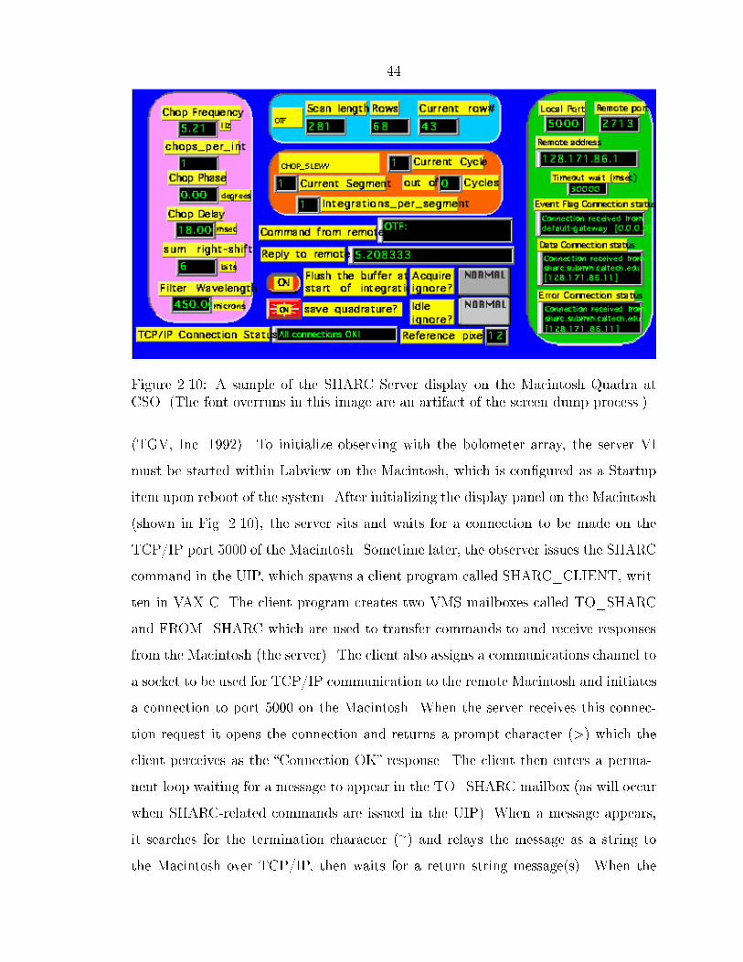
44

Figure 2.10: A sample of the SHARC Server display on the Macintosh Quadra atCSO. (The font overruns in this image are an artifact of the screen dump process.)(TGV, Inc. 1992). To initialize observing with the bolometer array, the server VImust be started within Labview on the Macintosh, which is con�gured as a Startupitem upon reboot of the system. After initializing the display panel on the Macintosh(shown in Fig. 2.10), the server sits and waits for a connection to be made on theTCP/IP port 5000 of the Macintosh. Sometime later, the observer issues the SHARCcommand in the UIP, which spawns a client program called SHARC_CLIENT, writ-ten in VAX C. The client program creates two VMS mailboxes called TO_SHARCand FROM_SHARC which are used to transfer commands to and receive responsesfrom the Macintosh (the server). The client also assigns a communications channel toa socket to be used for TCP/IP communication to the remote Macintosh and initiatesa connection to port 5000 on the Macintosh. When the server receives this connec-tion request it opens the connection and returns a prompt character (>) which theclient perceives as the �Connection OK� response. The client then enters a perma-nent loop waiting for a message to appear in the TO_SHARC mailbox (as will occurwhen SHARC-related commands are issued in the UIP). When a message appears,it searches for the termination character (�) and relays the message as a string tothe Macintosh over TCP/IP, then waits for a return string message(s). When the

45client receives the prompt symbol (>) it stops waiting for further messages from theMacintosh and instead waits for or acts upon the subsequent mailbox message fromother UIP commands.Once the client has connected to the server, the Mac initiates three more TCPconnections to the VAX: one for error messages (through port 5001 on both ma-chines), event �ags (port 5002), and data (port 5003). Multinet is con�gured onthe VAX so that when the Mac sends a connection request to these ports, theappropriate server program will be initiated on the VAX. The connection to port5001 starts the program SHARC_EVENT_FLAG_SERVER, port 5002 starts theSHARC_ERROR_SERVER, and port 5003 starts the SHARC_SCAN_WRITER.All error conditions on the Mac are sent to the error server process on the VAX andappear as messages on the UIP operator's terminal. The event �ag channel is usedto clear the backend wait (BEWAIT) status on UIP observing commands when theMac has gathered the appropriate number of data. Finally, data are sent to the scanwriter process along with some header variables when appropriate.2.4.4 Data display on the MacintoshThe two main data acquisition modes for bolometer observing at CSO are the scan-ning mode (known as OTF_MAP) and the pointed observation mode (known asCHOP_SLEWY). Both modes involve the use of the CSO's chopping secondary.2.4.4.1 OTF_MAPThe term OTF_MAP (�on-the-�y� mapping) refers to the observing mode in whichthe antenna computer directs the telescope to scan across the source at a constantrate, usually in azimuth at a rate of a few arcseconds per second, while data is gathered�on-the-�y�. Because rapid sampling of the lock-in signal allows for the best possiblesky noise subtraction, we sample after each chop period of the secondary mirror whichis the maximum rate possible. This method allows extended maps to be constructedmore rapidly than with a series of pointed observations. The raw signal is sampled

46by the A/D system at 1 kHz and sent to the DSP via a �ber optic link. Performingdigital lock-in detection, the DSP demodulates the data with a sine wave templatefunction and reports a signal level at the chopping rate. The demodulated bolometersignals are displayed in real time on the Macintosh in the form of 24 separate stripchart graphs (see Fig. 2.11). The basic display is modeled on the �Display Data�module written by Kevin Boyce of GSFC. As integrations are obtained they are sentback to the VAX over Ethernet in real time. The data are accumulated at the socketon the VAX and written to disk all at once at the end of each row of the map. Thisstrategy has the advantage of requiring only a single open and close of the data �lefor each OTF_MAP row. The data consist of 4 byte integers in DSP units. The dataheader of each scan contains the scale factor for the proper conversion from DSP unitsto millivolts. The conversion from DSP units to actual voltage (post-ampli�cation)is: V (volts) = �DSP units32� 106 ��fc��750T �2s�6 (2.21)where f is the chopping frequency in Hz, c is the number of chop cycles per integration(usually 1), T is the unitless amplitude of the sine wave template (defaults to 750),and s is the right shift (in bits) applied to the data by the DSP (defaults to 6). Thechopping frequency is generated on the DSP board in the Macintosh in the form of a0 to 5 volt square wave and can take on quantized values satisfying the equation:f(Hz) = 1000n where 2 � n � 512: (2.22)The chopper throw is determined by the ampli�cation and o�set applied to the squarewave signal by the chopping secondary control circuitry built by Martin Houde atCSO. Currently, the throw must be tuned manually. However, a simple closed-loopcircuit has been designed and is being built that will interface with the I/O board inthe Macintosh to enable it to automatically set and monitor the chopper throw (viathe standard UIP command SECONDARY on the VAX).

47Figure 2.11: This scan of Jupiter is a sample of the SHARC OTF mapping display on the Macintosh Quadra at CSO. Thelarge sweep auto-scales with the signal from the reference pixel while the grid of 24 sweeps shows the signals from the entirearray on the same scale. The graphical layout of the display was originally conceived by Kevin Boyce at NASA Goddard.

482.4.4.2 CHOP_SLEWYThe term CHOP_SLEWY refers to the standard pointed observation combining twomotions: constantly chopping the secondary mirror (at a few Hz) while frequentlynodding the telescope (every few seconds) to move the target source between thepositive and negative beams and provide better subtraction of atmospheric �uctua-tions and beam asymmetries. As in OTF_MAP mode, the demodulated bolometersignals are displayed on the Macintosh as strip charts. Upon the completion of eachnodding segment, data are sent to the VAXStation which immediately appends it tothe current �le. At the conclusion of the speci�ed number of chopping cycles, the av-erage and RMS value of the data in each channel are written to the �le after the scandata. Since the multiplex advantage of a (continuum) linear array is best exploited inmapping mode, the pointed observing mode of SHARC was not fully-commissioneduntil August 1996. It is expected to be used more in the future for deep integrationson point sources.2.5 Data reductionSince all demodulated SHARC data are stored on the VAX, it is most convenient forthis machine to run the data reduction software. Using the NOD-2 dual beam restora-tion algorithm (Haslam 1974; Emerson, Klein & Haslam 1979), Darek Lis has writtenan OTF data reduction program called CAMERA. The program interactively pro-ceeds through the various steps of data reduction: 1) pixel-to-pixel gain calibration,2) automatic or manual de-spiking, 3) de-striping, 4) constant o�set or linear baselineremoval, 5) airmass correction, 6) dual beam restoration, 7) azimuth/elevation point-ing correction, and 8) transformation to equatorial celestial coordinates. In standardmode, images of the source are created by restoring a map from each pixel of the arrayseparately. A separate mode of the software is available for automatically analyzingpointing scans and pixel gain scans. In a separate FORTRAN program called RE-GRID, the restored images written by CAMERA are summed together into a regular

49grid in equatorial coordinates with sigma-weighting and �ux calibration applied. Theoutput image �le from REGRID is in FITS format (Wells, Greisen & Harten 1981)and can be read into a variety of software packages.2.5.1 Pixel gain calibrationBecause of small di�erences in the thermal properties of each pixel and in the opticale�ciency across the focal plane, each pixel of the bolometer array exhibits a slightlydi�erent level of response when centered on a given source. Although the magnitudeof the e�ect is generally less than 10% in the SHARC pixels, it is a good practice tomeasure and remove it from the data. The relative gains of the pixels are measured atthe CSO by scanning a bright planet quickly through the array such that atmosphericchanges are minimal during the scan. This is accomplished with elevation scansinvoked by the UIP command OTF/SIDEWAYS. The planet is placed in the positivebeam for several scans followed by the negative beam for several scans. Each scan isanalyzed in the gain mode of CAMERA which writes out a �le with the computedgains normalized to unity. These gains are then averaged to create the gain �le namedCAMERA.DAT to be subsequently used in data reduction.2.5.2 DespikingCosmic ray hits and static electronic glitches are occasionally manifest in the dataas temporal spikes in the scans. Spikes may appear in a single pixel or in all pixelsat once. Fortunately, these spikes can be automatically identi�ed and �agged inCAMERA by their magnitude with respect to the RMS background level. The valueof the spike is replaced by the average of four values: the two adjacent integrationsfrom that pixel and the integration from the two adjacent pixels (if they are notalready �agged). An avoidance range can be speci�ed within which spikes will not beremoved by the automatic procedure. Alternatively, spikes can be �agged manuallyin CAMERA.

502.5.3 DestripingAfter despiking, any correlated noise remaining on the array appears as stripes in thescan data along the direction of the array. On nights of unstable or windy conditions,the dominant source of correlated noise originates above the telescope. Most likely thecorrelation is due to cells of water vapor blowing through the two beams faster thanthe chopping period (� 0:25 seconds). Removal of these stripes is a riskier processthan despiking, especially when extended emission is present. For this reason, anavoidance region in the scan can be speci�ed in CAMERA within which the datawill not contribute to the calculation of the destriping correction and within whichno destriping correction will be made. This feature enables one to ensure that thestructure of speci�ed sources will not be altered by this noise reduction algorithm.2.5.4 O�set or baseline removalDuring long scans, a drift in the signal zero level may occur. Although this e�ect isusually not detectable in SHARC scans, CAMERA allows the removal of a constanto�set or a baseline computed from a speci�ed number of integrations on each end ofthe scan. Of course, if destriping has already been invoked, no o�set should remainat this point.2.5.5 Airmass correctionEven in excellent conditions on Mauna Kea, the zenith optical depth of the atmo-sphere � at 350 and 450�m is always greater than 0.5. (This optical depth � corre-sponds to an emissivity � = 0:39 via the relation: � = 1 � e�� ). As a source risesand sets, the airmass A(t) through which it is observed changes, causing the signalstrength S(t) to rise and fall signi�cantly as a function of time t:S(t) = S0 exp [�A(t)� ] where A(t) = sec [zenith angle(t)]; (2.23)

51where S0 is the signal that would be recorded above the atmosphere. In order toproperly calibrate the continuum �ux density of all the sources observed, it is essentialto measure the optical depth each night, preferably on several sources observed atmany di�erent airmasses. Once the optical depth has been computed, the scans ofeach source can be calibrated to a �xed airmass with CAMERA before summing intoa map.2.5.6 Dual beam restorationOnce the scans are calibrated, they can be restored from a dual beam response patterninto a single beam sky intensity. This is accomplished in CAMERA with the NOD2libraries. The raw dual beam scan is essentially a derivative of the sky intensity. Therestoration process uses the edges of the scan as a zero level which is propagatedacross the scan (introducing some additional noise) in order to properly reconstructthe extended emission. Both before and after the restoration, the scans are writtento GREG format RGDATA �les named CAMERA.DUAL and CAMERA.REST.2.5.7 Pointing correctionOccasionally it necessary and valid to correct the pointing o�sets listed in the scanheader. For example, if the pointing is not rechecked after a change in reference pixel,the operator may have erred in the sign of the change to the �xed zenith angle o�setof the telescope. Or, a thermal pointing shift of the telescope may have occurredsince the most recent pointing scan. Because the OTF scans are recorded in azimuth-elevation coordinates, these telescope-based pointing shifts can be corrected in datareduction after the observation. The o�sets to shift the image should be speci�ed inCAMERA as the direction you wish the image to move in azimuth and elevation.2.5.8 Coordinate transformationAfter restoration, each integration of each scan is transformed by CAMERA fromazimuth-elevation coordinates to celestial equatorial coordinates using the appropriate

52header information of the local sidereal time and telescope o�sets. Space exists inthe raw data �le header for individual motor encoder readings, but these are notcurrently written by the antenna computer. The data are treated as if the telescopewas pointed at the requested location during the scan. The transformed integrationsare then output to the �le CAMERA.RADEC.2.5.9 Regridding, summing and �ux calibrationMultiple maps of a given source (in the form of multiple CAMERA.RADEC �les)can be summed by the program REGRID. A center position in right ascension anddeclination and a grid of pixels about that point must be speci�ed. Each integrationof each map is placed into the appropriate pixel and added in with sigma weighting.Each map can be given an absolute �ux calibration conversion from millivolts (mV)to Jy which will be applied individually. The �ux calibration changes smoothly withopacity, with larger opacities causing fewer mV per Jy. Like the optical depth, it isvital that the �ux calibration be computed for each night at some consistent referenceairmass (typically 1.0). In REGRID, additional pixels can be �agged in any or allmaps if necessary. The pixel-to-pixel gain calibration can also be invoked at this pointif it has not already been applied. The output of REGRID is a FITS image. At theCSO, smoothing and customized display of these images is achieved in the GRAPHICpackage developed at the Insitut de Radio Astronomie Millimétrique (IRAM).2.5.10 CHOP_SLEWY data reductionA software package called the Bolometer Array Data Analysis Software has beendeveloped by Dominic Benford to read, sum, display and calibrate data obtained inCHOP_SLEWY mode. The command line interface resembles the CLASS packagedeveloped at IRAM for heterodyne spectroscopy.

532.6 SensitivityFinally, this chapter concludes with a demonstration of the sensitivity achieved withSHARC at the telescope in the case of short and long integrations.2.6.1 Short integrationsShown in Fig. 2.12 are SHARC OTF scans taken with the same pixel (22) understable atmospheric conditions on 27 April 1996. With calibration based on Uranus,the NEFD achieved in a one second integration on blank sky adjacent to the planetis 3.8 Jy at 350�m and 2.2 Jy at 450�m. These values are about a factor of �ve abovethe most optimistic background limits computed in Eq. 2.18 and 2.19.2.6.2 Long integrationsIn order to test the camera sensitivity during long integrations, it is necessary toconsider a series of data taken during constant sky conditions. The longest integrationperformed to date with SHARC is the CSO deep �eld survey for protogalaxies whichcontains the sum of 1,007,270 0.244-second pixel integrations. This corresponds to4370 seconds of integration in each 1000 resolution element in the map. Thereforethe RMS noise achieved in the �nal map (95 mJy at 450�m) implies an averageNEFD = 6:2 Jy=pHz, However, these data are spread over a large �eld (30) andacquired over many nights with varying weather conditions and may not represent thee�ective NEFD for long integrations on a single position with the CHOP_SLEWYmode.Because the CHOP_SLEWY observing mode mode was only recently commis-sioned, no comprehensive sensitivity measurements exist yet. However, we can con-struct long OTF integrations by adding together scans from di�erent pixels overadjacent patches of sky during the same map; thereby insuring that the data aretaken during similar sky conditions. For this purpose we use a map of Uranus for in-trinsic calibration and use only those scans which do not pass near the planet (> 2500

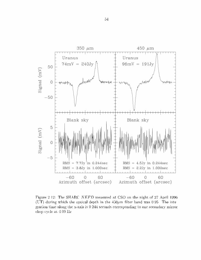
54

Figure 2.12: The SHARC NEFD measured at CSO on the night of 27 April 1996(UT) during which the optical depth in the 450�m �lter band was 0.95. The inte-gration time along the x-axis is 0.244 seconds corresponding to one secondary mirrorchop cycle at 4.09 Hz.

55away). A plot of the RMS noise versus integration time on the blank sky in this mapis shown in Fig. 2.13. For the timescales probed by these data, the decrease of inte-

Figure 2.13: The RMS noise in a single SHARC pixel is plotted as a function ofintegration time at 450�m. The data at the upper left come from raw dual beamscans of Uranus taken within the same hour. The solid square at the right marksthe RMS noise achieved in the �nal restored map of the deep �eld survey. The opensquare represents the estimated noise prior to single beam restoration.grated noise with time closely follows the theoretical prediction. Representing a muchlonger integration time, the deep �eld point lies above the trend, partly due to addednoise from the dual beam restoration process (explained further in section 2.5.6) andpartly due to the fact that the data were taken during varying weather conditions.

56Chapter 3 Submillimeter Continuum Images ofUCHII Regions3.1 The characteristics of interstellar dustOver the past decade, the development of large infrared and submillimeter telescopesalong with sensitive detectors has allowed astronomers to measure thermal emissionfrom cool interstellar clouds. Composed primarily of invisible molecular hydrogengas, these clouds can be studied only through emission from other molecules or dust.Contrary to many common spectral lines from molecular species, thermal dust emis-sion has an optical depth of much less than one at wavelengths longer than 200�m inmost interstellar clouds (Hildebrand 1983). Hence the total submillimeter continuum�ux density is proportional to the number of grains present in the telescope beam.With instruments like the Submillimeter High Angular Resolution Camera (SHARC)at the CSO, the spatial distribution of dust can now be mapped at high resolution.However, the determination of the mass of dust from �ux density measurements de-pends critically on the far-infrared emissivity of dust grains. Thus in order to quantifythe physical conditions of dust in interstellar clouds it is necessary to understand thecomposition and shape of individual grains and how they respond to incident ra-diation. For this purpose, a brief review of cosmic dust grains is presented in thefollowing subsections.3.1.1 Dust compositionThe shape and composition of interstellar dust grains have been inferred from astro-nomical observations and laboratory measurements of their probable constituents. Areview of the observed extinction from dust at UV to FIR wavelengths is given by(Mathis 1990). The detailed composition of grains, such as the presence or absence of

57ice mantles, likely varies between di�erent types of regions. To explain the bulk of theobservations, standard ingredients in dust grain models of the interstellar medium in-clude graphite and silicate particles. One of the early and often-quoted models of dustincludes a mixture of six di�erent materials: graphite, silicon carbide (SiC), enstatite([Fe,Mg]SiO3), olivine ([Fe,Mg]2SiO4), iron and magnetite (Fe3O4) (Mathis, Rumpl& Nordsieck 1977, hereafter referred to as MRN). In order to calculate the extinctiondue to a spherical grain of a given material, one must know the complex indices ofrefraction at each wavelength considered. Of the six materials listed, graphite ex-hibits the additional complexity of anisotropic refraction. The geometry of graphiteis described by two axes in the basal plane with a third axis (the c-axis) perpendicularto this plane. The refractive indices for light with the electric �eld (E-vector) parallelto the c-axis (�k) are di�erent from that for light with the E-vector perpendicular tothe c-axis (�?) (Taft & Philipp 1965; Tosatti & Bassani 1970). Although no rigoroustheory exists for computing the optical cross sections of such a material, the commonapproximation (as in the MRN model) is to assume that 1/3 of the grains exhibit�k and 2/3 exhibit �?. In general, the response of a grain to incident radiation ismodeled with the dipole approximation, as the grain radius a . 0:1�. (Note that thisapproximation likely fails in the inner parts of protostellar and protoplanetary accre-tion disks.) The result of the MRN model for both spherical and cylindrical grainsis that of the six materials, graphite is present in all the mixtures which provide thebest �t to the observed interstellar extinction in di�use clouds from UV wavelengthsto 1�m. The required distribution of grain sizes follows the power law distributionn(a) / a�3:5 over the range 0:005�m to � 0:25�m.3.1.2 Dust extinction in the infraredThe extinction predictions of the MRN graphite-silicate grain mixture have beencomputed and extended to longer wavelengths. In a comprehensive paper, Draine& Lee (1984) compiled the dielectric properties of graphite and silicate dust grainsincluding the scattering and absorption cross sections as a function of wavelength

58from 0:03 � 1000�m. They �nd that the MRN model matches the observed near-infrared extinction of di�use clouds with graphite grains (mostly the �? component)contributing a factor of several more extinction than the silicate grains. At longerwavelengths (8 � 50�m), silicate grains dominate the extinction, particularly in the9.7 and 18�m bands in which absorption features have been con�rmed observationally(Dyck & Simon 1977). By 70�m, extinction due to graphite grains (mostly the �kcomponent) again exceeds silicate grains. Draine & Lee (1984) predict the 100�mthermal emission from the MRN mixture and show that it matches the IRAS �uxdensity observed toward clouds of infrared cirrus (Low 1984). Thus the MRN mixturehas proved to be successful in predicting dust extinction and thermal emission acrossthe infrared range.3.1.3 Dust extinction in the submillimeterAt submillimeter wavelengths, the extinction from both graphite and silicate grainsincreases as a power-law with frequency (�),�extNH2 / ��; (3.1)where NH2 is the column density of molecular hydrogen gas. In the model of Mathis,Mezger & Panagia (1983), graphite grains exhibit � = 1:9, silicate grains exhibit� = 2:3, and a mixture of the two yields � = 2:25. Draine & Lee (1984) predict � =1:9 for both species. Recent laboratory measurements of millimeter-wave absorptionin silicate grains yield values of � between 1.5 and 2.5 (Agladze et al. 1996). Theessential reason for this steep drop in extinction is that as the wavelength becomesmuch larger than the radius, the dust grain becomes a poor radiator. Purcell (1969)notes the correspondence of this e�ect to the di�culty of constructing an e�cientbroad-band long-wavelength radio antenna of small size. The absorption e�ciency Qof a grain is de�ned as the ratio of the absorption cross section �abs to the projected

59geometric area: Q � �abs�a2 : (3.2)Often, �abs is re-written in terms of a mass opacity coe�cient � and the grain massdensity � assuming spherical grains:Q = mgrain��a2 = 43�a3���a2 = 43a��: (3.3)A simple derivation of the expected power law drop-o� of the absorption e�ciency ofa grain is given by Knacke & Thomson (1973) and Wright (1982) using formulae fromvan de Hulst (1957) for small ellipsoids. In this derivation, Q can be approximatedby the expansion:Q = �4�Im��� 1�+ 2�� 415�3Im���� 1�+ 2�2��2 + 27� + 382�+ 3 ��+ 8�43 Re��� 1�+ 2�2(3.4)where � = 2�a�=c; a is the particle radius, � is the complex index of refraction, and� is the frequency. The �rst term represents the Rayleigh absorption cross sectionwhich dominates in the low frequency limit. In a dissipative model of atomic os-cillators where the restoring force is proportional to velocity, the imaginary part ofthe dielectric constant is proportional to �. With another factor of � coming from�, the emissivity Q is then proportional to �2 (Andriesse 1974). This relation canbe expected to hold for frequencies lower than the structural resonant frequencies ofthe grains which are generally above 3000 GHz (Gezari, Joyce & Simon 1973). Mea-surements of the emissivity of interstellar grains as a function of frequency should becompared to the expected value of � = 2 derived here.3.1.4 Measurements of dust emissivity in the submillimeterDespite the expected value of � = 2, measurements of � at submillimeter wavelengthsexhibit a broad range from � 1 to over 3 (Helou 1989). Why is there such a variation?

60One explanation for objects with low values of � is that the emission comes from very�ne grains in which surface vibration modes dominate the bulk vibration modes, lead-ing to � = 1 (Seki & Yamamoto 1980). Laboratory measurements con�rm this resultfor grains of olivine, obsidian and fused quartz with a . 0:01�m (Koike, Hasegawa& Hattori 1987). A possible explanation for the values of � > 2 is the presence ofice on grains. The absorptivity of ice has been measured from 2.5 to 330�m (Bertie,Labbé & Whalley 1969). At the longest wavelengths, from about 160 to 330�m, theabsorptivity scales as �4, much steeper than the expected value of 2. This dependenceis predicted by a theory of light absorption by the vibrational modes of the crystalin which the density of states and the vibration intensity are both proportional to �2(Whalley & Labbé 1969).The relevance of ice to dust grains was established by the detection in dense cloudsof absorption features at 3.08 (Soifer, Russell & Merrill 1976), 4.67, 6.0 & 6:85�min combination with the silicate band at 9:7�m. These lines have been attributed toice in the form of a mantle surrounding the silicate core of a grain (Tielens 1989).Calculations on olivine, quartz and lunar rocks by Aannestad (1975) show that thepresence of ice mantles of radii & 1:5acore on grains of these materials steepen �to values of 2.9 to 3.5. For this reason, ice mantles have been invoked to explainmeasurements of � > 2 at millimeter wavelengths (Schwartz 1982). The presence ofice is likely to be augmented on colder grains and there is some evidence that � isinversely correlated with dust temperature in dust clouds around HII regions (Gordon1988). A good overview of the optical constants and opacity of ice, organic, metallicand composite grains compiled by Pollack et al. (1994) shows that the expected valueof � varies signi�cantly with the grain material. Thus, the large variation in observedvalues of � may be real and may reveal the underlying composition and physicalcondition of the grains. Also, fractal models of dust grains suggest that the longwavelength absorption of grains depends strongly on their shape and aspect ratio(Wright 1987). Further accurate measurements of � in the submillimeter range (suchas the data presented in this thesis) are necessary to explore these possibilities.

613.2 Computation of dust column density and massfrom submillimeter �ux densityThe general result of the dust models discussed in the previous section is that theemissivity of the grains decreases with decreasing frequency, causing them to emit amodi�ed Planck spectrum. With this information, the �ux density F� at frequency� from a optically-thin cloud of N dust grains at uniform temperature Td with ageometric cross sectional area � can be immediately written (Hildebrand 1983) asfollows: F� = N�Q�B�(Td)D2 = N�Q�D2 2h�3c2[exp (h�=kTd)� 1] ; (3.5)where D is the distance to the source. As seen in Eq. 3.4, Q� / a and thus F� /�a / vgrain, the volume of a single grain. As mentioned in section 3.1.1, a distributionof dust grain radii n(a) / a�3:5 is present in an interstellar cloud. Truncating thisdistribution at al = 0:01�m and au = 0:25�m, the dust model of Mathis, Mezger& Panagia (1983) �nds good agreement with the observed interstellar extinction AVat optical and infrared wavelengths. One can compute a �ux density-weighted meangrain radius �a over this size distribution:�a = R aual an(a)a3daR aual n(a)a3da = R aual aa�3:5a3daR aual a�3:5a3da (3.6)= R aual a0:5daR aual a�0:5da = 13�a1:5u � a1:5la0:5u � a0:5l � (3.7)= 0:103 �m for au = 0:25�m and al = 0:01�m: (3.8)A contour plot of �a as a function of al and au is included in Fig. 3.1.The value of �a can be used as an e�ective grain radius in the formula for �uxdensity. Essentially, a cloud of N identical grains of radius �a would emit the same�ux density asN grains having the speci�ed power-law distribution of radii. Assumingspherical grains, one can then compute the total �ux density-weighted volume of dust

62

Figure 3.1: Mean �ux density-weighted grain radius for the n(a) / a�3:5 grain dis-tribution as a function of the lower-cuto� radius al and the upper-cuto� radius au.The points labelled MRN and MMP correspond to the models of Mathis, Rumpl &Nordsieck (1977) and Mathis, Mezger & Panagia (1983), respectively.

63in the cloud V = Nvgrain = 4N��a3=3: (3.9)This relation can be used to eliminate N from Eq. 3.5 and arrive withV = Md� = 4��a3=3��a2 F�D2B�(Td)Q� ; (3.10)where � is the grain mass density. The total mass of a cloud with �ux density F�becomesMd = 4�a�3 F�D2B�(Td)Q� ; (3.11)MH2 = 4R�a�3 F�D2B�(Td)Q� ; (3.12)= 1:3� 104Q�J�(Td)� �a0:1�m�� �3 g cm�3�� R100��F�Jy�� Dkpc�2� �GHz��3 M�;(3.13)where R is an empirically-determined gas to dust mass ratio and J� � [exp(h�=kTd)�1]�1. Using the telescope beam size , this equation can be rewritten in terms of thegas column densityNH2 = MH2mH2D2 (3.14)= 8:1� 1017Q�J�(Td)� �a0:1�m�� �3 g cm�3�� R100��F�Jy�� �GHz��3 cm�2:(3.15)By applying the following empirical expression for Q� valid at submillimeter andlonger wavelengths (Hildebrand 1983),Q� = 7:5� 10�4� �2:4 THz�� (3.16)

64the formulas for column density and mass become:NH2 = 7:8� 1010J�(Td) � �a0:1�m�� �3 g cm�3�� R100��F�Jy�� �2:4 THz��3�� cm�2; (3.17)MH2 = 1:3� 10�3J�(Td) � �a0:1�m�� �3 g cm�3�� R100��F�Jy�� Dkpc�2� �2:4 THz��3�� M�:(3.18)In reality, a distribution of dust temperatures will be present in a star-forming cloudwith the warmest grains lying near the young embedded stars and coolest grains lyingin the outer parts of the cloud (in the absence of external heating sources). For thisreason, we cannot expect to be able to �t the entire infrared through submillimeterspectrum with a modi�ed Planck function of a single temperature. Multi-temperaturemodels have been constructed to �t the continuum spectra of star-forming dust cores(Hobson & Padman 1994; Xie et al. 1993; Gürtler et al. 1991; Pajot et al. 1986).These models include a component of small, warm grains (T � 200K) which signif-icantly increase the emission in the 12 and 25�m bands of IRAS. As discussed laterin section 3.10.4, radiative transfer models indicate a smooth distribution of temper-ature with cloud radius (Goldreich & Kwan 1974; Scoville & Kwan 1976). However,because the bulk of the luminosity from UCHII regions emerges at � > 60�m, accu-rate estimates of the dust mass can be obtained by �tting only the cold componentof dust. Measurements at 100, 350/450, 800 and 1300�m are essential to characterizethis component of the spectrum. Many 1300�m �ux density measurements of UCHIIregions exist in the literature (e.g., Chini et al. 1986), and low resolution 100�mdata are available from the IRAS database. IRAS images of UCHII regions are pre-sented in the next section, followed by new high resolution submillimeter images inthe subsequent sections.

653.3 HIRES IRAS imagesIn order to link the new submillimeter images presented in this thesis to the far-infrared, analysis of the IRAS database was undertaken. With the ultimate goal ofspatially resolving the dust surrounding UCHII regions, I conducted a HIRES sur-vey of 75 �elds surrounding the UCHII regions in the Wood & Churchwell surveyalong with others from the literature. A NASA Astrophysics Data Program (ADP)grant was obtained in order to pursue the research. The HIRES algorithm employsthe maximum correlation method to enhance the spatial resolution of IRAS imagesbeyond the standard IRAS Sky Survey Atlas (ISSA) plates, which have 40 to 50 resolu-tion, and approach the di�raction limit of the telescope (Aumann, Fowler & Melnyk1990). The processed �elds are one square degree in size with 1500 pixels, at thewavelengths of 100, 60, 25, and 12�m. The images were analyzed using the Skyviewsoftware package developed at the NASA Infrared Processing and Analysis Center(IPAC). The e�ective resolution achieved by HIRES is approximately 9000 at 100�mand 5000 at 60�m with signi�cant variation from �eld to �eld. Aperture photometrywas performed on the 126 sources in these �elds which could be identi�ed with radio-detected UCHII regions. The list of these sources, together with their measured IRAS�ux densities (within a 20 radius of the centroid) and blackbody color temperaturesbetween 60 and 100�m are given in Table 3.1.In general, the FIR emission remains unresolved at the two longest wavelengthsdespite the improved resolution of the HIRES maps. In a few cases, includingG45.12+0.13 & G45.07+0.13, G75.84+0.40 & G75.78+0.34, and K3-50A & K3-50C,the FIR �ux has been resolved between a pair of adjacent UCHII regions. This allowsmore accurate blackbody �ts when combined with submillimeter data. However, theoverall lack of real detail in the HIRES images emphasized the need for higher resolu-tion submillimeter studies at CSO. As a sample of the HIRES results, contour plotsof the sources later imaged with SHARC are included as Figs. 3.2 through 3.14. Allof the maps are in presented in equatorial (B1950) coordinates.

66Table 3.1: UCHII regions analyzed with HIRES processingCoordinates (1950.0) IRAS �ux density (Jy) TcolSource R.A. Dec. 100�m 60�m 25�m 12�m KW3(OH) 02h21m34.s0 61�5202500 35249 26140 10792 1274 54G133.947+1.064 02h23m15.s5 61�3805700 12569 9828 752 100 57G138.30+1.56 02h57m36.s2 60�1702400 1376 1002 291 55 53G139.909+0.197 03h03m31.s3 58�1900400 1441 1267 504 73 60G206.543-16.35 05h39m09.s3 -01�5704000 30326 18085 12485 1299 49MONR2IRS2 06h05m21.s0 -06�2202500 20652 17649 5072 634 59G189.03+0.784 06h05m40.s8 21�3102800 2924 2097 470 145 53G188.949+0.915 06h05m52.s6 21�3805800 1745 1233 269 78 53G188.793+1.030 06h06m06.s6 21�5101300 1288 1141 268 77 60G189.876+0.516 06h06m21.s8 20�4000500 2592 2063 291 128 57I06068+2030 06h06m53.s9 20�3005000 1456 1240 208 102 59GGD12-15 06h08m24.s1 -06�1100800 4975 3721 726 63 55G192.584-0.041 06h09m59.s3 18�0001600 6247 4647 701 237 55G240.31+0.07 07h42m45.s1 -24�0002400 780 613 64 2 54NGC6334A 17h16m58.s9 -35�5200000 26543 21731 3433 694 59NGC6334B 17h16m58.s9 -35�5103000 22187 19198 3081 765 60NGC6334C 17h17m15.s0 -35�4801500 22783 18924 6215 1325 59NGC6334D 17h17m27.s3 -35�4703000 21220 19089 6201 1226 62NGC6334E 17h17m33.s5 -35�4201500 23743 19177 2798 458 57NGC6334F 17h17m33.s5 -35�4201500 24239 20944 2786 480 60G351.78-0.54 17h23m21.s6 -36�0604400 17607 9720 392 86 46G1.13-0.11 17h45m33.s3 -28�0002900 9320 4396 921 223 42G5.48-0.24 17h56m00.s0 -24�2002500 2082 1537 260 47 53AFGL 5425 17h56m52.s9 -23�4501200 1950 1766 269 38 62G5.89-0.39 17h57m27.s8 -24�0305700 21735 15872 2664 330 53G6.55-0.01 17h57m46.s4 -23�2002600 3604 2581 276 59 53AFGL 5176S 17h58m53.s2 -23�5804100 3146 2430 275 112 55

67Coordinates (1950.0) IRAS �ux density (Jy) TcolSource R.A. Dec. 100�m 60�m 25�m 12�m KG7.47+0.06 17h59m11.s9 -22�2800200 3339 1499 227 108 42G8.14+0.23 18h00m00.s2 -21�4801500 6451 5137 957 171 57G5.97-1.18 18h00m37.s6 -24�2203600 10135 15407 5470 808 102G9.62+0.19 18h03m15.s9 -20�3105200 7617 4620 403 63 48G8.67-0.36 18h03m18.s6 -21�3704300 5122 2338 198 33 42I18035-2126 18h03m36.s9 -21�2601300 916 730 79 30 57G10.47+0.03 18h05m41.s1 -19�5202600 9895 4754 190 36 42G10.30-0.15 18h06m00.s2 -20�0601100 11251 11119 2742 402 66G10.15-0.34 18h06m25.s7 -20�1905600 26177 22250 6109 1013 59G9.876-0.750 18h07m21.s4 -20�4505200 3541 1898 134 134 46G10.62-0.38 18h07m30.s6 -19�5602500 21222 13024 582 83 48G11.110-0.399 18h08m34.s4 -19�3102300 3327 1443 271 105 41I18089-1837 18h08m57.s3 -18�3605600 1785 1545 283 57 60G12.21-0.10 18h09m45.s8 -18�2502600 5125 3199 236 41 50G12.68-0.18 18h11m00.s2 -18�0104900 6542 3382 302 56 44G11.95-0.03 18h11m04.s0 -18�5402500 4275 2399 274 10 46G13.19+0.04 18h11m10.s6 -17�2901900 4417 3625 667 152 59G12.81-0.20 18h11m18.s0 -17�5601900 31018 22339 3166 329 53G13.87+0.28 18h11m42.s5 -16�4603000 5657 4402 753 141 55G12.91-0.26 18h11m44.s3 -17�5300300 6425 3569 331 29 46G13.21-0.15 18h11m54.s7 -17�3303300 2518 1134 84 14 42I18134-1652 18h13m26.s9 -16�5103100 4795 4140 648 175 60G10.841-2.592 18h16m13.s0 -20�4804800 3802 3305 533 116 60G15.04-0.68 18h17m26.s7 -16�1404600 19560 23149 4451 835 77G16.94-0.07 18h19m05.s8 -14�1405100 2633 1149 207 109 41G18.146-0.284 18h22m13.s3 -13�1703400 9859 9779 1798 390 66G18.302-0.391 18h22m52.s3 -13�1200400 3355 2270 440 53 51G19.491+0.135 18h23m14.s3 -11�5402300 2556 1465 158 36 46

68Coordinates (1950.0) IRAS �ux density (Jy) TcolSource R.A. Dec. 100�m 60�m 25�m 12�m KG19.07-0.27 18h23m58.s9 -12�2800700 5785 4486 521 105 55G19.61-0.23 18h25m04.s6 -11�5400900 1025 498 30 12 42G20.08-0.14 18h26m12.s9 -11�2600800 507 310 21 12 48G20.99+0.09 18h26m17.s9 -10�3600900 1645 1237 130 31 55G23.70+0.17 18h31m08.s7 -08�0903900 2841 2101 354 58 55G24.47+0.49 18h31m28.s4 -07�2002100 7218 6052 1231 296 59G25.650+1.050 18h31m39.s2 -06�0200600 2696 1097 220 82 41G23.96+0.15 18h31m42.s1 -07�5700900 4053 3550 670 89 60G23.43-0.21 18h32m03.s3 -08�3503900 9680 6022 572 130 50G23.87-0.12 18h32m30.s6 -08�0900900 1922 1574 139 39 59I18328-0735 18h32m50.s0 -07�3505100 3848 2358 183 48 48I18341-0727 18h34m09.s7 -07�2702100 5297 3202 304 71 48G25.72+0.05 18h35m22.s0 -06�2701100 4211 3006 367 78 53G25.38-0.18 18h35m29.s1 -06�4901100 12834 13875 3493 506 71G26.54+0.42 18h35m34.s3 -05�3202000 2180 1855 336 99 59G26.10-0.07 18h36m29.s4 -06�0901100 1841 1287 112 30 53G27.28+0.15 18h37m54.s9 -05�0003000 1963 1037 96 22 44G27.49+0.19 18h38m08.s9 -04�4704500 2542 2001 219 48 57G28.198-0.050 18h40m19.s9 -04�1700000 3953 2031 199 27 44I18406-0338 18h40m38.s0 -03�3803000 2872 2261 290 77 57G28.288-0.364 18h41m38.s1 -04�2100000 3918 3456 977 101 60G28.60-0.36 18h42m10.s2 -04�0403000 1968 1305 138 43 51G29.96-0.02 18h43m27.s0 -02�4205100 12937 11832 2169 330 62G30.53+0.02 18h44m25.s0 -02�1003200 1503 1404 156 25 64G31.41+0.31 18h44m58.s5 -01�1600800 2013 775 50 -6 39G30.78-0.02 18h45m01.s0 -01�5803200 23611 25105 5750 1073 69G31.28+0.06 18h45m37.s5 -01�2903800 3638 1703 134 16 42G32.15+0.13 18h46m58.s9 -00�4103300 1243 766 169 30 50

69Coordinates (1950.0) IRAS �ux density (Jy) TcolSource R.A. Dec. 100�m 60�m 25�m 12�m KG31.396-0.257 18h46m59.s5 -01�3203800 3392 2297 311 53 51G32.80+0.19 18h47m18.s0 -00�2204500 523 328 43 8 50G33.133-0.092 18h49m25.s0 00�1100000 1839 1274 199 49 51G33.91+0.11 18h50m18.s0 00�5104500 3165 1827 275 45 48G34.26+0.14 18h50m46.s0 01�1100000 28752 18686 2291 342 50G35.57+0.06 18h53m31.s0 02�1901300 3024 1397 186 87 42G35.578-0.030 18h53m52.s0 02�1604300 4661 2990 323 106 50G37.55-0.11 18h57m46.s4 03�5901500 3706 2288 275 92 50G35.200-1.741 18h59m14.s1 01�0804800 15612 13366 2309 380 60G37.874-0.399 18h59m23.s7 04�0803000 6266 4276 465 122 51G41.52+0.04 19h04m40.s0 07�3401500 1585 763 132 69 42G41.71+0.11 19h04m49.s0 07�4800000 1017 499 114 58 44G42.46-0.26 19h07m27.s0 08�1403300 2941 1698 269 99 48W49N 19h07m49.s6 09�0103400 30782 21796 3135 481 53G43.237-0.045 19h08m01.s7 09�0101900 6219 3439 258 90 46G43.795-0.127 19h09m30.s6 09�3004000 2761 1893 213 61 51G43.18-0.52 19h09m46.s0 08�4701100 1903 1064 196 77 46G45.12+0.13 19h11m06.s0 10�4803000 7603 7668 1742 350 68G45.48+0.13 19h11m46.s8 11�0701500 4562 3805 472 100 59G45.45+0.06 19h12m01.s0 11�0400000 8539 7188 1120 184 59G43.89+0.14 19h12m03.s7 09�1702600 1873 1082 262 78 48I19139+1113 19h14m00.s3 11�1305900 1102 736 71 28 51G48.609+0.027 19h18m11.s7 13�4903800 6956 5330 570 154 55G50.31+0.68 19h19m11.s0 15�3802900 1214 774 149 57 50G53.605+0.046 19h28m09.s6 18�1400400 2594 1372 142 98 44G54.10-0.06 19h29m31.s8 18�3601900 3390 1848 261 101 46G60.884-0.128 19h44m14.s8 24�2802000 5855 4585 820 159 57G61.48+0.09 19h44m40.s8 25�0500700 13897 13575 1841 279 66

70Coordinates (1950.0) IRAS �ux density (Jy) TcolSource R.A. Dec. 100�m 60�m 25�m 12�m KK3-50A 19h59m50.s8 33�2402200 14386 14444 2391 516 68G69.540-0.975 20h08m09.s8 31�2204100 3516 1536 105 27 41G78.438+2.659 20h17m53.s0 40�4700600 3864 3223 765 130 59G75.84+0.40 20h19m48.s3 37�2102900 8376 9045 2004 699 71G75.78+0.34 20h19m50.s9 37�1602900 9418 7297 891 150 55G76.18+0.10 20h22m05.s6 37�2802900 2143 1474 189 50 51G76.38-0.621 20h25m33.s8 37�1205000 14281 14353 3479 496 68G79.321+1.291 20h26m20.s2 40�4201500 4972 4743 915 193 64G77.965-0.006 20h27m47.s3 38�5101600 4251 3702 716 150 60G79.297+0.281 20h30m42.s8 40�0600400 11715 14800 2103 398 82G106.80+5.31 22h17m41.s1 63�0304200 14064 12105 1641 347 60G109.872.11 22h54m17.s8 61�4505000 22544 15473 961 27 51G110.209+2.630 22h55m07.s3 62�2104000 4068 3157 324 148 55NGC7538S 23h11m36.s6 61�1105000 16882 13554 2554 432 57G111.612+0.374 23h13m19.s2 60�5100300 3724 3168 779 112 59G111.282-0.663 23h13m54.s6 59�4503800 2977 2286 402 98 55I23139+5939 23h13m58.s5 59�3902300 1208 624 111 45 44Average 54

71

Figure 3.2: HIRES processed IRAS maps of G19.61-0.23. Contour levels are 1, 2, 5,10 to 100 by 10% of the peak intensity in each 1� �eld (12�m: 4073; 25�m: 13956;60�m: 35728.9; 100�m: 20081.9 MJy/sr).

72

Figure 3.3: HIRES processed IRAS maps of G29.96-0.02. Contour levels are 1, 2, 5,10 to 100 by 10% of the peak intensity in each 1� �eld (12�m: 5516; 25�m: 37686;60�m: 71062; 100�m: 25276 MJy/sr).

73

Figure 3.4: HIRES processed IRAS maps of G34.26+0.14. Contour levels are 1, 2, 5,10 to 100 by 10% of the peak intensity in each 1� �eld (12�m: 7651; 25�m: 19003;60�m: 85429; 100�m: 77272 MJy/sr).

74

Figure 3.5: HIRES processed IRAS maps of G45.1+0.1. The two UCHII regionsG45.12+0.13 and G45.07+0.13 have been resolved. Contour levels are 1, 2, 5, 10 to100 by 10% of the peak intensity in each 1� �eld (12�m: 10794; 25�m: 34889; 60�m:66149; 100�m: 24283 MJy/sr).

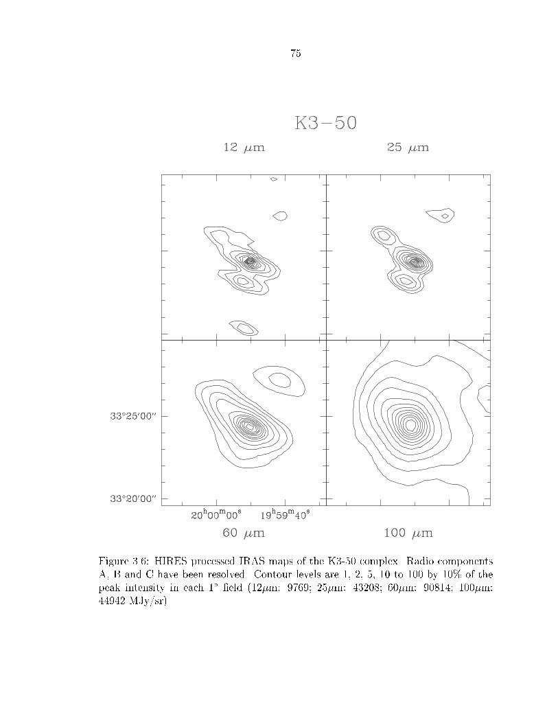
75

Figure 3.6: HIRES processed IRAS maps of the K3-50 complex. Radio componentsA, B and C have been resolved. Contour levels are 1, 2, 5, 10 to 100 by 10% of thepeak intensity in each 1� �eld (12�m: 9769; 25�m: 43208; 60�m: 90814; 100�m:44942 MJy/sr).

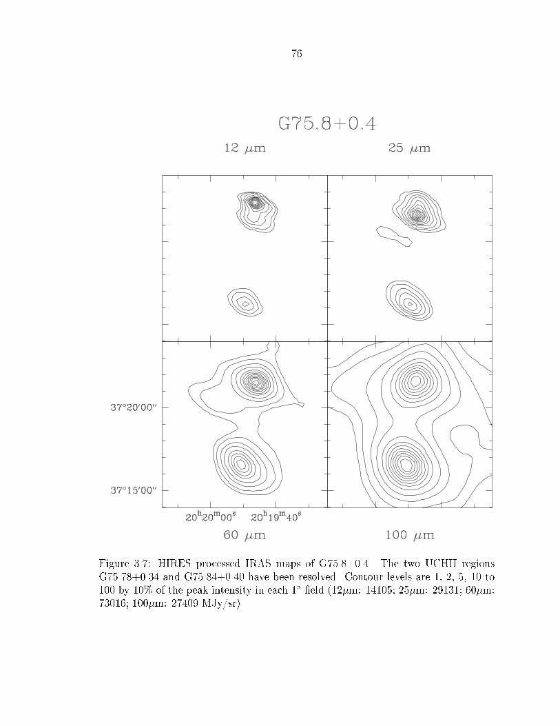
76

Figure 3.7: HIRES processed IRAS maps of G75.8+0.4. The two UCHII regionsG75.78+0.34 and G75.84+0.40 have been resolved. Contour levels are 1, 2, 5, 10 to100 by 10% of the peak intensity in each 1� �eld (12�m: 14105; 25�m: 29131; 60�m:73016; 100�m: 27409 MJy/sr).

77

Figure 3.8: HIRES processed IRAS maps of W3(OH). Contour levels are 1, 2, 5, 10to 100 by 10% of the peak intensity in each 1� �eld (12�m: 11259; 25�m: 116263;60�m: 111077; 100�m: 59204 MJy/sr).

78

Figure 3.9: HIRES processed IRAS maps of G138.30+1.56. Contour levels are 1, 2,5, 10 to 100 by 10% of the peak intensity in each 1� �eld (12�m: 465; 25�m: 6986;60�m: 8224; 100�m: 5102 MJy/sr).

79

Figure 3.10: HIRES processed IRAS maps of G139.909+0.197. Contour levels are 1,2, 5, 10 to 100 by 10% of the peak intensity in each 1� �eld (12�m: 522; 25�m: 9455;60�m: 7928; 100�m: 3207 MJy/sr).

80

Figure 3.11: HIRES processed IRAS maps of Monoceros R2. Contour levels are 1,2, 5, 10 to 100 by 10% of the peak intensity in each 1� �eld (12�m: 10093; 25�m:83071; 60�m: 109584; 100�m: 58851 MJy/sr).

81

Figure 3.12: HIRES processed IRAS maps of GGD12-15. Contour levels are 1, 2, 5,10 to 100 by 10% of the peak intensity in each 1� �eld (12�m: 993; 25�m: 24816;60�m: 33049; 100 �m: 25241 MJy/sr).

82

Figure 3.13: HIRES processed IRAS maps of the S255 complex. The extension tothe southwest of the �eld center coincides with S256. Contour levels are 1, 2, 5, 10 to100 by 10% of the peak intensity in each 1� �eld (12�m: 3101; 25�m: 11339; 60�m:26675; 100�m: 15907 MJy/sr).

83

Figure 3.14: HIRES processed IRAS maps of G240.31+0.07. Contour levels are 1, 2,5, 10 to 100 by 10% of the peak intensity in each 1� �eld (12�m: 54.8; 25�m: 2140;60�m: 7580; 100�m: 4032 MJy/sr).

843.4 Calibration and pointing accuracy of the SHARCimagesThe data reduction scheme used to prepare the SHARC images was described inChapter 2. Before presenting and interpreting the images, a discussion of the �uxcalibration, dynamic range and pointing accuracy should be considered.3.4.1 Flux calibrationThe absolute �ux calibration of ground-based submillimeter continuum observationsis ultimately limited by the stability and uniformity of the atmosphere. Even onrelatively calm nights, the zenith optical depth � across the frequency band of the �ltercan change signi�cantly (� 20%) on short timescales (minutes to hours). Beyond theregular increase with airmass, � can be a signi�cant function of azimuth and elevationdepending on the position of clouds and weather systems. The most accurate methodof measuring � through the desired �lter is to record the signal strength of a sourceas it rises or sets through di�erent airmasses. By nature, this measurement requiresseveral hours during which � can be changing. In the 350 and 450�m bands, � � 1 ingood weather. Thus a 20% change in � will cause � 20% change in the signal strength.The calibration conversion factor from volts to Janskys depends on the signal recordedfrom a standard source including planets and secondary sources previously calibratedto planets (e.g., Sandell 1994), taking into account the fact that planetary brightnesstemperatures vary as a function of frequency (Hildebrand 1985; Orton et al. 1986). Soif � changes by 20% between the observation of the calibrator and the observation ofthe source, then the source �ux density will be in error by � 20% plus the additionalmeasurement uncertainties. Several scans of the source taken at di�erent times andinterspersed with the calibrator can help reduce this uncertainty. If the source isextended spatially, the extended �ux has additional uncertainty because the responseof the telescope beam to an extended source di�ers from the response to a pointsource. The best estimate of the accuracy of the �ux calibration on a given night can

85be made from the dispersion in several measurements of � on di�erent sources. Thefrequent readings from the CSO 225 GHz � -meter can also be considered (if it wasoperating dependably at the time). With these e�ects, the �ux calibration of a singleOTF map recorded in one session is probably no better than 30% accurate. Since theimages in the following sections were constructed from a sum of 1, 2 or 3 maps, theestimated calibration accuracy is � 30%.3.4.2 Dynamic rangeDue to the presence of sidelobe response in the 350 and 450�m beams, there is adynamic range limit for genuine features surrounding bright sources in the SHARCmaps. As can be seen in the 350�m beammap in Fig. 2.8, the brightest feature outsidethe central beam lies at the � 4% intensity level. Consistent results have been foundwith maps of bright compact galaxies such as Arp 220. When several maps taken atdi�erent parallactic angles are summed, the e�ect of the sidelobes will tend to smearwhich will raise the dynamic range further. Thus the dynamic range is at least 25:1.All of the sources identi�ed in the maps presented in the following sections easily fallwithin this criterion. It should be noted that the beam is signi�cantly cleaner at 450�than at 350�m (due to the telescope surface accuracy) and hence the dynamic rangein maps at the longer wavelength is nearly a factor of 2 larger.3.4.3 Pointing accuracyThe CSO is an altitude-azimuth mount telescope. Pointing correction is accomplishedwith two sets of o�sets in this coordinate system: tilt terms which vary as a function ofelevation, and �xed terms which remain constant (in the ideal case) and vary only dueto small di�erences in the mounting position of the selected instrument. Additionalcorrections in azimuth and elevation result from a formula containing several constantsdesigned to account for deviations between the radio and optical pointing of thetelescope. These so-called �optical pointing constants� are periodically measured andupdated using an optical telescope attached to the radio telescope backing structure

86and looking through a hole in the primary. Finally, a signi�cant refraction correction(. 10) to the elevation angle is computed from the current humidity reading. Thedetails of these formulas will not be discussed, but they provide an idea of the levelof complexity required in the pointing of a submillimeter telescope.Even when these systematic terms correct well for pointing errors, other e�ectscan disturb the pointing accuracy of the telescope. Thermal changes at sunset andsunrise can cause small distortions in the telescope surface which cause � 1000 changesin the �xed terms. For this reasons, observations during these times cannot be reliedupon for absolute pointing accuracy. The best pointing accuracy is achieved when the�xed terms are measured on a calibrator located near the target source in both axesof motion, particularly in elevation. Unfortunately, in the 350 and 450�m wavebands,very few bright point-like sources exist. Planets of small angular size (< 1000) such asUranus, Neptune and (much of the time) Mars are best. Nearby evolved stars withdust shells and well-known positions (such as IRC+10216) are also good pointingsources. Bright star-forming regions with a dominant component of compact emissionhave also been used by assuming the submillimeter emission peak coincides withinfrared or radio positions (Sandell 1994). UCHII regions have been used for thispurpose, even though the presence of extended emission and the lack of a prioriknowledge of the submillimeter position makes them less reliable pointing sources.Because UCHII regions themselves are the subject of this work, I chose to useonly sources with the most reliable peak positions (Uranus, IRC+10216, Orion KL,IRAS16293-2422 and K3-50A) for correction of the �xed pointing terms. For thisreason, the angular distance between the pointing source and the target source wasin many cases larger than recommended (> 90� in azimuth or > 20� in elevation).The absolute pointing accuracy of a single map is estimated to be �500. For manyof the regions studied, more than one map was acquired and summed, which shouldimprove the accuracy of the peak positions of sources in the map.

873.5 SHARC images of cometary UCHII regionsSince the installation of SHARC at CSO in September 1995, over a dozen UCHII re-gions have been imaged at 350 and/or 450�m. The sample includes regions of variousradio morphology. The cometary UCHII regions studied are G19.61-0.23A, G29.96-0.02, G34.3+0.2, G45.12+0.13, and GGD12-15. Similar to the cometary shape is theclassic blister-type HII region Monoceros R2 (Mon R2). The shell-like or spher-ical UCHII regions studied are W3(OH), K3-50A and K3-50C. Also studied area group of UCHII regions unresolved at radio wavelengths including G45.07+0.13,G138.300+1.558, G139.909+0.197, G240.31+0.07 and a group of sources in the S255complex. The �nal object presented is the G75 complex which contains several UCHIIregions of cometary and core-halo shapes. These sources will be discussed individ-ually in the following sections with the exception of the two G45 sources which arepresented in greater detail in Chapter 5. Also, prior to the installation of SHARC,maps of 800�m emission from many of these UCHII regions were made at the CSOwith the single channel bolometer equipped with a 2000 Winston cone. These mapsare included in the following sections. Although most of the sources are unresolvedat the limited signal to noise level of these maps, they do provide 800�m �uxes whichare used in the greybody models computed in section 3.9. All of the maps in thefollowing sections are in presented in equatorial (B1950) coordinates.3.5.1 G34.3+0.2 Complex (W44, AFGL 2271, I18507+0110)At a distance of 3.8 kpc (Kuchar & Bania 1994), G34.25+0.14 is a 9000 (1.7 pc) ex-tended, shell-like HII region as seen in Fig. 3.15 (Fey et al. 1994; Fey et al. 1992). Justbeyond the northwest edge of the extended HII region lies the prototypical cometaryUCHII region G34.26+0.14 (see Fig. 3.16). The discovery of this source promptedspeculation that the cometary tail was due to relative motion of the central ionizingsource with respect to the interstellar medium (Reid & Ho 1985). Higher sensitivityobservations show that the tail is at least 1500 (0.28 pc) in length and that it curvesback on itself (Gaume, Fey & Claussen 1994). Theoretical models propose that this

88

Figure 3.15: 2.0 cm radio continuum image of the G34.3+0.2 complex reproducedfrom Fig. 2 of Fey et al. (1994).kind of cometary shape could be explained if the young O star was moving at a rateof 10-20 km s�1 through the natal molecular cloud (Mac Low et al. 1991; Van Buren& Mac Low 1992). Also, two unresolved radio components labelled �A� and �B� lie300 southeast and 200 northeast of the cometary region �C�, respectively. The locationof the OH masers (Garay, Reid & Moran 1985) and the primary concentration ofH2O masers (Benson & Johnston 1984; Downes et al. 1979) lie between the 3 radiocomponents directly opposite to the direction of the cometary tail. VLA images ofthe NH3(3,3) and (1,1) inversion transitions indicate a concentration of dense gas in-timately associated with the H2O masers (Heaton, Little & Bishop 1989; Keto 1987)reaching densities of � 7� 107 cm�3 in the central region (Garay & Rodríguez 1990).Such high densities are con�rmed by the presence of a CH3CN core (Akeson & Carl-strom 1996). Maser emission has also been observed in the 325 (51;5 ! 42;2), 439(64;3 ! 55;0) and 471 GHz (64;2 ! 55;1) transitions of H2O (Melnick et al. 1993).In a JCMT 330-360 GHz spectral line survey, 14 transitions of ethanol have beendetected indicating a rotational temperature of 125 K and a large column density(2� 1015 cm�2) consistent with grain surface chemistry (Macdonald, Habing & Mil-lar 1995). Observed with the Berkeley-Illinois-Maryland Array (BIMA) millimeter

89

Figure 3.16: 2.0 cm radio continuum image of G34.26+0.14 reproduced from Fig. 1of Gaume, Fey & Claussen (1994).interferometer, the position of the complex molecules in the region also lies a fewarcseconds east of the UCHII region (Mehringer & Snyder 1996). Together, these ob-servations suggest that the UCHII region expands preferentially to the west away fromthe dense molecular gas. Additional H2O maser spots lie at an o�set (�4000;+1800)from the UCHII region (Fey et al. 1994) and probably trace a separate center of starformation activity at a projected distance of 0.8 pc.Shown in Fig. 3.17 are 350�m and 450�m images of the G34.3+0.2 complex.The position of the cometary UCHII region is marked by a triangle and the twosites of H2O maser emission are marked by crosses. Essentially, the dust emissionpeaks on the UCHII region. The half power width of the dust core is 3400 (0.63 pc),identical to the size of the CS J=5!4 emission mapped with the IRAM 30m telescope(Churchwell, Walmsley & Wood 1992). Extensions of dust emission protrude to thesouthwest and northwest bracketing the ionized tail of the cometary UCHII regionon a large scale. The dust clump northwest of the UCHII region coincides withthe secondary concentration of H2O masers (Fey et al. 1994). Blueshifted 13COemission near this position was once interpreted as an extension of an out�ow fromthe UCHII region (Matthews et al. 1987) but the coincidence of the dust clump and

90

Figure 3.17: Bottom panel: 350�m image of G34.3+0.15 (d = 3:8 kpc) with theposition of the UCHII region marked by the triangle, and the two H2O maser con-centrations marked by crosses. The contour levels are 25, 30, 40, 50, 60, 80, 100,150, 250, 350, 450 and 550 Jy/beam. Top panel: 450�m image of the same regionwith contour levels 8, 10, 12, 14, 16, 18, 20, 25, 30, 40, 50, 60, 90, 120, 150 and 180Jy/beam. The asterisks mark the position of the submillimeter sources identi�ed inTable 3.2.

91masers provides overwhelming evidence that it is a separate core. Two additionaldust sources (G34.3+0.2SE and G34.3+0.2SW) lie to the southeast and southwestof the UCHII region. There is no compact radio continuum nor maser emission atthese positions. However, the �ux in these objects imply large molecular masses, 1700and 560 M�, respectively (see Table 3.2). Thus they may contain younger massiveprotostars forming on the outskirts of the dust core containing the UCHII region.Table 3.2: Observed properties of the dust clumps toward G34.3+0.2Src UCHII o�set B1950.0 Coordinates S350�m S450�m Mgas# (��00,��00) R.A. Dec. Jy Jy M�1 (0; 0) 18h50m46:s1 +01�1101000 1060 410 65002 (�33;�27) 18h50m43:s9 +01�1004400 300 96 17003 (�40;+18) 18h50m43:s5 +01�1102900 260 90 15004 (+42;+17) 18h50m48:s9 +01�1102800 170 55 9405 (+42;�76) 18h50m48:s9 +01�0905400 83 39 5606 (+5;�57) 18h50m46:s5 +01�1001300 51 35 440Sum of 6 clumps 1900 730 11500Total emission 4700 1700 27000To con�rm the protostellar nature of the isolated continuum source G34.3+0.2SE,a map of the H2CO (31;2 � 21;1) transition at 225.6777 GHz around its positionwas obtained with the CSO (see Fig. 3.18). Emission in this transition indicatesa high volume density of molecular gas (Wang et al. 1995; Mangum & Wooten 1993).G34.3+0.2SE (clump 5 in Table 3.2) was chosen because it is su�ciently separatedfrom the UCHII region to avoid confusion in the 3000 CSO beam at this frequency.The position of an H2CO core coincides with the 350=450�m source, con�rming thepresence of a dense star-forming molecular core associated with the dust core. Thespectrum closest to the peak is shown in Fig. 3.19. The core of emission on thenorthwest edge of the map originates from the vicinity of the UCHII region.3.5.2 G29.96-0.02 (W43S, AFGL 2245, I18434-0242)At a distance of 7.4 kpc (Churchwell, Walmsley & Cesaroni 1990), G29.96-0.02 isa cometary UCHII region similar in appearance to G34.26+0.14. The main radiocomponent lies on the edge of a shell-like envelope about 800 (0.3 pc) in diameter

92

Figure 3.18: H2CO 31;2� 21;1 map integrated over the velocity range 53 to 62 km s�1of the submillimeter dust clump that lies southeast of G34.3+0.2 (d = 3:8 kpc) inFig. 3.17. The position of the dust clump is marked by the asterisk. Contour levelsare 2.5 to 5.0 by 0.5 K km s�1 on the main beam brightness temperature scale.(Megeath et al. 1990; Cesaroni et al. 1994). As seen in Fig. 3.20, di�use radio emissionextends up 4000 (1.4 pc) to the north where a faint �lament about 16 (0.6 pc) in lengthturns toward the west (Fey et al. 1995). Another �lamentary structure emerges fromthe southern edge of the shell and extends 1000 to the east.The 800�mCSO single channel bolometer map shows a compact dust core (Fig. 3.21).The total FIR (IRAS) luminosity of the dust core is 106:30L� (Wood & Churchwell1989).Strong emission from the molecular species CH3CN, CS and 13CO is present to-ward the core. Observed with an 1100 beam at the IRAM 30m telescope, the half

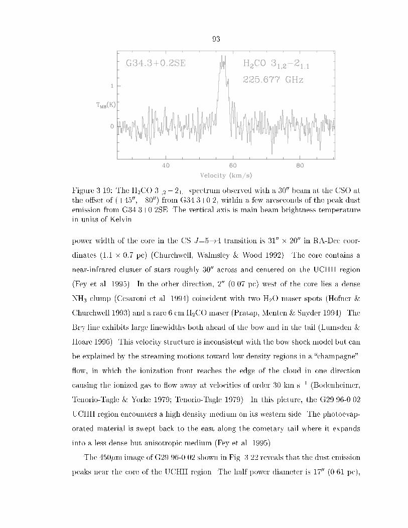
93

Figure 3.19: The H2CO 31;2� 21;1 spectrum observed with a 3000 beam at the CSO atthe o�set of (+4500;�8000) from G34.3+0.2, within a few arcseconds of the peak dustemission from G34.3+0.2SE. The vertical axis is main beam brightness temperaturein units of Kelvin.power width of the core in the CS J=5!4 transition is 3100 � 2000 in RA-Dec coor-dinates (1:1 � 0:7 pc) (Churchwell, Walmsley & Wood 1992). The core contains anear-infrared cluster of stars roughly 3000 across and centered on the UCHII region(Fey et al. 1995). In the other direction, 200 (0.07 pc) west of the core lies a denseNH3 clump (Cesaroni et al. 1994) coincident with two H2O maser spots (Hofner &Churchwell 1993) and a rare 6 cm H2CO maser (Pratap, Menten & Snyder 1994). TheBr line exhibits large linewidths both ahead of the bow and in the tail (Lumsden &Hoare 1996). This velocity structure is inconsistent with the bow shock model but canbe explained by the streaming motions toward low density regions in a �champagne��ow, in which the ionization front reaches the edge of the cloud in one directioncausing the ionized gas to �ow away at velocities of order 30 km s�1 (Bodenheimer,Tenorio-Tagle & Yorke 1979; Tenorio-Tagle 1979). In this picture, the G29.96-0.02UCHII region encounters a high density medium on its western side. The photoevap-orated material is swept back to the east along the cometary tail where it expandsinto a less dense but anisotropic medium (Fey et al. 1995).The 450�m image of G29.96-0.02 shown in Fig. 3.22 reveals that the dust emissionpeaks near the core of the UCHII region. The half power diameter is 1700 (0.61 pc),

94

Figure 3.20: 2.0 cm radio continuum image of G29.96-0.02 reproduced from Fig. 2 ofFey et al. (1995).slightly smaller than the CS core. But as in G34.26+0.14, an extended componentof dust emission lies along the general direction of the ionized cometary tail to theeast and also to the north along the extended radio �lament. Looking back at the800�m map (Fig. 3.21), the faint clump of emission in the east matches the northeasttail of emission seen in the 450�m image. The coincidence of the extended radioand submillimeter continuum suggests that there exists a di�use component of warmdust associated with the expanding HII region. The di�use 450�m emission to thesouthwest is not identi�ed with any radio continuum emission.

95

Figure 3.21: 800�m image of G29.96-0.02. Contour levels are 6 to 30 by 3 Jy/beam.The position of the UCHII region is marked by the cross (Wood & Churchwell 1989).

96

Figure 3.22: 450�m image of G29.96-0.02 (d = 7:4 kpc). Contour levels are 5, 10 to100 by 10 Jy/beam. The position of the UCHII region is marked by the triangle andthe direction of the cometary �laments are indicated by arrows (Fey et al. 1995).

973.5.3 G19.61-0.23 (I18248-1158)G19.61-0.23 is a compact cluster of 5 UCHII regions (see Fig. 3.23), the most promi-nent of which is component A, a cometary UCHII region associated with strong H2Omaser emission (Churchwell, Walmsley & Cesaroni 1990). The UCHII regions liewithin a compact core of 800�m continuum emission as seen in the CSO single chan-nel bolometer map in Fig. 3.24. At a distance of 4.5 kpc (Wood & Churchwell 1989),the total FIR (IRAS) luminosity of the region is 105:42L� (Wood & Churchwell 1989).

Figure 3.23: 6 cm VLA radio continuum image of G19.61-0.23 reproduced from Wood& Churchwell (1989).

98

Figure 3.24: 800�m image of G19.61-0.23. Contour levels are 8 to 40 by 4 Jy/beam.The position of radio component A is marked by the triangle (Wood & Churchwell1989).The position angle of the cometary radio tail of component A is 60� as indicatedby the arrow on the SHARC 450�m image in Fig. 3.25. Analogous to G34.26+0.14and G29.96-0.02, the radio position of the main UCHII region is consistent with thepeak dust position with a slight extension of dust along the radio tail. In this case,all �ve radio components lie within the 20 Jy contour.

99

Figure 3.25: 450�m image of G19.61-0.23 (d = 4:5 kpc). Contour levels are 6, 8, 10,15, 20 to 70 by 10 Jy/beam. The position of the �ve UCHII components are markedby letters (Wood & Churchwell 1989).

1003.5.4 GGD12-15 complex (I06084-0611)GGD12-15 is a cluster of Herbig-Haro objects identi�ed from the Palomar Sky Survey(Gyulbudaghian, Glushokov & Denisyuk 1978). A large molecular out�ow originatingfrom these objects was �rst identi�ed in the CO J=1!0 transition by Rodríguez,Cantó & Torrelles (1982). A cometary UCHII region (see Fig. 3.26) powered by aB0.5 star lies at the core of GGD12-15 with a water maser located � 3000 (0.15 pc)to the northeast (Tofani et al. 1995). OH maser emission has also been detected inthis region (Rodríguez et al. 1980) along with a core of NH3 with a molecular gasmass of � 100M� (Torrelles et al. 1983). Despite higher resolution CO J=2!1 mapsobtained at the James Clerk Maxwell Telescope (JCMT), the powering source of themolecular out�ow remains uncertain (Little, Heaton & Dent 1990) but the out�owaxis lies closer to the H2O maser source than the UCHII region. Although the UCHIIregion dominates the FIR emission, it does not have a prominent counterpart in thenear-infrared. At a distance of 1 kpc (Rodríguez, Cantó & Torrelles 1982), the FIRand submillimeter luminosity of the entire region is 104:15L� (Little, Heaton & Dent1990).

Figure 3.26: A 3.6 cm VLA image of GGD12-15 reproduced from Tofani et al. (1995).

101An 800�m JCMT map peaks on the UCHII region with some extended emissionsurrounding the H2O maser position. A cluster of near-infrared sources lies aroundthe lower contours of the submillimeter emission including the 200L� source 9Mcoincident with the H2O maser (Harvey et al. 1985). With higher angular resolutionthan the JCMT map, the 350�m SHARC image of GGD12-15 reveals a distinct sub-peak of emission at the position of the maser source (see Fig. 3.27).

Figure 3.27: 350�m image of the GGD12-15 complex (d = 1 kpc). Contour levelsare 10 to 35 by 5 Jy/beam. The positions of the H2O maser and UCHII region aremarked (Tofani et al. 1995).Matching an extended 20�m source (Harvey et al. 1985), the main submillimeterpeak occurs a few arc seconds northwest of the UCHII region, in front of the cometaryhead of ionized gas. As in G34.3+0.2, the absolute pointing of the SHARC image

102is strengthened by the good correspondence of the H2O maser and the sub-peak ofcontinuum emission. Hence the magnitude and direction of the o�set from the UCHIIregion is likely to be real. This o�set supports the model of cometary UCHII regions(discussed in section 3.5.1) as the result of a streaming motions in an asymmetricmedium. As in G29.96-0.02 and G19.61-0.23, faint extended dust emission lies alongthe direction of expansion of the HII region.3.5.5 Monoceros R2 complex (I06053-0622)At a distance of 830 pc (Henning, Chini & Pfau 1992), Mon R2 is a re�ection neb-ulosity containing a blister-type UCHII region (see Fig. 3.28) imaged at the VLAby Massi, Felli & Simon (1985). Early FIR observations revealed a young clusterof infrared sources with a total FIR luminosity of 104:70L� (Beckwith et al. 1976;Thronson et al. 1980). Infrared polarimetric studies have been performed (Hodapp1987; Aspin & Walther 1990). More sensitive near-infrared observations revealed theionizing source to be IRS1SW, consistent with a B0 star (Howard, Pipher & Forrest1994). The infrared cluster is associated with a core of dense gas identi�ed in mapsof the CS J=5!4 and 2!1 transitions (Heyer et al. 1986) and in NH3 (Torrelles etal. 1983). A gas kinetic temperature of 55 K was derived from observations of theNH3 (1,1) and (2,2) transitions in a 4000 beam, (Takano 1986).The brightest near-infrared source in the cluster is IRS3, a pre-main sequenceobject undetected in radio continuum or in Br emission. VLA observations pinpointan H2O maser coincident with IRS 3 (Tofani et al. 1995). Previously, H2O maseremission was detected at another location o�set (�3400;+1700) from IRS3 (Rodríguez& Cantó 1983) but this source was not detected in the more recent observations ofTofani et al. (1995). IRS3 has been resolved into two components at near-infraredwavelengths including a conical re�ection nebula 500 AU in length and a possiblecircumstellar disk (Koresko et al. 1993). A giant molecular out�ow 280 (6.8 pc) inextent has been mapped in CO J=1!0 (Wolf, Lada & Bally 1990). Due to the largedimensions of the out�ow, it is unclear whether IRS1SW, IRS3 or some other source is

103the source of the out�ow. High resolution CS and 13CO observations indicate denseclumps in the out�ow (Tafalla, Bachiller & Wright 1994).

Figure 3.28: 6 cm radio continuum image of Mon R2 reproduced from Fig. 1 of Massi,Felli & Simon (1985).An early submillimeter map at 870�m with 1800 (0.072 pc) resolution obtained atthe Swedish ESO Submillimeter Telescope (SEST) revealed seven dust clumps in theMon R2 cluster (Henning, Chini & Pfau 1992) which were interpreted as remnantsof star formation. The SHARC 350�m image of Mon R2 is shown in Fig. 3.29. Thepeak emission occurs southeast of the UCHII region whose cometary tail expandsto the northwest along a minimum ridge in the dust emission. As in the case ofG34.3+0.2 and GGD12-15, the con�dence in the absolute pointing accuracy of theSHARC map is better than 300 judging by the good correspondence of the H2O maser(coincident with IRS3) and the sub-peak of continuum emission. Thus the magnitudeand direction of the o�set from the UCHII region is signi�cant and strongly con�rms

104

Figure 3.29: 350�m image of the Mon R2 complex (d = 0:83 kpc). Contour levelsare 10 to 52 by 2 Jy/beam. The arrow marks the expansion direction of the blisterUCHII region whose cometary peak is marked by the triangle (Massi, Felli & Simon1985). The squares mark the position of the two H2O masers (Tofani et al. 1995;Rodríguez & Cantó 1983), the eastern one being coincident with IRS3. The asterisksmark the position of submillimeter sources identi�ed in Table 3.3.

105the blister model for the HII region. In addition to the two main sources, a dozenother dust clumps surround the cloud core. Some of the clumps can be identi�edwith the Henning, Chini & Pfau (1992) sources. A list of source positions and �uxesis compiled in Table 3.3. Some of the sources have no infrared counterpart in a deepK-band image of the region (Carpenter 1996). As this is the nearest UCHII regionin the survey, the complex submillimeter structure evident here suggests that similarstructure may be present (but unresolved) in the submillimeter images of the moredistant sources.Table 3.3: Observed properties of the dust clumps in Mon R2Src O�set� B1950.0 Coordinates S350�m Mgas# ��00;��00 R.A. Dec. Jy M�1 �55;�31 06h05m17:s9 �06�2205900 49 112 �56;�3 06h05m17:s8 �06�2203100 39 93 �42;�45 06h05m18:s8 �06�2301300 74 164 �24;+19 06h05m20:s0 �06�2200900 61 135 �17;�14 06h05m20:s5 �06�2204200 98 226 0;�3 06h05m21:s6 �06�2203100 92 207 +3; 42 06h05m21:s8 �06�2104600 56 128 �24;�63 06h05m20:s0 �06�2303100 36 89 �9;�51 06h05m21:s0 �06�2301900 36 810 +28;+11 06h05m23:s5 �06�2201700 44 1011 �61;+40 06h05m17:s5 �06�2104800 30 712 �50;+58 06h05m18:s3 �06�2103000 26 613 +18;�49 06h05m22:s8 �06�2301700 26 614 +45;+31 06h05m24:s6 �06�2105700 29 615 �14;+64 06h05m20:s6 �06�2102400 30 716 �77;+69 06h05m16:s5 �06�2101900 28 6Sum of 16 clumps 757 168Total emission 2180 480�O�sets measured from the H2O maser associated with IRS 33.5.6 Summary of cometary UCHII regionsThe dust surrounding cometary UCHII regions is generally extended on arc minutescales. In most cases, the position of the peak dust emission coincides with thedominant compact radio source with extended emission present along the direction of

106the tail. One exception is the blister-type HII region in Mon R2 which clearly expandsasymmetrically from the edge of the dust core of IRS 1 into a cavity relatively empty ofdust. In most sources, additional sub-peaks of dust emission have also been identi�ed,some of which are associated with known H2O maser clusters and some of which areheretofore unknown sources.3.6 SHARC images of shell-like UCHII regions3.6.1 K3-50 complex (I19598+3324)At a distance of 8.7 kpc (Roelfsema, Goss & Geballe 1988), K3-50 is a complexof compact HII regions associated with the W58 molecular cloud (Neugebauer &Garmire 1970). VLA observations with 0:0014 (0.006 pc) resolution of the K3-50 radiocomponents A and C1 reveal shell-type morphologies (Turner & Matthews 1984). Ona larger scale of 500 (0.2 pc), component A shows an ionized bipolar structure withevidence for out�ow in radio recombination lines while components B and D are di�useHII regions roughly 4000 (1.7 pc) in diameter lying to the northeast and southeast,respectively (DePree et al. 1994). The FIR luminosity of the entire region is 106:32L�(Thronson & Harper 1979). By comparing the radio continuum to the infrared Br�line �ux, the visual extinction toward A, B, C1 and C2 has been measured at AV = 15,26, 97 and 32 mag, respectively, averaged over a 1500 aperture (Roelfsema, Goss &Geballe 1988). Component D lies behind only 2 magnitudes of extinction and is visiblein optical images. Component A (VHII = �27:5 km s�1) is likely to be located towardthe front side of the molecular cloud (Wynn-Williams et al. 1977) while componentsB, C1 and C2 (VHII = �21 km s�1) are situated on the far side. In a 500 aperture at thepeak radio position, the extinction toward C1 rises to AV � 190mag, implying a largehydrogen column density in a compact molecular envelope surrounding the ionizingstar. H92� images of K3-50C1 reveal an out�ow of ionized gas from this source(DePree, Rodríguez & Goss 1995). As a whole, component C also corresponds toON 3, an OH maser source (Wynn-Williams, Werner & Wilson 1974). A recent deep

1073.6 cm image of K3-50 (see Fig. 3.30) revealed a new faint, ultracompact componentcalled C58.75, � 1500 (0.63 pc) south of C1 and C2 (DePree 1996). This object maybe coincident with a faint near-infrared source (Howard et al. 1996).D

EC

LIN

AT

ION

(B

19

50

)

RIGHT ASCENSION (B1950)20 00 02 0019 59 58 56 54 52 50 48

33 26 00

25 30

00

24 30

00

23 30

00

22 30

C2 C1

C58.75

B

K3-503.6 cm Continuum

A (core)

D

A (lobes)

K3-50 3.6 cm Radio Continuum

Figure 3.30: VLA 3.6 cm image of the K3-50 complex courtesy of Chris DePree.

108With the exception of component D, all of the radio sources exhibit 800�m con-tinuum emission with component A being the dominant source (see Fig. 3.31). The350�m image of K3-50 in Fig. 3.32 provides a more detailed picture of the dust emis-sion from the HII regions. The brightest dust source is coincident with K3-50A with astrikingly round distribution, con�rming its frequent use as a submillimeter pointingsource (Sandell 1994). Some faint extended emission lies to the northeast near thedi�use HII component B. Another ridge of dust is seen toward components C1 andC2 and brightening toward the south at the newly-discovered radio source C58.75. ACO J=2!1 map taken at the CSO also reveals a molecular out�ow emerging fromthe position of C58.75. These three �ndings indicate that C58.75 is probably theyoungest massive protostar in the region. Fortunately, K3-50A and C are su�cientlyseparated to be resolved in the IRAS HIRES images, shown in Fig. 3.6. Separategreybody model �ts to their spectral energy distribution indicate that component Cis cooler than A (32 K vs. 56 K). Because the dust is heated internally, this tempera-ture di�erence is consistent with the higher extinction measured toward component Cand may indicate that the embedded stars there are younger than those of componentA.

109

Figure 3.31: 800�m image of the K3-50 complex. Contour levels are -5, 5 to25 by 5 Jy/beam. Triangles mark the position of the �ve radio components(A,B,C1,C2,C58.75) labelled in Fig. 3.32.

110

Figure 3.32: SHARC 350�m image of the K3-50 complex. Contour levels are -10, 10,20, 30, 40, 50 to 250 by 50 Jy/beam. The radio continuum components are markedby triangles and labels (DePree et al. 1994; DePree 1996).

1113.6.2 W3(OH) (G133.95+1.06, IC1795)Discovered during the Westerhout (1958) radio survey, W3 is a complex of threeHII regions (Schraml & Mezger 1969). Lying about 150 southeast of the main radiocomponent, W3(OH) is the prototypical shell-type UCHII region (Dreher & Welch1981) with embedded concentrations of OH masers (Reid et al. 1980; Fouquet & Reid1982; Norris, Booth & Diamond 1982) and CH3OH masers (Menten 1992). Evidencefor gravitational infall has been seen in the form of redshifted NH3 absorption features(Keto 1987; Reid, Myers & Bieging 1987). Lying � 700 (0.075 pc) east of the UCHIIregion is a group of 22 GHz H2O masers (see Fig. 3.33) coincident with a faintmillimeter continuum source known as the Turner-Welch (TW) object (Turner &Welch 1984). Maser emission in the 321 GHz (102;9 ! 93;6) transition (Menten,

Figure 3.33: 18 cm radio continuum image of W3(OH) reproduced from Reid &Moran (1988).Melnick & Phillips 1990) and the 183 GHz (31;3 ! 22;0) transition (Cernicharo et

112al. 1990) has also been detected from this source. Frequently dubbed as a massiveprotostar, this (as yet) unresolved object was recently measured to be 43 mJy and< 0:007 (500 AU) in diameter at 87.7 GHz with the BIMA array (Wilner, Welch &Forster 1995).At a distance of 2.2 kpc (Humphreys 1978), the FIR luminosity of W3(OH) isapproximately 105:0L� (Harper 1974; Thronson & Harper 1979). As shown in theCSO 800�m map in Fig. 3.34, the dust emission from W3(OH) peaks at the positionof the UCHII region. However, some contribution of dust emission no doubt comesfrom the TW object. When compared with the 110 GHz IRAM �ux measurement of112 mJy (Wink et al. 1994), the 3 millimeter �ux from the TW object is consistentwith optically-thin dust emission with a submillimeter spectral index � 4, implyinga dust mass in the range of 3 to 60M�. This mass estimate is barely compatiblewith the 60M� C18O clump identi�ed at the same position (Wink et al. 1994). Thedust interpretation is also easily compatible with the upper limit of 1 mJy at 23 GHz(Wilson, Johnston & Mauersberger 1991).Shown in Fig. 3.35, the SHARC image of W3(OH) gives a more sensitive pictureof the region. Similar to an unpublished JCMT 450�m map (Sandell 1994), the350�m dust emission peaks near the UCHII region with noticeable extension towardthe east and northeast. The �ux at the position of the TW object is 295 Jy/beam.Since the TW object is subarcsecond in size, this measurement is an upper limit toits submillimeter �ux. The total angular extent of the dust emission in the region(about 8000, 0.85 pc) matches well with the size of the molecular cloud measured fromVLA H2CO observations (Dickel et al. 1984). The FWHM of the 350�m emissionis 2000 (0.21 pc). As observed with the Kuiper Airborne Observatory (KAO), thedeconvolved FWHM sizes of the FIR emission are 800 and 1300 at 50 and 100�m,respectively (Campbell et al. 1989).An interesting feature is the �lament extending to the northeast which matchesthe shape and location of the NH3 �lament imaged by Wilson, Gaume & Johnston(1993). Although the authors o�er several possible explanations for the �lament, wenote that the feature is analogous to the �lamentary structures seen in C18O emission

113

Figure 3.34: 800�m image of W3(OH). Contour levels are 6, 8, 10 to 40 by 5 Jy/beam.The position of the UCHII region is marked by the triangle (Dreher & Welch 1981)and the TW object is marked by the cross (Turner & Welch 1984).in the Ophiuchus complex (de Geus & Burton 1991) and to the �laments emergingfrom the core of Orion A seen in both molecular line (Tatematsu et al. 1993) andcontinuum emission (Wiseman & Ho 1996; Lis et al. 1996). The nature of these�laments remains unclear though they seem to be common in molecular clouds.3.6.3 Summary of shell-like UCHII regionsAs is the case in the cometary UCHII regions, the dust surrounding the shell-likeUCHII regions is concentrated about the position of the radio sources. Elongationsin the dust cores match the distribution of the compact sources. Lower level dustemission also comes from the more di�use HII regions in the vicinity of the compactsources.

114

Figure 3.35: 350�m image of W3(OH) (d = 2:2 kpc). Contour levels are -15, 15, 30,60, 120, 180, 240 to 600 by 120 Jy/beam. The position of the UCHII region and TWobject are marked (Turner & Welch 1984). A �lament of dust emission matches theNH3 imaged at the VLA by Wilson, Gaume & Johnston (1993).

1153.7 SHARC images of unresolved UCHII regions3.7.1 G240.31+0.07 (I07427-2400, FIRSSE 223)At a distance of 6.6 kpc, G240.31+0.07 was discovered to be a H2O maser source withthe E�elsberg 100-m telescope (Henning et al. 1992). Subsequently, it was found toexhibit broad CO J=1!0 line wings and a 8.4 GHz point source with a �ux consistentwith a B0.5 star (McCutcheon et al. 1995). The total FIR luminosity of the IRASsource is 104:69L�, consistent with an O9 star (Shepherd & Churchwell 1996a). Abipolar molecular out�ow from the UCHII region G240.31+0.07 was resolved in a COJ=1!0 map by Shepherd & Churchwell (1996a). This discovery prompted furtherinterest in this source. The 350�m SHARC image in Fig. 3.36 shows a compact dustcore coincident with the UCHII region.

Figure 3.36: 350�m image of G240.31 (d = 6:6 kpc). Contour levels are -5, 5, 10 to110 by 10 Jy/beam. The triangle marks the UCHII region (McCutcheon et al. 1995).

1163.7.2 G138.295+1.555 & G138.300+1.558 (AFGL 4029, W5East, I02575+6017)The molecular cloud IC1848A lies at the border of the extended HII region S199(W5) at a distance of 3.8 kpc. . Embedded in this cloud are the radio continuumsources G138.295+1.555 and G138.300+1.558 which have been imaged with the VLAKurtz, Churchwell & Wood (1994). In a 4000 beam, H2O maser and NH3 emissionhas been detected from this region (Churchwell, Walmsley & Cesaroni 1990) whichis associated with the infrared cluster Air Force Geophysical Laboratory (AFGL)AFGL 4029 (Price & Murdock 1983). An optical and near-infrared study of thecluster reveals over 30 young B stars, the most massive of which ionizes the UCHIIregion G138.300+1.558 near the center of the cluster (Deharveng et al. 1996). Theluminous (104L�) highly-reddened (AV = 25 � 30 mag) object AFGL 4029-IRS1corresponds to the radio source G138.295+1.555 which is likely to be an ionized stellarwind accompanied by a high velocity optical jet. A CO out�ow is also identi�ed withthis source (Snell et al. 1988).The 350�m SHARC image shows that the bulk of the dust emission is associatedwith G138.295+1.555 and lies in a short ridge that is elongated north-south. Theridge runs perpendicular to the CO out�ow (see Fig. 4.5 in Chapter 4). There is nosigni�cant dust emission at the position of G138.300+1.558 and the near-infrared clus-ter. Apparently, the bulk of the dust lies around the younger source G138.295+1.555,which probably accounts for the H2O maser and NH3 emission as well.

117

Figure 3.37: 350�m image of G138.300+1.558 and G138.295+1.555 (d = 3:8 kpc).Contour levels are 4 to 20 by 2 Jy/beam. The triangles mark the positions of theUCHII regions from Kurtz, Churchwell & Wood (1994).

1183.7.3 G139.909+0.197 (AFGL 437, I03035+5819)AFGL 437 is a compact cluster of a few dozen young stars and a re�ection nebula over3000 (0.3 pc) in diameter in the near-infrared (Weintraub & Kastner 1996). Near thecenter of the cluster lie two UCHII regions imaged with the VLA (Kurtz, Churchwell &Wood 1994) and an H2O maser (Torrelles et al. 1992). H2O maser and NH3 emissionhas been detected by Churchwell, Walmsley & Cesaroni (1990). At a distance of2:0 � 0:5 kpc (Arquilla & Goldsmith 1984), the total FIR (IRAS) luminosity of thecluster is 104:18L�. A wide, apparently poorly-collimated molecular out�ow emergesfrom the center of the cluster (Gómez et al. 1992). From polarimetric imaging ofthe out�ow cavity, Weintraub & Kastner (1996) suggest that the young stellar objectWK 34 (which coincides with the H2O maser position) illuminates the re�ectionnebula and drives the out�ow. In Fig. 3.38, we see that the 350�m emission extendsaround the position of the UCHII region and the WK 34 source with an additionalpeak to the east near the other UCHII region. The further extent of the submillimeteremission may originate from other embedded members in the cluster (Weintraub etal. 1996).

119

Figure 3.38: 350�m image of the G139.909+0.197 complex (d = 2:0 kpc). Thelarge triangle marks the position of the main UCHII region while the smaller trianglemarks a fainter 8.4 GHz source (Kurtz, Churchwell & Wood 1994). The cross marksthe H2O/infrared source WK 34 (Torrelles et al. 1992; Weintraub & Kastner 1996).Contour levels are -8, -6, 6 to 18 by 2 Jy/beam.

1203.7.4 S255 complex (AFGL 896, I06099+1800)Lying at a distance of 2.5 kpc (Mezger et al. 1988), the S255 molecular cloud isassociated with a cluster of red nebulae S254-S257 (Sharpless 1959) with extendedradio continuum emission. Also present in the cloud between two of the extendedHII regions (S255 & S257) are several UCHII regions (see Fig. 3.39) labelled S255-1= G192.584-0.041 (Israel 1976; Rengarajan & Ho 1996) and three fainter � 1 mJysources called S255-2a,b,c (Snell & Bally 1986).

Figure 3.39: 5 GHz VLA image of the S255 molecular cloud complex reproduced fromFig. 11 of Snell & Bally (1986).

121A possible tracer of shocked gas in out�ows, blueshifted OH absorption appearsin front of G192.584-0.041 (Ruiz et al. 1992). Components S255-2b and 2c coincidewith the 20�m sources IRS 1 and IRS 2 (Beichman, Becklin & Wynn-Williams 1979).Associated with S255-2 is a cluster of 32 near-infrared sources all but 2 of whichare invisible on the Palomar Observatory Sky Survey (POSS) plate (Tamura et al.1991). Early FIR and submillimeter maps revealed two peaks separated by � 10 indeclination and coinciding with the two sources S255-1 and S255-2 (Ja�e et al. 1984;Richardson et al. 1985). Higher resolution 1.3 mm continuum maps with the IRAM30-m telescope resolved the dust emission into distinct clumps including a third sourcesouth of the �rst two cores called FIR-3 (Mezger et al. 1988). All three sources areseen in the SHARC image in Fig. 3.40.Also visible in the SHARC image, signi�cant extended emission lies between S255-FIR1 and S255-FIR2. Four extensions of dust match with extensions in the CSJ=7!6 emission of the region shown as indicated by the stars in Fig. 3.41.The S255 region has been studied in detail in the near-infrared by Howard (1996).Shown in Fig. 3.42, is an enlargement about the source S255-FIR2 with the 350�mcontours overlaying a K-band image in greyscale. More than any other, this image in-dicates the great potential of detailed comparison of submillimeter and infrared data.The submillimeter emission locates the raw materials of star formation while the near-infrared emission identi�es the embedded young stellar objects. The main structureat 350�m is a bowl-like feature extending to the northeast. In the near-infrared, thecentral core region of S255-FIR2 shows a limb-brightened shell of molecular hydrogenemission centered on the central core with an additional enhancement of emissionalong the lane of re�ection nebulosity that extends from IRS1 to IRS3. The lowerhalf of the bowl seen in 350 �m emission is also seen in H2 as the southeastern exten-sion of the shell (Howard 1996). The northern half of the bowl is not as clearly seen,however the northern extension of the shell lies in the direction of the northern halfof 350 �m bowl-like feature.

122

Figure 3.40: 350�m image of the S255 complex (d = 2:5 kpc). Contour levels are 4to 12 by 4 and 16 to 28 by 4 Jy/beam. The three radio sources of S255-FIR2 aremarked by triangles (Snell & Bally 1986) along with G192.584-0.041 (Israel 1976).

123

Figure 3.41: Left panel: CS J=7!6 image of the S255 complex. Four positions inthe extended envelope of gas are marked by stars. Contour levels are 1.2, 2.4, 4.8,7.2, 10 to 40 by 4 K km s�1. Right panel: 350�m image of the same region with thesame positions marked.3.7.5 Summary on unresolved UCHII regionsMost of the unresolved UCHII regions presented here coincide with compact dustcores with little extended emission, except in the case of S255 where there is evidencefor faint, unidenti�ed submillimeter sources. Compared to the rest of the sample,these UCHII regions are of lower luminosity and hence lower ionizing �ux which mayexplain why they are unresolved at radio wavelengths. Typically associated with theregions are rich clusters of young near-infrared stars mixed in and around the dustemission.

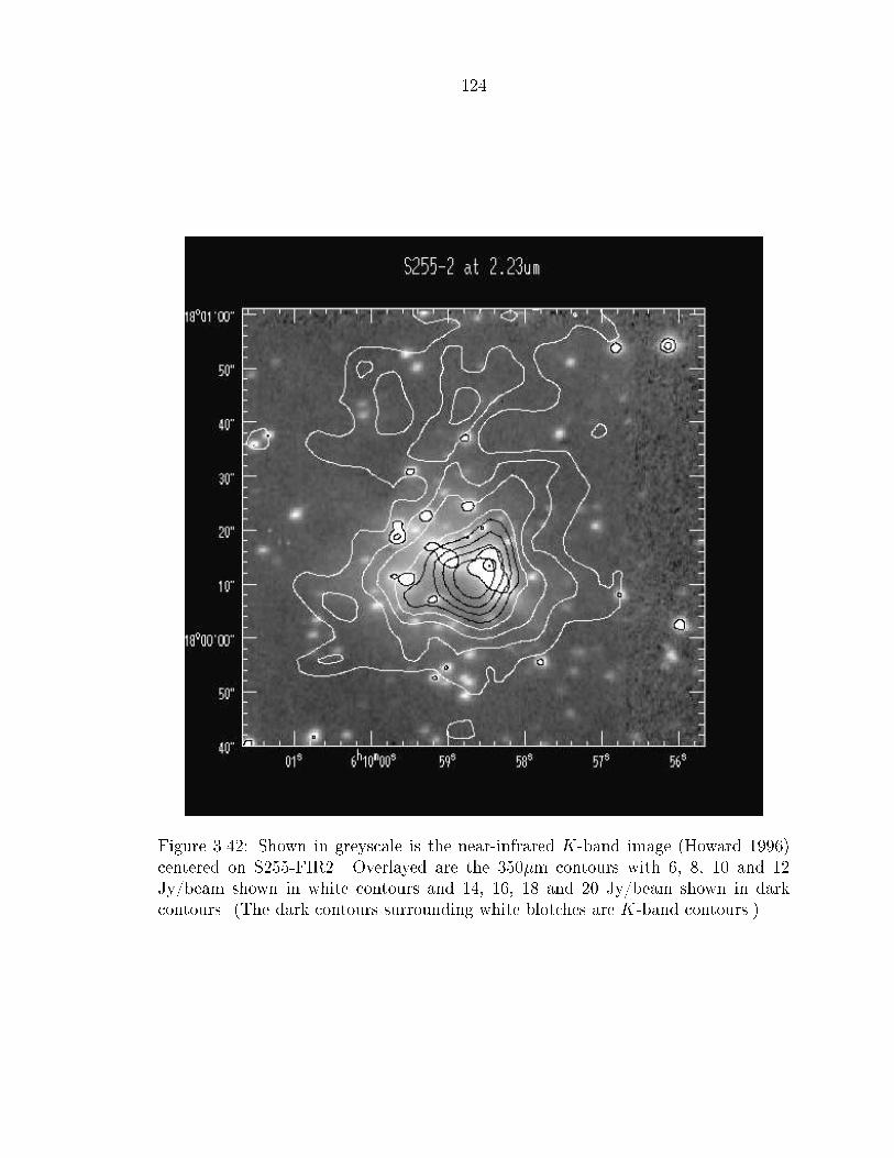
124

Figure 3.42: Shown in greyscale is the near-infrared K-band image (Howard 1996)centered on S255-FIR2. Overlayed are the 350�m contours with 6, 8, 10 and 12Jy/beam shown in white contours and 14, 16, 18 and 20 Jy/beam shown in darkcontours. (The dark contours surrounding white blotches are K-band contours.)

1253.8 SHARC image of the G75 Complex (ON 2)At a distance of 5.6 kpc (Wood & Churchwell 1989), the G75 complex contains severalcenters of compact and extended HII emission. As shown in Fig. 3.43, G75.84+0.40is an extended double-peaked core-halo HII region lying several arcminutes to thenorth (Garay et al. 1993).

Figure 3.43: 6 cm VLA radio continuum image of G75.84+0.34 reproduced fromWood & Churchwell (1989).As shown in Fig. 3.44, G75.78+0.34 (ON 2-N) is a cometary UCHII region lyingseveral arcminutes to the south with associated OH maser emission and a group ofH2O maser spots (Cato et al. 1976; Walker et al. 1978; Downes et al. 1979). Densethermal gas has also been seen in the form of NH3 emission (Churchwell, Walmsley& Cesaroni 1990). G75.77+0.34 is a double-peaked HII region (components A andB) located about 10 southwest of G75.78+0.34 (Matthews et al. 1973).

126

Figure 3.44: 6 cm VLA radio continuum image of G75.78+0.34 reproduced fromWood & Churchwell (1989).Both clusters exhibit 800 and 450�m continuum emission (see Figs. 3.45 and 3.46)but G75.84+0.40 is quite di�use, matching its radio morphology. G75.84+0.40 is alsomuch fainter at 450�m relative to G75.78+0.34 suggesting that much of the �ux isfrom free-free emission. Also, G75.84+0.40 was undetected in H2O and NH3 in thesurvey of Churchwell, Walmsley & Cesaroni (1990) con�rming that it is a more evolvedregion with no dense gas nor compact sources. In contrast, the G75.78+0.34 complexcontains several compact sources in the 450�m SHARC image shown in Fig. 3.46.Overlayed on the map are the positions of the UCHII regions, the millimeter CO, SiOand SO2 peaks (Shepherd & Churchwell 1996b; Haschick & Ho 1990). Apparently,G75.78+0.34 contains a string of sources within a ridge of dust while the HII regionsG75.77+0.34A and B are unassociated with prominent dust emission. Two additionalsubmillimeter sources lie to the southwest: G75.76+0.34, recently detected as an H2Omaser (Hofner 1996b), and G75.75+0.34, unknown at other wavelengths. Like thesubmillimeter clumps in Mon R2 and G34.3+0.2, these sources are candidates formassive protostars which should be observed in depth at near-infrared wavelengths.

127

Figure 3.45: 800�m image of the G75 complex (ON 2). Contour levels are 12 to 52 by4 Jy/beam. Triangles mark the positions of the radio continuum sources associatedwith the northern cluster G75.84+0.4 (Megeath et al. 1990; Pipher, Soifer & Krassner1979) and the southern cluster G75.78+0.34 (Matthews et al. 1973).

128

Figure 3.46: 450�m image of the G75 complex (d = 5:6 kpc) with contour levels-10, 10 to 90 by 10 Jy/beam. Plus symbol: G75.78+0.34 UCHII region and H2Omaser cluster (Hofner 1996b); Filled square: CO J=1!0 peak; Open square: SiOJ=2!1 blob; Filled triangle: 115 GHz continuum peak; Open triangle: SO2 blob(Shepherd & Churchwell 1996b); Asterisk: H2O masers (Hofner 1996b); Crosses: HIIregion components of G75.84+0.40 (Pipher, Soifer & Krassner 1979; Garay et al.1993). The letters A and B mark the positions of the two components of the HIIregion G75.77+0.34 (Matthews et al. 1973). Newly-detected submillimeter sourcesG75.76+0.34 and G75.75+0.34 are indicated by arrows. Dashed lines mark the edgeof the map.

1293.9 Greybody models3.9.1 One-component modelsIn a simple �rst-order analysis, greybody functions have been �t to the spectral energydistribution of the 17 regions imaged with SHARC. A greybody function is simply ablackbody function multiplied by the factor (1 � e��� ) which accounts for the �niteoptical depth �� of the dust cloud at all frequencies �. The three free parameters arethe dust temperature, optical depth and grain emissivity index. The source solid angleand distance is input to the program to convert to observed �ux units. Using a gridsearch least-squares �tting routine (Bevington 1969), a single temperature greybodymodel was used to �t the IRAS 60 and 100�m �uxes and the SHARC 350 and/or450�m �uxes. In most cases, 800 and 1300�m �uxes available from CSO observationsor from the literature were also included in the �t. Assuming a spectral index of �0:1from radio wavelengths, an estimate of the free-free emission contribution to the1300�m �ux was subtracted prior to the �t. Plots of the spectral energy distributionand greybody models for the 17 regions are given in Figs. 3.49 through 3.61. Asummary of the model �t parameters is compiled in Table 3.4 and in Fig. 3.47. Thedata marked by crosses in the top 3 panels of Fig. 3.47 correspond to 3 sources whichdo not have �ux measurements at � > 350�m (G138.295+1.555, G139.909+0.197 andG240.31+0.07). The average dust temperature in the remaining 14 regions is 40� 10K. This is 14 degrees cooler than the average (60�m=100�m) color temperature of all126 UCHII regions studied in the HIRES survey (see Table 3.1). Because the model�ts are less a�ected by the excess �ux in the 60�m band contributed by warm dust,the cooler dust temperatures derived here by including the submillimeter data betterportray the condition of the cool dust grains which account for the bulk of the cloudmass.

1303.9.2 Two-component modelsAs can be seen in Figs. 3.49 through 3.64, the single component greybody models donot �t the observed 12 and 25�m �uxes. Emission at these wavelengths must comefrom warm dust with either low optical depth or small solid angle, i.e., primarily scat-tered light. In the former case, the warm dust could lie in a di�use component moreextended than the submillimeter chopper throw which would not a�ect the submil-limeter �ux measurements. However, if the warm dust is compact, escaping at onlycertain geometries from the core, then it could potentially a�ect the submillimetermeasurements. The HIRES IRAS maps generally show the emission to be compact atthese wavelengths. Therefore, to check whether emission from this warmer componentof dust a�ects the submillimeter portion of the spectrum, two-component greybodymodels were also constructed. Five free parameters were used: the temperature, emis-sivity index and optical depth of the cold dust, and the temperature and optical depthof the warm dust. Because the warm dust probably consists of smaller grains withoutice mantles, the emissivity index of the warm dust was held constant at � = 2. InFigs. 3.49 through 3.61, the two-component models are overlayed in dashed lines withthe one-component models for the 14 sources with �ux measurements at more than5 frequencies. In nearly every source, the two-component model is indistinguishablefrom the one-component model at submillimeter wavelengths. Thus, the warm dustdoes not a�ect the dust properties derived from the one-component models. A com-parison of the temperatures, grain emissivities and optical depths derived from theone and two-component models is given in Table 3.5.3.9.3 Grain emissivity resultsFrom the one-component greybody models, the average grain emissivity index (�) inthe 14 regions with complete submillimeter data is 2:00� 0:25 with a total range of1.35 to 2.30. These results are very consistent with those from a previous study of12 star formation regions where � = 2:0 � 0:4 (Chini, Krügel & Kreysa 1986). Asshown in the top right panel of Fig. 3.47, there appears to be a correlation between

131the emissivity index and the dust temperature with a best �t line of � = (2:89 �0:30)� (0:023� 0:007)T . Because the errors are signi�cant on both axes, the properlinear regression between two random variables was performed (Trinchieri, Fabbiano& Bandiera 1990). The data from a survey of warm clouds with larger HII regions areincluded as open squares in panel 3 of Fig. 3.47 (Gordon 1988). Adding these data, thecorrelation �attens slightly to � = (2:63�0:10)�(0:015�0:002)T . Because it includesdata from 3 warmer clouds in OMC-1, this function is probably more indicative of theunderlying trend of interstellar dust. One explanation for this correlation is that thedust grains in the cooler clouds are more likely to have ice mantles which steepen thegrain emissivity index above � = 2. At the same time, warmer clouds have smallergrains which could �atten the grain emissivity index toward � = 1. However, thecorrelation may simply re�ect the fact that warmer sources exhibit a broader rangeof dust temperatures such that their spectral energy distributions become broadervia a sum of several Planck functions. Single temperature greybody models will thenunderestimate � in order to simulate a broader Planck function (Lis, Carlstrom &Keene 1991).Finally, one of the de�nitions of a Class 0 protostar (Bachiller 1996; Barsony 1995;André 1993) is that it exhibits the ratio Lsubmm=Lbol > 5 � 10�3, where Lsubmm isthe luminosity measured at � > 350�m, or equivalently, log(Lsubmm=Lbol) > �2:30.The average ratio over the 14 UCHII regions is -2.44, only slightly lower than theClass 0 criterion. Evidently, UCHII regions are the high mass equivalent to younglow mass protostars, at least in their appearance at submillimeter wavelengths. Thisagreement simply re�ects the fact that both classes of objects lie deeply embedded inmolecular clouds.

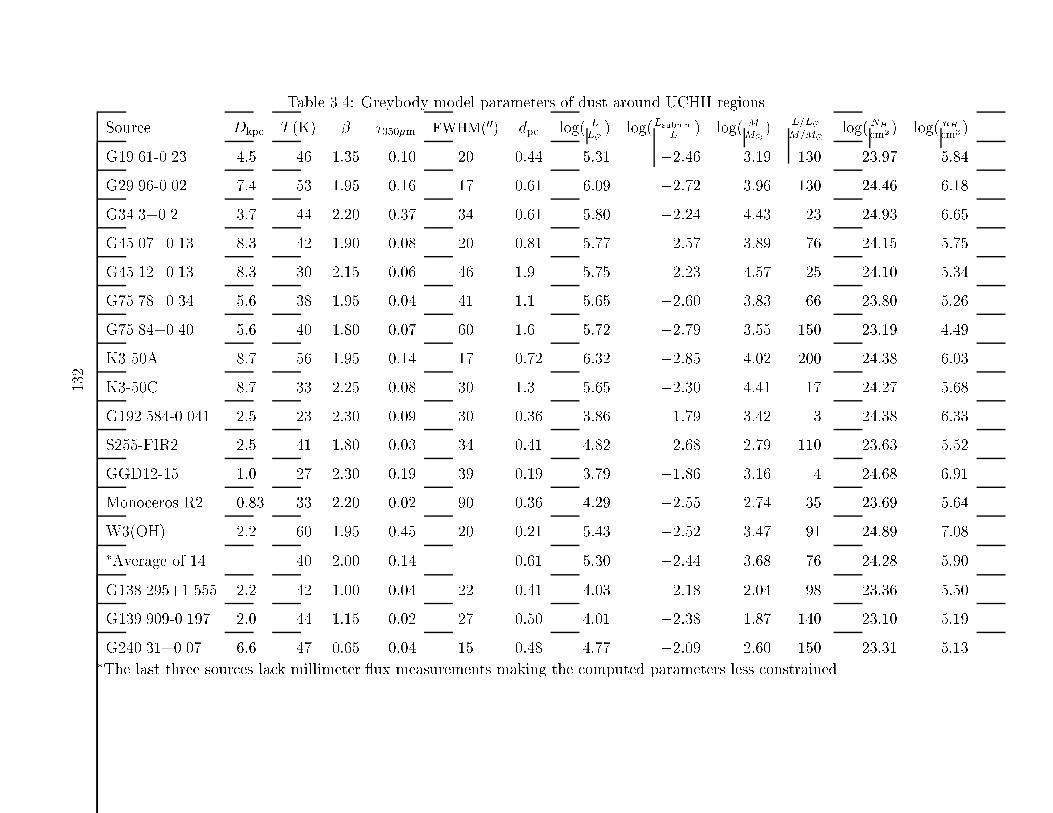
132

Table 3.4: Greybody model parameters of dust around UCHII regionsSource Dkpc T (K) � �350�m FWHM(00) dpc log( LL� ) log(LsubmmL ) log( MM� ) L=L�M=M� log(NHcm2 ) log( nHcm3 )G19.61-0.23 4:5 46 1:35 0:10 20 0:44 5:31 �2:46 3:19 130 23:97 5:84G29.96-0.02 7:4 53 1:95 0:16 17 0:61 6:09 �2:72 3:96 130 24:46 6:18G34.3+0.2 3:7 44 2:20 0:37 34 0:61 5:80 �2:24 4:43 23 24:93 6:65G45.07+0.13 8:3 42 1:90 0:08 20 0:81 5:77 �2:57 3:89 76 24:15 5:75G45.12+0.13 8:3 30 2:15 0:06 46 1:9 5:75 �2:23 4:57 25 24:10 5:34G75.78+0.34 5:6 38 1:95 0:04 41 1:1 5:65 �2:60 3:83 66 23:80 5:26G75.84+0.40 5:6 40 1:80 0:07 60 1:6 5:72 �2:79 3:55 150 23:19 4:49K3-50A 8:7 56 1:95 0:14 17 0:72 6:32 �2:85 4:02 200 24:38 6:03K3-50C 8:7 33 2:25 0:08 30 1:3 5:65 �2:30 4:41 17 24:27 5:68G192.584-0.041 2:5 23 2:30 0:09 30 0:36 3:86 �1:79 3:42 3 24:38 6:33S255-FIR2 2:5 41 1:80 0:03 34 0:41 4:82 �2:68 2:79 110 23:63 5:52GGD12-15 1:0 27 2:30 0:19 39 0:19 3:79 �1:86 3:16 4 24:68 6:91Monoceros R2 0:83 33 2:20 0:02 90 0:36 4:29 �2:55 2:74 35 23:69 5:64W3(OH) 2:2 60 1:95 0:45 20 0:21 5:43 �2:52 3:47 91 24:89 7:08�Average of 14 40 2:00 0:14 0:61 5:30 �2:44 3:68 76 24:28 5:90G138.295+1.555 2:2 42 1:00 0:04 22 0:41 4:03 �2:18 2:04 98 23:36 5:50G139.909-0.197 2:0 44 1:15 0:02 27 0:50 4:01 �2:38 1:87 140 23:10 5:19G240.31+0.07 6:6 47 0:65 0:04 15 0:48 4:77 �2:09 2:60 150 23:31 5:13�The last three sources lack millimeter �ux measurements making the computed parameters less constrained.

133

Figure 3.47: Histograms of the temperature, submillimeter grain emissivity, columndensity, diameter, number density, luminosity, mass and luminosity-to-mass ratioderived from greybody models of the spectral energy distribution of the 17 regionsstudied. 3 regions with non-existent long wavelength (1.3 mm) �ux measurementsare marked by crosses in the top 3 panels. Open squares in the top right panel aredata from Gordon (1988). The vertical dashed line in each panel marks the averagevalue of the 14 sources with complete submillimeter �ux data.

134Table 3.5: Comparison of the one- and two-component greybody modelsOne component Two componentsSource T (K) � �125�m TCold(K) �Cold �Cold:125�m THot(K) �Hot �Hot:125�mG19.61-0.23 46 1.35 0.40 45 1.37 0.46 110 2 1:4� 10�4G29.96-0.02 53 1.95 1.22 49 1.92 1.40 111 2 8:2� 10�4G34.3+0.2 44 2.20 3.63 42 2.25 4.28 110 2 1:5� 10�4G45.07+0.13 42 1.90 0.60 42 1.84 0.53 107 2 2:2� 10�4G45.12+0.13 30 2.15 0.54 38 1.70 0.17 116 2 8:0� 10�5G75.78+0.34 38 1.95 0.27 38 1.92 0.25 114 2 3:6� 10�5G75.84+0.40 40 1.80 0.10 22 3.32 1.84 54 2 1:4� 10�2K3-50A 56 1.95 1.02 55 1.97 1.06 122 2 4:9� 10�4K3-50C 33 2.25 0.80 29 2.75 2.03 60 2 4:3� 10�3G192.584-0.041 23 2.30 1.02 21 2.40 1.36 43 2 1:1� 10�2S255-FIR2 41 1.80 0.18 39 1.84 0.20 132 2 2:2� 10�5GGD12-15 27 2.30 2.03 26 2.07 1.520 58 2 7:1� 10�3Monoceros R2 33 2.20 0.21 33 2.19 0.20 107 2 9:3� 10�5W3(OH) 60 1.95 3.35 47 1.94 2.51 56 2 1.5

135

Figure 3.48: Spectral energy distribution of G19.61-0.23 with the one-component(solid line) and the two-component (dashed line) greybody models overlayed. Listedparameters correspond to the one-component model.

136

Figure 3.49: Same as Fig. 3.48 for W3(OH)

Figure 3.50: Same as Fig. 3.49 for G29.96-0.02.

137

Figure 3.51: Same as Fig. 3.49 for G34.3+0.2.

Figure 3.52: Same as Fig. 3.49 for K3-50 component A.

138

Figure 3.53: Same as Fig. 3.49 for K3-50 component C.

Figure 3.54: Same as Fig. 3.49 for the Monoceros R2 complex.

139

Figure 3.55: Same as Fig. 3.49 for the GGD12-15 complex

Figure 3.56: Same as Fig. 3.49 for G192.584-0.041.

140

Figure 3.57: Same as Fig. 3.49 for S255-FIR2.

Figure 3.58: Same as Fig. 3.49 for G45.07+0.13.

141

Figure 3.59: Same as Fig. 3.49 for G45.12+0.13.

Figure 3.60: Same as Fig. 3.49 for G75.78+0.34.

142

Figure 3.61: Same as Fig. 3.49 for G75.84+0.40.

Figure 3.62: Spectral energy distribution of G139.909+0.197. With only 5 �ux mea-surements, a two-component greybody �t was not possible.

143

Figure 3.63: Spectral energy distribution of G138.295+1.555. With only 5 �ux mea-surements, a two-component greybody �t was not possible.

Figure 3.64: Spectral energy distribution of G240.31+0.07. The �ux measurementsat 20, 27 and 40�m reported by Gezari et al. (1993) are from the AFGL survey.

1443.10 Density pro�les3.10.1 Signature of collapseNumerical analysis of the gravitational collapse of an initially-uniform density, spher-ical gas cloud reveals that the cloud quickly acquires a density pro�len(r) / r�2 (3.19)which resembles an isothermal sphere (Bodenheimer & Sweigart 1968; Larson 1969;Penston 1971; Hunter 1977). This pro�le allows the cloud to approach hydrostaticequilibrium between the outward force of gas pressure and the inward force of self-gravitation. However, there exists an upper limit to the cloud mass above whichequilibrium is impossible in the presence of external pressure from the interstellarmedium (Bonnor 1956), Mcrit = 1:18c4s(G3Pext)�1=2; (3.20)where the sound speed cs is given bycs �s kTmH2 = 0:35 km s�1 for 30 K gas; (3.21)and the external pressure of neutral interstellar gas is given byPext = nkT = 4� 10�12 dyn cm�2 for gas with n = 103 cm�3: (3.22)With these particular parameters, Mcrit = 25M�. If the mass exceeds this criticalvalue, dynamical collapse will follow, proceeding most rapidly in the central regionswhere the density is largest and the free-fall timescale is shortest (Mestel 1965):�free�fall �r 3�32G� / r: (3.23)

145In the outer parts of the cloud, the sound travel timescale is less than the gravitationaltimescale and subsonic motions can produce pressure gradients that oppose and slowthe free-fall. For example, in an isothermal cloud of mass M0 = 10000M� and radiusr0=1.0 pc, (�n = 105 cm�3), the initial gravitational acceleration at large radius isa = GM(< r)r2 � GM0r20 = 0:44� 10�4 km s�1 yr�1: (3.24)Thus, subsonic motions can redistribute material within the outer radii of the cloudfor at least � 104 yr and thereby slow the collapse before the gravitational velocityapproaches the sound speed. Because the cloud is already centrally concentrated,M(< r) = Z r0 �(r0)4�r02dr0 / r; (3.25)a / r�1; (3.26)and hence the gravitational collapse acts more quickly on the inner parts of thecloud, leading to an inside-out collapse. This simple prediction is vindicated by moredetailed solutions to the self-gravitating isothermal �ow problem. In particular, Shu(1977) showed analytically and numerically that in the course of self-similar dynamicalcollapse, the r�2 density pro�le breaks down at small r such thatn(r) / r�3=2; (3.27)and the infall velocity is given by v(r) / r�1=2: (3.28)This con�guration is consistent with a steady mass accretion rate onto the core:_M(r) = 4�r2n(r)v(r) / r0: (3.29)

146Some observational results match these collapse predictions. The earliest measure-ments of the density pro�le of molecular cores were determined from extensive maps oftwo H2CO transitions. Focusing on the nearby low-mass star-forming clouds � Oph A& B and R CrA to get the best spatial resolution, Loren, Sandqvist & Wootten (1983)found that the maps were consistent with radiative transfer models in which thedensity pro�les ranged from r�2 to r�3=2. More recently, radio and millimeter spec-troscopy has been used to search for kinematic evidence for collapse. For example, red-shifted NH3 absorption has been reported toward the UCHII regions W3(OH) (Keto1987; Reid, Myers & Bieging 1987), G34.3+0.2 (Keto 1987), and G10.6-0.4 wherethe infall velocity scales as v / r�0:2 (Keto 1990; Ho & Haschick 1986). Similarly,redshifted HCO+ absorption and blueshifted emission from W51IRS2 and W51e2 areconsistent with large-scale dynamical collapse (Rudolph et al. 1990). By modelingline pro�les, Zhou & Evans (1994) show that infall will create an asymmetry betweenthe strength of the blueshifted and redshifted emission as a function of the opticaldepth of the molecular transition. This e�ect has been observed toward B335 andIRAS16293-2422. Similar results have also been found in the dark clouds (Lynds1962) L1527 and L483 (Myers, Bachiller & Caselli 1995).In addition to spectroscopy, continuum observations of dust provide evidence forcollapsing structures. For example, the 50 and 100�m continuum pro�le of the massivestar-forming region Cepheus A is consistent with the r�3=2 density pro�le (Colomé &Harvey 1995). An IRAS study of 12 Bok globules yielded density pro�les in the rangefrom r�1 to r�5=2 (Yun & Clemens 1991). In a higher resolution study, the millimeterand submillimeter dust emission pro�le from the Bok globule B335 was consistentwith an r�3=2 density pro�le (Chandler, Carlstrom & Terebey 1994). Similar resultsare found in L1527 (Motte, André & Neri 1996), L1489 and L1587 (Ladd et al. 1991)and in L1551IRS5 (Butner et al. 1991). In L1689B, the density pro�le approachesr�2 in the outer regions of the cloud and becomes at least as �at as r�1:2 within0.02 pc (André, Ward-Thompson & Motte 1996). 100�m observations of NGC2071match an r�1 density pro�le (Evans 1989). Observations of the low-mass protostellarsource VLA1623 in the � Oph A cloud indicate an even shallower density pro�le of

147r�1=2 (Barsony 1995). Clearly, further high-resolution observations of dust continuumemission from a larger sample of sources are needed to measure how common eachtype of density pro�le is.3.10.2 The case of massive starsCurrent evolutionary models of massive stars (M > 8M�) predict that hydrogenburning begins before protostellar accretion has ended, precluding a pre-main se-quence phase (Palla & Stahler 1993; Beech & Mitalas 1994). Thus, it is likely thatthe protostellar cloud is still collapsing on a large scale even after the appearanceof the �rst stars (Larson 1972). In attempts to model the dust distribution aroundUCHII regions, Churchwell, Wol�re & Wood (1990) found that constant or very shal-low density pro�les (r�1=2) provide the best �t to the near-infrared to 100�m spectralenergy distributions of these objects. However, emission at these wavelengths is mostsensitive to warm dust near the central star which accounts for a small fraction of thetotal dust mass. By spatially resolving the dust clouds, the maps presented in thischapter allow a more direct measure of the density pro�le. In the following subsec-tions, I model the density pro�le of the dust clouds surrounding the UCHII regions viaradiative transfer simulations in an attempt to match the observed dust continuum�ux pro�le from the submillimeter maps.3.10.3 Flux density pro�les of UCHII regionsAlthough the greybody models characterize the global properties of the dust, they donot immediately indicate the distribution. As seen in Table 3.4, the 350�m opticaldepth of the dust cores is typically much smaller than 1. This means that the �uxdensity in a given aperture is proportional to the temperature-weighted mass in thebeam. Because the dust emission is resolved in many of the SHARC images, there ismore information to be gleaned. Aperture photometry was performed on each of theUCHII regions, recording the �ux density in apertures of logarithmically increasingradii about the centroid of the source. The average �ux density per pixel in the

148outermost ring inscribed in the map was subtracted as a background value from allpixels in the inner apertures; but typically there was no signi�cant o�set present.3.10.4 Radiative transfer modelsOne can compare the submillimeter �ux density pro�le to predicted pro�les fromradiative transfer models. (To avoid confusion with the particle density pro�les, �uxdensity pro�les are hereafter referred to as ��ux pro�les.�) For this purpose, I havemodeled the appearance of dust cocoons around UCHII regions with the radiativetransfer program CSDUST which solves for the dust temperature at all radii withinthe cocoon (Egan, Leung & Spagna 1988).3.10.4.1 Input parametersEven with the assumption of spherical symmetry, a complete model requires manyinput parameters: the dust emissivity index (�), the normalized mass opacity of thedust (�0) at some speci�ed frequency �0, an initial dust temperature distribution(T (r)) the outer boundary of the cloud (ro), the inner core radius of the cloud wherethe power-law density pro�le levels o� (ri), the power-law index of density pro�le (p),the optical depth at �0 from the center to the surface, the luminosity Lbol and e�ectivetemperature Te� of the internal heat source, and the external radiation �eld intensity.In the following simulations, �, �120�m, and Lbol are taken from the greybody modelsfor each source and a normalized dust emissivity of 7:5� 10�4 at 120�m is assumed(Hildebrand 1983). At wavelengths shorter than 100�m the dust emissivity index isset to 1.0 to match the typical observed values in the mid-infrared (Hildebrand 1983):Q� = Q125�m�125�m� ��; for � > 100�m; (3.30)= Q125�m�125�m100�m���125�m� �1:0; for � � 100�m; (3.31)where Q125�m = 7:5� 10�4: (3.32)

149A �nal constraint is placed such that Q� � 1:0 at short wavelengths. Te� is takenfrom the zero age main sequence values for a star with the appropriate value of Lbol(Thompson 1984; Panagia 1973). An external radiation �eld of one standard ISRF isalso assumed.3.10.4.2 Model procedureBecause of sensitivity limitations in the maps, especially to emission structures largerthan the chopper throw, the true outer boundary of the cloud ro is uncertain andshould be varied to obtain the most accurate model (e.g., Mundy et al. 1996). How-ever, as a simpli�cation to the model procedure owing to time constraints on thisresearch, the value of ro has been �xed at the radius where the intensity of the sub-millimeter emission vanishes (usually equal to or close to the size of the map). Modelswere then run for 3 di�erent power-law density pro�le indices, p = 1; 1:5, and 2. Theresults are compared to the observations and the value of p most consistent with thedata is assigned to the source. As a self-consistency check, the predicted spectralenergy distributions of the 3 models are compared to the measured FIR and sub-millimeter �ux densities to con�rm that the assigned value of p provides the best�t. Regarding the starting point for T (r), radiative transfer models of infrared sourcesin molecular clouds have previously revealed that T (r) / r�q (Goldreich & Kwan1974; Scoville & Kwan 1976) where q = 2=(4 + �) (Harvey et al. 1991; Adams 1991).Thus the input temperature distribution was computed for each source using thevalue of � from the greybody model and normalizing the temperature at the half-power radius to the greybody temperature. The program CSDUST modi�es thisdistribution slightly after each iteration while converging toward equilibrium. Becausepower-law density pro�les become singular at the origin, it is necessary to cap them atsmall radii. The program achieves this requirement by smoothly matching the inputpower-law density pro�le to a Gaussian density pro�le. The match point (ri) is setto the radius inside of which 80% of the optical depth lies. Typically this occurs at afractional radius of 0.05. Repeated models with the match point set to 90% revealed

150that the model �ux pro�les are fairly insensitive to the match point over the range offractional radii probed by the observations.3.10.5 Convolution with the instrumental beam patternOnce the radiative transfer model has converged, the result must be convolved withthe telescope beam to obtain a prediction of the observed �ux pro�le at a speci�cwavelength. To do this properly, I have modeled the instrumental beam responseto a point source from images of Uranus. Because its angular diameter (� 3:005) ismuch smaller than the beamsize, it can be taken as a good approximation to a pointsource. Shown in Fig. 3.65 is the integrated �ux pro�le extracted from the 350�mimage of Uranus obtained with a chopper throw of 8700 (Fig. 3.66). Overlayed on theobservations is the �ux density pro�le of a 1400 Gaussian beam which matches the full-width half-power diameter in the Uranus image but fails to match the broad wingsof the response. As discussed in Chapter 2, the SHARC/CSO beam response can bedescribed by a sum of two functions: a di�raction-limited component (convolved withthe pixel size) and a larger sidelobe component. In Fig. 3.65 I have also overlayed the�ux pro�le predicted by the sum of two Gaussian beams: a 1200 beam with 75% of thepower and a 3000 beam with 25% of the power. Although the main beam e�ciency ofthe CSO is known to be only � 30% at 350�m, much of the sidelobe power evidentlylies in an even more extended error pattern which is either chopped out or too faintto be seen in the beam map. Thus, the emergent intensity at each impact parameterof the radiative transfer model has been convolved with the sum of these two beamsin order to derive the predicted �ux pro�le.In Figs. 3.67 through 3.79, I compare the observed �ux pro�le with predicted �uxpro�les from the CSDUST radiative transfer models with particle density pro�les ofn(r) / r�2, n(r) / r�3=2 and in some cases n(r) / r�1. Mon R2 is excluded from thisanalysis as it is clearly a non-spherical cluster of individual sources (primarily becauseit is the nearest source in the survey). The rest of the sources can be characterizedinto four categories: isothermal, central collapse, bulk collapse, and logatropic.

151

Figure 3.65: Observed �ux pro�le of Uranus measured from the 350�m image andcompared to predictions from a 1400 Gaussian beam which matches the half-powerdiameter, and the sum of a 1200 Gaussian main beam and a 3000 Gaussian sidelobebeam which provide a better match to the response pattern.

152

Figure 3.66: 350�m SHARC image of Uranus in celestial coordinates from which the�ux pro�le of Fig. 3.65 was measured. Contour levels are 2.5%, 5%, 10% to 90% by10%. The dashed contours represent the half-power levels of the 1200 and 3000 Gaussianbeams that comprise the model of the response pattern.

1533.10.6 Sources resembling an isothermal sphereAt all scales, the �ux pro�le of G240.31+0.07 closely matches the n / r�2 densitypro�le of the isothermal sphere, suggesting that it is in an early stage of star formationdevelopment before substantial collapse has occurred. As discussed in section 3.7.1,so far there is evidence for only a single object forming in this core.

Figure 3.67: Observed �ux pro�le of G240.31+0.07 measured from the 350�m imageand compared to predictions of radiative transfer models.

154Like G240.31+0.07, G19.61-0.23 resembles the isothermal sphere throughout mostof the cloud, although the slope appears to become shallower in the outermost regions.This broadening may be due to fainter subclumps in the halo, especially since a clusterof 5 UCHII regions is seen in this source (see Fig. 3.25 in Section 3.5.3).

Figure 3.68: Observed �ux pro�le of G19.61-0.23 measured from the 450�m imageand compared to predictions of radiative transfer models.

155The �ux pro�le of G29.96-0.02 matches the isothermal sphere through most ofthe cloud though it appears to deviate slightly in the inner regions. However, smallpointing and tracking errors between subsequent scans of the map may broaden thepro�le up to � 200. This e�ect will be especially noticeable at small radii. Thus withinthe estimated error, the observed pro�le is consistent with the isothermal sphere atall scales. The presence of the UCHII region, a separate concentration of H2O masers,and a small near-infrared cluster indicates several sites of star formation already existat the core.

Figure 3.69: Observed �ux pro�le of G29.96-0.02 measured from the 450�m imageand compared to predictions of radiative transfer models.

1563.10.7 Sources resembling the collapse pro�le at the centerThe �ux pro�le of W3(OH) matches the isothermal sphere in the outer parts of thecloud but rapidly approaches the n(r) / r�3=2 law at the innermost radii. This pro�leis consistent with collapse in the central core (r . 1000 or 0.1 pc), while the outerregions (r & 4000 or 0.4 pc) remain isothermal and have not yet felt the collapse. Toestimate the time since the collapse began, I assume uniform gravitational accelerationand set the collapse velocity at r = 0:4 pc equal to the sound speed (Eq. 3.24). Usingthe mass and temperature from Table 3.4, this yields a timescale of 5�103 yr, virtuallyidentical to the typical dynamical timescale of UCHII regions derived in Chapter 1.Note that there are at least two young objects already formed in this core: the UCHIIregion and the Turner-Welch object.

Figure 3.70: Observed �ux pro�le of W3(OH) measured from the 350�m image andcompared to predictions of radiative transfer models.

157Like W3(OH), the �ux pro�le of K3-50A matches the prediction of the isothermaldensity pro�le in the outer regions of the cloud and approaches the collapse pro�lein the inner regions. Like W3(OH) there is evidence for several young objects in thiscore, the UCHII region, an out�ow source lying to the east (identi�ed in Chapter 4)and a possible near-infrared cluster (Howard et al. 1996).

Figure 3.71: Observed �ux pro�le of K3-50A measured from the 350�m image andcompared to predictions of radiative transfer models.

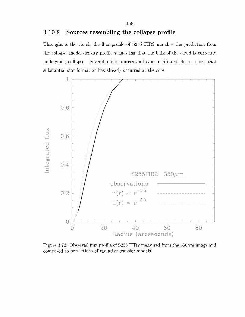
1583.10.8 Sources resembling the collapse pro�leThroughout the cloud, the �ux pro�le of S255 FIR2 matches the prediction fromthe collapse model density pro�le suggesting that the bulk of the cloud is currentlyundergoing collapse. Several radio sources and a near-infrared cluster show thatsubstantial star formation has already occurred at the core.

Figure 3.72: Observed �ux pro�le of S255 FIR2 measured from the 350�m image andcompared to predictions of radiative transfer models.

159On all scales, the �ux pro�le of G75.78+0.34 lies between the predictions fromthe isothermal and collapse model density pro�les. It appears to be consistent with apro�le of r�1:75; however, the models are not easily distinguishable due to the limitedspatial resolution achieved on this source. Nevertheless, it will be classi�ed here asa collapse pro�le. Like W3(OH) and K3-50A, there is evidence for more than oneyoung object forming in this core (Shepherd & Churchwell 1996b).

Figure 3.73: Observed �ux pro�le of G75.78+0.34 measured from the 450�m imageand compared to predictions of radiative transfer models.

160In the outer half of the cloud, the �ux pro�le of G45.07+0.13 matches the pre-diction from the collapse model density pro�le suggesting that the entire cloud iscurrently undergoing collapse. As in G29.96-0.02, the slight broadening of the pro-�le at small radii is consistent with a 200 tracking error. To date, only the UCHIIregion/H2O maser source has been identi�ed in this distant source.

Figure 3.74: Observed �ux pro�le of G45.07+0.13 measured from the 350�m imageand compared to predictions of radiative transfer models.

161Based on the image in Fig. 3.17, the outer parts of the �ux pro�le of G34.3+0.2is obviously widened due to contamination from of additional point sources in theextended halo. Without this confusion, the pro�le would likely exhibit the collapsepro�le throughout the cloud, as it does in the inner regions. The UCHII region, H2Omaser sites, and submillimeter sources reveal multiple cores of star formation in thiscloud.

Figure 3.75: Observed �ux pro�le of G34.3+0.2 measured from the 450�m image andcompared to predictions of radiative transfer models.

1623.10.9 Sources resembling logatropic spheresThe pro�le of K3-50C, a ridge-like source containing 3 UCHII regions, is consistentwith a shallower density pro�le of n(r) / r�1. This type of pro�le is known as alogatropic sphere (Lizano & Shu 1989) and implies equal column density on all scales.The structural analysis of dark clouds by automatic starcounts yields an internaldensity structure of n(r) / r�1:0�0:4 (Stüwe 1990), and in particular for the Taurus-Auriga complex, n(r) / r�1:3 (Cernicharo, Bachiller & Duvert 1985). Similarly, thedistribution of the average densities of molecular clouds of varying radius follows therelation n / r�1:1 (Larson 1981). Therefore, this density pro�le may be the signatureof either a cluster of dust cores (consistent with the 3 UCHII regions found here).

Figure 3.76: Observed �ux pro�le of K3-50C measured from the 350�m image andcompared to predictions of radiative transfer models.

163The pro�le of G45.12+0.13 exhibits a similar shallow pro�le to that seen in K3-50C. Including the UCHII region, this source contains at least 2 young objects without�ows (see Chapter 5).

Figure 3.77: Observed �ux pro�le of G45.12+0.13 measured from the 450�m imageand compared to predictions of radiative transfer models.

164Like G45.12+0.13 and K3-50C, GGD12-15 matches the n(r) / r�1 power-law. Atleast two sources, the UCHII region and H2O maser, have formed in this relativelylower luminosity object (L < 104L�).

Figure 3.78: Observed �ux pro�le of GGD12-15 measured from the 350�m image andcompared to predictions of radiative transfer models.

165G192.584-0.041 also matches the n(r) / r�1 law throughout the cloud. Althoughonly a single dominant radio source has been detected, there is an infrared cluster aswell as faint radio and submillimeter emission to the north. Like GGD12-15, it is oneof the lowest luminosity sources in the sample.

Figure 3.79: Observed �ux pro�le of G192.584-0.041 measured from the 350�m imageand compared to predictions of radiative transfer models.

166G138.295+1.555 also matches the n(r) / r�1 law throughout the cloud. As dis-cussed in section 3.7.2, this cloud contains two radio sources and an infrared clusterof at least 30 stars. Like GGD12-15 and G192.584-0.041, it is one of the lowestluminosity sources in the sample.

Figure 3.80: Observed �ux pro�le of G138.295+1.555measured from the 350�m imageand compared to predictions of radiative transfer models.

167Finally, G139.909-0.197 also matches the n(r) / r�1 law. Like G138.295+1.555,this lower luminosity cloud contains more than two dozen young stars and possiblyas many as �ve dozen (Weintraub & Kastner 1996; Weintraub et al. 1996).

Figure 3.81: Observed �ux pro�le of G139.909-0.197 measured from the 350�m imageand compared to predictions of radiative transfer models.

1683.10.10 Con�rmation of the spectral energy distributionsBesides predicting the �ux pro�les discussed in the preceding section, the radiativetransfer models also predict the total source �ux as a function of wavelength. Fora self-consistency check, these predictions can be compared to the measured �uxesthat were used to �t the greybody models in section 3.9. Plotted in Fig. 3.82 arethe predicted spectral energy distributions (SEDs) from the radiative transfer modelfor each source. Separate curves are plotted for the r�2, r�3=2 and the r�1 densitypro�les. In nearly every case, the measured far-infrared and submillimeter �uxes lie(within the error bars) on the appropriate curve that matches the �ux pro�le. Likethe one-component greybody models, the curves tend not to match well with the mid-infrared (12 and 25�m) �uxes. Apparently the dust model is not detailed enough totreat these wavelengths properly. Since only a single dust grain size was used, thisshortcoming is not surprising. A more complex model would be necessary to treatfeatures such as the mid-infrared silicate bands. However the simple model presentedhere does serve well at the wavelengths of interest.3.10.11 Temperature distributionsPlotted in Fig. 3.83 are the equilibrium temperature distributions from the radiativetransfer models. As can be seen by the thin straight lines overlayed, the simple scalinglaws of T (r) / r�2=5 or r�1=3 (corresponding to � = 1 or 2) are good approximationsto the model temperature distributions in the outer parts of the cloud. The generalupturn in the model temperature occurs about the radius at which the model power-law density pro�le is matched to a Gaussian pro�le.

169

Figure 3.82: The predicted spectral energy distributions from the radiative transfermodels are plotted as curves; dotted: � / r�2, dashed: r�3=2, dash-dot: r�1. The boxesmark the observed �uxes from each source corresponding to IRAS, submillimeter, andmillimeter measurements.

170

Figure 3.83: The predicted temperature distributions from the radiative transfermodels are plotted as curves; dotted: � / r�2, dashed: r�3=2, dash-dot: r�1. Thestraight lines mark the simple scaling laws of T (r) / r�1=2; r�2=5 and r�1=3 (from topto bottom). The upturns in the model temperature at small radii correspond to thecore radius where the power-law density pro�le is matched to a Gaussian pro�le.

1713.11 Luminosity to mass ratiosWith the density pro�le analysis complete, a �nal relation to explore in these UCHIIregions is their FIR luminosity to dust mass ratio (LFIR=Mdust) versus dust tempera-ture. As evident in Table 3.4, a large range exists in the LFIR=Mdust ratio (3 to 200).Because the FIR dust emission derives from re-processed starlight originating at thecore of molecular clouds, the LFIR=MCO ratio has been quoted as a measure of thestar formation rate of whole galaxies and individual giant molecular clouds (Young etal. 1986; Mooney & Solomon 1988; Scoville & Good 1989; Carpenter, Snell & Schlo-erb 1990). Typically, the mass has been determined from CO observations; but inthis case, we can measure the dust mass directly from the greybody models. Becausethe FIR dust luminosity is proportional to dust mass and the frequency integral ofthe modi�ed Planck function, the LFIR=Mdust should be proportional to the latterquantity (Cox & Mezger 1989):LFIRMdust / Z 10 B�(Tdust)Q�d� / Z 10 B�(Tdust)��d� / T 4+�dust : (3.33)As expected, Fig. 3.84 indicates a strong correlation between the LFIR=Mdust ratioand the dust temperature of UCHII regions. No correlation is seen in the LFIR versusTdust diagram due to the range of masses present in the source sample. A simpleexplanation for the observed LFIR=Mdust vs. Tdust relation is that it represents anevolutionary track. That is, the more evolved sources lie to the upper right becausethey have formed a greater number of hot stars that have boosted the luminosityand heated the dust to a higher temperature over a longer period. However, thesources tend to group together on the LFIR=Mdust vs. Tdust diagram as a functionof their density pro�le, with isothermal cores showing the largest LFIR=Mdust ratiosand temperatures and logatropic cores showing the smallest. In other words, themore centrally-condensed cores contain warmer dust. A similar correlation is seen inextragalactic studies in which merging and interacting galaxies lie to the upper rightand isolated galaxies lie to the lower left of the LFIR=MCO vs. (F60�m=F100�m) diagram

172

Figure 3.84: Upper panel: The luminosity plotted against the dust temperature fromthe one-component greybody model. Letters denote the UCHII regions whose densitypro�les indicate the isothermal (I), collapse (C), isothermal/collapse (IC) and logat-ropic (L) pro�les. Filled triangles mark the UCHII regions with no long wavelength�ux measurements and open triangles mark Mon R2 and G75.84+0.40 for which den-sity pro�les could not be reliably measured. Squares mark HII regions from Gordon(1988). There is little correlation due to the range of masses in the sample. Lowerpanel: Same as the upper panel for the luminosity to dust mass ratio, a measureof star formation e�ciency which correlates with dust temperature. Overlayed is apower law �t consistent with a modi�ed Stefan-Boltzmann law with � = 0:71.

173(Young 1990). Thus, perhaps the range of values is not established directly by thetime evolution in the star formation rate from lower to higher values of LFIR=Mdust.Instead, a range of initial conditions may determine the collapse density pro�le, whichin turn sets the star formation rate and the dust temperature. Speci�cally, cloudswith steeper radial density pro�les yield higher star formation rates and warmer dust.A further argument against simple time evolution is that because all of the sourcescontain UCHII regions, they may all be of similar age and in a similar evolutionarystage.3.12 SummaryThe dust cores surrounding a sample of 17 UCHII regions are resolved for the �rsttime in the high-resolution submillimeter continuum images presented in this chapter.The �rst impression left by the images is the presence of clusters of dust emission.Undoubtedly the UCHII regions dominate the peak emission due to the warm dustsurrounding them. However, in many cases, cores of lower level emission lie in theirvicinity. H2O masers are often found in these sub-cores, although many are not as-sociated with any known maser or radio continuum source. These newly-identi�edsources should be followed up with deep near-infrared surveys to search for the coun-terparts of these massive, possibly protostellar sources.As a sample, the sources cover a fairly wide range of bolometric luminosity(104 to 106L�) and temperature (23 to 60 K). One-component and two-componentgreybody models show that the submillimeter emission can be characterized accu-rately by a single temperature and grain emissivity index. The average temperatureis 40 � 10 K and the average grain emissivity index (�) is 2:00 � 0:25, consistentwith results from prior 1.3 mm surveys. Using power-law density pro�les of the formn(r) / r�n, radiative transfer models successfully predict the �ux pro�le of thedust. Three of the sources are consistent with r�2 resembling an isothermal cloud.In two sources, the outer parts of the cloud are consistent with the r�2 pro�le whilethe inner parts approach the shallower r�1:5 pro�le indicative of dynamical collapse.

174The appearance of these two sources is likely to be short-lived as the collapse hasbeen occurring for only � 5000 yr. Four sources are consistent with the r�1:5 pro�lethroughout the cloud, possibly indicating a more advanced state of collapse. The �nalsix regions are shown to exhibit a density pro�le approaching the r�1 law, similar tothat seen in nearby extended dark clouds.It should be noted that of the six logatropic sources, four are the least distant(d < 2:5 kpc) regions in the sample. These four are also the lowest luminosity sourcesin the sample (L < 104:3L�) corresponding to stellar types later than B0.5. In mostcases, these regions show evidence for a cluster of young embedded stars on scaleslarger than the beamsize. Hence it is no surprise that they appear more like locallow-mass star-forming dark clouds than the rest of sample. When these four sourcesare discarded from the statistics, over half (6 out of 11) UCHII regions exhibit thecollapse density pro�le to some degree. These results are summarized in Table 3.6.Table 3.6: Summary of dust density pro�lespower-law # sources with % of sources withDensity pro�le index # sources L > 104:3L� L > 104:3L�isothermal r�2 3 3 27%isothermal/collapse r�2=r�3=2 2 2 18% �55%collapse r�3=2 4 4 36%logatropic r�1 6 2 18%Finally, an interesting discovery is that sources with similar density pro�les lie insimilar areas of the LFIR=Mdust (star formation rate) vs. Tdust diagram. Isothermalclouds lie to the upper right where the star formation rate is high, while logatropicclouds lie to the lower left where the rate is low. Apparently, clouds with morehighly concentrated density pro�les develop star formation more rapidly than othercon�gurations. Because all the clouds contain UCHII regions with typical lifetimes of� 5�104 yr, it is possible that this di�erence arises from di�erent physical conditions(such as the relative importance of magnetic �eld support) rather than being di�erentevolutionary states of a general track.As expected from the relative timescales, the inner region and in many cases thebulk of the dust cloud is still collapsing even after the �rst OB star(s) have formed near

175the core. Opposing the collapse motion are bipolar molecular out�ows from youngembedded objects in the core. It has been proposed that out�ows may ultimatelylimit the mass of an accreting star (Silk 1995). Measuring the strength of out�owsfrom these clouds and determining whether the UCHII regions or associated sourcesdrive the out�ows is the subject of the next chapter.

176Chapter 4 Molecular Out�ows from UCHIIRegions4.1 Characteristics of molecular out�owsAt some point during the formation process of a new star, an out�ow phase beginswhich can manifest itself in various observational forms including the bipolar molecu-lar out�ow (Lada 1985; Bachiller & Gómez-González 1992; Bachiller 1996). Molecularout�ows are most commonly observed as high velocity wings in the rotational tran-sitions of CO, the most abundant interstellar molecule after H2. These line wingsusually extend to velocities of 5-30 km s�1 away from the systemic velocity but canreach to velocities > 100 km s�1 in the case of extremely high velocity (EHV) bullets(such as in HH7-11, Lizano et al. 1988; Masson et al. 1990; Bachiller & Cernicharo1990). Although not yet fully understood, the acceleration mechanism of the molec-ular gas must be intimately related to the star formation process (Shu et al. 1994).When the high velocity CO emission can be resolved spatially, it usually exhibits acollimated bipolar morphology, analogous to the ionized jets sometimes seen at visibleand radio wavelengths from young stellar objects (e.g., Reipurth & Heathcote 1993;Staude & Elsässer 1993). In many cases, the CO out�ows align with bright knotsof emission nebulae known as Herbig-Haro (HH) objects which often exhibit largeproper motions implying velocities of � 200 km s�1 away from the driving source (seereferences in Schwartz 1983). The similar morphology of these phenomena suggestsa common driving mechanism and invites a comparison of their physical attributes.4.1.1 Momentum comparison between jets and out�owsAn important physical measure of a jet or out�ow is the force, or the rate at whichmomentum is deposited into the �ow. Usually the force F is expressed as the product

177of the mass loss rate _m and the �ow velocity v. In the case of optical jets, v can bedetermined from high resolution spectroscopy of the H� line. With H� imaging, onecan measure the length of the jet and compute a kinematic age t, the dynamicalcrossing timescale. The electron density ne can be estimated from the intensity ratioof forbidden lines such as the 6717 and 6731 Å lines of ionized sulfur (Hartmann& Raymond 1984). Combining ne with the linear dimensions of the jet leads to anestimate of the mass m of ionized gas in the �ow. Combining these parameters yieldsthe out�ow force: F = _mv = mvt = mvr=v = mv2r : (4.1)In the case of molecular out�ows, v can be determined from CO spectra, r fromthe CO maps, and m from the integrated CO emission (Lada 1985). In the caseof L1551 IRS5, the force observed in the optical jet (Sarcander, Neckel & Elsässer1985) is 2 to 3 orders of magnitude less than the force required to drive the molecularout�ow (Moriarty-Schieven & Snell 1988). This result has been typical of youngstellar objects; the force exerted by the ionized gas of optical jets is about 2 ordersof magnitude too small to drive the molecular out�ows (Mundt, Brugel & Bührke1987). Consequently, it was widely speculated that the two phenomena had separateorigins, with the optical jet being driven by a collimated stellar wind while the largermolecular out�ow was driven by a wide-angle wind from the accretion disk (Pudritz1988; Pudritz & Norman 1983).However, the discrepancy in momenta of jets and out�ows has been eased by thediscovery of two key facts. First, it was realized that the out�ows may be much olderthan previously assumed. The typical kinematic age of molecular out�ows is � 104 yr(Masson & Chernin 1993). However, in a survey of a well-de�ned sample of IRASsources from the Class I or Class II-D phase of low-mass young stellar objects (asde�ned by Adams, Lada & Shu (1987)), 9 out of 12 embedded IRAS point sourcescontained out�ows (Parker, Padman & Scott 1991). The combined duration of theClass I and II-D phases is believed to be 2:5 � 105 yr (Beichman et al. 1986; Myers

178et al. 1987). Therefore, the statistical lifetime � of the out�ows is� = �number of sources with out owsnumber of sources � = � 912�2:5� 105 yr = 1:9� 105 yr:(4.2)A similar lifetime has been derived by comparing the number of out�ow sources withthe number of optically-identi�ed T Tauri stars in the nearby dark cloud L1641 (Fukui1993).Second, calculations suggest that much of the optical jet material (� 98%) isneutral gas (Hartigan, Morse & Raymond 1994; Raga, Binette & Cantó 1990). Thepresence of neutral gas in jets has been con�rmed by the detection high-velocity HIemission in the 21 cm line from HH7-11 (170 km s�1) (Lizano et al. 1988) and L1551(260 km s�1) (Giovanardi et al. 1992). The combination of these two facts can closethe gap in momentum between the two di�erent phenomena (Raga 1991; Padman &Richer 1994). For example, it has been observed that the HH111 jet may providesu�cient momentum to drive the surrounding CO out�ow in L1617 (Cernicharo &Reipurth 1996). Similar results are found in the red nebulous object RNO43 (Bence,Richer & Padman 1996). Finally, the fact that both jets and out�ows are high-velocity and highly-collimated structures points to a common driving and collimationmechanism near the central source (Masson & Chernin 1994). They could well bedi�erent manifestations of the same phenomenon.4.1.2 Conservation of momentum in out�owsOne of the observational constraints on molecular out�ow models is that they appearto be driven by a process that conserves linear momentum. Because out�ows generallyexhibit strong bipolarity in both velocity and space, the transverse velocity of materialmust be small compared to the radial velocity along the axis of the �ow. This featureis a natural characteristic of a momentum-driven �ow. In contrast, a pressure-driven�ow that conserves energy would tend to in�ate bubbles of ambient gas, leading tolarger transverse velocities than are observed (Meyers-Rice & Lada 1991). Such a �ow

179would also exhibit backward moving material in each lobe which is generally not seen.Furthermore, such a �ow cannot be collimated by the ambient cloud without inducingsubstantial transverse motion in the collimating mass (Takano et al. 1984). Thus,out�ows must be driven in a momentum-conserving manner by a bipolar collimatedwind at the central source (Masson & Chernin 1993).4.1.3 Momentum transfer in jet-driven out�owsIn parallel with these new conclusions, uni�ed models of jet-driven molecular out�owshave been developed (Raga et al. 1993; Raga & Cabrit 1993; Masson & Chernin 1993;Chernin et al. 1994). In general, the models must transfer momentum (P ) from asupersonic jet to the dense ambient gas that will comprise the molecular out�ow. Therate of momentum transfer can be written:dPdt = _P = ( _mv)out ow = �( _mv)jet; (4.3)where � is the entrainment e�ciency, which equals 1 if the jet is completely stoppedby the ambient material. The physical device used in the models to accomplish themomentum transfer from the jet to the out�ow is a bow shock. When a supersonic jetimpacts stationary gas, the jet rapidly decelerates in a jet shock while the ambient gasis accelerated by a forward bow shock (Blandford & Rees 1974). Following Cherninet al. (1994), the rate of momentum transfer ( _P ) at the working surface (ws) of a bowshock is: _P = �jetAws(vjet � vws)2 = �BS�jetAjetv2jet; (4.4)where �BS is the entrainment e�ciency of the bow shock, Ajet is the geometrical areaof the jet, AWS is the geometrical area of the working surface of the bow shock, and�jet is the gas density in the jet. One can solve this equation for �BS in terms of the

180observable parameters: �BS = AwsAjet�1� vwsvjet�2: (4.5)In the limit that all of the energy released in the bow shock is immediately radiatedaway, there is no additional thermal pressure and the ram pressure in the jet equalsthe ram pressure of the swept-up medium at the working surface of the bow shock:_mjetvjet = _mambientvws (4.6)�jetAjet(vjet � vws)2 = �ambientAwsv2ws: (4.7)Using the quadratic formula, one can solve for the velocity of the working surface:vws = vjet� p��1 +p��� (4.8)where � � �jet�ambient (4.9)and � � AjetAws : (4.10)In this case, the bow shock entrainment e�ciency then becomes:�BS = 1�� 11 +p���: (4.11)Chernin et al. (1994) have computed three-dimensional smoothed particle hydrody-namic simulations of jets in which the jet area and bow shock areas are equal (� = 1)and with several di�erent values of density contrast (�) and jet Mach number (M).The jet radius was rjet = 2� 1016 cm and the sound speed in the jet was 12 km s�1,appropriate for ionized gas with T � 104 K from Eq. 3.21. These simulations showthat in the case of a high Mach number jet (M = 30, v = 350 km s�1), � � �BS andthe jet is not decelerated signi�cantly until it reaches a radius of � 20rjet, or 0.13 pc(corresponding to 2700 at a distance of 1 kpc). Ambient gas is entrained only at theend of the jet, a process called prompt entrainment (DeYoung 1986). This processleads to a parabolic-shaped nebula with the vertex at the bow shock and the curve

181opening toward the driving source. However, in a low Mach number jet (M = 3,v = 39 km s�1) �BS is a factor of a few smaller than � and the jet is deceleratedby � 25% by the time it �ows a distance = 3rjet. In this case, called steady-state (orturbulent) entrainment, the ambient gas is entrained essentially along the entire jet.Because the transverse motion of gas remains roughly constant, this process createsa conical out�ow of increasing radius with distance.4.1.4 Comparison to observationsThe detection of EHV features in out�ows is the most important piece of evidence forjet-driven out�ows. EHV gas requires that protostellar jets have high Mach numbers,suggesting that prompt entrainment dominates the �ow. This process can explainthe common observational �nding that the highest velocity gas shows the highestdegree of collimation as in the out�ows of NGC2024 FIR5 (Richer, Hills & Padman1992) and NGC2264G (Lada & Fich 1996). A speci�c numerical model of Cherninet al. (1994) with high Mach number and � = � = 1 actually predicts the existenceof a small clump of gas (10�3M�) moving at 100 km s�1 in the post-shock region.In this case, � � �BS = 0:25, implying that the momentum transfer is 25% e�cient.Another observational �nding that may support the bow shock model is the frequentpresence of infrared re�ection nebulae near the origin of molecular out�ows (Hodapp1994; Hunter et al. 1995). Although they may be illuminated by radiation from youngstellar clusters, these nebulae could also be powered in part by the cooling radiationfrom bow shocks (Testi et al. 1994).Even though the jet-driven out�ow model of Chernin et al. (1994) is promising,it does possess a few shortcomings. First, the model does not treat the evolution ofthe cavity region left behind by the outwardly-moving bowshock; thus, alone, it maynot properly predict the appearance of older out�ows. Raga et al. (1993) proposea similar jet model but with a large number of internal working surfaces along thelength of the jet that eject mass sideways to form a turbulent, isothermal envelopeof jet material mixed with entrained ambient gas. This envelope can then re�ll the

182trailing cavity left by the bowshocks and preserve the continuous appearance of themolecular out�ow. Evidence for this scenario comes from the morphology of the near-infrared vibrationally-excited H2 line emission which traces hot gas (T & 2000 K).Frequently, as in NGC2071 (Garden, Russell & Burton 1990) and IRAS 03282+3035(Bachiller et al. 1994), the hot H2 gas lies in a collimated structure along the axis ofthe �ow, tracing the turbulent interface where kinetic energy from the jet heats themolecular cloud.A shortcoming ascribed to jet-driven out�ow models in general is that they cannotexplain the existence of poorly-collimated HH �ows. Numerical simulations show thatsupersonic jets develop a radiatively-cooling dense shell of gas between the jet shockand the leading bow shock which may be the source of the optical emission from HHobjects (Blondin, Königl & Fryxell 1989; Wol�re & Königl 1991). But in L1551, theobjects HH28 and HH29 lie far from the out�ow axis emanating from IRS5 yet theyboth have high proper motions and radial velocities (Davis et al. 1995). Also, ratherthan tracing the jet, the H2 emission extends over most of the H� cavity which co-incides with the blue CO out�ow lobe. These phenomena suggest a wide-angle windfrom the central source (Snell, Loren & Plambeck 1980); however, they could con-ceivably be explained by wandering of the central jet. Recent observations of RNO43show unambiguous evidence for jet wandering in the form of pairs of symmetric HHobjects lying at various position angles within the total opening angle of the out�ow(Bence, Richer & Padman 1996). This evidence supports an appealing idea that thevarious morphologies of molecular out�ows simply represent the integrated e�ect ofa wandering central jet over a long timescale.4.2 Possible mechanisms of jet-driven out�ows4.2.1 Radiation pressureIf molecular out�ows are driven by stellar jets, then what is the ultimate driving mech-anism of the jet? Assuming a central star has already formed, one obvious mechanism

183for a momentum-conserving out�ow is radiation pressure on the surrounding dust en-velope. The radiation pressure from a star of luminosity L has the potential of drivinga mass out�ow _M at velocity V (r):_MV (r) = 4�r2�Prad = �Lc = 2:0� 10�8�� LL��M� km s�1 yr�1 (4.12)where � is an e�ciency factor amounting to some measure of the optical depth of dustin the envelope with � = 1 corresponding to the optically-thick case (Knapp et al.1982). Radiation pressure acts primarily on the dust component rather than the gasbecause the mass absorption coe�cient of the dust (�dust) is much higher than thatof the gas (�gas). For example, in ionized gas, a major component of the continuumopacity comes from Thomson scattering o� the free electrons giving a mass absorptioncoe�cient �gas = �TmH � 0:4 cm2 g�1; (4.13)where �T is the Thomson cross section (Rybicki & Lightman 1979). For dust, themass absorption coe�cient from the geometric cross section is�dust = �grmgr = �r2gr43�r3gr�gr � 14rgr = 2:5� 103� rgr0:1�m��1 cm2 g�1 (4.14)>> (R�gas � 40); (4.15)assuming spherical grains with density �gr = 3 g cm�3 and a gas to dust mass ratioR = 100. However, the gas mixed with the dust will presumably acquire a similarout�ow motion through collisions with grains (Shull 1977). The timescale for collisiontcoll of a gas particle with a grain (Goldreich & Kwan 1974) in the high density

184(� 105 cm�3) ionized gas near the star is:tcoll = (ndust�grcs)�1 = (�dust�dustcs)�1 = �nHmH�dustcsR ��1 (4.16)= 3:8� 102� nH2105 cm�3��1� cs10 km s�1��1� rgr0:1�m�� R100� yr (4.17)<< tout ow: (4.18)Higher densities, smaller grains and a smaller gas to dust mass ratio (R) will all leadto a shorter collision timescale.Using Eq. 4.12, one can compare the observed values of the out�ow momentumsupply rate with the maximum amount available from radiation pressure. In the caseof RNO43, the central source has a bolometric luminosity of 6L� and the momentum�ux in the out�ow is 4 � 10�4M� km s�1 yr�1 (Bence, Richer & Padman 1996).This value is 3 orders of magnitude larger than radiation pressure can supply! Thisdiscrepancy is typical of out�ows from low-mass stars (Lada 1985; Mozurkewich,Schwartz & Smith 1986) and remains signi�cant even with a factor of 10 correctionfor the out�ow age (as discussed in section 4.1.1). Empirically, the mass loss rateof out�ows scales as _M / L0:6�0:1 over the range of 1 to 105L� (Levreault 1988).Thus, the large discrepancy between radiation pressure and out�ow momentum �uxmay disappear in su�ciently massive stars if the driving mechanism remains thesame. This possibility must be checked with observations of out�ows from high-massstars. In either case, a di�erent source of out�ow momentum must be considered forlow-mass stellar out�ows.4.2.2 Disk windsIn order to explain the large observed values of momentum �ux in out�ows, theoriesof particle winds from accretion disks have been developed. The formation of disksaround protostars has been shown to be inevitable because the excess of angularmomentum in a typical molecular core over that of a pre-main sequence star leads to

185a non-radial collapse (Terebey, Shu & Cassen 1984; Boss 1987). Recently, elongateddisks of radius � 70 AU perpendicular to the out�ow axes in L1551 IRS5 and HL Tauhave been resolved in submillimeter continuum with the CSO-JCMT interferometer(Lay et al. 1994). Presumably, accretion processes in the disk allow mass to moveinward and angular momentum to move outward (Pringle 1981). Ejection of thisangular momentum is a possible source of jets and molecular out�ows, however aplausible mechanism requires both strong magnetic �elds and rapid rotation (Shu etal. 1988; Shu et al. 1994). The basic model of a magnetocentrifugally driven �owprovides for a wind of magnitude _Mw:_Mw = f _Md; (4.19)where _Md is the accretion rate and f is an e�ciency factor related to the angularmomentum of the in�owing and out�owing matter (Najita & Shu 1994). The windpresumably emerges at the radius where the gravitational and centrifugal accelera-tions balance, the so-called X-point. For this reason, the wind is referred to as anX-wind with a linear velocity VX of the same order of magnitude as the angularvelocity X in the plane of the disk:V 2XRX = GM�R2X (4.20)X =sGM�R3X (4.21)VX � RXX =rGM�RX : (4.22)For a 1M� protostar, if RX � 10R� then VX � 140 km s�1, typical of HH jetvelocities. The resulting momentum supply rate to the wind can be estimated by

186assuming the accretion process takes place during the typical out�ow timescale:dPdt = _MwVX = f _MdVX (4.23)= 7� 10�4(f)�M�M�� 32� tacc2� 105 yr��1� RX10 R��� 12M� yr�1 km s�1:(4.24)This value is su�cient to drive the observed out�ow in RNO43 with values of f � 0:5.The luminosity carried by the wind will consist of two parts, one component carriedby the gas and the other carried by the magnetic �eld. The upper limit to the windluminosity can be expressed simply as the energy released during accretion:Lw . GM� _MdRX � 3� 102�M�M��� _Md10�4M� yr�� RX10R���1 L�: (4.25)Clearly, in the case of low-mass stars, the wind luminosity has the potential togreatly exceed the radiative luminosity of the central star. However, in the caseof a 30M� O-star accreting at a rate of 3� 10�4M� yr�1, the limiting wind luminos-ity is 104:5L� which is only comparable to or less than the stellar luminosity. Becausethe wind will proceed into a jet-driven out�ow in a momentum-conserving fashion,much of this luminosity will be re-radiated at shocks (Draine & McKee 1993). Nev-ertheless, this calculation parallels the prediction given in the previous section: thatradiation pressure will eventually dominate over an accretion disk wind in the mostluminous stars.4.3 Out�ows from high-mass star-forming regionsAll of the speci�c out�ow sources discussed in the previous section are examples fromlow-mass star-forming regions. Out�ows are known to exist in high-mass star-formingregions and generally have signi�cantly larger mass �ow rates and momenta. How-ever, there is insu�cient evidence to conclude that the nature of the out�ow drivingmechanism is the same as in low-mass out�ows. One reason for this uncertainty is

187that far fewer massive out�ows have been studied at comparable spatial resolutiondue to their larger distance. Also, the coeval formation of low-mass stars with high-mass stars will likely lead to a confusing cluster of out�ows present simultaneouslyin the host molecular cloud. The typical result that high-mass out�ows appear lesscollimated than their low-mass counterparts may be due to a simple superpositionof �ows. A dedicated single-dish search for high-velocity CO emission from UCHIIregions has recently been completed with a 90% success rate (Shepherd & Church-well 1996a). Further single-dish mapping and interferometric imaging is needed todetermine if this CO emission is bipolar and if it corresponds to out�ows from theUCHII regions or from younger, nearby sources. Analogous to the prior studies of low-mass out�ows, a comparison of the dynamical and statistical ages of these out�owsshould also be made. In the following sections, results derived from the observationof out�ows toward 17 UCHII regions are presented, followed by a discussion of theirimplications.4.4 CO spectraPrior to the installation of SHARC at CSO, I performed a search for molecular out-�ows from 17 UCHII regions in transitions of 12CO. Most of the sources mappedwere also imaged with SHARC, including K3-50A&C, W3(OH), G138.295+1.555,G139.909+0.197, G240.31+0.07, G19.61-0.23, G29.96-0.02, G75.78+0.34, G75.84+0.40and the S255 complex. The out�ow maps of G45.07+0.13 and G45.12+0.13 arepresented separately in Chapter 5. Out�ow maps already exist in the literaturefor GGD12-15 (Little, Heaton & Dent 1990) and Monoceros R2 (Wolf, Lada &Bally 1990). Other sources not imaged with SHARC were mapped in CO includ-ing G45.45+0.06, G45.47+0.05, G5.97-1.18 and the Cepheus A complex. All of thesources studied in this survey were found to exhibit moderate to high velocity COemission. A mosaic of the CO spectra recorded at the central position of each source(de�ned by the UCHII region) are shown in Fig. 4.1. In all cases, a designated refer-ence position was used (typically about 1� away) to avoid contamination of the pro�le

188from the host giant molecular cloud (GMC). Constant or linear baselines have beensubtracted to set the continuum level to zero. Many of the spectra contain dips nearthe LSR velocity of the molecular cloud which can be attributed to self-absorption ofthe line radiation by cool molecules on the front side of the GMC. Another commonfeature is a shoulder of emission adjacent to the line peak on either the redshifted orblueshifted side.

189

Figure 4.1: CO spectra of the out�ows mapped at the CSO. The horizontal scaleis LSR velocity in units of km s�1 and the vertical scale is main beam brightnesstemperature in Kelvins.

1904.5 CO out�ow mapsThe procedure of spectral line On-the-Fly (OTF) mapping employed at CSO is similarto continuum OTF mapping discussed in section 2.4.4.1. The three main di�erencesare: 1) the secondary mirror does not chop during the scanning of the rows, 2)reference position integrations are acquired between row scans, and 3) scans are madein celestial coordinates. The absolute pointing accuracy is generally �500. The CSObeamsize in the 2!1 transition is 3000 and in the 3!2 transition is 2000. Contourmaps of the redshifted and blueshifted CO wings are presented in this section alongwith a brief description of the results on each source. All maps are given in B1950celestial coordinates.4.5.1 K3-50Two compact out�ows have been detected in the K3-50 region (Fig. 4.2). A faintout�ow appears to originate from the UCHII region C58.75. The out�ow is barelyresolved into an east-west direction which is perpendicular to the direction of the dustridge (Fig. 3.32). A second, more luminous out�ow lies near the UCHII region A.Although only marginally resolved, the bipolarity in the CO matches that of the radiorecombination line out�ow (DePree et al. 1994). However the origin of the out�owis displaced about 500 to the east of the UCHII region, and the bipolarity of thehigh-velocity molecular gas disagrees with older Kitt Peak 12m CO maps (Phillips& Mampaso 1991). These facts prompted a follow-up map at higher frequency toobtain higher angular resolution.

191

Figure 4.2: CO J=2!1 map of the K3-50 complex. Blueshifted emission (-40 to-32 km s�1) is shown in solid contours and redshifted emission (-16 to -8 km s�1) isshown in dashed contours. Levels are 1, 1.5, 2, 2.5, 3, 4, 6, 8, 10, 13, 16, 19 and22 K km s�1. Triangles mark the positions of the UCHII regions (DePree et al. 1994)and straight lines indicate the suggested out�ow axes.

192In this 2000 resolution map of K3-50A (Fig. 4.3), the north-south bipolarity iscon�rmed as well as the o�set of the �ow axis from the position of the UCHII regionA. The magnitude of the o�set is about 500 (0.2 pc), which equals the absolute pointingaccuracy. From this map, the driving source of the out�ow is consistent with K3-50A;but the fact that both maps show a consistent o�set suggests that the out�ow mayoriginate from a separate embedded source. The redshifted lobe seems to indicate abroad conical opening angle.

Figure 4.3: CO J=3!2 map of K3-50A. Blueshifted emission (-40 to -34 km s�1) isshown in solid contours and redshifted emission (-14 to -8 km s�1) is shown in dashedcontours. Levels are 3 to 15 by 1.5 K km s�1. The triangle marks the position ofthe UCHII region (DePree et al. 1994) and the straight line indicates the estimatedout�ow axis, identical to the line in Fig. 4.2.

1934.5.2 W3(OH)As shown in Fig. 4.4, the high velocity CO emission toward W3(OH) is complex.There are two directions of bipolarity evident in the map: a northeast-southwestout�ow that lies parallel to the NH3 and 350�m �lament (Fig. 3.35), and a possibleeast-west out�ow north of the core. With the 500 pointing uncertainty, the northeast-southwest out�ow could originate from either UCHII region or the TW object.

Figure 4.4: CO J=3!2 map of W3(OH). Blueshifted emission (-60 to -52 km s�1)is shown in solid contours and redshifted emission (-44 to -36 km s�1) is shown indashed contours. Levels are 9 to 30 by 3 K km s�1. Two suggested axis of out�oware indicated by straight lines.

1944.5.3 G138.295+1.555As seen in Fig. 4.5, a prominent east-west out�ow originates from within 200 of theUCHII region G138.295+1.555. Also, a fainter, more extended north-south out�owappears to originate from the adjacent radio source G138.300+1.558. As shown inFig. 3.37, a dust core envelopes G138.295+1.555. It is interesting that the brightsource with the more compact out�ow is associated with the strong dust emissionwhile the extended out�ow source is not, suggesting that the dust source is younger.

Figure 4.5: CO J=3!2 map of the G138.295+1.555. Blueshifted emission (-81 to-75 km s�1) is shown in solid contours and redshifted emission (-69 to -63 km s�1)is shown in dashed contours. Levels are 12 to 57 by 3 K km s�1. Triangles markthe positions of the radio sources G138.300+1.558 to the east G138.295+1.555 at thecenter (Kurtz, Churchwell & Wood 1994). The lines suggest out�ow axes from eachsource.

1954.5.4 G139.909+0.197In the CO J=3!2 map of G139.909+0.197 (Fig. 4.6), we see why the out�ow wasoriginally classi�ed as a wide, low-collimated out�ow (Gómez et al. 1992). However,in this map, the multiple peaks in the lobes suggest overlapping out�ows from acluster of young stars as is seen in IRAS 20050+2720 (Bachiller, Fuente & Tafalla1995). One out�ow appears to originate from the main UCHII region while anotherout�ow may emerge from an unknown source about 4000 (0.4 pc) to the east. Higherresolution imaging is necessary to disentangle the emission.

Figure 4.6: CO J=3!2 map of G139.909+0.197. Blueshifted emission (-48 to -43 km s�1) is shown in solid contours and redshifted emission (-35 to -30 km s�1) isshown in dashed contours. Contour levels are 8 to 48 by 4 K km s�1. The trianglesmark the position of the two UCHII regions (Kurtz, Churchwell & Wood 1994). Thecross marks the H2O maser (Torrelles et al. 1992) associated with the infrared sourceWK 34 (Weintraub & Kastner 1996).

1964.5.5 G240.31+0.07In Fig. 4.7, a prominent out�ow is resolved toward G240.31+0.07. In the lowestcontours there is marginal evidence for a second out�ow axis. The UCHII region lieswithin 500 (0.16 pc) of the central point of both axes. Interferometric observationswill be necessary to con�rm the UCHII region as the driving source of one or bothout�ows.

Figure 4.7: CO J=3!2 map of UCHII region G240.31+0.07, indicated by the triangle(McCutcheon et al. 1995). Blueshifted emission (52 to 62 km s�1) is shown in solidcontours and redshifted emission (75 to 85 km s�1) is shown in dashed contours.Contour levels are 4 to 40 by 4 K km s�1. Straight lines suggest the axes of the mainout�ow and a possible second out�ow.

1974.5.6 G75 Complex (ON 2)As shown in Fig. 4.8, two strong, compact out�ows are detected in the ON 2 region.One out�ow is located 1000 (0.27 pc) northeast of the UCHII region G75.78+0.34.Higher resolution BIMA observations show this region to be composed of multipleout�ows (Shepherd & Churchwell 1996b). A second out�ow is associated with theH2O maser/submillimeter continuum source G75.76+0.34 (see Fig. 3.46) and showsan extended tail of blueshifted emission to the southwest.

Figure 4.8: CO J=2!1 map of the G75.77+0.34 complex. Blueshifted emission (-6to -12 km s�1) is shown in solid contours and redshifted emission (4 to 10 km s�1) isshown in dashed contours. Levels are 12 to 44 by 4 K km s�1. The triangle marks theUCHII region G75.78+0.34 (Wood & Churchwell 1989) and the crosses mark H2Omaser positions (Hofner 1996a).

198Lying about 40 (6.5 pc) north of G75.78+0.34, the extended HII region G75.84+0.40also exhibits an out�ow consistent with being centered on the peak radio position. Anadditional redshifted lobe crosses the region with a faint blueshifted counterpart sug-gesting a second out�ow originating from a source � 7500 (2.0 pc) east of the UCHIIregion.

Figure 4.9: CO J=2!1 map of G75.84+0.40. Blueshifted emission is shown in solidcontours and redshifted emission is shown in dashed contours. Levels are 24 to 60by 4 K km s�1. The triangle marks the peak position of the HII region (Wood &Churchwell 1989).

1994.5.7 S255 ComplexAs shown in Fig. 4.10, the high velocity CO emission is complex in the S255 region.Though displaced about 1000 (0.12 pc) southwest from the origin, the westernmostUCHII region of S255-FIR2 triplet lies on the out�ow axis generated by connectingthe peak position of the redshifted lobe with the lower contour ridge of the blueshiftedlobe. Another out�ow lies between S255-FIR2 and G192.584-0.041 and may be drivenby the faint submillimeter continuum source detected there in the SHARC image (seeFig. 3.41).

Figure 4.10: CO J=3!2 map of the S255 complex. Blueshifted emission (-6 to6 km s�1) is shown in solid contours and redshifted emission (10 to 22 km s�1) isshown in dashed contours. Contour levels are 30 to 110 by 10 K km s�1. Trianglesmark UCHII regions (Snell & Bally 1986) and lines mark two suggested out�ow axes.

2004.5.8 G19.61-0.23In Fig. 4.11, the high velocity CO emission shows compact local maxima at theposition of the cometary UCHII region G19.61-0.23 component A. The blueshiftedlobe shows an extended tail in the general direction of the radio tail. Di�use emissioncontaminates the redshifted lobe to the north and east.

Figure 4.11: CO J=2!1 map of G19.61-0.23. Blueshifted emission (24 to 34 km s�1)is shown in solid contours and redshifted emission (53 to 63 km s�1) is shown indashed contours. Levels are 5 to 10 by 1 K km s�1. The letters mark the position ofthe 5 UCHII regions from Wood & Churchwell (1989).

2014.5.9 G29.96-0.02As seen in Fig. 4.12, extended emission dominates the high velocity channels towardG29.96-0.02. The peak in the blueshifted wing occurs within 1000 of the UCHII regionbut there is no clear evidence for a bipolar out�ow.

Figure 4.12: CO J=2!1 map of G29.96-0.02. Blueshifted emission is shown in solidcontours and redshifted emission is shown in dashed contours. Contour levels are 9to 27 by 3 K km s�1.

2024.5.10 G5.97-1.18Although not imaged with SHARC, G5.97-1.18 is an interesting UCHII region nearthe O7 V star Herschel 36 (Her 36) located west of the Hourglass Nebula in M8. Ata distance of 1.5 kpc (Georgelin & Georgelin 1976), a 0:005 (750 AU) jet from Her 36has been detected in K-band with a ground-based adaptive optics camera and in H�with the Hubble Space Telescope Planetary Camera (Steckum et al. 1995). The jetpoints toward the UCHII region located about 300 (0.02 pc) to the southeast (Wood& Churchwell 1989). Evidence for a corresponding molecular out�ow is shown inFig. 4.13. However, although the blueshifted CO lobe extends along the extrapolateddirection of the jet, it is o�set from Her 36 and the UCHII region while the redshiftedlobe bends northeast. Thus, this out�ow is probably driven by a di�erent source inthe core about 2000 (0.15 pc) northeast of the UCHII region and Her 36.

Figure 4.13: CO J=3!2 map of G5.97-1.18, indicated by the triangle (Wood &Churchwell 1989). Blueshifted emission (2 to 7 km s�1) is shown in solid contoursand redshifted emission (12 to 17 km s�1) is shown in dashed contours. Levels are 18to 90 by 6 K km s�1.

2034.5.11 Cepheus A (G109.87+2.11, I22543+6145)The Cepheus A complex was not imaged with SHARC as it has been mapped in thepast at wavelengths of 450 and 800�m at JCMT (Moriarty-Schieven, Snell & Hughes1991). Embedded in the dust core lie 14 discrete radio continuum sources (Hughes& Wouterloot 1984; Hughes, Cohen & Garrington 1995), one of which (HW2) is apowerful thermal radio jet (Rodríguez et al. 1994). Surrounding the jet origin, 39H2O maser spots have been resolved, spatially and kinematically, into a disk-likestructure (Torrelles et al. 1996). Clusters of H2O and OH masers also coincide withseveral of the other UCHII regions (Cohen, Rowland & Blair 1984; Lada et al. 1981)and the H2O masers show rapid variability (Mattila et al. 1985). Maser emissionin the 183 GHz transition of H2O has also been detected (Cernicharo et al. 1990).Lying adjacent to the Cep OB3 association at a distance of 0.73 kpc (Blauuw 1964),Cepheus A was the �rst source after Orion to exhibit high velocity CO emission(Ho, Moran & Rodríguez 1982). Further observations led to the suggestion thatthe out�ow was quadrupolar (Torrelles et al. 1993). Shown in Fig. 4.14 is a CSOmap of the region, clearly showing two distinct out�ows: an extended north-southout�ow and a compact east-west out�ow with di�erent origins. The submillimeterdust emission is closely associated with the origin of the compact out�ow. However,neither out�ow origin cannot be uniquely identi�ed with any particular compact radiocomponent. Rather, the radio sources seem to lie along ridges of the CO gas. Forexample, the four radio sources (7a,b,c,d) lying in a line to the southeast align witha faint arm of redshifted CO J=6!5 emission. This arm also passes through thecentral cluster of radio sources 2, 3, 8 and 9. With 2 VLA maps separated by a 10year baseline, a tentative outward (east-southeasterly) proper motion of 300 km s�1has been reported in component 7c, consistent with the typical velocities of HH jets(Hughes 1993). The bipolar CO 6!5 emission coincides with an H2 1-0 S(1) emissionnebula (Hoare & Garrington 1995) and a bipolar NH3 structure (Torrelles et al. 1986;Güsten, Chini & Neckel 1984). These �ndings support the jet-driven out�ow model,as the CO 6!5 emission is likely tracing the warm entrained gas surrounding the jet

204bow shocks, much like vibrationally-excited H2 line emission is believed to do.

Figure 4.14: Left panel: CO J=3!2 map of the Cepheus-A complex. Blueshiftedemission (-16 to -8 km s�1) is shown in solid contours and redshifted emission (-1 to6 km s�1) is shown in dashed contours. Contour levels are 3 to 45 by 3 K km s�1.Triangles mark the position of compact radio continuum components (Hughes &Wouterloot 1984; Hughes, Cohen & Garrington 1995). Right panel: CO J=6!5 mapof the central region. Blueshifted emission (-26 to -19 km s�1) and redshifted emission(-1 to 6 km s�1) contour levels are 20 to 130 by 10 K km s�1.

2054.5.12 G45.45+0.06, G45.47+0.05 & G45.48+0.13A&BShown in Fig. 4.15 is a map that covers the two UCHII regions of G45.47+0.05 andG45.45+0.06, which lie at a distance of 8.3 kpc (Kuchar & Bania 1994). Unresolvedat radio wavelengths, the UCHII region G45.47+0.05 lies about 1500 southwest of thecenter of what appears to be a compact out�ow. The origin of this out�ow coincideswith a faint clump of SiO emission imaged by Wilner, Ho & Zhang (1996), so perhapsit traces a young embedded source. From interferometric imaging of the HCO+J=1!0 and SiO J=2!1 transitions, these authors found no evidence of sphericalcollapse in the UCHII region. The spectral index of the centimeter radio emission(1.1) suggests that it may be a partially ionized stellar wind. The cometary UCHIIregion G45.45+0.06 coincides with the peak blueshifted CO emission. However, it isdi�cult to discern additional bipolar out�ows in this complex.

Figure 4.15: CO J=2!1 map of the UCHII regions G45.47+0.05 and G45.45+0.06,marked by triangles from left to right (Wood & Churchwell 1989). Blueshifted emis-sion (50 to 55 km s�1) is shown in solid contours and redshifted emission (63 to68 km s�1) is shown in dashed contours. Contour levels are 6 to 27 by 3 K km s�1.

2064.6 Calculation of out�ow energeticsFrom maps presented in the previous section, the energetics of the out�ows can becalculated. The out�ow radius projected on the sky, ro = D�o, combined with theobserved velocity bo can be used to compute the observed dynamical timescale to:to = rovo = D�ovo : (4.26)The intrinsic dynamical timescale of the out�ow is related to the observed value viathe inclination angle, i, of the �ow via the trigonometric relation:t = to cot (i) = D�ovo cot (i): (4.27)Unfortunately, since proper motions of molecular out�ows are too small to detect, i isa di�cult parameter to measure. For an out�ow with i = 45�, the observed timescaleequals the intrinsic timescale, so this value is conveniently assumed when no otherinformation is available.With some basic assumptions, including local thermodynamic equilibrium, theintegrated �ux of the line emission from a linear, rigid rotor molecule can be convertedinto a column density of molecules within the solid angle of the telescope beam.Following Appendix A of Garden et al. (1991), the column density can be expressedas followsN = 3kf8�3B�2 exp [hBJl(Jl + 1)=kTex](Jl + 1) (Tex + hB=3k)[1� exp (�h�=kTex)] Z �vdv; (4.28)where B and � are the rotational constant and permanent dipole moment of themolecule, Jl is the rotational quantum number of the lower state of the observedtransition, Tex is the excitation temperature of the molecule, and f is the beam�lling factor of the source. For 12CO, � = 0:11 Debye = 0:11 � 10�18 esu cm andB = 57:898 GHz (Townes & Schawlow 1975). The antenna temperature T �a recorded

207on the source is related to f and the microwave background temperature Tbg by thefollowing formulaT �a�MB = fh�k � 1exp (h�=kTex) � 1exp (h�=kTbg)�[1� exp (��v)]; (4.29)where �MB is the main beam e�ciency of the telescope. Combining these two equa-tions, reduced formulas for the lowest four rotational transitions of CO are listedbelow: NCO = 4:34� 1013� Tex + 0:92exp(�5:52Tex )�Z T �a (1! 0)�MB �v1� e��v dv cm�2; (4.30)NCO = 4:32� 1013� Tex + 0:92exp(�16:56Tex )� Z T �a (2! 1)�MB �v1� e��v dv cm�2; (4.31)NCO = 4:81� 1012� Tex + 0:92exp(�33:12Tex )� Z T �a (3! 2)�MB �v1� e��v dv cm�2; (4.32)NCO = 2:70� 1012� Tex + 0:92exp(�88:50Tex )� Z T �a (4! 3)�MB �v1� e��v dv cm�2; (4.33)where v is in units of km s�1. From the column density of CO, the mass of H2 gas ina cloud of angular size at distance D is simplyMH2 =MCO� H2CO� = D2� H2CO� ZNCO(0)d0; (4.34)where d0 is the telescope beamsize and the factor [H2/CO] is an empirical abundanceratio� 104 (Blake et al. 1987). With a measurement of the gas mass, one can computethe momentum (P ) and the energy (E) of the out�ow.P = mv = mv0cos i (4.35)E = mv22 = m2 � v0cos i�2: (4.36)

208Knowing the age of the out�ow, the mass out�ow rate ( _m), the momentum supplyrate (or force) required to drive the �ow ( _P ), and the mechanical luminosity (Lmech)can also be computed. If the age of the out�ow (t) is taken as the dynamical timescale,then _m = mt = mv0 tan ir0 (4.37)_P = _mv = mvt = � v0cos i�2m sin ir0 (4.38)Lmech = _E = Et = m sin i2r0 � v0cos i�3: (4.39)In reality, gas molecules with a range of v0 contribute to the spectral line pro�le.For this reason, the integrals over velocity and solid angle must be shifted from thecolumn density equations to the momentum and energy equations 4.37-4.39. Theseequations are numerically integrated over a speci�ed velocity range to compute thetotal value of each parameter. Selecting the velocity range is inevitably an arbitraryprocedure in which one tries to avoid including emission from the line center becauseit primarily traces the large mass of ambient gas unassociated with the out�ow. Thisselection can be a signi�cant source of error in the out�ow mass (Masson & Chernin1994). Fortunately, it is less of a concern to the velocity-weighted parameters in whichthe high-velocity emission contributes more heavily to the integral. As another sourceof potential error, the fact that statistical lifetimes of molecular out�ows may be upto a factor of 10 longer than the dynamical timescales (Parker, Padman & Scott 1991)will cause all of the computed parameters that include the age ( _m; _P; Lmech) to beoverestimates. Fortunately, the momentum and energy values are una�ected by thisuncertainty as they simply re�ect the observed state of the gas.A computer program was written to perform the proper numerical integration ofthese equations over a given velocity range from a CO data cube input as a set of�les in tabular format. To be �exible, the program accepts a set of inputs includingthe speci�c CO transition and isotopomer observed. Other required inputs are thesource distance, gas excitation temperature (generally taken from the peak 12CO

209brightness temperature), the velocity limits of the out�ow and estimates of the opticaldepth and inclination angle of the �ow. The format of the input �le is speci�ed inAppendix C. The results of the program for the observed out�ows are presented inTable 4.1. In order to ensure consistent measurements, the out�ow angular size isde�ned as half the angle along the out�ow axis between the outer half-power COcontours in the red and blueshifted lobes. In all cases, an intermediate inclinationangle of 45� has been assumed. Thus, the length l1=2 reported in column 11 ofTable 4.1 is the source distance times the computed half-length deprojected to thisinclination angle. Because high-sensitivity maps of the less abundant species 13COare not available to estimate the optical depth, the high-velocity gas is assumed tobe optically thin.The average dynamical timescale of these out�ows is � 1� 105 yr, which roughlymatches the statistical age of out�ows from low-mass stars (Parker, Padman & Scott1991). Also, this timescale is a factor of 2 greater than the statistical lifetime of UCHIIregions (Comerón & Torra 1996). Apparently, the typical out�ow begins before thestar develops a signi�cant ionized region. This �nding supports an accretion-diskwind-driven out�ow rather than an out�ow driven purely by radiation pressure, atleast in the early stages of accretion.

210

Table 4.1: Observed and computed parameters of bipolar out�owsOut�ow D vlsr vblue vred m �v P log(E) log( _P ) l1=2 log(t) log(Lmech) log( _m)source kpc kms M� kms M� kms L� yr M� km=syr pc yr L� M�yrG45.12+0.13 8:3 59 [45,56] [62,73] 435 6:3 3900 6:54 �1:71 1:3 5:30 0:93 �2:66G45.47+0.05 8:3 58 [35,52] [64,80] 260 13 3500 6:64 �1:57 1:7 5:11 1:54 �2:68G75.78+0.34 5:6 0 [-25,-5] [5,25] 54 13 710 5:99 �2:13 1:3 4:98 1:00 �3:25G75.76+0.34 5:6 0 [-25,-5] [5,25] 49 14 660 5:96 �2:15 1:3 4:97 0:99 �3:28G75.84+0.40 5:6 0 [-10,-2] [5,13] 68 7:1 440 5:45 �2:89 2:7 5:57 �0:19 �3:74K3-50A 8:7 -24 [-42,-28] [-20,-8] 69 9:2 630 5:73 �2:50 1:8 5:30 0:44 �3:46K3-50C 8:7 -24 [-42,-28] [-20,-8] 15 8:4 130 4:98 �3:11 1:4 5:22 �0:25 �4:03G19.61-0.23 4:5 -40 [20,35] [45,60] 17 12 230 5:47 �2:21 0:40 4:52 0:95 �3:28G5.97-1.18 1:8 10 [0,8] [12,20] 12 4:5 52 4:33 �3:63 1:0 5:34 �1:00 �4:28Cepheus-A EW 0:73 -10 [-28,-12] [-8,12] 2:4 8:3 20 4:24 �3:08 0:20 4:37 �0:13 �4:00Cepheus-A NS 0:73 -10 [-28,-12] [-8,12] 2:3 6:6 16 4:06 �3:85 0:75 5:04 �1:00 �4:68G138.295+1.555 2:2 -38 [-51,-41] [-35,-25] 4:2 6:2 25 4:14 �3:46 0:47 4:87 �0:73 �4:25G139.909+0.197 2:0 -39 [-53,-43] [-35,-25] 3:8 6:2 26 4:16 �3:61 0:60 4:98 �0:82 �4:40G192.584-0.041S 2:5 9 [-2,6] [12,20] 3:6 5:9 20 4:00 �3:45 0:34 4:76 �0:74 �4:20S255-FIR2 2:5 8 [-4,6] [10,20] 8:7 4:9 42 4:28 �3:34 0:46 4:97 �0:69 �4:03G240.31+0.08 6:6 67 [50,63] [73,84] 57 9:5 570 5:70 �2:52 1:9 5:28 0:41 �4:20W3(OH) 2:2 -48 [-67,-54] [-45,-32] 13 8:8 95 4:84 �2:67 0:39 4:64 0:20 �3:52G45.07+0.13 8:3 59 [35,55] [65,85] 45 4:9 480 5:92 �2:79 0:60 4:83 0:01 �3:73

2114.7 Scaling relationsFrom the data in Table 4.1, one can search for correlations in the out�ow parametersthat scale with the luminosity of the driving source. Fig. 4.16 shows that the out�owmechanical luminosity scales with the 1:02�0:12 power of the bolometric luminosity,where the quoted uncertainty is 1� computed assuming that the data on both axesare random variables with 50% error. Clearly, only a small fraction (� 10�4) of thetotal luminosity is ultimately converted into mechanical motion of the molecular gas.Both of these results are consistent with the out�ows measured from lower luminositypre-main sequence stars also plotted (Levreault 1988).

212

Figure 4.16: The mechanical luminosity of the out�ow is plotted against the bolo-metric luminosity of the driving source. Solid squares: UCHII regions; Open squares:pre-main sequence stars from Levreault (1988) where the triangle represents T Tau.The linear function with the best �t to all of the data is plotted (solid line) alongwith the ultimate limit from the law of conservation of energy in which the two lu-minosities are equal (dashed line). The larger value for G45.12+0.13 comes from the13CO map presented in Chapter 5.

213Shown in Fig. 4.17, the momentum supply rate required to drive the UCHII out-�ows scales with the 0:81� 0:10 power of the central source luminosity. Also plottedare out�ows from lower luminosity (L < 105L�) sources from the Levreault (1988)survey which clearly cannot be driven by radiation pressure alone. However, in thecase of the highest luminosity sources, the UCHII regions, the momentum supplyrate available from radiation pressure becomes su�cient to drive the out�ows. Thiscrossing point re�ects the simple theoretical predictions made in sections 4.2.1 thatradiation pressure from the central star rivals the maximum momentum supplied bythe accretion disk wind. The fact that Orion IRc2 lies so far above the curve suggeststhat it is a special case, or simply that it is near enough to properly resolve all of theout�owing gas. Indeed, when the correction is made for the signi�cant optical depthin the wings of the 12CO 2!1 transition (see Chapter 5), the force required to drivethe G45.12+0.13 out�ows compares well with Orion IRc2. Further study of 13COin UCHII region out�ows will be necessary to determine if all of the mass estimatesshould raised by a similar factor.

214

Figure 4.17: The momentum supply rate (force) required to drive the out�ows isplotted against the bolometric luminosity of the central source. Solid squares: UCHIIregions from this work; Open squares: pre-main sequence stars from Levreault (1988)where the triangle represents T Tau. The solid line is the linear function with thebest �t to the UCHII regions and the dash-dot line is the best �t to all the data. Thedashed line is the total momentum available from the radiation �eld and the dottedline is the reduced momentum available to a jet-driven out�ow with a bow shockconversion e�ciency of 25%. The larger value for G45.12+0.13 comes from the 13COmap presented in Chapter 5.

215For UCHII regions, the mass out�ow rate of the molecular gas scales with the0:66 � 0:09 power of the central source luminosity as shown by the solid line inFig. 4.18. Combining these data with those of Levreault (1988), the scaling becomes0:87�0:28 over the luminosity range from 5.6 to 106L�. The extent of the correlationfrom sources of 5 to over 106L� speaks powerfully for a common underlying out�owmechanism.

216

Figure 4.18: The mass out�ow rate plotted against the bolometric luminosity of thedriving source. Solid squares: UCHII regions from this work; Open squares: pre-mainsequence stars (triangle = T Tau) from Levreault (1988). The linear functions withthe best �t to the UCHII regions (solid line) and to the combined data set (dashedline) are included. The larger value for G45.12+0.13 comes from the 13CO mappresented in Chapter 5.

2174.8 SummaryOf the 17 UCHII regions mapped, 15 show evidence for bipolar out�ows in the formof a spatial o�set between the redshifted and blueshifted emission centered about aposition within 1000 of the peak radio position. The other two regions also show highvelocity CO emission but with a non-bipolar distribution. The mass out�ow rateand mechanical luminosity of the out�ows both scale with the bolometric luminosityof the central source. The agreement of the scaling across the full range of proto-stellar luminosities suggests a common driving mechanism. In contrast to out�owsfrom low-mass stars, radiation pressure cannot be ruled out as the ultimate sourceof momentum for the molecular out�ows from the UCHII regions presented here.Because stellar luminosities scale steeply with stellar mass, the momentum availablefrom the radiation pressure of an O-star rivals that from the accretion disk windmodels developed to explain jet-driven out�ows from low-mass stars.Much like the submillimeter continuum images presented in Chapter 3, many ofthe high-velocity molecular line maps of UCHII regions show evidence for multiplesources. In G138.295+1.555, two distinct out�ows can be identi�ed with two indi-vidual radio sources. In the G75.78+0.34 complex and the S255 complex, individualout�ows are seen toward a known radio source and toward an adjacent radio-quietsubmillimeter source. In nearly all cases, the out�ow sources coincide with areas ofstrong dust emission. However, in several cases including G5.97-1.18, G45.45+0.06and K3-50A, the origin of the out�ow is displaced by 1000 or more from the UCHIIregion, suggesting a separate driving source. When multiple out�ows are present,as in Cepheus-A, G138.295+1.555 and K3-50, the most compact out�ow lies closestto the center of the dust core, consistent with the idea that the youngest out�owsemerge from the most deeply embedded sources.The results presented in this chapter parallel the growing literature on multi-ple out�ows in star-forming regions. Some examples include IRAS 20050+2720(Bachiller, Fuente & Tafalla 1995), AFGL 5142 (Hunter et al. 1995), and DR 21(Garden et al. 1991), all of which lie within 2 kpc of the Sun. Due to their larger dis-

218tances, many of these individual out�ows tentatively identi�ed here with the UCHIIregions may consist of further multiplicity like that seen in the striking dual out�owfrom the nearby Cepheus A core. Thus, to explore this possibility and to completethe research presented in this thesis, Chapter 5 presents a detailed high-resolutionmolecular line and continuum study of a complex region of out�ow associated withthe UCHII regions G45.12+0.13 and G45.07+0.13.

219Chapter 5 Active Star Formation toward theG45.12+0.13 and G45.07+0.13 UCHII RegionsPrologue: Recently reviewed by a referee for The Astrophysical Journal, the resultspresented in this chapter have been revised for publication under the authorship ofT.R. Hunter, T.G. Phillips and K.M. Menten. This paper contains a detailed study ofbipolar out�ows from two UCHII regions in a giant molecular cloud of high bolometricluminosity (L > 106L�) at a distance of 8.3 kpc.AbstractA multiwavelength study of the molecular cores containing the ultracompact HII(UCHII) regions G45.12+0.13 and G45.07+0.13 reveals a series of phenomenologicaldi�erences that distinguish the age of these cores in terms of their development ofhigh mass star formation. First, we report the discovery of massive, bipolar molecularout�ows from both UCHII regions. The G45.12+0.13 UCHII region lies centered ona spatially extended, 6 km s�1 out�ow that we have mapped in the CO J=2!1,3!2, 6!5, 13CO 2!1 and C18O 2!1 transitions at the Caltech Submillimeter Ob-servatory (CSO). The broad bipolar structure is optically-thick in the 12CO line. The13CO measurements imply a large out�ow mass of 4800M� (12% of the total cloudmass). Interferometric observations with the Owens Valley Millimeter Array in the13CO 1!0 line resolve the gas into at least two out�ows, one of which emanates fromthe 4.0 Jy 110 GHz source identi�ed with the UCHII region. An additional out�ow isdriven by an adjacent young, embedded object which contributes to the extended sub-millimeter continuum emission imaged with the CSO bolometer array camera. Lyingin a separate core a few arcminutes away, the G45.07+0.13 UCHII region containsH2O masers and presents higher velocity (11 km s�1) yet more compact CO emis-sion. An out�ow has been detected in the CO 6!5 transition along with a compactsubmillimeter continuum source. OVRO observations in the CS J=2!1 transition

220con�rm a compact out�ow centered on the 98 GHz continuum source toward whichinfall is also seen in the form of redshifted absorption. The multiple out�ows, higherCO antenna temperatures, more extended submillimeter and radio continuum emis-sion, and lack of H2O masers all distinguish the core containing G45.12+0.13 as amore advanced site of massive star formation than the neighboring core containingG45.07+0.13.5.1 IntroductionThe bright, compact Galactic radio sources known as UCHII regions are thought tobe powered by massive young stars still embedded in their parent molecular cloud(Wood & Churchwell 1989). Generally, the large column densities of molecular gas(NH2 � 1023 � 1024 cm�2) toward these objects prohibit the optical identi�cation oftheir ionizing stars and hide the early stages of massive star formation (Churchwell,Walmsley & Wood 1992). While near-infrared imaging provides a deeper view of theyoung stars embedded in the cloud, sometimes in the form of re�ection nebulae (e.g.,NGC2024 FIR4, Moore & Yamashita 1995), the study of the molecular gas and dustsurrounding UCHII regions at (sub)millimeter wavelengths o�ers the most direct toolfor understanding the distribution and kinematics of the material from which starsare forming in these regions.At some point during the accretion process of a new star, an out�ow phase beginswhich can manifest itself in various observational forms including H2O masers (Genzelet al. 1981; Reid et al. 1988; Gwinn, Moran & Reid 1992) and bipolar molecular out-�ows (Lada 1985; Bachiller & Gómez-González 1992; Tofani et al. 1995). Althoughmost known bipolar molecular out�ows have been observed in nearby, low-mass star-forming regions (Staude & Elsässer 1993), they have also been detected from youngmassive objects as well, such as G5.89-0.39 (Harvey & Forveille 1988), DR 21 (Gardenet al. 1991), and W75N (Hunter et al. 1994). Bipolar out�ow has also been seen inradio recombination lines toward the UCHII region K3-50A (DePree et al. 1994). Awider search for out�ows from massive protostars is being pursued to determine the

221rate of occurrence of out�ow in high-mass star-forming regions (Shepherd & Church-well 1996a). In recent years, multiple out�ows emanating from a protostellar clus-ter have been identi�ed in several star-forming regions including IRAS 20050+2720(Bachiller, Fuente & Tafalla 1995), L 1448 (Bachiller et al. 1995), and AFGL 5142(Hunter et al. 1995). Given that the statistical ages of the oldest out�ows must be� 105 yr (Parker, Padman & Scott 1991), it is reasonable to expect out�ows from sev-eral young embedded sources to be present simultaneously in an evolved star-formingcluster. Out�ow surveys of high-mass star-forming regions should help determine theepoch of the out�ow phase relative to the UCHII phase of massive stars. Also, thediscovery of out�ows from UCHII regions themselves are important for comparison oftheir energetics to out�ows from lower mass objects in terms of theoretical jet-drivenmodels (Masson & Chernin 1993).Because most UCHII regions lie at distances of several kiloparsecs, past CO sur-veys have had insu�cient spatial resolution to identify distinct molecular out�ows.For this reason, we have performed a higher resolution (� 3000) search for molecularout�ows in the submillimeter CO transitions at the CSO. Followup observations atthe OVRO millimeter array are being obtained to study speci�c sources in greaterdetail. In this paper, we present a comprehensive picture including maps of molec-ular out�ows and submillimeter continuum emission from the cores containing theluminous UCHII regions G45.12+0.13 and G45.07+0.13. Shown in Fig. 5.1 is theintegrated CO 3!2 emission from these two cores. The most striking features of themap are the spoke-like structures of gas that protrude from the northern core. Thesouthern core appears more compact. Given their proximity in the plane of the skyand similar LSR velocities, G45.12+0.13 and G45.07+0.13 probably lie at the samedistance (8.3 kpc) derived from recent HI absorption studies of G45.12+0.13 (Kuchar& Bania 1994). The spectral types derived for the ionizing stars are O7 and O5.5,and the far-infrared luminosities based on the IRAS �uxes are 106:02 and 106:10L�,respectively (Wood & Churchwell 1989).Near-infrared photometry of G45.12+0.13 reveals a spectrum rising steeply withincreasing wavelength, consistent with a deeply embedded source emitting most of

222

Figure 5.1: Contour map of the CO J=3!2 transition observed with a 2000 beamwith levels 75 to 500 by 25 K km s�1. The positions of the UCHII regions are markedby triangles (Wood & Churchwell 1989). Note the several spoke-like protrusions ofgas from the core containing the UCHII region G45.12+0.13.its energy at far-infrared wavelengths (Chini, Krügel & Wargau 1987). Imaging ofthe Br line reveals an ionized nebula extended to a scale of 1000 (Lumsden & Puxley1996), signi�cantly larger than the radio UCHII region. Multitransition 13CO and CSobservations imply large H2 column densities toward the G45.12+0.13 core (NH2 �3� 1023 cm�2) (Churchwell, Walmsley & Wood 1992) and NH3 observations indicatea rotational temperature of 32 K (Olmi, Cesaroni & Walmsley 1993). The millimetercontinuum �ux of G45.12+0.13 rises with decreasing wavelength: 4.02 Jy at 7.0 mm

223in a 4400 beam (Wood et al. 1988), 6.3 Jy at 2.7 mm in a 5400 beam (Wood, Churchwell& Salter 1988) and 10.5 Jy at 1.3 mm in a 9000 beam (Chini et al. 1986), consistentwith a mixture of free-free emission and dust emission. Likewise, the millimetercontinuum �ux of G45.07+0.13 rises steeply from 0.69 Jy at 7.0 mm, 1.15 Jy at2.7 mm, 3.2 Jy at 1.3 mm, and 10.3 Jy at 0.8 mm (Sandell 1994) indicating a dustcore. Both regions also exhibit broad near-infrared Br and HeI lines suggestive ofout�ow motion (Doherty et al. 1994).Despite their similarities at infrared through millimeter wavelengths, these tworegions exhibit rather di�erent radio properties; thus they provide excellent targetsfor comparative research. The radio continuum emission from G45.07+0.13 appears�spherical or unresolved� while G45.12+0.13 appears �cometary� (Wood & Church-well 1989). Both regions contain Type I OH masers (Goss et al. 1973), but onlyG45.07+0.13 contains H2O masers (Genzel & Downes 1977) which have been re-solved into several spatial and velocity components coincident with and adjacent tothe UCHII region (Hofner 1996a). G45.12+0.13 has not been detected as an H2Omaser source to a 5� level of 3 Jy (Felli 1996; Churchwell, Walmsley & Cesaroni1990). These contrasting properties drive our interpretation of the extensive multi-wavelength observations presented here.

2245.2 Observations5.2.1 Caltech Submillimeter ObservatoryOur submillimeter observations were performed with the on-the-�y mapping modeusing the facility receivers and acousto-optical spectrometers (AOS) of the CSO1. Asummary of the spectroscopic observations of G45.12+0.13 and G45.07+0.13 is givenin Table 5.1. All spectra were analyzed with the CLASS software package and aremolecular main map total time beam AOS month ofSource transition beam grid per point e�ciency (MHz) observationG45.12+0.13 CO 2!1 3000 1500 3 sec 0.72 50 March 199413CO 2!1 3100 1500 9 sec 0.72 50 July 1994C18O 2!1 3100 1500 10 sec 0.72 50 July 1994CO 3!2 2000 1500 5 sec 0.65 500 April 1994CS 7!6 2000 1500 5 sec 0.65 500 April 1994CO 6!5 1100 500 17 sec 0.38 50 May 1994G45.07+0.13 CO 4!3 1500 7:500 30 sec 0.54 50 May 1995CO 6!5 1100 500 18 sec 0.40 50 May 1995Table 5.1: Summary of CSO spectroscopic observations of G45presented on a main beam brightness temperature (TMB) scale. We estimate ourcalibration to be accurate to 30% and our pointing to �500.In September 1993, we obtained an on-the-�y 800�m continuum map of bothUCHII regions using the CSO single-channel bolometer equipped with a 3000 Win-ston cone. Repeated azimuth scans were spaced by 1000 in elevation, the choppingsecondary frequency was 10 Hz and the central frequency of the �lter was 380 GHz(Lis & Carlstrom 1994). Extinction correction and calibration were based on frequentobservations of Saturn and Uranus at various airmasses. The zenith optical depth inthe �lter band was 0.66.In March 1996, we obtained on-the-�y continuum maps of both sources at 350�mand of G45.12+0.13 at 450 �m using the new Submillimeter High Angular ResolutionCamera (SHARC) at the CSO. SHARC contains a linear monolithic 24-pixel bolome-ter array operating at 0.3 K (Wang et al. 1996). Illuminated directly by cold optics,1The Caltech Submillimeter Observatory is funded by the National Science Foundation undercontract AST-9313929.

225the pixels subtend 500 by 1000 on the sky for a total size of 12000 by 1000 (Hunter, Serabyn& Benford 1996). The array was aligned in elevation and scanned in azimuth at 400 s�1with a secondary throw of 9200 at 4.09 Hz. 31 scans were obtained on each region,stepping by 400 in elevation on each subsequent scan. The relative gains of each pixelwere calibrated by rapid elevation scans of Jupiter. The central frequencies of the�lters were 853 and 670 GHz (for sources with F� / �4). The maps were smoothed toan e�ective angular resolution of 1200. The zenith optical depth at 225 GHz was 0.08as measured by the CSO tipping radiometer. Because the submillimeter optical depthwas changing during the observations, a direct measurement of the optical depth inthe observed �lter band was not possible. Instead, the continuum �ux was correctedfor atmospheric extinction using an estimate of the optical depth in the �lter bandcomputed by scaling up the 225 GHz optical depth measurements by a factor of 22.Absolute calibration is based on scans of IRC+10216 during the same night (Sandell1994) and the pointing accuracy is estimated to be �500.5.2.2 Owens Valley Millimeter ArrayA summary of the observations made with the six-element OVRO Millimeter Array islisted in Table 5.2. The bright, compact nature of the continuum sources associatedwith the UCHII regions allowed us to perform self-calibration and apply the solu-tions to the spectral-line data. The �rst few CLEAN components of the continuumsource were used as an initial model for phase self-calibration using the Difmap soft-ware package (Shepherd, Pearson & Taylor 1994). After several iterations of phaseself-calibration and further CLEANing, the amplitude gains for each antenna of eachsubarray were computed using GSCALE. Finally, the amplitude gains were allowedto vary on slowly decreasing timescales over each track in an iterative phase and am-plitude self-calibration process. Due to the signi�cant amount of extended emission,only a minimal amount of CLEANing was performed on the spectral line channels.Extended emission limits the noise achievable in most of the spectral-line channelmaps.

226Source G45.12+0.13Observing season Fall 1994Pointing centers (+600;+1500) and (�600;�1500) relative to19h11m06s:227;+10�4802500:82 (B1950)Transits observed 3Total baselines 40Phase calibrator 1923+210Primary beam 6600Synthesized beam 200:60� 200:4100, P.A. �40�13CO J=1!0 bandwidth/resolution 60 km s�1/0.68 km s�1C18O J=1!0 bandwidth/resolution 22 km s�1/0.68 km s�1Continuum frequency/bandwidth 110 GHz / 1 GHzContinuum sensitivity 5 mJy/beamContinuum dynamic range 460Source G45.07+0.13Observing season Spring 1995Pointing center 19h11m00s:397;+10�4504200:90 (B1950)Transits observed 3Total baselines 45Phase calibrator 1749+096Primary beam 7400Synthesized beam 200:71� 200:1100, P.A. �63�CS J=2!1 bandwidth/resolution 98 km s�1/0.76 km s�1Continuum frequency/bandwidth 97.9 GHz / 1 GHzContinuum sensitivity 1.6 mJy/beamContinuum dynamic range 570Table 5.2: Summary of OVRO observations of G455.3 Molecular out�ows5.3.1 CSO observations5.3.1.1 CO and CS spectraCSO spectra of the various CO transitions observed toward the central positions ofG45.12+0.13 and G45.07+0.13 are presented in Fig. 5.2. Both sources exhibit highvelocity emission in all of the lines, signifying molecular out�ow. In G45.12+0.13,there is a rapid increase in brightness temperature with CO transition. Since allof the CO transitions are signi�cantly extended on the scale of the beamsize, thisincrease cannot be due entirely to beam �lling factor e�ects and instead indicates

227the presence of a hot core. In contrast, G45.07+0.13 shows very little increase inbrightness temperature with CO transition level, indicating cooler gas. Also, a steepdrop in emission from the three lower J CO lines occurs in G45.07+0.13 near 65km s�1, a 5.5 km s�1 redshift from the LSR velocity of the molecular cloud (Cesaroniet al. 1991). No such drop is seen in the 6!5 line, suggesting that the feature is acharacteristic of only the cool component of the gas.

Figure 5.2: CSO spectra of several 12CO transitions observed toward the UCHIIregions G45.12+0.13 and G45.07+0.13 calibrated on the main beam brightness tem-perature scale.

228Source vLSR(km s�1) �v(km s�1) TMB(K) ICS(K km s�1)G45.12+0.13 59.5 4.60 2.37 11.6G45.07+0.13 59.7 7.33 5.75 44.9Table 5.3: Observed properties of the CS J=7!6 transitionSpectra of the CS J=7!6 emission (observed simultaneously with the CO J=3!2)toward both sources are shown in Fig. 5.3. G45.07+0.13 exhibits signi�cantly brighteremission than G45.12+0.13 in this high density-tracing transition. The line parame-ters are summarized in Table 5.3.

Figure 5.3: CSO spectra of the CS 7!6 transition observed toward the UCHII regionsG45.12+0.13 (solid histogram) and G45.07+0.13 (dashed histogram) calibrated on themain beam brightness temperature scale.5.3.1.2 CO mapsWe now compare the spatial appearance of the CO emission toward both sources.Shown in Fig. 5.4 are contour maps of the high velocity emission from G45.12+0.13in 3 di�erent isotopic transitions of CO J=2!1 all at � 3000 resolution. The C18Omap reveals a ridge of high column density gas that peaks a few arc seconds northeastof the UCHII region. In the two more abundant species, a distinct north/south o�setis present between the bulk of the redshifted and blueshifted emission. Although the

229positions of the redshifted and blueshifted CO lobes are roughly symmetric about theUCHII region, the additional structure in each lobe indicates that the out�ow is not asimple bipolar nebula. Furthermore, the 1000 resolution 12CO J=6!5 map shown inFig. 5.5 suggests that the out�ow has a broad opening angle and may not be centeredon the UCHII region.

Figure 5.4: Left panel: Contour map of the CO J=2!1 transition towardG45.12+0.13 with the blueshifted emission (45 to 55 km s�1) shown in solid con-tours (16 to 52 by 4 K km s�1), the redshifted emission (65 to 75 km s�1) shown indashed contours and the radio peak position indicated by a triangle (Wood & Church-well 1989). Center panel: Same as (a) for 13CO (contours 5 to 25 by 2.5 K km s�1).Right panel: Contour map of the integrated C18O J=2!1 emission (contours: 6 to20 by 2 K km s�1).

230

Figure 5.5: Contour map of the CO J=6!5 transition toward G45.12+0.13 withblueshifted emission (45 to 55 km s�1) shown in solid contours (84 to 196 by14 K km s�1) and redshifted emission (65 to 75 km s�1) shown in dashed contours(70 to 196 by 14 K km s�1). The triangle marks the position of the UCHII region(Wood & Churchwell 1989).

231In the case of G45.07+0.13, the CO J=2!1 map (not shown) revealed an unre-solved out�ow in the high velocity channels. A higher resolution (1000) followup mapof the CO J=6!5 transition is presented in Fig. 5.6. In contrast to G45.12+0.13,the out�ow is barely resolved in this map with the axis along a position angle of�18�. The UCHII region coincides within 300 of the out�ow origin, consistent withthe absolute pointing uncertainty of the map.

Figure 5.6: Contour map of the CO J=6!5 transition toward G45.07+0.13 withblueshifted emission (46.0 to 50.6 km s�1) shown in solid contours and redshiftedemission (65.0 to 70.3 km s�1) shown in dashed contours 8 to 28 by 4 K km s�1).The triangle marks the position of the UCHII region (Wood & Churchwell 1989).

232Line Texc �v l log (t) log (M) log ( _M) log ( _Mv) log (Lm) log (Mv)K kms pc yr M� M�yr M�yr kms L� M� kms12CO 2!1 25 6.8 1.8 5.27 3.40 -1.87 -0.88 2.07 4.3813CO 2!1 25 6.4 1.8 5.30 3.68 -1.62 -0.66 2.29 4.6512CO 3!2 40 6.4 1.8 5.30 2.40 -2.90 -1.94 0.99 3.3512CO 6!5 75 6.2 1.4 5.18 2.34 -2.84 -1.90 1.03 3.28Table 5.4: Properties of the G45.12+0.13 molecular out�ow5.3.1.3 Out�ow propertiesThe mass, momentum and energy contained in the molecular out�ows are computedby integrating each spectrum channel by channel over the line wings (45 to 56 and63 to 74 km s�1) with the appropriate LSR velocity moment (jv � vLSRjn) applied(e.g., Garden et al. 1991). To properly compute the mass, the excitation temperatureand the optical depth of the out�owing gas must be known. The temperature isapproximated by the peak main beam brightness temperature of the 12CO transition.Regarding the optical depth, it is a common practice to assume the high-velocity 12COgas to be optically thin. However, in the case of G45.12+0.13, the out�ow appearsprominently even in the less abundant 13CO transition. To estimate the 12CO opticaldepth, the 13CO=12CO line ratio was computed at each position in the maps forthe redshifted and blueshifted wings separately. The ratio varies between 0.14 and0.64 implying 12CO optical depths � between 8 and 38 (from the simple relationTMB(13CO)=TMB(12CO) = (1=60)�=(1 � e�� ), where (1/60) is the abundance ratiobetween 13CO and 12CO at a galactocentric distance of 6.4 kpc from Wilson & Rood(1994)). Using the appropriate factor from the optical depth at each map position,the column density measurements were increased accordingly in the calculation ofthe out�ow parameters listed in the �rst row of Table 5.4. The most striking resultis the large out�ow mass of 2500M�, making it one of the most massive protostellarout�ows yet discovered.A separate estimate of the out�ow mass can be made by assuming the high-velocity13CO gas is optically thin. This assumption is consistent with the moderate opticaldepths derived for 12CO and the fact that the out�ow does not appear in the C18Otransition. The out�ow mass computed in this way for the 13CO line is 4800M�,

233about twice that computed from optically-thick 12CO transition. We believe thislarger value to be the most accurate measurement of the mass in the out�ow, thussurpassing even the DR 21 out�ow (Garden et al. 1991). Because 13CO data are notavailable in the higher transitions, the values listed in rows 3 and 4 of Table 5.4 arecomputed for comparison under the optically-thin assumption (likewise in Table 5.5for the G45.07+0.13 out�ow).To measure the total molecular gas mass in the cloud, we use the integrated �uxin the C18O line. The average C18O column density over the map is 8:1� 1015 cm�2.Using the conversion formula of Frerking, Langer & Wilson (1982) for dense cores,this value corresponds to an average H2 column density of 5:0� 1022 cm�2 and hencea total mass of 3:9�104 M�. The fraction of the total cloud mass participating in theout�ow is 12%, similar to the 17% recently measured in the Mon R2 out�ow (Tafallaet al. 1996).Is there a precedent for such a massive bipolar out�ow? To explore this question,we consider the mechanical luminosity and momentum input rate required of thedriving source. These quantities require an estimate of the age of the out�ow, a lowerlimit to which is the dynamical timescale. The dynamical timescale of the out�owis derived from the out�ow half-length (half the distance between the half-powercontours at the two ends of the �ow) divided by the mean mass-weighted velocity.In this way, the dynamical timescale refers to an inclination angle of 45�. The windmechanical luminosity of the out�ow (195L�) lies below the value predicted (655L�)for a source of this bolometric luminosity based on the trend from lower luminositysources (Levreault 1988): �LmechLbol � � :01�LbolL� ��0:2: (5.1)Similarly, the momentum input rate (force) required to drive the out�ow (log ( _M �v) ��0:66) is within the range observed in out�ows from other sources with L > 105L�(Lada 1985). As in the case of low-mass protostellar out�ows (Bally & Lada 1983),this momentum input rate is nearly an order of magnitude higher than that available

234Line Texc �v l log (t) log (M) log ( _M) log ( _Mv) log (Lm) log (Mv)K kms pc yr M� M�yr M�yr kms L� M� kms12CO 4!3 30 7.9 0.3 4.60 1.65 -2.96 -2.1 0.74 2.712CO 6!5 35 11 0.3 4.46 1.75 -2.72 -1.7 1.34 2.9Table 5.5: Properties of the G45.07+0.13 molecular out�owin the radiation �eld (-1.5) from the central source (if one assumes single scatteringof photons from an O5.5 star on the basis of the the 106:10L� bolometric luminosityfrom the region (Thompson 1984; Panagia 1973)).Another physical measure of an out�ow is its total kinetic energy. Past work onmolecular out�ows has revealed a correlation between out�ow kinetic energy and themass of the driving source (Levreault 1988). The slope (b) of the correlation is a steepfunction of mass: b / 2:3 log(M=M�). If we extrapolate the trend, the kinetic energyof the G45.12+0.13 out�ow (5:6�1048 erg) implies a central mass of 210M�. If we usethe largest slope and o�set allowed by the errors in the best-�t line of Levreault, theimplied mass can be as low as 110M�, not unreasonable considering the bolometricluminosity of the source. Thus, despite the large mass, it appears that the propertiesof the G45.12+0.13 out�ow are by no means incongruent with other out�ows.5.3.2 OVRO interferometric observations5.3.2.1 C18O 1!0 absorption toward G45.12+0.13The integrated C18O 1!0 �ux from G45.12+0.13 is shown in Fig. 5.7. The majorfeature in this �eld is gas seen in absorption against the UCHII region. The spatialextent of the C18O absorption feature matches well with the 110 GHz continuumsource (see Fig. 5.14). In addition, faint emission lies northeast of the UCHII region,matching the position of the C18O 2!1 core.5.3.2.2 13CO 1!0 emission toward G45.12+0.13Interferometric observations of G45.12+0.13 in the 13CO J=1!0 transition with a2:006 synthesized beam are shown in channel maps in Fig. 5.8. These images providea more detailed picture of the complex distribution of out�owing gas. Since there

235

Figure 5.7: Integrated �ux of the C18O J=1!0 transition observed towardG45.12+0.13 with a synthesized beam of 2:0060 � 2:0041 (contours: 50, 100, 150, 200,300, 400 to 2000 by 200 mJy/beam with dashed contours representing negatives).The position of the 110 GHz continuum source is indicated by the triangle.is much extended emission from this source in the 13CO transition, the near-LSRvelocity channels su�er from spatial �ltering. Thus, only the channels from the linewings are presented. They are divided into four velocity regimes relative to the LSRvelocity (59.5 km s�1). In the upper panels of Fig. 5.8, the low-velocity redshiftedemission is plotted next to the high-velocity blueshifted emission. A linear north-south structure appears to be symmetric about a point o�set by (�800;�300) fromthe UCHII region. We interpret this structure as a bipolar out�ow from a separateembedded source which we designate G45.12+0.13 West. The average LSR velocity

236of these velocity ranges is 58.1 km s�1, blueshifted by 1.4 km s�1 from the bulkof the cloud. At both ends of the structure a small kink of emission extends outsymmetrically on opposite sides of the main axis. This feature, along with the curvedappearance of the southern lobe, suggests wandering of the out�ow direction. Thelack of radio continuum emission at the position of G45.12+0.13 West in the maps ofWood & Churchwell (1989) suggests that the driving source of the out�ow is either ayounger massive star or a cooler, lower mass star than that which powers the UCHIIregion.In the lower panels of Fig. 5.8, the high-velocity redshifted emission is plottednext to the low-velocity blueshifted emission. In this case, the emission appears to bemostly symmetric about the position of the UCHII region as indicated by the conicalsurface drawn on the map. Therefore, we identify this emission with an out�ow fromthe star powering the UCHII region. The average LSR velocity of these velocityranges is 61.4 km s�1, redshifted by 1.9 km s�1 from the bulk of the cloud.Estimates of the individual out�ow masses can be made from the 13CO 1!0 maps.Assuming the same excitation temperature and abundance ratio noted in the previoussection, we derive a conversion factor of 4:65M�(Jy km s�1)�1 for an optically-thinsource at a distance of 8.3 kpc (e.g., Snell et al. 1984). By de�ning narrow boxesaround the emission, we carefully measured the integrated �ux in each of the fourout�ow lobes appearing in Figure 5.8. The results listed in Table 5.6 indicate that wehave recovered only about 10% of the out�ow emission in the interferometer maps.Nevertheless, we can conclude that the two out�ows appear to be similar in mass.Source wing velocity range Integrated �ux Mass(km s�1) (Jy km s�1) (M�)G45.12+0.13 red [61.4,64.1] 14.6 68blue [49.2,54.6] 30.6 142total 45.2 210G45.12+0.13 West red [65.5,75.0] 29.1 135blue [50.6,56.0] 22.6 105total 51.7 240Total 96.9 450Table 5.6: Out�ow masses derived from the 13CO J=1!0 maps

237

Figure 5.8: Channel maps of the 13CO J=1!0 transition: Top left panel: Low-velocity redshifted emission (contours begin at 0.28 and increase by 0.06 Jy/beamwith dashed contours representing negatives). The triangle marks the UCHII regionand the cross marks the suspected origin of the out�ow from G45.12+0.13 West.The large bounding circles mark the half-power primary beam; Top right panel:Same as left panel for the high-velocity blueshifted emission (contours: 0.09 by 0.045Jy/beam); Bottom left panel: Same as top panels for the high-velocity redshiftedemission (contours: 0.16 by 0.06 Jy/beam); Bottom right panel: Same as top panelsfor the low-velocity blueshifted emission (contours: 0.16 by 0.06 Jy/beam.

238Having seen the interferometer maps, it is interesting to re-examine the singledish data. Channel maps of the CO J=3!2 transition observed with 2000 resolutionare shown in Fig. 5.9. Also plotted are the two out�ow origins and axes, identical tothose in Fig. 5.8. Many of the extended ridges in the map are aligned with the axes,consistent with the multiple out�ow interpretation.

Figure 5.9: Channel maps of the CO J=3!2 transition with blueshifted emission(45 to 55 km s�1) shown in solid contours and redshifted emission (65 to 75 km s�1)shown in dashed contours (30 to 70 by 10 K km s�1). The UCHII region G45.12+0.13is marked by the triangle and the second out�ow origin G45.12+0.13 West is markedby the cross.

239The CS 7!6 map shown in Fig. 5.10 traces the warm, dense molecular core whichis elongated parallel to the separation of the two out�ow sources. The UCHII regionG45.12+0.13 lies closest to the peak CS emission and may be the main heating sourceof the gas. The other out�ow origin G45.12+0.13 West lies along the ridge near theedge of the core.

Figure 5.10: Contour map of the integrated CO J=7!6 transition with contour levels5 to 12 by 1 km s�1. The UCHII region G45.12+0.13 is marked by the triangle andthe second out�ow origin G45.12+0.13 West is marked by the cross.

2405.3.2.3 CS 2!1 emission toward G45.07+0.13The OVRO baseline-averaged spectrum of CS J=2!1 toward G45.07+0.13 is shownin Fig. 5.11. A broad blueshifted wing indicates molecular out�ow while a redshiftedabsorption feature suggests infalling motion in the foreground gas.

Figure 5.11: The OVRO baseline-averaged spectrum of the CS J=2!1 transitionobserved toward G45.07+0.13. The amplitude unit is Janskys.Contour maps of the high velocity CS emission are shown in Fig. 5.12. Thespatial o�set between the red and blueshifted emission matches the structure seen inthe CO J=6!5 transition and provides further evidence for molecular out�ow fromthe UCHII region along a position angle of �30�. Redshifted absorption appearsagainst the continuum source in the three channels covering 65.0 to 67.3 km s�1. Thecurved appearance of the lowest positive contours around the UCHII region indicatesthat some of the redshifted CS gas lies in front of the source and is infalling. At thisspatial resolution, the out�ow appears to have a large opening angle. In contrast to

241the out�ows toward G45.12+0.13, the high velocity gas is not very extended (� 600).The out�ow dynamical timescale is 2:0�104 yr, nearly an order of magnitude less thanthe G45.12+0.13 out�ows. Consequently, the out�ow driving source of G45.07+0.13is likely to be a younger object than either G45.12+0.13 or G45.12+0.13 West.Interestingly, the velocity pattern of the H2O masers on a 100 scale imaged at theVLA (Hofner 1996a) roughly matches the orientation and direction of the out�ow seenhere in thermal CO and CS molecular gas on a 500 scale. This agreement stronglysupports the theoretical ideas that a protostellar jet from a massive young star can(concurrently) power H2O masers (Mac Low et al. 1994) and drive a molecular out�ow(Masson & Chernin 1993). In this case, it appears that the H2O masers originate inthe warm, dense gas located in between the jet shock and the leading bow shock(Blondin, Königl & Fryxell 1989), interior to the brightest CS J=2!1 emission.

Figure 5.12: Left panel: redshifted (65.8-70.4 km s�1) emission of the CS J=2!1transition observed with a 2:007 � 2:001 synthesized beam. Contour levels are 0.05 to0.60 by 0.05 Jy beam�1 (dashed contours represent negative emission). The out�owaxis is plotted at a position angle of �30�. Right panel: Same as the left panel forthe blueshifted (45.3-49.1 km s�1) emission.

2425.4 Continuum emission5.4.1 CSO mapsMaps of the submillimeter continuum emission at 800, 450 and 350�m are shownin Fig. 5.13. Like the C18O 2!1 line, the submillimeter continuum emission fromG45.12+0.13 peaks a few arcseconds northeast of the UCHII region. In the 450�mmap, a ridge of emission extends to the southwest of the UCHII region and con-tains the out�ow source G45.12+0.13 West identi�ed in the OVRO maps, addingweight to our identi�cation of the separate out�ow source G45.12+0.13 West. To-ward G45.07+0.13, the submillimeter emission is compact and coincides with theUCHII region, in agreement with the 800�m �ndings of Sandell (1994).

Figure 5.13: Contour maps of the 800, 450 and 350�m continuum emission of theregion. Contour levels are 6 to 14 by 2 Jy at 800 �m; 12 to 44 by 4 Jy at 450�m; and32 to 88 by 8 Jy at 350�m. The UCHII regions G45.12+0.13 and G45.07+0.12 aremarked by triangles and the out�ow source G45.12+0.13 West is marked by a cross.The integrated continuum �uxes of both regions are listed in Table 5.7. Combiningthese �uxes with the 60 and 100�m IRAS �uxes and the 1.3 mm �ux (Chini et al.1986), a modi�ed Planck function of some �nite optical depth can be �t to the spectralenergy distribution. The three free parameters in the model are the dust temperature

243Source Frequency Integrated Flux Instrument(GHz) (Jy)G45.12+0.13 110 4:00� 0:02 OVRO380 31� 3 CSO851 680� 50 SHARCG45.07+0.13 98 1:04� 0:01 OVRO380 21� 3 CSO851 360� 50 SHARCTable 5.7: Millimeter and submillimeter continuum �uxes of G45Tdust, the grain emissivity index �, and optical depth � at the reference wavelengthof 125�m. The grain emissivity at 125�m was matched to the value of Hildebrand(1983). A summary of the best-�t models is listed in Table 5.8. The mass estimatefrom the dust, 3:7�104M�, is remarkably consistent with that derived from the C18O2!1 emission.Source Tdust(K) � �125�m log(M=M�) log(L=L�)G45.12+0.13 30 2.15 0.55 4.57 5.75G45.07+0.13 42 1.90 0.73 3.89 5.77Table 5.8: Greybody model parameters of G45.12+0.13 and G45.07+0.135.4.2 3 millimeter OVRO mapsThe 110 GHz emission observed at OVRO is shown in Fig. 5.14. The only sourcereliably detected in the �eld is located at � = 19h11m06:s239; � = +10�48025:0004,consistent with the radio position of the UCHII region (Wood & Churchwell 1989).The deconvolved size of a single two-dimensional Gaussian �t to this source is 2:0067�2:0000 at position angle 127�. The major axis of the UCHII emission is oriented roughlyperpendicular to the bipolar molecular out�ow axis from the UCHII region. Thepeak intensity is 2.13 Jy/beam and the integrated �ux density is 4.00 Jy. Since theintegrated �ux at 15 GHz is 3.68 Jy (Wood & Churchwell 1989), the spectral indexbetween 15 and 110 GHz is 0.04. Extrapolation from the submillimeter spectralindex implies that � 0:4 Jy of the 110 GHz �ux is from optically-thin dust emission.Subtracting this dust emission from the 110 GHz �ux then implies that the spectral

244

Figure 5.14: Contour map of the 110 GHz continuum emission observed towardG45.12+0.13 with a 2:006 � 2:004 synthesized beam. Contour levels are -10, 10, 20,30, 120, 240, 480, 960 and 1920 mJy/beam with a peak intensity of 2.13 Jy/beam.The UCHII region G45.12+0.13 is marked by the triangle and the out�ow sourceG45.12+0.13 West is marked by the cross.index of the remaining emission between 15 and 110 GHz is 0.0, reasonably consistentwith optically-thin free-free emission.No emission is seen at the suspected position of the out�ow source G45.12+0.13Westdown to a 3� level of 15 mJy. In the 450�m map, G45.12+0.13 West lies on the 36 Jycontour. To estimate an upper limit to the �ux of a point source at this position, anelliptical Gaussian source was freely-�tted and removed from a subset of the 450�mimage containing the emission around G45.12+0.13. The residual map contained a

245peak intensity of 14 Jy/beam in a compact source essentially coincident with theUCHII region with a tail extending past the position of G45.12+0.13 West. Basedon the model spectral energy distribution, this limit corresponds to an 8 mJy dustsource at 110 GHz. Therefore, we cannot detect the source at 110 GHz with thepresent data. More sensitive (i.e., higher dynamic range) millimeter observations willbe necessary.The 98 GHz map of G45.07+0.13 is presented in Fig. 5.15. The peak intensity ofthe central source is 0.95 Jy beam�1 and the integrated �ux density is 1.04 Jy. The�tted position of a single Gaussian model is � = 19h11m00:s405; � = +10�45043:0000with a deconvolved source size of 0:0096� 0:0050 at position angle 96�. In this case, themajor axis is 54� away from the axis of the CS 2!1 molecular out�ow. Extrapolationfrom the submillimeter spectral index implies that �0.2 Jy of the 98 GHz �ux is fromoptically-thin dust emission. Subtracting this �ux yields 0.84 Jy of free-free emission,and a spectral index of 0.2 between 43 GHz and 98 GHz (Wood et al. 1988). Comparedto G45.12+0.13, the continuum emission is three times more compact. The contrastin sizes presents another piece of evidence that G45.07+0.13 is a younger source whosecentral star is just beginning to ionize the molecular gas and heat the surroundingdust envelope.5.5 Discussion5.5.1 The nature of the multiple out�ows of G45.12+0.13In G45.12+0.13, the single dish and interferometer data show evidence for at least twoseparate bipolar out�ows. The total mass swept up by these out�ows is quite large,M � 4800M�, and their dynamical timescale is rather long at � 2� 105 yr. The ageof the out�ows may be even older than the dynamical timescale as rapid decelerationof the out�ow may occur during the sweeping-up process of ambient gas (Masson &Chernin 1993). In fact, the absence of H2O masers in the G45.12+0.13 cloud coresuggests that both of the out�ow sources have evolved beyond the H2O maser phase.

246

Figure 5.15: Contour map of the 98 GHz continuum emission observed towardG45.07+0.13 with a 2:007 � 2:001 synthesized beam. Contour levels are 10, 20, 40,80, 160, 320 and 640 mJy/beam with a peak intensity of 950 mJy/beam.Statistical studies of masers toward HII regions indicate that H2O masers are muchmore common during the earliest phases of formation of an HII region (Codella etal. 1995) and last perhaps a few �104 yr (Codella, Felli & Natale 1994). Becauseneither of the driving sources is located exactly on the highest column density of thedust/C18O core, there seems to exist additional material for future star formationthere. The CS 7!6 linewidth at the core of G45.12+0.13 is 5.03 km s �1, implyinga virial mass of only 2600M� within a 2000 beam. Since the virial mass falls a factorof 10 short of the total gas mass computed from the submillimeter dust and C18O2!1 measurements, the molecular cloud is not su�ciently supported against further

247collapse. The UCHII region and the out�ow source G45.12+0.13 West may representthe result of the �rst major burst of star formation in this molecular cloud.From the agreement of the out�ow energetics with trends from lower mass exam-ples, we can conclude that these out�ows di�er only in scale from lower mass out�owsand likely share the same driving mechanism at the central star. Recently, theories ofjet-driven molecular out�ows (Masson & Chernin 1993; Raga et al. 1993) have beenput forth to unify the observed phenomena of stellar jets and molecular out�owsas manifestations of the same �ow seen over di�erent length scales and integratedover di�erent timescales. As high mass analogues of low mass out�ows, the out�owsof G45 and other massive sources like G25.65+1.05 and G240.31+0.31 (Shepherd &Churchwell 1996a) indicate that these uni�ed theories may apply over the entire massrange of protostellar out�ows.5.5.2 Age contrast between G45.12+0.13 and G45.07+0.13In G45.07+0.13, both the CO 6!5 and the CS 2!1 maps indicate bipolar out-�ow from the UCHII region. The lower antenna temperatures from the high-J COlines suggest that the bulk of the gas is cooler than it is in G45.12+0.13. Theenergy and momentum in the G45.07+0.13 out�ow is signi�cantly lower than theG45.12+0.13 out�ows. Speci�cally, the momentum input rate in the G45.07+0.13out�ow is roughly equal to the amount available from the radiation �eld while theout�ow mechanical luminosity (22L�) is only 2� 10�6Lbol. In addition, the CS 2!1map reveals redshifted absorption toward the UCHII region. In fact, this absorptionmanifests itself in the low-J single-dish CO spectra as a steep drop in emission near65 km s�1. Interestingly, this drop is not present in the CO 6!5 transition despitethe smaller beamsize. Apparently, very little of the absorbing gas exists in the J=5state; therefore, it must be cooler than the out�owing gas. With this evidence, weattribute this absorption feature to cool infalling gas.We propose that G45.07+0.13 exists in a (perhaps brief) phase in which bothout�ow and infall are occurring simultaneously. The smaller momentum, shorter

248timescale, smaller amount of swept-up mass and the presence of H2O masers suggestthat the G45.07+0.13 out�ow is younger than the out�ows in the G45.12+0.13 region.Also, the agreement of the molecular out�ow in both position angle and velocitywith the H2O masers imply that both phenomena are being powered concurrently inG45.07+0.13 with the masers forming at the inner edges of the out�ow lobes at thesite of the shocked, dense gas.Further evidence for the age distinction between the two regions comes fromthe submillimeter continuum images. Toward G45.12+0.13, at least two sourcesare present in a region of extended dust emission with the peak emission coincid-ing with the C18O molecular core to the northeast of G45.12+0.13. In contrast, anunresolved dust core is seen toward G45.07+0.13, consistent with the conclusion thatG45.12+0.13 is a more evolved region in which the dust and gas have been heatedover a greater volume.5.6 ConclusionsWith extensive high resolution molecular line and (sub)millimeter continuum obser-vations of the ultracompact HII regions G45.12+0.13 and G45.07+0.13, we present adetailed picture of massive star formation toward these regions. We have discoveredbipolar molecular out�ows from both sources, marking them as members of a grow-ing class of UCHII regions observed to exhibit this phenomenon. In G45.12+0.13,the single-dish CSO maps reveal a main north/south bipolar out�ow with additionalcomplicated structure. OVRO aperture-synthesis images resolve the system into atleast two out�ows. The highest velocity out�ow appears centered on the UCHII re-gion which is embedded in an extended near-infrared Br nebula. We identify anadditional bipolar out�ow with a dynamical center lying o�set (�800;�300) from theUCHII region. This source, called G45.12+0.13 West, can be identi�ed with ex-tended 450�m emission that most likely represents dust emission from a youngeror lower mass protostar that formed during the same epoch as the ionizing star ofthe UCHII region. From these observations it is apparent the molecular cloud core

249containing G45.12+0.13 has already formed a number of stars.In contrast, G45.07+0.13 exhibits a single, compact out�ow observed in the CO6!5 line emerging from a dense core traced by bright CS 7!6 emission. OVROobservations of the CS 2!1 line con�rm that the origin of the bipolar out�ow iscentered on the UCHII region and that its axis is aligned spatially and kinematicallywith the H2O maser spots in this source. Redshifted absorption at 6 km s�1 inthe CS and low-J CO lines is seen toward the continuum peak which is identi�edwith an unresolved 350�m source. These phenomena along with the more compactradio continuum emission and the presence of H2O masers lead us to conclude thatG45.07+0.13 is in an earlier evolutionary phase in which both infall and out�oware visible and only a single prominent star has been formed. More sensitive infraredimages and (sub)millimeter synthesis maps of both regions will be required to con�rmthe identi�cation of the young stars powering the molecular out�ows and heating thedust grains.

250Chapter 6 SummaryIn this dissertation, I explore the phenomenon of massive star formation in the Galaxyvia a submillimeter imaging survey of UCHII regions. After describing the design andperformance of the bolometer array camera (SHARC) now operating at the CSO, Ipresent submillimeter continuum images of 17 UCHII regions which show that thedust emission peaks at or near the position of the compact radio source. Oftenassociated with H2Omasers, outlying cores of dust typically lie on the periphery of themain core. The �ux measurements from the submillimeter images are combined with800�m measurements, IRAS 100�m �uxes and millimeter �uxes from the literatureto obtain greybody models of the spectral energy distribution. The average dusttemperature in the 14 UCHII regions with complete wavelength coverage is 40�10 K.The average grain emissivity index (�) in the 14 regions is 2:00�0:25, very consistentwith previous studies based solely on 1.3 mm and IRAS �uxes.Radiative transfer simulations of dust clouds with power-law density pro�les cansuccessfully model the observed submillimeter �ux pro�le of the UCHII regions. How-ever, the models presented here may not be unique due to the uncertainty in the radiusof the outer source boundary (which was �xed from the images rather than properlymodeled). Of the 11 regions will Lbol > 104:5L�, three resemble the isothermal spherepro�le (n(r) / r�2), four exhibit the pro�le of dynamical collapse (n(r) / r�3=2), tworesemble an isothermal sphere in the outer part of the cloud and approach the collapsepro�le toward the inner part, and two regions exhibit a shallower pro�le (n(r) / r�1)indicative of a cluster of sources. This evidence for collapse in more than half of theUCHII regions bolsters the collapse interpretation from spectral line observations ofmany UCHII regions in the literature. A good correlation exists between the den-sity pro�le, the dust luminosity to mass ratio and the dust temperature. The mostcentrally-condensed sources exhibit the warmest dust and the high luminosity to massratios, indicative of a higher star formation rate.

251In addition to the dust continuum images, many of the UCHII regions have beenmapped in the J=3!2 or 2!1 rotational transitions of CO in search of molecularout�ows. Of the 17 UCHII regions mapped in CO, 15 show evidence for bipolarout�ows in the form of a spatial o�set between the redshifted and blueshifted emissioncentered about a position within 1000 of the peak radio position. In some cases,separate out�ows can be identi�ed with di�erent compact radio sources in the samegeneral region. The mechanical luminosity and mass out�ow rate of the out�owsfollow the scaling relations with bolometric luminosity established for less luminoussources by Levreault (1988). In contrast to less luminous sources, the momentumsupply rate required to drive the molecular out�ows from UCHII regions is comparableto that available from the radiation, �eld demonstrating that accretion disk winds areeventually dominated by radiation pressure.Perhaps the most striking aspect of the data presented in this thesis is the in-evitably complex appearance of massive star-forming regions due to the presence of acluster of young stars forming from multiple dust cores and driving multiple out�ows.However, the general appearance of the regions seem to be similar when observed ondi�erent size scales. Distant sources like the G34.3+0.2 complex are found to containseveral molecular cores of a few hundred to a thousand solar masses. If one couldobserve one of these cores at higher angular resolution, it would probably look like thenearby Mon R2 core which is shown here to contain dozens of clumps of a few tens ofsolar masses in addition to the main core. As shown in Chapter 5, a similar hierar-chy exists in the molecular out�ow observations. A distant source like G45.12+0.13appears to have a single giant out�ow when observed at 3000 resolution; but when theresolution is increased by a factor of 10, the out�ow breaks up into multiple indi-vidual out�ows similar to those seen from nearby, isolated protostars. Both of these�ndings suggest a scale-invariant appearance of massive protostellar clusters. Thisidea will no doubt be further tested in the future by combining wide-�eld surveysfrom instruments like SHARC (and heterodyne array receivers) with high resolutionstudies from millimeter and submillimeter interferometers.

252ReferencesAannestad, P.A. 1975, ApJ, 200, 30Adams, F.C. 1991, ApJ, 382, 544Adams, F.C., Lada, C.J. & Shu, F.H. 1987, ApJ, 312, 788Agladze, N.I., Sievers, A.J., Jones, S.A., Burlitch, J.M. & Beckwith, S.V.W. 1996,ApJ, 462, 1026Akeson, R.L. & Carlstrom, J.E. 1996, ApJ, in pressAndré, P., Ward-Thompson, D. & Motte, F. 1996, A&A, in pressAndré, P., Ward-Thompson, D. & Barsony, M. 1993, ApJ, 406, 122Andriesse, C.D. 1974, A&A, 37, 257Anglada, G., Estalella, R., Pastor, J., Rodríguez, L.F. & Haschick, A.D. 1996, ApJ,463, 205Armand, C., Baluteau, J.-P., Joubert, M., Gry, C. & Cox, P. 1996, A&A, 306, 593Arquilla, R. & Goldsmith, P.F. 1984, ApJ, 279, 664Aspin, C. & Walther, D.M. 1990, A&A, 235, 387Aumann, H.H., Fowler, J.W. & Melnyk, M. 1990, AJ, 99, 1674Bachiller, R. 1996, ARAA, 34, 111Bachiller, R., Fuente, A. & Tafalla, M. 1995, ApJ, 445, L51Bachiller, R., Guilloteau, S., Dutrey, A., Planesas, P. & Martin-Pintado, J. 1995,A&A, 299, 957Bachiller, R., Terebey, S., Jarrett, T., Martin-Pintado, J., Beichman, C.A. & VanBuren, D. 1994, ApJ, 437, 296

253Bachiller, R., & Gómez-González, J. 1992, A&A Review, 3, 257Bachiller, & Cernicharo, 1990, A&A, 239, 276Bally, J. & Lada, C.J. 1983, ApJ, 265, 824Barsony, M. in Clouds, Cores, and Low Mass Stars, eds. D.P. Clemens & R. Barvainis,(San Francisco: ASP), 197Beckwith, S., Evans II, N.J., Becklin, E.E. & Neugebauer, G.X. 1976, ApJ, 208, 390Beech, M. & Mitalas, R. 1994, ApJS, 95, 517Beichman, C.A., Myers, P.C., Emerson, J.P., Harris, S., Mathieu, R., Benson, P.J. &Jennings, R.E. 1986, ApJ, 307, 337Beichman, C.A., Becklin, E.E. & Wynn-Williams, C.G. 1979, ApJ, 232, L47Bence, S.J., Richer, J.S. & Padman, R. 1996, MNRAS, 279, 866Benford, D.J. 1996, private communicationBenford, D.J., Hunter, T.R. & Phillips, T.G. 1996, in preparationBenson, J.M. & Johnston, K.J. 1984, ApJ, 277, 181Bertie, J.E., Labbé, H.J. & Whalley, E. 1969, J. Chem. Phys., 50, 10Bevington, P.R. 1969, Data Reduction and Error Analysis for the Physical Sciences,(New York: McGraw-Hill), p. 204Birch, J.R. 1990, Infr. Phys., v. 30, n. 2, p. 195Birch, J.R., Dromey, J.D. & Lesurf, J. 1981, Infr. Phys., 21, 225Blake, G.A., Sutton, E.C., Masson, C.R., & Phillips, T.G. 1987, ApJ, 315, 621Blandford, R.D. & Rees, M.J. 1974, MNRAS, 169, 395Blauuw, A. 1964, ARAA, 2, 261

254Blondin, J.M., Königl, A. & Fryxell, B.A. 1989, ApJ, 337, L37Bodenheimer, P., Tenorio-Tagle, G. & Yorke, H.W. 1979, ApJ, 233, 85Bodenheimer, P. & Sweigart, A. 1968, ApJ, 152, 515Bonnor, W.B. 1956, MNRAS, 116, 351Boss, A.P. 1987, ApJ, 316, 721Brand, J., Cesaroni, R., Caselli, P., Catarzi, M., Codella, C. et al. 1994, A&AS, 103,541Bussone, D.D. 1989, in Modern Plastics Encyclopedia 1989, (New York: McGraw-Hill), p. 66Butner, H.M., Evans, N.J., Lester, D.F., Levreault, R.M. & Strom, S.E. 1991, ApJ,376, 636Cabrit, S. & Bertout, C. 1990, ApJ, 348, 530Campbell, M.F., Lester, D.F., Harvey, P.M. & Joy, M. 1989, ApJ, 345, 298Carpenter, J. 1996, private communicationCarpenter, J.M., Snell, R.L. & Schloerb, F.P. 1990, ApJ, 362, 147Cato, B.T., Rönnäng, B.O., Rydbeck, O.E.H., Lewin, P.T., Yngvesson, K.S., Car-diasmenos, A.G. & Shanley, J.F. 1976, ApJ, 208, 87Cernicharo, J. & Reipurth, B. 1996, ApJ, 460, L57Cernicharo, J., Thum, C., Hein, H., John, D., Garcia, P. & Mattioco, F. 1990, A&A,231, L15Cernicharo, J., Bachiller, R. & Duvert, G. 1985, A&A, 149, 273Cesaroni, R., Walmsley, C.M., Kompe, C. & Churchwell, E. 1991, A&A, 252, 278

255Cesaroni, R., Walmsley, C.M. & Churchwell, E. 1992, A&A, 256, 618Cesaroni, R., Churchwell, E., Hofner, P., Walmsley, C.M. & Kurtz, S. 1994, A&A,288, 903Cesarsky, C.J, Cesarsky, D.A., Churchwell, E. & Lequeux, J. 1978, A&A, 68, 33Chandler, C.J., Carlstrom, J.E. & Terebey, S. 1994, in Clouds, Cores and Low MassStars, eds. D.P. Clemens & R. Barvainis, (San Francisco: ASP), 241Chandler, C.J., Moore, T.J.T., Mountain, C.M., & Yamashita, T. 1993, MNRAS,261, 694Chernin, L., Masson, C., Gouveia Dal Pino, E.M. & Benz, W. 1994, ApJ, 426, 204Chiosi, C., Nasi, E. & Sreenivasan, S.R. 1978, A&A, 63, 103Chini, R., Krügel, E. & Wargau, W. 1987, A&A, 181, 378Chini, R., Kreysa, E., Mezger, P.G. & Gemünd, H.-P. 1986, A&A, 154, L8Chini, R., Krügel, E. & Kreysa, E. 1986, A&A, 167, 315Churchwell, E., Walmsley, C.M. & Wood, D.O.S. 1992, A&A, 253, 541Churchwell, E., Walmsley, C.M. & Cesaroni, R. 1990, A&AS, 83, 119Churchwell, E., Wol�re, M.G. & Wood, D.O.S. 1990, ApJ, 354, 247Clemens, D.P., Sanders, D.B. & Scoville, N.Z. 1988, ApJ, 327, 139Cochise Instruments, Inc., 6304 deMello Street, Hereford, AZ 85615, (602) 378-6321Codella, C., Felli, M., & Natale, V. 1994, A&A, 291, 261Codella, C, Palumbo, G.G.C., Pareschi, G., Scappini, F., Caselli, P. & Attolini, M.R.1995, MNRAS 276, 57Cohen, R.J., Rowland, P.R. & Blair, M.M 1984, MNRAS, 210, 425

256Colomé, C. & Harvey, P.M. 1995, ApJ, 449, 656Comerón, F. & Torra, J. 1996, A&A, in pressConti, P.S., Garmany, C.D., DeLoore, C. & Vanbeveren, D. 1983, ApJ, 274, 302Cowan, W.D., Levan, P.D., Barnaby, D., Johnson, R.L. & Duncan, T.S. 1995, Proc.SPIE Vol. 2475, p. 236, Infrared Detectors and Instrumentation for AstronomyCox, P. & Mezger, P.G. 1989, A&A Rev., 1, 49Cunningham, C.R. & Gear, W.K. 1990, in SPIE Symposium on Astronomical Tele-scopes and Instrumentation for the 21st CenturyDavis, C.J., Mundt, R., Eislo�el, J. & Ray, T.P. 1995, AJ, 110, 766de Geus, E.J. & Burton, W.B. 1991, A&A, 246, 559Deharveng, L., Zavagno, A., Cruz-González, I., Salas, L., Caplan, J. & Carrasco, L.1996, A&A, in pressDePree, C.G., Goss, W.M., Palmer, P. & Rubin, R.H. 1994, ApJ, 428, 670DePree, C.G., Rodríguez, L.F. & Goss, W.M. 1995, RevMexAA, 31, 39DePree, C.G. 1996, private communicationDeYoung, D.S. 1986, ApJ, 307, 62Dickel, H.R., Lubenow, A.F., Goss, W.M. & Rots, A.H. 1984, A&A, 135, 107Doherty, R.M., Puxley, P., Doyon, R. & Brand, P.W.J.L. 1994, MNRAS, 266, 497Downes, D., Genzel, R., Moran, J.M., Johnston, K.J., Matveyenko, L.I., Kogan, L.R.,Kostenko, V.I. & Rönnáng, B. 1979, A&A, 79, 233Downey, P.M., Je�ries, A.D., Meyer, S.S., Weiss, R., Bachner, F.J. et al. 1984, Appl.Op., 23, 910

257Draine, B.T. & McKee, C.F. 1993, ARAA, 31, 373Draine, B.T. & Lee, H.M. 1984, ApJ, 285, 89Dreher, J.W. & Welch, W.J. 1981, ApJ, 245, 857Dyck, H.M. & Simon, T. 1977, ApJ, 211, 421Egan, M.P., Leung, C.M. & Spagna, G.F. 1988, Comp. Phys. Comm., 48, 271Eldridge, J.E. 1991, in Handbook of Optical Constants of Solids II, ed. E.D. Palik, p.853Elitzur, M. 1992, Astronomical Masers, (Dordrecht: Kluwer)Elston, R., 1991, ed., Astrophysics with Infrared Arrays, ASP Conf. Ser., v. 14, (SanFrancicso: ASP)Emerson, D.T., Klein, U. & Haslam, C.G.T. 1979, A&A, 76, 92Emerson, D.T. & Payne, J.M. eds. Multi-feed systems for radio telescopes : workshopheld 16-18 May 1994, Tucson, Arizona (San Francicso: Astronomical Societyof the Paci�c), 1995Emerson & Cuming, Inc., Woburn, MA 01888Evans, N.J. II 1989, Rev. Mex. A&A, 18, 21Fellgett, P., Jones, R. Clark & Twiss, R.Q. 1959, Nature, 4691, 967Felli, M. 1996, private communicationFey, A.L., Gaume, R.A., Claussen, M.J. & Vrba, F.J. 1995, ApJ, 453, 308Fey, A.L., Gaume, R.A., Nedoluha, G.E. & Claussen, M.J. 1994, ApJ, 435, 738Fey, A.L., Claussen, M.J., Gaume, R.A., Nedoluha, G.E. & Johnston, K.J. 1992, AJ,103, 234

258Fisher Scienti�c 1995, Fair Lawn, NJ 07410, (201) 796-7100Forster, J.R. & Caswell, J.L. 1989, A&A, 213 339Foster, P.N. & Chevalier, R.A. 1993, ApJ, 416, 303Fouquet, J.E. & Reid, M.J. 1982, AJ, 87, 691Frerking, M.A., Langer, W.D. & Wilson, R.W. 1982, ApJ, 262, 590Fukui, Y., Iwata, T., Mizuno, A., Bally, J. & Lane, A. 1993, in Protostars & PlanetsIII, eds. E.H. Levy & J.I. Lunine, (Tucson: University of Arizona Press), 603Fukui, Y., Iwata, T., Mizuno, A., Bally, J. & Lane, A.P. 1991, in Protostars andPlanets III, eds. E.H. Levy & J. Lunine, (University of Arizona Press)Fukui, Y. 1989, in ESO Workshop on Low mass star formation and pre-main sequenceobjects, ed. B. ReipurthGaray, G., Reid, M.J. & Moran, J.M. 1985, ApJ, 289, 681Garay, G., Rodríguez, L.F., Moran, J.M. & Churchwell, E. 1993, ApJ, 418, 368Garay, G. & Rodríguez, L.F. 1990, ApJ, 362, 191García-Segura, G. & Franco, J. 1996, ApJ, in pressGarden, R.P. & Carlstrom, J.E. 1992, ApJ, 392, 602Garden, R.P., Hayashi, M., Gatley, I., Hasegawa, T. & Kaifu, N. 1991, ApJ, 374Garden, R.P., Russell, A.P.G. & Burton, M. 1990, ApJ, 354, 232Gaume, R.A., Fey, A.L. & Claussen, M.J. 1994, ApJ, 432, 648Gaume, R.A., Claussen, M.J., DePree, C.G., Goss, W.M. & Mehringer, D.M. 1995,ApJ, 449, 663Genzel, R., Reid, M.J., Moran, J.M. & Downes, D. 1981, ApJ, 244, 884

259Genzel, R. & Downes, D. 1979, A&A, 72, 234Genzel, R. & Downes, D. 1977, A&AS, 30, 145Georgelin, Y.M. & Georgelin, Y.P. 1976, A&A, 49, 57Gezari, D.Y., Schmitz, M., Pitts, P.S. & Mead, J.M. 1993, Catalog of Infrared Ob-servations, 3rd ed., NASA Reference Publications 1294Gezari, D.Y., Folz, W.C., Woods, L.A. & Varosi, F. 1992, PASP, 104, 191Gezari, D.Y., Joyce, R.R. & Simon, M. 1973, ApJ, 179, L67Giovanardi, C., Lizano, S., Natta, A., Evans, N.J. & Heiles, C. 1992, ApJ, 397, 214Goldreich, P. & Kwan, J. 1974, ApJ, 189, 441Gómez, J.F., Torrelles, J.M., Estalella, R., Anglada, G., Verdes-Montenegro, L. &Ho, P.T.P. 1992, ApJ, 397, 492Gonata, C.P., Palmer, P. & Novak, G. 1992, ApJ, 398, 118Gordon, M.A. 1988, ApJ, 331, 509Goss, W.M., Lockhart, I.A., Fomalont, E.B. & Hardebeck, E.G. 1973, ApJ, 183, 843Gürtler, J., Henning, Th., Krügel, E. & Chini, R. 1991, A&A, 252, 801Güsten, R. & Marcaide, J.M. 1986, A&A, 164, 342Güsten, R., Chini, R. & Neckel, T. 1984, A&A, 138, 205Gwinn, C.R., Moran, J.M. & Reid, M.J. 1992, ApJ, 393, 149Gyulbudaghian, A.L., Glushokov, Y.I. & Denisyuk, E.K. 1978, ApJ, 224, L137Hadni, A., Claudel, J., Décamps, E., Gerbaux, X. & Strimer, P. 1962, C.R. Acad.Sci. Paris, 255, 1595

260Halpern, M., Gush, H.P., Wishnow, E. & De Cosmo, V. 1986, Appl. Op., v. 25, n. 4,p. 565Harper, D.A. 1974, ApJ, 192, 557Hartigan, P., Morse, J. & Raymond, J. 1994, ApJ, 436, 125Hartmann, L. & Raymond, J.C. 1984, ApJ, 276, 560Harvey, P.M. & Forveille T. 1988, A&A, 197, L19Harvey, P.M., Lester, D.F., Brock, D. & Joy, M. 1991, ApJ, 368, 558Harvey, P.M., Wilking, B.A., Joy, M. & Lester, D.F. 1985, ApJ, 288, 725Haschick, A.D. & Ho, P.T.P. 1990, ApJ, 352, 630Haslam, C.G.T. 1974, A&AS, 15, 333Heaton, B.D., Little, L.T. & Bishop, I.S. 1989, A&A, 213, 148Helou, G. 1989, in Interstellar Dust, eds. L.J. Allamandola & A.G.G.M. Tielens,p. 285-301Henning, T., Cesaroni, R., Walmsley, M. & Pfau, W. 1992, A&AS, 93, 525Henning, Th., Chini,R. & Pfau, W. 1992, A&A, 263, 285Heyer, M.H., Snell, R.L., Goldsmith, P.F., Strom, S.E. & Strom, K.M. 1986, ApJ,308, 134Hildebrand, R.H. 1986, Optical Engineering, vol. 25, no. 2, p. 323.Hildebrand, R.H., Loewenstein, R.F., Harper, D.A., Orton, G.S., Keene, J. & Whit-comb, S.E. 1985, Icarus, 64, 64Hildebrand, R.H. 1983, QJRAS, 24, 267Hildebrand, R.H. & Winston, R. 1982, Appl. Op., v. 21, n. 10, p. 1844

261Hillenbrand, L.A., Massey, P., Strom, S.E. & Merrill, K.M. 1993, AJ, 106, 1906Ho, P.T.P. & Haschick, A.D. 1986, ApJ, 304, 501Ho, P.T.P., Moran, J.M. & Rodríguez, L.F. 1982, ApJ, 262, 619Hoare, M.G. & Garrington, S.T. 1995, ApJ, 449, 874Hobson, M.P. & Padman, R. 1994, MNRAS, 266, 752Hodapp, K.-W., 1994, ApJS, 94, 615Hodapp, K.-W, 1987, A&A, 172, 304Hofner, P. & Churchwell, E. 1993, in preparationHofner, P. 1996b, private communicationHofner, P. 1996a, A&A, in pressHollenbach, D., Johnstone, D., Lizano, S & Shu, F. 1994, ApJ, 428, 654Howard, E.M., Pipher, J.L. & Forrest, W.J. 1994, ApJ, 425, 707Howard, E.M., Pipher, J.L., Forrest, W.J. & DePree, C.G. 1996, ApJ, 460, 744Howard, E.M. 1996, PhD thesis, University of RochesterHughes, V.A., Cohen, R.J. & Garrington, S. 1995, MNRAS, 272, 469Hughes, V.A. & Wouterloot, J.G.A. 1984, ApJ, 276, 204Hughes, V.A. 1993, AJ, 105, 331Hughes, V.A. & MacLeod, G.C. 1993, AJ, 105, 1495Humphreys, R.M. & McElroy, D.B. 1984, ApJ, 284, 565Humphreys, R.M. 1978, ApJS, 38, 309Hunter, T.R., Serabyn, E. & Benford, D.J. 1996, PASP, in press

262Hunter, T.R., Testi, L., Taylor, G.B., Tofani, G., Felli, M., & Phillips, T.G. 1995,A&A, 302, 249Hunter, T.R., Taylor, G.B., Felli, M., & Tofani, G. 1994, A&A, 284, 281Hunter, C. 1977, ApJ, 218, 834Icke, V., Gatley, I. & Israel, F.P. 1980, ApJ, 236, 808Infrared Laboratories, 1808 E. 17th St., Tucson, AZ 85719, (602) 622-7074Israel, F.P. 1976, A&A, 52, 175Ja�e, D.T., Davidson, J.A., Dragovan, M. & Hildebrand, R.H. 1984, ApJ, 284, 637James, J.F. & Sternberg, R.S. 1969, The Design of Optical Spectrometers, (Chapmanand Hall Ltd.)Jenness, T., Scott, P.F. & Padman, R. 1995, MNRAS, 276(3), 1024Jones, R. Clark 1953, J.O.S.A., v. 43, n. 1, p. 1Josse, M., Gerbaux, X. & Hadni, A. 1993, Int. J. of Infr. & Milli. Waves, v. 14, n. 7,p. 1381Kaneshiro, Dave, private communication, Janos Technology Inc., 1994.Keto, E.R., Ho, P.T.P. & Reid, M.J. 1987, ApJ, 323, L117Keto, E.R. 1990, ApJ, 355, 190Knacke, R.F. & Thomson, R.K. 1973, PASP, 85, 1973Knapp, G.R., Phillips, T.G., Leighton, R.B., Lo, K.Y., Wannier, P.G., Wootten, H.A.& Huggins, P.J. 1982, ApJ, 252, 616Koike, C., Hasegawa, H. & Hattori, T. 1987, Astr. & Sp. Sc., 134, 95Kooi, J.W., Walker, C.K., LeDuc, H.G., Benford, D.J., Hunter, T.R. & Phillips, T.G.1994, International Journal of Infrared and Millimeter Waves, v. 15, p. 477

263Koresko, C.D., Beckwith, S, Ghez, A.M., Matthews, K., Herbst, T.M. & Smith, D.A.1993, AJ, 105, 1481Kraus, J.D. 1986, Radio Astronomy, 2nd ed., (Powell, Ohio: Cygnus-Quasar Books)Kreysa, E., Haller, E.E., Gemünd, H.-P., Haslam, C.G.T., Lemke, R. & Sievers, A.W.1993, in Fourth International Symposium on Space Terahertz Technology, p.296Kuchar, T.A. & Bania, T.M. 1994, ApJ, 436, 117Kurtz, S., Churchwell, E. & Wood, D.O.S. 1994, ApJS, 91, 659Lada, C.J. & Fich, M. 1996, ApJ, 459, 638Lada, C.J. 1985, ARAA, 23, 267Lada, C.J., Blitz, L., Reid, M.J. & Moran, J.M. 1981, ApJ, 243, 769Ladd, E.F., Adams, F.C., Casey, S., Davidson, J.A., Fuller, G.A., Harper, D.A.,Myers, P.C. & Padman, R. 1991, ApJ, 382, 203Langley, S.P. 1881, Nature, 25, 14Larson, R.B. 1969, MNRAS, 145, 271Larson, R.B. 1972, MNRAS, 157, 121Larson, R.B. 1981, MNRAS, 194, 809Lay, O.P., Carlstrom, J.E., Hills, R.E. & Phillips, T.G. 1994, ApJ, 434, L75Levreault, R.M. 1988, ApJ, 330, 897Lewis, W.B. 1947, Proc. Phys. Soc., 59, 34Lis, D.C., Carlstrom, J.E. & Keene, J. 1991, ApJ, 380, 429Lis, D.C. & Carlstrom, J.E. 1994, ApJ, 424, 189

264Lis, D.C., Hunter, T.R., Serabyn, E., Wang, N., Benford, D.J. & Phillips, T.G. 1996,in preparationLittle, L.T., Heaton, B.D. & Dent, W.R.F. 1990, A&A, 232, 173Lizano, S., Heiles, C., Rodríguez, L.F., Koo, B.C., Shu, F.H., Hasegawa, T., Hayashi,S. & Mirabel, I.F. 1988, ApJ, 328, 763Lizano, S. & Shu, F.H. 1989, ApJ, 342, 834Loewenstein, E. V., Smith, D.R. & Morgan, R.L. 1993, Appl. Op., vol. 12, no. 2, p.398Lord Corporation Industrial Coatings, 2000 West Grandview Blvd., P.O. Box 10038,Erie, PA 16514-0038, (814) 868-3611Loren, R.B., Sandqvist, Aa. & Wootten, A. 1983, ApJ, 270, 620Loren, R.B. & Mundy, L.G. 1984, ApJ, 286, 232Low, F.J. 1961, J.O.S.A., v. 51, n. 11, p. 1300Low, F.J., et al. 1984, ApJ, 278, L19Lumsden, S.L. & Hoare, M.G. 1996, ApJ, 464, 272Lumsden, S.L. & Puxley, P.J. 1996, MNRAS, 281, 493Lynds, B.T. 1962, ApJS, 7 ,1Macdonald, G.H., Habing, R.J. & Millar, T.J. 1995, Astr. & Sp. Sci., 224, 177Mac Low, M.-M., Elitzur, M., Stone, J.M. & Königl, A. 1994, ApJ, 427, 914Mac Low, M.-M. & Elitzur, M. 1992, ApJ, 393, L33Mac Low, M.-M., Van Buren, D., Wood, D.O.S. & Churchwell, E. 1991, ApJ, 369,395

265Mangum, J.G. & Wootten, A. 1993, ApJS, 89, 123Massey, P., Johnson, K.E. & Degioia-Eastwood, K. 1995, ApJ, 454, 151Massi, M., Felli, M. & Simon, M. 1985, A&A, 152, 387Masson, C.R., Mundy, L.G. & Keene, J.B. 1990, ApJ, 357, L25Masson, C.R. & Chernin, L.M. 1994, in Clouds, Cores and Low Mass Stars, eds. D.P.Clemens & R. Barvainis, (San Francisco: ASP), 350Masson, C.R. & Chernin, L.M. 1993, ApJ, 414, 230Mather, J.C. 1981, Appl. Op., v. 21, n. 6, p. 1125Mather, J.C. 1984, Appl. Op., v. 23, n. 4, p. 584Mathis, J.S. 1990, ARAA, 28, 37Mathis, J.S., Rumpl, W. & Nordsieck, K.H. 1977, ApJ, 217, 425Mathis, J.S., Mezger, P.G. & Panagia, N. 1983, A&A, 128, 212Matthews, N., Little, L.T., Macdonald, G.H., Andersson, M., Davies, S.R., Riley,P.W., Dent, W.R.F. & Vizard, D., A&A, 184, 284Matthews, H.E., Goss, W.M., Winnberg, A. & Habing, H.J. 1973, A&A, 29, 309Mattila, K., Holsti, N., Toriseva, M., Anttila, R. & Malkamäki, L. 1985, A&A, 145,192McCammon, D., Edwards, B., Juda, M., Plucinsky, P., Zhang, J., Kelley, R., Holt, S.,Madejski, G., Moseley, S. & Szymkowiak, A. 1989, in Low Temperature De-tectors for Neutrinos and Dark Matter III, (Edition Fronteres: Gif sur YvetteCedex)McCammon, D., Juda, M., Zhang, J., Holt, S.S., Kelley, R.L., Moseley, S.H. &Szymkowiak, A.E. 1987, Japanese. J. of Appl. Phys., 26 Suppl 26-3, 208

266McCutcheon, W.H., Sato, T., Purton, C.R., Matthews, H.E. & Dewdney, P.E. 1995,AJ, 110, 1762McLean, I.S. 1994, ed., Infrared Astronomy with Arrays: The Next Generation, (Dor-drecht: Kluwer)Megeath, S.T., Herter, T., Gull, G.E. & Houck, J.R. 1990, ApJ, 356, 534Mehringer, D.M. & Synder, L.E. 1996, ApJ, in pressMelnick, G., Menten, K.M., Phillips, T.G., & Hunter, T. 1993, ApJ, 416, L37Menten, K.M., Reid, M.J., Pratap, P., Moran, J.M. & Wilson, T.L. 1992, ApJ, 401,L39Menten, K.M., Melnick, G.J. & Phillips, T.G. 1990, ApJ, 350, L41Mestel, L. 1965, QJRAS, 6, 161Mezger, P.G. 1994a, A&SS, 212, 197Mezger, P.G. 1994b, Infrared Phys. Technol., 35(2/3), 337Mezger, P.G., Chini, R., Kreysa, E., Wink, J.E. & Salter, C.J. 1988, A&A, 191, 44Meyers-Rice, B. & Lada, C.J. 1991, ApJ, 368, 445Mihalas, D. & Binney, J. 1981, �Galactic Astronomy,� San Francisco: FreemanMitchell, G., Hasegawa, T., Schella, J., 1992, ApJ, 386, 604Mitsuishi, A., Yamada, Y., & Yoshinaga, H. 1962, J.O.S.A., 52(1), 14Mooney, T.J. & Solomon, P.M. 1988, ApJ, 334, L51Moore, T.J.T. & Yamashita, T. 1995, ApJ440, 722Moriarty-Schieven, G.H., Snell, R.L. & Hughes, V.A. 1991, ApJ, 374, 169Moriarty-Schieven, G.H. & Snell, R.L. 1988, ApJ, 332, 364

267Moseley, S.H. & Allen, C. 1996, private communicationMoseley, H. 1995, in New Developments in Array Technology and Applications, eds.A.G. Davis Philip et al., (Netherlands: International Astronomical Union), 95Moseley, S.H., Mather, J.C. & D.J. McCammon, 1984, J. Appl Phys., 56(5), 1257Motte, F., André, P. & Neri, R. 1996, Proc. of ESO Workshop: The Role of Dust inthe Formation of StarsMozurkewich, D., Schwartz, P.R. & Smith, H.A. 1986, /apj, 311, 371Mundt, R., Brugel, E.W. & Bührke, E. 1987, ApJ, 319, 275Mundy, L.G., Blake, G.A., Men'shchikov, A., Sandell, G. & McMullin, J. 1996,preprintMyers, P.C., Bachiller, R. & Caselli, P. 1995, ApJ, 449, L65Myers, P.C., Fuller, G.A., Mathieu, R.D., Beichman, C.A., Benson, P.J., Schild, R.E.& Emerson, J.P. 1987, ApJ, 319, 340Najita, J.R. & Shu, F.H. 1994, ApJ, 429, 808National Instruments, Inc. 6504 Bridge Point Parkway, Austin, TX 78730-5039Neugebauer, G.X. & Garmire, G. 1970, ApJ, 161, L91Nishioka, N.S., Richards, P.L. & Woody, D.P. 1978, Appl. Op., 17, 1562Norris, R.P., Booth, R.S. & Diamond, P,J. 1982, MNRAS, 201, 209Olmi, L., Cesaroni, R., & Walmsley, C.M. 1993, A&A, 276, 489Optical Research Associates, 3280 East Foothill Blvd., Pasadena, CA 91107, (818)795-9101Orton, G.S., Gri�n, M.J., Ade, P.A.R., Nolt, I.G., Radostitz, J.V., Robson, E.I. &Gear, W.K. 1986, Icarus, 67, 289

268Padman, R. & Richer, J.S. 1994 Ap. & Sp. Sci., 216, 129Padman, R. 1994, in Multi-Feed Systems for Radio Telescopes, eds. D.T. Emerson &J.M. Payne, ASP Conf. Ser., v. 75, (San Francisco: ASP)Pajot, F., Boissé, P., Gispert, R., Lamarre, J.M., Puget, J.L. & Serra, G. 1986, A&A,157, 393Palla, F., Brand, J., Cesaroni, R., Comoretto, G. & Felli, M. 1991, A&A, 246, 249Palla, F. & Stahler, S.W. 1993, ApJ, 418, 414Panagia, N. 1973, AJ, 78, 929Parker, N.D., Padman, R. & Scott, P.F. 1991, MNRAS, 252, 442Penston, M.V. 1971, Contemp. Phys, v. 12, n. 4, p. 379Phillips, J.P. & Mampaso, A. 1991, A&AS, 88, 189Phillips, T.G. 1988, inMillimetre and Submillimetre Astronomy, eds. Wolstencroft& Burton, p. 1Pignatel, G.U., Pedrolli, F., Cavalleri, A., Bonaldi, M. & Vitale, S. 1994, Physica B,194-196, 1183Pipher, J.L., Soifer, B.T. & Krassner, J. 1979, A&A, 74, 302Plume, R., Ja�e, D.T. & Evans, N.J. 1992, ApJS, 78, 505Pollack, J.B., Hollenbach, D., Beckwith, S., Simonelli, D.P., Roush, T. & Fong, W.1994, ApJ, 421, 615Pompea, S.M., Bergener, D.W., Shepard, D.F. & Russak, S. 1984, Optical Eng., v.23, n. 2, p. 149Potters Industries, Inc., Waterview Corporate Center, 20 Waterview Blvd., Parsip-pany, NJ 07054-1282, (201) 229-2900. Part number A-glass 1922 and 2024

269Pratap, P., Menten, K.M. & Snyder, L.E. 1994, ApJ, 430, L129Price, S.D. & Murdock, T.L. 1983, The Revised AFGL Infrared Sky Survey Catalog,AFSG report number 442Pringle, J.E. 1981, ARAA, 19, 137Pudritz, R.E. 1988, in Galactic and Extragalactic Star Formation, eds. R.E. Pudritz& M. Fich, (Dordrecht: Kluwer), 135Pudritz, R.E. & Norman, C.A. 1983, ApJ, 274, 677Purcell, E.M. 1969, ApJ, 158, 433Raga, A.C., Binette, L. & Cantó, J. ApJ, 360, 612Raga, A.C. 1991, AJ, 101, 1472Raga, A. & Cabrit, S. 1993, A&A, 278, 267Raga, A.C., Cantó, J., Calvet, N., Rodríguez, L.F. & Torrelles, J.M. 1993, A&A, 276,539Randall, C.M. & Rawcli�e, R.D. 1967, Appl. Op., v. 6, n. 11, p. 1889Redman, M.P., R.J.R. Williams, & Dyson, J.E. 1996, MNRAS, 280, 661Reid, M.J. & Moran, J.M. 1988, in Galactic and Extragalactic Radio Astronomy, 2ndedition, eds. G.L. Verschuur & K.I. Kellermann, (New York: Springer-Verlag),255Reid, M.J., Schneps, M.H., Moran, J.M., Gwinn, C.R., Genzel, R., Downes, D. &Rönnáng 1988, ApJ, 330, 809Reid, M.J., Myers, P.C. & Bieging, J.H. 1987, ApJ, 312, 830Reid, M.J. & Ho, P.T.P. 1985, ApJ, 288, L17

270Reid, M.J., Haschick, A.D., Burke, B.F., Moran, J.M., Johnston, K.J. & Swenson,G.N. 1980, ApJ, 239, 89Reipurth, B. & Heathcote, S. 1993, in Astrophysical Jets, (Cambridge: University ofCambridge Press), 35Rengarajan, T.N. & Ho, P.T.P. 1996, ApJ, 465, 363Richards, P.L & Greenberg, L.T. 1982, Infrared And Millimeter Waves, Volume 6,Chapter 3, Academic Press, Inc.Richardson, K.J., White, G.J., Gee, G., Gri�n, M.J., Cunningham, C.T., Ade, P.A.R.& Avery, L.W. 1985, MNRAS, 216, 713Richer, J.S., Hills, R.E. & Padman, R. 1992, MNRAS, 254, 525Rodríguez, L.F., Garay, G., Curiel, S., Ramírez, S., Torrelles, J.M., Gómez, Y. &Velázquez, A. 1994, ApJ, 430, L65Rodríguez, L.F. & Cantó, J. 1983, Rev. Mexicana Astron. Astrof., 8, 163Rodríguez, L.F., Cantó, J. & Torrelles, J.M. 1982, ApJ, 260, 635Rodríguez, L.F., Moran, J.M., Ho, P.T.P. & Gottlieb, E.W. 1980, ApJ, 235, 845Roelfsema, P.R., Goss, W.M. & Geballe, T.R. 1988, A&A, 207, 132Rudolph, A., Welch, W.J., Palmer, P. & Dubrulle, B. 1990, ApJ, 363, 528Ruiz, A., Rodríguez, L.F., Cantó, J. & Mirabel, I.F. 1992, ApJ, 398, 139Rybicki, G.B. & Lightman, A.P. 1979, Radiative Processes in Astrophysics, (NewYork: John Wiley & Sons), 47Sams, B.J. III, Moran, J.M. & Reid, M.J. 1996, ApJ, 459, 632Sandell, G. 1994, MNRAS, 271, 75Sandell, G. 1995, private communication via E.F. van Dishoeck

271Sarcander, M., Neckel, T. & Elsässer, H. 1985, ApJ, 288, L51Sato, S., Hayakawa, S., Matsumoto, T., Matsuo, H., Murakami, H., Sakai, K., Lange,A.E. & Richards, P.L. 1989, Appl. Op., v. 28, n. 20, p. 4478Schraml, J. & Mezger, P.G. 1969, ApJ, 156, 269Schroeder, D.J. 1987, Astronomical Optics, (San Diego: Academic Press)Schwartz, P.R. 1982, ApJ, 252, 589Schwartz, R.D. 1983, ARAA, 21, 209Scoville, N.Z. & Good, J.C. 1989, ApJ, 339, 149Scoville, N.Z. & Kwan, J. 1976, ApJ, 206, 718Scoville, N.Z. & Solomon, P.M. 1975, ApJ, 199, L105Seki, J. & Yamamoto, T. 1980, Astr. Sp. Sc., 72, 79Serabyn, E. & Weisstein, E.W. 1996, Appl. Opt., v. 35, n. 16, p. 2752Serabyn, E. 1994, in Multi-Feed Systems for Radio Telescopes, eds. D.T. Emerson &J.M. Payne, ASP Conf. Ser., v. 75, (San Francisco: ASP)Serabyn, E. 1996, Int. J. of IR & mm Waves, in pressSharpless, S. 1959, ApJS, 4, 257Shepherd, D.S. & Churchwell, E. 1996a, ApJ, 457, 267Shepherd, D.S. & Churchwell, E. 1996b, in preparationShepherd, M. C., Pearson, T. J., Taylor, G. B., 1994, BAAS, 26, 987Shu, F., Najita, J., Ostriker, E., Wilkin, F., Ruden, S. & Lizano, S. 1994, ApJ, 429,781Shu, F.H., Ruden, S.P., Lada, C.J. & Lizano, S. 1991, ApJ, 370, L31

272Shu, F.H., Lizano, S., Ruden, S.P. & Najita, J. 1988, ApJ, 328, L19Shu, F.H., Adams, F.C., & Lizano, S. 1987, ARAA, 25, 23Shu, F.H. 1977, ApJ, 214, 488Shull, J.M. 1977, ApJ, 215, 805Silk, J. 1995, ApJ, 438, L41Smith, S.M. 1984, Appl. Op., v. 23, n. 14, p. 2311Snell, R.L., Huang, Y.-L., Dickman, R.L. & Claussen, M.J. 1988, ApJ, 325, 853Snell, R.L. & Bally J. 1986, ApJ, 303, 683Snell, R.L. et al. 1984, ApJ, 284, 176Snell, R.L., Loren, R.B. & Plambeck, R.L. 1980, ApJ, 239, L17Soifer, B.T., Russell, R.W. & Merrill, K.M. 1976, ApJ, 210, 334Spitzer, L., 1978, Physical Processes in the Interstellar Medium, (New York: JohnWiley & Sons),Staude, H.J., Elsässer, H. 1993, A&AR, 5, 16937Stecklum, B., Henning, T., Eckart, A., Howell, R.R. & Hoare, M.G. 1995, ApJ, 445,L153Stützel, P., Tegtmeier, H.D. & Tacke, M. 1988, Infr. Phys., v. 28, n. 2, p. 67Stüwe, J.A. 1990, A&A, 237, 178Sutton, E.C., Blake, G.A., Genzel, R., Masson, C.R., & Phillips, T.G. 1986, ApJ,311, 921Tafalla, M., Bachiller, R., Wright, M.C.H. & Welch, W.J. 1996, ApJ, in pressTafalla, M., Bachiller, R. & Wright, M.C.H. 1994, ApJ, 432, L127

273Taft, E.A. & Philipp, H.R. 1965, Phys. Rev., 138A, 197Takano, T. 1986, ApJ, 303, 349Takano, T., Fukui, Y., Ogawa, H., Takaba, H., Kawabe, R., Fujimoto, Y., Sugitani,K. & Fujimoto, M. 1984, ApJ, 282, L69Tamura, M., Gatley, I., Joyce, R.R., Ueno, M., Suto, H. & Sekiguchi, M. 1991, ApJ,378, 611Tatematsu, K., Umemoto, T., Kameya, O., Hirano, N., Hasegawa, T., Hayashi, M.,Iwata, T., Kaifu, N., Mikami, H. et al. 1993, ApJ, 404, 643Tenorio-Tagle, G. 1979, A&A, 71, 59Terebey, S., Shu, F.H. & Cassen, P. 1984, ApJ, 286, 529Testi, L., Felli, M., Persi, P. & Roth, M. 1994, A&A, 288, 634TGV, Inc., 603 Mission St., Santa Cruz, CA 95060-3653Thompson, R.I. 1984, ApJ, 283, 165Thronson, H.A., Gatley, I., Harvey, P.M., Sellgren, K., Werner, M.W. 1980, ApJ,237, 66Thronson, H.A. & Harper, D.A. 1979, ApJ, 230, 133Tieftrunk, A.R., Gaume, R.A., Claussen, M.J., Wilson, T.L. & Johnston, K.J. 1996,A&A, in pressTielens, A.G.G.M. 1989, in IAU Symposium 135 �Interstellar Dust� ed. L.J. Alla-mandola & A.G.G.M. Tielens, p. 285Tofani, G., Felli, M., Taylor, G.B. & Hunter, T.R. 1995, A&AS, 112, 299Torrelles, J.M., Gómez, J.F., Rodríguez, L.F., Curiel, S., Ho, P.T.P. & Garay, G.1996, ApJ, 457, L107

274Torrelles, J.M., Verdes-Montenegro, L., Ho, P.T.P., Rodríguez, L.F. & Cantó, J. 1993,ApJ, 410, 202Torrelles, J.M., Gómez, J.F., Anglada, G., Estalella, R., Mauersberger, R. & Eiroa,C. 1992, ApJ, 392, 616Torrelles, J.M., Ho, P.T.P., Rodríguez, L.F. & Cantó, J. 1986, ApJ, 305, 721Torrelles, J.M., Rodríguez, L.F., Cantó, J., Carral, P., Marcaide, J., Moran, J.M. &Ho, P.T.P. 1983, ApJ, 274, 214Tosatti, E. & Bassani, F. 1970, Nuovo Cimento, 65B, 161Townes, C.H. & Schawlow, A.L. 1975, Microwave Spectroscopy, (New York: DoverPublications, Inc.Trinchieri, G., Fabbiano, G. & Bandiera, R. 1990, ApJ, 342, 766Turner, B.E. & Matthews, H.E. 1984, ApJ, 277, 164Turner, J.L. & Welch, W.J. 1984, ApJ, 287, L81Ulich, B.L. 1981, AJ, 86, 1619Van Buren, D. & Mac Low, M.-M. 1992, ApJ, 394, 534van de Hulst, H.C. 1957, Light Scattering by Small Particles, (New York: Wiley)Walker, R.C., Burke, B.F., Haschick, A.D., Crane, P.C., Moran, J.M., Johnston, K.J.,Lo, K.Y., Yen, J.L., Broten, N.W., Legg, T.H., Greisen, E.W. & Hansen, S.S.1978, ApJ, 226, 95Wang, N., Hunter, T.R., Benford, D.J., Serabyn, E., Lis, D.C., Phillips, T.G., Mose-ley, S.H. et al. 1996, Appl. Op., in pressWang, Y.S., Evans II, N.J., Zhou, S.D. & Clemens, D.P. 1995, ApJ, 454, 217Wang, N. 1994, private communication

275Weintraub, D.A. & Kastner, J.H. 1996, ApJ, 458, 670Weintraub, D.A., Kastner, J.H, Gatley, I. & Merrill, K.M. 1996, ApJ, in pressWells, D.C., Greisen, E.W. & Harten, R.H. 1981, A&AS, 44, 363Westerhout, G. 1958, Bull. Astron. Inst. Netherlands, 14, 215Whalley, E. & Labbé, H.J. 1969, J. Chem. Phys., 51, 3120Williams, R.J.R., Dyson, J.E. & Redman, M.P. 1996, MNRAS, 280, 667Wilner, D.J., Ho, P.T.P. & Zhang, Q. 1996, ApJ, 462, 339Wilner, D.J., Welch, W.J. & Forster, J.R. 1995, ApJ, 449, L73Wilson, T.L., Johnston, K.J. & Mauersberger, R. 1991, A&A, 251, 220Wilson, T.L., Gaume, R.A. & Johnston, K.J. 1993, ApJ, 402, 230Wilson, T.L. & Rood, R.T. 1994, ARAA, 32, 191Wink, J.E., Duvert, G., Guilloteau, S., Güsten, R. Walmsley, C.M & Wilson, T.L.1994, A&A, 281, 505Wink, J.E., Altenho�, W.J. & Mezger, P.G. 1982, A&A, 108, 227Winston, R. 1970, J. Opt. Soc. Am. 60, 245Wiseman, J.J. & Ho, P.T.P. 1996, Nature, 382, 139Wolf, G.A., Lada, C.J. & Bally, J. 1990, AJ, 100(6), 1892Wol�re, M.G. & Königl, A. 1991, ApJ, 383, 205Wood, D.O.S. & Churchwell, E. 1989a, ApJ, 340, 265Wood, D.O.S. & Churchwell, E. 1989b, ApJS, 69, 831Wood, D.O.S., Handa, T., Fukui, Y., Churchwell, E., Sofue, Y. & Iwata, T. 1988,ApJ, 326, 884

276Wood, D.O.S., Churchwell, E. & Salter, C.J. 1988, ApJ, 325, 694Wright, E.L. 1982, ApJ, 255, 401Wright, E.L. 1987, ApJ, 320, 818Wynn-Williams, C.G., Werner, M.W. & Wilson, T.L. 1974, ApJ, 187, 41Wynn-Williams, C.G., Becklin, E.E., Matthews, K., Neugebauer, G.X., Werner,M.W. 1977, MNRAS, 179, 255Xiang, D. & Turner, B.E. 1995, ApJS, 99, 121Xie, T., Goldsmith, P.F., Snell, R.L. & Zhou, W. 1993, ApJ, 402, 216Yorke, H.W. & Krügel, E. 1977, A&A, 54, 183Young, J.S. 1986, in The Interstellar Medium in Galaxies, eds. H.A. Thronson & J.M.Shull, (Dordrecht: Kluwer), p. 67Young, J.S., Schloerb, F.P., Kenney, J.D. & Lord, S.D. 1986, ApJ, 304, 443Yun, J.L. & Clemens, D.P. 1991, ApJ, 381, 474Zhang, J., Cui, W., Juda, M., McCammon, D., Kelley, R.L., Moseley, S.H., Stahle,C.K., Szymkowiak, A.E. 1993, Phys. Rev. B, 48, 2312Zhou, S. & Evans, N.J. 1994, in Clouds, Cores and Low Mass Stars, eds. D.P. Clemens& R. Barvainis, (San Francisco: ASP), 183

277Appendix A: SHARC Cryostat ManualLast revised on August 7, 1996Pumping the cryostat to vacuum1. Connect the vacuum gauge controller to the blue sensor on the top plate of thedewar.2. Start the rough pump and pump out the line in front of the dewar valve.If the dewar has NOT been opened since the last time it was cold, thenturn on the turbopump and wait until the pump gauge goes below thecurrent dewar pressure before opening the dewar valve.Else (if the dewar has been opened), then don't turn on the turbo pumpyet. First slowly open the dewar valve and rough out the dewar with therough pump. Due to the large diameter of the bandpass �lters, you shouldpump slowly, no more than 1 torr/sec. Once the dewar gauge readsless than 1 torr, you can fully open the valve. When the pressure reachesabout 0.1 torr, you can turn on the turbo pump.3. Let the turbopump run for � 12 hours (until pressure is below 1 mTorr on thedewar gauge).Initial Cooldown to 77 K1. Open both heat switches (counterclockwise). They jam if left closed whilecooling from room temperature! They have about 60 turns of travel.2. Open the knurled green valve (counterclockwise) on the 3He tank (about 1.25turns), but not so far as to have it come loose in your hand!3. Pour LN2 with a funnel into the nitrogen can. Be careful not to scrape thesides of the �ll tube when you insert and remove the funnel. Filling this jacket�rst causes any remaining water and hydrocarbons to condense on the nitrogenjacket rather than the helium jacket (hence less helium will be required to coolthe helium jacket).4. Pour LN2 into the helium can. It will take � 24 liters (l) and � 1 hour to �llboth tanks.5. Plug separate rubber hoses onto both �ll tubes to prevent ice plugs fromforming.

2786. About 2 hours later, close both heat switches (clockwise).7. It takes another 6 hours to get everything inside down to 77 K. The longer youwait, the less helium you will use later.Cooling to 4 K1. Close the dewar vacuum valve and disconnect and power o� the turbopump.2. Dump out the LN2 by �ipping the dewar upside down on the cart. Have 2containers ready to catch the liquid. You can raise the elevator to the highestposition for convenience.3. Rock the dewar a couple times to get the last drops out.4. Right the dewar, re-tighten the rotation stage, plug He �ll tube with the stopperand re�ll the nitrogen can with LN2.5. Hook up the 32-pin military connector cable from the Housekeeping port onSHARC to the aluminum BNC/IEEE housekeeping breakout box.6. Connect an ohm-meter across pins gj which reads the charcoal pump heaterresistor.7. Connect the IEEE cable to the Lakeshore thermometer readout.8. Set the Lakeshore to position B and the rotating switch on the breakout boxto DE. This selects the DT-470 thermometer on the �lter wheel which is quitefar from the helium cold plate and thus will lag a lot in temperature during thecooling process. It should read around 1 volt.9. Connect a voltmeter in parallel with the small blue 10 microamp current sourceacross pins NP (using a BNC tee and 2 cables). This selects the diode ther-mometer mounted directly on the helium cold plate which gives a good measureof the instantaneous cold plate temperature. If you reverse the cables by mis-take, this will read 14 volts, otherwise it should read about 1 volt.10. Unstopper the He �ll tube and start a slow transfer of liquid He. Immediatelyafter removing the stopper, use the initial warm gas from the transfer tube toblow out any remaining LN2 in the helium can. Remove the transfer tube fromthe �ll tube after a few seconds. When you see a liquid �ame, reinsert it to thebottom.11. It takes 12 l to pre-cool the 4He tank to 4K and another 5 to get it full the�rst time, for a total of 17 l on the initial transfer. In the following section is atypical log for the cooling process to use as a guide to see how it is going.

279Typical log for the initial cooldown to 4 K9:40 AM: Blow out any remaining LN2 with warm He.9:41 AM: Begin LHe transfer at � 1 psi pressure. Prevent LHe transfer tubefrom resting on the bottom of the can or else things may stop cooling at somepoint. Rub ice o� the tip of the transfer tube if necessary before inserting it.Time Transfer Thermometer readingsAM rate NP gj DE (�lter wheel)(HST) (psi) (4He plate) charcoal pump (Lakeshore channel B)9:42 1 0:95V 17809:56 1:117 2116 1.016 V9:59 1:77 230010:00 1:88 253610:02 1:927 274010:04 1:997 2965 1.02010:05 2:026 311010:10 2:20 4.09 k10:14 2:44 7.6710:17 2:64 13.010:20 3 3:10 16.410:23 3:36 18.010:25 3:417 19.010:26 FULL 3:42 19.5 1.038(This should have taken � 45 minutes and 17-20 L of 4He.)If it is humid, then place the long rubber hose on 4He �ll tube.Disconnect the 32-pin military connector cable and mount dewar on telescope.11:52 3:56 29.5 1.5561. After it is full, leave at 4 K for 4 hours to equilibrate. The hold time will beless if you allow less time before starting the cycling of the 3He. The dewar canbe mounted on the telescope during this equilibration period.2. After the dewar has been mounted on the telescope, rotate the stage until thesmall red indicia are aligned correctly with the bolt heads on the mounting plateand the preamp box facing front. Connect the small housekeeping breakout boxto the dewar where the 32-pin military cable used to be. (It will rotate freely abit when it is on because I didn't make the thread depth exactly right).3. Mount the blue A/D box on the relay optics in front of the dewar by placingthe 2 long screws through the 2 available holes and fastening them with thenuts supplied.4. Attach the 2 3-pin military cables hanging from the hex plate to the Analog andDigital power input ports on the A/D box. It doesn't matter which is which.Attach the 2 shield ground lines from the cables under one of the screws holdingthe A/D power input ports.

2805. Attach the DB-9 connector to the preamp power input port, screwing down theconnector. The ground does not need to be attached. Don't loosen any screwson the top of the preamp box because there are nuts on them inside the box!6. Detach the silver �ber optic hose from the railing and undo the duct tapeholding the end section on. Carefully pull this section o�, revealing the endsof the �ber. Place the �bers through the shorter green hose for protection andre-tape the joint.7. Cable tie the silver hose to one of the lower relay optics struts. Cable tie thegreen hose to the black bracket on top of the relay optics so that the �bersemerge near their ports on the A/D box.8. Pull o� the plastic �ber end protectors and screw them into the ports. The�bers are labelled �1� and �2� and should be attached to the proper numberedport. Keep the plastic protectors in a safe place.9. Attach the 2 black DB25 cables from the preamp box to the A/D input. Theyare labelled �1-12� and �13-24.�Pumping on liquid 4He (start here on succeeding afternoons)1. Make sure both the pot and the pump heat switches are closed (clockwise).2. Tilt the telescope to � 40� zenith angle for convenience. If the observatory isrunning low on liquid 4He, or you want the longest possible hold time, leavethe telescope at 53� zenith angle to keep the dewar vertical during transfer andpumping.3. Turn on the Lakeshore thermometer and attach the IEEE cable from it to thehousekeeping breakout box on the back topside of the dewar. In this mode, theLakeshore reads the temperature of a germanium resistor on the 3He pot.4. Move a � 5 foot step ladder next to the relay optics.5. Move the LHe storage dewar on the gold cart into position next to the ladder.6. Tighten the extension on the transfer tube before inserting it into the storagedewar. You may have to use one of the 2 longer transfer tubes. To conservehelium, use the shortest one that isn't soft.7. Re-top the 4He can of the dewar from the storage dewar until it is full (audiblepluming). It may take about 15 minutes depending on the transfer rate. Preventthe LHe transfer tube from resting on the bottom of the can or else ice mayform on the tip and the transfer rate may slow way down.8. Put away the transfer tube and move the storage dewar out of the way.9. Tilt the dish back to 53� zenith angle so the dewar is vertical while pumping.

28110. Be sure the roughing pump next to the CTI compressors is powered on andthe red ball valve next to it is open. Be sure the small valve on the pumpingassembly is closed (the valve on the port you use to re-pressurize the 4He tankwith 4He gas).11. Put the pump �tting on the 4He �ll tube. You may have to align the O-ring inthe bottom section if it does not �t easily (don't force it too hard!). Tightenthe base.12. Begin pumping by cracking open the large ball valve on the pumping assem-bly while monitoring the Lakeshore thermometer. At LHe temperature, theLakeshore should read � 54. Crack the valve slowly until the Lakeshore read-ing rises at a rate of 0:02 to 0:04 per update. 0:02 will give the bestholdtime; use 0:04 if you are in a hurry.13. Monitor this rate every 5-10 minutes and continue opening the valve to maintainthis rate. You can watch from the control room. If it is humid, use the heat gunto de-ice the pump �tting if it gets heavy ice on it. Wipe away the resultingwater with a Kimwipe.14. Re-top the LN2 jacket while you wait. After it is full, place the long hose overthe tip of the �ll tube so that LN2 won't spill onto the �ber optics when youstart observing near the zenith later. It is easier to put the hose on if you waita couple of minutes until the �ll tube has warmed up a bit.15. After � 45 minutes of monitoring the thermometer and opening the pumpvalve, you will reach a pressure of 38 torr (the lambda point). At this point theLakeshore reads � 90. Open the pump valve all the way!16. After another� 15minutes, the Lakeshore thermometer will rise above 105:00.The 4He pump pressure will probably be below 15 torr. At this point all the 3Heshould be condensed in the charcoal sorption pump. The 4He pump pressurewill eventually go down to � 7 torr.Condensing 3He1. Connect an ohm-meter with a BNC cable to the pump thermometer port on thehousekeeping breakout box. The pump thermometer will be about 65-70 k.2. Connect a BNC between the JFET thermometer port on top of the preampbox to the small blue 10 microamp current source. Put a BNC tee to the Flukemeter. Voltage will be � 1:9V.3. Close the knurled green valve (clockwise) on the 3He tank outside the dewar.4. Be sure the pot heat switch is closed (clockwise). Open the pump heat switchcounterclockwise. The pump thermometer will drop quickly to � 25k.

2825. Connect the long BNC from the battery box (hanging from the hex plate) tothe pump heater BNC port on the housekeeping breakout box on the backsideof the dewar.6. Connect the other end of this long BNC to the BNC port on the battery boxlabelled �Heater 2: Charcoal pump.�7. Be sure the AC line is plugged into the battery box and press the big green �1�button on the battery box to switch into operation mode. Unplug the AC line.8. Turn on the preamp switch and A/D switch on the battery box (near the topcenter and top right of the front panel). The preamp takes the raw +12 and�12V from the batteries. The A/D voltages are pre-set through a regulatorto +6:00 and �7:00 volts. They can be read with the lower voltmeter on thebattery box.9. Turn on the meter and meter backlights on the battery box. Set the lowermeter rotary switch to �Pump heater.� The lower meter then displays thepump heater voltage.10. Turn on the pump heater switch on the battery box and adjust voltage to 8.0Volts.11. After about 8-9 minutes, the pump thermometer will drop to 2400. You willnotice that the 3He stage thermometer (Lakeshore) will have dropped to � 30�40 (due to thermal conduction from the pump heater). IMMEDIATELY turno� the pump heater switch on the battery box.12. Disconnect the pump thermometer cable and ohm-meter from the dewar toprevent noise pickup.13. Move the long BNC cable from the pump heater to the JFET heater port onthe housekeeping breakout box on the top backside of the dewar.14. Wait for � 30 minutes until the Lakeshore thermometer again reads � 105.At this point, all the 3He will be lique�ed in the pot.15. Open the pot heat switch (counterclockwise).16. Close the pump heat switch (clockwise). The Lakeshore reading will now rise.17. While you are still on the ladder, turn on the preamp power switch on the topof the preamp box bolted to the dewar. The JFET thermometer reading dropsas the JFETs warm up from bias current.

283Setting up the electronics1. Move the BNC from the pump heater output on battery box to the JFETsheater output.2. Set the lower meter rotary 6-position switch to read the �heater 1� voltage =JFET heater.3. Turn on the JFET heater switch on the battery box and adjust the meter voltageto 8 V to start with.4. When the JFET thermometer reaches 0.87 after a few minutes, immediatelyturn the JFET heater voltage down to 6.25 V. This will give a stable tempera-ture reading near 0.87 V. If you overshoot and drop below 0.87V, turn o� theJFET heater and allow it to rise to 0.87 before turning it back on.5. Turn o� the meter switch and the meter backlight switch on the battery box.6. Turn o� the 10 microamp current source and the Fluke meter to prevent noisepickup.7. Unplug the JFET thermometer cable from the preamp box to prevent pickup.8. When the Lakeshore thermometer reading goes above � 5000 (in about anhour) the array will be at operating temperature. Turn o� the Lakeshore ther-mometer and unplug (at the dewar side) the IEEE cable going from the dewarto the thermometer.Note: If you turn on the A/D while the Lakeshore is still on, a strange groundloop will cause the Lakeshore reading to plateau at � 1200. This is OK, it isjust an anomalous reading.9. The only cable plugged into the dewar housekeeping port at this point shouldbe the JFET heater.10. For safety, open (counterclockwise) the knurled green 3He valve on the dewar(about 1.25 turns), but not so far as to have it come loose in your hand.11. Turn on the A/D power switch on the A/D box mounted on the relay optics.Don't bother turning on the A/D heater switch as it is not needed. Note thatthe chopping secondary TTL signal is ultimately generated on the logic boardin the A/D box, so powering it on starts the chopping secondary if the BNCcables are connected in the control room.12. If it is humid, be sure the fan is running to keep ice o� the dewar window (1 mmpolyethylene). If there is ice, gently melt it with your �ngers and wipe the wateraway with a Kimwipe.13. Uncover the �at tertiary mirror and the big ellipsoidal mirror before observing.

28414. During your �rst ZA slew, monitor the movement of the �ber optic cable conduitto ensure that it never gets caught on anything or gets too tight.At the end of the night (or when the helium runs out)1. If properly cycled, the limiting cryogen in the dewar will be the 4He. Whenthe 4He has all boiled, the 3He will quickly follow and you will no longer detectsources. The data will look much less noisy since the bolometers are no longersensitive to radiation as they warm up. Also, the pump gauge will be peggedbelow 1 mTorr, essentially at 0, meaning that all the 4He has been pumped out.The 4He will typically last 16-18 hours from when you start pumping (in theearly afternoon). On the �rst night, it may only last 13 hours.2. Cover the �at tertiary mirror with the plexiglass cover and cover the ellipsoidalmirror with the foam pad.3. Turn o� the preamp switch on the preamp box on the side of the dewar.4. Turn o� the A/D power switch on the A/D box on the relay optics.5. Turn o� the preamp switch on the battery box.6. Turn o� the FET heater switch on the battery box.7. Turn o� the A/D power switch on the battery box.8. Plug the AC line back into the battery box and switch it to recharge by pressingthe big red zero button.9. If it is the last night observing with SHARC, you can simply leave the 4He canon the pump and let the day crew deal with it. Open the pump heat switch(counterclockwise) and press the telescope STOP button before you leave. Besure the green 3He valve is open before you leave!10. If the dewar is to be used tomorrow, then you must immediately back�ll it withwarm 4He gas and re�ll the can with liquid 4He as described below:11. Tilt the telescope to � 40� zenith angle12. Connect the hose from the 4He gas bottle to the inlet valve to the pumping line,being sure to blow out the hose with 4He gas �rst and have some pressure onthe line.13. Close the big pump valve.14. Slowly open the small inlet valve and watch the pressure gauge.15. Bring the pressure up slowly, over the course of � 1 minute to between 450 and600 torr on the vacuum gauge next to the big valve.

28516. Close the small inlet valve.17. Move a � 5 foot step ladder next to the relay optics.18. Get the helium storage dewar in transfer position next to the ladder.19. If it is humid, use a heat gun to de-ice the pumping �xture on the helium �lltube.20. Unscrew the base of the pumping �xture enough so that you can lift it o� as 1unit. (you may get a blast of helium overpressure when you do this, which is�ne�this actually prevents air being sucked in and causing an ice plug.)21. Tighten the extension on the transfer tube before inserting into the storagedewar.22. Immediately transfer helium into the dewar until it is full (pluming out of the�ll tube).23. Put away the transfer tube carefully and move the storage dewar out of theway.24. Put the short rubber hose over the helium �ll tube.25. Fill the nitrogen can with LN2.26. Put the long rubber hose over the nitrogen �ll tube.27. Close the pot heat switch (clockwise).28. A few minutes after it is full, put the short rubber hose onto the nitrogen �lltube.29. Tilt the telescope to 45� zenith angle to conserve cryogen.30. Be sure the knurled green 3He valve is open before you leave!31. Press the STOP button and you can safely leave.

286Appendix B: SHARC Software ManualThis manual describes the function and operation of the system hardware and Labviewand VAX software required to perform the proper instrument setup for astronomicalobserving at the CSO.Goddard Space Flight Center A/D and DSP HardwareThe A/D unit consists of a logic board and A/D boards each with up to 16 channelscontained in an isolated electronics box. DC power (+6 and -7V) is connected via two3-pin cables from the battery box containing four 12V deep cycle marine batteries.The A/D inputs are two 25-pin cables from the dewar preamp box. The A/D outputis sent via two 15-meter �ber optic cables (encased in a wire-reinforced plastic hose)to the control room where they connect to a small interface box attached to theMacintosh Quadra 950. The interface box connects via a short cable to the DB-37input port on the DSP NuBus board in the Quadra. In order to eliminate capacitivecoupling in the particular �bers and detectors, 3 �at washers are inserted such thatthe �bers attach only through a single screw thread. Also located on the interfacebox are BNC ports for �Chop Out��the output TTL chopping signal from the DSPboard and �Chop In��the input TTL chopping signal. Typically, these two ports areconnected together via a short BNC cable such that the output signal is piped rightback in as the input. A BNC-Tee is added so that the Chop Out signal can be sent toMartin Houde's chopping secondary control box (to the TTL input port). AnotherTee can be added to monitor the TTL signal on the HP digital oscilloscope.Labview on the MacintoshLabview is an object-oriented, graphical programming language designed to sim-ulate a multitude of scienti�c instruments. The building blocks of the language arecalled Virtual Instruments (VIs) and are analogous to functions or subroutines inother programming languages like C or FORTRAN. Each Labview VI consists of a

287front-panel display and a programming diagram. The front-panel is a window thatcan be used to display data in the form of numbers, graphs, strip charts, lights etc.and/or to accept input from the user in the form of data, control switches, dials, etc.VIs have the handy feature that they can be embedded as subVIs with their inputand output parameters wired into other VIs. Thus each VI can be run �standalone�or can be called and executed by other VIs. The programming diagram for a VI isa separate window that is con�gured by the application programmer to perform theappropriate tasks (including arithmetic, �le I/O, etc.) required of the VI. Diagramscan contain typical programming structures such as FOR and While loops and Caseand Sequence structures. Operations and conversions on all common datatypes (in-teger, long integer, �oat, double, extended precision, string, array, bundle, etc.) areprovided. Communication over GPIB, Serial and TCP/IP networks is simpli�ed withthe use of built-in VIs.Getting Started: SHARC ServerMany of the Labview VIs for SHARC based upon similar VIs written by KevinBoyce for the Kuiper Airborne Observatory infrared bolometer spectrometer instru-ment. Small modi�cations have been made to suit our needs at the CSO. The main VIfor the bolometer array system is called �SHARC Server�. Currently, this VI must bestarted manually on the Macintosh by clicking on the desktop alias �SHARC Server�in the top righthand corner of the display. Alternatively, it can be started by pullingdown the Apple menu to �Todd's Labview�, moving right and releasing on �SHARCServer 9/15.� The 9/15 refers to the date of the last major revision of the code. (It ispossible to place this VI in the Startup Folder of the System Folder so that it will bestarted upon reboot of the Macintosh. But because the Macintosh is a multi-purposemachine and Labview takes a signi�cant amount of resources, this is not advised ona permanent basis.) When this VI is executed, it goes into a wait mode and lis-tens for a TCP/IP communication request from the CSO control computer Poliahu(VAXStation 3100). This request is issued by a client routine activated on the VAXby the UIP command �SHARC.� Like all UIP commands, the SHARC command is

288implemented by a Pascal subroutine. When the request is received (from port 5000on the VAX), �SHARC Server� in e�ect becomes a server program running on theMac which in turn opens 3 new TCP/IP connections to the VAX for clearing event�ags (port 5001), displaying error messages on the operator terminal (port 5002) andsending scan data (port 5003). All commands sent to the Mac must have a standardlength due to the apparent constraints of the TCP/IP software available within Lab-view. Currently, 80 characters is the standard length that I have chosen. The �:�character serves as a command delimiter and the ��� character serves as a commandterminator. See �HELP SHARC� from within the CSO UIP program for a descrip-tion of the available commands. When in the default PRINT mode, the SHARCcommand will send any new values to the Mac, then immediately re-query it for allof the current values and print them on the control terminal so the user knows thecurrent con�guration. Occasionally, one of the values printed will be bizarre, perhapsto do some communication glitch. In this case, reissuing the command usually clearsup the problem. On rare occasions, the DSP will get screwed up and report an errorduring a SHARC command. If it continues to do this, try turning the setup display onand o� with the commands SHARC/SETUP followed by SHARC/NOSETUP. Thisshould reset the DSP.Bad and/or Dark pixelsAs in all array detectors, not all of the pixels are working. In SHARC, pixels 1,5,15and 16 are dead. These are de�ned as dead by running the subVI SHARC Set BadPixels which updates a �le on the Mac containing the current array con�guration.When data are taken, the subVI SHARC Read Bad Pixels returns the numbers of thedead channels which are subsequently �agged in the header of the data �le so that thedata reduction software will ignore them. Also, we have a di�erent �eld stop slit thatdarkens pixel 24 in case you would like to get an idea of the level and nature of thecorrelated pixel noise not associated with sky radiation. Dark pixels are also de�nedin the subVI SHARC Set Bad Pixels. Once you know the current array con�gurationyou should run this routine to store any changes in the con�guration.

289PointingPerhaps the �rst thing to do at the beginning of the night is to locate and point ona bright source like a planet. Partly for this purpose, the VI SHARC Setup Displayhas been written. Essentially, it performs the duties of an analog strip-chart whileyou point up on a source and center the beams using the JOYSTICK command inUIP. Fixed pointing o�sets and the nominal focus o�set have been measured withSHARC mounted on the righthand port of the Cassegrain relay optics of CSO andthe array aligned in zenith angle with pixel 1 the highest in the sky. These o�setsare stored in a standard UIP pointing �le called �SHARC� and can be loaded withthe UIP command �POINT SHARC�. (Rough values are -10 for FAZO and -70 forFZAO for reference pixel 12.) Although a stepper motor controls the rotation ofthe dewar plate, so far we have always manually aligned the dewar in elevation byusing �ducial marks on the relay optics which should be set by the day crew thatmounts the dewar. These �ducial marks apply only to the righthand port of therelay optics. (WARNING: If the dewar is ever mounted on the lefthand side, thenthe dewar rotation will have to be readjusted. Repointing and refocus would also berecommended in this case.) Generally only small adjustments of a few arc secondsare needed to optimize the pointing during the night. As a superior alternative toJOYSTICK for OTF a�cionados, pointing can be done rapidly by making a single-row OTF map of the calibrator and displaying the resulting map in �pointing mode�in the CAMERA software written by Darek Lis. The pointing corrections can thenbe read from the peak position of the planet in the map.FocusThe nominal focus of the array (+0.25) is stored in the SHARC point �le butshould be checked occasionally (especially if people or other instruments have beenstanding on the relay optics.) The peak intensity of the image is fairly insensitiveto focus o�set changes of �0:25. However the shape of the image due to aberrationsdoes vary noticeably over such a range. Thus it is best to optimize the focus for theroundest image and hence the best beamshape. At proper focus, the observed half-

290power contour of a resolved planet matches well with the almanac values, with thepolar �attening of the Jovian planets easily visible. The half-power contour on pointsources should be close to the di�raction beamsize. Note: if someone ever removesthe secondary mirror, get them to verify the XPOS and YPOS before your observingrun!Phasing the pixelsAfter pointing, it is wise to phase the pixels individually on a bright source.From the UIP, executable command �les have been created to perform this taskautomatically in communication with the Macintosh. They are stored in the directoryUSER:[HUNTER.NEWUIP] and are named using the format PHASE_*.COM where* indicates the reference pixel being used. A di�erent .COM �le is needed for eachchoice of reference pixel. For obvious reasons, it is useful (especially for mappingan extended source) to choose a pixel near the center of the array as the referencepixel (i.e. the pixel whose lock-in signal is used to point the telescope). These .COM�les command the telescope to move to one pixel after another. At each point, theMacintosh gathers a data sample and computes the arc tangent of the in-phase andquadrature data and determines the phase. This process is accomplished by thesubVI SHARC Phases All-or-1. The computed phase is stored in the DSP memoryfor subsequent lock-in detection. It is important to remember that this calculationis valid only for a sine-wave template (the current default). If a di�erent templatefunction is loaded (such as the modi�ed square wave that we have created), the resultsof this calculation will not be as accurate. A manual switch on the VI allows you toselect a di�erent calculation path for the modi�ed square wave.After phasing, one should make at least two more scans on the calibrator sourceat di�erent airmasses in order to measure a good millivolts to Janskys conversionfactor for the night. Also, you should consider issuing the useful UIP commandSHARC/SAVE_PHASE in order to save your current phases to disk on the Mac incase the Mac crashes and needs to be rebooted. If this happens, the UIP commandSHARC/LOAD_PHASE can be used to reload the last phases that were saved.

291Pixel Gain CalibrationAfter phasing, it is necessary to measure the relative gains of the pixels. Thepixels vary in their responsivity to astronomical sources for several reasons: di�eringthermal conductivity of the pixel support legs, varying quality of the optical focalplane, di�raction e�ects near the ends of the �eld stop, and possible misalignmente�ects. The method for removing these e�ects from imaging data is referred to as �at-�elding. Our method for �at-�elding is to perform scans through a bright calibrator(i.e. Saturn), measure the relative signals among the pixels and create a gain �leto be used in data reduction of subsequent target source observations. There are ofcourse several methods to accomplish this goal. In the OTF mapping mode, zenithangle scans are used for gain calibration because the array is aligned in zenith angleand scanned in azimuth in OTF mode. These calibration scans are accomplishedusing the /SIDEWAYS/ALTAZ option of OTF_MAP in UIP and provide a rapidcomparison of the signal from each pixel, thus minimizing sky changes during thetime of the measurement.On-the-Fly MappingOn-the-�y mapping is a useful procedure that allows you to point, perform gaincalibration and observe real sources. The preferred method for observing of the CSObolometer crew is OTF (On-The-Fly) mapping. The OTF procedure is similar tothat used in heterodyne spectroscopy with the main di�erence being that continuumOTF is performed in altitude-azimuth coordinates to optimize the sky subtractionperformance of an azimuth chopper. See HELP OTF under UIP for details on theUIP command parameters. A minor di�erence between heterodyne OTF mappingand SHARC OTF mapping is in the de�nition of the longitude resolution of themap. Because the chopping secondary is run during bolometer mapping, the data arequantized in units of 1 chopper cycle (typically 4 Hz). Then, the longitude resolutionis calculated from the current values of the chopping frequency and the number ofchops per integration. The calculated value is displayed when the OTF command isissued. Occasionally, the Mac will speeze and return a 0 for one of the important

292OTF parameters. The OTF command now traps this case instead of dying with adivide-by-zero error. Simply reissue the OTF command and it will work properly.On the Macintosh, the subVI SHARC OTF Accumulate handles the data-taking.At the beginning of each row, the Mac awaits the IDLE bit from the antenna computerwhich indicates that the antenna has reached the beginning of the map (after the rampup period). The Mac then takes data and sends it to the VAX over the data socketuntil it has acquired the proper number of data points. Even when sampling eachchop cycle at 4 Hz, the Mac can keep up with the data rate. If the map is abortedby issuing Control-C under UIP, the Mac does not know this and will continue to�nish the row. Once it �nishes, it should be in a healthy state ready for the next UIPcommand.There is one remaining (known) bug in the OTF command. Actually, the problemseems to be in the TCP data channel but so far has only been seen during the rapiddata rate of OTF maps. After a couple of hours of mapping, the antenna computerwill die at the end of an OTF row. To recover from this situation, you must stopthe main SHARC Server VI on the Mac by clicking on the little STOP sign on thewindow menu bar. Then restart the VI by clicking on the right-arrow button. On theVAX, control-Y out of the UIP and type EXIT to kill the image. Finally, re-enter theUIP and type the SHARC/RESTART command to restart the connections. If thiscommand hangs (goes more than 30 seconds without a response) then the SHARCClient on the VAX was not killed properly. Just control-Y out of UIP, type EXITand go back in and issue the SHARC command, which should now work. As always,be sure to issue the SHARC command before trying to open a new data �le becausethis requires that the Mac connection already be established.Pointed ObservingFor those observers who are interested in making deep integrations on pointsources, the routine CHOP_SLEWY is available. In this mode, the telescope ex-ecutes a sequence of chops and nods in the form +��+. In other words, a speci�ednumber of chop periods are integrated in the positive beam, then in the negative

293beam, the negative beam and back to the positive beam. This sequence is repeatedfor the number of CHOP_SLEWY cycles speci�ed. The data �le format is di�erentfrom the OTF map �les (which is why you must always specify which type of �leyou wish to open in the UIP DATA_FILE command). The data reduction packagefor CHOP_SLEWY data is the Bolometer Array Data Analysis Software (BADAS)written by Dominic Benford. Resembling the CLASS package developed at IRAMfor heterodyne spectroscopy, BADAS will read, sum, calibrate and plot scans. Forpointed observing, the option exists to align the array in azimuth or elevation, orto track the parallactic angle of the source. Tracking the rotation has not yet beentested.

294Appendix C: Input parameters for the OUTFLOWprogramThe FORTRAN program OUTFLOW reads the input parameters from a text �le withthe following example format. The �!� mark simply represents the VMS commentdelimiter.K3-50 ! source name12 ! CO isotope (12, 13 or 18 for 12CO, 13CO or C18O)3 ! upper J level of the transition90 ! number of spectra to be summed-24 ! LSR velocity in kilometers/second-42 -28 ! lower and upper velocities of blue wing-20 -8 ! lower and upper velocities of red wing8.7 ! distance in kiloparsecs40 40 ! angular size in arcseconds of the red lobe and blue lobe0.0 ! optical depth33 ! excitation temperature in Kelvin45 ! inclination angle in degrees (0 = pole-on)k3-50.spectrum01 ! �lename of spectrum 1k3-50.spectrum02 ! �lename of spectrum 2..k3-50.spectrum90 ! �lename of spectrum 90The list of �lenames included at the end identify the �les containing the spectral linedata in ASCII format where the �rst column is the channel velocity and the secondcolumn is the line strength in Kelvin at that velocity. The columns are delimited byspaces. Such �les can be created with the following CLASS command:CLASS> GREG �lename /FORMATTEDColumn densities are computed by assuming that the spectra have been obtainedon a regular grid corresponding to half the beamsize.