S-PLUS 5 for UNIX Guide to Statistics
538
MathSoft S-PLUS 5 for UNIX Guide to Statistics May 1999 Data Analysis Products Division MathSoft, Inc. Seattle, Washington
Transcript of S-PLUS 5 for UNIX Guide to Statistics

MathSoft
S-PLUS 5 for UNIX
Guide to Statistics
May 1999
Data Analysis Products Division
MathSoft, Inc.
Seattle, Washington

Proprietary
Notice
MathSoft, Inc. owns both this software program and its documentation.Both the program and documentation are copyrighted with all rightsreserved by MathSoft.
The correct bibliographical reference for this document is as follows:
S-PLUS 5 for UNIX Guide to Statistics, Data Analysis Products Division,MathSoft, Seattle.
Printed in the United States.
Copyright
Notice
Copyright © 1988-1999 MathSoft, Inc. All Rights Reserved.
Acknowledgments
S-PLUS would not exist without the pioneering research of the Bell Labs Steam at AT&T (now Lucent Technologies): Richard A. Becker, John M.Chambers, Allan R. Wilks, William S. Cleveland, and colleagues.
This release of S-PLUS includes specific work from a number of scientists:
The cluster library was written by Mia Hubert, Peter Rousseeuw and AnjaStruyf (University of Antwerp).
Updates to functions provided to this and earlier releases of S-PLUS wereprovided by Brian Ripley (University of Oxford) and Terry Therneau (MayoClinic, Rochester).
ii

GUIDE TO STATISTICS CONTENTS OVERVIEW
Introduction
Chapter 1 Introduction to Statistical Analysis in S-PLUS 3
Chapter 2 Specifying Models in S-PLUS 27
Estimation and Inference
Chapter 3 Statistical Inference for One and Two Sample Problems 43
Chapter 4 Goodness of Fit Tests 77
Chapter 5 Statistical Inference for Counts and Proportions 91
Chapter 6 Cross-Classified Data and Contingency Tables 111
Chapter 7 Power and Sample Size 127
Regression and Smoothing
Chapter 8 Regression and Smoothing for Continuous Response Data 143
Chapter 9 Robust Regression 209
Chapter 10 Generalizing the Linear Model 247
Chapter 11 Local Regression Models 281
Chapter 12 Classification and Regression Trees 307
Chapter 13 Linear and Nonlinear Mixed-Effects Models 339
Chapter 14 Nonlinear Models 397
Analysis of Variance
Chapter 15 Designed Experiments and Analysis of Variance 435
Chapter 16 Further Topics in Analysis of Variance 479
Chapter 17 Multiple Comparisons 519
iii

Contents Overview
Multivariate Techniques
Chapter 18 Principal Components Analysis 539
Chapter 19 Factor Analysis 559
Chapter 20 Cluster Analysis 575
Chapter 21 Hexagonal Binning 619
Time Series Analysis
Chapter 22 Dates, Times, Time Intervals, and Sequences 627
Chapter 23 Time Series and Signal Basics 655
Chapter 24 Analyzing Time Series and Signals 681
Survival Analysis
Chapter 25 Overview of Survival Analysis 737
Chapter 26 Estimating Survival 747
Chapter 27 The Cox Proportional Hazards Model 763
Chapter 28 Parametric Regression for Censored Data 811
Chapter 29 Expected Survival 845
Quality Control Charts
Chapter 30 Quality Control Charts 863
Mathematical Computing in S-PLUS
Chapter 31 Mathematical Computing in S-PLUS 887
Chapter 32 The Object-Oriented Matrix Library 911
Chapter 33 Resampling Techniques: Bootstrap and Jackknife 959
Index 979
iv

Contents
CONTENTS
Preface xxi
Chapter 1 Introduction to Statistical Analysis in S-PLUS 3Developing Statistical Models 3Data Used for Models 4
Data Frame Objects 4Continuous and Discrete Data 4Summaries and Plots for Examining Data 5
Statistical Models in S-PLUS 8The Unity of Models in Data Analysis 10
Example of Data Analysis 13The Iterative Process of Model Building 13Exploring the Data 14Fitting the Model 17Fitting an Alternative Model 23Conclusions 24
Chapter 2 Specifying Models in S-PLUS 27Basic Formulas 27
Continuous Data 28Categorical Data 28General Formula Syntax 29
Interactions in Formulas 29Categorical Data 30Continuous Data 30
Nesting in Formulas 31Interactions Between Categorical and Continuous Variables 31Using the Period Operator in Formulas 32Combining Formulas With Fitting Procedures 33
Composite Terms in Formulas 34Contrasts: The Coding of Factors 34
Built-In Contrasts 35Specifying Contrasts 36
Useful Functions for Model Fitting 38Optional Arguments to Model-Fitting Functions 39
v

Contents
Chapter 3 Statistical Inference for One and Two Sample Problems 43Background 46
Exploratory Data Analysis 46Statistical Inference 48Robust and Nonparametric Methods 50
One Sample: Distribution Shape, Location, and Scale 51Setting Up the Data 52Exploratory Data Analysis 52Statistical Inference 54
Two Samples: Distribution Shapes, Locations, and Scales 56Setting Up the Data 57Statistical Inference 59
Two Paired Samples 62Setting Up the Data 63Exploratory Data Analysis 63Statistical Inference 65
Correlation 66Setting Up the Data 68Exploratory Data Analysis 68Statistical Inference 69
References 73
Chapter 4 Goodness of Fit Tests 77Cumulative Distribution Functions 77The Chi-Square Test of Goodness of Fit 79The Kolmogorov-Smirnov Test 82One Sample Tests 83
Composite Tests for a Family of Distributions 85Two Sample Tests 87References 88
Chapter 5 Statistical Inference for Counts and Proportions 91Proportion Parameter for One Sample 92
Hypothesis Testing 92Confidence Intervals 93
Proportion Parameters for Two Samples 93Hypothesis Testing 94Confidence Intervals 95
Proportion Parameters for Three or More Samples 96Hypothesis Testing 97Confidence Intervals 98
vi

Contents
Contingency Tables and Tests for Independence 98The Chi-Square and Fisher Tests of Independence 99The Chi-Square Test of Independence 102Fisher�s Exact Test of Independence 103The Mantel-Haenszel Test of Independence 103McNemar Test for Symmetry Using Matched Pairs 105
References 106
Chapter 6 Cross-Classified Data and Contingency Tables 111Choosing Suitable Data Sets 115Cross-Tabulating Continuous Data 118Cross-Classifying Subsets of Data Frames 120Manipulating and Analyzing Cross-Classified Data 123
Chapter 7 Power and Sample Size 127Power and Sample Size Theory 127Normally Distributed Data 128
One-Sample Test of Gaussian Mean 128Comparing Means From Two Samples 131
Binomial Data 133One-Sample Test of Binomial Proportion 133Comparing Proportions From Two Samples 135
References 139
Chapter 8 Regression and Smoothing for Continuous
Response Data 143Simple Least-Squares Regression 144
Diagnostic Plots for Linear Models 146Multiple Regression 149Adding and Dropping Terms From a Linear Model 152Choosing the Best Model�Stepwise Selection 157Updating Models 159Weighted Regression 160Prediction With the Model 163Confidence Intervals 165Polynomial Regression 168Smoothing 172
Locally Weighted Regression Smoothing 173Using the Super Smoother 174Using the Kernel Smoother 176Smoothing Splines 179
vii

Contents
Comparing Smoothers 180Additive Models 181More on Nonparametric Regression 187
Alternating Conditional Expectations 187Additive and Variance Stabilizing Transformation 191Projection Pursuit Regression 197
References 205
Chapter 9 Robust Regression 209Overview of the Robust MM Regression Method 209
Key Robustness Features of the Method 209The Essence of the Method: A Special M-Estimate 210Using the lmRobMM Function to Obtain a Robust Fit 211Comparison of Least Squares and Robust Fits 211Robust Model Selection 211
Computing Least Squares and Robust Fits 211Computing a Least Squares Fit 211Computing a Robust Fit 213Least Squares vs. Robust Fitted Model Objects 213
Visualizing and Summarizing the Robust Fit 214Visualizing the Fit With the plot Function 214Statistical Inference With the summary Function 216
Comparing Least Squares and Robust Fits 218Creating a Comparison Object for LS and Robust Fits 218Visualizing LS vs. Robust Fits 219Statistical Inference for LS vs. Robust Fits 220
Robust Model Selection 222Robust F and Wald Tests 222Robust FPE Criterion 223
Controlling Options for Robust Regression 224Efficiency at Gaussian Model 224Alternative Loss Function 225Confidence Level of Bias Test 227Resampling Algorithms 229Random Resampling Parameters 229Genetic Algorithm Parameters 229
Theoretical Details 230Initial Estimate Details 230Optimal and Bisquare Rho and Psi-Functions 231The Efficient Bias Robust Estimate 232Efficiency Control 232
viii

Contents
Robust R-Squared 233Robust Deviance 234Robust F Test 234Robust Wald Test 234Robust FPE (RFPE) 234
Other Robust Regression Techniques 235Least Trimmed Squares Regression 235Least Median Squares Regression 239Least Absolute Deviation Regression 239M-Estimates of Regression 241
Appendix 242Bibliography 243
Chapter 10 Generalizing the Linear Model 247Logistic Regression 247
Fitting a Linear Model 248Fitting an Additive Model 253Returning to the Linear Model 257
Poisson Regression 259Generalized Linear Models 266Generalized Additive Models 269Quasi-Likelihood Estimation 270Residuals 272Prediction From the Model 274
Predicting the Additive Model of Kyphosis 274Safe Prediction 276
References 277
Chapter 11 Local Regression Models 281Fitting a Simple Model 281Diagnostics: Evaluating the Fit 282Exploring Data With Multiple Predictors 284
Creating Conditioning Values 287Analyzing Conditioning Plots 287
Fitting a Multivariate Loess Model 290Looking at the Fitted Model 296Improving the Model 299
ix

Contents
Chapter 12 Classification and Regression Trees 307Growing Trees 308
Numeric Response and Predictor 308Factor Response and Numeric Predictor 310
Displaying Trees 313Prediction and Residuals 315Missing Data 316Pruning and Shrinking 318
Pruning 319Shrinking 320
Graphically Interacting With Trees 323Nodes 324Splits 327Manual Splitting and Regrowing 329Leaves 331
References 335
Chapter 13 Linear and Nonlinear Mixed-Effects Models 339Linear Mixed-Effects Models 339
The lme Class and Related Methods 347Design of the Structured Covariance Matrix for Random Effects 356The Structured Covariance Matrix for Within-Cluster Errors 361
Nonlinear Mixed-Effects Models 364The nlme Class and Related Methods 374Self-Starting Functions 385
Chapter 14 Nonlinear Models 397Optimization Functions 397
Finding Roots 397Finding Local Maxima and Minima of Univariate Functions 399Finding Maxima and Minima of Multivariate Functions 400Solving Nonnegative Least Squares Problems 404Solving Nonlinear Least Squares Problems 406
Examples of Nonlinear Models 408Maximum Likelihood Estimation 408Nonlinear Regression 411
Inference for Nonlinear Models 412The Fitting Algorithms 412Specifying Models 413Parametrized Data Frames 414Derivatives 416
x

Contents
Fitting Models 420Profiling the Objective Function 428
Chapter 15 Designed Experiments and Analysis of Variance 435Setting Up the Data Frame 435The Model and Analysis of Variance 436
Experiments With One Factor 436The One-Way Layout Model and Analysis of Variance 440
The Unreplicated Two-Way Layout 444The Two-Way Model and ANOVA (One Observation per Cell) 448
The Two-Way Layout With Replicates 455The Two-Way Model and ANOVA (With Replicates) 458Method for Two-Factor Experiments With Replicates 461Method for Unreplicated Two-Factor Experiments 463Alternative Formal Methods 465
Many Factors at Two Levels: 2k Designs 465Estimating All Effects in the 2k Model 468Using Half-Normal Plots to Choose a Model 472
References 475
Chapter 16 Further Topics in Analysis of Variance 479Model Coefficients and Contrasts 479Summarizing ANOVA Results 483
Splitting Treatment Sums of Squares Into Contrast Terms 484Treatment Means and Standard Errors 485Balanced Designs 4852k Factorial Designs 489Unbalanced Designs 489Type III Sums of Squares and Adjusted Means 492
Multivariate Analysis of Variance 504Split-Plot Designs 506Repeated-Measures Designs 507Rank Tests for One-Way and Two-Way Layouts 510
The Kruskal-Wallis Rank Sum Test 510The Friedman Rank Sum Test 511
Variance Components Models 512Estimating the Model 512Estimation Methods 513Random Slope Example 513
References 515
xi

Contents
Chapter 17 Multiple Comparisons 519Overview 519
Honestly Significant Differences 521Rat Growth Hormone Treatments 522Upper and Lower Bounds 523Calculation of Critical Points 525Error Rates for Confidence Intervals 525
Advanced Applications 526Adjustment Schemes 527Toothaker�s Two Factor Design 528Setting Linear Combinations of Effects 530Textbook Parameterization 531Over-Parameterized Models 532Multicomp Methods Compared 533
Capabilities and Limits 534References 535
Chapter 18 Principal Components Analysis 539Calculating Principal Components 540Principal Component Loadings 543Principal Components Analysis Using Correlation 544Estimating the Model Using a Covariance or Correlation Matrix 547Excluding Principal Components 550
Creating a Screeplot 550Evaluating Eigenvalues 552
Prediction: Principal Component Scores 553Analyzing Principal Components Graphically 554
The Biplot 554References 556
Chapter 19 Factor Analysis 559Estimating the Model 560Estimating the Model Using Maximum Likelihood 563Estimating the Model Using a Covariance or Correlation Matrix 563Rotating Factors 566Visualizing the Factor Solution 568Prediction: Factor Analysis Scores 569References 571
xii

Contents
Chapter 20 Cluster Analysis 575Data and Dissimilarities 576
Dissimilarity Matrices 576Partitioning Methods 581
K-Means 581Partitioning Around Medoids 583Clustering Large Applications 589Fuzzy Analysis 592
Hierarchical Methods 596Agglomerative Nesting 596Divisive Analysis 599Monothetic Analysis 602Model-Based Hierarchical Clustering 606
Appendix: Cluster Library Architecture 612References 615
Chapter 21 Hexagonal Binning 619The Appeal of Hexagonal Binning 619
Hexagonal Bin Plot Styles 621Examining Individual Bins 622Directional Rays 622
References 624
Chapter 22 Dates, Times, Time Intervals, and Sequences 627Times and Dates in S-PLUS 627
Creating Time/Date Objects From Character Data 627Displaying Time/Date Objects 629Creating Time/Date Objects From Numeric Data 631Basic Operations on Time/Date Objects 632Calculating Holiday Dates 633Using Time Zones 635
Time Intervals in S-PLUS 640Creating Time Span Objects From Character Data 640Displaying Time Span Objects 641Creating Time Span Objects From Numeric Data 643Basic Operations on Time Span Objects 643Relative Time Objects 644
Time Sequences in S-PLUS 647Numeric Sequences in S-PLUS 649Representing Events in S-PLUS 650
xiii

Contents
Chapter 23 Time Series and Signal Basics 655Creating Time Series and Signals 655
Creating Calendar-Based Time Series 655Creating Non-Calendar-Based Signals 657
Subsetting and Basic Manipulation of Series 659Interpolation and Alignment of Series 660Merging Series 662Aggregating and Coarsening Series 663Plotting Time Series 665
High/Low/Open/Close Plot 665Moving Average Plot 666Intraday Trading Data Plot 668Plots Containing Multiple Time Series 669Time Series Trellis Plots 671Customizing Time Series and Signal Plots 674
Plotting Signals 675Basic Signal Plotting 675Trellis Plots of Signals 677
Chapter 24 Analyzing Time Series and Signals 681Autocorrelation in Series Data 681
Basic Time Series Plots 682Lagged Scatter Plots 683Autocorrelation Function in Univariate Series 684Autocorrelation Function in Multivariate Series 686Partial Autocorrelation 687Simple Use of Autocorrelation Function 687
Autoregression Methods 689Univariate Autoregression 689The Yule-Walker Equations 690The Levinson-Durbin Recursion 691AIC Order Selection 692Multivariate Autoregression 692Autoregression Estimation via Yule-Walker Equations 694Autoregression Estimation With Burg�s Algorithm 696Finding the Roots of a Polynomial Equation 697
Univariate ARIMA Modeling 697ARMA Models 698ARIMA Models 698Seasonal Models 699ARIMA Models With Regression Variables 699
xiv

Contents
Identifying and Fitting ARIMA Models 700Forecasting Using ARIMA Models 705Predicted and Filtered Values for ARIMA Models 705Simulating ARIMA Processes 706Modeling Effects of Trading Days 707
Long Memory Time Series Modeling 707Fractionally Differenced ARIMA Modeling 709Simulating Fractionally Differenced ARIMA Processes 710
Spectral Analysis 710Estimating the Spectrum From the Periodogram 712Autoregressive Spectrum Estimation 716Tapering 718
Linear Filters 719Complex Demodulation and Least Squares Low-Pass Filtering 722
Robust Methods 725Generalized M-Estimates for Autoregression 728Robust Filtering 730Two-Filter Robust Smoother 731Alternative Robust Smoother 732
References 732
Chapter 25 Overview of Survival Analysis 737Overview of S-PLUS Functions 737
Survival Curve Estimates 738Comparing Kaplan-Meier Survival Curves 739Cox Proportional Hazards Models 739Parametric Survival Models 740Predicted Survival 741Utility Functions 741
Missing Values 742References 743
Chapter 26 Estimating Survival 747Kaplan-Meier Estimator 748
Example: AML Study 748Nelson and Fleming-Harrington Estimators 750
Example: AML Study (cont.) 751Variance Estimation 752
Example: AML Study (cont.) 754Mean and Median Survival 755
Example: AML Study (cont.) 756
xv

Contents
Comparison of Survival Curves 756Example: AML Study (cont.) 757
More on survfit 758References 760
Chapter 27 The Cox Proportional Hazards Model 763Example: Ovarian Cancer 765
Hypothesis Tests 767Example: Ovarian Cancer (cont.) 768
Stratification 769Example: Ovarian Cancer (cont.) 770
Residuals 771Uses for the Residuals 773Example: Lung Cancer 774
Using the Counting Process Notation 782Multiple Events 783Time-Dependent Covariates 783Discontinuous Intervals of Risk 784Multiple Time Scales 784Time-Dependent Strata 784
More Detailed Examples 785Stanford Heart Transplant Study 785Bladder Cancer Study 789
Additional Technical Details 792Computations for Tied Deaths 792Effect of Ties on Residual Definitions 793Tests for Proportional Hazards 794Robust Variance Estimation 797Weighted Cox Models 803Computations 805
References 806
Chapter 28 Parametric Regression for Censored Data 811Introduction 811The Generalized Kaplan-Meier Estimate 813
Specifying Interval Censored Data 813Computing Kaplan-Meier Estimates 815Plotting Kaplan Meier Survival Curves 817
Parametric Survival Models 820An Example Model 820Specifying the Parametric Family 822
xvi

Contents
Accounting for Covariates 824Truncation Distributions 826Threshold Parameter 828Offsets 829Fixing Parameters 831
Comparing Parametric Survival Models 831Plots for Parametric Survival Models 833Computing Probabilities and Quantiles 839
Chapter 29 Expected Survival 845Individual Expected Survival 846Cohort Expected Survival 846
The Exact Method 847Hakulinen�s Method 848The Conditional Method 849
Approximations 850Testing 851Computing Expected Survival Curves 853Examples 854
Computing Expected Survival From National Hazard Rate Tables 855Individual Expected Survival Probabilities 857Computing Person Years 857Using a Cox Model as a Rate Table 859
References 860
Chapter 30 Quality Control Charts 863Control Chart Objects 863Shewhart Charts 866Cusum Charts 875Process Monitoring 880References 882
Chapter 31 Mathematical Computing in S-PLUS 887Arithmetic Operations 887Complex Arithmetic 890Elementary Functions 890Vector and Matrix Computations 891
Identity Matrices 893Determinants 893Kronecker Products 893
xvii

Contents
Solving Systems of Linear Equations 894Choleski Decomposition 895QR Decomposition 895The Singular Value Decomposition 897
Eigenvalues and Eigenvectors 898Integrals, Differences, and Derivatives 898Interpolation and Approximation 900
Linear Interpolation 900Convex Hull 901Cubic Spline Approximation 902Step Functions 902
The Fast Fourier Transform 903Probability and Random Numbers 904Primes and Factors 905Interface to Mathematica 907A Note on Computational Accuracy 908
Chapter 32 The Object-Oriented Matrix Library 911Attaching the Matrix Library 911Basic Matrix Operations 911
Matrix Arithmetic 913Subscripting Matrices 916Creating Specialized Matrices 919Matrix Norms 924Condition Estimates 926Determinants 927
Matrix Decompositions 929The Singular Value Decomposition 930The LU Decomposition 932The Hermitian Indefinite Decomposition 934The Eigen Decomposition 938The QR Decomposition 941The Schur Decomposition 944
Solving Systems of Linear Equations 946Solving Square Linear Systems 946Solving Overdetermined Systems 949Solving Underdetermined Systems 950Solving Rank-Deficient Systems 952Finding Matrix Inverses and Pseudo-Inverses 953
Controlling the Computations 955References 956
xviii

Contents
Chapter 33 Resampling Techniques: Bootstrap and Jackknife 959Creating a Resample Object 961
The Bootstrap 961The Jackknife 963
Methods for Resample Objects 964Percentile Estimates 965
Empirical Percentiles 965BCa Percentiles 965
Jackknife After Bootstrap 966Examples 966
Resampling the Variance 967Resampling the Correlation Coefficient 970Resampling Regression Coefficients 974
References 978
Index 979Trademarks 1013
xix

Contents
xx

PREFACE <=0>
Introduction Welcome to the S-PLUS Guide to Statistics.
This book is designed as a reference tool for S-PLUS users wanting to use thepowerful statistical techniques in S-PLUS. The Guide to Statistics covers a widerange of statistical and mathematical modeling; no one user is likely to tap allof these resources since advanced topics such as survival analysis and timeseries are complete fields of study in themselves.
All examples in this guide are run using input through the Commandswindow�the traditional method of accessing the power of S-PLUS. Many ofthe functions can also be run through the Statistics menu and dialogsavailable in the graphical user interface. We hope you will find this book avaluable aid for exploring both the theory and practice of statisticalmodeling.
On-Line Version The Guide to Statistics is also available on-line, through the On-line Manualsentry of the main Help menu. It can be viewed using Adobe Acrobat Reader,which is included with S-PLUS.
The on-line version is identical in content to the printed one, but with someparticular advantages. First, you can cut-and-paste example S-PLUS codedirectly into the Commands window, and can run these examples withouthaving to type them. Be careful not to cut-and-paste the �>� promptcharacter and notice that distinct colors differentiate between commandlanguage input and output.
Second, the on-line text can be searched for any character string. If you wishinformation on a certain function, for example, you can easily browsethrough all occurrences of it in the guide.
Also, contents and index entries in the on-line version are hot-links; click onthem to go to the appropriate page.
Evolution of
S-PLUS
S-PLUS has evolved considerably from its beginnings as a research tool, andthe contents of this guide have grown steadily, and will continue to grow, asthe language is improved and expanded. This may mean that some examplesin the text do not match your output from S-PLUS in every formatting detail.However, the underlying theory and computations are as described here.
In addition to the huge range of functionality covered in this guide, there areadditional modules, libraries, and user-written functions available from anumber of sources. Refer to the S-PLUS User�s Guide for more details.
xxi

Preface
Companion
Guides
The Guide to Statistics is a companion volume to the S-PLUS User�s Guide andthe S-PLUS Programmer�s Guide. All three are available both in printed formand on-line through the help system.
xxii

INTRODUCTION TO STATISTICAL
ANALYSIS IN S-PLUS 11.1 Developing Statistical Models 3
1.2 Data Used for Models 4
Data Frame Objects 4
Continuous and Discrete Data 4
Summaries and Plots for Examining Data 5
1.3 Statistical Models in S-Plus 8
The Unity of Models in Data Analysis 10
1.4 Example of Data Analysis 13
The Iterative Process of Model Building 13
Exploring the Data 14
Fitting the Model 17
Fitting an Alternative Model 23
Conclusions 24
1

1. Introduction to Statistical Analysis in S-Plus
2

INTRODUCTION TO STATISTICAL ANALYSIS
IN S-PLUS 1All statistical analysis has, at its heart, a model which attempts to describe thestructure or relationships in some objects or phenomena on whichmeasurements (the data) are taken. Estimation, hypothesis testing, andinference, in general, are based on the data at hand and a conjectured modelwhich you may define implicitly or explicitly. You specify many types ofmodels in S-PLUS using formulas, which express the conjectured relationshipsbetween observed variables in a natural way. The power of S-PLUS as astatistical modeling language lies in its convenient and useful way oforganizing data, its wide variety of classical and modern modelingtechniques, and its way of specifying models.
The goal of this chapter is to give you a feel for data analysis in S-PLUS:examining the data, selecting a model, and displaying and summarizing thefitted model.
1.1 DEVELOPING STATISTICAL MODELSThe process of developing a statistical model varies depending on whetheryou follow a classical, hypothesis-driven approach (confirmatory dataanalysis) or a more modern, data-driven approach (exploratory data analysis).In many data analysis projects, both approaches are frequently used. Forexample, in classical regression analysis, you usually examine residuals usingexploratory data analytic methods for verifying whether underlyingassumptions of the model hold. The goal of either approach is a model whichimitates, as closely as possible, in as simple a way as possible, the properties ofthe objects or phenomena being modeled. Creating a model usually involvesthe following steps:
1. Determine the variables to observe. In a study involving a classicalmodeling approach, these variables correspond to the hypothesisbeing tested. For data-driven modeling, these variables are the link tothe phenomena being modeled.
2. Collect and record the data observations.
3. Study graphics and summaries of the collected data to discover andremove mistakes and to reveal low-dimensional relationshipsbetween variables.
4. Choose a model describing the important relationships seen orhypothesized in the data.
3

1. Introduction to Statistical Analysis in S-Plus
5. Fit the model using the appropriate modeling technique.
6. Examine the fit using model summaries and diagnostic plots.
7. Repeat steps 4�6 until you are satisfied with the model.
There are a wide range of possible modeling techniques to choose from whendeveloping statistical models in S-PLUS. Among these are linear models (lm),analysis of variance models (aov), generalized linear models (glm),generalized additive models (gam), local regression models (loess), and tree-based models (tree).
1.2 DATA USED FOR MODELSThis section provides descriptions of the most common types of data objectsused when developing models in S-PLUS. There are also brief descriptionsand examples of common S-PLUS functions used for developing anddisplaying models.
Data Frame
Objects
Statistical models allow inferences to be made about objects by modelingassociated observational or experimental data, organized by variables. A dataframe is an object that represents a sequence of observations on some chosenset of variables. Data frames are like matrices, with variables as columns andobservations as rows. They allow computations where variables can act asseparate objects and can be referenced simply by naming them. This makesdata frames very useful in modeling.
Variables in data frames are generally of three forms:
� Numeric vectors.
� Factors and ordered factors.
� Numeric matrices.
Continuous
and Discrete
Data
The type of data you have when developing a model is important fordeciding which modeling technique best suits your data. Continuous datarepresent quantitative data having a continuous range of values. Categoricaldata, by contrast, represent qualitative data, and are discrete, meaning theycan assume only certain fixed numeric or nonnumeric values.
In S-PLUS, you represent categorical data with factors, which keep track of thelevels or different values contained in the data and the level each data pointcorresponds to. For example, you might have a factor gender in which everyelement assumed one of the two values "male" and "female". Yourepresent continuous data with numeric objects. Numeric objects are vectors,
4

Data Used for Models
matrices, or arrays of numbers. Numbers can take the form of decimalnumbers (such as 11, -2.32, or 14.955) and exponential numbersexpressed in scientific notation (such as .002 expressed as 2e-3).
A statistical model expresses a response variable as some function of a set ofone or more predictor variables. The type of model you select depends onwhether the response and predictor variables are continuous (numeric) orcategorical (factor). For example, the classical regression problem has acontinuous response and continuous predictors, but the classical ANOVAproblem has a continuous response and categorical predictors.
Summaries
and Plots for
Examining
Data
Before you fit a model, you should examine the data. Plots provide importantinformation on mistakes, outliers, distributions and relationships betweenvariables. Numerical summaries provide a statistical synopsis of the data in atabular format.
Among the most common functions to use for generating plots andsummaries are the following:
� summary: provides a synopsis of an object. The following exampledisplays a summary of the kyphosis data frame:
> summary(kyphosis)
Kyphosis Age Number
absent :64 Min. : 1.00 Min. : 2.000
present :17 1st Qu.: 26.00 1st Qu.: 3.000
Median : 87.00 Median : 4.000
Mean : 83.65 Mean : 4.049
3rd Qu.:130.00 3rd Qu.: 5.000
Max. :206.00 Max. :10.000
Start
Min. : 1.00
1st Qu. : 9.00
Median :13.00
Mean :11.49
3rd Qu. :16.00
Max. :18.00
� plot: a generic plotting function, plot produces different kinds ofplots depending on the data passed to it. In its most common use, itproduces a scatter plot of two numeric objects.
� hist: creates histograms.
� qqnorm: creates quantile-quantile plots.
5

1. Introduction to Statistical Analysis in S-Plus
� pairs: creates, for multivariate data, a matrix of scatter plotsshowing each variable plotted against each of the other variables. Tocreate the pairwise scatter plots for the data in the matrixlongley.x, use pairs as follows:
6

Data Used for Models
> pairs(longley.x)
The resulting plot appears as in figure 1.1.
Figure 1.1: Pairwise scatter plots for longley.x.
GNP deflator
250 350 450 550
•
•• •
•• ••
••
••
• •• •
•
• ••
•••
••••
•••
••
150 250 350
•
• ••
•••
••••
•••• •
•
• ••
•• •• •
••
•• • • •
1950 1960
9010
011
0
•
• • •
•• • • •
••
•• • • •
250
350
450
550
••••
••••
••
• •
••••
GNP
•• •
•
••• •
••• •
••
••
•• •
•
••••
••••
•••
•
•• •
•
••
••••
• •
••
••
•• •
•
••
• ••
•• •
••
••
• •
••
•••
•
• • •
•
••
•
•
• •
••
•• •
•
• • •
•
• •
•
•
Unemployed
••
••
•••
•
•••
•
••
•
•
••
••
•• •
•
• • •
•
• •
•
•
200
300
400
• •
••
•• •
•
• • •
•
• •
•
•
150
200
250
300
350
••••
•
•••
•• •
• •••
•
••• •
•
• ••
•• •
• • ••
•
••
••
•
•••
•••
••• •
•
Armed Forces
••••
•
• ••
•• •
• • • •
•
••
• •
•
• ••
•• •
• • • •
•
• •••
•••••
••
•••••
• ••
•••••
••
••
•••
•
•••
••
••
••••
•••
••
••••
•••
••
••
••••
•
Population
110
115
120
125
130
• ••
••
••
••
••
••
••
•
90 100
1950
1955
1960
••••
•••••
••
•••••
•••
•••••
••
••
•••
•
200 300 400
••
••
•••
••••
•••
••
••
••
•••
••
••
••••
•
110 120 130
••••••
••••
•••
••
•
Year
7

1. Introduction to Statistical Analysis in S-Plus
� coplot: provides a graphical look at cross-sectional relationships,which enable you to assess potential interaction effects. Thefollowing example shows the effect of the interaction between C andE on values of NOx. The resulting plots appear as in figure 1.2.
> attach(ethanol)
> E.intervals <- co.intervals(E, 9, 0.25)
> coplot(NOx ~ C | E, given.values = E.intervals,
+ data = ethanol, panel = function(x, y) panel.smooth(x,
+ y, span = 1, degree = 1))
1.3 STATISTICAL MODELS IN S-PLUS
The development of statistical models is, in many ways, data dependent. Thechoice of the modeling technique you use depends upon the type andstructure of your data and what you want the model to test or explain. Amodel may predict new responses, show general trends, or uncoverunderlying phenomena. This section gives general selection criteria to helpyou develop a statistical model.
Figure 1.2: Coplot of response and predictors.
••
••
•••
• • • • •
•
8 10 14 18
12
34
•
•• •
••
•••• ••
••
•
••
•
•••••
•
•
8 10 14 18
•••••
•
•
•
• •• •• ••
••••
•••• •• •
•••
•• ••
•• •
••
•
12
34
••
•• ••
••
••••
12
34
•• • •• ••••
•• ••
8 10 14 18
•• • •••••• •• • •
0.6 0.8 1.0 1.2
C
NO
xGiven : E
8

Statistical Models in S-PLUS
The fitting procedure for each model is based on a unified modelingparadigm in which:
� A data frame contains the data for the model.
� A formula object specifies the relationship between the response andpredictor variables.
� The formula and data frame are passed to the fitting function.
� The fitting function returns a fit object.
There is a relatively small number of functions to help you fit and analyzestatistical models in S-PLUS.
� Fitting models:
� lm: linear (regression) models.
� aov and varcomp: analysis of variance models.
� glm: generalized linear models.
� gam: generalized additive models.
� loess: local regression models.
� tree: tree models.
� Extracting information from a fitted object:
� fitted: returns fitted values.
� coefficients or coef: returns the coefficients (if present).
� residuals or resid: returns the residuals.
� summary: provides a synopsis of the fit.
� anova: for a single fit object, produces a table with rowscorresponding to each of the terms in the object, plus a row forresiduals. If two or more fit objects are used as arguments, anovareturns a table showing the tests for differences between themodels, sequentially, from first to last.
� Plotting the fitted object:
� plot: plot a fitted object.
� qqnorm: produces a normal probability plot, frequently used inanalysis of residuals.
9

1. Introduction to Statistical Analysis in S-Plus
� coplot: provides a graphical look at cross-sectional relationshipsfor examining interaction effects.
� For minor modifications in a model, use the update function(adding and deleting variables, transforming the response, etc.).
� To compute the predicted response from the model, use thepredict function.
The Unity of
Models in Data
Analysis
Because there is usually more than one way to model your data, you shouldlearn which type(s) of model are best suited to various types of response andpredictor data. When deciding on a modeling technique, it helps to ask:�What do I want the data to explain? What hypothesis do I want to test?What am I trying to show?�
Some methods should or should not be used depending on whether theresponse and predictors are continuous, factors, or a combination of both.Table 1.1 organizes the methods by the type of data they can handle.
Linear regression models a continuous response variable, y, as a linearcombination of predictor variables xj, for j=1,...,p. For a single predictor, the
data fit by a linear model scatter about a straight line or curve. A linearregression model has the mathematical form
where εi, referred to, generally, as the error, is the difference between the ith
observation and the model. On average, for given values of the predictors,you predict the response best with the equation
Table 1.1: Criteria for developing models.
Model Response Predictors
lm Continuous Both
aov Continuous Factors
glm Both Both
gam Both Both
loess Continuous Both
tree Both Both
yi β0 βjxij
j 1=
p
∑ εi+ +=
10

Statistical Models in S-PLUS
Analysis of variance models are also linear models, but all predictors arecategorical, which contrasts with the typically continuous predictors ofregression. For designed experiments, use analysis of variance to estimate andtest for effects due to the factor predictors. For example, consider thecatalyst data frame, which contains the data below:
Temp Conc Cat Yield
1 160 20 A 60
2 180 20 A 72
3 160 40 A 54
4 180 40 A 68
5 160 20 B 52
6 180 20 B 83
7 160 40 B 45
8 180 40 B 80
Each of the predictor terms, Temp, Conc, and Cat, is a factor with twopossible levels, and the response term, Yield, contains numeric data. Useanalysis of variance to estimate and test for the effect of the predictors on theresponse.
Linear models produce estimates with good statistical properties when therelationships are, in fact, linear, and the errors are normally distributed. Insome cases, when the distribution of the response is skewed, you cantransform the response, using, for example, square root, logarithm, orreciprocal transformations, and produce a better fit. In other cases, you mayneed to include polynomial terms of the predictors in the model. However, iflinearity or normality does not hold, or if the variance of the observations isnot constant, and transformations of the response and predictors do not help,you should explore other techniques such as generalized linear models,generalized additive models, or classification and regression trees.
Generalized linear models generalize linear models by assuming atransformation of the expected (or average) response is a linear function of thepredictors, and the variance of the response is a function of the meanresponse:
y β0 βjxj
j 1=
p
∑+=
η E y( )( ) β0 βjxj
j 1=
p
∑+=
VAR y( ) φV µ( )=
11

1. Introduction to Statistical Analysis in S-Plus
Generalized linear models, fitted using the glm function, allow you to modeldata with distributions including normal, binomial, Poisson, gamma, andinverse normal, but still require a linear relationship in the parameters.
When the linear fit provided by glm does not produce a good fit, analternative is the generalized additive model, fit with the gam function. Incontrast to glm, gam allows you to fit nonlinear data-dependent functions ofthe predictors. The mathematical form of a generalized additive model is
where the fj term represent functions to be estimated from the data. The form
of the model assumes a low-dimensional additive structure. That is, thepieces represented by functions, fi, of each predictor added together predict
the response without interaction.
In the presence of interactions, if the response is continuous and the errorsabout the fit are normally distributed, local regression (or loess) models, allowyou to fit a multivariate function which includes interaction relationships.The form of the model is
yi = g(xi1, xi2, ..., xip) + εi
where g represents the regression surface.
Tree-based models have gained in popularity because of their flexibility infitting all types of data. Tree models are generally used for exploratoryanalysis. They allow you to study the structure of data, creating nodes orclusters of data with similar characteristics. The variance of the data withineach node is relatively small, since the characteristics of the contained data issimilar. The following example displays a tree-based model using the dataframe car.test.frame:
> car.tree <- tree(Mileage ~ Weight, car.test.frame)
> plot(car.tree, type = "u")
> text(car.tree)
> title("Tree-based Model")
The resulting plot appears as in figure 1.3.
η E y( )( ) f j xj( )
j 1=
p
∑=
12

Example of Data Analysis
1.4 EXAMPLE OF DATA ANALYSISThe example that follows describes only one way of analyzing data throughthe use of statistical modeling. There is no perfect cookbook approach tobuilding models, as different techniques do different things, and not all ofthem use the same arguments when doing the actual fitting.
The Iterative
Process of
Model Building
As was discussed at the beginning of this chapter, there are some general stepsyou can take when building a model:
1. Determine the variables to observe. In a study involving a classicalmodeling approach, these variables correspond directly to thehypothesis being tested. For data-driven modeling, these variablesare the link to the phenomena being modeled.
2. Collect and record the data observations.
3. Study graphics and summaries of the collected data to discover andremove mistakes and to reveal low-dimensional relationshipsbetween variables.
4. Choose a model describing the important relationships seen orhypothesized in the data.
5. Fit the model using the appropriate modeling technique.
6. Examine the fit through model summaries and diagnostic plots.
Figure 1.3: A tree-based model for Mileage versus Weight.
|Weight<2567.5
Weight<2280 Weight<3087.5
Weight<2747.5
Weight<2882.5
Weight<3637.5
Weight<3322.5
Weight<3197.5
34.00 28.89
25.62
23.33 24.11
20.60 20.40
22.00
18.67
Tree-based Model
13

1. Introduction to Statistical Analysis in S-Plus
7. Repeat steps 4�6 until you are satisfied with the model.
At any point in the modeling process, you may find that your choice of amodel does not appropriately fit the data. In some cases, diagnostic plots maygive you clues to improve the fit. Sometimes you may need to trytransformed variables or entirely different variables. You may need to try adifferent modeling technique that will, for example, allow you to fitnonlinear relationships, interactions, or different error structures. At times,all you need to do is remove outlying, influential data, or fit the modelrobustly. A point to remember is that there is no one answer on how to buildgood statistical models. By iteratively fitting, plotting, testing, changingsomething and then refitting, you will arrive at the best fitting model for yourdata.
Exploring the
Data
The following analysis uses the built-in data set auto.stats, whichcontains a variety of data for car models between the years 1970�1982,including price, miles per gallon, weight, and more. Suppose we want tomodel the effect that Weight has on the gas mileage of a car. The object,auto.stats, is not a data frame, so we start by coercing it into a data frameobject:
> auto.dat <- data.frame(auto.stats)
Attach the data frame to treat each variable as a separate object:
> attach(auto.dat)
Look at the distribution of the data by plotting a histogram of the twovariables, Weight and Miles.per.gallon. First, split the graphics screeninto two portions to display both graphs:
> par(mfrow = c(1, 2))
Plot the histograms:
> hist(Weight)
> hist(Miles.per.gallon)
The resulting histograms appear as in figure 1.4.
Subsetting (or subscripting) gives you the ability to look at only a portion ofthe data. For example, type the following to look at only those cars withmileage greater than 34 miles per gallon:
> auto.dat[Miles.per.gallon > 34,]
Price Miles.per.gallon Repair (1978)
Datsun 210 4589 35 5
Subaru 3798 35 5
Volk Rabbit(d) 5397 41 5
14

Example of Data Analysis
Repair (1977) Headroom Rear.Seat Trunk Weight
Datsun 210 5 2.0 23.5 8 2020
Subaru 4 2.5 25.5 11 2050
Volk Rabbit(d) 4 3.0 25.5 15 2040
Length Turning.Circle Displacement Gear.Ratio
Datsun 210 165 32 85 3.70
Subaru 164 36 97 3.81
Volk Rabbit(d) 155 35 90 3.78
Suppose you want to predict the gas mileage of a particular auto based uponits weight. Create a scatter plot of Weight versus Miles.per.gallon toexamine the relationship between the variables. First, reset the graphicswindow to display only one graph:
> par(mfrow = c(1,1))
Figure 1.4: Histograms of Weight and Miles.per.gallon.
2000 3000 4000 50000
510
15
Weight
10 20 30 40
05
10
20
Miles.per.gallon
15

1. Introduction to Statistical Analysis in S-Plus
Plot Weight versus Miles.per.gallon. The plot appears as in figure 1.5:
> plot(Weight, Miles.per.gallon)
The resulting figure displays a curved scattering of the data. This mightsuggest a nonlinear relationship. Create a plot from a different perspective,giving gallons per mile (1/Miles.per.gallon) as the vertical axis:
Figure 1.5: Scatter plot: Weight versus Miles.per.gallon.
•
•
•
•
•
•
•
•
•
•
•
•
•
••
•
•
•
••
•
•
•
•
•
•
•
•
••
•
•
•
•
•
••
•
•
•
• ••
•
••
•••
•
•
•
•
•
•
••
• •••• •
•
•
•
•
•
•
•
•
•
•
•
Weight
Mile
s.pe
r.ga
llon
2000 2500 3000 3500 4000 4500
1520
2530
3540
16

Example of Data Analysis
> plot(Weight, 1/Miles.per.gallon)
The resulting scatter plot appears as in figure 1.6.
Fitting the
Model
Gallons per mile is more linear with respect to weight, suggesting that youcan fit a linear model to Weight and 1/Miles.per.gallon. The formula1/Miles.per.gallon ~ Weight describes this model. Fit the model byusing the lm function, and name the fitted object fit1:
> fit1 <- lm(1/Miles.per.gallon ~ Weight)
As with any S-PLUS object, when you type the name, fit1, S-PLUS printsthe object, in this case, using the specific print method for "lm" objects:
> fit1
Call:
lm(formula = 1/Miles.per.gallon ~ Weight)
Coefficients:
(Intercept) Weight
0.007447302 1.419734e-05
Degrees of freedom: 74 total; 72 residual
Residual standard error: 0.006363808
Figure 1.6: Scatter plot of Weight versus 1/Miles.per.gallon.
•
•
•
•
••
•
•
•
•
•
•
•
••
•
•
•
•••
•
•
•
•
•
•
•
••
•
•
•
•
•
••
•
•
•
• •
•
•
••
•••
•
•
•
•
•
•
• •
• •••• •
••
•
•
•
•
•
•
••
•
Weight
1/M
iles.
per.
gallo
n
2000 2500 3000 3500 4000 4500
0.03
0.04
0.05
0.06
0.07
0.08
17

1. Introduction to Statistical Analysis in S-Plus
Plot the regression line to see how well it fits the data. The resulting lineappears as in figure 1.7.
> abline(fit1)
Judging from figure 1.7, the regression line does not fit well in the upperrange of Weight. Plot the residuals versus the fitted values to see more clearlywhere the model does not fit well.
Figure 1.7: Regression line of fit1.
•
•
•
•
••
•
•
•
•
•
•
•
••
•
•
•
•••
•
•
•
•
•
•
•
••
•
•
•
•
•
••
•
•
•
• •
•
•
••
•••
•
•
•
•
•
•
• •
• •••• •
••
•
•
•
•
•
•
••
•
Weight
1/M
iles.
per.
gallo
n
2000 2500 3000 3500 4000 4500
0.03
0.04
0.05
0.06
0.07
0.08
18

Example of Data Analysis
> plot(fitted(fit1), residuals(fit1))
The plot appears as in figure 1.8.
Note that with the exception of two outliers in the lower right corner, theresiduals become more positive as the fitted value increases. You can identifythe outliers by typing the following command, then interactively clicking onthe outliers with your mouse:
> outliers <- identify(fitted(fit1), residuals(fit1),
+ labels = names(Weight))
Figure 1.8: Plot of residuals for fit1.
•
•
•
•
•
••
•
•
•
•
•
•
•
•
•
•
•
••
••
•
•
• •
••
••
•
• ••
•
•••
•
•
• ••
••
•
••
••
••
•
••
•
•
•
•
•••
••
•
•
•
•
•
•
•
••
•
fitted(fit1)
resi
dual
s(fit
1)
0.04 0.05 0.06 0.07
-0.0
2-0
.01
0.0
0.01
19

1. Introduction to Statistical Analysis in S-Plus
The identify function allows you to interactively select the points on theplot. The labels argument and names function label the points with theirnames in the object. For more information on the identify function, seechapter Traditional Graphics in the Programmer�s Guide The plot appears asin figure 1.9.
These outliers correspond to cars with better gas mileage than other cars inthe study with similar weights. You can remove the outliers using the subsetargument to lm.
> fit2 <- lm(1/Miles.per.gallon ~ Weight,
+ subset = -outliers)
Plot Weight versus 1/Miles.per.gallon, and also two regression lines,one for the fit1 object and one for the fit2 object. Use the lty= argumentto differentiate between the regression lines:
> plot(Weight, 1/Miles.per.gallon)
> abline(fit1, lty=2)
> abline(fit2)
Figure 1.9: Plot with labeled outliers.
•
•
•
•
•
••
•
•
•
•
•
•
•
•
•
•
•
••
••
•
•
• •
••
••
•
• ••
•
•••
•
•
• ••
••
•
••
••
••
•
••
•
•
•
•
•••
••
•
•
•
•
•
•
•
••
•
fitted(fit1)
resi
dual
s(fit
1)
0.04 0.05 0.06 0.07
-0.0
2-0
.01
0.0
0.01
Olds 98
Cad. Seville
20

Example of Data Analysis
The two lines appear with the data in figure 1.10.
A plot of the residuals versus the fitted values shows a better fit. The plotappears as in figure 1.11:
> plot(fitted(fit2), residuals(fit2))
To see a synopsis of the fit contained in fit2, use summary as follows:
> summary(fit2)
Call: lm(formula = 1/Miles.per.gallon ~ Weight,
subset = - outliers)
Residuals:
Min 1Q Median 3Q Max
-0.01152 -0.004257 -0.0008586 0.003686 0.01441
Coefficients:
Value Std. Error t value Pr(>|t|)
(Intercept) 0.0047 0.0026 1.8103 0.0745
Weight 0.0000 0.0000 18.0625 0.0000
Figure 1.10: Regression lines of fit1 versus fit2.
•
•
•
•
••
•
•
•
•
•
•
•
••
•
•
•
•••
•
•
•
•
•
•
•
••
•
•
•
•
•
••
•
•
•
• •
•
•
••
•••
•
•
•
•
•
•
• •
• •••• •
••
•
•
•
•
•
•
••
•
Weight
1/M
iles.
per.
gallo
n
2000 2500 3000 3500 4000 4500
0.03
0.04
0.05
0.06
0.07
0.08
21

1. Introduction to Statistical Analysis in S-Plus
Residual standard error: 0.00549 on 70 degrees of freedom Multiple R-squared: 0.8233
F-statistic: 326.3 on 1 and 70 degrees of freedom, the p-value is 0
Correlation of Coefficients:
(Intercept)
Weight -0.9686
The summary displays information on the spread of the residuals,coefficients, standard errors, and tests of significance for each of the variablesin the model (it includes an intercept by default), and overall regressionstatistics for the fit. As expected, Weight is a very significant predictor of 1/Miles.per.gallon. The amount of the variability of 1/Miles.per.gallon explained by Weight is about 82%, and the residualstandard error is .0055, down about 14% from that of fit1.
To see the individual coefficients for fit2, use coef as follows:
> coef(fit2)
(Intercept) Weight
0.004713079 1.529348e-05
Figure 1.11: Plot of residuals for fit2.
•
•
•
•
•
••
•
•
•
•
•
•
•
•
•
•
••
• •
•
•
••
• •
••
•
••
•
• •
••
•
•
••
•
•
•
••
•
••
•
•
•
•
•
•
•
•
•••
••
•
•
•
•
•
•
•
•• •
fitted(fit2)
resi
dual
s(fit
2)
0.03 0.04 0.05 0.06 0.07 0.08
-0.0
100.
00.
005
0.01
00.
015
22

Example of Data Analysis
Fitting an
Alternative
Model
Now consider an alternative approach. Recall the plot in figure 1.5 showedcurvature in the scatter plot of Weight versus Miles.per.gallon,indicating that a straight line fit is an inappropriate model. You can fit anonparametric nonlinear model to the data using
gam using a cubic spline smoother to model the curvature in the data:
> fit3 <- gam(Miles.per.gallon ~ s(Weight))
> fit3
Call:
gam(formula = Miles.per.gallon ~ s(Weight))
Degrees of Freedom: 74 total; 69.00244 Residual
Residual Deviance: 704.7922
The resulting plot of fit3 appears as in figure 1.12:
> plot(fit3, residuals = T, scale =
+ diff(range(Miles.per.gallon)))
Figure 1.12: Plot of additive model with smoothed spline term.
Weight
s(W
eigh
t)
2000 2500 3000 3500 4000 4500
-10
-50
510
1520
•
•
•
•
•
•
•
•
•
•
•
•
•
••
•
•
•
••
•
•
•
•
•
•
•
•
••
•
•
•
•
•
••
•
•
•
• ••
•
••
•••
•
•
•
•
•
•
••
• •••• •
•
•
•
•
•
•
•
•
•
•
•
23

1. Introduction to Statistical Analysis in S-Plus
The cubic spline smoother in the plot appears to give a good fit to the data.You can check the fit with diagnostic plots of the residuals as we did for thelinear models. You should also compare the gam model with a linear modelusing aov to produce a statistical test.
Use the predict function to make predictions from models. One of thearguments to predict, newdata, specifies a data frame containing thevalues at which the predictions are required. If newdata is not supplied, thepredict function will make predictions at the data originally supplied to fitthe gam model, as in the following example:
> predict.fit3 <- predict(fit3)
Create a new object predict.high and print it to display cars withpredicted miles per gallon greater than 30:
> predict.high <- predict.fit3[predict.fit3 > 30]
> predict.high
Ford Fiesta Honda Civic Plym Champ
30.17946 30.49947 30.17946
Conclusions The previous examples show a few simple methods for taking data anditeratively fitting models until achieving desired results. The chapters thatfollow discuss the previously mentioned modeling techniques in far greaterdetail. Before proceeding further, it is good to remember that:
� General formulas define the structure of models.
� Data used in model-fitting are generally in the form of data frames.
� Different methods can be used on the same data.
� A variety of functions are available for diagnostic study of the fittedmodels.
� The S-PLUS functions, like model-fitting in general, are designed tobe very flexible for users. Handling different preferences andprocedures in model-fitting are what make S-PLUS very effective fordata analysis.
24

SPECIFYING MODELS IN S-PLUS 22.1 Basic Formulas 27
Continuous Data 28
Categorical Data 28
General Formula Syntax 29
2.2 Interactions in Formulas 29
Categorical Data 30
Continuous Data 30
2.3 Nesting in Formulas 31
2.4 Interactions Between Categorical and Continuous Variables 31
2.5 Using the Period Operator in Formulas 32
2.6 Combining Formulas With Fitting Procedures 33
Composite Terms in Formulas 34
2.7 Contrasts: The Coding of Factors 34
Built-In Contrasts 35
Specifying Contrasts 36
2.8 Useful Functions for Model Fitting 38
2.9 Optional Arguments to Model-Fitting Functions 39
25

2. Specifying Models in S-Plus
26

SPECIFYING MODELS IN S-PLUS 2Models are specified in S-PLUS using formulas, which express the conjecturedrelationships between observed variables in a natural way. Once you beginbuilding models in S-PLUS, you quickly discover that formulas specifymodels for the wide variety of modeling techniques available in S-PLUS. Youcan use the same formula to specify a model for linear regression (lm),analysis of variance (aov), generalized linear modeling (glm), generalizedadditive modeling (gam), local regression (loess), and tree-based regression(tree).
For example, consider the following formula:
> mpg ~ weight + displ
This formula can specify a least squares regression with mpg regressed on twopredictors, weight and displ, or a generalized additive model with purelylinear effects.
You can also specify smoothed fits for weight and displ in the generalizedadditive model as follows:
> mpg ~ s(weight) + s(displ)
and compare the resulting fit with the purely linear fit to see if somenonlinear structure must be built into the model.
Thus, formulas provide the means for you to specify models for all modelingtechniques: parametric or nonparametric, classical or modern. This chapterprovides you with an introduction to the syntax used for specifying statisticalmodels.
The chapters that follow make use of this syntax in a wide variety of specificexamples.
2.1 BASIC FORMULASA formula is an S-PLUS expression that specifies the form of a model in termsof the variables involved. For example, to specify that mpg is modeled as alinear and additive model of the two predictors weight and displ, you usethe following formula:
> mpg ~ weight + displ
The tilde (~) character separates the response variable from the explanatoryvariables. For something to be interpretable as a variable it must be one of thefollowing:
� numeric vector
� factor or ordered factor
27

2. Specifying Models in S-Plus
� matrix
For numeric vectors, one coefficient is fit; for matrices, a coefficient for eachcolumn is fit; for factors, the equivalent of one coefficient is fit for each levelof the factor.
You can use any acceptable S-PLUS expression in the place of any of thevariables, provided the expression evaluates to something interpretable as oneor more variables. Thus, the formula
> log(mpg) ~ weight + poly(displ,2)
specifies that the log of mpg is modeled as a linear function of weight and aquadratic polynomial of displ.
Continuous
Data
Each continuous variable you provide generates one coefficient in the fittedmodel. Thus the formula
> mpg ~ weight + displ
fits the model
mpg = β0 + β1 weight + β2 displ + ε
A formula always implicitly includes an intercept term (β0 in the above
formula).
You can, however, remove the intercept term by specifying the model with -1as an explicit predictor:
> mpg ~ -1 + weight + displ
Similarly, you can explicitly include an intercept with a + 1.
When you provide a numeric matrix as one term in a formula, each columnof the matrix is taken to be a separate variable in the model. Any namesassociated with the columns are carried along as labels in the subsequent fits.
Categorical
Data
When you specify categorical variables (factors, ordered factors, or categories)as predictors in the formulas, the modeling functions fit a coefficient for eachlevel of the variable. For example, to model salary as a linear model of age(continuous) and gender (factor) you specify it as follows:
> salary ~ age + gender
However, a different parameter is fitted for each of the two levels of gender.This is equivalent to fitting two dummy variables�one for males and one forfemales. Thus you need not create and specify dummy variables in the model.(In actuality only one additional parameter is fitted, because the parametersare not independent of the intercept term. More details on over-parameterization and the defining of contrasts between factor levels isprovided in section 2.7, Contrasts: The Coding of Factors.
28

Interactions in Formulas
General
Formula
Syntax
This section provides a table summarizing the meanings of the operators informulas, and shows how to create and save formulas.
Table 2.1, based on page 29 of Statistical Models in S, summarizes the syntaxof formulas.
You can create and save formulas as objects using the formula function:
> form.eg.1 <- formula(Fuel ~ poly(Weight, 2) + Disp. +
+ Type)
> form.eg.1
Fuel ~ poly(Weight, 2) + Disp. + Type
2.2 INTERACTIONS IN FORMULASYou can specify interactions for categorical data (e.g., factors), continuousdata, or a mixture of the two. In each case, additional parameters are fittedthat are appropriate for the different types of variables specified in the model.The syntax for specifying the interaction is the same in each case, but theinterpretation varies depending on the data types.
To specify a particular interaction between two or more variables use a colon(:) between the variable names. Thus to specify the interaction betweengender and race, use the following term:
gender:race
Table 2.1: A summary of formula syntax.
Expression Meaning
T ~ F T is modeled as F
Fa + Fb Include both Fa and Fb in the model
Fa - Fb Include all of Fa except what is in Fb in the model
Fa : Fb The interaction between Fa and Fb
Fa * Fb Fa + Fb + Fa : Fb
Fb %in% Fa Fb is nested within Fa
Fa / Fb Fa + Fb %in% Fa
F^m All terms in F crossed to order m
29

2. Specifying Models in S-Plus
You can use an asterisk (*) to specify all terms in the model created by thesubsets of the variables named along with the *. Thus
salary ~ age * gender
is equivalent to
salary ~ age + gender + age:gender
You can remove terms with a minus or hyphen (-). Thus
salary ~ gender*race*education - gender:race:education
is equivalent to
salary ~ gender + race + education + gender:race + gender:education + race:education
the model consisting of all the terms in the full model except the three-wayinteraction. A third way to specify this model is by using the power notationto get all terms of order two or less:
salary ~ (gender + race + education) ^ 2
Categorical
Data
For categorical data, interactions add coefficients for each combination of thelevels of the named factors. Thus, for two factors, Opening and Mask, withthree and five levels, respectively, the Opening:Mask term in a model adds15 additional parameters to the model. (In practice, because of dependenciesamong the parameters, only some of the total number of parameters specifiedby a model are fitted.)
You can specify, for example, a two-way analysis of variance with thesimplified notation as follows:
skips ~ Opening * Mask
The fitted model is
skips = µ + Openingi + Maskj + (Opening : Mask)ij + ε
Continuous
Data
You can specify interactions between continuous variables in the same way asyou do for categorical and a mixture of categorical and continuous variables.However, the interaction specified is multiplicative. Thus
mpg ~ weight * displ
fits the model
mpg = β0 + β1weight + β2displ + β3(weight)(displ) + ε
30

Nesting in Formulas
2.3 NESTING IN FORMULASNesting arises in models when the levels of one or more factors make senseonly within the levels of one or more other factors. For example, in samplingthe U.S. population, a sample of states is drawn, from which a sample ofcounties is drawn, from which a sample of cities is drawn, from which asample of families or households is drawn. Counties are nested within states,cities are nested within counties, and households are nested within cities.
There is special syntax to emphasize the nesting of factors within others. Youcan write the county within state model as:
state + county
You can state the model more succinctly with
state / county
which means �state and then county within state.� The slash (/) used fornested models is the counterpart of the asterisk (*) which is used for factorialmodels.
You can specify the full state-county-city-household example as follows:
state / county / city / household
2.4 INTERACTIONS BETWEEN CATEGORICAL AND CONTINUOUS
VARIABLESFor categorical data combined with continuous data, interactions add acoefficient for the continuous variable for each level of the categoricalvariable. So, for example, you can easily fit a model with different slopeestimates for different groups where the categorical variables specify thegroups.
When you combine categorical and continuous data using the nesting syntax,you can specify analysis of covariance models simply. If gender (categorical)and age (continuous) are predictors in a model, you can fit separate slopes foreach gender by nesting. First, make gender a factor (i.e., gender <-factor(gender)). Then the analysis of covariance model is:
salary ~ gender / age
This fits a model equivalent to:
µ + genderi + βiage
This is also equivalent to gender * age. However, the parameterization forthe two models is different. When you fit the nested model, you get estimatesof the individual slopes for each group. When you fit the factorial model, youget an overall slope estimate plus the deviations in the slope for the different
31

2. Specifying Models in S-Plus
group contrasts. For example, in gender / age, the formula expands intomain effects for gender followed by age within each level of gender. Onecoefficient is fitted for age from each level of gender. Another coefficientestimates the contrast between the two levels of gender. Thus, the nestingmodel fits the following type of model:
The intercept is µ, the contrast is αg, and the model has coefficients βi for
age within each level of gender. Thus, you have separate slope estimates foreach group. Conversely, the factorial model gender * age fits the followingmodel:
You get the overall slope estimate β plus the deviations in the slope for thedifferent group contrasts.
You can fit the �equal slope, separate intercept� model by specifying:
salary ~ gender + age
This fits a model equivalent to:
2.5 USING THE PERIOD OPERATOR IN FORMULASA single period (�.�) operator can act as a default left or right side of aformula. There are numerous ways you can use �.� in formulas. To see how�.� is used, consider the function update, which allows you to modifyexisting models. The following example uses the data frame fuel.frame todisplay the usage of the single �.� in formulas:
> fuel.null <- lm(Fuel ~ 1, fuel.frame)
If Weight is the single best predictor, use update to add it to the model:
> fuel.wt <- update(fuel.null, . ~ . + Weight)
> fuel.wt
Call:
lm(formula = Fuel ~ Weight, data = fuel.frame)
Coefficients:
(Intercept) Weight
0.3914324 0.00131638
SalaryM µ αg β1 age×+ +=
SalaryF µ αg– β2 age×+=
SalaryM µ αg– β age γ age×–×+=
SalaryF µ αg β age γ age×+×+ +=
µ genderi β age×+ +
32

Combining Formulas With Fitting Procedures
Degrees of freedom: 60 total; 58 residual
Residual standard error: 0.387715
The single dots �.� in the above example are replaced on the left and rightside of the tilde �~� by the left and right sides of the formula used to fit theobject fuel.null. Two additional methods use �.� in reference to dataframe objects. In the following example, a linear model is fit using the dataframe fuel.frame:
> lm(Fuel ~ ., data = fuel.frame)
Here, the new model includes all the predictors in fuel.frame. In theexample,
> lm(skips ~ .^2, data = solder.balance)
all main effects and second-order interactions in solder.balance are usedto fit the model.
2.6 COMBINING FORMULAS WITH FITTING PROCEDURESOnce you specify a model with its associated formula, you can fit it to a givendata set by passing the formula and the data to the appropriate fittingprocedure. For the following example, you create the data frame auto.datfrom the data set auto.stats by typing,
> auto.dat <- data.frame(auto.stats)
To fit a linear model to Miles.per.gallon ~ Weight +Displacement, when Miles.per.gallon, Weight, and Displacementare columns in a data frame named auto.dat, you type:
> lm(Miles.per.gallon ~ Weight + Displacement, auto.dat)
You could fit a smoothed model to the same data with:
> loess(Miles.per.gallon ~ s(Weight) + s(Displacement),
+ auto.dat)
All the fitting procedures take a formula and an optional data set (actually adata frame) as the first two arguments. If the individual variables are in yoursearch path, or you attached the data frame auto.dat, you can omit the dataspecification and type more simply:
> lm(Miles.per.gallon ~ Weight + Displacement)
or
> loess(Miles.per.gallon ~ s(Weight) + s(Displacement))
Warning If you attach a data frame for fitting models and have objects in your .Datadirectory with names that match those in the data frame, the data framevariables are masked and are not used in the actual model fitting.
33

2. Specifying Models in S-Plus
Composite
Terms in
Formulas
As was previously mentioned, certain operators have special meaning whenused in formula expressions. They must appear only at the top level in theformulas and only on the right side of the �~�. However, if the operatorsappear within arguments to functions within the formula, then they work asthey normally do in S-PLUS. In the formula
Kyphosis ~ poly(Age, 2) + I((Start > 12) * (Start - 12))
the �*� and �-� operators evaluate as they normally do in S-PLUS, without thespecial meaning they have when used at the top level within the formulabecause they appear within arguments to the I function. The I function�ssole purpose, in fact, is to protect special operators on the right side offormulas.
You can use any acceptable S-PLUS expression in the place of any variablewithin the formula, provided the expression evaluates to somethinginterpretable as one or more variables. The expression must be one of thefollowing:
� numeric vector
� factor, ordered factor, or category
� matrix
Thus, certain composite terms (among them poly, I, and bs) can be used asformula variables. Matrices used in formulas are treated as single terms. Youcan also use functions that produce factors and categories as formulavariables.
2.7 CONTRASTS: THE CODING OF FACTORSA coefficient for each level of a factor cannot usually be estimated because ofdependencies among the coefficients of the overall model. An example of thisis the sum of all the dummy variables for any factor, which is a vector of allones. This corresponds to the term used for fitting an intercept.Overparametrization induced by dummy variables is removed prior to fitting,by replacing the dummy variables with a set of linear combinations of thedummy variables, which are:
� functionally independent of each other, and
� functionally independent of the sum of the dummy variables.
A factor with k levels has k-1 possible independent linear combinations. Aparticular choice of linear combinations of the dummy variables is called a setof contrasts. Any choice of contrasts for a factor alters the specific individualcoefficients in the model, but does not change the overall contribution of theterm to the fit.
34

Contrasts: The Coding of Factors
Built-In
Contrasts
S-PLUS provides four different kinds of contrasts as built-in functions:
� Helmert Contrasts
The function contr.helmert implements Helmert contrasts. Thejth linear combination is the difference between the level j + 1 andthe average of the first j. The following example returns a Helmertparametrization based upon four levels:
> contr.helmert(4)
[,1] [,2] [,3]
1 -1 -1 -1
2 1 -1 -1
3 0 2 -1
4 0 0 3
� Orthogonal Polynomials
The function contr.poly implements polynomial contrasts.Individual coefficients represent orthogonal polynomials if the levelsof the factor are equally spaced numeric values. In general, thefunction produces k - 1 orthogonal contrasts representingpolynomials of degree 1 to k - 1. The following example uses fourlevels:
> contr.poly(4)
L Q C
[1,] -0.6708204 0.5 -0.2236068
[2,] -0.2236068 -0.5 0.6708204
[3,] 0.2236068 -0.5 -0.6708204
[4,] 0.6708204 0.5 0.2236068
� Sum
The function contr.sum implements sum contrasts. This producescontrasts between each of the first k - 1 levels and level k:
> contr.sum(4)
[,1] [,2] [,3]
1 1 0 0
2 0 1 0
3 0 0 1
4 -1 -1 -1
35

2. Specifying Models in S-Plus
� Treatment
The function contr.treatment implements treatment contrasts.This is not really a contrast but simply includes each level as adummy variable excluding the first one. This generates statisticallydependent coefficients even in balanced experiments.
> contr.treatment(4)
2 3 4
1 0 0 0
2 1 0 0
3 0 1 0
4 0 0 1
This is not a true set of contrasts, for the columns do not sum to zero andthus are not orthogonal to the vector of ones.
Specifying
Contrasts
Use the functions C, contrasts, and options to specify contrasts. Use C tospecify a contrast as you type the formula; it is the simplest way to alter thechoice of contrasts. Use contrasts to specify a contrast attribute on afactor. Use options to specify the default choice of contrasts for all factors.
The C Function As was previously stated, the C function is the simplest way to alter the choiceof contrasts. The arguments to the function are C(object, contr) whereobject is a factor or ordered factor, and contr is the contrast to alter. Anoptional argument, how.many, is for the number of contrasts to assign to thefactor. The value returned by C is the factor with a "contrasts" attributeequal to the specified contrast matrix.
For example, with the soldering experiment contained in solder.balanceyou could specify sum contrasts for Mask with C(Mask, sum). You couldalso have your own contrast function, special.contrast, that returns amatrix of the desired dimension with the call C(Mask,special.contrast).
Note If you create your own contrast function it must return a matrix with thefollowing properties:
1. The number of rows must be equal to the number of levels specifiedand the number of columns one less than the number of rows.
2. The columns must be linearly independent of each other and of thevector of all ones.
You can also specify contrasts by supplying the contrast matrix directly. Forexample, quality is a factor with four levels:
36

Contrasts: The Coding of Factors
> levels(quality)
[1] "tested-low" "low" "high" "tested-high"
You can contrast levels 1 and 4 with levels 2 and 3 by including quality inthe model formula as C(quality, c(1, -1, -1, 1)). Two additionalcontrasts are generated, orthogonal to the one supplied.
To contrast the �low� values versus the �high� values, provide the contrasts asa matrix:
> contrast.mat
[,1] [,2]
[1,] 1 1
[2,] -1 1
[3,] -1 -1
[4,] 1 -1
The contrasts
Function
Use the contrasts function to set the contrasts for a particular factorwhenever it appears. The contrasts function extracts contrasts from afactor and returns them as a matrix. The following sets the contrasts for thequality factor:
> contrasts(quality) <- contrast.mat
> contrasts(quality)
[,1] [,2] [,3]
tested-low 1 1 -0.5
low -1 1 0.5
high -1 -1 -0.5
tested-high 1 -1 0.5
Now quality has the contrast.mat parametrization by default any timeit appears in the formula. To override this new default setting, supply a newcontrast specification through the C function.
Setting the
contrasts
Option
Use the contrast options function to change the default choice of contrastsfor all factors, as in the following example:
> options()$contrasts
factor ordered
"contr.helmert" "contr.poly"
> options(contrasts = c(factor = "contr.treatment",
+ ordered = "contr.poly"))
> options()$contrasts
[1] "contr.treatment" "contr.poly"
37

2. Specifying Models in S-Plus
In summary, the options function sets the default choice of contrastsglobally (on all factors); the contrasts function sets the default choice ofcontrasts on a particular factor; and the C function overrides the default.
2.8 USEFUL FUNCTIONS FOR MODEL FITTINGAs model building proceeds, you�ll find several functions useful for addingand deleting terms in formulas. The update function starts with an existingfit and adds or removes terms as you specify. For example, create a data framefrom the data set fuel.frame by typing:
> fuel.fit <- data.frame(fuel.frame)
Suppose you save the result of lm as follows:
> fuel.lm.fit <- lm(Mileage ~ Weight + Disp., fuel.fit)
You can use update to change, for example, the response to Fuel. Use aperiod on either side of the tilde to represent the current state of the model inthe fit object (fuel.lm.fit below).
> update(fuel.lm.fit, Fuel ~ . )
Recall that the period (�.�) means to include every predictor that is infuel.lm.fit in the new model. Only the response changes.
You could drop the Disp. term, keeping the response the same by: > update(fuel.lm.fit, . ~ . - Disp.)
Another useful function is drop1, which produces statistics obtained fromdropping each term out of the model one at a time. For example:
> drop1(fuel.lm.fit)
Single term deletions
Model: Mileage ~ Weight + Disp.
Df Sum of Sq RSS Cp
<none> 380.3 420.3
Weight 1 323.4 703.7 730.4
Disp. 1 0.6 380.8 407.5
Each line presents model summary statistics corresponding to dropping theterm indicated in the first column. The first line in the table corresponds tothe original model, that is, no terms (<none>) are deleted.
There is also an add1 function which adds one term at a time. The secondargument to add1 provides the scope for added terms. The scope argumentcan be a formula or a character vector indicating the terms to be added. Theresulting table prints a line for each term indicated by the scope argument.
38

Optional Arguments to Model-Fitting Functions
> add1(fuel.lm.fit, c("Type", "Fuel"))
Single term additions
Model: Mileage ~ Weight + Disp.
Df Sum of Sq RSS Cp
<none> 380.271 420.299
Type 5 119.722 260.549 367.292
Fuel 1 326.097 54.173 107.545
2.9 OPTIONAL ARGUMENTS TO MODEL-FITTING FUNCTIONSIn most model-building calls, you will need to specify the data frame to use.You may need arguments that check for missing values in the data frame, orselect only particular portions of the data frame to use in the fit. Thefollowing list summarizes standard optional arguments for most model-fitting functions (other than nonlinear models) you can use in the model fit:
� data: specifies a data frame to interpret the variables named in theformula, or in the subset and weights arguments. The followingexample fits a linear model to data in the fuel.frame data frame:
> fuel.lm <- lm(Fuel ~ Weight + Disp., data = fuel.frame)
� weights: specifies a vector of observation of weights. If weights issupplied, the algorithm fits to minimize the sum of the squaredresiduals multiplied by the weights:
Negative weights generate an S-PLUS error. We recommend that theweights be strictly positive, since zero weights give no residuals. Thefollowing example fits a linear model to the claims data frame, anduses number with the weights argument:
> claims.fit <- lm(cost ~ age + type + car.age, claims,
+ weights = number, na.action = na.omit)
The number in the preceding call corresponds to the number of claims pertype of car in the claims data frame.
� subset: indicates a subset of the rows of the data to be used in thefit. The expression should evaluate to a logical or numeric vector, ora character vector with appropriate row names. The followingexample removes outliers and fits a linear model to data in theauto.dat data frame:
wiri2∑
39

2. Specifying Models in S-Plus
> fit <- lm(1/Miles.per.gallon ~ Weight,
+ subset = -outliers)
� na.action: a missing-data filter function, applied to the modelframe, after any subset argument has been used. The followingexample uses na.omit with the na.action argument to drop anyrow of the data frame that contains a missing value:
> ozone.lm <- lm(ozone ~ temperature + wind, data= air,
+ subset=wind > 8, na.action=na.omit)
Each model fitting function has nonstandard optional arguments, not listedabove, which you can use to fit the appropriate model. The followingchapters describe the available arguments for each model type.
40

STATISTICAL INFERENCE FOR
ONE AND TWO SAMPLE
PROBLEMS3
3.1 Background 46
Exploratory Data Analysis 46
Statistical Inference 48
Robust and Nonparametric Methods 50
3.2 One Sample: Distribution Shape, Location, and Scale 51
Setting Up the Data 52
Exploratory Data Analysis 52
Statistical Inference 54
3.3 Two Samples: Distribution Shapes, Locations, and Scales 56
Setting Up the Data 57
Exploratory Data Analysis 58
Statistical Inference 59
3.4 Two Paired Samples 62
Setting Up the Data 63
Exploratory Data Analysis 63
Statistical Inference 65
3.5 Correlation 66
Setting Up the Data 68
Exploratory Data Analysis 68
Statistical Inference 69
3.6 References 73
41

3. Statistical Inference for One and Two Sample Problems
42

STATISTICAL INFERENCE FOR ONE AND
TWO SAMPLE PROBLEMS 3Suppose you have one or two samples of data that are continuous in the sensethat the individual observations can take on any possible value in an interval.You often want to draw conclusions from your data concerning underlying�population� or distribution model parameters which determine thecharacter of the observed data. The parameters which are most often ofinterest are the mean and variance in the case of one sample, and the relativemeans and variances and the correlation coefficient in the case of twosamples. This chapter shows you how to use S-PLUS to carry out statisticalinference for these parameters.
Often, your samples of data are assumed to come from a distribution that isnormal, or Gaussian. A normal distribution has the familiar bell-shapedpopulation �frequency� curve (or probability density) shown by the solid linein figure 3.1. Another common assumption is that the observations within asample are serially uncorrelated with one another. In fact, the data seldomcome from an exactly normal distribution. Usually, a more accurateassumption is that the samples are drawn from a nearly normal distribution�that is, a nearly bell-shaped curve whose tails do not go to zero in quite thesame way as those of the true normal distribution, as shown by the dottedline in figure 3.1.
It is important that you be aware that nearly normal distributions, whichhave �heavier tails� than a normal distribution, give rise to outliers, i.e.,unusually aberrant or deviant data values. For example, in figure 3.1 the left-hand tail of the nearly normal distribution is heavier than the tail of thenormal distribution, but the right hand tail is not, and so this nearly normaldistribution generates outliers which fall to the left (smaller values than) thebulk of the data.
Even though your data has only a nearly normal distribution, rather than anormal distribution, you can use a normal distribution as a good �nominal�model, as indicated by figure 3.1. Thus you are interested in knowing thevalues of the parameters of a normal distribution, (or of two normaldistributions in the case of two samples), that provides a good nominaldistribution model for your data.
A normal distribution is characterized by two parameters: the mean m and
the variance s2, or, equivalently, the mean and the standard deviation s (thesquare root of the variance). The mean locates the center of symmetry of the
43

3. Statistical Inference for One and Two Sample Problems
normal distribution, and so the parameter m is sometimes referred to as thelocation. Similarly, the standard deviation provides a measure of the spread ofthe distribution, and thus can be thought of as a scale parameter.
In the case of two samples, X1, X2, �, Xn and Y1, Y2, �, Yn, for two
variables X and Y, you may also be interested in the value of the correlationcoefficient r. The parameter r measures the correlation (or linear dependency)between the variables X and Y. The value of r is reflected in the scatter plotobtained by plotting Yi versus Xi for i=1,2, �,n. A scatterplot of Yi versus Xi
which has a roughly elliptical shape, with the values of Yi increasing with
increasing values of Xi, corresponds to positive correlation r (see, for
example, figure 3.7). An elliptically-shaped scatter plot with the values of Yi
decreasing with increasing values of Xi corresponds to negative correlation r.
A circular shape to the scatter plot corresponds to a zero value for thecorrelation coefficient r.
Figure 3.1: Normal and nearly normal densities.
x
0 5 10 15 20 25
0.0
0.02
0.04
0.06
0.08
0.10
0.12
0.14
x
0 5 10 15 20 25
0.0
0.02
0.04
0.06
0.08
0.10
0.12
0.14
NormalNearly normal
44

Keep in mind that the correlation between two variables X and Y, as justdescribed, is quite distinct from serial correlation between the observationswithin one or both of the samples when the samples are collected over time.Whereas the former reveals itself in a scatterplot of the Yi versus the Xi, the
latter reveals itself in scatter plots of the observations versus lagged values ofthe observations; for example, a scatter plot of Yi versus Yi+ 1 or a scatter plot
of Xi versus Xi+ 1. If these scatter plots have a circular shape, the data is
serially uncorrelated. Otherwise, the data has some serial correlation.
Generally, you must be careful not to assume that data collected over time isserially uncorrelated. You need to check this assumption carefully, becausethe presence of serial correlation invalidates most of the methods of thischapter.
To summarize: You want to draw conclusions from your data concerning the
population mean and variance parameters m and s2 for one sample of data,and you want to draw conclusions from your data concerning the population
means m1, m2, the population variances , and the population
correlation coefficient r for two samples of data. You frame your conclusionsabout the above parameters in one of the following two types of statisticalinference statements, illustrated for the case of the population mean m in aone sample problem:
� A CONFIDENCE INTERVAL. With probability 1 - a, the mean mlies within the confidence interval (L,U).
� A HYPOTHESIS TEST. The computed statistic T compares the nullhypothesis that the mean m has the specified value m0 with the
alternative hypothesis that m Þ m0. At any level of significance greater
than the reported p-value for T, we reject the null hypothesis in favorof the alternative hypothesis.
A more complete description of confidence intervals and hypothesis tests isprovided in the section Statistical Inference on page 48.
Classical methods of statistical inference, such as Student�s t methods, rely onthe assumptions that the data come from a normal distribution and theobservations within a sample are serially uncorrelated. If your data containoutliers, or are strongly non-normal, or if the observations within a sampleare serially correlated, the classical methods of statistical inference can giveyou very misleading results. Fortunately, there are robust and nonparametricmethods which give reliable statistical inference for data that contain outliersor are strongly non-normal. Special methods are needed for dealing with datathat are serially correlated. See, for example, Heidelberger and Welch (1981).
σ12 σ2
2
45

3. Statistical Inference for One and Two Sample Problems
In this chapter, you learn to use S-PLUS functions for making both classicaland robust or nonparametric statistical inference statements for thepopulation means and variances for one and two samples, and for thepopulation correlation coefficient for two samples. The basic steps in usingS-PLUS functions are essentially the same no matter which of the aboveparameters you are interested in. They are as follows:
1. Setting up your data.Before S-PLUS can be used to analyze the data, you must put thedata in a form that S-PLUS recognizes.
2. Exploratory data analysis, or EDA. EDA is a graphically-oriented method of data analysis whichhelps you determine whether the data support the assumptionsrequired for the classical methods of statistical inference: an out-lier-free nearly normal distribution and serially uncorrelatedobservations
3. Statistical inference.Once you�ve verified that your sample or samples are nearly nor-mal, outlier-free, and uncorrelated, you can use classical meth-ods of statistical inference which assume a normal distributionand uncorrelated observations, to draw conclusions from yourdata.
If your data are not nearly normal and outlier-free, the results of the classicalmethods of statistical inference may be misleading. Hence, you often need�robust� or �nonparametric� methods, as described in the section Robust andNonparametric Methods on page 50.
3.1 BACKGROUNDThis section prepares you for using the S-PLUS functions in the remainder ofthe chapter by providing brief background information on the followingthree topics: exploratory data analysis, statistical inference, and robust andnonparametric methods.
Exploratory
Data Analysis
The classical methods of statistical inference depend heavily on theassumption that your data is outlier-free and nearly normal, and that yourdata is serially uncorrelated. Exploratory data analysis (EDA) uses graphicaldisplays to help you obtain an understanding of whether or not suchassumptions hold. Thus you should always carry out some graphicalexploratory data analysis (EDA) to answer the following questions:
� Do the data come from a nearly normal distribution?
46

Background
� Do the data contain outliers?
� If the data were collected over time, is there any evidence of serialcorrelation (correlation between successive values of the data)?
You can get a pretty good picture of the shape of the distribution generatingyour data, and also detect the presence of outliers, by looking at the followingcollection of four plots: a histogram, a boxplot, a density plot, and a normalqqplot. Examples of these four plots are provided by figure 3.2.
Density plots are essentially smooth versions of histograms, which providesmooth estimates of population frequency, or probability density curves; forexample, the normal and nearly normal curves of figure 3.1. Since the latterare smooth curves, it is both appropriate and more pleasant to look at densityplots than at histograms.
A normal qqplot (or quantile-quantile plot) consists of a plot of the orderedvalues of your data versus the corresponding quantiles of a standard normaldistribution; that is, a normal distribution with mean zero and variance one.If the qqplot is fairly linear, your data are reasonably Gaussian; otherwise,they are not.
Of these four plots, the histogram and density plot give you the best pictureof the distribution shape, while the boxplot and normal qqplot give theclearest display of outliers. The boxplot also gives a clear indication of themedian (the solid dot inside the box), and the upper and lower quartiles (theupper and lower ends of the box).
A simple S-PLUS function can create all four suggested distributional shapeEDA plots, and displays them all on a single screen or a single hard copy plot.Define the function as follows:
> eda.shape <- function(x)
+ {
+ par(mfrow = c(2, 2))
+ hist(x)
+ boxplot(x)
+ iqd <- summary(x)[5] - summary(x)[2]
+ plot(density(x,width=2*iqd), xlab = "x",
+ ylab = "", type = "l")
+ qqnorm(x)
+ qqline(x)
+ }
47

3. Statistical Inference for One and Two Sample Problems
This function is used to make the EDA plots you see in the remainder of thischapter. (The argument width=2*iqd to density sets the degree ofsmoothness of the density plot in a good way. For more details on writingfunctions, see the S-PLUS Programmer�s Guide.)
If you have collected your data over time, the data may contain serialcorrelation. That is, the observations may be correlated with one another atdifferent times. The assessment of whether or not there is any time seriescorrelation in the context of confirmatory data analysis for location and scaleparameters (and more generally) is an often-neglected task.
You can check for obvious time series features, such as trends and cycles, bylooking at a plot of your data against time, using the function ts.plot (seethe chapter entitled �Visualizing One and Two Dimensional Data� in theS-PLUS User�s Guide). You can check for the presence of less obvious serialcorrelation by looking at a plot of the autocorrelation function for the data,using the acf function. These plots can be created, and displayed one abovethe other, with the following S-PLUS function:
> eda.ts <- function(x)
+ {
+ par(mfrow=c(2,1))
+ ts.plot(x)
+ acf(x)
+ invisible()
+ }
This function is used to make the time series EDA plots you find in theremainder of this chapter. See, for example, figure 3.3. The discussion offigure 3.3 includes a guideline for interpreting the acf plot.
Warning If either the time series plot or the acf plot suggests the presence of serialcorrelation, then you can place little credence in the results computed in thischapter, using either the Student�s t-statistic approach or using thenonparametric Wilcoxon approach! A method for estimating the populationmean in the presence of serial correlation is described by Heidelberger andWelch (1981). Seek expert assistance, as needed.
Statistical
Inference
Formal methods of statistical inference provide probability-based statementsabout population parameters such as the mean, variance, and correlationcoefficient for your data. You may be interested in a simple (point) estimate ofa population parameter. For example, the sample mean is a point estimate ofthe population mean. However, a point estimate neither conveys anyuncertainty about the value of the estimate, nor indicates whether a
48

Background
hypothesis about the population parameter is to be rejected. To address thesetwo issues, you will usually use one or both of the following methods ofstatistical inference: confidence intervals and hypothesis tests.
We define these two methods for you, letting u represent any one of theparameters you may be interested in; for example, u may be the mean m, orthe difference between two means m1 - m2, or the correlation coefficient r.
CONFIDENCE INTERVALS. A (1-a)100% confidence interval for thetrue but unknown parameter u is any interval of the form (L,U), such thatthe probability is 1 - a that (L,U) contains u. The probability a with whichthe interval (L,U) fails to cover q is sometimes called the error rate of theinterval. The quantity (1-a)3100% is called the confidence level of theconfidence interval. Common values of a are a=.01, .05, .1, which yield99%, 95%, and 90% confidence intervals, respectively.
HYPOTHESIS TESTS. A hypothesis test is a probability-based method formaking a decision concerning the value of a population parameter u (forexample, the population mean m or standard deviation s in a one-sampleproblem), or the relative values of two population parameters u1 and u2 (for
example, the difference between the population means m1 - m2 in a two
sample problem). You begin by forming a null hypothesis and an alternativehypothesis. For example, in the two sample problem your null hypothesis isoften the hypothesis that u1 = u2, and your alternative hypothesis is one of
the following:
� the two-sided alternative: u1 Þ u2
� the greater-than alternative: u1 > u2
� the less-than alternative: u1 < u2
Your decision to accept the null hypothesis, or to reject the null hypothesis infavor of your alternative hypothesis is based on the observed value T = tobs of
a suitably chosen test statistic T. The probability that the statistic T �exceeds�the observed value tobs when your null hypothesis is in fact true, is called the
p-value.
For example, suppose you are testing the null hypothesis that u = u0 against
the alternative hypothesis that u Þ u0 in a one-sample problem. The p-value
is the probability that the absolute value of T exceeds the absolute value oftobs for your data, when the null hypothesis is true.
In formal hypothesis testing, you proceed by choosing a �good� statistic Tand specifying a level of significance, which is the probability of rejecting anull hypothesis when the null hypothesis is in fact true.
49

3. Statistical Inference for One and Two Sample Problems
In terms of formal hypothesis testing, your p-value has the followinginterpretation: the p-value is the level of significance for which your observedtest statistic value tobs lies on the boundary between acceptance and rejection
of the null hypothesis. At any significance level greater than the p-value, youreject the null hypothesis, and at any significance level less than the p-valueyou accept the null hypothesis. For example, if your p-value is .03, you rejectthe null hypothesis at a significance level of .05, and accept the nullhypothesis at a significance level of .01.
Robust and
Nonparametric
Methods
Two problems frequently complicate your statistical analysis. For example,Student�s t-test, which is the basis for most statistical inference on the mean-value locations of normal distributions, relies on two critical assumptions:
1. The observations have a common normal (or Gaussian) distribution
with mean m and variance s2.
2. The observations are independent.
However, one or both of these assumptions often fail to hold in practice.
For example, if the actual distribution for the observations is an outlier-generating, heavy-tailed deviation from an assumed Gaussian distribution,the confidence level remains quite close to (1-a)100%, but the averageconfidence interval length is considerably larger than under normality. The p-values based on the Student�s t test are also heavily influenced by outliers.
In this example, and more generally, you would like to have statisticalmethods with the property that the conclusions you draw are not muchaffected if the distribution for the data deviates somewhat from the assumedmodel; for example, if the assumed model is a normal, or Gaussiandistribution, and the actual model for the data is a nearly normaldistribution. Such methods are called robust. In this chapter you will learnhow to use an S-PLUS function to obtain robust point estimates and robustconfidence intervals for the population correlation coefficient.
For one and two-sample location parameter problems (among others), thereexist strongly robust alternatives to classical methods, in the form ofnonparametric statistics. The term �nonparametric� means that the methodswork even when the actual distribution for the data is far from normal; thatis, when the data do not have to have even a nearly normal distribution. Inthis chapter, you will learn to use one of the best of the nonparametricmethods for constructing a hypothesis test p-value, namely the Wilcoxonrank method, as implemented in the S-PLUS function wilcox.test.
50

One Sample: Distribution Shape, Location, and Scale
It is important to keep in mind that serial correlation in the data can quicklyinvalidate the use of both classical methods (such as Student�s t) andnonparametric methods (such as the Wilcoxon rank method) for computingconfidence intervals and p-values. For example, a 95% Student�s t confidenceinterval can have a much higher error rate than 5% when there is a smallamount of positive correlation in the data. Also, most modern robustmethods are oriented toward obtaining insensitivity toward outliersgenerated by heavy-tailed nearly normal distributions, and are not designedto cope with serial correlation. For information on how to constructconfidence intervals for the population mean when your data are seriallycorrelated and free of outliers, see Heidelberger and Welch (1981).
3.2 ONE SAMPLE: DISTRIBUTION SHAPE, LOCATION, AND SCALEIn 1876, the French physicist Cornu reported a value of 299,990 km/sec forc, the speed of light. In 1879, the American physicist A. A. Michelson carriedout several experiments to verify and improve on Cornu�s value.
Michelson obtained the following 20 measurements of the speed of light:
850 740 900 1070 930 850 950 980 980 880
1000 980 930 650 760 810 1000 1000 960 960
To obtain Michelson�s actual measurements in km/sec, add 299,000 km/secto each of the above values.
The twenty observations can be thought of as observed values of twentyrandom variables with a common but unknown mean-value location m. Ifthe experimental setup for measuring the speed of light is free of bias, then itis reasonable to assume that m is the true speed of light.
In evaluating this data, we seek answers to at least five questions:
1. What is the speed of light m?
2. Has the speed of light changed relative to our best previous value m0?
3. What is the uncertainty associated with our answers to (1) and (2)?
4. What is the shape of the distribution of the data?
5. The measurements were taken over time. Is there any evidence ofserial correlation?
The first three questions were probably in Michelson�s mind when hegathered his data. The last two must be answered to determine whichtechniques can be used to obtain valid statistical inferences from the data. Forexample, if the shape of the distribution indicates a nearly normaldistribution without outliers, we can use the Student�s t tests in attempting toanswer question (2). If the data contain outliers or are far from normal, we
51

3. Statistical Inference for One and Two Sample Problems
should use a robust method or a nonparametric method such as theWilcoxon signed-rank test. On the other hand, if serial correlation exists,neither the Student�s t nor the Wilcoxon test offers valid conclusions.
In this section, we use S-PLUS to carefully analyze the Michelson data.Identical techniques can be used to explore and analyze any set of one-sampledata.
Setting Up the
Data
The data form a single, ordered set of observations, so they are appropriatelydescribed in S-PLUS as a vector. Use the scan function to create the vectormich:
> mich <- scan()
1: 850 740 900 1070 930
6: 850 950 980 980 880
11: 1000 980 930 650 760
16: 810 1000 1000 960 960
21:
Exploratory
Data Analysis
To start, we can evaluate the shape of the distribution, by making a set of fourEDA plots, using the eda.shape function described in the sectionExploratory Data Analysis on page 46:
> eda.shape(mich)
The plots in figure 3.2 reveal a distinctly skewed distribution, skewed towardthe left (that is, toward smaller values), but rather normal in the middleregion. The distribution is thus not normal, and probably not even "nearly"normal.
The solid horizontal line in the box plot is located at the median of the data,and the upper and lower ends of the box are located at the upper quartile andlower quartile of the data, respectively. To get precise values for the medianand quartiles, use the summary function:
> summary(mich)
Min. 1st Qu. Median Mean 3rd Qu. Max.
650 850 940 909 980 1070
The summary shows, from left to right, the smallest observation, the firstquartile, the median, the mean, the third quartile, and the largestobservation. From this summary you can compute the interquartile range,IQR = 3Q - 1Q. The interquartile range provides a useful criterion foridentifying outliers�any observation which is more than 1.5 3 IQR abovethe third quartile or below the first quartile is a suspected outlier.
52

One Sample: Distribution Shape, Location, and Scale
To examine possible serial correlation, or dependency, make two plots usingthe eda.ts function defined in the section Exploratory Data Analysis onpage 46.
> eda.ts(mich)
The top plot in figure 3.3 reveals a somewhat unusual excursion atobservations 14, 15, 16, and perhaps a slightly unusual oscillation in the first6 observations. However, the autocorrelation function plot in the lower partof figure 3.3 reveals no significant serial correlations�all values lie within thehorizontal dashed lines for lags greater than 0.
Figure 3.2: Exploratory data analysis plots.
600 700 800 900 1000
02
46
810
x
700
800
900
1000
x
600 700 800 900 1100
0.0
0.00
20.
004
•
•
•
•
•
•
•• •
•
•••
•
••
• •• •
Quantiles of Standard Normal
x
-2 -1 0 1 2
700
800
900
1000
53

3. Statistical Inference for One and Two Sample Problems
Statistical
Inference
Because the Michelson data are not normal, you should probably use theWilcoxon signed-rank test rather than the Student�s t-test for your statisticalinference. For illustrative purposes, we�ll use both.
To compute Student�s t confidence intervals for the population mean-valuelocation parameter m, and to compute Student�s t significance test p-valuesfor the parameter m0, use the function t.test.
To perform the test, you specify the confidence level, the hypothesized mean-value location m, and the hypothesis being tested, as follows:
� conf.level= specifies the confidence level of the confidenceinterval. Usual values are 0.90, 0.95, or 0.99. The default is 0.95.
� mu= specifies the null hypothesis value m0 of m. The default is m0=0,
which is often inappropriate for one sample problems. You shouldchoose m carefully, using either a previously accepted value or a valuesuggested by the data before sampling.
� alternative= specifies the specific hypothesis being tested. Thereare three options:
� "two.sided" tests the hypothesis that the true mean is notequal to m0. This is the default alternative.
Figure 3.3: Time series plots.
•
•
•
•
•
•
•• •
•
••
•
•
•
•
• •• •
Time
mic
h
5 10 15 20
700
800
900
1000
Series 1
Lag
AC
F
0 2 4 6 8 10 12
-0.4
-0.2
0.0
0.2
0.4
0.6
0.8
1.0
Series : mich
54

One Sample: Distribution Shape, Location, and Scale
� "greater" tests the hypothesis that the true mean is greaterthan m0.
� "less" tests the hypothesis that the true mean is less than m0.
For Michelson�s data, suppose you want to test the null hypothesis value m0 =
990 (plus 299,000) against a two-sided alternative. Then you use t.testwith the argument mu=990:
> t.test(mich,mu=990)
One-sample t-Test
data: mich
t = -3.4524, df = 19, p-value = 0.0027
alternative hypothesis: true mean is not equal to 990
95 percent confidence interval:
859.8931 958.1069
sample estimates:
mean of x
909
The p-value is 0.0027, which is highly significant. S-PLUS returns otheruseful information besides the p-value, including the t-statistic value, thedegrees of freedom (df), the sample mean, and the confidence interval.
Our example used the default confidence level of .95. If you specify adifferent confidence level, as in the following command:
> t.test(mich,conf.level=.90,mu=990)
you obtain a new confidence interval of (868,950), which is shorter thanbefore, but nothing else changes in the output from t.test.
Wilcoxon Signed
Rank Test
p-Values
To perform the Wilcoxon signed rank nonparametric test, use the functionwilcox.test. As with t.test, the test is completely determined by theconfidence level, the hypothesized mean m0, and the hypothesis to be tested.These options are specified for wilcox.test exactly as for t.test.
For example, to test the hypothesis that m = 990 (plus 299,000), usewilcox.test as follows:
55

3. Statistical Inference for One and Two Sample Problems
> wilcox.test(mich,mu=990)
Wilcoxon signed-rank test
data: mich
signed-rank normal statistic with correction Z = -3.0715,
p-value = 0.0021
alternative hypothesis: true mu is not equal to 990
Warning messages:
cannot compute exact p-value with ties in:
wil.sign.rank(dff, alternative, exact, correct)
The p-value of .0021 compares with the t-test p-value of .0027 for testing thesame null hypothesis with a two-sided alternative.
Michelson�s data have several tied values. Because exact p-values cannot becomputed if there are tied values (or if the null hypothesis mean is equal toone of the data values), a normal approximation is used and the associated Z-statistic value is reported.
3.3 TWO SAMPLES: DISTRIBUTION SHAPES, LOCATIONS, AND
SCALES
Suppose you are a nutritionist interested in the relative merits of two diets,one featuring high protein, the other low protein. Do the two diets lead todifferences in mean weight gain? Consider the data in table 3.1, which showsthe weight gains (in grams) for two lots of female rats, under the two diets.The first lot, consisting of 12 rats, was given the high protein diet, and thesecond lot, consisting of 7 rats, was given the low protein diet. These dataappear in section 6.9 of Snedecor and Cochran (1980).
56

Two Samples: Distribution Shapes, Locations, and Scales
The high protein and low protein samples are presumed to have mean-valuelocation parameters mH and mL, and standard deviation scale parameters sH
and sL, respectively. While you are primarily interested in whether there is
any difference in the m�s, you may also be interested in whether or not thetwo diets result in different variabilities, as measured by the standarddeviations (or their squared values, the variances). This section shows youhow to use S-PLUS functions to answer such questions.
Setting Up the
Data
In the two sample case, each sample forms a set of data. Thus, you begin bycreating two data vectors, say gain.high and gain.low, containing,respectively, the first and second columns of data from the table 3.1:
> gain.high <- scan()
1: 134 146 104 119 124 161 107 83 113 129 97 123
13:
Table 3.1: Weight gain data.
High Protein Low Protein
134 70
146 118
104 101
119 85
124 107
161 132
107 94
83
113
129
97
123
57

3. Statistical Inference for One and Two Sample Problems
> gain.low <- scan()
1: 70 118 101 85 107 132 94
8:
Exploratory
Data Analysis
For each sample, make a set of EDA plots, consisting of a histogram, aboxplot, a density plot and a normal qq-plot, all displayed in a two-by-twoplot layout, using the eda.shape function defined in the sectionExploratory Data Analysis on page 46:
> eda.shape(gain.high)
> eda.shape(gain.low)
The resulting plots for the high-protein group are shown in figure 3.4. Theyindicate that the data come from a nearly normal distribution, and there is noindication of outliers. The plots for the low-protein group, which we do notshow, support the same conclusions.
Figure 3.4: EDA plots for high-protein group.
80 100 120 140 160 180
01
23
4
x
8010
012
014
016
0
x
60 80 100 120 140 160 180
0.0
0.01
00.
020
•
•
•
••
•
•
•
•
•
•
•
Quantiles of Standard Normal
x
-1 0 1
8010
012
014
016
0
58

Two Samples: Distribution Shapes, Locations, and Scales
Since the data were not collected in any specific time order, you need notmake any exploratory time series plots to check for serial correlation.
Statistical
Inference
Is the mean weight gain the same for the two groups of rats? Specifically, doesthe high-protein group show a higher average weight gain? From ourexploratory data analysis, we have good reason to believe that Student�s t-testwill provide a valid test of our hypotheses. As in the one-sample case, you canget confidence intervals and hypothesis test p-values for the difference m1-m2between the two mean-value location parameters m1 and m2 using the
functions t.test and wilcox.test.
As before, each test is specified by a confidence level, a hypothesized m0
(which now refers to the difference of the two sample means), and thehypothesis to be tested. However, because of the possibility that the twosamples may be from different distributions, you may also specify whetherthe two samples have equal variances.
You define the test to be performed using the following arguments tot.test:
� conf.level= specifies the confidence level of the confidenceinterval. Usual values are 0.90, 0.95, or 0.99. The default is 0.95.
� mu= specifies the null hypothesis value m0 of mdiff = mH - mL. The
default is m0=0.
� alternative= specifies the hypothesis being tested. There arethree options:
� "two.sided" tests the hypothesis that the difference of meansis not equal to m0. This is the default alternative.
� "greater" tests the hypothesis that the difference of means isgreater than m0.
� "less" tests the hypothesis that the difference of means is lessthan m0.
� var.equal= specifies whether equal variances are assumed for thetwo samples. The default is var.equal=TRUE.
To determine the correct setting for the option var.equal, you can eitheruse informal inspection of the EDA boxplots or use the function var.testfor a more formal test. If the heights of the boxes in the two boxplots are
59

3. Statistical Inference for One and Two Sample Problems
approximately the same, then so are the variances of the two outlier-freesamples. The var.test function performs the F test for variance equalityon the vectors representing the two samples. For the weight gain data:
> var.test(gain.high,gain.low)
F test for variance equality
data: gain.high and gain.low
F = 1.0755, num df = 11, denom df = 6, p-value = 0.9788
alternative hypothesis: true ratio of variances is not
equal to 1
95 percent confidence interval:
0.1988088 4.1737320
sample estimates:
variance of x variance of y
457.4545 425.3333
The evidence supports the assumption that the variances are the same, sovar.equal=T is a valid choice.
We are interested in two alternative hypotheses: the two-sided alternative thatmH - mL = 0 and the one-sided alternative that mH - mL > 0. To test these, we
run the standard two-sample t-test twice, once with the default two-sidedalternative and a second time with the one-sided alternative alt="g".
You get both a confidence interval for mH - mL, and a two-sided test of the
null hypothesis that mH - mL = 0, by the following simple use of t.test:
> t.test(gain.high,gain.low)
Standard Two-Sample t-Test
data: gain.high and gain.low
t = 1.8914, df = 17, p-value = 0.0757
alternative hypothesis: true difference in means is
not equal to 0
95 percent confidence interval:
-2.198905 40.198905
sample estimates:
mean of x mean of y
120 101
The p-value is .0757, so the null hypothesis is rejected at the .10 level, butnot at the .05 level. The confidence interval is (-2.2, 40.2).
60

Two Samples: Distribution Shapes, Locations, and Scales
To test the one-sided alternative that mH - mL > 0, use t.test again with the
argument alternative="greater" (abbreviated below for ease of typing):
t.test(gain.high,gain.low,alt="g")
Standard Two-Sample t-Test
data: gain.high and gain.low
t = 1.8914, df = 17, p-value = 0.0379
alternative hypothesis: true difference in means
is greater than 0
95 percent confidence interval:
1.521055 NA
sample estimates:
mean of x mean of y
120 101
In this case, the p-value is just half of the p-value for the two-sidedalternative. This relationship between the p-values of the one-sided and two-sided alternatives holds in general. You also see that when you use thealt="g" argument, you get a lower confidence bound. This is the naturalone-sided confidence interval corresponding to the �greater than" alternative.
Hypothesis Test
p-Values Using wilcox.test
To get a two-sided hypothesis test p-value for the �two-sided� alternative,based on the Wilcoxon rank sum test statistic, use wilcox.test, whichtakes the same arguments as t.test:
> wilcox.test(gain.high,gain.low)
Wilcoxon rank-sum test
data: gain.high and gain.low
rank-sum normal statistic with correction Z = 1.691,
p-value = 0.0908
alternative hypothesis: true mu is not equal to 0
Warning messages:
cannot compute exact p-value with ties
The above p-value of .0908, based on the normal approximation (usedbecause of ties in the data), is rather close to the t-statistic p-value of .0757.
61

3. Statistical Inference for One and Two Sample Problems
3.4 TWO PAIRED SAMPLESOften two samples of data are collected in the context of a comparative study.A comparative study is designed to determine the difference between effects,rather than the individual effects. For example, consider the data in table 3.2,which gives values of wear for two kinds of shoe sole material, A and B, alongwith the differences in values.
In the table, (L) indicates the material was used on the left sole; (R), that itwas used on the right sole.
The experiment leading to this data, described in Box, Hunter, and Hunter(1978), was carried out by taking 10 pairs of shoes and putting a sole ofmaterial A on one shoe and a sole of material B on the other shoe in eachpair. Which material type went on each shoe was determined byrandomizing, with equal probability that material A was on the right shoe orleft shoe. A group of 10 boys then wore the shoes for a period of time, afterwhich the amount of wear was measured. The problem is to determinewhether shoe material A or B is longer wearing.
Table 3.2: Comparing shoe sole material
boy wear.A wear.B wear.A-wear.B
1 14.0(R) 13.2(L) 0.8
2 8.8(R) 8.2(L) 0.6
3 11.2(L) 10.9(R) 0.3
4 14,2(R) 14.3(L) -0.1
5 11.8(L) 10.7(R) 1.1
6 6.4(R) 6.6(L) -0.2
7 9.8(R) 9.5(L) 0.3
8 11.3(R) 10.8(L) 0.5
9 9.3(L) 8.8(R) 0.5
10 13.6(R) 13.3(L) 0.3
62

Two Paired Samples
You could treat this problem as a two sample location problem and use eithert.test or wilcox.test, as described in the section Two Samples:Distribution Shapes, Locations, and Scales on page 56, to test for a differencein the means of wear for material A and material B. However, you will not bevery successful with this approach because there is considerable variability inwear of both materials types A and B from individual to individual, and thisvariability tends to mask the difference in wear of material A and B when youuse an ordinary two sample test.
However, the above experiment uses paired comparisons. Each boy wears oneshoe with material A and one shoe with material B. In general, pairinginvolves selecting similar individuals or things. One often uses self-pairing asin the above experiment, in which two procedures, often called treatments, areapplied to the same individual (either simultaneously or at two closely spacedtime intervals) or to similar material. The goal of pairing is to make acomparison more sensitive by measuring experimental outcome differenceson each pair, and combining the differences to form a statistical test orconfidence interval. When you have paired data, you use t.test andwilcox.test with the optional argument paired=T.
The use of paired versions of t.test and wilcox.test leads to improvedsensitivity over the usual versions when the variability of differences is smallerthan the variability of each sample; for example, when the variability ofdifferences of material wear between materials A and B is smaller than thevariability in wear of material A and material B.
Setting Up the
Data
In paired comparisons you start with two samples of data, just as in the caseof ordinary two sample comparisons. You begin by creating two data vectors,wear.A and wear.B, containing the first and second columns of table 3.2:
> wear.A <- scan()
1: 14.0 8.8 11.2 14.2 11.8 6.4 9.8 11.3 9.3 13.6
10:
> wear.B <- scan()
1: 13.2 8.2 10.9 14.3 10.7 6.6 9.5 10.8 8.8 13.3
10:
Exploratory
Data Analysis
You can carry out exploratory data analysis on each of the two paired samplesx1, �, xn and y1, �, yn, as for an ordinary two sample problem, as described
in the section Exploratory Data Analysis on page 58. However, since youranalysis is based on differences, it is appropriate to carry out EDA based on asingle sample of differences di = xi - yi, i=1, �, n.
63

3. Statistical Inference for One and Two Sample Problems
In the shoe material wear experiment, you use eda.shape on the differencewear.A-wear.B:
> eda.shape(wear.A - wear.B)
The results are displayed in figure 3.5. The histogram and density indicatesome deviation from normality that is difficult to judge because of the smallsample size.
You might also want to make a scatter plot of wear.B versus wear.A, usingplot(wear.A,wear.B), as a visual check on correlation between the twovariables. Strong correlation is an indication that within-sample variability isconsiderably larger than the difference in means, and hence that the use ofpairing will lead to greater test sensitivity. To obtain the scatter plot offigure 3.6, use the following S-PLUS expression:
Figure 3.5: EDA plots for differences in shoe sole material wear.
-0.5 0.0 0.5 1.0 1.5
01
23
45
x
-0.2
0.2
0.6
1.0
x
-0.5 0.0 0.5 1.0 1.5
0.0
0.4
0.8
1.2
•
•
•
•
•
•
•
• •
•
Quantiles of Standard Normal
x
-1.5 -0.5 0.5 1.5
-0.2
0.2
0.6
1.0
64

Two Paired Samples
> plot(wear.A,wear.B)
Statistical
Inference
To perform a paired t-test on the shoe material wear data, with the defaulttwo-sided alternative use t.test with the paired argument, as follows:
> t.test(wear.A,wear.B,paired=T)
Paired t-Test
data: wear.A and wear.B
t = 3.3489, df = 9, p-value = 0.0085
alternative hypothesis: true mean of differences is not
equal to 0
95 percent confidence interval:
0.1330461 0.6869539
sample estimates:
mean of x - y
0.41
Figure 3.6: Scatter plot of wear.A versus wear.B.
•
•
•
•
•
•
•
•
•
•
wear.A
wea
r.B
8 10 12 14
810
1214
65

3. Statistical Inference for One and Two Sample Problems
The p-value of .0085 is highly significant for testing the difference in meanwear of materials A and B. You also get the 95% confidence interval (.13,.67)for the difference in mean values. You can control the type of alternativehypothesis with the alt= optional argument, and you can control theconfidence level with the conf.level= optional argument, as usual. Toperform a paired Wilcoxon test (often called the Wilcoxon signed rank test) onthe shoe material data, with the default two-sided alternative usewilcox.test with the paired argument, as follows:
> wilcox.test(wear.A,wear.B,paired=T)
Wilcoxon signed-rank test
data: wear.A and wear.B
signed-rank normal statistic with correction Z = 2.4495,
p-value = 0.0143
alternative hypothesis: true mu is not equal to 0
Warning messages:
cannot compute exact p-value with ties in:
wil.sign.rank(dff, alternative, exact, correct)
The p-value of .0143 is highly significant for testing the null hypothesis ofequal centers of symmetry for the distributions of wear.A and wear.B. Youcan control the type of alternative hypothesis by using the optional argumentalt= as usual.
3.5 CORRELATIONWhat effect, if any, do housing starts have on the demand for residentialtelephone service? If there is some useful association, or correlation, betweenthe two, you may be able to use housing start data as a predictor of growth indemand for residential phone lines. Consider the data displayed in table 3.3(in coded form), which relates to residence telephones in one area of NewYork City.
The first column of data, labeled �Diff. HS", shows annual first differences innew housing starts over a period of fourteen years. The first differences arecalculated as the number of new housing starts in a given year, minus thenumber of new housing starts in the previous year. The second column ofdata, labeled �Phone Increase", shows the annual increase in the number of�main" residence telephone services (excluding extensions), for the samefourteen-year period.
66

Correlation
The general setup for analyzing the association between two samples of datasuch as those above is as follows. You have two samples of observations, ofequal sizes n, of the random variables X1, X2, �, Xn and Y1, Y2, �, Yn. Let�s
assume that each of the two-dimensional vector random variables (Xi,Yi),
i=1, 2, �, n, have the same joint distribution.
The most important, and commonly used measure of association betweentwo such random variables is the (population) correlation coefficient parameterr, defined as
,
Table 3.3: The phone increase data.
Diff. HS Phone Increase
.06 1.135
.13 1.075
.14 1.496
-.07 1.611
-.05 1.654
-.31 1.573
.12 1.689
.23 1.850
-.05 1.587
-.03 1.493
.62 2.049
.29 1.942
-.32 1.482
.71 1.382
ρE x µ1–( ) Y µ2–( )
σ1σ2-------------------------------------------=
67

3. Statistical Inference for One and Two Sample Problems
where m1, m2 and s1, s2 are the means and standard deviations, respectively,
of the random variables X and Y. The E appearing in the numerator denotesthe statistical expected value, or expectation operator, and the quantityE(X -m1)(Y - m2) is the covariance between the random variables X and Y.
The value of r is always between 1 and -1.
Your main goal is to use the two samples of observed data to determine thevalue of the correlation coefficient r. In the process you want to do sufficientgraphical EDA to feel confident that your determination of r is reliable.
Setting Up the
Data
The data form two distinct data sets, so we create two vectors with thesuggestive names diff.hs and phone.gain:
> diff.hs <- scan()
1: .06 .13 .14 -.07 -.05 -.31 .12
8: .23 -.05 -.03 .62 .29 -.32 -.71
15:
> phone.gain <- scan()
1: 1.135 1.075 1.496 1.611 1.654 1.573 1.689
8: 1.850 1.587 1.493 2.049 1.943 1.482 1.382
15:
Exploratory
Data Analysis
If two variables are strongly correlated, that correlation may appear in ascatter plot of one variable against the other. For example, plot phone.gainversus diff.hs using the following command:
> plot(diff.hs, phone.gain)
The results are shown in figure 3.7. The plot reveals a strong positivecorrelation, except for two obvious outliers. To identify the observationnumbers associated with the outliers in the scatter plot, along with that of athird suspicious point, we used identify as follows:
> identify(diff.hs, phone.gain, n=3)
See the on-line help for a complete discussion of identify.
The obvious outliers occur at the first and second observations. In addition,the suspicious point (labeled �3� in the scatter plot) occurs at the thirdobservation time.
Since you have now identified the observation times of the outliers, you cangain further insight by making a time series plot of each series:
> plot(diff.hs,type="b")
> plot(phone.gain,type="b")
You should also make an autocorrelation plot for each series:
68

Correlation
> acf(diff.hs)
> acf(phone.gain)
The results are shown in figure 3.8. Except for the first three observations ofthe two series phone.gain and diff.hs, there is a strong similarity ofshape exhibited in the two time series plots. This accounts for the strongpositive correlation between the two variables diff.hs and phone.gainshown in figure 3.7. The dissimilar behavior of the two time series plots forthe first three observations produces the two obvious outliers, and thesuspicious point, in the scatter plot of phone.gain versus diff.hs.
The ACF plots show little evidence of serial correlation within each of theindividual series.
Statistical
Inference
From your exploratory data analysis, two types of questions presentthemselves for more formal analysis. If the evidence for correlation isinconclusive, you may want to test whether there is correlation between thetwo variables of interest by testing the null hypothesis that r = 0. On theother hand, if your EDA convinces you that correlation exists, you might
prefer a point estimate of the correlation coefficient r, or a confidenceinterval for r.
Figure 3.7: Scatter plot of phone.gain versus diff.hs.
•
•
•
•
•
•
•
•
•
•
•
•
•
•
diff.hs
mai
n.ga
in
-0.6 -0.4 -0.2 0.0 0.2 0.4 0.6
1.2
1.4
1.6
1.8
2.0
2
1
3
ρ
69
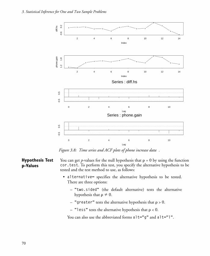
3. Statistical Inference for One and Two Sample Problems
Hypothesis Test
p-Values
You can get p-values for the null hypothesis that r = 0 by using the functioncor.test. To perform this test, you specify the alternative hypothesis to betested and the test method to use, as follows:
� alternative= specifies the alternative hypothesis to be tested.There are three options:
� "two.sided" (the default alternative) tests the alternativehypothesis that r Þ 0.
� "greater" tests the alternative hypothesis that r > 0.
� "less" tests the alternative hypothesis that r < 0.
You can also use the abbreviated forms alt="g" and alt="l".
Figure 3.8: Time series and ACF plots of phone increase data .
• • •• •
•
• •• •
••
•
•
Index
diff.
hs
2 4 6 8 10 12 14
-0.6
0.2
• •
•• • •
••
• •
• •
• •
Index
phon
e.ga
in
2 4 6 8 10 12 14
1.2
1.8
Lag
0 2 4 6 8 10
-0.5
0.5
Series : diff.hs
Lag
0 2 4 6 8 10
-0.5
0.5
Series : phone.gain
70

Correlation
� method= specifies which of the following methods is used:
� "pearson" (the default) uses the standard Pearson sample cor-relation coefficient.
� "kendall" uses the rank-based Kendall�s t measure of correla-tion.
� "spearman" uses the rank-based Spearman�s r measure of cor-relation.
You can abbreviate these methods by using enough of the characterstring to determine a unique match; here "p", "k", and "s" work.
Because both Kendall�s t and Spearman�s r methods are based on ranks, theyare not so sensitive to outliers and non-normality as the standard Pearsonestimate.
Here is a simple use of cor.test to test the alternative hypothesis that thereis a positive correlation in the phone gain data. We use the default choice ofthe classical Pearson estimate with the one-sided alternative alt="g":
> cor.test(diff.hs,phone.gain,alt="g")
Pearson product-moment correlation
data: diff.hs and phone.gain
t = 1.9155, df = 12, p-value = 0.0398
alternative hypothesis: true coef is greater than 0
sample estimates:
cor
0.4839002
You get a normal theory t-statistic having the modest value of 1.9155, and ap-value of .0398. The estimate of r is .48, to two decimal places. There are14 bivariate observations, and since the mean is estimated for each sampleunder the null hypothesis that r > 0, the number of degrees of freedom (df) is12.
Since your EDA plots reveal two obvious bivariate outliers in the phone gaindata, the non-parametric alternatives, either Kendall�s t or Spearman�s r, arepreferable in determining p-values for this case. Using Kendall�s method, weobtain the following results:
> cor.test(diff.hs,phone.gain,alt="g",method="k")
71

3. Statistical Inference for One and Two Sample Problems
Kendall�s rank correlation tau
data: diff.hs and phone.gain
normal-z = 2.0256, p-value = 0.0214
alternative hypothesis: true tau is greater than 0
sample estimates:
tau
0.4065934
The p-value obtained from Kendall�s method is smaller than that obtainedfrom the Pearson method. The null hypothesis is rejected at a level of 0.05.Spearman�s r, by contrast, yields a p-value similar to that of the standardPearson method.
Warning The values returned for �tau" and �rho" (.407 and .504, respectively, for thephone gain data) do not provide unbiased estimates of the true correlation r.Transformations of �tau" and �rho" are required to obtain unbiased estimatesof r.
Point Estimates
and Confidence
Intervals for r
You may want an estimate of r, or a confidence interval for r. Thefunction cor.test gives you the classical sample correlation coefficientestimate r of r, when you use the default Pearson�s method. However,cor.test does not provide you with a robust estimate of r, (since neitherKendall�s t or Spearman�s r provide an unbiased estimate of r). Furthermore,cor.test does not provide any kind of confidence interval for r.
To obtain a robust point estimate of r, use the function cor with a non-zerovalue for the optional argument trim=. You should specify a fraction abetween 0 and .5 for the value of this argument. This results in a robustestimate which consists of the ordinary sample correlation coefficient basedon the fraction (1-a) of the data remaining after �trimming" away a fractiona. In most cases, set trim=.2. If you think your data contain more than20% outliers, you should use a larger fraction in place of .2. The defaultvalue is trim=0, which yields the standard Pearson sample correlationcoefficient.
Applying cor to the phone gain data, you get:
> cor(diff.hs,phone.gain,trim=.2)
[1] 0.715215
Comparing this robust estimate to our earlier value for r obtained usingcor.test, we see the robust estimate yields a larger estimate of r. This iswhat you expect, since the two outliers cause the standard sample correlationcoefficient to have a value smaller than that of the �bulk" of the data.
ρ
72

References
To obtain a confidence interval for r, we�ll use the following procedure (as inSnedecor and Cochran (1980)). First, transform r using Fisher�s �z-transform,� which consists of taking the inverse hyperbolic tangent transformz = atanh(r). Then, construct a confidence interval for the correspondingly
transformed true correlation coefficient . Finally, transform
this interval back to the original scale by transforming each endpoint of thisinterval with the hyperbolic tangent transformation tanh.
To implement the procedure just described as an S-PLUS function, create thefunction cor.confint as follows:
> cor.confint <- function(x, y, conf.level = .95, trim = 0)
+ {
+ z <- atanh(cor(x, y, trim))
+ b <- qnorm((1 - conf.level)/2)/(length(x) - 3)^.5
+ ci.z <- c(z - b, z + b)
+ conf.int <- tanh(ci.z)
+ conf.int
+ }
You can now use your new function cor.confint on the phone gain data:
> cor.confint(diff.hs,phone.gain)
[1] 0.80722631 -0.06280418
> cor.confint(diff.hs,phone.gain,trim=.2)
[1] 0.9028239 0.2962303
When you use the optional argument trim=.2, you are basing theconfidence interval on a robust estimate of r, and consequently you get arobust confidence interval. Since the robust estimate has the value .72, whichis larger than the standard (non-robust) estimate value of .48, you should bereassured to get an interval which is shifted upward, and is also shorter, thanthe non-robust interval you got by using cor.confint with the defaultoption trim=0.
3.6 REFERENCESBishop, Y. M. M. and Fienberg, S. J. and Holland, P. W. (1980). DiscreteMultivariate Analysis: Theory and Practice. The MIT Press, Cambridge, MA.
Box, G.E.P. and Hunter, W.G. and Hunter, J.S. (1978). Statistics forExperimenters: An Introduction to Design, Data Analysis and Model Building.John Wiley, New York.
Conover, W. J. (1980). Practical Nonparametric Statistics, 2nd edition. JohnWiley, New York.
ρ ρ( )atanh=
73

3. Statistical Inference for One and Two Sample Problems
Heidelberger, P. and Welch, P. D. (1981). A Spectral Method for ConfidenceInterval Generation and Run-length Control in Simulations.Communications of the ACM, 24:233�245.
Hogg, R. V. and Craig, A. T. (1970). Introduction to Mathematical Statistics,3rd edition. Macmillan, Toronto, Canada.
Mood, A. M. and Graybill, F. A. and Boes, D. C. (1974). Introduction to theTheory of Statistics, 3rd edition. McGraw-Hill, New York.
Snedecor, G. W. and Cochran, W. G. (1980). Statistical Methods, 7th edition.Iowa State University Press, Ames, IA.
74

GOODNESS OF FIT TESTS 44.1 Cumulative Distribution Functions 77
4.2 The Chi-Square Test of Goodness of Fit 79
4.3 The Kolmogorov-Smirnov Test 82
4.4 One Sample Tests 83
Composite Tests for a Family of Distributions 85
4.5 Two Sample Tests 87
4.6 References 88
75

4. Goodness of Fit Tests
76

GOODNESS OF FIT TESTS 4Most S-PLUS functions for hypothesis testing assume a certain distributionalform�often normal�and then use data to make conclusions about certainparameters of the distribution�often the mean or variance. In chapter 3,Statistical Inference for One and Two Sample Problems, we describe EDAtechniques to informally test the assumptions of these procedures. Goodnessof fit (GOF) tests are another, more formal, tool to assess the evidence forassuming a certain distribution.
There are two types of GOF problems�corresponding to the number ofsamples�which ask the following questions:
1. One sample. Does the sample arise from a hypothesized distribution?
2. Two sample. Do two independent samples arise from the samedistribution?
S-PLUS implements the two best known GOF tests:
� Chi-square, in the chisq.gof function.
� Kolmogorov-Smirnov, in the ks.gof function.
The chi-square test applies only in the one-sample case; Kolmogorov-Smirnov can be used in both the one-sample and the two-sample cases. Thischapter describes both tests, together with a graphical function,cdf.compare, that can be used in both the one-sample and two-samplecases as an exploratory tool for evaluating goodness of fit.
4.1 CUMULATIVE DISTRIBUTION FUNCTIONSFor a random variable X, a cumulative distribution function (cdf), F(x) =P[X # x], assigns a measure (between 0 and 1) of the probability that X # x.If X1, �, Xn form a random sample from a continuous distribution, withobserved values x1, �, xn, an empirical distribution function Fn can be
defined for all x, , so that Fn(x) is the proportion of observed
values less than or equal to x. The empirical distribution function estimatesthe unknown cdf. To decide whether two samples arise from the sameunknown distribution, a natural procedure is to compare their empiricaldistribution functions. Likewise, for one sample, you can compare itsempirical distribution function with a hypothesized cdf.
A graphical comparison of either one empirical distribution function with aknown cdf, or of two empirical distribution functions, can be obtained easilyin S-PLUS using the function cdf.compare.
∞ x ∞< <–
77

4. Goodness of Fit Tests
For example, consider the plot shown in figure 4.1. In this example, theempirical distribution function and a hypothetical cdf are quite close. Thisplot is produced using the cdf.compare function as follows:
> z <- rnorm(100)
> cdf.compare(z, distribution="normal")
You may also compare distributions using quantile-quantile plots (Q-Qplots) generated by either of the following functions:
� qqnorm to compare one sample with a normal distribution
� qqplot to compare two samples
For our normal sample z, qqnorm(z) produces the plot shown in figure 4.2.Departures from linearity show how the sample differs from the normal, orhow the two sample distributions differ. To compare samples with
Figure 4.1: The empirical distribution function of a sample of size 100generated from a N(0,1) distribution. The dotted line is the smoothedtheoretical N(0,1) distribution evaluated at the sample points.
Empirical and Hypothesized CDFs
-2 -1 0 1 2
0.0
0.2
0.4
0.6
0.8
1.0
dotted line is the smoothed hypothesized continuous cdf
78

The Chi-Square Test of Goodness of Fit
distributions other than the normal, you may produce Q-Q plots using thefunction ppoints. For more details, see the chapter Traditional Graphics inthe S-PLUS Programmer�s Guide.
In many cases, the graphical conclusions drawn from cdf.compare or theQ-Q plots make more formal tests such as the chi square or Kolmogorov-Smirnov unnecessary. For example, consider the two empirical distributionscompared in figure 4.3�they clearly have different distribution functions:
> x <- rnorm(30)
> y <- runif(30)
> cdf.compare(x,y)
4.2 THE CHI-SQUARE TEST OF GOODNESS OF FITThe chi-square test, the oldest and best known goodness-of-fit test, is a one-sample test that examines the frequency distribution of n observationsgrouped into k classes. The observed counts ci in each class are compared tothe expected counts Ci from the hypothesized distribution. The test statistic,
due to Pearson, is
Figure 4.2: A qqnorm plot of a sample from a normal distribution.
•
••
•
•
•
•
••
•
••
•
•
•
•
• •
•
••
•
• •••
•
•
•
•
••
•
••
•
•
•
•
•
•
•
•
•
•
•
•
•
•
•
•
•
••
•
•
•
•
•
•
••
•
•
•
•
•
•
•
•
•
•
•
•
•
•
••
•
•
•
•
•
••
••
•
•
•
•
•
•
••
•
•
•
•
•
Quantiles of Standard Normal
z
-2 -1 0 1 2
-3-2
-10
12
79

4. Goodness of Fit Tests
.
Under the null hypothesis that the sample comes from the hypothesized
distribution, it has a distribution with k-1 degrees of freedom. For any
significance level a, reject the null hypothesis if is greater than the critical
value n for which .
You perform the chi-square goodness of fit test with the chisq.goffunction. In the simplest case, you specify a test vector and a hypothesizeddistribution:
> z.chisq <- chisq.gof(z, distribution="normal")
> z.chisq
Chi-square Goodness of Fit Test
data: z
Chi-square = 8.94, df = 12,
p-value = 0.708
Figure 4.3: Two clearly different empirical distribution functions.
Comparison of Empirical cdfs of x and y
dotted line is cdf of y-2 -1 0 1 2
0.0
0.2
0.4
0.6
0.8
1.0
χ2 ci Ci–( )2 Ci⁄i 1=
k
∑=
χ2
χ2
P χ2 ν>( ) α=
80

The Chi-Square Test of Goodness of Fit
alternative hypothesis:
True cdf does not equal the normal Distn.
for at least one sample point.
Since we created z as a random sample from a normal distribution, it is notsurprising that we cannot reject the null hypothesis. If we hypothesize adifferent distribution, we see that the chi-square correctly rejects thehypothesis:
> chisq.gof(z, distribution="exponential")
Chi-square Goodness of Fit Test
data: z
Chi-square = 324.84, df = 12,
p-value = 0
alternative hypothesis:
True cdf does not equal the exponential Distn.
for at least one sample point.
The allowable values for the distribution argument are the followingstrings (the default is "normal"):
"beta" "binomial" "cauchy" "chisquare"
"exponential" "f" "gamma" "geometric"
"hypergeometric" "lognormal" "logistic" "negbinomial"
"normal" "poisson" "t" "uniform"
"weibull" "wilcoxon"
When the sample being tested is from a continuous distribution, one factoraffecting the outcome is the choice of partition for determining the groupingof the observations. This becomes particularly important when the expectedcount in one or more cells drops below 1, or the average expected cell countdrops below five (Snedecor and Cochran (1980), p. 77). You can control thechoice of partition using either the n.classes or cut.points argument tochisq.gof. By default, chisq.gof uses a default value for n.classes dueto Moore (1986).
Use the n.classes argument to specify the number of equal-width classes:
> chisq.gof(z, n.classes=5)
Use the cut.points argument to specify the end points of the cells; thespecified points should span the observed values:
> cuts.z <- c(floor(min(z))-1, -1,0,1, ceiling(max(z))+1)
> chisq.gof(z, cut.points=cuts.z)
81

4. Goodness of Fit Tests
Chi-square tests apply to any type of variable: continuous, discrete, or acombination of these. For large sample sizes (n $ 50), if the hypothesizeddistribution is discrete, the chi-square is the only valid test. In addition, thechi-square test easily adapts to the situation when parameters of adistribution are estimated. However, especially for continuous variables,information is lost by grouping the data.
When the hypothesized distribution is continuous, the Kolmogorov-Smirnovtest is more likely to reject the null hypothesis when it should; it is morepowerful than the chi-square test.
4.3 THE KOLMOGOROV-SMIRNOV TESTSuppose F1 and F2 are two cdfs. In the one-sample situation, F1 is the
empirical distribution function, and F2 is a hypothesized cdf. In the two-sample situation, F1 and F2 are both empirical distribution functions.
Possible hypotheses and alternatives concerning these cdfs are:
� Two-sided:
H0: F1(x) = F2(x) for all x
HA: F1(x) Þ F2(x) for at least one value of x.
� One-sided (�less� alternative):
H0: F1(x) $ F2(x) for all x
HA: F1(x) < F2(x) for at least one value of x.
� One-sided (�greater� alternative):
H0: F1(x) # F2(x) for all x
HA: F1(x) > F2(x) for at least one value of x.
The Kolmogorov-Smirnov test is a method for testing the above hypotheses.Corresponding to each alternative hypothesis is a Kolmogorov-Smirnov teststatistic, as follows:
� Two-sided Test:
� Less Alternative:
� Greater Alternative:
If the test statistic is greater than some critical value, the null hypothesis isrejected.
T supx F1 x( ) F2 x( )–=
T- supx F2 x( ) F1 x( )–=
T+ supx F1 x( ) F2 x( )–=
82

One Sample Tests
To perform a KS test, use the function ks.gof. By default, the one-sampleks.gof test compares the sample x to a normal with mean mean(x) andstandard deviation sqrt(var(x)):
> ks.gof(z)
One sample Kolmogorov-Smirnov Test of Composite Normality
data: z
ks = 0.0457, p-value = 0.5
alternative hypothesis:
True cdf does not equal the normal Distn.
for at least one sample point.
sample estimates:
mean of x standard deviation of x
-0.04593973 1.103777
Warning messages:
The Dallal-Wilkinson approximation, used to calculate
the p-value in testing composite normality,
is most accurate for p-values <= 0.10 .
The calculated p-value is 0.881
and so is set to 0.5 . in: dall.wilk(test, nx)
In the one-sample case, ks.gof can test any of the three alternativehypotheses ("two-sided", "greater", "less"). In the two-sample case,ks.gof can test only the two-sided hypothesis. The default hypothesizeddistribution is the normal, as for the chisq.gof function. You can specify adifferent distribution using the distribution argument. Allowable valuesfor the distribution argument are as follows:
"beta" "binomial" "cauchy" "chisquare"
"exponential" "f" "gamma" "geometric"
"hypergeometric" "lognormal" "logistic" "negbinomial"
"normal" "poisson" "t" "uniform"
"weibull" "wilcoxon"
4.4 ONE SAMPLE TESTSIn a real situation, we do not know the true source of the data. Suppose,instead, that we think the underlying distribution is chi-square with 2 degreesof freedom. The KS test gives strong evidence against this assumption:
> ks.gof(z,alternative="greater",dist="chisquare",df=2)
83

4. Goodness of Fit Tests
One-sample Kolmogorov-Smirnov Test;
hypothesized distribution = chisquare
data: z
ks = 0.4741, p-value = 0
alternative hypothesis: True cdf is greater than the
chisquare Distn. for at least one sample point.
Figure 4.4, created as follows, further shows that this assumption is notreasonable:
> cdf.compare(z, dist="chisquare", df=2)
The chisq.gof test gives further confirmation:
> chisq.gof(z,dist="chisquare",n.param.est=0,df=2)
Figure 4.4: Like the previous figure, except the dotted line shows a chi-square cdf with 2 degrees of freedom.
Empirical and Hypothesized chisquare CDFs
solid line is the empirical d.f.-4 -2 0 2
0.0
0.2
0.4
0.6
0.8
1.0
84

One Sample Tests
Chi-square Goodness of Fit Test
data: z
Chi-square = 282.98, df = 12, p-value = 0
alternative hypothesis: True cdf does not equal the
chisquare Distn. for at least one sample point.
Note that chisq.gof tests only the two sided alternative.
Composite
Tests for a
Family of
Distributions
When the parameters are estimated from the sample, rather than specified inadvance, the tests described above are no longer adequate. Different tables ofcritical values are needed. In fact, for the KS test, the tables vary for differentdistributions, parameters estimated, methods of estimation, and sample sizes.The null hypothesis is now composite: rather than hypothesizing that the datahave a distribution with specific parameters, we hypothesize only that thedistribution belongs to the family of distributions with a certain form, suchas normal. This family of distributions results from allowing all possibleparameter values.
The two functions ks.gof and chisq.gof use different strategies to solvecomposite tests: ks.gof explicitly calculates the required parameters in twocases (described below), but otherwise forbids composite hypotheses, whilechisq.gof requires the user to pass both the number of estimatedparameters and the estimates themselves as arguments, then reduces thedegrees of freedom for the chi-square by the number of estimated parameters.
The function ks.gof estimates parameters in the following two cases:
� Normal, with both mean and variance estimated.
� Exponential, with mean estimated.
As an example, we test whether we can reasonably assume that the Michelsondata (see the section One Sample: Distribution Shape, Location, and Scaleon page 51) arises from a normal distribution. We start with an exploratoryplot using cdf.compare (figure 4.5), and then use ks.gof with estimatedmean and variance:
> cdf.compare(mich, dist="normal", mean=mean(mich),
+ sd=sqrt(var(mich)))
> ks.gof(mich,dist="normal")
One-sample Kolmogorov-Smirnov Test of Composite Normality
data: mich
ks = 0.1793, p-value = 0.0914
alternative hypothesis: True cdf does not equal
the normal Distn. for at least one sample point.
85

4. Goodness of Fit Tests
For the function chisq.gof, if parameters are estimated, the degrees offreedom depend on the method of estimation. In practice, you may estimatethe parameters from the original (that is, not grouped) data, and then set theargument n.param.est to the number of parameters estimated. Thefunction then subtracts one degree of freedom for each parameter estimated.
In truth, if the parameters are estimated by maximum likelihood, the degreesof freedom are bounded between (m-1) and (m-1-k), where m is the numberof cells, and k is the number of parameters estimated. Therefore, especiallywhen the sample size is small, it is important to compare the test statistic tothe chi-square distribution with both (m-1) and (m-1-k) degrees of freedom.See Kendall and Stuart (1979), for a more complete discussion.
We again test the normal assumption for the Michelson data usingchisq.gof:
> chisq.gof(mich, dist="normal", n.param.est=2,
+ mean=mean(mich), sd=sqrt(var(mich)))
Figure 4.5: Exploratory plot of cdf of mich data.
Empirical and Hypothesized normal CDFs
solid line is the empirical d.f.700 800 900 1000
0.0
0.2
0.4
0.6
0.8
1.0
86

Two Sample Tests
Chi-square Goodness of Fit Test
data: mich
Chi-square = 8.7, df = 4, p-value = 0.0691
alternative hypothesis: True cdf does not equal
the normal Distn. for at least one sample point.
Warning messages:
Expected counts < 5. Chi-square approximation may not
be appropriate. in: chisq.gof(mich, dist = "normal",
n.param.est = 2, mean = mean(mich), sd = sqrt( ....
Both goodness-of-fit tests return results which make us suspect the nullhypothesis, but don�t allow us to firmly reject it at 95% or 99% confidencelevels.
Note that the distribution theory of the chi-square test is a large sampletheory. Therefore when any expected cell counts are small, chisq.gof issuesa warning message. You should regard p-values with caution in this case.
4.5 TWO SAMPLE TESTSIn the two-sample case, you can use ks.gof as for the one-sample case (withthe second sample y filling in for the hypothesized distribution).
The assumptions of the two-sample KS test are:
� the samples are random samples,
� the two samples are mutually independent, and
� the data are measured on at least an ordinal scale.
In addition, the test gives exact results only if the underlying distributions arecontinuous.
For example, compare the cdfs of vectors x and y generated from a normaland exponential distribution, respectively:
> x <- rnorm(30)
> y <- rexp(100)
> qqplot(x,y)
> cdf.compare(x,y)
Figure 4.6 shows a Q-Q plot which is not linear, and cdfs which are quitedifferent. This graphical evidence is verified by a formal KS test:
> ks.gof(x,y)
87

4. Goodness of Fit Tests
Two-Sample Kolmogorov-Smirnov Test
data: x and y
ks = 0.3667, p-value = 0.0028
alternative hypothesis:
cdf of x does not equal the
cdf of y for at least one sample point.
4.6 REFERENCESKendall, M. G. and Stuart, A. (1979). The Advanced Theory of Statistics, 4thedition, 2:Inference and Relationship. Oxford University Press, New York.
Moore, D. S. (1986). Tests of Chi-Squared Type. In D'Agostino, R. B. andStevens, M. A.", editors, Goodness-of-Fit Techniques. Marcel Dekker, NewYork.
Snedecor, G. W. and Cochran, W. G. (1980). Statistical Methods, 7thedition. Iowa State University Press, Ames, Iowa.
Figure 4.6: A normal and exponential (dotted line) sample compared.
• •• •
• •• •••
•
•••• ••
••••••• •
•••
•
•
x
y
-1 0 1 2
01
23
Comparison of Empirical cdfs of x and y
dotted line is cdf of y
-1 0 1 2 3
0.0
0.2
0.4
0.6
0.8
1.0
88

STATISTICAL INFERENCE FOR
COUNTS AND PROPORTIONS 55.1 Proportion Parameter for One Sample 92
Hypothesis Testing 92
Confidence Intervals 93
5.2 Proportion Parameters for Two Samples 93
Hypothesis Testing 94
Confidence Intervals 95
5.3 Proportion Parameters for Three or More Samples 96
Hypothesis Testing 97
Confidence Intervals 98
5.4 Contingency Tables and Tests for Independence 98
The Chi-Square and Fisher Tests of Independence 99
The Chi-Square Test of Independence 102
Fisher�s Exact Test of Independence 103
The Mantel-Haenszel Test of Independence 103
McNemar Test for Symmetry Using Matched Pairs 105
5.5 References 106
89

5. Statistical Inference for Counts and Proportions
90

STATISTICAL INFERENCE FOR COUNTS AND
PROPORTIONS 5This chapter shows you how to use S-PLUS statistical inference functions fortwo types of problems that involve counts or proportions. With thesefunctions, you can obtain confidence intervals for the unknown populationparameters and p-values for hypothesis tests of the parameter values.
The first type of problem is one where you have one or more samples, or setsof trials, in which the count for each sample represents the number of timesthat a certain interesting outcome occurs. By common convention, we referto the occurrence of the outcome of interest as a �success�. For example, ifyou play roulette 100 times at a casino, and you bet on red each time, you areinterested in counting the number of times that the color red comes up. Thiscount is a number between 0 and 100. When you divide this count by 100you get a proportion (that is, a number between 0 and 1). This proportion isa natural estimate of the probability that red comes up on the roulette wheel.
Another example is provided by the famous Salk vaccine trials. These trialsinvolved two groups, one of which received the vaccine and one of whichreceived a placebo. For each group, the count of interest was the number ofindividuals who contracted polio. The ratio of the number of individualswho contracted polio to the total number of individuals in the group is aproportion that provides a natural estimate of the probability of contractingpolio within that group.
The underlying probability model for problems of this first type is thebinomial distribution. For each set of trials i, this distribution is characterizedby the number of trials and the probability pi that a success occurs on each
trial. This probability is called a proportion parameter. Your main interest is inmaking statistical inference statements concerning the probabilities p1,
p2, �, pm of occurrence of the event of interest for each of the m sets of
trials.
The second type of problem is one where you have counts on the number ofoccurrences of several possible outcomes for each of two variables. Forexample, you may be studying three types of cancer and three types of diet(such as low, medium and high fat diets). The two variables of interest maybe �type of cancer� and �type of diet�. For a fixed set of individuals, you havecounts on the number of individuals who fall jointly in each of the categoriesdefined by the simultaneous occurrence of a type of cancer and a dietclassification. For problems of this kind, the data is arranged in a two-waytable called a contingency table.
91

5. Statistical Inference for Counts and Proportions
In this second kind of problem, your main interest is to determine whetherthere is any association between the two variables of interest. The probabilitymodel for such problems is one of statistical independence between the twovariables.
The first three sections of this chapter cover the first type of problemdescribed above, for which the proportion parameters are the probabilities ofsuccess, p1, p2, �, pm in m sets of binomial trials. The last section covers the
second type of problem, where you are interested in testing the nullhypothesis of independence between two variables.
5.1 PROPORTION PARAMETER FOR ONE SAMPLEWhen you play roulette and bet on red, you expect your probability ofwinning to be close to, but slightly less than, 0.5. You expect this because (inthe United States) a roulette wheel has 18 red slots, 18 black slots, and twoadditional slots labeled �0� and �00�, for a total of 38 slots into which theball can fall. Thus, for a �fair� (that is, perfectly balanced) wheel, you expectthe probability of red to be p0 = 18/38 = .474. You hope that the house is notcheating you by altering the roulette wheel so that the probability of red isless than .474.To test whether a given sample has a particular proportion parameter, use thebinom.test function.
Setting Up the
Data
In the roulette case there is little to do, since the only data are the number nof trials and the number x of successes. These two values can be directlysupplied as arguments to binom.test, as shown in the examples below.
Hypothesis
Testing
You can test the null hypothesis that p = p0 using the function binom.test.
For example, if you bet on red 100 times and red comes up 42 times, you geta p-value for this null hypothesis against the two-sided alternative thatpÞ .474 as follows:
> binom.test(42,100,p=.474)$p.value
[1] 0.3167881
The two-sided alternative is the default alternative for binom.test. You canget a p-value for a one-sided alternative by using the optional argumentalt=. For example, in the roulette wheel example you are concerned that thehouse might cheat you in some way so that p < p0. Use the following to test
the null hypothesis against this one-sided alternative:
> binom.test(42,100,p=.474,alt="l")$p.value
[1] 0.1632416
92

Proportion Parameters for Two Samples
Here alt="l" specifies the �less than� alternative p < p0. To specify the
�greater than� alternative p > p0, use alt="g".
The default for the optional argument p=, which specifies the null hypothesisvalue for p, is p=.5. For example, suppose you toss a coin 1000 times, withheads coming up 473 times. To test the coin for �fairness;� that is, to test thatthe probability of heads equals .5, use the following:
> binom.test(473,1000)$p.value
[1] 0.09368729
Confidence
Intervals
The function binom.test does not compute a confidence interval for theprobability p of success. You can get a confidence interval for p by using thefunction prop.test. For example, the following shows how to obtain the95% confidence interval for p:
> prop.test(45,100)$conf.int
[1] 0.3514281 0.5524574
attr(, "conf.level"):
[1] 0.95
The function prop.test uses a normal approximation to the binomialdistribution for such computations.
You get different confidence intervals by using the optional argumentconf.level= with different values. For example, to get a 90% confidenceinterval:
> prop.test(45,100,conf.level=.9)$conf.int
[1] 0.3657761 0.5370170
attr(, "conf.level"):
[1] 0.9
5.2 PROPORTION PARAMETERS FOR TWO SAMPLESIn the Salk vaccine trials, two large groups were involved in the placebo-control phase of the study. The first group, which received the vaccination,consisted of 200,745 individuals. The second group, which received aplacebo, consisted of 201,229 individuals. There were 57 cases of polio in thefirst group and 142 cases of polio in the second group.
You assume a binomial model for each group, with a probability p1 of
contracting polio in the first group and a probability p2 of contracting polio
in the second group. You are mainly interested in knowing whether or notthe vaccine is effective. Thus you are mainly interested in knowing therelationship between p1 and p2.
93

5. Statistical Inference for Counts and Proportions
You can use prop.test to obtain hypothesis test p-values concerning thevalues of p1 and p2, and to obtain confidence intervals for the difference
between the values p1 and p2.
Setting Up the
Data
The first two arguments to prop.test are vectors containing, respectively, thenumber of successes and the total number of trials. For consistency with theone-sample case, we name these vectors x and n. In the case of the Salkvaccine trials, a �success� corresponds to contracting polio (although onehardly thinks of this as a literal success!) Thus, you create the vectors x and nas follows: > x <- c(57,142)
> n <- c(200745,201229)
Hypothesis
Testing
For two-group problems, you can use either of two null hypotheses: an equalprobabilities null hypothesis that p1 = p2, with no restriction on the common
value of these probabilities other than that they be between 0 and 1, or acompletely specified probabilities null hypothesis, where you provide specificprobabilities for both p1 and p2, and test whether the true probabilities are
equal to those hypothesized.
The Equal
Probabilities Null
Hypothesis
When using the equal probabilities null hypothesis, a common alternativehypothesis is the two-sided alternative p1 Þ p2. These null and alternative
hypotheses are the defaults for prop.test.
In the Salk vaccine trials, your null hypothesis is that the vaccine has noeffect. For the two-sided alternative that the vaccine has some effect, eitherpositive or negative, you get a p-value by extracting the p.value componentof the list returned by prop.test:
> prop.test(x,n)$p.value
[1] 2.86606e-09
The extremely small p-value clearly indicates that the vaccine has some effect.
To test the one-sided alternative that the vaccine has a positive effect; that is,that p1 , p2, use the argument alt="l" to prop.test:
> prop.test(x,n,alt="l")$p.value
[1] 1.43303e-09
Here the p-value is even smaller, indicating that the vaccine is highly effectivein protecting against the contraction of polio.
94

Proportion Parameters for Two Samples
Completely
Specified Null
Hypothesis
Probabilities
You can also use prop.test to test �completely� specified null hypothesisprobabilities. For example, suppose you have some prior belief that theprobabilities of contracting polio with and without the Salk vaccine arep01 = .0002 and p02 = .0006, respectively. Then you supply these null
hypothesis probabilities as a vector object, using the optional argument p=.The p-value returned is for the joint probability that both probabilities areequal to the hypothesized probabilities; that is, .0002 and .0006 . > prop.test(x,n,p=c(.0002,.0006))$p.value
[1] 0.005997006
The above p-value is very small and indicates that the null hypothesis that thejoint probability that the underlying population probabilities with andwithout the Salk vaccine are .0002 and .0006 is very unlikely and should berejected.
Confidence
Intervals
You obtain a confidence interval for the difference p1 - p2 in the probabilities
of success for the two samples by extracting the conf.int component ofprop.test. For example, to get a 95% confidence interval for the differencein probabilities for the Salk vaccine trials:
> prop.test(x,n)$conf.int
[1] -0.0005641810 -0.0002792617
attr(, "conf.level"):
[1] 0.95
The 95% confidence level is the default confidence level for prop.test. Youget a different confidence level by using the optional argumentconf.level=. For example, to get a 99% confidence interval, use:
> prop.test(x,n,conf.level=.99)$conf.int
[1] -0.0006073705 -0.0002360723
attr(, "conf.level"):
[1] 0.99
You get a confidence interval for the difference p1 - p2 by using prop.test
only when you use the default null hypothesis that p1 = p2.
You get all the information provided by prop.test as follows:
> prop.test(x,n,conf.level=.90)
95

5. Statistical Inference for Counts and Proportions
2-sample test for equality of proportions with
continuity correction
data: x out of n
X-squared = 35.2728, df = 1, p-value = 0
alternative hypothesis: two.sided
90 percent confidence interval:
-0.0005420769 -0.0003013659
sample estimates:
prop�n in Group 1 prop�n in Group 2
0.0002839423 0.0007056637
5.3 PROPORTION PARAMETERS FOR THREE OR MORE SAMPLESSometimes you may have three or more samples of subjects, with each subjectcharacterized by the presence or absence of some characteristic. Analternative, but equivalent, terminology is that you have three or more sets oftrials, with each trial resulting in a success or failure. For example, considerthe data shown in table 5.1 for four different studies of lung cancer patients,as presented by Fleiss (1981).
Each study has a certain number of patients, as shown in the second columnof the table, and for each study a certain number of the patients weresmokers, as shown in the third column of the table. For this data, you areinterested in whether the probability of a patient being a smoker is the samein each of the four studies, that is, whether each of the studies involvepatients from a homogeneous population.
Setting Up the
Data
The first argument to prop.test is a vector containing the number ofsubjects having the characteristic of interest for each of the groups (or thenumber of successes for each set of trials). The second argument to
Table 5.1: Smoking status among lung cancer patients in four studies.
Study Number of Patients Number of Smokers
1 86 83
2 93 90
3 136 129
4 82 70
96

Proportion Parameters for Three or More Samples
prop.test is a vector containing the number of subjects in each group (orthe number of trials for each set of trials). As in the one and two sample cases,we call these vectors x and n.
For the smokers data in table 5.1, you create the vectors x and n as follows:
> x <- c(83,90,129,70)
> n <- c(86,93,136,82)
Hypothesis
Testing
For problems with three or more groups, you can use either an equalprobabilities null hypothesis or a completely specified probabilities nullhypothesis.
The Equal
Probabilities Null
Hypothesis
In the lung cancer study, the null hypothesis is that the probability of being asmoker is the same in all groups. Because the default null hypothesis forprop.test is that all groups (or sets of trials) have the same probability ofsuccess, you get a p-value as follows:
> prop.test(x,n)$p.value
[1] 0.005585477
The p-value of .006 is highly significant, so you can not accept the nullhypothesis that all groups have the same probability that a patient is asmoker. To see all the results returned by prop.test, use:
> prop.test(x,n)
4-sample test for equality of proportions without
continuity correction
data: x out of n
X-squared = 12.6004, df = 3, p-value = 0.0056
alternative hypothesis: two.sided
sample estimates:
prop�n in Group 1 prop�n in Group 2 prop�n in Group 3
0.9651163 0.9677419 0.9485294
prop�n in Group 4
0.8536585
Completely
Specified Null
Hypothesis
Probabilities
If you want to test a completely specified set of null hypothesis probabilities,you need to supply the optional argument p=, with the value of thisargument being a vector of probabilities having the same length as the firsttwo arguments, x and n.
97

5. Statistical Inference for Counts and Proportions
For example, in the lung cancer study, to test the null hypothesis that the firstthree groups have a common probability .95 of a patient being a smoker,while the fourth group has a probability .90 of a patient being a smoker,create the vector p as follows, the use it as an argument to prop.test:
> p <- c(.95,.95,.95,.90)
> prop.test(x,n,p)$p.value
[1] 0.5590245
Warning messages:
Expected counts < 5. Chi-square approximation may not be
appropriate.
Alternatively, you could use
prop.test(x,n,p=c(.95,.95,.95,.90))$p.value
Confidence
Intervals
Confidence intervals are not computed by prop.test when you have threeor more groups (or sets of trials).
5.4 CONTINGENCY TABLES AND TESTS FOR INDEPENDENCEThe Salk vaccine trials in the early 1950s resulted in the data presented intable 5.2.
There are two categorical variables for the Salk trials: vaccination status,which has the two levels �vaccinated� and �placebo,� and polio status, whichhas the three levels �no polio,� �non-paralytic polio,� and �paralytic polio.�Of 200,745 individuals who were vaccinated, 24 contracted non-paralyticpolio, 33 contracted paralytic polio, and the remaining 200,688 did notcontract any kind of polio. Of 201,229 individuals who received the placebo,27 contracted non-paralytic polio, 115 contracted paralytic polio, and theremaining 201,087 did not contract any kind of polio.
Table 5.2: Contingency table of Salk vaccine trials data.
No PolioNon-paralytic Polio
Paralytic Polio
Totals
Vaccinated 200,688 24 33 200,745
Placebo 201,087 27 115 201,229
Totals 401,775 51 148 401,974
98

Contingency Tables and Tests for Independence
Tables such as table 5.2 are called contingency tables. A contingency tablelists the number of counts for the joint occurrence of two levels (or possibleoutcomes), one level for each of two categorical variables. The levels for oneof the categorical variables correspond to the columns of the table, and thelevels for the other categorical variable correspond to the rows of the table.
When working with contingency table data, your primary interest is mostoften determining whether there is any association in the form of statisticaldependence between the two categorical variables whose counts are displayedin the table. The null hypothesis is that the two variables are statisticallyindependent. You can test this null hypothesis with the functionschisq.test and fisher.test. The function chisq.test is based onthe classic chi-square test statistic, and the associated p-value computationentails some approximations. The function fisher.test computes anexact p-value for tables having at most 10 levels for each variable. Thefunction fisher.test also entails a statistical conditioning assumption.
For contingency tables involving confounding variables, which are variablesrelated to both variables of interest, you can test for independence using thefunction mantelhaen.test, which performs the Mantel-Haenszel test. Forcontingency tables involving matched pairs, use the function mcnemar.testto perform McNemar�s chi-square test.
The functions for testing independence in contingency tables do notcompute confidence intervals, only p-values and the associated test statistic.
The Chi-Square
and Fisher
Tests of
Independence
The chi-square and Fisher�s exact tests are familiar methods for testingindependence. The Fisher test is often recommended when expected countsin any cell are below 5, as the chi-square probability computation becomesincreasingly inaccurate when the expected counts in any cell are low. (S-PLUS
produces a warning message in that case). Other factors may also influenceyour choice of which test to use, however. Refer to a statistics text for furtherdiscussion if you are unsure which test to use.
Setting Up the
Data
You can set up your contingency table data in several ways. Which way youchoose depends to some extent on the original form of the data and whetherthe data involves a large number of counts or a small to moderate number ofcounts.
99

5. Statistical Inference for Counts and Proportions
Two-Column Matrix
Objects
If you already have the data in the form of a contingency table in printedform, as in table 5.2, the easiest thing to do is to put the data in matrix form(excluding the marginal totals, if provided in the original data). For example,
> salk.mat <- rbind(c(200688,24,33),c(201087,27,115))
> salk.mat
[,1] [,2] [,3]
[1,] 200688 24 33
[2,] 201087 27 115
You could obtain the same result in a slightly different way as follows:
> salk.mat <- matrix(c(200688, 24, 33, 201087, 27, 115),
+ 2, 3, byrow=T)
Two Numeric
Vector Objects
You may be given the raw data in the form of two equal-length coded vectors,one for each variable. In such cases, the length of the vectors corresponds tothe number of individuals, with each entry indicating the level by a numericcoding. For example, suppose you have two variables from a clinical trial ofthe drug propranolol. (The data was reported by P. J. D. Snow in Lancet,(Snow 1965)). The vector drug is coded for control or propranolol status,and the vector status is coded yes or no indicating whether the patientsurvived at least 28 days. The raw data is as follows:
> drug
[1] "control" "control" "control" "control" "prop"
[6] "control" "prop" "control" "prop" "control"
[11] "prop" "prop" "control" "prop" "prop"
[16] "control" "control" "prop" "prop" "prop"
[21] "prop" "control" "prop" "control" "control"
[26] "prop" "control" "control" "control" "control"
[31] "control" "control" "prop" "control" "prop"
[36] "control" "prop" "prop" "prop" "control"
[41] "prop" "control" "prop" "control" "prop"
[46] "control" "prop" "control" "control" "prop"
[51] "prop" "prop" "control" "prop" "prop"
[56] "prop" "control" "control" "control" "prop"
[61] "prop" "control" "prop" "control" "prop"
[66] "control" "prop" "control" "prop" "control"
[71] "prop" "control" "prop" "control" "prop"
[76] "control" "prop" "control" "prop" "control"
[81] "prop" "control" "prop" "control" "prop"
[86] "control" "prop" "control" "control" "prop"
[91] "prop"
100

Contingency Tables and Tests for Independence
> status
[1] "yes" "yes" "yes" "no" "yes" "yes" "yes" "yes" "yes"
[10] "yes" "yes" "no" "no" "yes" "yes" "no" "no" "yes"
[19] "yes" "yes" "yes" "no" "yes" "yes" "no" "yes" "no"
[28] "yes" "no" "yes" "no" "yes" "no" "yes" "yes" "no"
[37] "no" "yes" "yes" "yes" "yes" "yes" "yes" "yes" "yes"
[46] "no" "yes" "no" "yes" "yes" "yes" "yes" "yes" "yes"
[55] "yes" "yes" "yes" "yes" "yes" "no" "yes" "yes" "yes"
[64] "no" "no" "no" "yes" "yes" "yes" "yes" "no" "no"
[73] "yes" "yes" "yes" "yes" "yes" "yes" "yes" "yes" "yes"
[82] "yes" "yes" "yes" "yes" "yes" "yes" "no" "no" "yes"
[91] "no"
To obtain the contingency table (without marginal count totals) use thefunction table with status and drug as arguments:
> table(status,drug)
control prop
no 17 7
yes 29 38
Two Factor Objects Your data may already be in the form of two factor objects, or you may wantto put your data in that form for further analysis in S-PLUS. For example, toput drug and status into factor form, use the factor command asfollows:
> drug.fac <- factor(drug)
> drug.fac
[1] control control control control prop control
[7] prop control prop control prop prop
[13] control prop prop control control prop
[19] prop prop prop control prop control
[25] control prop control control control control
[31] control control prop control prop control
[37] prop prop prop control prop control
[43] prop control prop control prop control
[49] control prop prop prop control prop
[55] prop prop control control control prop
[61] prop control prop control prop control
[67] prop control prop control prop control
[73] prop control prop control prop control
[79] prop control prop control prop control
[85] prop control prop control control prop
[91] prop
101

5. Statistical Inference for Counts and Proportions
> status.fac <- factor(status)
> status.fac
[1] yes yes yes no yes yes yes yes yes yes yes no
[13] no yes yes no no yes yes yes yes no yes yes
[25] no yes no yes no yes no yes no yes yes no
[37] no yes yes yes yes yes yes yes yes no yes no
[49] yes yes yes yes yes yes yes yes yes yes yes no
[61] yes yes yes no no no yes yes yes yes no no
[73] yes yes yes yes yes yes yes yes yes yes yes yes
[85] yes yes yes no no yes no
Then use drug.fac and status.fac as arguments to the functionsdescribed below.
The Chi-Square
Test of
Independence
You use the function chisq.test to perform a classical chi-square test ofthe null hypothesis that the categorical variables of interest are independent.For example, using the matrix form of data object salk.mat for the Salkvaccine trials
> chisq.test(salk.mat)$p.value
[1] 1.369748e-10
which yields an exceedingly small p-value. This leads to rejection of the nullhypothesis of no association between polio status and vaccination status.
To get all the information computed by chisq.test, use chisq.testwithout specifying a return component, as usual:
> chisq.test(salk.mat)
Pearson�s chi-square test without Yates�
continuity correction
data: salk.mat
X-squared = 45.4224, df = 2, p-value = 0
You could also use the two factor objects, such as drug.fac andstatus.fac as follows:
> chisq.test(drug.fac,status.fac)
Pearson�s chi-square test with Yates�
continuity correction
data: drug.fac and status.fac
X-squared = 4.3198, df = 1, p-value = 0.0377
The results are the same no matter which way you have set up the data.
102

Contingency Tables and Tests for Independence
Fisher�s Exact
Test of
Independence
You can perform an exact test of indepence by using the S-PLUS functionfisher.test. You can use any data object type that can be used withchisq.test. For example, using the factor object for the propranololclinical trial:
> fisher.test(drug.fac,status.fac)
Fisher�s exact test
data: drug.fac and status.fac
p-value = 0.0314 alternative hypothesis: two.sided
When using fisher.test you should be aware that the p-value iscomputed conditionally on the fixed marginal counts of the contingencytable you are analyzing That is, the inference does not extend to all possibletables that might be obtained by repeating the experiment and gettingdifferent marginal counts.
The Mantel-
Haenszel
Test of
Independence
A cancer study produced the data shown in tables 5.3 and 5.4, as reported byRosner (1986). In these tables, �case� refers to an individual who had cancerand �control� refers to an individual who did not have cancer. A �passive�smoker is an individual who lives with a smoker. A smoker can also be apassive smoker if that smoker lives with a spouse who also smokes.
Table 5.3: Nonsmokers in cancer study.
case-control statuspassive smoker
not a passive smoker
case 120 111
control 80 155
Table 5.4: Smokers in cancer study.
case-control statuspassive smoker
not a passive smoker
case 161 117
control 130 124
103

5. Statistical Inference for Counts and Proportions
For each of these tables, you can use chisq.test or fisher.test to testfor independence between cancer status and passive smoking status. The datais presented in separate tables because �smoking status;� that is, being asmoker or not being a smoker, could be a confounding variable, because bothsmoking status and passive smoking status are related to the outcome, cancerstatus, and because smoking status may be related to the smoking status ofthe spouse. You would like to be able to combine the information in bothtables so as to produce an overall test of independence between cancer statusand passive smoking status. You can do so for two or more two-by-two tables,by using the function mantelhaen.test, which performs the Mantel-Haenszel test.
Since the data is now associated with three categorical variables, the two mainvariables of interest plus a confounding variable, you can prepare your data inany one of the following forms:
� a three-dimensional array which represents the three dimensionalcontingency table (two-by-two tables stacked on top of one another)
� three numerical vectors representing each of the three categoricalvariables, two of primary interest and one a confounding variable
� three factor objects for the three categorical variables
Which form you use depends largely on the form in which the data ispresented to you. For example, the data in tables 5.3 and 5.4 are ideal for usewith a three-dimensional array:
> x.array <- array(c(120, 80, 111, 155, 161, 130,
+ 117, 124),c(2,2,2))
> x.array
, , 1
[,1] [,2]
[1,] 120 111
[2,] 80 155
, , 2
[,1] [,2]
[1,] 161 117
[2,] 130 124
> mantelhaen.test(x.array)$p.value
[1] 0.0001885083
104

Contingency Tables and Tests for Independence
> mantelhaen.test(x.array)
Mantel-Haenszel chi-square test with
continuity correction
data: x.array
Mantel-Haenszel chi-square = 13.9423, df = 1,
p-value = 2e-04
McNemar Test
for Symmetry
Using Matched
Pairs
In some experiments with two categorical variables, one of the variablesspecifies two or more groups of individuals who receive different treatments.In such situations, matching of individuals is often carried out in order toincrease the precision of statistical inference. However, when matching iscarried out the observations usually are not independent. In such cases, theinference obtained from chisq.test, fisher.test andmantelhaen.test is not valid because these tests all assume independentobservations. The function mcnemar.test allows you to obtain a validinference for experiments where matching is carried out.
Consider, for example, the data in table 5.5, as reported by Rosner (1986). Inthis table, each entry represents one pair. For instance, the �5� in the lowerleft cell means that in 5 pairs, the individual with treatment A died, while theindividual that that person was paired with, who received treatment B,survived.
Your interest is in the relative effectiveness of treatments A and B in treating arare form of cancer. Each count in the table is associated with a matched pairof individuals.
A pair in the table for which one member of a matched pair survives whilethe other member dies is called a discordant pair. There are 16 discordantpairs in which the individual who received treatment A survives and theindividual who received treatment B dies. There are 5 discordant pairs withthe reverse situation in which the individual who received treatment A diesand the individual who received treatment B survives.
Table 5.5: Matched pair data for cancer study.
survive with treatment B die with treatment B
survive with treatment A 90 16
die with treatment A 5 510
105

5. Statistical Inference for Counts and Proportions
If both treatments are equally effective, then you expect these two types ofdiscordant pairs to occur with �nearly� equal frequency. Put in terms ofprobabilities, your null hypothesis is that p1 = p2, where p1 is the probabilitythat the first type of discordancy occurs in a matched pair of individuals, andp2 is the probability that the second type of discordancy occurs.
We illustrate the use of mcnemar.test on the above data, putting the datainto the form of a matrix object:
> x.matched <- cbind(c(90,5),c(16,510))
> x.matched
[,1] [,2]
[1,] 90 16
[2,] 5 510
> mcnemar.test(x.matched)$p.value
[1] 0.02909633
> mcnemar.test(x.matched)
McNemar�s chi-square test with continuity
correction
data: x.matched
McNemar�s chi-square = 4.7619, df = 1, p-value = 0.0291
You can use mcnemar.test with two numeric vector objects, or two factorobjects, as the data arguments (just as with the other functions in thissection). You can also use mcnemar.test with matched pair tables havingmore than two rows and more than two columns. In such cases, the nullhypothesis is symmetry of the probabilities pij associated with each row andcolumn of the table; that is, the null hypothesis is that pij = pji for eachcombination of i and j.
5.5 REFERENCESBishop, Y. M. M. and Fienberg, S. J. and Holland, P. W. (1980). DiscreteMultivariate Analysis: Theory and Practice. The MIT Press, Cambridge, MA.
Conover, W. J. (1980). Practical Nonparametric Statistics, 2nd edition. JohnWiley, New York.
Fienberg, S. E. (1983). The Analysis of Cross-Classified Categorical Data, 2ndedition. The MIT Press, Cambridge, MA.
Fleiss, J. L. (1981). Statistical Methods for Rates and Proportions, 2ndedition. Wiley, New York.
Lehmann, E.L. (1975). Nonparametrics: Statistical Methods Based on Ranks.Holden-Day, San Francisco.
106

References
Rosner, B. (1986). Fundamentals of Biostatistics. Duxbury Press, Boston.
Snedecor, G. W. and Cochran, W. G. (1980). Statistical Methods, 7th edition.Iowa State University Press, Ames, Iowa.
Snow, P. J. D. (1965). Lancet.
107

5. Statistical Inference for Counts and Proportions
108

CROSS-CLASSIFIED DATA AND
CONTINGENCY TABLES 66.1 Choosing Suitable Data Sets 115
6.2 Cross-Tabulating Continuous Data 118
6.3 Cross-Classifying Subsets of Data Frames 120
6.4 Manipulating and Analyzing Cross-Classified Data 123
109

6. Cross-Classified Data and Contingency Tables
110

CROSS-CLASSIFIED DATA AND
CONTINGENCY TABLES 6Much data of interest is categorical in nature. Did patients receive treatmentA, B, or C; did they survive? Do the people in a sample population smoke?Do they have high cholesterol counts? Have they had heart trouble? Thesedata are stored in Axum as factors, that is, as vectors where the elementsindicate one of a number of levels. A useful way of looking at this data is tocross-classify it and get a count of the number of cases sharing a givencombination of levels, and then create a multi-way contingency table (a cross-tabulation) showing the levels and the counts.
Consider the data set claims. It contains the number of claims for autoinsurance received broken down by the following variables: age of claimant,age of car, type of car, and the average cost of the claims. We can disregard thecosts for the moment, and consider the question of which groups ofclaimants generate the most claims. To make the work easier we create annew data frame claims.src which does not contain the cost variable:
> claims.src <- claims[,-4]
> summary(claims.src)
age car.age type number
17-20 :16 0-3:32 A:32 Min. : 0.00
21-24 :16 4-7:32 B:32 1st Qu.: 9.00
25-29 :16 8-9:32 C:32 Median : 35.50
30-34,35-39 :32 10+:32 D:32 Mean : 69.86
40-49 :16 3rd Qu.: 96.25
50-59 :16 Max. :434.00
60+ :16
Use the function crosstabs to generate tables of cross-classified data.Table 6.1 shows car age vs. car types, the output generated by the followingcall to crosstabs:
> crosstabs(number~car.age+type, claims.src)
The first argument to crosstabs is a formula that tells which variables toinclude in the table. The second argument is the data set where the variablesare found. The complete call to crosstabs is stored in the resulting objectas the attribute "call", and is printed at the top of the table.
The next item of information is the number of cases, that is, the total countof all the variables considered. In this example, this is the total of the numbervariable; that is, sum(claims.src$number).
111

6. Cross-Classified Data and Contingency Tables
Then you get a key which tells you how to interpret the cells of the table. N isthe count; below it are the proportions of the whole that the countrepresents: the proportion of the row total, the proportion of the columntotal and the proportion of the table total. If there are only two terms in theformula, the table total will be the same as the number of cases. A quick lookat the counts, and in particular at the row totals (4134, 3549, 822, 437),shows that there are fewer older cars than newer cars; relatively few carssurvive to be eight or nine years old, and the number of cars over ten yearsold is a tenth that of cars three years or newer. It is slightly more surprising tonote the four types of cars don�t seem to age equally. You can get an inkling ofthis by comparing the cells near the top of the table with those near thebottom, but if you compare the third figure in each cell, the one the key tellsus is N/ColTotal, the progression becomes clear. Of cars of type D, 64% areno more than three years old, while only 4% are eight or nine, and less than2% are over 10. Compare this to type A cars, where there are slightly more inthe four to seven year age group than in the under three year, the proportionbetween eight and nine is 0.147 and the proportion over ten years is 12. Itseems as if the the type of car is related to its age, and if we look below the
table where the results of the x2 test for independence are written, we see thatthe p-value is so small it appears as 0.
Of course, we must remember these data are from insurance claims forms�this is not a sample of all the cars on the road, just those that got intoaccidents and had insurance policies with the company that collected thedata.
There may also be an interaction between car type/car age and the age of theowner (which seems likely) and between the age of the owner and thelikelihood of a automobile accident.
112

Table 6.1: Output from call to crosstabs.
Call:
crosstabs(number ~ car.age + type, claims.src)
8942 cases in table
+----------+
|N |
|N/RowTotal|
|N/ColTotal|
|N/Total |
+----------+
car.age|type
|A |B |C |D |RowTotl|
-------+-------+-------+-------+-------+-------+
0-3 | 391 |1538 |1517 | 688 |4134 |
|0.0946 |0.3720 |0.3670 |0.1664 |0.462 |
|0.3081 |0.3956 |0.5598 |0.6400 | |
|0.0437 |0.1720 |0.1696 |0.0769 | |
-------+-------+-------+-------+-------+-------+
4-7 | 538 |1746 | 941 | 324 |3549 |
|0.1516 |0.4920 |0.2651 |0.0913 |0.397 |
|0.4240 |0.4491 |0.3472 |0.3014 | |
|0.0602 |0.1953 |0.1052 |0.0362 | |
-------+-------+-------+-------+-------+-------+
8-9 | 187 | 400 | 191 | 44 |822 |
|0.2275 |0.4866 |0.2324 |0.0535 |0.092 |
|0.1474 |0.1029 |0.0705 |0.0409 | |
|0.0209 |0.0447 |0.0214 |0.0049 | |
-------+-------+-------+-------+-------+-------+
10+ | 153 | 204 | 61 | 19 |437 |
|0.3501 |0.4668 |0.1396 |0.0435 |0.049 |
|0.1206 |0.0525 |0.0225 |0.0177 | |
|0.0171 |0.0228 |0.0068 |0.0021 | |
-------+-------+-------+-------+-------+-------+
ColTotl|1269 |3888 |2710 |1075 |8942 |
|0.14 |0.43 |0.30 |0.12 | |
-------+-------+-------+-------+-------+-------+
Test for independence of all factors
Chi^2 = 588.2952 d.f.=9 (p=0)
Yates� correction not used
113

6. Cross-Classified Data and Contingency Tables
Table 6.2: Further cross-tabulations of claims data.
type=Aage |car.age 8942 cases |0-3 |4-7 |8-9 |10+ |RowTotl| in table-------+-------+-------+-------+-------+-------+ +----------+17-20 | 8 | 8 | 4 | 1 |21 | |N | |0.38095|0.38095|0.19048|0.04762|0.0165 | |N/RowTotal| |0.02046|0.01487|0.02139|0.00654| | |N/ColTotal| |0.00089|0.00089|0.00045|0.00011| | |N/Total |-------+-------+-------+-------+-------+-------+ +----------+21-24 | 18 | 31 | 10 | 4 |63 | | | . . . | | | |-------+-------+-------+-------+-------+-------+35-39 | 43 | 73 | 21 | 14 |151 | |0.28477|0.48344|0.13907|0.09272|0.1190 | |0.10997|0.13569|0.11230|0.09150| | |0.00481|0.00816|0.00235|0.00157| |-------+-------+-------+-------+-------+-------+40-49 | 90 | 98 | 35 | 22 |245 | |0.36735|0.40000|0.14286|0.08980|0.1931 | |0.23018|0.18216|0.18717|0.14379| | |0.01006|0.01096|0.00391|0.00246| |-------+-------+-------+-------+-------+-------+50-59 | 69 |120 | 42 | 35 |266 | |0.25940|0.45113|0.15789|0.13158|0.2096 | |0.17647|0.22305|0.22460|0.22876| | |0.00772|0.01342|0.00470|0.00391| |-------+-------+-------+-------+-------+-------+60+ | 64 |100 | 43 | 53 |260 | |0.24615|0.38462|0.16538|0.20385|0.2049 | |0.16368|0.18587|0.22995|0.34641| | |0.00716|0.01118|0.00481|0.00593| |-------+-------+-------+-------+-------+-------+ColTotl|391 |538 |187 |153 |1269 | |0.308 |0.424 |0.147 |0.121 | |-------+-------+-------+-------+-------+-------+
114

Choosing Suitable Data Sets
With crosstabs, it is possible to tabulate all this data at once, and print theresulting table in a series of layers, each showing two variables. Thus when wetype crosstabs(number~car.age+type+age, claims.src), we get aseries of 8 layers, one for each factor (age group) in the variable age. Thevariable represented by the first term in the formula to the left of the ~,age.car, is represented by the rows of each layer, the second term, car.ageis represented by the columns, and each level of the third, type, produces aseparate layer. If there were more than three variables, there would be onelayer for each possible combination of levels in the variables after the firsttwo. Part of the first of these layers is shown in table 6.2. Note that thenumber written in the bottom right margin is the sum of the row totals, andis not the same as the number of cases in the entire table, which is still foundat the top of the display and which is used to compute N/Total, the fourthfigure in each cell.
6.1 CHOOSING SUITABLE DATA SETSCross tabulation is a technique for categorical data. You tabulate the numberof cases for each combination of factors between your variables. In the claimsdata set these numbers were already tabulated. However, when looking atdata that has been gathered as a count, you must always keep in mind exactlywhat is being counted�thus we can tell that of the 40�49 year old carowners who submitted insurance claims, 43% owned cars of type B, and ofthe cars of type B whose owners submitted insurance claims, 25% wereowned by 40-49 year olds.
The data set guayule also has a response variable which is a count, while allthe predictor variables are factors. Here, the thing being counted is thenumber of rubber plants that sprouted from seeds of a number of varietiessubjected to a number of treatments. However, this experiment was designedso that the same number of seeds were planted for each possible combinationof the factors of the controlling variables. Since we know the exact make-upof the larger population from which our counts are taken, we can observe therelative size of counts with complaisance and draw conclusions with greatconfidence. The difference between guayule and claims is that with theformer we can view the outcome variable as a binomial response variable(�sprouted�/�didn�t sprout�) for which we have tabulated one of theoutcomes (�sprouted�), and in the claims data set we can�t.
Another data set in which all the controlling variables are factors is solder.
115

6. Cross-Classified Data and Contingency Tables
> summary(solder)
Opening Solder Mask PadType Panel skips
S:300 Thin :450 A1.5:180 L9 : 90 1:300 Min. : 0.00
M:300 Thick:450 A3 :270 W9 : 90 2:300 1st Qu.: 0.00
L:300 A6 : 90 L8 : 90 3:300 Median : 2.00
B3 :180 L7 : 90 Mean : 5.53
B6 :180 D7 : 90 3rd Qu.: 7.00
L6 : 90 Max. :48.00
(Other):360
The response variable is the number of skips appearing on a finished circuitboard. Since any skip on a board renders it unusable, we can easily turn thisinto a binary response variable:
> attach(solder)
> good <- factor(skips==0)
Then, when we want to look at the interaction between the variables,crosstabs counts up all the cases with like levels among the factors:
crosstabs( ~ Opening + Mask + good)
Call:
crosstabs( ~ Opening + Mask + good)
900 cases in table
+----------+
|N |
|N/RowTotal|
|N/ColTotal|
|N/Total |
+----------+
good=FALSE
Opening|Mask
|A1.5 |A3 |A6 |B3 |B6 |RowTotl|
-------+-------+-------+-------+-------+-------+-------+
S |49 |76 |30 |60 |60 |275 |
|0.1782 |0.2764 |0.1091 |0.2182 |0.2182 |0.447 |
|0.5326 |0.5033 |0.3371 |0.4444 |0.4054 | |
|0.0544 |0.0844 |0.0333 |0.0667 |0.0667 | |
-------+-------+-------+-------+-------+-------+-------+
M |22 |35 |59 |39 |51 |206 |
|0.1068 |0.1699 |0.2864 |0.1893 |0.2476 |0.335 |
|0.2391 |0.2318 |0.6629 |0.2889 |0.3446 | |
|0.0244 |0.0389 |0.0656 |0.0433 |0.0567 | |
-------+-------+-------+-------+-------+-------+-------+
116

Choosing Suitable Data Sets
L |21 |40 | 0 |36 |37 |134 |
|0.1567 |0.2985 |0.0000 |0.2687 |0.2761 |0.218 |
|0.2283 |0.2649 |0.0000 |0.2667 |0.2500 | |
|0.0233 |0.0444 |0.0000 |0.0400 |0.0411 | |
-------+-------+-------+-------+-------+-------+-------+
ColTotl|92 |151 |89 |135 |148 |615 |
|0.1496 |0.2455 |0.1447 |0.2195 |0.2407 | |
-------+-------+-------+-------+-------+-------+-------+
good=TRUE
Opening|Mask
|A1.5 |A3 |A6 |B3 |B6 |RowTotl|
-------+-------+-------+-------+-------+-------+-------+
S |11 |14 | 0 | 0 | 0 |25 |
|0.4400 |0.5600 |0.0000 |0.0000 |0.0000 |0.088 |
|0.1250 |0.1176 |0.0000 |0.0000 |0.0000 | |
|0.0122 |0.0156 |0.0000 |0.0000 |0.0000 | |
-------+-------+-------+-------+-------+-------+-------+
M |38 |25 | 1 |21 | 9 |94 |
|0.4043 |0.2660 |0.0106 |0.2234 |0.0957 |0.330 |
|0.4318 |0.2101 |1.0000 |0.4667 |0.2812 | |
|0.0422 |0.0278 |0.0011 |0.0233 |0.0100 | |
-------+-------+-------+-------+-------+-------+-------+
L |39 |80 | 0 |24 |23 |166 |
|0.2349 |0.4819 |0.0000 |0.1446 |0.1386 |0.582 |
|0.4432 |0.6723 |0.0000 |0.5333 |0.7188 | |
|0.0433 |0.0889 |0.0000 |0.0267 |0.0256 | |
-------+-------+-------+-------+-------+-------+-------+
ColTotl|88 |119 |1 |45 |32 |285 |
|0.3088 |0.4175 |0.0035 |0.1579 |0.1123 | |
-------+-------+-------+-------+-------+-------+-------+
Test for independence of all factors
Chi^2 = 377.3556 d.f.= 8 (p=0)
Yates' correction not used
In the first example above we specified where to look for the variables age,car.age and type by giving the data frame claims.src as the secondargument of crosstabs. In the second example, we attached the data framesolder and let crosstabs find the variables in the search list. Bothmethods work because, when crosstabs goes to interpret a term in theformula, it looks first in the data frame specified by the argument data andthen in the search list. You can specifiy the data set with the name of a dataframe, or a frame number in which to find an attached data frame. Using a
117

6. Cross-Classified Data and Contingency Tables
frame number gives the advantage of speed that comes from attaching thedata frame, while protecting against the possibility of having masked thename of one of the variables with something in your .Data directory:
> attach(guayule)
> search()
[1] ".Data"
[2] "guayule" . . .
> rubber <- crosstabs(plants~variety+treatment, data=2)
If you specify a data frame and do not give a formula, crosstabs uses theformula ~ ., that is, it will cross classify all the variables in the data frame.Any variable names not found in the specified data frame (which is all ofthem if you don�t specify any) are sought in the search list.
6.2 CROSS-TABULATING CONTINUOUS DATAAs was seen in the example of the solder data frame above, it is fairly easy toturn a continuous response variable into a binomial response variable.Clearly, we could have used any logical expression that made sense to do so�we could have chosen any cutoff point for acceptable numbers of skips.
A somewhat harder problem is presented by the case where you want amultinomial factor from continuous data. You can make judicious use of thecut function to turn the continuous variables into factors, but you need toput care and thought into the points at which to separate the data intoranges. The quartiles given by the function summary offer a good startingpoint. The data frame kyphosis represents data on 81 children who havehad corrective spinal surgery. The variables here are whether a postoperativedeformity (kyphosis) is present, the age of the child in months, the numberof vertebrae involved in the operation, and beginning of the range ofvertebrae involved.
> summary(kyphosis)
Kyphosis Age Number Start
absent :64 Min. : 1.00 Min. : 2.000 Min. : 1.00
present:17 1st Qu.: 26.00 1st Qu.: 3.000 1st Qu.: 9.00
Median : 87.00 Median : 4.000 Median :13.00
Mean : 83.65 Mean : 4.049 Mean :11.49
3rd Qu.:130.00 3rd Qu.: 5.000 3rd Qu.:16.00
Max. :206.00 Max. :10.000 Max. :18.00
The summary of these variables suggests that two year intervals might be areasonable division for the age. We use the cut function to break the variableAge into factors at a sequence of points at 24 month intervals and to label theresulting levels with the appropriate range of years. Since there are at most
118

Cross-Tabulating Continuous Data
nine values for Number we leave it alone for the moment. Since the mean ofthe Start variable is close to the first quartile, a fairly coarse division ofStart is probably sufficient. We could require that cut simply divide thedata into four segments of equal length with the command cut(Start, 4),but the results of this, while mathematically correct, look a bit bizarre�thefirst level thus created is " 0.830+ thru 5.165". The pretty functiondivides the range of Start into equal intervals with whole number endpoints, and the cut function makes them into levels with reasonable names:
> attach(kyphosis)
> kyphosis.fac <- data.frame(Kyphosis=Kyphosis,
+ Age = cut(Age, c( seq(0, 144, by=24), 206),
+ labels=
+ c("0-2","2-4","4-6","6-8","8-10","10-12","12+")),
+ Number = Number,
+ Start = cut(Start, pretty(Start, 4) ) )
> detach(2)
> summary(kyphosis.fac)
Kyphosis Age Number Start
absent :64 0-2 :20 Min. : 2.000 0+ thru 5:13
present:17 2-4 : 7 1st Qu.: 3.000 5+ thru 10:14
4-6 : 8 Median : 4.000 10+ thru 15:32
6-8 : 9 Mean : 4.049 15+ thru 20:22
8-10 :11 3rd Qu.: 5.000
10-12:14 Max. :10.000
12+ :12
> attach(kyphosis.fac)
The cross-tabulation of this data can then be easily examined:
> crosstabs(~Age+Kyphosis, kyphosis.fac)
Call:
crosstabs( ~ Age + Kyphosis, kyphosis.fac)
81 cases in table
+----------+
|N |
|N/RowTotal|
|N/ColTotal|
|N/Total |
+----------+
119

6. Cross-Classified Data and Contingency Tables
Age |Kyphosis
|absent |present|RowTotl|
-------+-------+-------+-------+
0-2 |19 | 1 |20 |
|0.950 |0.050 |0.247 |
|0.297 |0.059 | |
|0.235 |0.012 | |
-------+-------+-------+-------+
2-4 | 6 | 1 |7 |
| |
. . .
| |
-------+-------+-------+-------+
10-12 | 9 | 5 |14 |
|0.643 |0.357 |0.173 |
|0.141 |0.294 | |
|0.111 |0.062 | |
-------+-------+-------+-------+
12+ |11 | 1 |12 |
|0.917 |0.083 |0.148 |
|0.172 |0.059 | |
|0.136 |0.012 | |
-------+-------+-------+-------+
ColTotl|64 |17 |81 |
|0.79 |0.21 | |
-------+-------+-------+-------+
Test for independence of all factors
Chi^2 = 9.588004 d.f.= 6 (p=0.1431089)
Yates' correction not used
Some expected values are less than 5,
don't trust stated p-value
6.3 CROSS-CLASSIFYING SUBSETS OF DATA FRAMESThere are two ways to subset a data frame for cross-classification. First, thecrosstabs function will cross-tabulate only those variables specified in theformula. If there is one variable in the data frame in which you are notinterested, don�t mention it. Second, you can choose which rows you want toconsider with the subset argument. You can use anything you wouldnormally use to subscript the rows of a data frame. Thus, the subsetargument can be an expression that evaluates to a logical vector, or a vector ofrow numbers or row names.
120

Cross-Classifying Subsets of Data Frames
As an example, recall the solder data set. You can look at the relationbetween the variables without turning skips explicitly into a binomialvariable by using it to subscript the rows of the data frame:
> crosstabs(~Solder+Opening, solder, subset= skips<10)
Call:
crosstabs( ~ Solder+Opening, solder, subset = skips<10)
729 cases in table
+----------+
|N |
|N/RowTotal|
|N/ColTotal|
|N/Total |
+----------+
Solder |Opening
|S |M |L |RowTotl|
-------+-------+-------+-------+-------+
Thin | 50 |133 |140 |323 |
|0.155 |0.412 |0.433 |0.44 |
|0.294 |0.494 |0.483 | |
|0.069 |0.182 |0.192 | |
-------+-------+-------+-------+-------+
Thick |120 |136 |150 |406 |
|0.296 |0.335 |0.369 |0.56 |
|0.706 |0.506 |0.517 | |
|0.165 |0.187 |0.206 | |
-------+-------+-------+-------+-------+
ColTotl|170 |269 |290 |729 |
|0.23 |0.37 |0.40 | |
-------+-------+-------+-------+-------+
Test for independence of all factors
Chi^2 = 20.01129 d.f.= 2 (p=4.514445e-05)
Yates' correction not used
A more common use of the subscript is to look at some of the variables whileconsidering only a subset of the levels of another:
121

6. Cross-Classified Data and Contingency Tables
> crosstabs( ~ Solder+Opening+good, subset = Panel == "1")
Call:
crosstabs( ~ Solder+Opening+good, subset = Panel == "1")
300 cases in table
+----------+
|N |
|N/RowTotal|
|N/ColTotal|
|N/Total |
+----------+
good=FALSE
Solder |Opening
|S |M |L |RowTotl|
-------+-------+-------+-------+-------+
Thin |49 |33 |31 |113 |
|0.4336 |0.2920 |0.2743 |0.59 |
|0.5444 |0.5410 |0.7949 | |
|0.1633 |0.1100 |0.1033 | |
-------+-------+-------+-------+-------+
Thick |41 |28 | 8 |77 |
|0.5325 |0.3636 |0.1039 |0.41 |
|0.4556 |0.4590 |0.2051 | |
|0.1367 |0.0933 |0.0267 | |
-------+-------+-------+-------+-------+
ColTotl|90 |61 |39 |190 |
|0.474 |0.321 |0.205 | |
-------+-------+-------+-------+-------+
good=TRUE
Solder |Opening
|S |M |L |RowTotl|
-------+-------+-------+-------+-------+
Thin | 1 |17 |19 |37 |
|0.0270 |0.4595 |0.5135 |0.34 |
|0.1000 |0.4359 |0.3115 | |
|0.0033 |0.0567 |0.0633 | |
-------+-------+-------+-------+-------+
Thick | 9 |22 |42 |73 |
|0.1233 |0.3014 |0.5753 |0.66 |
|0.9000 |0.5641 |0.6885 | |
|0.0300 |0.0733 |0.1400 | |
-------+-------+-------+-------+-------+
122

Manipulating and Analyzing Cross-Classified Data
ColTotl|10 |39 |61 |110 |
|0.091 |0.355 |0.555 | |
-------+-------+-------+-------+-------+
Test for independence of all factors
Chi^2 = 82.96651 d.f.= 2 (p=0)
Yates' correction not used
6.4 MANIPULATING AND ANALYZING CROSS-CLASSIFIED DATAWhen you apply crosstabs to a data frame you get a multi-dimensionalarray whose elements are the counts and whose dimensions are the variablesinvolved in the cross-tabulations. The first factor variable is the first, or rowdimension, the second is the second, or column dimension, the third is thethird dimension, etc. If you wish to do more than tabulate data, say computemeans or sums of cross-classified data, you can apply functions to theelements of the array with the function tapply.
123

6. Cross-Classified Data and Contingency Tables
124

POWER AND SAMPLE SIZE 77.1 Power and Sample Size Theory 127
7.2 Normally Distributed Data 128
One-Sample Test of Gaussian Mean 128
Comparing Means From Two Samples 131
7.3 Binomial Data 133
One-Sample Test of Binomial Proportion 133
Comparing Proportions From Two Samples 135
7.4 References 139
125

7. Power and Sample Size
126

POWER AND SAMPLE SIZE 7When contemplating a study, one of the first statistical questions that arises is�How big does my sample need to be?� The required sample size is a functionof the alternative hypothesis, the probabilities of Type I and Type II errors,and the variability of the population(s) under study. Two new functions areavailable for computing power and sample size requirements,normal.sample.size and binomial.sample.size. Depending on theinput, these functions will provide:
� For given power and alternative hypothesis, the required sample size
� For given sample size and power, the detectable difference
� For given sample size and alternative hypothesis, the power todistinguish between the hypotheses
These functions can be applied in one and two-sample studies, and willproduce a table from vectorized input suitable for passing to Trellis graphics.
7.1 POWER AND SAMPLE SIZE THEORY
When designing a study, one of the first questions to arise is �How large doesmy sample size need to be?� Intuitively, we have a sense that this depends onhow small a difference we're trying to detect, how much variability isinherent in our data, and how certain we want to be of our results. In a
classical hypothesis test of (null hypothesis) versus (alternative
hypothesis), there are four possible outcomes, two of which are erroneous:
� Don't reject when is true.
� Reject when is false.
� Reject when is true (type I error).
� Don�t reject when is false (type II error).
To construct a test, the distribution of the test statistic under is used to
find a critical region which will ensure the probability of committing a type Ierror does not exceed some predetermined level. This probability is typically
Ho Ha
Ho Ho
Ho Ho
Ho Ho
Ho Ho
Ho
127

7. Power and Sample Size
denoted α. The power of the test is its ability to correctly reject the null
hypothesis, or 1 - Pr(type II error), which is based on the distribution of the
test statistic under . The required sample size then will be a function of
1. The null and alternative hypotheses.
2. The target α.
3. The desired power to detect .
4. The variability within the population(s) under study.
Our objective is, for a given test, to find a relationship between the abovefactors and the sample size that will enable us to select a sample sizeconsistent with the desired α and power.
7.2 NORMALLY DISTRIBUTED DATA
One-Sample
Test of
Gaussian Mean
When conducting a one-sample test of a normal mean, we start by writingour assumptions and hypotheses:
where , and is known. To perform a two-sided test of
equality the hypotheses would be as follows:
Our best estimate of µ is the sample mean, which is normally distributed:
Ha
Ha
Xi N µ σ2,( )∼
i 1 … n, ,= σ2
Ho?EqColon?µ µo=
Ha?EqColon?µ µa=
X N µ σ2
n------,
∼
128

Normally Distributed Data
and the test statistic is
Reject if |Z| > , which guarantees a level α test. The power
of the test to detect is
We can think of the left side of the sum as the lower power, or the power to
detect , and the right side as the upper power, or the power to detect
. Solving for n using both upper and lower power would be
difficult, but we note that when , the upper power is negligible
(< α/2) and similarly the lower power is small when . So the
equation can be simplified by using the absolute value of the difference
between and and considering only one side of the sum. This results
in the following sample size formula:
Comments � While only one of upper power and lower power is used in derivingthe sample size formula, the S-PLUS functions for computing powerand sample size uses both the upper and lower power whencomputing the power of a two-tailed test for a given sample size.
Z n X µo–( ) σ⁄=
Z N µ µo– 1,( )∼
Z N 0 1,( )∼ for Ho
Ho Z 1 α– 2⁄( )
µ µa=
Power Φn µo µa–( )
σ------------------------------ Z1 α– 2⁄–
Φn µa µo–( )
σ------------------------------ Z1 α 2⁄––
+
=
µa µo<
µa µo>
µa µo– 0<
µa µo– 0>
µa µo
n σ Z1 α 2⁄– ZPower+( )( ) µa µo–⁄[ ]2=
129

7. Power and Sample Size
� In practice, the variance of the population is seldom known and thetest statistic is based on the t-distribution. Using the t-distribution to
derive sample size requires an iterative approach, since the samplesize is needed to specify the degrees of freedom. The differencebetween the quantile value for the t-distribution versus the standardnormal is only significant when small sample sizes are required, sothe standard formula based on the normal distribution was chosen.Keep in mind that for samples sizes less than 10, the power of a t-testcould be significantly less than the target power.
� The formula for a one-tailed test is derived along similar lines, and isexactly the same as the two-tailed formula with the exception that
is replaced by .
Examples The function for computing sample size for normally distributed data isnormal.sample.size. This function can be used to compute sample size,power, or minimum detectable difference and will automatically chose whatto compute based on what information is input. Here are some simpleexamples:
## one-sample case, using all the defaults#> normal.sample.size(mean.alt = 0.3)
mean.null sd1 mean.alt delta alpha power n11 0 1 0.3 0.3 0.05 0.8 88
## reduce output with summary#> summary(normal.sample.size(mean.alt = 0.3))
delta power n11 0.3 0.8 88
## upper-tail test recomputing power#> normal.sample.size(mean = 100, mean.alt = 105, sd1 = 10,+ power = c(.8, .9, .95, .99), alt = "greater",+ recompute.power = T)
Z 1 α– 2⁄( ) Z 1 α–( )
130

Normally Distributed Data
mean.null sd1 mean.alt delta alpha power n1
1 100 10 105 5 0.05 0.8037649 25
2 100 10 105 5 0.05 0.9054399 35
3 100 10 105 5 0.05 0.9527153 44
4 100 10 105 5 0.05 0.9907423 64
## calculate power#> normal.sample.size(mean = 100, mean.alt = 105, sd1 = 10,+ n1 = (1:5)*20)
mean.null sd1 mean.alt delta alpha power n1 1 100 10 105 5 0.05 0.6087795 202 100 10 105 5 0.05 0.8853791 403 100 10 105 5 0.05 0.9721272 604 100 10 105 5 0.05 0.9940005 805 100 10 105 5 0.05 0.9988173 100
## lower-tail test, minimum detectable difference#> summary(normal.sample.size(mean = 100, sd1 = 10,+ n1 = (1:5)*20, power = .9, alt = "l"))
mean.alt delta power n1 1 93.45636 -6.543641 0.9 202 95.37295 -4.627053 0.9 403 96.22203 -3.777973 0.9 604 96.72818 -3.271821 0.9 805 97.07359 -2.926405 0.9 100
See the online help files for normal.sample.size andsummary.power.table for more details.
Comparing
Means From
Two Samples
Extending this formula to two-sampled tests, is relatively easy. Given twoindependent samples from normal distributions
where , we'll construct a two-sided test of equality of means
X1 i, N µ1 σ12,( )∼ i 1 … n1, ,=
X2 j, N µ2 σ22,( ) j∼ 1 … n2, ,=
n2 kn1=
Ho?EqColon?µ1 µ2=
Ha?EqColon?µ1 µ2≠
131

7. Power and Sample Size
which is more conveniently written
The difference of the sample means is normally distributed
which leads to the test statistic
Derivation of the two-sample formulas proceed along the same lines as theone-sample case, producing the following formulas:
Examples For two-sample cases, use normal.sample.size with mean2 instead ofmean.alt:
## Don't round sample size#> summary(normal.sample.size(mean2 = 0.3, exact.n = T))
delta power n1 n21 0.3 0.8 174.4195 174.4195
## round sample size, then recompute power#> summary(normal.sample.size(mean2 = 0.3, recompute = T))
Ho?EqColon?µ2 µ1– 0=
Ha?EqColon?µ2 µ1– 0≠
X2 X1–( ) N µ2 µ1–σ1
2
n1------
σ22
n2------+,
N µ2 µ1–1n1----- σ1
2σ2
2
k------+
,
∼
∼
ZX2 X1–
σ12
n1------
σ22
n2------+
-----------------------=
n1 σ1σ2
2
k------+
Z 1 α 2⁄–( ) ZPower+( )µ2 µ1–
-------------------------------------------------2
n2 kn1
=
=
132

Binomial Data
delta power n1 n21 0.3 0.8013024 175 175
## Unequal sample sizes, lower tail test#> normal.sample.size(mean = 100, mean2 = 94, sd1 = 15,+ prop.n2 = 2, power = 0.9, alt = "less")
mean1 sd1 mean2 sd2 delta alpha power n1 n2 prop.n21 100 15 94 15 -6 0.05 0.9 81 162 2
7.3 BINOMIAL DATA
One-Sample
Test of
Binomial
Proportion
Another very common test is for a binomial proportion. Say we have data
sampled from a binomial distribution,
Each represents the number of `successes' observed in n Bernoulli trials,
where Pr(success) . The mean and variance of the random variable is
We wish to test the value of the parameter π, using a two-sided test.
Xi B π n,( )∼ i, 1 … n, ,=
Xi
π= X
E X( ) nπ=Var X( ) nπ 1 π–( )=
Ho?EqColon?π πo=
Ha?EqColon?π πa=
133

7. Power and Sample Size
We could use an exact binomial test, but for sufficiently large n, and if the
distribution is not too skewed, (π is not too close to 0 or 1), a normalapproximation can be used. A good rule of thumb is that the normaldistribution will be a good approximation to the binomial distribution if
When using a continuous distribution to approximate a discrete one, a
continuity correction is usually recommended; typically, a value of 1/2 is used
to extend the range in either direction, so
using a binomial distribution, becomes
when using a normal approximation. If the continuity correction istemporarily suppressed, the sample size formula is derived very much as inthe normal case:
nπ 1 π–( ) 5≥
Pr Xl X Xu≤ ≤( )
Pr Xl12---– X Xu
12---+≤ ≤
n*πo 1 πo–( )Z 1 α 2⁄–( ) πo 1 πo–( )ZPower+
πa πo–--------------------------------------------------------------------------------------------------------
2
=
134

Binomial Data
There have been several suggestions concerning how to best incorporate acontinuity correction into the sample-size formula. The one adopted in theS-PLUS function binomial.sample.size for a one-sample test is
Examples ## one-sample case, using all the defaults#> binomial.sample.size(p.alt = 0.3)
p.null p.alt delta alpha power n11 0.5 0.3 -0.2 0.05 0.8 37
## minimal output#> summary(binomial.sample.size(p.alt = 0.3))
delta power n11 -0.2 0.8 37
## compute power#> binomial.sample.size(p = .2, p.alt = .12, n1 = 250)
p.null p.alt delta alpha power n1 1 0.2 0.12 -0.08 0.05 0.8997619 250
Comparing
Proportions
From Two
Samples
The two-sample test for proportions is a bit more involved than the otherswe've looked at. Say we have data sampled from two binomial distributions
where , we'll construct a two-sided test of equality of means
n n* 2
πa πo–--------------------+=
X1 i, B π1 n1,( )∼ i, 1 … n1, ,=X2 j, B π2 n2,( ) j,∼ 1 … n2, ,=
n2 kn1=
Ho?EqColon?π1 π2=
Ha?EqColon?π1 π2≠
135

7. Power and Sample Size
which is more conveniently written
Using our best estimator of the parameter π, we can begin constructing a teststatistic:
In the case where the null hypothesis is true, so , this can be
written as
Ho?EqColon?π1 π2– 0=
Ha?EqColon?π1 π2– 0≠
π1ˆ 1
n1----- X1 i,
i 1=
n1
∑=
π2ˆ 1
n2----- X2 j,
j 1=
n2
∑=
π2ˆ π1
ˆ– N π2 π1–π1 1 π1–( )
n1-------------------------
π2 1 π2–( )n2
-------------------------+, ∼
π2ˆ π1
ˆ– N π2 π1–1n1----- π1 1 π1–( )
π2 1 π2–( )k
-------------------------+ ,
∼
π2 π1 π= =
π2ˆ π1
ˆ– N 0π 1 π–( )
n1-------------------- 1 1
k---+
, ∼
136

Binomial Data
Immediately a problem arises, namely, the variance needed to construct thetest statistic depends on the parameters being tested. It seems reasonable touse all of the data available to estimate the variances, and that is exactly whatis done. A weighted average of the two estimates for the proportions is used
to estimate the variance under The test statistic then is
If the null hypothesis is true, this gives . We use this to derive
the formula without continuity correction:
Applying the two-sample adjustment for a continuity correction produces thefinal results
Examples #
# for two-sample, use p2 instead of p.alt
#
> summary(binomial.sample.size(p2 = 0.3))
delta power n1 n2
1 -0.2 0.8 103 103
Ho
πn1π1 n2π2+
n1 n2+-----------------------------
π1 kπ2+1 k+
--------------------= =
Zπ2 π1–
π 1 π–( ) 1n1----- 1
n2-----+
------------------------------------------------=
Z N 0 1,( )∼
n1*
π1 1 π1–( )π2 1 π2–( )
k-------------------------+ ZPower π 1 π–( ) 1 1
k---+
Z1 α 2⁄–+
π2 π1–-----------------------------------------------------------------------------------------------------------------------------------------------------
2
=
n1 n1* k 1+
k π2 π1–-----------------------
n2
+
kn1
=
=
137
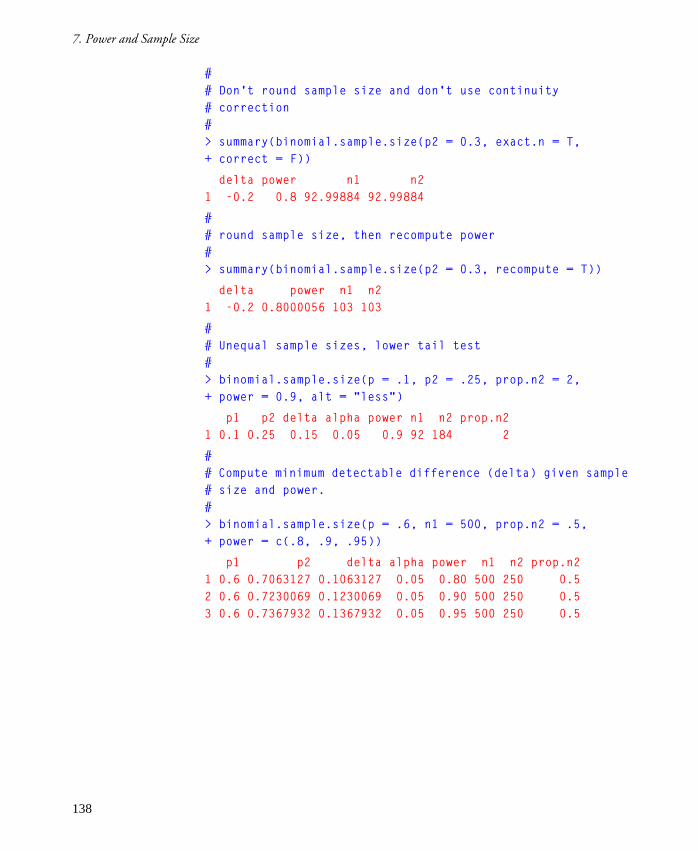
7. Power and Sample Size
#
# Don't round sample size and don't use continuity
# correction
#
> summary(binomial.sample.size(p2 = 0.3, exact.n = T,
+ correct = F))
delta power n1 n2
1 -0.2 0.8 92.99884 92.99884
#
# round sample size, then recompute power
#
> summary(binomial.sample.size(p2 = 0.3, recompute = T))
delta power n1 n2
1 -0.2 0.8000056 103 103
#
# Unequal sample sizes, lower tail test
#
> binomial.sample.size(p = .1, p2 = .25, prop.n2 = 2,
+ power = 0.9, alt = "less")
p1 p2 delta alpha power n1 n2 prop.n2
1 0.1 0.25 0.15 0.05 0.9 92 184 2
#
# Compute minimum detectable difference (delta) given sample
# size and power.
#
> binomial.sample.size(p = .6, n1 = 500, prop.n2 = .5,
+ power = c(.8, .9, .95))
p1 p2 delta alpha power n1 n2 prop.n2
1 0.6 0.7063127 0.1063127 0.05 0.80 500 250 0.5
2 0.6 0.7230069 0.1230069 0.05 0.90 500 250 0.5
3 0.6 0.7367932 0.1367932 0.05 0.95 500 250 0.5
138

References
#
# compute power
#
> binomial.sample.size(p = 0.3, p2 = seq(0.31, 0.35,
+ by=0.01), n1 = 1000, prop.n2 = 0.5)
p1 p2 delta alpha power n1 n2 prop.n2
1 0.3 0.31 0.01 0.05 0.06346465 1000 500 0.5
2 0.3 0.32 0.02 0.05 0.11442940 1000 500 0.5
3 0.3 0.33 0.03 0.05 0.20446778 1000 500 0.5
4 0.3 0.34 0.04 0.05 0.32982868 1000 500 0.5
5 0.3 0.35 0.05 0.05 0.47748335 1000 500 0.5
7.4 REFERENCES
Rosner, Bernard (1990). Fundamentals of Biostatistics (Third Edition).
PWS-Kent, Boston.
Fisher, Lloyd D. and Van Belle, Gerald (1993). Biostatistics. Wiley,
New York.
Fleiss, Joseph L. (1981). Statistical Methods for Rates and Proportions. Wiley,
New York.
139

7. Power and Sample Size
140

REGRESSION AND SMOOTHING
FOR CONTINUOUS RESPONSE
DATA8
8.1 Simple Least-Squares Regression 144
Diagnostic Plots for Linear Models 146
8.2 Multiple Regression 149
8.3 Adding and Dropping Terms From a Linear Model 152
8.4 Choosing the Best Model�Stepwise Selection 157
8.5 Updating Models 159
8.6 Weighted Regression 160
8.7 Prediction With the Model 163
8.8 Confidence Intervals 165
8.9 Polynomial Regression 168
8.10 Smoothing 172
Locally Weighted Regression Smoothing 173
Using the Super Smoother 174
Using the Kernel Smoother 176
Smoothing Splines 179
Comparing Smoothers 180
8.11 Additive Models 181
141

8. Regression and Smoothing for Continuous Response Data
142
8.12 More on Nonparametric Regression 187
Alternating Conditional Expectations 187
Additive and Variance Stabilizing Transformation 191
Projection Pursuit Regression 197
8.13 References 205

REGRESSION AND SMOOTHING FOR
CONTINUOUS RESPONSE DATA 8Regression is a tool for exploring relationships between variables. Linearregression explores relationships that are readily described by straight lines, ortheir generalization to many dimensions. A surprisingly large number ofproblems can be analyzed using the techniques of linear regression, and evenmore can be attacked by means of transformations of the original variablesthat result in linear relationships among the transformed variables. In recentyears, the techniques themselves have been extended through the addition ofrobust methods and generalizations of the classical linear regressiontechniques. These generalizations allow familiar problems in categorical dataanalysis such as logistic and Poisson regression to be subsumed under theheading of the generalized linear model (GLM), while still furthergeneralizations allow a predictor to be replaced by an arbitrary smoothfunction of the predictor in building a generalized additive model (GAM).
This chapter describes regression and smoothing in the case of a univariate,continuous response. We start with simple regression, that is, regression witha single predictor variable: fitting the model, examining the fitted models,and analyzing the residuals. We then examine multiple regression, varyingmodels by adding and dropping terms as appropriate. Again, we examine thefitted models and analyze the residuals. We then consider the special case ofweighted regression, which underlies many of the robust techniques andgeneralized regression methods.
One important reason for performing regression analysis is to get a modeluseful for prediction. The section Prediction With the Model describes howto use Axum to obtain predictions from your fitted model, and the sectionConfidence Intervals describes how to obtain pointwise and simultaneousconfidence intervals.
The classical linear regression techniques make several strong assumptionsabout the underlying data, and the data can fail to satisfy these assumptionsin different ways�for example, the regression line may be thrown off by oneor more outliers or the data may not be fitted well by any straight line. In thefirst case, we can bring robust regression methods into play; these minimize theeffects of outliers while retaining the basic form of the linear model.Conversely, the robust methods are often useful in identifying outliers. Wediscuss robust regression in detail in a later chapter.
143

8. Regression and Smoothing for Continuous Response Data
In the second case, we can expand our notion of the linear model, either byadding polynomial terms to our straight line model, or by replacing one ormore predictors by an arbitrary smooth function of the predictor, convertingthe classical linear model into a generalized additive model (GAM).
Scatterplot smoothers are useful tools for fitting arbitrary smooth functions toa scatter plot of data points. The smoother summarizes the trend of themeasured response as a function of the predictor variables. We describeseveral scatterplot smoothers available in Axum, and describe how thesmoothed values they return can be incorporated into additive models.
8.1 SIMPLE LEAST-SQUARES REGRESSIONSimple regression uses the method of least squares to fit a continuous,univariate response as a linear function of a single predictor variable. In themethod of least squares, we fit a line to the data so as to minimize the sum ofthe squared residuals. Given a set of n observations yi of the response variable
corresponding to a set of values xi of the predictor, and an arbitrary model
, the ith residual is defined as the difference between the ith
observation yi and the fitted value , that is .
To do simple regression with Axum, use the function lm (for linear model)with a simple formula linking your chosen response variable to the predictorvariable. In many cases, both the response and the predictor are componentsof a single data frame, which can be specified as the data argument to lm.For example, consider the air pollution data in the built-in data set air:
> air[,c(1,3)]
ozone temperature
1 3.448217 67
2 3.301927 72
3 2.289428 74
4 2.620741 62
5 2.843867 65
. . .
A scatter plot of the data is shown in figure 8.1. From the scatter plot, wehypothesize a linear relationship between temperature and ozoneconcentration. We choose ozone as the response, and temperature as thesingle predictor. The choice of response and predictor variables is driven bythe subject matter in which the data arise, rather than by statisticalconsiderations.
y f x( )=
yiˆ f xi( )= r i yi yi–=
144

Simple Least-Squares Regression
To fit the model, use lm as follows:
> ozone.lm <- lm(ozone ~ temperature, data = air)
The first argument, ozone ~ temperature, is the formula specifying thatthe variable ozone is modeled as a function of temperature. The secondargument specifies that the data for the linear model is contained in the dataframe air.
Use the summary function to obtain a summary of the fitted model:
> summary(ozone.lm)
Call: lm(formula = ozone ~ temperature)
Residuals:
Min 1Q Median 3Q Max
-1.49 -0.4258 0.02521 0.3636 2.044
Coefficients:
Value Std. Error t value Pr(>|t|)
(Intercept) -2.2260 0.4614 -4.8243 0.0000
temperature 0.0704 0.0059 11.9511 0.0000
Figure 8.1: Scatter plot of ozone against temperature.
••
•
••
•
•
••
••
•
•
•
•
•
•
•
•
•
•
•
•
••
•
•
••
•
•
• •
•
•
•
•
•
•
••
•
•
•
•
•
•
•
•
•
•
•
•
•
•
•
••
•
•
•
•
•
•
•
•
•
•
•
••
•
•
•
•
•
• •
•
•••
• •
•
•
•
•••
•
•
••
••
•
••
•
••
•
•
•
•
•
•••
temperature
ozon
e
60 70 80 90
12
34
5
145

8. Regression and Smoothing for Continuous Response Data
Residual standard error: 0.5885 on 109 degrees of freedom
Multiple R-Squared: 0.5672
F-statistic: 142.8 on 1 and 109 degrees of freedom, the p-value is 0
Correlation of Coefficients:
(Intercept)
temperature -0.9926
The Value column under Coefficients gives the coefficients of the linearmodel, allowing us to read off the estimated regression line as follows:
ozone = -2.2260 + 0.0704 × temperature
The column headed Std. Error gives the estimated standard error for eachcoefficient. The Multiple R-Squared term from the lm summary tells usthat the model explains about 57% of the variation in ozone. TheF-statistic is the ratio of the mean square of the regression to theestimated variance; if there is no relationship between temperature andozone, this ratio has an F distribution with 1 and 109 degrees of freedom.The ratio here is clearly significant, so the true slope of the regression line isprobably not 0.
Diagnostic
Plots for
Linear Models
Suppose we have the linear model defined as follows:
> ozone.lm <- lm(ozone ~ temperature, data=air)
How good is the fitted linear regression model? Is temperature an adequatepredictor of ozone concentration? Can we do better? Questions such as theseare essential any time you try to explain data with a statistical model.
It is not enough to fit a model; you must also assess how well that model fitsthe data, being ready to modify the model or abandon it altogether if it doesnot satisfactorily explain the data.
The simplest and most informative method for assessing the fit is to look atthe model graphically, using an assortment of plots that, taken together,reveal the strengths and weaknesses of the model. For example, a plot of theresponse against the fitted values gives a good idea of how well the model hascaptured the broad outlines of the data, while examining a plot of theresiduals against the fitted values often reveals unexplained structure left inthe residuals, which in a strong model should appear as nothing but noise.The default plotting method for lm objects provides these two plots, alongwith the following useful plots:
� Square root of absolute residuals against fitted values. This plot is usefulin identifying outliers and visualizing structure in the residuals.
146

Simple Least-Squares Regression
� Normal quantile plot of residuals. This plot provides a visual test ofthe assumption that the model�s errors are normally distributed. Ifthe ordered residuals cluster along the superimposed quantile-quantile line, you have strong evidence that the errors are indeednormal.
� Residual-Fit spread plot, or r-f plot. This plot compares the spread ofthe fitted values with the spread of the residuals. Since the model isan attempt to explain the variation in the data, you hope that thespread in the fitted values is much greater than that in the residuals.
� Cook�s distance plot. Cook�s distance is a measure of the influence ofindividual observations on the regression coefficients.
Calling plot as follows yields the six plots shown in figure 8.2:
> par(mfrow=c(2,3))
> plot(ozone.lm)
Figure 8.2: Default plots for lm objects.
••
•
• ••
• •• •
•
•
•
••
•
•••
•
••
•
•
••
•••
••
• •
•
••
••
• ••
••
•
••
• ••
•
••
•
••
•••
•
••
•••
••
•
•
•
• ••
••
•
•
•
•
•
••••••
•••••
• •••
••
••
•
•
•
• ••
•
• •
••
•
Fitted : temperature
Res
idua
ls
2.0 3.0 4.0
-10
12
45
2377
•
••
• ••
• •• •
•
•
•
•
•
•
••
•
•
•
•
•
•
•
•
••
•••
••
•
•
• ••
• ••
••
•
•• •
••
• •
••
•
•
•
••
•
•• •
•
•
•••
••
•••
••
•
•
• ••
•
•
•
•••
••
••
•
• •
••
•• •
•
•
•
•
• ••
•
••
••
•
Fitted : temperature
sqrt
(abs
(res
id(o
zone
.lm))
)
2.0 3.0 4.0
0.2
0.6
1.0
1.4
452377
• •
•• ••
••• •• •
•
•
•
•
•
••
••
•
•
• •
•
•••
••
• •
•
••
••
•••
•
•
•
••
••
•
•
••
•
••
•••
•
••
•••
••
•
•
•
•••
••
•
•
• ••
••••••
••
•••••
••
••
•
• ••
•••
•
••
•••
•
Fitted : temperature
ozon
e2.0 3.0 4.0
12
34
5
••
•
•••
••••
•
•
•
••
•
•• •
•
••
•
•
••
•••
••
••
•
••
••
••••
••
•
••
• ••
•
••
•
••
•••
•
••
••
•
••
•
•
•
• ••
••
•
•
•
•
•
• ••
•••
•••••
••• •
••
••
•
•
•
•••
•
• •
••
•
Quantiles of Standard Normal
Res
idua
ls
-2 -1 0 1 2
-10
12
45
2377
••••••••••••••••••••••••••••••••••••••••••••••••••••••
•••••••••••••••••••••••••••••
••••••••••••••••••••••••••••
Fitted Values
0.0 0.4 0.8
-10
12
••••••••••••••••
••••••••••••••••••
••••••••••••••••••••••••
••••••••••••••••••••••••••••••
••••••••••••••••••••••
•Residuals
0.0 0.4 0.8
-10
12
f-value
ozon
e
Index
Coo
k’s
Dis
tanc
e
0 20 40 60 80
0.0
0.04
17 7720
147

8. Regression and Smoothing for Continuous Response Data
The line y = is shown as a dashed line in the third plot (far right of top
row). In the case of simple regression, this line is visually equivalent to theregression line. The regression line appears to model the trend of the datareasonably well. The residuals plots (left and center, top row) show noobvious pattern, although five observations appear to be outliers. By default,as in figure 8.2, the three most extreme values are identified in each of theresiduals plots and the Cook�s distance plot. You can request a differentnumber of points by using the id.n argument in the call to plot; for thismodel, id.n=5 is a good choice.
Another useful diagnostic plot is the normal plot of residuals (left plot,bottom row). The normal plot gives no reason to doubt that the residuals arenormally distributed.
The r-f plot, on the other hand (middle plot, bottom row), shows a weaknessin this model; the spread of the residuals is actually greater than the spread inthe original data. However, if we ignore the five outlying residuals, theresiduals are more tightly bunched than the original data.
The Cook�s distance plot shows four or five heavily influential observations.As the regression line fits the data reasonably well, the regression issignificant, and the residuals appear normally distributed, we feel justified inusing the regression line as a way to estimate the ozone concentration for agiven temperature. One important issue remains�the regression lineexplains only 57% of the variation in the data. We may be able to dosomewhat better by considering the effect of other variables on the ozoneconcentration. See the section Multiple Regression for this further analysis.
At times, you are not interested in all of the plots created by the defaultplotting method. To view only those plots of interest to you, call plot withthe argument ask=T. This call brings up a menu listing the available plots:
> par(mfrow=c(1,1))
> plot(ozone.lm, id.n=5, ask=T)
Make a plot selection (or 0 to exit):
1: plot: All
2: plot: Residuals vs Fitted Values
3: plot: Sqrt of abs(Residuals) vs Fitted Values
4: plot: Response vs Fitted Values
5: plot: Normal QQplot of Residuals
6: plot: r-f spread plot
7: plot: Cook�s Distances
Selection:
Enter the number of the desired plot.
y
148

Multiple Regression
If you want to view all the plots, but want them all to appear in a fullgraphics window, do not set par(mfrow=c(2,3)) before calling plot, anddo not use the ask=T argument. Instead, before calling plot, callpar(ask=T). This tells Axum to prompt you before displaying eachadditional plot.
8.2 MULTIPLE REGRESSIONYou can construct linear models involving more than one predictor as easilyin Axum as models with a single predictor. In general, each predictorcontributes a single term in the model formula; a single term may contributemore than one coefficient to the fit.
For example, consider the built-in data sets stack.loss and stack.x.Together, these data sets contain information on ammonia loss in amanufacturing process. The stack.x data set is a matrix with three columnsrepresenting three predictors: air flow, water temperature, and acidconcentration. The stack.loss data set is a vector containing the response.To make our computations easier, combine these two data sets into a singledata frame, then attach the data frame:
> stack.df <- data.frame(stack.loss, stack.x)
> stack.df
stack.loss Air.Flow Water.Temp Acid.Conc.
1 42 80 27 89
2 37 80 27 88
3 37 75 25 90
. . .
> attach(stack.df)
For multivariate data, it is usually a good idea to view the data as a wholeusing the pairwise scatter plots generated by the pairs function:
> pairs(stack.df)
The resulting plot is shown in figure 8.3.
Call lm as follows to model stack.loss as a linear function of the threepredictors:
> stack.lm <- lm(stack.loss ~ Air.Flow + Water.Temp +
+ Acid.Conc.)
> summary(stack.lm)
149

8. Regression and Smoothing for Continuous Response Data
Call: lm(formula = stack.loss ~ Air.Flow + Water.Temp + Acid.Conc.)
Residuals:
Min 1Q Median 3Q Max
-7.238 -1.712 -0.4551 2.361 5.698
Figure 8.3: Pairwise scatter plots of stack loss data.
stack.loss
50 55 60 65 70 75 80
•
••
•
•••
•••••
••••
• •
•
••
•
• • ••
•••• •
•• • •
•
75 80 85 90
1020
3040
•
• •
•
• ••
•• ••• •
••• • •
• •
5055
6065
7075
80 ••
•
••••
•••••
••••
•
•
Air.Flow
•
•
•• • •
••• • •
• • •
•
•
••
•
• •
•• ••• •
••• • •
•
•
••
••
••••
•
••
••
•••• •
•
••
•••
•
••••
••• • •
Water.Temp
1820
2224
26
••
••
••
••
• ••
••
••• •
• • •
10 20 30 40
7580
8590 •
••
••
••
•
•
••
•
•
•
•
•
••
•
•••
•
•
•
•
•
••
•
•
•
•
•
••
•
•
18 20 22 24 26
••
•
•• •
•
•
•
••
•
•
•
•
•
•••
•
Acid.Conc.
150

Multiple Regression
Coefficients:
Value Std. Error t value Pr(>|t|)
(Intercept) -39.9197 11.8960 -3.3557 0.0038
Air.Flow 0.7156 0.1349 5.3066 0.0001
Water.Temp 1.2953 0.3680 3.5196 0.0026
Acid.Conc. -0.1521 0.1563 -0.9733 0.3440
Residual standard error: 3.243 on 17 degrees of freedom
Multiple R-Squared: 0.9136
F-statistic: 59.9 on 3 and 17 degrees of freedom, the p-value is 3.016e-09
Correlation of Coefficients:
(Intercept) Air.Flow Water.Temp
Air.Flow 0.1793
Water.Temp -0.1489 -0.7356
Acid.Conc. -0.9016 -0.3389 0.0002
When the response is the first variable in the data frame, as in stack.df,and the desired model includes all the variables in the data frame, the nameof the data frame itself can be supplied in place of the formula and dataarguments:
> lm(stack.df)
Call:
lm(formula = stack.df)
Coefficients:
(Intercept) Air.Flow Water.Temp Acid.Conc.
-39.91967 0.7156402 1.295286 -0.1521225
Degrees of freedom: 21 total; 17 residual
Residual standard error: 3.243364
We examine the default plots to assess the quality of the model (seefigure 8.4):
> par(mfrow=c(2,3))
> plot(stack.lm, ask=F)
Both the line y = and the residuals plots give support to the model. The
multiple R2 and F statistic also support the model. But would a simplermodel suffice?
y
151

8. Regression and Smoothing for Continuous Response Data
To find out, let�s return to the summary of the stack.lm model. From the tvalues, and the associated p-values, it appears that both Air.Flow andWater.Temp contribute significantly to the fit. But can we improve themodel by dropping the Acid.Conc. term? We explore this question furtherin section 8.3, Adding and Dropping Terms From a Linear Model.
8.3 ADDING AND DROPPING TERMS FROM A LINEAR MODELIn section 8.2, Multiple Regression, we fitted a linear model with threepredictors, of which only two appeared to be significant. Can we improve themodel stack.lm by dropping one or more terms?
The drop1 function takes a fitted model and returns an ANOVA tableshowing the effects of dropping in turn each term in the model:
Figure 8.4: Default plots of fitted model.
•
•
••
••••
•
•••
••
••
•••
•
•
Fitted : Air.Flow + Water.Temp + Acid.Conc
Res
idua
ls
10 20 30 40
-6-2
24
6
34
21
•
•
••
•
•••
•
•
••
•
•
•
••
••
•
•
Fitted : Air.Flow + Water.Temp + Acid.Conc
sqrt
(abs
(res
id(s
tack
.lm))
)
10 20 30 40
0.5
1.5
2.5
3421 •
••
•
•••••••• ••
•• •••
• •
Fitted : Air.Flow + Water.Temp + Acid.Concst
ack.
loss
10 20 30 40
1020
3040
•
•
••
•• •
••
•• •
••
••
•••
•
•
Quantiles of Standard Normal
Res
idua
ls
-2 -1 0 1 2
-6-2
24
6
34
21
•••••
••••••
•••••••
•
••Fitted Values
0.0 0.4 0.8
-10
010
20
•
•••••••••••
•••••••
••
Residuals
0.0 0.4 0.8
-10
010
20
f-value
stac
k.lo
ss
Index
Coo
k’s
Dis
tanc
e
5 10 15 20
0.0
0.4
41
21
152

Adding and Dropping Terms From a Linear Model
> drop1(stack.lm)
Single term deletions
Model:
stack.loss ~ Air.Flow + Water.Temp + Acid.Conc.
Df Sum of Sq RSS Cp
<none> 178.8300 262.9852
Air.Flow 1 296.2281 475.0580 538.1745
Water.Temp 1 130.3076 309.1376 372.2541
Acid.Conc. 1 9.9654 188.7953 251.9118
The columns of the returned value show the degrees of freedom for eachdeleted term, the sum of squares corresponding to the deleted term, theresidual sum of squares from the resulting model, and the Cp statistic for theterms in the reduced model.
The Cp statistic (actually, what is shown is the AIC statistic, the likelihoodversion of the Cp statistic�the two are related by the equation
) provides a convenient criterion for determining
whether a model is improved by dropping a term. If any term has a Cp
statistic lower than that of the current model (shown on the line labeled<none>), the term with the lowest Cp statistic is dropped. If the currentmodel has the lowest Cp statistic, the model is not improved by dropping anyterm. The regression literature discusses many other criteria for adding anddropping terms. See, for example, chapter 8 of Weisberg (1985).
In our example, the Cp statistic shown for Acid.Conc. is lower than that forthe current model. So it is probably worthwhile dropping that term from themodel:
> stack2.lm <- lm(stack.loss ~ Air.Flow + Water.Temp)
> stack2.lm
Call:
lm(formula = stack.loss ~ Air.Flow + Water.Temp)
Coefficients:
(Intercept) Air.Flow Water.Temp
-50.35884 0.6711544 1.295351
Degrees of freedom: 21 total; 18 residual
Residual standard error: 3.238615
AIC σ2
Cp n+( )=
153

8. Regression and Smoothing for Continuous Response Data
A look at the summary shows that we have retained virtually all theexplanatory power of the more complicated model:
> summary(stack2.lm)
Call: lm(formula = stack.loss ~ Air.Flow + Water.Temp)
Residuals:
Min 1Q Median 3Q Max
-7.529 -1.75 0.1894 2.116 5.659
Coefficients:
Value Std. Error t value Pr(>|t|)
(Intercept) -50.3588 5.1383 -9.8006 0.0000
Air.Flow 0.6712 0.1267 5.2976 0.0000
Water.Temp 1.2954 0.3675 3.5249 0.0024
Residual standard error: 3.239 on 18 degrees of freedom
Multiple R-Squared: 0.9088
F-statistic: 89.64 on 2 and 18 degrees of freedom, the p-value is 4.382e-10
Correlation of Coefficients:
(Intercept) Air.Flow
Air.Flow -0.3104
Water.Temp -0.3438 -0.7819
The residual standard error has fallen, from 3.243 to 3.239, while themultiple R2 has decreased only slightly from 0.9136 to 0.9088.
We create the default set of diagnostic plots as follows:
> par(mfrow=c(2,3))
> plot(stack2.lm, ask=F)
These plots, shown in figure 8.5, support the simplified model.
We turn next to the opposite problem�adding terms to an existing model.Our first linear model hypothesized a relationship between temperature andatmospheric ozone, based on a scatter plot showing an apparent linearrelationship between the two variables. The air data set containing the twovariables ozone and temperature also includes two other variables,radiation and wind. Pairwise scatter plots for all the variables can beconstructed using pairs as follows:
154

Adding and Dropping Terms From a Linear Model
> pairs(air)
The resulting plot is shown in figure 8.6. The plot in the top row, thirdcolumn of figure 8.6 corresponds to the scatter plot shown in figure 8.1.
From the pairwise plots, it appears that the ozone varies somewhat linearlywith each of the variables radiation, temperature, and wind, and thedependence on wind has a negative slope.
We can use the add1 function to add the terms wind and radiation inturn to our previously fitted model:
> ozone.add1 <- add1(ozone.lm, ~ temperature + wind + radiation)
> ozone.add1
Single term additions
Model:
ozone ~ temperature
Df Sum of Sq RSS Cp
<none> 37.74698 39.13219
wind 1 5.839621 31.90736 33.98517
radiation 1 3.839049 33.90793 35.98575
Figure 8.5: Diagnostic plots for simplified model.
•
•
••
•• ••
•
••
• •
•• • •
•
•
Fitted : Air.Flow + Water.Temp
Res
idua
ls
10 20 30
-8-4
02
46
34
21
•
•
••
•
• ••
•••
• ••
•• •
•
•
Fitted : Air.Flow + Water.Temp
sqrt
(abs
(res
id(s
tack
2.lm
)))
10 20 30
0.5
1.5
2.5
3421 •
••
•
• • ••••• • •
•• • •
• •
Fitted : Air.Flow + Water.Temp
stac
k.lo
ss
10 20 30
1020
3040
•
•
••
••••
•
• • •
••
•••••
•
•
Quantiles of Standard Normal
Res
idua
ls
-2 -1 0 1 2
-8-4
02
46
34
21
••••••
•••••
•••••••
•
••Fitted Values
0.0 0.4 0.8
-10
05
1020
•
••••••••
•••••••••
•••
Residuals
0.0 0.4 0.8
-10
05
1020
f-value
stac
k.lo
ss
Index
Coo
k’s
Dis
tanc
e
5 10 15 20
0.0
0.4
0.8
31
21
155

8. Regression and Smoothing for Continuous Response Data
The first argument to add1 is a fitted model object, the second a formulaspecifying the scope, that is, the possible choices of terms to be added to themodel. No response need be specified in the formula supplied; the responsemust be the same as that in the fitted model. The returned object is anANOVA table like that returned by drop1, showing the sum of squares dueto the added term, the residual sum of squares of the new model, and themodified Cp statistic for the terms in the augmented model. Each row of the
Figure 8.6: Pairwise scatter plots for ozone data.
ozone
0 50 150 250
••
••
••
•
•••
••
•
•
•
•
•
•
•
••
•
•
••
•
•
• •
•
•• •
•
•
•
•
•
••••
•
•
•
••
••
•
•
••
•
•
•
•••
•
••
•
••
•
•
•
•
•
••
•
•
•
•
•
••
•
•••••
•
••
••• •
•
••
••
•
••
•• •
••
•
•
•
•• •
• •
••
••
•
•• •
••
•
•
•
•
•
•
•
••
•
•
••
•
•
••
•
•• •
•
•
•
•
•
•••
•
•
•
••
••
•
•
••
•
•
•
•••
•
••
•
••
•
•
•
•
•
•••
•
•
•
•
• •
•
••••••
••
••••
•
••
••
•
••
•••
••
•
•
•
•••
5 10 15 20
12
34
5
• •
••
• •
•
•• •
••
•
•
•
•
•
•
•
••
•
•
••
•
•
• •
•
•••
•
•
•
•
•
••• •
•
•
•
••
••
•
•
••
•
•
•
•• •
•
••
•
••
•
•
•
•
•
••
•
•
•
•
•
• •
•
•••••
•
••
••••
•
••
••
•
••
•• •
••
•
•
•
•• •
050
150
250
•
••
• •
•
•
••
•
•
••
•
•
•
•
•
•
•
•
••
•
•
••
•
•
•
•
••
•••
•
•
• ••
•
•
•
•
•• •
••
•
•
•
• •
•
•••
•
•
•
••
••
•
•
••
•
•
•
•
•
••
••••
••
•• •
••
••••
••
•
•
•
••
•
•
•
•
•
•
••
••
•
•
radiation•
••
• •
•
•
••
•
•
••
•
•
•
•
•
•
•
•
••
•
•
••
•
•
•
•
••
•••
•
•
• ••
•
•
•
•
•••
••
•
•
•
• •
•
•••
•
•
•
•••
•
•
•
••
•
•
•
•
•
••
• •• •
•••••
••
•••
••
••
•
•
••
•
•
•
•
•
•
••
• •
•
••
••
••
•
•
••
•
•
••
•
•
•
•
•
•
•
•
••
•
•
••
•
•
•
•
••
•••
•
•
• ••
•
•
•
•
• ••
••
•
•
•
• •
•
•• •
•
•
•
••
••
•
•
••
•
•
•
•
•
••
• •• •
••
•• •
• •
•••
•••
•
•
•
• •
•
•
•
•
•
•
••
• •
•
•
•
••
••
••
••
•
•
••
•
•
••
•
• •
•
••
•
•
••
•
•
•
•
••
•••
••
••
•
•
•• •••
••
•
• ••
••
••
••• •
•• ••
••
••
•• ••
•
••
•
••
••
••• •
••
••••
•
• •
• •
•
•
•
•
•
•
•
•
•
•
•
• •
• •
••
••
••
••
•
•
••
•
•
••
•
• •
•
••
•
•
••
•
•
•
•
••
•••
• •
•••
•
•
•• • ••
••
•
••••
••
•••• •
••••
••
••
••• •
•
••
•
•••
•• •••
••
•••
•
•
••
• •
•
•
•
•
•
•
•
•
•
•
•
••
•
temperature
6070
8090
•
••
••
••
••
•
•
••
•
•
••
•
• •
•
••
•
•
••
•
•
•
•
••
• ••
• •
•••
•
•
••• ••
••
•
•••
••••
•• ••
• ••••
••
••
•• •
•
••
•
••
••••• •
••
•••
•
•
••
••
•
•
•
•
•
•
•
•
•
•
•
••
•
1 2 3 4 5
510
1520
••
••
•
•
•
•••
•• •
•
•••
•
•
••
•
••
•
•
•
•
•
•
•
••
•
••
•
•
•••
•
• ••
•
•
••
•
•• ••
•
•• ••
•
•
•
•
•
•
••••
••
• •
••
•
•
••
•
•• ••
••
•
•
••••
••
•
• •
•
•
• •
•
•
•••
•
•
•
•
•
••
••
•
•
•
• ••
•••
•
•••
•
•
••
•
••
•
•
•
•
•
•
•
••
•
••
•
•
•••
•
•••
•
•
••
•
••••
•
• •••
•
•
•
•
•
•
• •••
••
••
••
•
•
••
•
••••
••
•
•
••• •
• •
•
• •
•
•
• •
•
•
•••
•
•
•
•
•
60 70 80 90
• •
••
•
•
•
•••
•• •
•
•••
•
•
• •
•
••
•
•
•
•
•
•
•
••
•
••
•
•
•••
•
• ••
•
•
••
•
••••
•
••••
•
•
•
•
•
•
••••
••
••
••
•
•
••
•
••••
••
•
•
••••
••
•
••
•
•
••
•
•
•••
•
•
•
•
• wind
156

Choosing the Best Model�Stepwise Selection
ANOVA table represents the effects of a single term added to the base model.In general, it is worth adding a term if the Cp statistic for that term is lowestamong the rows in the table, including the base model term. In our example,we conclude that it is worthwhile adding the wind term.
Our choice of temperature as the original predictor in the model, however,was completely arbitrary. We can gain a truer picture of the effects of addingterms by starting from a simple intercept model:
> ozone0.lm <- lm(ozone ~ 1, data=air)
> ozone0.add1 <- add1(ozone0.lm, ~ temperature + wind +
+ radiation)
> ozone0.add1
Single term additions
Model:
ozone ~ 1
Df Sum of Sq RSS Cp
<none> 87.20876 88.79437
temperature 1 49.46178 37.74698 40.91821
wind 1 31.28305 55.92571 59.09694
radiation 1 15.53144 71.67732 74.84855
The obvious conclusion is that we should start with the temperature term,as we did originally.
8.4 CHOOSING THE BEST MODEL�STEPWISE SELECTIONAdding and dropping terms using add1 and drop1 is a useful method forselecting a model when only a few terms are involved, but it can quicklybecome tedious. The step function provides an automatic procedure forconducting stepwise model selection. Essentially what step does is automatethe selection process implied in section 8.3�that is, it calculates the Cp
statistics for the current model, as well as those for all reduced andaugmented models, then adds or drops the term that reduces Cp the most.The step function requires an initial model, often constructed explicitly asan intercept-only model, such as the ozone0.lm model constructed insection 8.3. Because step calculates augmented models, it requires a scopeargument, just like add1.
For example, suppose we want to find the �best� model involving the stackloss data, we could create an intercept-only model and then call step asfollows:
> stack0.lm <- lm(stack.loss ~ 1, data = stack.df)
> step(stack0.lm, ~ Air.Flow + Water.Temp + Acid.Conc.)
157

8. Regression and Smoothing for Continuous Response Data
Start: AIC= 2276.162
stack.loss ~ 1
Single term additions
Model:
stack.loss ~ 1
scale: 103.4619
Df Sum of Sq RSS Cp
<none> 2069.238 2276.162
Air.Flow 1 1750.122 319.116 732.964
Water.Temp 1 1586.087 483.151 896.998
Acid.Conc. 1 330.796 1738.442 2152.290
Step: AIC= 732.9637
stack.loss ~ Air.Flow
Single term deletions
Model:
stack.loss ~ Air.Flow
scale: 103.4619
Df Sum of Sq RSS Cp
<none> 319.116 732.964
Air.Flow 1 1750.122 2069.238 2276.162
Single term additions
Model:
stack.loss ~ Air.Flow
scale: 103.4619
158

Updating Models
Df Sum of Sq RSS Cp
<none> 319.1161 732.9637
Water.Temp 1 130.3208 188.7953 809.5668
Acid.Conc. 1 9.9785 309.1376 929.9090
Call:
lm(formula = stack.loss ~ Air.Flow, data = stack.df)
Coefficients:
(Intercept) Air.Flow
-44.13202 1.020309
Degrees of freedom: 21 total; 19 residual
Residual standard error (on weighted scale): 4.098242
The value returned by step is an object of class "lm", and the final resultappears in exactly the same form as the output of lm. However, by default,step displays the output of each step of the selection process. You can turnoff this display by calling step with the trace=F argument:
> step(stack0.lm, ~ Air.Flow + Water.Temp + Acid.Conc.,
+ trace=F)
Call:
lm(formula = stack.loss ~ Air.Flow, data = stack.df)
Coefficients:
(Intercept) Air.Flow
-44.13202 1.020309
Degrees of freedom: 21 total; 19 residual
Residual standard error (on weighted scale): 4.098242
8.5 UPDATING MODELSWe built our alternate model for the stack loss data by explicitly constructinga second call to lm. For models involving only one or two predictors, this isnot usually too burdensome. However, if you are looking at many differentcombinations of many different predictors, constructing the full callrepeatedly can be tedious.
The update function provides a convenient way for you to fit new modelsfrom old models, by specifying an updated formula or other arguments. Forexample, we could create the alternate model stack2.lm using update asfollows:
159

8. Regression and Smoothing for Continuous Response Data
> stack2a.lm <- update(stack.lm, .~. - Acid.Conc.,
+ data=stack.df)
> stack2a.lm
Call:
lm(formula = stack.loss ~ Air.Flow + Water.Temp, data
= stack.df)
Coefficients:
(Intercept) Air.Flow Water.Temp
-50.35884 0.6711544 1.295351
Degrees of freedom: 21 total; 18 residual
Residual standard error: 3.238615
The first argument to update is always a model object, and additionalarguments for lm are passed as necessary. The formula argument typicallymakes use of the �.� notation on either side of the �~�. The �.� indicates �asin previous model.� The �-� and �+� operators are used to delete or addterms. See chapter 2, Specifying Models in S-PLUS, for more information onformulas with update.
8.6 WEIGHTED REGRESSIONYou can supply weights in fitting any linear model; this can sometimesimprove the fit of models with repeated values in the predictor. Weightedregression is the appropriate method in those cases where it is known a priorithat not all observations contribute equally to the fit.
For example, a software company with a successful training departmentwanted to estimate the revenue to be generated by an expanded trainingschedule. For previous courses, the company had the data shown in table 8.1concerning the number of courses per month and revenue generated.
160

Weighted Regression
We create an Axum data frame from the data in table 8.1 as follows:
> ncourse <- c(2,2,2,3,3,3,3,4,4,4,5)
> revenue <- scan()
[1] 10030 7530 10801 18005 15455 14986 13926 16104
[9] 19166 18578 27596
> courserev <- data.frame(revenue, ncourse)
> courserev
Table 8.1: Revenue and courses per month.
Courses per month Revenue
2 10030
2 7530
2 10801
3 18005
3 15455
3 14986
3 13926
4 16104
4 19166
4 18578
5 27596
161

8. Regression and Smoothing for Continuous Response Data
revenue ncourse
1 10030 2
2 7530 2
3 10801 2
4 18005 3
5 15455 3
6 14986 3
7 13926 3
8 16104 4
9 19166 4
10 18578 4
11 27596 5
As a first look at the data, we fit a simple regression model as follows:
> course.lm <- lm(courserev)
> course.lm
Call:
lm(formula = courserev)
Coefficients:
(Intercept) ncourse
-650.3113 5123.726
Degrees of freedom: 11 total; 9 residual
Residual standard error: 2131.713
We then look at the default plots, shown in figure 8.7:
> par(mfrow=c(2,3))
> plot(course.lm)
Overall, the model seems to match the data reasonably well, but the residualslook to be increasing with the predictor. A weighted regression can help inthis case.
Weights are specified by supplying a non-negative vector as the weightsargument to lm. We weight with the number of observations for each valueof the predictor�this gives a higher weight to the lone observation for 5courses:
> course1.lm <- lm(revenue ~ ncourse, weights=c(1/3, 1/3,
+ 1/3, 1/4, 1/4, 1/4, 1/4, 1/3, 1/3, 1/3, 1))
> course1.lm
162

Prediction With the Model
Call:
lm(formula = revenue ~ ncourse, weights = c(1/3, 1/3,
1/3, 1/4, 1/4, 1/4, 1/4, 1/3, 1/3, 1/3, 1))
Coefficients:
(Intercept) ncourse
-2226.167 5678.333
Degrees of freedom: 11 total; 9 residual
Residual standard error (on weighted scale): 1297.942
The plots of the weighted regression show again a reasonable fit to the dataand a less obvious pattern to the residuals.
8.7 PREDICTION WITH THE MODELMuch of the value of a linear regression model is that, if it accurately modelsthe underlying phenomenon, it can provide reliable predictions about theresponse for a given value of the predictor. The predict function takes afitted model object and a data frame of new data, and returns a vector
Figure 8.7: Default diagnostic plots for unweighted course revenue model.
•
•
•
•
•••
•
••
•
Fitted : ncourse
Res
idua
ls
10000 15000 20000 25000
-400
00
2000 11
4
8•
•
•
•
•
•
•
•
•
•
•
Fitted : ncourse
sqrt
(abs
(res
id(c
ours
e.lm
)))
10000 15000 20000 25000
2030
4050
60
114
8
•••
••••
•••
•
Fitted : ncourse
reve
nue
10000 15000 20000 25000
1000
020
000
•
•
•
•
••
•
•
••
•
Quantiles of Standard Normal
Res
idua
ls
-1 0 1
-400
00
2000 11
4
8
• • •
• • • •
• • •
•Fitted Values
0.2 0.6
-500
00
5000
••
• • •• • • •
• •
Residuals
0.2 0.6
-500
00
5000
f-value
reve
nue
Index
Coo
k’s
Dis
tanc
e
2 4 6 8 10
0.0
0.4
0.8
28
11
163

8. Regression and Smoothing for Continuous Response Data
corresponding to the predicted response. The variable names in the new datamust correspond to those of the original predictors; the response may or maynot be present, but if present is ignored.
For example, suppose we want to predict the atmospheric ozoneconcentration from the following vector of temperatures:
> newtemp <- c(60, 62, 64, 66, 68, 70, 72)
We can obtain the desired predictions using predict as follows:
> predict(ozone.lm, data.frame(temperature=newtemp))
1 2 3 4 5 6
1.995822 2.136549 2.277276 2.418002 2.558729 2.699456
7
2.840183
The predicted values do not stand apart from the original observations.
You can use the se.fit argument to predict to obtain the standard errorof the fitted value at each of the new data points. When se.fit=T, theoutput of predict is a list, with a fit component containing the predictedvalues and an se.fit component containing the standard errors:
Figure 8.8: Diagnostic plots for weighted course revenue model.
•
•
•
•
•••
•
••
•
Fitted : ncourse
Res
idua
ls
10000 20000
-400
00
2000
10
4
8
•
••
•
•
•
•
•
••
•
Fitted : ncourse
sqrt
(abs
(res
id(c
ours
e1.lm
)))
10000 2000020
4060
10
4
8
•••
••••
•••
•
Fitted : ncourse
reve
nue
10000 20000
1000
020
000
•
•
•
•
•••
•
••
•
Quantiles of Standard Normal
Res
idua
ls
-1 0 1
-400
00
2000
10
4
8
• • •
• • • •
• • •
•Fitted Values
0.2 0.6
-500
00
5000
•
• • • •• • • • •
•
Residuals
0.2 0.6
-500
00
5000
f-value
reve
nue
Index
Coo
k’s
Dis
tanc
e
2 4 6 8 100
12
34
38
11
164

Confidence Intervals
> predict(ozone.lm, data.frame(temperature=newtemp), se.fit=T)
$fit:
1 2 3 4 5 6
1.995822 2.136549 2.277276 2.418002 2.558729 2.699456
7
2.840183
$se.fit:
1 2 3 4 5
0.1187178 0.1084689 0.09856156 0.08910993 0.08027508
6 7
0.07228355 0.06544499
$residual.scale:
[1] 0.5884748
$df:
[1] 109
You can use this output list to compute pointwise and simultaneousconfidence intervals for the fitted regression line. See section 8.8, ConfidenceIntervals, for details. See the predict help file for a description of theremaining components of the return list, $residual.scale and $df, aswell as a description of predict�s other arguments.
8.8 CONFIDENCE INTERVALSHow reliable is the estimate produced by a simple regression? Provided thestandard assumptions hold (that is, normal, identically distributed errorswith constant variance σ), we can construct confidence intervals for eachpoint on the fitted regression line based on the t distribution, andsimultaneous confidence bands for the fitted regression line using the Fdistribution.
In both cases, we need the standard error of the fitted value, se.fit, whichis computed as follows (Weisberg, 1985, p. 21):
se.fit σ 1n--- x x–( )2
xi x–( )2
i
∑---------------------------+
1
2---
=
165

8. Regression and Smoothing for Continuous Response Data
For a fitted object of class "lm", you can use the predict function as followsto calculate se.fit:
> predict(ozone.lm, se.fit=T)
$se.fit:
1 2 3 4
0.08460301 0.06544499 0.06015393 0.1084689
5
0.09377002 . . .
For any given point x in the predictor space, a 1 - α percent confidenceinterval for the fitted value corresponding to x is the set of values y such that
The pointwise function takes the output of predict (produced with these.fit=T flag), and returns a list containing three vectors: the vector oflower bounds, the fitted values, and the vector of upper bounds giving theconfidence intervals for the fitted values for the predictor:
> pointwise(predict(ozone.lm, se.fit=T))
$upper:
1 2 3 4 5 6
2.710169 3.011759 3.138615 2.42092 2.593475 2.250401
7
2.363895 . . .
$fit:
1 2 3 4 5 6
2.488366 2.840183 2.98091 2.136549 2.347639 1.925458
7
2.066185 . . .
$lower:
1 2 3 4 5 6
2.266563 2.668607 2.823205 1.852177 2.101803 1.600516
7
1.768476 . . .
The output from pointwise is suitable, for example, as input for theerror.bar function. It is tempting to believe that the curves resulting fromconnecting all the upper points and all the lower points would give aconfidence interval for the entire curve. This, however, is not the case; theresulting curve does not have the desired confidence level across its wholerange. What is required instead is a simultaneous confidence interval,
y t α n 2–,( ) se.fit y y t α n 2–,( ) se.fit×+< <×–
166

Confidence Intervals
obtained by replacing the t distribution with the F distribution. An Axumfunction for creating such simultaneous confidence intervals (and by defaultplotting the result) can be defined as follows:
"confint.lm"<-
function(object, alpha = 0.05, plot.it = T, ...)
{
f <- predict(object, se.fit = T)
p <- length(coef(object))
fit <- f$fit
adjust <- (p * qf(1 - alpha, p, length(fit) -
p))^0.5 * f$se.fit
lower <- fit - adjust
upper <- fit + adjust
if(plot.it) {
y <- fit + resid(object)
plot(fit, y)
abline(0, 1, lty = 2)
ord <- order(fit)
lines(fit[ord], lower[ord])
lines(fit[ord], upper[ord])
invisible(list(lower = lower, upper =
upper))
}
else list(lower = lower, upper = upper)
}
To see how it works, let�s create a plot of our first model of the ozone data:
> confint.lm(ozone.lm)
The resulting plot is shown in figure 8.9.
167

8. Regression and Smoothing for Continuous Response Data
8.9 POLYNOMIAL REGRESSION
Thus far in this chapter, we�ve dealt with data sets for which the graphicalevidence clearly indicated a linear relationship between the predictors and theresponse. For such data, the linear model is a natural and elegant choice,providing a simple and easily analyzed description of the data. But whatabout data that does not exhibit a linear dependence? For example, considerthe scatter plot shown in figure 8.10. Clearly, there is some functionalrelationship between the predictor E (for Ethanol) and the response NOx (forNitric Oxide), but just as clearly the relationship is not a straight line.
Figure 8.9: Simultaneous confidence intervals for ozone data.
••
•
••
•
•
••
••
•
•
•
•
•
•
•
•
•
•
•
•
••
•
•
••
•
•
• •
•
•
•
•
•
•
••
•
•
•
•
•
•
•
•
•
•
•
•
•
•
•
••
•
•
•
•
•
•
•
•
•
•
•
••
•
•
•
•
•
• •
•
•••
• •
•
•
•
•••
•
•
••
••
•
••
•
••
•
•
•
•
•
•••
fit
y
2.0 2.5 3.0 3.5 4.0 4.5
12
34
5
168

Polynomial Regression
How should we model such data? One approach is to add polynomial termsto the basic linear model, then use least-squares techniques as before. Theclassical linear model (with the intercept term represented as the coefficientof a dummy variable X0 of all 1s) is represented by an equation of the
following form:
where the predictors Xk enter the equation as linear terms. More generally,
classical linear regression techniques apply to any equation of the form
Figure 8.10: Scatter plot showing nonlinear dependence.
(8.1)
(8.2)
•
•
•
•
•
•
•
•
•
•
•
•••
•
•••
•
•
•
•
•
•
•
•
•
•
•
•
•
•
•
•
•
•
•
•
•
•
•
•
•
•
•
•
•
•
•
•
•
•
•
••
••
•
•
•
•
•
•
•
•
••
•
•
•
•
•
•
•
•
•
•
••
•
•
••••
••
•
E
NO
x
0.6 0.8 1.0 1.2
12
34
Y βk Xk ε+k 0=
n
∑=
Y βkZk ε+
k 0=
n
∑=
169

8. Regression and Smoothing for Continuous Response Data
where the Zk are new variables formed as combinations of the original
predictors. For example, consider a cubic polynomial relationship given bythe following equation:
Taking X = X1 = X2 = X3, we can convert this to the desired form by the
following assignments:
Once these assignments are made, the coefficients βk can be determined as
usual using the classical least-squares techniques.
To perform a polynomial regression in Axum, use lm together with the polyfunction. Use poly on the right hand side of the formula argument to lmto specify the independent variable and degree of the polynomial. Forexample, consider the following made-up data:
x <- runif(100, 0, 100)
y <- 50 - 43*x + 31*x^2 - 2*x^3 + rnorm(100)
We can fit this as a polynomial regression of degree 3 as follows:
> xylm <- lm(y ~ poly(x, 3))
> xylm
Call:
lm(formula = y ~ poly(x, 3))
Coefficients:
(Intercept) poly(x, 3)1 poly(x, 3)2 poly(x, 3)3
-329798.8 -3681644 -1738826 -333975.4
Degrees of freedom: 100 total; 96 residual
Residual standard error: 0.9463133
(8.3)Y βk Xk ε+
k 0=
3
∑=
X0 Z0=
X1 Z1=
X22 Z2=
X32 Z3=
170

Polynomial Regression
The coefficients appearing in the object xylm are the coefficients for theorthogonal form of the polynomial. To recover the simple polynomial form,use the function poly.transform:
> poly.transform(poly(x,3), coef(xylm))
x^0 x^1 x^2 x^3
49.9119 -43.01118 31.00052 -2.000005
These coefficients are very close to the exact values used to create y.
If the coefficients returned from a regression involving poly are so difficultto interpret, why not simply model the polynomial explicitly? That is, whynot use the formula y ~ x + x^2 + x^3 instead of the formula involvingpoly. In our example, there is little difference. However, in problemsinvolving polynomials of higher degree, severe numerical problems can arisein the model matrix. Using poly avoids these numerical problems, becausepoly uses an orthogonal set of basis functions to fit the various �powers� ofthe polynomial.
As a further example of the use of poly, let us consider the ethanol data wesaw at the beginning of this section. From figure 8.10, we are tempted by asimple quadratic polynomial. However, there is a definite upturn at each endof the data, so we are safer fitting a quartic polynomial, as follows:
> ethanol.poly <- lm(NOx ~ poly(E,degree=4))
> summary(ethanol.poly)
Call: lm(formula = NOx ~ poly(E, degree = 4))
Residuals:
Min 1Q Median 3Q Max
-0.8125 -0.1445 -0.02927 0.1607 1.017
Coefficients:
Value Std. Error t value
(Intercept) 1.9574 0.0393 49.8407
poly(E, degree = 4)1 -1.0747 0.3684 -2.9170
poly(E, degree = 4)2 -9.2606 0.3684 -25.1367
poly(E, degree = 4)3 -0.4879 0.3684 -1.3243
poly(E, degree = 4)4 3.6341 0.3684 9.8644
Pr(>|t|)
(Intercept) 0.0000
poly(E, degree = 4)1 0.0045
poly(E, degree = 4)2 0.0000
poly(E, degree = 4)3 0.1890
poly(E, degree = 4)4 0.0000
171

8. Regression and Smoothing for Continuous Response Data
Residual standard error: 0.3684 on 83 degrees of freedom
Multiple R-Squared: 0.8991
F-statistic: 184.9 on 4 and 83 degrees of freedom, the p-value is 0
Correlation of Coefficients:
(Intercept) poly(E, degree = 4)1
poly(E, degree = 4)1 0
poly(E, degree = 4)2 0 0
poly(E, degree = 4)3 0 0
poly(E, degree = 4)4 0 0
poly(E, degree = 4)2
poly(E, degree = 4)1
poly(E, degree = 4)2
poly(E, degree = 4)3 0
poly(E, degree = 4)4 0
poly(E, degree = 4)3
poly(E, degree = 4)1
poly(E, degree = 4)2
poly(E, degree = 4)3
poly(E, degree = 4)4 0
> poly.transform(poly(E,4), coef(ethanol.poly))
x^0 x^1 x^2 x^3 x^4
174.3601 -872.2071 1576.735 -1211.219 335.356
The summary clearly shows the significance of the 4th order term.
8.10 SMOOTHING
Polynomial regression can be useful in many situations. However, the choiceof terms is not always obvious, and small effects can be greatly magnified orlost completely by the wrong choice. Another approach to analyzingnonlinear data, attractive because it relies on the data to specify the form ofthe model, is to fit a curve to the data points locally, so that at any point thecurve at that point depends only on the observations at that point and somespecified neighboring points. Because such a fit produces an estimate of theresponse that is less variable than the original observed response, the result iscalled a smooth, and procedures for producing such fits are called scatterplotsmoothers. Axum offers a variety of scatterplot smoothers:
� loess.smooth a locally weighted regression smoother.
172

Smoothing
� smooth.spline a cubic smoothing spline, with local behaviorsimilar to that of kernel-type smoothers.
� ksmooth a kernel-type scatterplot smoother.
� supsmu a very fast variable span bivariate smoother.
Halfway between the global parameterization of a polynomial fit and thelocal, nonparametric fit provided by smoothers are the parametric fitsprovided by regression splines. Regression splines fit a continuous curve to thedata by piecing together polynomials fit to different portions of the data.Thus, like smoothers, they are local fits. Like polynomials, they provide aparametric fit. In Axum, regression splines can be used to specify the form ofa predictor in a linear or more general model, but are not intended for top-level use.
Locally
Weighted
Regression
Smoothing
In locally weighted regression smoothing, we build the smooth function s(x)pointwise as follows:
1. Take a point, say x0. Find the k nearest neighbors of x0, which
constitute a neighborhood N(x0). The number of neighbors k is
specified as a percentage of the total number of points. Thispercentage is called the span.
2. Calculate the largest distance between x0 and another point in the
neighborhood:
3. Assign weights to each point in N(x0) using the tri-cube weight
function:
where
4. Calculate the weighted least squares fit of y on the neighborhood
N(x0). Take the fitted value .
5. Repeat for each predictor value.
∆ x0( ) maxN x0( ) x0 x1–=
Wx0 x1–
∆ x0( )-------------------
W u( ) 1 u3–( )
3, for 0 u 1<≤
0 otherwise
=
y0 s x0( )=
173

8. Regression and Smoothing for Continuous Response Data
Use the loess.smooth function to calculate a locally weighted regressionsmooth. For example, suppose we want to smooth the ethanol data. Thefollowing expressions produce the plot shown in figure 8.11:
> plot(E,NOx)
> lines(loess.smooth(E,NOx))
The plot shown in figure 8.11 shows the default smoothing, which uses aspan of 2/3. For most uses, you will want to specify a smaller span, typicallyin the range of 0.3 to 0.5.
Using the
Super
Smoother
With loess, the span is constant over the entire range of predictor values.However, a constant value will not be optimal if either the error variance orthe curvature of the underlying function f varies over the range of x. Anincrease in the error variance requires an increase in the span whereas anincrease in the curvature of f requires a decrease. Local cross-validation avoidsthis problem by choosing a span for the predictor values xj based on only the
leave-one-out residuals whose predictor values xi are in the neighborhood of
xj. The super smoother, supsmu, uses local cross-validation to choose thespan. Thus, for one-predictor data, it can be a useful adjunct to loess.
Figure 8.11: Loess-smoothed ethanol data.
•
•
•
•
•
•
•
•
•
•
•
•••
•
•••
•
•
•
•
•
•
•
•
•
•
•
•
•
•
•
•
•
•
•
•
•
•
•
•
•
•
•
•
•
•
•
•
•
•
•
••
••
•
•
•
•
•
•
•
•
••
•
•
•
•
•
•
•
•
•
•
••
•
•
••••
••
•
E
NO
x
0.6 0.8 1.0 1.2
12
34
174

Smoothing
For example, figure 8.12 shows the result of super smoothing the responseNOx as a function of E in the ethanol data (dotted line) superimposed ona loess smooth. To create the plot, use the following commands:
> scatter.smooth(E,NOx, span=1/4)
> lines(supsmu(E,NOx), lty=2)
Local Cross-
Validation
Let s(x|k) denote the linear smoother value at x when span k is used. We wishto choose k = k(X) so as to minimize the mean squared error
where we are considering the joint random variable model for (X, Y ). Since
we would like to choose k = k(x) to minimize
.
However, we have only the data (xi, yi), i = 1, ..., n, and not the trueconditional distribution needed to compute EY|X=x, and so we cannot
Figure 8.12: Super Smoothed ethanol data (dotted line).
•
•
•
•
•
•
•
•
•
•
•
•••
•
•••
•
•
•
•
•
•
•
•
•
•
•
•
•
•
•
•
•
•
•
•
•
•
•
•
•
•
•
•
•
•
•
•
•
•
•
••
••
•
•
•
•
•
•
•
•
••
•
•
•
•
•
•
•
•
•
•
••
•
•
••••
••
•
E
NO
x
0.6 0.8 1.0 1.2
12
34
e2
k( ) EXY Y s X k( )–[ ]2=
EXY Y s X k( )–[ ]2EXEY X Y s X k( )–[ ]2=
ex2
k( ) EY X x Y s X k( )–[ ]2= =
EY X x Y s x k( )–[ ]2==
175

8. Regression and Smoothing for Continuous Response Data
calculate . Thus we resort to cross-validation and try to minimize thecross-validation estimate of :
.
Here s(i)(xi|k) is the �leave-one-out� smooth at xi , that is, s(i)(xi|k) is
constructed using all the data (xj, yj), j = 1, ..., n , except for (xi, yi), and then
the resultant local least squares line is evaluated at xi thereby giving s(i)(x|k).
The leave-one-out residuals
are easily obtained from the ordinary residuals
using the standard regression model relation
.
Here hii , i = 1, ..., n, are the diagonals of the so-called �hat� matrix, H = X
(XTX )-1XT , where, for the case at hand of local straight-line regression, X is a2-column matrix.
Using the
Kernel
Smoother
A kernel-type smoother is a type of local average smoother that, for each
target point xi in predictor space, calculates a weighted average of the
observations in a neighborhood of the target point:
where
.
ex2 k( )
ex2 k( )
eCV2
k( ) yi s i( ) xi k( )–[ ]2
i 1=
n
∑=
r i( ) k( ) yi s i( ) xi k( )–=
r i k( ) yi s xi k( )–=
r i( ) k( )r i k( )hii
-----------=
(8.4)
yi
yi wij yj
j 1=
n
∑=
wij Kxi xj–
b--------------
K
xi xj–
b--------------
Kxi xk–
b--------------
k 1=
n
∑-----------------------------------= =
176

Smoothing
are weights which sum to one:
.
The function K used to calculate the weights is called a kernel function,which typically has the following properties:
� (a)
� (b)
� (c)
Note that properties (a) and (b) are those of a probability density function.The parameter b is the bandwidth parameter, which determines how large aneighborhood of the target point is used to calculate the local average. A largebandwidth generates a smoother curve, while a small bandwidth generates awigglier curve. Hastie and Tibshirani (1990), point out that the choice ofbandwidth is much more important than the choice of kernel. To performkernel smoothing in Axum, use the ksmooth function. The kernels availablein ksmooth are shown in table 8.2.
Of the available kernels, the default "box" kernel gives the crudest smooth.For most data, the other three kernels yield virtually identical smooths. Werecommend "triangle" because it is the simplest and fastest to calculate.
The intuitive sense of the kernel estimate is clear: Values of yj such that xj
is close to xi get relatively heavy weights, while values of yj such that xj is far
from xi get small or zero weight. The bandwidth parameter b determines the
width of K(t/b), and hence controls the size of the region around xi for which
yj receives relatively large weights. Since bias increases and variance decreases
with increasing bandwidth b, selection of b is a compromise between biasand variance in order to achieve small mean squared error. In practice this isusually done by trial and error. For example, we can compute a kernelsmooth for the ethanol data as follows:
> plot(E,NOx)
> lines(ksmooth(E,NOx, kernel="triangle", bandwidth=.2))
> lines(ksmooth(E,NOx, kernel="triangle", bandwidth=.1),
+ lty=2)
wij 1=
j 1=
n
∑
K t( ) 0 for all t≥
K t( ) td∞–
∞∫ 1=
K t–( ) K t( ) for all t (symmetry)=
yi
177

8. Regression and Smoothing for Continuous Response Data
> legend(.54,4.1,c("bandwidth=.2", "bandwidth=.1"),
+ lty=c(1,2))
The resulting plot is shown in figure 8.13.
Table 8.2: Kernels available for ksmooth.
Kernel Explicit form
"box"
"triangle"1
"parzen"2
"normal"
In convolution form,
In convolution form,
The constants shown in the explicit forms above are used to scale theresulting kernel so that the upper and lower quartiles occur at ±.25. Also,the is taken to be 1 and the dependence of the kernel on the bandwidth issuppressed.
Kbox t( )1 , t 0.5≤0 , t 0.5>
=
Ktri t( )1 t C⁄ , – t
1C----≤
0 , t1C---->
=
Kpar t( )
k1 t2–( ) k2⁄ , t C1≤
t2 k3⁄( ) k4 t k5 , +– C1 t C2≤<
0 , C2 t<
=
Knor t( ) 1 2πk6⁄( ) exp t2 2k62⁄–( )=
Ktri t( ) Kbox * Kbox t( )=
Kpar t( ) Ktri * Kbox t( )=
178

Smoothing
Smoothing
Splines
A cubic smoothing spline behaves approximately like a kernel smoother, but it
arises as the function that minimizes the penalized residual sum of squares
given by
over all functions with continuous first and integrable second derivatives.The parameter λ is the smoothing parameter, corresponding to the span inloess or supsmu or the bandwidth in ksmooth.
To generate a cubic smoothing spline in Axum, use the functionsmooth.spline smooth to the input data:
> plot(E,NOx)
> lines(smooth.spline(E,NOx))
You can specify a different λ using the spar argument, although it is notintuitively obvious what a �good� choice of λ might be. When the data isnormalized to have a minimum of 0 and a maximum of 1, and when allweights are equal to 1, l=spar. More generally, the relationship is given by
Figure 8.13: Kernel smooth of ethanol data for two bandwidths.
•
•
•
•
•
•
•
•
•
•
•
•••
•
•••
•
•
•
•
•
•
•
•
•
•
•
•
•
•
•
•
•
•
•
•
•
•
•
•
•
•
•
•
•
•
•
•
•
•
•
••
••
•
•
•
•
•
•
•
•
••
•
•
•
•
•
•
•
•
•
•
••
•
•
••••
••
•
E
NO
x
0.6 0.8 1.0 1.2
12
34
bandwidth=.2bandwidth=.1
f
PRSS yi f xi( )–( )2
i 1=
n
∑ λ f″ t( )( )2td∫+=
179

8. Regression and Smoothing for Continuous Response Data
l=(max(x)-min(x))3·mean(w)·spar. You should either let Axum choose thesmoothing parameter, using either ordinary or generalized cross-validation,or supply an alternative argument, df, which specifies the degrees of freedomfor the smooth. For example, to add a smooth with approximately 5 degreesof freedom to our previous plot, use the following:
> lines(smooth.spline(E,NOx, df=5), lty=2)
The resulting plot is shown in figure 8.14.
Comparing
Smoothers
The choice of a smoother is somewhat subjective. All the smoothers discussedin this section can generate reasonably good smooths; you might select one oranother based on theoretical considerations or the ease with which one oranother of the smoothing criteria can be applied. For a direct comparision ofthese smoothers, consider the artificial data constructed as follows:
> set.seed(14) # set the seed to reproduce this example
> e <- rnorm(200)
> x <- runif(200)
> y <- sin(2*pi*(1-x)2)+x*e
Figure 8.14: Smoothing spline of ethanol data with cross-validation(solid line) and pre-specified degrees of freedom.
•
•
•
•
•
•
•
•
•
•
•
•••
•
•••
•
•
•
•
•
•
•
•
•
•
•
•
•
•
•
•
•
•
•
•
•
•
•
•
•
•
•
•
•
•
•
•
•
•
•
••
••
•
•
•
•
•
•
•
•
••
•
•
•
•
•
•
•
•
•
•
••
•
•
••••
••
•
E
NO
x
0.6 0.8 1.0 1.2
12
34
180

Additive Models
A �perfect� smooth would recapture the original signal, f(x) = sin(2π(1-x)2),exactly. The following commands sort the input and calculate the exactsmooth:
> sx <- sort(x)
> fx <- sin(2*pi*(1-sx)2)
The following commands create a scatter plot of the original data, thensuperimpose the exact smooth and smooths calculated using each of thesmoothers described in this chapter:
> plot(x,y)
> lines(sx,fx)
> lines(supsmu(x,y),lty=2)
> lines(ksmooth(x,y),lty=3)
> lines(smooth.spline(x,y),lty=4)
> lines(loess.smooth(x,y),lty=5)
> legend(0,2,c("perfect", "supsmu", "ksmooth",
+ "smooth.spline", "loess"), lty=1:5)
The resulting plot is shown in figure 8.15. This comparison is crude, at best,because by default each of the smoothers does a different amount ofsmoothing. A fairer comparison would adjust the smoothing parameters tobe roughly equivalent.
8.11 ADDITIVE MODELS
An additive model extends the notion of a linear model by allowing some orall linear functions of the predictors to be replaced by arbitrary smoothfunctions of the predictors. Thus, the standard linear model
is replaced by the additive model
.
The standard linear regression model is a simple case of an additive model.Because the forms of the fi are generally unknown, they are estimated using
some form of scatterplot smoother.
Y βiXi ε+
i 0=
n
∑=
Y α fi Xi( ) ε+
i 1=
n
∑+=
181

8. Regression and Smoothing for Continuous Response Data
To fit an additive model in Axum, use the gam function, where gam standsfor generalized additive model. You provide a formula which may containordinary linear terms as well as terms fit using any of the following:
� loess smoothers, using the lo function;
� smoothing spline smoothers, using the s function;
� natural cubic splines, using the ns function;
� B-splines, using the bs function;
� polynomials, using poly.
The three functions ns, bs, and poly result in parametric fits; additivemodels involving only such terms can be analyzed in the classical linearmodel framework. The lo and s functions introduce nonparametric fittinginto the model. For example, the following call takes the ethanol data andmodels the response NOx as a function of the loess-smoothed predictor E:
> attach(ethanol)
> ethanol.gam <- gam(NOx ~ lo(E, degree=2))
Figure 8.15: Comparison of Axum smoothers.
••
•
••
•
•
••
•
•
•
•
•
•
•
•
•
•• •
•
•
•
•
•
•
•
•
•
•
••
•
••
•
•
•
•
••
••
•
•
•
•
•
• ••
•
•
••
•
•
•
•
•
• •
•
•
• ••
•
••
•
•
•
•
•
•
•
•
•
•
•
••
•
•
•
•
•
•
•
•
••
•
••
•
•
•• •
•
•
•
•
•
•
•
•
•
•
••
•
•
•
•
•
•
•
•
•
•
•
•
•
•
••
• •
•
•
•
•
•
•
•
•
•
•••
•
•
•
• •
•
•
•
•
•
•
•
•
•
•
•
•
•
•
•
••
••
•
•
•
•
••
•
•
•
•
•
••
•
•
•
•
••
•
•
•
•
•
•
•
•
•
•
•
••
x
y
0.0 0.2 0.4 0.6 0.8 1.0
-2-1
01
2
perfectsupsmuksmoothsmooth.splineloess
182

Additive Models
> ethanol.gam
Call:
gam(formula = NOx ~ lo(E, degree = 2))
Degrees of Freedom: 88 total; 81.1184 Residual
Residual Deviance: 9.1378
In the call to lo, we specify that the smooth is to be locally quadratic byusing the argument degree = 2. For data that is less obviously nonlinear,we would probably be satisfied with the default, which is locally linear fitting.The printed gam object closely resembles a printed lm object from linearregression�the call producing the model is shown, followed by the degreesof freedom and the residual deviance which serves the same role as the residualsum of squares in the linear model. The deviance is a function of the log-likelihood function, which is related to the probability mass function f(yi; µi)
for the observation yi given µi. The log-likelihood for a sample of n
observations is defined as follows:
The deviance is then defined as
where m* maximizes the log-likelihood over m unconstrained, and φ is thedispersion parameter. For a continuous response with normal errors, as in themodels we�ve been considering in this chapter, the dispersion parameter isjust the variance σ2, and the deviance reduces to the residual sum of squares.As with the residual sum of squares, the deviance can be made arbitrarilysmall by choosing an interpolating solution. As in the linear model case,however, we generally have a desire to keep the model as simple as possible.In the linear case, we try to keep the number of parameters, that is, thequantities estimated by the model coefficients, to a minimum. Additivemodels are generally nonparametric, but we can define for nonparametricmodels an equivalent number of parameters, which we would also like to keepas small as possible.
The equivalent number of parameters for gam models is defined in terms ofdegrees of freedom, or df. In fitting a parametric model, one degree of freedomis required to estimate each parameter. For an additive model with parametricterms, one degree of freedom is required for each coefficient the term
l m; y( ) log f yi ; µi( )i 1=
n
∑=
D y; m( )
D y; m( )φ
-------------------- 2l m∗; y( ) 2l m; y( )–=
183

8. Regression and Smoothing for Continuous Response Data
contributes to the model. Thus, for example, consider a model with anintercept, one term fit as a cubic polynomial, and one term fit as a quadraticpolynomial. The intercept term contributes one coefficient and requires onedegree of freedom, the cubic polynomial contributes three coefficients andthus requires three degrees of freedom, and the quadratic polynomialcontributes two coefficients and requires two more degrees of freedom. Thus,the entire model has six parameters, and uses six degrees of freedom. Aminimum of six observations is required to fit such a model. Modelsinvolving smoothed terms use both parametric and nonparametric degrees offreedom�parametric degrees of freedom result from fitting a linear(parametric) component for each smooth term, while the nonparametricdegrees of freedom result from fitting the smooth after the linear part hasbeen removed. The difference between the number of observations and thedegrees of freedom required to fit the model is the residual degrees of freedom.Conversely, the difference between the number of observations and theresidual degrees of freedom is the degrees of freedom required to fit themodel, which is the equivalent number of parameters for the model.
The summary method for gam objects shows the residual degrees of freedom,the parametric and nonparametric degrees of freedom for each term in themodel, together with additional information:
> summary(ethanol.gam)
Call: gam(formula = NOx ~ lo(E, degree = 2))
Deviance Residuals:
Min 1Q Median 3Q Max
-0.6814987 -0.1882066 -0.01673293 0.1741648 0.8479226
(Dispersion Parameter for Gaussian family taken to be 0.1126477 )
Null Deviance: 111.6238 on 87 degrees of freedom
Residual Deviance: 9.137801 on 81.1184 degrees of freedom
Number of Local Scoring Iterations: 1
DF for Terms and F-values for Nonparametric Effects
Df Npar Df Npar F Pr(F)
(Intercept) 1
lo(E, degree = 2) 2 3.9 35.61398 1.110223e-16
184

Additive Models
The Deviance Residuals are, for Gaussian models, just the ordinary
residuals . The Null Deviance is the deviance of the model
consisting solely of the intercept term.
The ethanol data set contains a third variable, C, which measures thecompression ratio of the engine. Figure 8.16 shows pairwise scatter plots forthe three variables. Let�s incorporate C as a linear term in our additive model:
> attach(ethanol)
> ethanol2.gam <- gam(NOx ~ C + lo(E, degree = 2))
> ethanol2.gam
Call:
gam(formula = NOx ~ C + lo(E, degree = 2))
Degrees of Freedom: 88 total; 80.1184 Residual
Residual Deviance: 5.16751
Figure 8.16: Pairs plot of the ethanol data.
yi µi–
NOx
8 10 14 18
•
•
•
•
•
•
••
•
•
•
• • ••
•••
•
•
•
•
•
••
•
•
•
•
•
••
•
•
••
•
•
•
•
•
••
••
•
•
•
•
•
•
•
•
••
••
•
•
•
•
•
•
•
•
•••
••
•
•
•
•
•
•
•
• •
•
•
•• • •• •
•
12
34
•
•
•
•
•
•
••
•
•
•
••••
• ••
•
•
•
•
•
••
•
•
•
•
•
••
•
•
••
•
•
•
•
•
••
••
•
•
•
•
•
•
•
•
••
• •
•
•
•
•
•
•
•
•
•• •
••
•
•
•
•
•
•
•
••
•
•
••••••
•
810
1418
••• ••
•• •
•• ••
•
•
•
• •
• •
••••
• •
• •
• ••
• •• ••
• ••• •
•• ••
• •• •• ••
•
• •
••
• ••• • ••
•• •
••
•• •
• • •••
•••
•
••
••
•
•
• •
C •• •• •
• ••
• •• •
•
•
•
• •
••
• •• •
••
• •
• ••
•• •• •
••• ••
• •• •
• •• •• ••
•
••
••
• •• •• • •
• ••
• •
• ••
• • • • •
• ••
•
• •
••
•
•
• •
1 2 3 4
•
•
••
•
•
••
•
•
•
••
•• •
••
•
•
••
••
•
•
•
•
•
•
•
•
•
••
•
••
••
•
••
•
•••
••
••
•
••
•
••
••
•
•
••
•
•
••
•
•
•
•
••
•
•
•
•
••
•
•
•
•••••
•
•
•
••
•
•
••
•
•
•
• •
•• •
• •
•
•
••
•••
•
•
•
•
•
•
•
•
••
•
••
••
•
••
•
•••
••
••
•
••
•
••
••
•
•
••
•
•
••
•
•
•
•
••
•
•
•
•
••
•
•
•
• • • • •
•
0.6 0.8 1.0 1.2
0.6
0.8
1.0
1.2
E
185

8. Regression and Smoothing for Continuous Response Data
> summary(ethanol2.gam)
Call: gam(formula = NOx ~ C + lo(E, degree = 2))
Deviance Residuals:
Min 1Q Median 3Q Max
-0.6113908 -0.166044 0.0268504 0.1585614 0.4871313
(Dispersion Parameter for Gaussian family taken to be 0.0644985 )
Null Deviance: 111.6238 on 87 degrees of freedom
Residual Deviance: 5.167513 on 80.1184 degrees of freedom
Number of Local Scoring Iterations: 1
DF for Terms and F-values for Nonparametric Effects
Df Npar Df Npar F Pr(F)
(Intercept) 1
C 1
lo(E, degree = 2) 2 3.9 57.95895 0
We can use the anova function to compare this model with the simplermodel involving E only:
> anova(ethanol.gam, ethanol2.gam, test="F")
Analysis of Deviance Table
Response: NOx
Terms Resid. Df Resid. Dev Test Df
1 lo(E, degree = 2) 81.1184 9.137801
2 C + lo(E, degree = 2) 80.1184 5.167513 +C 1
Deviance F Value Pr(F)
1
2 3.970288 61.55632 1.607059e-11
The model involving C is clearly better, since the residual deviance is cutalmost in half by expending only one more degree of freedom.
Is the additive model sufficient? Additive models stumble when there areinteractions among the various terms. In the case of the ethanol data, thereis a significant interaction between C and E. In such cases, a full local
186

More on Nonparametric Regression
regression model, fit using the loess function, is often more satisfactory. Wediscuss the ethanol data more thoroughly in the chapter Local RegressionModels.
8.12 MORE ON NONPARAMETRIC REGRESSION
The additive models fitted by gam in the section Additive Models are simpleexamples of nonparametric regression. The machinery of generalized additivemodels, proposed by Hastie and Tibshirani (1990), is just one approach tosuch nonparametric models. Axum includes several other functions forperforming nonparametric regression, including the ace function, whichimplements the first proposed technique for nonparametric regression�alternating conditional expectations. Axum also includes AVAS (Additive andVAriance Stabilizing transformations) and projection pursuit regression. Thissection describes these varieties of nonparametric regression.
Alternating
Conditional
Expectations
Alternating conditional expectations or ace, is an intuitively appealingtechnique introduced by Breiman and Friedman (1985). The idea is to findnonlinear transformations θ(y), φ1(x1), φ2(x2),�, φp(xp) of the response y
and predictors x1, x2,�, xp, respectively, such that the additive model
is a good approximation for the data yi, xi1,�, xip, i = 1,�, n. Let yi, x1,
x2,�, xp be random variables with joint distribution F, and let expectations
be taken with respect to F. Consider the goodness-of-fit measure
(8.5)
(8.6)
θ y( ) φ1 x1( ) φ2 x2( ) … φp xp( ) ε+ + + +=
e2
e2 θ, φ1, ...,φp( )
E θ y( ) φk xk( )k 1=
p
∑–
2
Eθ2y( )
------------------------------------------------------= =
187

8. Regression and Smoothing for Continuous Response Data
The measure e2 is the fraction of variance not explained by regressing θ(y) on
φ(x1),�,φ(xp) . The data-based version of e2 is
where and the , estimates of θ and the φj, are standardized so that
and the have mean zero: and ,
k=1,�,p. For the usual linear regression case, where
and
with the least squares regression coefficients, we have
and the squared multiple correlation coefficient is given by .
The transformations , ,�, are chosen to maximize the correlation
between and . Although ace is a useful
exploratory tool for determining which of the response y and the predictors
(8.7)e2
θ yi( ) φk xik( )k 1=
p
∑–
2
i 1=
n
∑
θ2 yi( )i 1=
n
∑--------------------------------------------------------------=
θ φj θ yi( )
φj xij( ) θ yi( )i 1=
n
∑ 0= φk xik( )i 1=
n
∑ 0=
θ yi( ) yi y–=
φ1 xi1 x1
–( ) xi1 x1
–( )β1 ,…, φp xip xp
–( ) xip xp
–( )βp==
β1 ,…, βp
eLS2 RSS
SSY----------
yi y–( ) xik xk–( )βk
k 1=
p
∑–
2
i 1=
n
∑
yi y–( )2
i 1=
n
∑------------------------------------------------------------------------------≡=
R2 1 eLS2–=
θ φ1 φp
θ yi( ) φ xi1( ) … φ xip( )+ +
188

More on Nonparametric Regression
x1,�,xp are in need of nonlinear transformations and what type of
transformation is needed, it can produce anomalous results if errors ε and the
fail to satisfy the independence and normality assumptions.
To illustrate the use of ace, construct an artificial data set with additive errors
with the εi�s being N(0, 10) random variables (that is, normal random
variables with mean 0 and variance 10 ), independent of the xi�s, with the xi�s
being U(0, 2) random variables (that is, random variables uniformlydistributed on the interval from 0 to 2).
> set.seed(14) # set the seed to reproduce this example
> x <- 2*runif(200)
> e <- rnorm(200, 0, sqrt(10))
> y <- exp(1+2*x) + e
Now use ace:
> a <- ace(x,y)
Set graphics for 3 × 2 layout of plots:
> par(mfrow=c(3,2))
Make plots to do the following:
1. Examine original data;
2. Examine transformation of y ;
3. Examine transformation of x ;
4. Check linearity of the fitted model;
5. Check residuals versus the fit:
The following Axum commands provide the desired plots:
> plot(x, y, sub="Original Data")
> plot(x, a$tx, sub="Transformed x vs. x")
> plot(y, a$ty, sub="Transformed y vs. y")
> plot(a$tx, a$ty, sub="Transformed y vs.
+ Continue string: Transformed x")
> plot(a$tx, a$ty - a$tx, xlab="tx",
+ ylab="residuals", sub="Residuals vs. Fit")
φ1 xi( )
yi e1 2xi+ εi i , i= 1,…,200+=
189

8. Regression and Smoothing for Continuous Response Data
Figure 8.17: ace example with additive errors
•
•
•••
•
•
•
•
•
•
•
••
•••
•
••
•
••
• ••
•
•
•
•
••
•
•
•
•
•
•
•
••
•
•
• •
•
•
•
•
•
•
•
• •
•
•
•
•
•
•
•
•
•
••
•
••
•
••
•
•
•
•
• •
•
••
•
••
•
•••
•
•
•
•
•
•
•
•
•••
•
•
•
•
•
•
•
••
•
•
•
•
•
•
•
•
•
•
•••
•
•
•
•
•
•
•
•
•
•
•••
•
•
••
••
•
•
••
•
•
•
••
•
••
•
•
•
••
•
•
•
•
•
••
•
•
•
•
•
•
•
••
•
••
•
• •
•
•
•
•
•
•
•
••
•
• •
••
•
••
•
•
•
•
•
Original Datax
y
0.0 0.5 1.0 1.5 2.0
020
4060
8010
012
014
0
•
•
••
••
•
•
•
••
•
• •
••
•
•
••
•
••
•• •
•
•
•
•
••
•
•
•
•
•
•
•
•
•
•
•
• •
•
•
•
•
•
•
•
••
••
•
••
•
•
•
•
••
•
••
•
•
•
•
•
••
••
•
••
•
••
•
•••
•
•
•
•
•
•
•
•
•• •
•
•
•
•
•
•
•
••
•
•
•
•
• •
•
•
•
•
•••
•
•
•
•
•
•
•
•
•
•
•••
•
•
••• •
•
•
••
•
•
•
••
•
••
•
•
•
••
•
•
•
•
•
••
•
•
•
•
•
•
•
••
•
••
•
• •
•
•
•
•
••
•
• •
•
• •
• •
•
••
•
•
•
•
•
Transformed x vs. xx
a$tx
0.0 0.5 1.0 1.5 2.0
-10
12
•
•
•••
•
•
•
•
•
•
•
••
•••
•
• •
•
••
•••
•
•
•
•
••
•
•
•
•
•
•
•
••
•
•
••
•
•
•
•
•
•
•
••
••
•
•
•
•
•
•
•
••
•
••
•
••
•
•
•
•
••
•
• •
•
••
•
•••
•
•
•
•
•
•
•
•
•• •
•
•
•
•
•
•
•
••
•
•
•
•
••
•
•
•
•
•••
•
•
•
•
•
•
•
•
•
•
•••
•
•
••• •
•
•
••
•
•
•
••
•
••
•
•
•
••
•
•
•
•
•
• •
•
•
•
•
•
•
•
••
•
••
•
• •
•
•
•
•
•
•
•
••
•
••
• •
•
• ••
•
•
•
•
Transformed y vs. yy
a$ty
0 20 40 60 80 100 120 140
-10
12
•
•
•••
•
•
•
•
•
•
•
••
•••
•
• •
•
••
• ••
•
•
•
•
••
•
•
•
•
•
•
•
••
•
•
••
•
•
•
•
•
•
•
••
••
•
•
•
•
•
•
•
••
•
••
•
••
•
•
•
•
• •
•
• •
•
••
•
•••
•
•
•
•
•
•
•
•
•• •
•
•
•
•
•
•
•
••
•
•
•
•
••
•
•
•
•
•••
•
•
•
•
•
•
•
•
•
•
•••
•
•
••••
•
•
••
•
•
•
••
•
••
•
•
•
••
•
•
•
•
•
••
•
•
•
•
•
•
•
••
•
••
•
••
•
•
•
•
•
•
•
••
•
• •
••
•
• ••
•
•
•
•
Transformed y vs. Transformed xa$tx
a$ty
-1 0 1 2
-10
12
•
•
•
•
••
••
•
•
•
•
•
•
•
•• •
•
•
•
•
•
•
•
•
•
•
•
•
••
•
•
• ••
•
•
•
•
••
••
•
••
•
•
•
•
•
•
•
•
•
•
•
•
•
•
•
•
•
•
• •
•
•
•
•
•
•
•
•
•
••
••
••
•
•
••
•
•
•
•
•
•
•
•
•
••
•
•
•
•
•
•
•
•
•
•
•
•
•
•
•
••
•
•
•
•
• •
•
•
•
•
•
•
•
••
•
•
•
•
•
••
•
•
•
•••
•••
••
•
•
•
•
•
••
•
•
•
•
•
•
•
•••
••
•
•
•
•
••
•
•
•
••
•
••
•
•
•
•
•
•
•
•
•
•
•••
•
•
•
•
•
•
Residuals vs. Fita$tx
resi
dual
s
-1 0 1 2
-0.1
0.0
0.1
0.2
190

More on Nonparametric Regression
These plots are displayed in figure 8.17, where the transformed values
and are denoted by ty and tx, respectively. The estimated
transformation tx = seems close to exponential, and except for the small
bend at the lower left, the estimated transformation ty = seems quite
linear. The linearity of the plot of ty versus tx reveals that a good additivemodel of the type shown in equation (8.5) has been achieved. Furthermore,the error variance appears to be relatively constant, except at the very lefthand
end. The plot of residuals, versus the fit
gives a clearer confirmation of the behavior of the residuals� variance.
Additive and
Variance
Stabilizing
Transformation
The term �avas� stands for additivity and variance stabilizingtransformation. Like ace, avas tries to find transformations θ(y), φ1(x1),�,
φp(xp) such that
provides a good additive model approximation for the data yi, xi1,�, xip, i=1,
2,�,n. However, avas differs from ace in that it chooses θ(y) to achieve aspecial variance stabilizing feature. In particular the goal of avas is toestimate transformations θ, φ1,�, φp which have the properties
and
θ y( )
φ y( )
φ x( )
θ y( )
r i θ yi( ) φ xi( )–= tx φ xi( )=
(8.8)
(8.9)
(8.10)
θ y( ) φ1 x1( ) φ2 x2( ) … φp xp( ) ε+ + + +=
E θ y( ) x1 … xp, ,[ ] φi xi( )i 1=
p
∑=
var θ y( ) φi xi( )i 1=
p
∑ constant=
191

8. Regression and Smoothing for Continuous Response Data
Here E[z|w] is the conditional expectation of z given w. The additivitystructure 8.9 is the same as for ace, and correspondingly the φi�s are
calculated by the backfitting algorithm
cycling through k = 1, 2,�, p until convergence. The variance stabilizing
aspect comes from equation (8.9). As in the case of ace, estimates and
, k = 1, 2,�, p are computed to approximately satisfy equations 8.8
through 8.11, with the conditional expectations in 8.8 and 8.11 estimatedusing the super smoother scatterplot smoother (see supsmu functiondocumentation). The equality 8.9 is approximately achieved by estimatingthe classic stabilizing transformation.
To illustrate the use of avas, construct an artificial data set with additiveerrors
with the εi�s being N(0, 10) random variables (that is, normal random
variables with mean 0 and variance 10), independent of the xi�s, with the xi�s
being U(0, 2) random variables (that is, random variables uniformlydistributed on the interval from 0 to 2).
> set.seed(14) #set the seed to reproduce this example > x <- runif(200, 0, 2)
> e <- rnorm(200, 0, sqrt(10))
> y <- exp(1+2*x) + e
Now use avas:
> a <- avas(x, y)
Set graphics for a 3 × 2 layout of plots:
> par(mfrow=c(3,2))
Make plots to: (1) examine original data; (2) examine transformation of x;(3) examine transformation of y; (4) check linearity of the fitted model;(5) check residuals versus the fit:
> plot(x, y, sub="Original data")
> plot(x, a$tx, sub="Transformed x vs. x")
> plot(y, a$ty, sub="Transformed y vs. y")
> plot(a$tx, a$ty, sub="Transformed y vs. Transformed x")
(8.11)φk xk( ) E θ y( ) φi xi( ) xk
i k≠∑–=
θ yi( )
φj xik( )
yi e1 2xi+ εi i , i= 1, …, 200+=
192

More on Nonparametric Regression
> plot(a$tx, a$ty - a$tx, ylab="Residuals",
+ sub="Residuals vs. Fit")
These plots are displayed in figure 8.18 where the transformed values
and are denoted by ty and tx, respectively. The estimated
transformation tx = seems close to exponential, and the estimated
transformation ty = seems linear. The plot of ty versus tx reveals that a
linear additive model holds; that is, we have achieved a good additive
Figure 8.18: avas example with additive errors.
•
•
•••
•
•
•
•
•
•
•
••
•••
•
••
•
••
• ••
•
•
•
•
••
•
•
•
•
•
•
•
••
•
•
• •
•
•
•
•
•
•
•
• •
•
•
•
•
•
•
•
•
•
••
•
••
•
••
•
•
•
•
• •
•
••
•
••
•
•••
•
•
•
•
•
•
•
•
•••
•
•
•
•
•
•
•
••
•
•
•
•
•
•
•
•
•
•
•••
•
•
•
•
•
•
•
•
•
•
•
••
•
•
•
••
•
•
•
••
•
•
•
••
•
••
•
•
•
••
•
•
•
•
•
••
•
•
•
•
•
•
•
••
•
••
•
• •
•
•
•
•
•
•
•
••
•
• •
••
•
••
•
•
•
•
•
x
y
0.0 0.5 1.0 1.5 2.0
020
4060
8010
012
014
0
•
•
•
•
••
•
•
•
••
•
• •
••
•
•
••
•
••
•• •
•
•
•
•
••
•
•
•
•
•
•
•
•
•
•
•
••
•
•
•
•
•
•
•
••
••
•
••
•
•
•
•
••
•
••
•
••
•
•
••
••
•
••
•
••
•
•
••
•
•
•
•
•
•
•
•
•••
•
•
•
•
•
•
•
••
•
•
•
•
• •
•
•
•
•
•••
•
•
•
•
•
•
•
•
•
•
•
••
•
•
••• •
•
•
••
•
•
•
••
•
••
•
•
•
••
•
•
•
•
•
••
•
•
•
•
•
•
•
••
•
•
•
•
• •
•
•
•
•
••
•
• •
•
• •
••
•
•
••
•
•
•
•
x
a$tx
0.0 0.5 1.0 1.5 2.0
-10
12
•
•
•••
•
•
•
•
•
•
•
••
•••
•
••
•
••
•••
•
•
•
•
••
•
•
•
•
•
•
•
••
•
•
••
•
•
•
•
•
•
•
• •
•
••
•
•
•
•
•
•
••
•
••
•
••
•
•
•
•
••
•
••
•
••
•
•••
•
•
•
•
•
•
•
•
•••
•
•
•
•
•
•
•
••
•
•
•
•
•
•
•
•
•
•
•••
•
•
•
•
•
•
•
•
•
•
•••
•
•
••
••
•
•
••
•
•
•
••
•
••
•
•
•
••
•
•
•
•
•
• •
•
•
•
•
•
•
•
••
•
••
•
• •
•
•
•
•
•
•
•
••
•
••
••
•
••
•
•
•
•
•
y
a$ty
0 20 40 60 80 100 120 140
-10
12
•
•
•••
•
•
•
•
•
•
•
••
•••
•
••
•
••
• ••
•
•
•
•
••
•
•
•
•
•
•
•
••
•
•
• •
•
•
•
•
•
•
•
• •
•
••
•
•
•
•
•
•
••
•
••
•
••
•
•
•
•
• •
•
••
•
••
•
•••
•
•
•
•
•
•
•
•
•• •
•
•
•
•
•
•
•
••
•
•
•
•
•
•
•
•
•
•
•••
•
•
•
•
•
•
•
•
•
•
•••
•
•
••
••
•
•
••
•
•
•
• •
•
••
•
•
•
••
•
•
•
•
•
••
•
•
•
•
•
•
•
••
•
••
•
••
•
•
•
•
•
•
•
••
•
• •
••
•
••
•
•
•
•
•
a$tx
a$ty
-1 0 1 2
-10
12
•
••
•
•
••
•
•
•
•
•
•
•
•
•• ••
•
•
•
•
•
•
•
•
•
•
•
•• •
•
•••
•
•
•
•
•
•
•
•
••
•
•
•
•
•
•
••
••
•
•
•
•
•
•
•
•
•
• •
•
•
•
•
•
•
•
•
•
••
•
•
•
•
•
•
••
•
•
•
•
•
•
•
•
•
••
•
•
•
•
•
•
•
•
•
•
•
•
••
•
•
•
•
••
••
•
••
•
•
• •
•
••
•
•
•
•
•
•
•
•
• •
•
••
•
•
•
• •
•
••
•
•
••
•
•
•
•
•
•
•
•
•
•
••
•
•
••
• •
•
•
•
•
• •
••
•
•
•
•
•
•
•
•
•
••
•
•
•
•
•
•
•
•
a$tx
Res
idua
ls
-1 0 1 2
-0.2
-0.1
0.0
0.1
0.2
θ y( )
φ x( )
φ x( )
θ y( )
193

8. Regression and Smoothing for Continuous Response Data
approximation of the type 8.8. In this plot the error variance appears to be
relatively constant. The plot of residuals, ri = , versus the fit
tx = gives further confirmation of this.
Key Properties � Suppose that the true additive model is
with ε independent of x1, x2, ..., xp, and var(ε ) = constant. Then the
iterative avas algorithm for 8.9 � 8.11, described below for the data
versions of 8.9 � 8.11, yields a sequence of transformations ,
, ..., which converge to the true transformation , ,
..., , as the number of iterations j tends to infinity.
Correspondingly, the data-based version of this iteration yields a
sequence of transformations , , ..., , which, at
convergence, provide estimates , , ..., , of the true model
transformations , , ..., .
� avas appears not to suffer from some of the anomalies of ace, e.g.,not finding good estimates of a true additive model (equation 8.12)when normality of ε and joint normality of φ1(x1), �, φp(xp) fail to
hold. See the example below.
� avas is a generalization of the Box and Cox (1964) maximum-likelihood procedure for choosing power transformation yλ of theresponse. The function avas also generalizes the Box and Tidwell(1962) procedure for choosing transformations of the carriers x1, x2,
..., xp, and is much more convenient than the Box-Tidwell
procedure. See also Weisberg (1985).
� is a monotone transformation, since it is the integral of a
nonnegative function (see Further Details, below). This is important
if one wants to predict y by inverting : monotone transformations
θ yi( ) φ xi( )–
φ xi( )
(8.12)θ0y( ) φi
0xi( )
i 1=
p
∑ ε+=
θ j( )
φ1j( ) φp
j( ) θ0 φ10
φp0
θj( )
φ1j( )
φpj( )
θ φ1 φp
θ0 φ10 φp
0
θ y( )
θ
194

More on Nonparametric Regression
are invertible, and hence we can predict y with
. This predictor has no particular optimality
property, but is simply one straightforward way to get a prediction ofy once an avas model has been fit.
Further Details Let
where is an arbitrary transformation of y, will be the �previous�
estimate of θ(y) in the overall iterative procedure described below. Given thevariance function v(u), it is known that
will be constant if g is computed according to the rule
for an appropriate constant c. See Box and Cox (1964).
The detailed steps in the population version of the avas algorithm are asfollows:
1. Initialize:
Set and backfit on x1, ..., xp to get
, ..., . (See description of ace for details of �backfitting�.)
y θG1– φi xi( )
i 1=
p
∑=
(8.13)
(8.14)
v u( ) VAR θ y( ) φi xi( ) u=i 1=
p
∑=
θ y( ) θ y( )
VAR g θ y( )( ) φi xi( ) u=i 1=
p
∑
g t( )ud
v1 2⁄
u( )-----------------
c
t
∫=
θ y( ) y Ey–( ) VAR1 2⁄y( )⁄=
φ1 φp
195

8. Regression and Smoothing for Continuous Response Data
2. Get new transformation of y :a) Compute variance function
b) Compute variance stabilizing transformation
c) Set and standardize
3. Get new �s:
Backfit on x1, x2, �, xp to obtain new estimates , ...,
.
4. Iterate steps 2 and 3 until
doesn�t change.
Of course the above algorithm is actually carried out using the sample of datayi, xi1, ..., xip, i = 1, ..., n, with expectations replaced by sample averages,
conditional expectations replaced by scatterplot smoothing techniques andVAR�s replaced by sample variances.
In particular, super smoother is used in the backfitting step to obtain
, ..., , i = 1, ..., n. An estimate of v(u) is obtained as
follows: First the scatter plot of versus
(8.15)
v u( ) VAR θ y( ) φi xi( ) u=i 1=
p
∑=
g t( )ud
v1 2⁄
u( )-----------------
c
t
∫=
θ y( ) g θ y( )( )–
θ y( ) θ y( ) Eθ y( )–
VAR1 2⁄ θ y( )
--------------------------------–
φi
θ y( ) φ1
φp
R2 1 e
2– 1 E θ y( ) φi xi( )i 1=
p
∑–
2
–= =
φ1 xi1( ) φp xip( ) v u( )
logr i2 log θ yi( ) φj xij( )
j 1=
p
∑–
2
=
196

More on Nonparametric Regression
is smoothed using a running straight lines smoother.
Then the result is exponentiated. This gives an estimate , and
is truncated below at 10-10 to insure positivity and avoid dividing by zero inthe integral 8.14. The integration in equation 8.14 is carried out using atrapezoidal rule.
Projection
Pursuit
Regression
The basic idea behind projection pursuit regression, ppreg, is as follows. Lety and x = (x1, x2, ..., xp)
T denote the response and explanatory vector,
respectively. Suppose you have observations yi and corresponding predictors
xi = (xi1, xi2, ..., xip)T, i = 1, 2, ..., n. Let a1, a2 , ..., denote p-dimensional unit
vectors, as �direction� vectors, and let . The ppreg function
allows you to find M = M0, direction vectors a1, a2, ..., and good
nonlinear transformations φ1, φ2, ..., such that
provides a �good� model for the data yi, xi, i = 1, 2, ..., n . The �projection�
part of the term projection pursuit regression indicates that the carrier vector
x is projected onto the direction vectors a1, a2, ..., to get the lengths aTx,
i = 1, ..., n of the projections, and the �pursuit� part indicates that anoptimization technique is used to find �good� direction vectors a1, a2, ...,
.
More formally, y and x are presumed to satisfy the conditional expectationmodel
ui φj xij( )j 1=
p
∑=
v u( ) 0≥ v u( )
(8.16)
(8.17)
y1n--- yi
i 1=
n
∑=
aM0
φM0
y y βmφm amT x( )
m 1=
M0
∑+≈
aM0
aM0
E y x1, x2, ..., xp[ ] µy βmφm amT x( )
m 1=
M0
∑+=
197

8. Regression and Smoothing for Continuous Response Data
where µy = E(y), and the φm have been standardized to have mean zero and
unity variance:
The observations yi, xi = (xi1, ..., xip)T, i = 1, ..., n , are assumed to be
independent and identically distributed random variables like y and x, i.e.,they satisfy the model in equation 8.17.
The true model parameters βm, φm, am, m = 1, ..., M0 in equation 8.17
minimize the mean squared error
over all possible βm, φm, and am.
Equation 8.17 includes the additive ace models under the restriction θ(y) =y. This occurs when M0 = p and a1 = (1, 0, ..., 0)T, a2 = (0, 1, 0, ..., 0) T, ap = (0,
0, ..., 0, 1)T, and the βm�s are absorbed into the φm�s. Furthermore, the ordinary
linear model is obtained when M0 = 1, assuming the predictors x are
independent with mean 0 and variance 1. Then
, φ1(t) = t, and ,
where the bj are the regression coefficients.
The projection pursuit model in equation 8.17 includes the possibility ofhaving interactions between the explanatory variables. For example, supposethat
This is described by 8.17 with µy = 0, M0 = 2, , ,
, φ1(t) = t2, and φ2(t) = -t2. For then
m = 1, ..., M0. (8.18)Eφm amT x( ) 0,= Eφm
2 amT x( ) 1,=
(8.19)
E[y|x1, x2] = x1x2. (8.20)
E y µy– βmφm amT x( )
m 1=
M0
∑–
2
aTb1, ..., bp( ) b1
2 + … + bp2⁄= β1 b1
2 + … + bp2=
β1 β214---= = a1
T 1 1,( )=
a2T 1 1–,( )=
φ1 a1Tx( ) x1 x2+( )2
x12 2x1x2 x2
2+ += =
φ2 a2Tx( ) x1 x2–( )2– x– 1
2 2x1x2 x22–+= =
198

More on Nonparametric Regression
so that
.
Neither ace nor avas is able to model interactions. It is this ability to pickup interactions that led to the invention of projection pursuit regression byFriedman and Stuetzle (1981), and it is what makes ppreg a usefulcomplement to ace and avas.
The two variable interactions shown above can be used to illustrate theppreg function. The two predictors, x1 and x2 are generated as uniform
random variates on the interval - 1 to 1. The response, y, is the product of x1
and x2 plus a normal error with mean zero and variance 0.04.
> set.seed(14) #set the seed to reproduce this example
> x1 <- runif(400, -1, 1)
> x2 <- runif(400, -1, 1)
> eps <- rnorm(400, 0, .2)
> y <- x1*x2+eps
> x <- cbind(x1, x2)
Now run the projection pursuit regression with max.term set at 3,min.term set at 2 and with the residuals returned in the ypred component(the default if xpred is omitted).
> p <- ppreg(x, y, 2, 3)
Make plots (shown in figure 8.19) to examine the results of the regression.
> par(mfrow=c(3, 2))
> plot(x1, y, sub="Y vs X1")
> plot(x2, y, sub="Y vs X2")
> plot(p$z[,1], p$zhat[,1], sub="1st Term:
Continue string: Smooth vs Projection Values z1")
> plot(p$z[,2], p$zhat[,2], sub="2nd Term:
Continue string: Smooth vs Projection Values z2")
> plot(y-p$ypred, y, sub="Response vs Fit")
> plot(y-p$ypred, p$ypred, sub="Residuals vs Fit")
The first two plots show the response plotted against each of the predictors. Itis difficult to hypothesize a function form for the relationship when lookingat these plots. The next two plots show the resulting smooth functions fromthe regression plotted against their respective projection of the carriervariables. Both the plots have a quadratic shape with one being positive andthe other negative, the expected result for this type of interaction function.
βmφm aTx( )m 1=
2
∑ x1x2=
199

8. Regression and Smoothing for Continuous Response Data
The fifth plot shows clearly a linear relationship between the response andthe fitted values. The residuals shown in the last plot do not display anyunusual structure.
Figure 8.19: Projection pursuit example.
••
•
•
•
•
•
•
•
•
• •
•
•
•
•
•
•
••
•
•
••
•
••
•
•
•
•
•
•
•
•
•
•
•
•
•
•
•
••
•
•
••
•
•
•
•
•
•
•
•
•
••
••
••
•
••
•
•
•
•
••
•
••
•
•
•
••
•
•
••
•
•
•
•
•
•
•
•
•
•
•
•
•
•
••
•
•
•
•
• ••
••
••
•
•
••
•
•
•
•
•
•
•
•
•
•
•
•
•
•
•
•
• •
•
•
•
•
•
•
••
•
•
•
•
•
•
•
•
•
•
•
•
•
•
•
•
•
•
•
•
•
• •
•
•
•
•
•
••
•
•
•
•••
•
•• •
•
•
•
•
•
••
•
•
•
•
•
•
• ••
•
•
•
•
•
•
•
•
•
•
•
•
•
•
••
•
•
•
•
•
•
•
•
•
•
•
•
•
•
•
•
•
•
•
•
•• •• •
•
•
•
•
•
•
•
••
•
•
•
•
••
•
•
•
•
•
••
••
•
••••
•
•
•
•
•
•
•
••
••
•
•
•
••
••
•
••
••
•
• •
• •
•
•
•
•
•
•
•
•
•
•••
•
••
•
••
•
•
•
•••
•
•
•
•
•
•
••
•
•
••
•
•
•
•
•
•
••
•
•
•
•
•
•
•
•
•
•
•
•
• •
•
•
•
• ••
•
•• •
••
••
•
••
•
••
•
••
•••
••
•
•
•
•
•
•
• ••
•
•
•
•
•
•
•
•
•
•
Y vs X1x1
y
-1.0 -0.5 0.0 0.5 1.0
-1.0
-0.5
0.0
0.5
1.0
••
•
•
•
•
•
•
•
•
• •
•
•
•
•
•
•
••
•
•
••
•
••
•
•
•
•
•
•
•
•
•
•
•
•
•
•
•
••
•
•
••
•
•
•
•
•
•
•
•
•
••
••
••
•
••
•
•
•
•
••
•
••
•
•
•
••
•
•
• •
•
•
•
•
•
•
•
•
•
•
•
•
•
•
••
•
•
•
•
• ••
••
••
•
•
• •
•
•
•
•
•
•
•
•
•
•
•
•
•
•
•
•
••
•
•
•
•
•
•
••
•
•
•
•
•
•
•
•
•
•
•
•
•
•
•
•
•
•
•
•
•
••
•
•
•
•
•
••
•
•
•
• ••
•
•••
•
•
•
•
•
••
•
•
•
•
•
•
• ••
•
•
•
•
•
•
•
•
•
•
•
•
•
•
••
•
•
•
•
•
•
•
•
•
•
•
•
•
•
•
•
•
•
•
•
• • •••
•
•
•
•
•
•
•
••
•
•
•
•
••
•
•
•
•
•
••
••
•
•• ••
•
•
•
•
•
•
•
••
••
•
•
•
••
••
•
••
••
•
• •
••
•
•
•
•
•
•
•
•
•
• ••
•
••
•
••
•
•
•
•• •
•
•
•
•
•
•
••
•
•
••
•
•
•
•
•
•
••
•
•
•
•
•
•
•
•
•
•
•
•
••
•
•
•
•••
•
•• •
••
••
•
••
•
••
•
••
•••
••
•
•
•
•
•
•
• ••
•
•
•
•
•
•
•
•
•
•
Y vs X2x2
y
-1.0 -0.5 0.0 0.5 1.0
-1.0
-0.5
0.0
0.5
1.0
••••••••
••••••••••••••••••••••
•••••••••••••••••••••••
••••••••••••••••••••••••••
••••••••••••••••••••••••••••
••••••••••••••••••••••••••••••••••••
•••••••••••••••••••••••••••••••••••••••••••••••••••••••••••••••••••••••••••••••••••••••••••••••••••••••••••••••••••••••••••••••••••••••••••••••••••••••••••••••••••••••••••••••••••••••••••••••••••••••••••••••••••••••••••
••••••••••••••••••••
•••••••••••••
••••
•
1st Term:Smooth vs Projection Values z1
p$z[, 1]
p$
zha
t[,
1]
-1.0 -0.5 0.0 0.5 1.0
-4-3
-2-1
01
••••••••••••
•••••
••••••••••
•••••••••••••••••••••••••••••••••••••••••••••••••••••••••••••••••••••••••••••••••••••••••••••••••••••••••••••••••••••••••••••••••••••••••••••••••••••••••••••••••••••••••••••••••••••••••••••••••••••••••••••••••••••••••••••••••••••••••••••
•••••••••••••••••••••••••••
••••••••••••••••••••••••••
•••••••••••••••••••
•••••••••••••
•••••••••••••••••••••••••••••••••
•••••••••
••••••••
•
2nd Term:Smooth vs Projection Values z2
p$z[, 2]
p$
zha
t[,
2]
-1.0 -0.5 0.0 0.5 1.0
-10
12
3
••
•
•
•
•
•
•
•
•
• •
•
•
•
•
•
•
••
•
•
••
•
••
•
•
•
•
•
•
•
•
•
•
•
•
•
•
•
• •
•
•
••
•
•
•
•
•
•
•
•
•
••
••
••
•
••
•
•
•
•
••
•
••
•
•
•
••
•
•
• •
•
•
•
•
•
•
•
•
•
•
•
•
•
•
••
•
•
•
•
•••
••
••
•
•
••
•
•
•
•
•
•
•
•
•
•
•
•
•
•
•
•
••
•
•
•
•
•
•
••
•
•
•
•
•
•
•
•
•
•
•
•
•
•
•
•
•
•
•
•
•
• •
•
•
•
•
•
• •
•
•
•
•••
•
•••
•
•
•
•
•
••
•
•
•
•
•
•
• ••
•
•
•
•
•
•
•
•
•
•
•
•
•
•
••
•
•
•
•
•
•
•
•
•
•
•
•
•
•
•
•
•
•
•
•
•• •• •
•
•
•
•
•
•
•
••
•
•
•
•
••
•
•
•
•
•
••
••
•
•• • •
•
•
•
•
•
•
•
••
••
•
•
•
••
••
•
••
• •
•
••
••
•
•
•
•
•
•
•
•
•
•••
•
••
•
••
•
•
•
•• •
•
•
•
•
•
•
••
•
•
••
•
•
•
•
•
•
••
•
•
•
•
•
•
•
•
•
•
•
•
• •
•
•
•
•••
•
•••
••
••
•
••
•
••
•
••
•••
••
•
•
•
•
•
•
• ••
•
•
•
•
•
•
•
•
•
•
Response vs Fity - p$ypred
y
-1.0 -0.5 0.0 0.5
-1.0
-0.5
0.0
0.5
1.0
•
••
•
•
•
•
•
•
•
•
•
••
•
•
•
•
•
••
• •
•
•
•
•
• •
•
• •
••
••
••
•
•
•
••
•
•
•
•
•
•
••
•
•
••
•
•
•
•
•
•
•
•
•
•
•
•
•
••
••
•
•
••
•
•
•
••
•
•
•
•
•
•
•
••
•
•
••
••
•
•
• •
• •
•
•
••
•
••
••
•
•
•
••
••
•
•
•
••
•
•
•
•
•
•
•
•
••
•
•
••
•
•
•
•
•
•
•
• • • •
•
•
••
•
•
•
•
••
• ••
•
•
•
••
•
•
•
•
•
•
•
•
•
•
•
• •
•
•
•
•
•
•
•
••
•
•
•
•
••
•
•
•
•
• •
•
•
•
•
••
•
•
• ••
•
•
•
•
•
••• •
•
•
•
•
•
•
•
•
•
•
•
•
•
•
• ••
•
••
•
••
•
•
••
•
••
••
•
• •
••
••
•
•
•
•
•
••
•••
•
••
•
•
•
•
•
•
•
••
•
••
•
•
••
••
• ••
•
•
•
•
•
•
•
•
•
•
•
•
•
••
•
•
•
•
•
•
•
•
•
•
•
•
•
•
•
•
•
• •
•
••
• •••
•
•
•••
•
•
•
•
•
•
•
•
•
•
•
•
•
• •
•
•
•
••
•
•
•
•
• •
•
•
•
••
•
••
•
••
•
•
•
•
•
•
•
•
•
•
•
•
•
•
• •
•
•
••
•
•
• •
Residuals vs Fity - p$ypred
p$
ypre
d
-1.0 -0.5 0.0 0.5
-0.6
-0.4
-0.2
0.0
0.2
0.4
0.6
200

More on Nonparametric Regression
Further Details
The Forward
Stepwise
Procedure
An initial M-term model of the form given by the right-hand side ofequation 8.17, with the constraints of equation 8.18 and M > M0, is
estimated by a forward stepwise procedure, as described by Friedman andStuetzle (1981).
First, a trial direction a1 is used to compute the values , i = 1, ...,
n, where xi = (xi1, ..., xip)T. Then, with , you have available a
scatter plot of data , i = 1, ..., n, which may be smoothed to obtain
an estimate of the conditional expectation E[y|z1] = E[yi|zi1] for the
identically distributed random variables yi, . Super Smoother is
used for this purpose; see documentation for supsmu. This depends
upon the trial direction vector a1, so we write . Now a1 is varied
to minimize the weighted sum of squares,
where for each a1 in the optimization procedure, a new is computed
using super smoother. The weights wi are user-specified, with the default
being all weights unitary: . The final results of this optimization will
be denoted simply and , where has been standardized according to
equation 8.18 and the corresponding value is computed. We now have
the approximation
i = 1, ..., n.
Next we treat as the response, where now
, and fit a second term , where , to this
modified response, in exactly the same manner that we fitted to
. This gives the approximation
(8.21)
zi1 a1Txi=
yi1
yi y–=
yi zi1,( )
φ1 zi1( )
zi1 a1Txi=
φ1
φ1 φ1 a1,=
wi yi φ1 a1, zi1( )–[ ]2
i 1=
n
∑
φ1 a1,
wi 1≡
a1 φˆ 1 φˆ 1
β1
yi y β1φ1 a1Txi( )+≈
yi2( )
yi y β1φ1 zi1( )––=
zi1 a1Txi= β2φ2 zi2( ) zi2 a2
Txi=
β1φ1 a1Txi( )
yi1( )
201

8. Regression and Smoothing for Continuous Response Data
or
Continuing in this fashion we arrive at the forward stepwise estimated model
where , m = 1, ..., M.
The Backward
Stepwise
Procedure
Having fit the M term model in equation 8.22 in a forward stepwise manner,ppreg fits all models of decreasing order m = M - 1, M - 2, ..., Mmin, where Mand Mmin are user-specified. For each term in the model, the weighted sum ofsquared residuals
is minimized through the choice of βl, al, φl, l = 1, ..., m. The initial values for
these parameters, used by the optimization algorithm which minimizesequation 8.23, are the solution values for the m most important out of m + 1terms in the previous order m + 1 model. Here importance is measured by
where are the optimal coefficients for the m + 1 term model, m = M-1,
M-2, �, Mmin.
Model Selection
Strategy
In order to determine a �good" number of terms M0 for the ppreg model,proceed as follows. First, run ppreg with Mmin = 1 and M set at a value largeenough for the data analysis problem at hand. For a relatively small numberof variables p, say , you might well choose . For large p, youwould probably choose M < p , hoping for a parsimonious representation.
, i = 1, ..., n . (8.22)
yi2( ) β2φ2 zi2( )≈
yi y β1φ1 zi1( ) β2φ2 zi2( )+ +≈
yi y βmφm zim( )m 1=
M
∑+≈
zim amT xi=
(8.23)
l = 1, ..., m + 1 (8.24)
SSR m( ) wi yi y– βlφl alTxi( )
l 1=
m
∑–
2
i 1=
n
∑=
I l βl=
βl
p 4≤ M p≥
202

More on Nonparametric Regression
For each order m, , ppreg will evaluate the fraction ofunexplained variance
A plot of e2(m) versus m which is decreasing in m may suggest a good choiceof m = M0. Often e2(m) will decrease relatively rapidly when m is smaller than
a good model order M0 (as the (bias)2 component of prediction mean-
squared error is decreasing rapidly), and then tend to flatten out and decreasemore slowly for m larger than M0. You can choose M0 with this in mind.
The current version of ppreg has the feature that when fitting models having
m = Mmin, Mmin + 1, ..., M terms, all of the values , , ,
, i = 1, ..., n , l = 1, ..., m , and e2(m) are returned for m = Mmin,
whereas all of these except the smoothed values and their
corresponding arguments zil are returned for all m = Mmin, ..., M. This feature
conserves storage requirements. As a consequence, you must run ppregtwice for m = Mmin, ..., M, using two different values of Mmin: The first time
Mmin = 1 is used in order to examine e2(m), m = 1, ..., M (among other things)and choose a good order M0. The second time Mmin = M0 is used in order
obtain all output, including and zil values.
1 m M≤ ≤
e2
m( ) SSR m( )
wi yi y–[ ]2
i 1=
n
∑-----------------------------------=
wi yi y– βl φl alTxi( )
l 1=
m
∑–
2
i 1=
n
∑
wi yi y–[ ]2
i 1=
n
∑----------------------------------------------------------------------------=
βl al φl zil( )
zil alTxi=
φl zil( )
φl zil( )
203

8. Regression and Smoothing for Continuous Response Data
Multivariate
Response
All of the preceding discussion has been concentrated on the case of a singleresponse y, with observed values y1, ..., yn. In fact, ppreg is designed to handle
multivariate responses y1, ..., yq with observed values yij, i = 1, ..., n, j = 1, ...,
q. For this case, ppreg allows you to fit a good model
by minimizing the multivariate response weighted sum of squared residuals
and choosing a good value m = M0.
Here the Wj are user-specified response weights (with default ), the wi
are user-specified observation weights (with default ), and
. Note that a single set of �s is used for all responses yij,
j = 1, ..., q, whereas the different behavior of the different responses is
modeled by different linear combinations of the �s by virtue of the
different sets of coefficients , j = 1, ..., q.
The ppreg procedure for the multivariate response case is similar to thesingle response case. For given values of Mmin and M, ppreg first does aforward stepwise fitting starting with a single term (m = 1), and ending upwith M terms, followed by a backward stepwise procedure stopping with anMmin-term model. When passing from an m + 1 term model to an m-termmodel in the multivariate response case, the relative importance of a term isgiven by
l = 1, ..., m + 1
(8.25)
(8.26)
yj yj βmjφm amT x( )
m 1=
M0
∑+≈
SSRq m( ) Wj wi yij yj– βl j φl alTxi( )
l 1=
m
∑–
2
i 1=
n
∑j 1=
q
∑=
Wj 1≡
wi 1≡
yj1n--- yij
i 1=
n
∑= φm
φm
βj βi j , ..., βmj( )T
=
I l Wj βj l
j 1=
q
∑=
204

References
The most important terms are the ones with the largest Il, and the
corresponding values of , , and are used as initial conditions in the
minimization of SSRq(m) . Good model selection; that is, a good choice
m = M0, can be made just as in the case of a single response, namely, through
examination of the multivariate response fraction of unexplained variation
by first using ppreg with Mmin = 1 and a suitably large M. Then ppreg is runagain with Mmin = M0 and the same large M.
8.13 REFERENCES
Box, G.E.P. and Tidwell, P.W. (1962). Transformations of independentvariables. Technometrics, 4:531�550.
Box, G.E.P. and Cox, D.R. (1964). An analysis of transformations (withdiscussion). Journal of the Royal Statistical Society, Series B , 26:211�246.
Breiman, L. and Friedman, J. H. (1985). Estimating optimal transformationsfor multiple regression and correlation (with discussion). Journal of theAmerican Statistical Association , 80:580�619.
Friedman, J. H. and Stuetzle, W. (1981). Projection pursuit regression.Journal of the American Statistical Association , 76:817�823.
Friedman, J.H. (1984). SMART users guide, no. 1. Laboratory forComputational Statistics, Dept. of Statistics, Stanford University ", Stanford,CA.
Friedman, J.H. (1984). A variable span smoother. Tech. Rept. 5, Laboratoryfor Computational Statistics, Dept. of Statistics, Stanford University,Stanford, CA.
Friedman, J.H. (1985). Classification and multiple regression throughprojection pursuit, Tech. Rept. 12, Dept. of Statistics, Stanford University,Stanford, CA.
Hampel, F.R. and Ronchetti, E.M. and Rousseeuw, P.J. and Stahel, W.A.(1986). Robust Statistics: The Approach Based on Influence Functions . Wiley,New York.
(8.27)
βj l φl al
eq2
m( )SSRq m( )
Wj wi yij yj–[ ]2
i 1=
n
∑j 1=
q
∑------------------------------------------------------=
205

8. Regression and Smoothing for Continuous Response Data
Hastie, T. and Tibshirani, R. (1990). Generalized Additive Models. Chapmanand Hall, London.
Heiberger, R. M. and Becker, R. A. (1992). Design of an S function forrobust regression using iteratively reweighted least squares. Journal ofComputational and Graphical Statistics, 1:181�196.
Huber, P.J. (1973). Robust regression: Asymptotics, conjectures, and MonteCarlo. Annals of Statistics, 1:799�821.
Huber, P.J. (1981). Robust Statistics. Wiley, New York.
Rousseeuw, P. J. (1984). Least median of squares regression. Journal of theAmerican Statistical Association, 79:871�888.
Rousseeuw, P. J. and Leroy, A. M. (1987). Robust Regression and OutlierDetection. Wiley, New York.
Silverman, B.W. (1986). Density Estimation for Statistics and Data Analysis.Chapman and Hall, London.
Tibshirani, R. (1988). Estimating transformations for regression via additivityand variance stabilization. Journal of the American Statistical Association,83:394�405.
Watson, G. S. (1966). Smooth regression analysis. Sankhya, Series A, 26:359�378.
Weisberg, S. (1985). Applied Linear Regression, 2nd edition. John Wiley, NewYork.
206

ROBUST REGRESSION 99.1 Overview of the Robust MM Regression Method 209
Key Robustness Features of the Method 209
The Essence of the Method: A Special M-Estimate 210
Using the lmRobMM Function to Obtain a Robust Fit 211
Comparison of Least Squares and Robust Fits 211
Robust Model Selection 211
9.2 Computing Least Squares and Robust Fits 211
Computing a Least Squares Fit 211
Computing a Robust Fit 213
Least Squares vs. Robust Fitted Model Objects 213
9.3 Visualizing and Summarizing the Robust Fit 214
Visualizing the Fit With the plot Function 214
Statistical Inference With the summary Function 216
9.4 Comparing Least Squares and Robust Fits 218
Creating a Comparison Object for LS and Robust Fits 218
Visualizing LS vs. Robust Fits 219
Statistical Inference for LS vs. Robust Fits 220
9.5 Robust Model Selection 222
Robust F and Wald Tests 222
Robust FPE Criterion 223
207

9. Robust Regression
208
9.6 Controlling Options for Robust Regression 224
Efficiency at Gaussian Model 224
Alternative Loss Function 225
Confidence Level of Bias Test 227
Resampling Algorithms 229
Random Resampling Parameters 229
Genetic Algorithm Parameters 229
9.7 Theoretical Details 230
Initial Estimate Details 230
Optimal and Bisquare Rho and Psi-Functions 231
The Efficient Bias Robust Estimate 232
Efficiency Control 232
Robust R-Squared 233
Robust Deviance 234
Robust F Test 234
Robust Wald Test 234
Robust FPE (RFPE) 234
9.8 Other Robust Regression Techniques 235
Least Trimmed Squares Regression 235
Least Median Squares Regression 239
Least Absolute Deviation Regression 239
M-Estimates of Regression 241
9.9 Appendix 242
9.10 Bibliography 243

Overview of the Robust MM Regression Method
ROBUST REGRESSION 9Robust regression techniques are an important complement to the classicalleast-squares technique in that they provide answers similar to the least-squares regression when the data are linear with normally distributed errors,but differ significantly from the least-squares fit when the errors don�t satisfythe normality conditions or when the data contain significant outliers.S-PLUS includes several robust regression techniques. This chapter focuses onthe Robust MM Regression technique. We recommend this technique, as itprovides both high-quality estimates and a wealth of tools for diagnostics andinference.
Other robust regression techniques available in S-PLUS are least trimmedsquares (LTS) regression, least median squares (LMS) regression, leastabsolute deviations (L1) regression, and M-estimates of regression. These arediscussed briefly in section 9.8.
9.1 OVERVIEW OF THE ROBUST MM REGRESSION METHODThis section provides you with an overview of the tools at your disposal forcomputing a modern robust linear regression model in S-PLUS using robustMM regression, including robust inference for coefficients and robust modelselection. You find out how to use the robust regression tools in detail in thesections that follow.
Key
Robustness
Features of the
Method
You will learn how to fit a linear model using a modern robust method thathas the following general features:
� In data-oriented terms, the robust fit is minimally influenced byoutliers in the independent variables space, in the response(dependent variable) space, or in both.
� In probability-oriented terms, the robust fit minimizes themaximum possible (large sample size) coefficients estimate bias dueto a non-Gaussian contamination distribution model whichgenerates outliers, subject to achieving a desired (large sample size)coefficient estimates efficiency when the data has a Gaussiandistribution.
� The statistical inference produced by the fit is based on large samplesize approximations for such quantities as standard errors and �t-statistics� of coefficients, R-squared values, etc.
For further information read the section Theoretical Details below.
209

9. Robust Regression
ohai98).threytled
The Essence of
the Method: A
Special
M-Estimate
You are fitting a general linear model of the form
with p-dimensional independent predictor (independent) variables xi and
coefficients , and scalar response (dependent) variable yi. S-PLUS computes
a robust M-estimate which minimizes the objective function
where is a robust scale estimate for the residuals and is a particular
optimal symmetric bounded loss function, described in the Theoretical Detailssection. The shape of this optimal function is shown in Figure 4 below.
Alternatively is a solution of the estimating equation
Alternatively is a solution
where is a redescending (non-monotonic) function.
A key issue is that since is bounded, it is non-convex, and the minimization
above can have many local minima. Correspondingly, the estimatingequation above can have multiple solutions. S-PLUS deals with this by
computing highly robust inital estimates and with breakdown point
0.5, using the S-estimate approach described in the Theoretical Details
section, and computes the final estimate as the local minimum of the M-
estimate objective function nearest to the initial estimate. We refer to an M-estimate of this type and computed in this special way as an MM-estimate, a
term introduced by Yohai (1987).1
S-PLUS also provides for an automatic choice between the initial and finalestimates based on evaluating the potential bias of the final estimate.
1. The theory for this new robust method is based on Rousseeuw and Y(1984), Yohai, Stahel, and Zamar (1991), and Yohai and Zamar (19The code is based on the ROBETH library of Alfio Marazzi, wiadditional work by R. Douglas Martin, Douglas B. Clarkson, and JeffWang of MathSoft, partially supported by an SBIR Phase I grant enti"Usable Robust Methods" funded by the National Institutes of Health.
y x i ni iT
i= + =β ε , 1, ,�
β
β
ρβy x
si i
T
i
n −
=
∑�1
s ρ
β
β
ψ ρ′=
ρ
β s
β
xy x
sii i
T
i
n
ψβ−
=
=∑
�
�1
0
210

Computing Least Squares and Robust Fits
Using the
lmRobMM
Function to
Obtain a
Robust Fit
You will compute a robust regression fit using the lmRobMM function. Theresulting robustly fitted model object is almost identical in structure to a leastsquares fitted model object returned by lm, i.e., you will get most of the samefitted model components, such as coefficient standard errors and t-statistics,etc.
Comparison of
Least Squares
and Robust
Fits
In order to facilitate comparison of least squares and robust fits of a linearregression model, you use a special function to create an object with therelevant information from the least squares and robust fits, e.g.,t-statistics, residuals, etc. You then use this object as arguments to theusual S-PLUS printing, summarizing and plotting functions to get tabularand graphical displays in a form that makes it easy for you to compare theresults of the least squares and robust fits.
Robust Model
Selection
It is not enough for you to use a robust linear model fitting method whenyou are trying to decide which of several alternative models to use, based onalternative sets of predictor variables. You also need a robust model selectioncriterion. To this end, you may use one of the following three robust modelselection criteria: robust F-test, robust Wald test, and robust FPE (RFPE)criterion.
9.2 COMPUTING LEAST SQUARES AND ROBUST FITS
Computing a
Least Squares
Fit
The S-PLUS data frame oilcity contains monthly excess returns on thestocks of Oil City Petroleum, Inc. from April 1979 to December 1989 andthe monthly excess returns of the market of the same period. �Returns� aredefined as the relative change in the price of the stock over a one-monthinterval, and �excess� means relative to the monthly return at the risk-freerate of a 90-day U.S. Treasury bill.
The scatter plot of the data is shown in Figure 1. Obviously there is one bigoutlier in the data.
211

9. Robust Regression
Financial economists usually use LS to fit a straight line to a particular stockreturn and the market return, and the estimated coefficient of the marketreturn is called the �beta�, which measures the riskiness of the stock in termsof standard deviation and the expected returns. The larger the beta, the morerisky the stock is compared with the market, but the larger the expectedreturns.
For comparison purposes, first fit an LS model to the data as follows:
> oil.ls <- lm(Oil~Market,data=oilcity)
and print a short summary of the fitted model:
> oil.ls
Call:
lm(formula = Oil ~ Market, data = oilcity)
Figure 9.1: LS Fit and Robust Fit of oilcity
Market Returns
Oil
City
Ret
urns
-0.2 -0.1 0.0
01
23
45
oil.robustoil.ls
212

Computing Least Squares and Robust Fits
Coefficients:
(Intercept) Market
0.1474486 2.85674
Degrees of freedom: 129 total; 127 residual
Residual standard error: 0.4866656
Computing a
Robust Fit
To obtain a robust fit, you use the lmRobMM function just like the lmfunction:
> oil.robust <- lmRobMM(Oil~Market,data=oilcity)
> oil.robust
Final M-estimates.
Call:
lmRobMM(formula = Oil ~ Market, data = oilcity)
Coefficients:
(Intercept) Market
-0.08395777 0.8288791
Degrees of freedom: 129 total; 127 residual
Residual scale estimate: 0.1446283
Obviously, the robust estimate of beta is dramatically different from the LSestimate. According to the LS method, the beta of this stock is 2.857, whichimplies that the stock is 2.857 times as volatile as the market, and has about2.857 times the expected return. The robust estimate of beta is 0.829, whichimplies that the stock has somewhat less volatility and expected return thanthe market.
Also note that the robust scale estimate is 0.14, whereas the scale estimatefrom LS is 0.49. The LS scale estimate is based on the sum of squaredresiduals and thus considerably inflated by the presence of outliers in thedata.
Least Squares
vs. Robust
Fitted Model
Objects
The object returned by the lm function for LS fit is of class "lm":
> class(oil.ls)
[1] "lm"
On the other hand, the object returned by lmRobMM is of class "lmRobMM":
> class(oil.robust)
213

9. Robust Regression
[1] "lmRobMM"
Just as with an object of class �lm�, you can easily visualize, print andsummarize robust fit objects of class �lmRobMM� using the generic functionsplot, print and summary.
9.3 VISUALIZING AND SUMMARIZING THE ROBUST FIT
Visualizing the
Fit With the
plot Function
For a simple linear regression, you can easily see outliers in the scatter plot, asin the above example. However, in multiple regression it is not so easy to tellif there are some outliers in the data, and what the outliers are. Nonetheless,S-PLUS makes it easy for you to visualize the outliers in a multiple regression.To illustrate this point, let us use the well known �stack loss� data set.
The S-PLUS product includes the stack loss data set which has been analyzedby a large number of statisticians. The stack loss in this data set is the percentloss (times 10) of ammonia during 21 days of operation. The ammonia is lostduring the process of producing nitric acid by dissolving the ammonia inwater. Three variables�air flow, water temperature, and acidconcentration�may influence the loss of ammonia. The stack loss responsedata is contained in the vector stack.loss, and the three independentvariables are contained in the matrix stack.x.
First, you combine the response and independent variables into a data framestack.df:
> stack.df <- data.frame(Loss=stack.loss,stack.x)
Then you compute an LS fit object stack.ls:
> stack.ls <- lm(Loss ~ Air.Flow + Water.Temp + Acid.Conc.,+ data =stack.df)
and finally compute a robust fit object stack.robust:
> stack.robust <- lmRobMM(Loss ~ Air.Flow + Water.Temp ++ Acid.Conc., data =stack.df)
Now you use the plot function to visualize the fit:
> plot(stack.robust)
Make a plot selection (or 0 to exit):
1: plot: All
2: plot: Residuals vs Fitted Values
3: plot: Sqrt of abs(Residuals) vs Fitted Values
4: plot: Response vs Fitted Values
214

Visualizing and Summarizing the Robust Fit
5: plot: Normal QQplot of Residuals
6: plot: r-f spread plot
Selection:
Note that Cook's distance is not currently available when a robust method isused.
Now you can compare the plot of residuals versus fitted values for both theLS fit and the robust fit using the following commands:
> par(mfrow=c(2,1))
> plot(stack.ls,which.plots=1)
> plot(stack.robust,which.plots=1)
Figure 2 shows those two plots. As you can see, the robust fit pushes theoutliers further away from the majority of the data, so that you can moreeasily identify the outliers.
215

9. Robust Regression
Statistical
Inference With
the summary
Function
The generic summary function provides you with the usual kinds of inferenceoutput, e.g., t-values and p-values along with some additive and usefulinformation, including tests for bias. For example, to obtain moreinformation about the robust fit oil.robust, use summary on this object:
Figure 9.2: Residuals vs. Fitted Values: Stack Loss Data
Fitted : Air.Flow + Water.Temp + Acid.Conc.
Res
idua
ls
10 20 30 40
-6-4
-20
24
6
3
4
21
LS Fit
Fitted : Air.Flow + Water.Temp + Acid.Conc.
Res
idua
ls
10 15 20 25 30 35
-50
5
3
4
21
Robust Fit
216

Visualizing and Summarizing the Robust Fit
> summary(oil.robust)
Final M-estimates.
Call: lmRobMM(formula = Oil ~ Market, data = oilcity)
Residuals:
Min 1Q Median 3Q Max
-0.4566 -0.08875 0.03082 0.1031 5.218
Coefficients:
Value Std. Error t value Pr(>|t|)
(Intercept) -0.0840 0.0281 -2.9929 0.0033
Market 0.8289 0.2834 2.9245 0.0041
Residual scale estimate: 0.1446 on 127 degrees of freedom
Proportion of variation in response explained by model: 0.05261
Test for Bias
Statistics P-value
M-estimate 2.16 0.3398475
LS-estimate 22.39 0.0000138
Correlation of Coefficients:
(Intercept)
Market 0.8169
The seed parameter is : 1313
First note the standard errors, the t-values, and the p-values of thecoefficients. The standard errors are computed from the robust covariancematrix of the estimates. For technical details about the computation of robustcovariance matrix, refer to Yohai, Stahel and Zamar (1991).
Second, the summary method provides another piece of useful information:the �Proportion of variation in response explained by model�, usually known
as R2. S-PLUS calculates a robust version of R2. The details of how the robust
R2 is calculated can be found in the section Theoretical Details of the RobustRegression Method.
Finally, there is a �Test for Bias� section in the summary. This sectionprovides the test statistics of the bias of the final M-estimates and the LSestimates against the initial S-estimates. In this case, the test for bias of the
217

9. Robust Regression
final M-estimates yields a p-value of 0.33, which suggests that the bias of thefinal M-estimates relative to the initial S-estimates is not significant at theusual level. That is why the �Final M-estimates� is reported in the first line ofits summary output instead of the initial S-estimates. The test for bias of theLS estimates relative to the S-estimates yields a p-value of 0, which indicatesthat the LS estimate is highly biased, so you strongly prefer to use the robustMM-estimator.
For technical details about how the tests for bias are calculated, see Yohai,Zamar and Stahel (1991).
9.4 COMPARING LEAST SQUARES AND ROBUST FITS
Creating a
Comparison
Object for LS
and Robust
Fits
In the section Visualizing the Fit with the plot Function, we compared theresiduals vs. fitted values plot for both the LS and robust fits. You might havenoted that the two plots do not have the same vertical scale. It would be niceto have the capability of plotting different fits on the same scale for easyvisual comparison and also making tabular displays of LS and robust fitswhich are conveniently aligned for ease of comparing inference results. Tothis end S-PLUS provides a function compare.fits, for creating a modelscomparison object, along with appropriate print, plot and summarymethods for this class of object.
For example, to compare the results from the two fits oil.ls andoil.robust, first create the comparison object oil.cmpr with the followingcommand:
> oil.cmpr <- compare.fits(oil.ls,oil.robust)
The object returned by compare.fits is of class �compare.fits�. Nowyou can print a short summary of the comparison:
> oil.cmpr
Calls:
oil.ls lm(formula = Oil ~ Market, data = oilcity)
oil.robust lmRobMM(formula = Oil ~ Market, data = oilcity)
Coefficients:
oil.ls oil.robust
(Intercept) 0.1474 -0.08396
Market 2.8567 0.82888
218

Comparing Least Squares and Robust Fits
Residual Scale Estimates:
oil.ls : 0.4867 on 127 degrees of freedom
oil.robust : 0.1446 on 127 degrees of freedom
Visualizing LS
vs. Robust Fits
You can easily plot a compare.fits object to obtain a visual comparison ofthe LS and robust fits:
> plot(oil.cmpr)
Make a plot selection (or 0 to exit):
1: Normal QQ-Plots of Residuals
2: Estimated Densities of Residuals
3: Residuals vs Fitted Values
4: Response vs Fitted Values
Selection:
For example, the normal QQ-plot and estimated densities for oil.cmpr areshown in Figure 3. The densities of residuals are estimated using a kernel typedensity estimate. For a good model fit, the probability density estimates forthe residuals will be centered at zero and nearly as narrow as possible. Figure3 shows that the density of residuals from the LS estimate is shifted to the leftof the origin, whereas that of the robust fit is well centered. Furthermore, theoutlier bumps in the residual density estimates for the MM-estimator arepushed further from the mode of the density, and thus are a little morepronounced than those for the LS estimates (because there is one big outlierin the data).
219

9. Robust Regression
.
Statistical
Inference for
LS vs. Robust
Fits
A more detailed comparison, particularly comparison of t-values and p-values, can be obtained using the generic summary function on a�compare.fits� object. For example:
> summary(oil.cmpr)
Calls:
oil.ls lm(formula = Oil ~ Market, data = oilcity)
oil.robust lmRobMM(formula = Oil ~ Market, data = oilcity)
Figure 9.3: Sample Plots of oil.cmpr
-2 -1 0 1 2
01
23
45
oil.ls oil.robust
-1 0 1 2 3 4 5
0.0
0.5
1.0
1.5
2.0
oil.ls oil.robust
220

Comparing Least Squares and Robust Fits
Residual Statistics:
Min 1Q Median 3Q Max
oil.ls -0.6952 -0.17323 -0.05444 0.08407 4.842
oil.robust -0.4566 -0.08875 0.03082 0.10314 5.218
Coefficients:
oil.ls
Value Std. Error t value Pr(>|t|)
(Intercept) 0.1474 0.07072 2.085 0.0390860
Market 2.8567 0.73175 3.904 0.0001528
oil.robust
Value Std. Error t value Pr(>|t|)
(Intercept) -0.08396 0.02805 -2.993 0.003321
Market 0.82888 0.28342 2.925 0.004087
Residual Scale Estimates:
oil.ls : 0.4867 on 127 degrees of freedom
oil.robust : 0.1446 on 127 degrees of freedom
Proportion of variation in response(s) explained by model(s):
oil.ls : 0.1071
oil.robust : 0.05261
Correlations:
oil.ls
Market
(Intercept) 0.7955736
oil.robust
Market
(Intercept) 0.8168693
Caveat: When the final M-estimate is not used, i.e., p-values of test for biasindicates that the final M-estimate is highly biased relative to the initial S-estimates, the asymptotic approximations for the inference may not be verygood and you should not trust them very much.
221

9. Robust Regression
9.5 ROBUST MODEL SELECTION
Robust F and
Wald Tests
Another important part of statistical inference is hypothesis testing. S-PLUS
provides two robust tests for testing whether or not some of the regressioncoefficients are zero: the robust Wald test and the robust F test. For technicaldetails on how these tests are computed, see the section Theoretical Detailsbelow. Before proceeding, create the data frame simu.dat:
> simu.dat <- gen.data(1:3)
where the function gen.data is provided in the appendix to this chapter.This function generates a data frame with five columns: y, x1, x2, x3 and x4.The variable y is generated according to the following equation:
where is given by 1:3 in the above S-PLUS command, and u is
sampled from a N(0,3) family with 10% contamination. The term x4 isindependent of y, x1, x2 and x3. First, you fit a model with x1, x2, x3 and x4as the predictor variables:
> simu.mm4 <- lmRobMM(y~x1+x2+x3+x4-1, data=simu.dat)
To test the hypothesis that the coefficient of x4 is actually zero, you can fitanother model with only x1, x2 and x3 as the predictor variables, then useanova to test the significance of the coefficient of x4:
> simu.mm3 <- update(simu.mm4,.~.-x4)
> anova(simu.mm4,simu.mm3)
Response: y
Terms Df Wald P(>Wald)
1 x1 + x2 + x3 + x4 - 1
2 x1 + x2 + x3 - 1 1 0.04436687 0.8331725
The p-value in this case is greater than 0.8, which leads you to accept the nullhypothesis that the fourth coefficient value is zero.
The default test used by anova is the Wald test based on robust estimates ofthe coefficients and covariance matrix (a robust Wald test). To use the robustF test instead, specify the optional argument test to anova:
> anova(simu.mm4,simu.mm3,test="RF")
y b1x1 b2x2 b3x3 u+ + +=
b1 b2 b3, ,
222

Robust Model Selection
Response: y
Terms Df RobustF P(>RobustF)
1 x1 + x2 + x3 + x4 - 1
2 x1 + x2 + x3 - 1 1 0.03374514 0.8507404
which gives a quite similar result to that of the robust Wald test.
Robust FPE
Criterion
Although many robust estimators have been constructed in the past, the issueof robust model selection has not received its due attention. For robust modelselection, S-PLUS provides Robust Final Prediction Errors (RFPE) as acriterion, which is a robust analogue to the classical Final Prediction Errors(FPE) criterion. RFPE is defined as:
where is the final M-estimate of , �s are the values you are trying
to predict using , and the expectation is taken with respect to both
and �s. When considering a variety of model choices with respect to
different choices of predictor variables, you choose the model with thesmallest value of RFPE.
Note that when , RFPE reduces to the classical FPE. RFPE canalso be shown to be asymptotically equivalent to the robust version of AICproposed by Ronchetti (1985). The section Theoretical Details provides asketch of technical details supporting the use of RFPE.
The RFPE criterion is used as the robust method, invoked by use of thegeneric functions, of drop1 and add1. For example, use of drop1 on therobustly fitted model simu.mm4 in the previous section gives:
> drop1(simu.mm4)
Significant test at level 10 %.
for x3
Single term deletions
Model:
y ~ x1 + x2 + x3 + x4 - 1
RFPE Ey xi i
T
i
n
=−
=∑ ρ
βσ
( ),* ( )1
1
β 1( ) β yi∗
β 1( ) β 1( )
yi∗
ρ u( ) u2=
223

9. Robust Regression
Df RFPE
<none> 24.24174
x1 1 24.46596
x2 1 52.19800
x3 1 64.32633
x4 1 23.95825
The output indicates that dropping x4 gives a better model.
You can also use add1 to explore the relevance of other variables. Forexample, if you fit simu.mm3 first, you can use the following command toinvestigate if x4 helps predict y:
> add1(simu.mm3,"x4")
Single term additions
Model:
y ~ x1 + x2 + x3 - 1
Df RFPE
<none> 24.10184
x4 1 24.38769
Since addition of x4 causes RFPE to increase, addition of x4 results in a poormodel.
Caveat: If the test for bias of final M-estimates is significant for any of themodels considered by drop1 and add1, you should not trust thecorresponding RFPE very much.
9.6 CONTROLLING OPTIONS FOR ROBUST REGRESSIONIn this subsection, you will learn how to change the default settings of somecontrol parameters for the MM-estimator so as to obtain particular estimatesthat fit your purpose. Most of the default settings can be changed throughthe functions lm.robust.control and lm.genetic.control. Only thecommonly used control parameters are introduced in this section. For thedefault settings of other parameters and how to change them, see the onlinehelp file for lm.robust.control and lm.genetic.control.
Efficiency at
Gaussian
Model
If the final M-estimates are accepted, they have a default asymptoticefficiency of 85% compared with the LS estimates, when the errors arenormally distributed.
224

Controlling Options for Robust Regression
Sometimes an asymptotic efficiency of 85% may not be what you exactlywant. To change the efficiency of the final M-estimates, the lmRobMMoptional argument robust.control should be generated fromlmRobMM.robust.control with desired efficiency:
> oil.tmp <- lmRobMM(Oil~Market,data=oilcity,+ robust.control=lmRobMM.robust.control(efficiency=0.95))
> coef(oil.tmp)
(Intercept) Market
-0.07398806 0.8491126
Alternative
Loss Function
As mentioned in the introduction, the final M-estimates are based on theinitial S-estimates of regression coefficients and scale parameter. For both theinitial S-estimate and the final M-estimate, S-PLUS uses a loss function forthe estimation. Two different loss functions are available in S-PLUS: Tukey'sbisquare function and the optimal loss function recently discovered by Yohaiand Zamar (1998). Figure 4 shows the Tukey bisquare function on the leftand the optimal loss function on the right.
225

9. Robust Regression
The exact forms of these functions can be found in the section TheoreticalDetails.
Since the optimal loss function above has better combined Gaussianefficiency and non-Gaussian bias control properties, it is used as the defaultfor robust regression. However, you can choose to use the Tukey bisquarefunction or a combination of those two functions by controlling the weightargument to lmRobMM.robust.control as follows:
> control <- lmRobMM.robust.control(weight=c(�Bisquare�,+ �Optimal�))
Figure 9.4: Available Loss Functions
Bisquare (Rho)
-4 -2 0 2 4
0.0
0.2
0.4
0.6
0.8
1.0
Optimal (Rho)
-4 -2 0 2 4
0.0
0.2
0.4
0.6
0.8
1.0
Bisquare (Psi)
-4 -2 0 2 4
-2-1
01
2
Optimal (Psi)
-4 -2 0 2 4
-2-1
01
2
226

Controlling Options for Robust Regression
> oil.tmp <- lmRobMM(Oil~Market,data=oilcity,+ robust.control=control)
> coef(oil.tmp)
(Intercept) Market
-0.08371818 0.8291069
In the above commands, the rescaled bisquare function is used for the initialS-estimates, and the optimal loss function is used for the final M-estimates.
Confidence
Level of Bias
Test
In the oil.robust example shown above, the final M-estimates are acceptedover the initial S-estimates because the p-value of the test for bias is 0.33. Thedefault level of this test is set at 10%, so whenever the p-value of the test isgreater than 10%, the final M-estimates are returned; otherwise, the initial S-estimates are returned.
To change the level of the test for bias of the final M-estimates to a differentvalue, you should specify the argument level for thelmRobMM.robust.control function. A higher value of level will reject thefinal M-estimates more often, and a lower value of level will reject the finalM-estimates less often. For example, you can force the procedure to returnthe initial S-estimates by using the following commands:
> control.s <- lmRobMM.robust.control(level=1)
> oil.s <- lmRobMM(Oil~Market,data=oilcity, + robust.control=control.s)
Significant test at level 100 %
> oil.s
Initial S-estimates.
Call:
lmRobMM(formula = Oil ~ Market, data = oilcity,
robust.control = control.s)
Coefficients:
(Intercept) market
-0.06244374 0.8273216
Degrees of freedom: 129 total; 127 residual
Residual scale estimate: 0.1446283
Warning: The bias is high; inference based on final estimates is notrecommended; use initial estimates as exploratory tools.
227
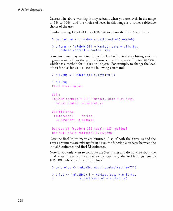
9. Robust Regression
Caveat: The above warning is only relevant when you use levels in the rangeof 1% to 10%, and the choice of level in this range is a rather subjectivechoice of the user.
Similarly, using level=0 forces lmRobmm to return the final M-estimates:
> control.mm <- lmRobMM.robust.control(level=0)
> oil.mm <- lmRobMM(Oil ~ Market, data = oilcity, + robust.control = control.mm)
Sometimes you may want to change the level of the test after fitting a robustregression model. For this purpose, you can use the generic function update,which has a method for "lmRobMM" objects. For example, to change the levelof test for bias for oil.s, use the following command:
> oil.tmp <- update(oil.s,level=0.2)
> oil.tmp
Final M-estimates.
Call:
lmRobMM(formula = Oil ~ Market, data = oilcity,
robust.control = control.s)
Coefficients:
(Intercept) Market
-0.08395777 0.8288791
Degrees of freedom: 129 total; 127 residual
Residual scale estimate: 0.1478398
Now the final M-estimates are returned. Also, if both the formula and thelevel arguments are missing for update, the function alternates between theinitial S-estimates and final M-estimates.
Note: If you only want to compute the S-estimates and do not care about thefinal M-estimates, you can do so by specifying the estim argument tolmRobMM.robust.control as follows:
> control.s <- lmRobMM.robust.control(estim="S")
> oil.s <- lmRobMM(Oil ~ Market, data = oilcity, + robust.control = control.s)
228

Controlling Options for Robust Regression
> oil.s
Initial S-estimates.
Call:
lmRobMM(formula = Oil ~ Market, data = oilcity, robust.control = control.s)
Coefficients:
(Intercept) Market
-0.06244374 0.8273216
Degrees of freedom: 129 total; 127 residual
Residual scale estimate: 0.1446283
Similarly, you can get the final M-estimates if you use estim=�MM�.
Resampling
Algorithms
When computing the initial S-estimates, a resampling scheme is used.S-PLUS provides three resampling algorithms for the initial S-estimates:random resampling, exhaustive resampling and genetic algorithm. Thesealgorithms can be selected by using the sampling argument to the functionlmRobMM.robust.control, for which the valid choices are "Random","Exhaustive" and "Genetic". Note that exhaustive resampling is onlyused/recommended when the sample size is small and there are less than 10predictor variables.
Random
Resampling
Parameters
Random resampling is controlled by two paramemters: a random seed andthe number of subsamples to draw. By default, the number of subsamples is
set at , where p is the number of explanatory variables, and [ ]denotes the operation of rounding a number to its closest integer. Note thatthis number will work fine if you have less than 13 predictor variables.However, if you have more than 13 predictor variables, the default numbermay be too big for computing in a reasonable time. To choose a differentvalue for the number of subsamples to draw, use the optional argument nrepas follows:
> oil.tmp <- lmRobMM(Oil~Market,data=oilcity,nrep=10)
The seed of the random resampling can be controlled by specifying theargument seed to lmRobMM.robust.control.
Genetic
Algorithm
Parameters
If you choose to use the genetic algorithm, the parameters for geneticalgorithm can be changed through the lmRobMM optional argumentgenetic.control, the default of which is NULL. The optional argument
4.6 2p⋅[ ]
229

9. Robust Regression
genetic.control should be a list, usually returned by a call to the functionlmRobMM.genetic.control. To look at the arguments of the functionlmRobMM.genetic.control, use the following command:
> args(lmRobMM.genetic.control)
function(popsize = NULL, mutate.prob = NULL, random.n = NULL, births.n = NULL, stock = list(), maxslen = NULL, stockprob = NULL, nkeep = 1)
For an explanation of the various arguments above, you should read the helpfile for the function ltsreg.default.
9.7 THEORETICAL DETAILS
Initial
Estimate
Details
The key to obtaining a good local minimum of the M-estimation objectivefunction when using a bounded, non-convex loss function is to compute a
highly robust initial estimate . S-PLUS does this by using the S-estimatemethod introduced by Rousseeuw and Yohai (1984), as part of an overallMM-estimate computational strategy proposed by Yohai, Stahel and Zamar(1991), and supported by a number of robustness experts who participated inthe 1989 IMA summer conference on �Directions in Robust Statistics andDiagnostics�.
The S-estimate approach has as its foundation an M-estimate of an
unknown scale parameter for observations , assumed to be
robustly centered (i.e., by subtracting a robust location estimate). The
M-estimate is obtained by solving the equation
where is a symmetric, bounded function. It is known that such a scale
estimate has a breakdown point of one-half (Huber, 1981), and that one canfind min-max bias robust M-estimates of scale (Martin and Zamar, 1989,1993).
(0.1)
β0
�sy y yn1 2, ,... ,
�s
15
1n
y
si
i
n
ρ�
=
=∑ .
ρ
230

Theoretical Details
The following regression S-estimate method was introduced by Rousseeuwand Yohai (1984). Consider the linear regression model modification of(3.7):
For each value of we have a corresponding robust scale estimate .
The regression S-estimate (which stands for �minimizing a robust scale
estimate�) is the value that minimizes :
This presents another non-linear optimization, one for which the solution istraditionally found by a random resampling algorithm, followed by a localsearch, as described in Yohai, Stahel and Zamar (1991). S-PLUS allows you touse a genetic algorithm in place of the resampling algorithm, and also to usean exhaustive form of sampling algorithm for small problems. Once the
initial S-estimate is computed, the final M-estimate is obtained as the
nearest local minimum of the M-estimate objective function.
For details on the numerical algorithms used, see Marazzi (1993), whosealgorithms, routines and code were used in creating lmRobMM.
Optimal and
Bisquare Rho
and Psi-
Functions
A robust M-estimate of regression coefficient is obtained by minimizing
where is a convex weight function of the residuals with tuning
constant c. The derivative of is usually denoted by . For
both the initial S-estimate and the final M-estimate in S-PLUS, two differentweight functions can be used: Tukey's bisquare function and an optimalweight function introduced in Yohai and Zamar (1998).
Tukey's bisquare functions and are as follows:,
(0.2)
(0.3)
15
1n p
y x
si i
T
i
n
−−
=
=∑ ρ
ββ�( )
.
β �( )s β
�β 0 �( )s β
� arg m in �( )β ββ0 = s
�β 0
β
ρβ
σ( ; ),y x
ci iT
i
n −
=∑
1
ρ( ; )⋅ cρ( ; )⋅ c ψ( ; )⋅ c
ρ( ; )⋅ c ψ( ; )⋅ c
ρ( ; )( ) ( ) ( )
r cr
c
r
c
r
cr c
r c
if
if = − + ≤
>
6 4 23 3
1
231

9. Robust Regression
The Yohai and Zamar optimal functions and are as follows:
where , , , , and
, , , .
The Efficient
Bias Robust
Estimate
Yohai and Zamar (1998) showed that the and functions given above areoptimal in the following highly desirable sense: the final M-estimate has abreakdown point of one-half, and minimizes the maximum bias undercontamination distributions (locally for small fractions of contamination),subject to achieving a desired efficiency when the data is Gaussian.
Efficiency
Control
The Gaussian efficiency of the final M-estimate is controlled by the choice ofthe tuning constant c. As discussed in the earlier sections, you can specify adesired Gaussian efficiency and S-PLUS will automatically use the correct cfor achieving that efficiency.
ψ ( ; )( ) ( ) ( )
r c c
r
c c
r
c c
r
cr c
r c
if
if = − + ≤
>
6 12 6
1
3 5
ρ( ; )⋅ c ψ( ; )⋅ c
ρ( ; )
.
[ . ( ) ( ) ( ) ( ) ]r
if
if
if
c
cr
c
c hr
ch
r
ch
r
ch
r
c
r
cr r
c
=
>
+ + + + < ≤
≤
325 3
1792 2 3
22
2
21
22
43
64
8
2
ψ( ; ) [ ( ) ( ) ( ) ]r
if
if
if
c
r
c
c gr
cg
r
cg
r
cg
r
c
r
c
rr
c
=
>
+ + + < ≤
≤
0 3
2 3
2
1 23
35
47
g1 1944= − . g2 1728= . g3 0312= − . g4 0 016= .
hg
11
2= h
g2
2
4= h
g3
3
6= h
g4
4
8=
ρ ψ
232

Theoretical Details
Robust
R-SquaredThe robust R2 is calculated as follows:
Initial S-Estimator
If an intercept term is included in the model, then
where and is the minimized , for a regression model with
only an intercept term with parameter . If there is no intercept term,
replace in the above formula with .
Final M-Estimator
If an intercept term is included in the model, then
where is the location M-estimate corresponding to the local minimum of
such that
where is the sample median estimate. If there is no intercept, replace with zero in the formula.
β0
R2 n 1–( )sy
2n p–( )se
2–
n 1–( )sy2
-------------------------------------------------=
se s0= sy s µ( )
µ
n 1–( )sy2
ns 0( )2
β1
µ
R2
ρyi µ–
s0
-------------
ρyi xi
Tβ–
s0
-------------------
∑–∑
ρyi µ–
s0
-------------
∑------------------------------------------------------------------------=
µ
Qy µ( ) ρyi µ–
s0
------------- ∑=
Qy µ( ) Qy µ*( )≤
µ* µ
233

9. Robust Regression
Robust
Deviance
For an M-estimate, the deviance is defined as the optimal value of the
objective function on the σ2-scale, that is:
Initial S-Estimator :
Final M-Estimator :
Robust F Test See chapter 7 of Hampel, Ronchetti, Rousseeuw and Stahel (1986), wherethis test is referred to as the �tau� test.
Robust Wald
Test
See chapter 7 of Hampel, Ronchetti, Rousseeuw and Stahel (1986).
Robust FPE
(RFPE)
Ronchetti (1985) proposed to generalize the Akaike Information Criterion(AIC) to robust model selection. However, the results therein are subject tocertain restrictions, such as they only apply to M-estimates with zerobreakdown point and the density of the errors has to be in a certain form.Yohai (1997) proposed the following RFPE criterion which is not subject tothe restrictions that apply to Ronchetti's robust version of AIC.
where
.
Since the first term in equation (12.4) can be approximated by
β0
D s2 β
0( ) s
0( )2
= =
β1
D 2 s0( )
2ρ
yi xiTβ
1–
s0
---------------------
∑⋅ ⋅=
(0.4)RFPE nEρ εσ---
pA
2B-------+=
A Eψ2 εσ---
= B Eψ′ εσ---
=
nEρ εσ---
ρr i
σ---
pA
2B-------+
i 1=
n
∑≈
234

Other Robust Regression Techniques
where , the expression (12.4) can be estimated by
with
The approximation on the right hand side of (12.5) is used as our RFPE.
9.8 OTHER ROBUST REGRESSION TECHNIQUES
Least Trimmed
Squares
Regression
Least trimmed squares regression (LTS) regression, introduced by Rousseeuw,1984, is a highly robust method for fitting a linear regression model. The
LTS estimate minimizes the sum of the q smallest squared residuals
where is the ith ordered residual. The value of q is often set to be
slightly larger than half of n.
By contrast, the ordinary least squares estimate minimizes the sum of all
of the squared residuals.
The least squares estimator lacks robustness because a single �observation� (yi,
xiT ) can cause to take on any value. The same is true of M-estimators of
regression, which are discussed in the section M-Estimates of Regression.
(0.5)
r i yi xiTβ
1–=
RFPE ρyi xi
Tβ1
–
s0( )
---------------------
i 1=
n
∑ pA
B---+≈
A1n--- ψ2
r i
s0( )
--------
i 1=
n
∑= B1n--- ψ′
r i
s0( )
--------
i 1=
n
∑=
(9.1)
(9.2)
bLTS
r i( )2
b( )i 1=
q
∑
r i( ) b( )
bLS
r i2b( )
i 1=
n
∑
bLS
235

9. Robust Regression
To compute the least trimmed squares regression, use the ltsreg function.For example, for the stack loss data, we can compute the LTS estimate asfollows:
> stack.df <- data.frame(stack.loss, stack.x)
> stack.lts <- ltsreg(stack.loss ~ ., stack.df)
> stack.lts
Method:
Least Trimmed Squares Robust Regression.
Call:
ltsreg.formula(stack.loss ~ ., stack.df)
Coefficients:
Intercept Air.Flow Water.Temp Acid.Conc.
-36.2921 0.7362 0.3691 0.0081
Scale estimate of residuals: 1.038
Total number of observations: 21
Number of observations that determine the LTS estimate: 13
Comparing the coefficients to those for the least-squares fit, we observe thatthe LTS values are noticeably different:
> stack.lm <- lm(stack.loss ~ ., stack.df)
> coef(stack.lm) (Intercept) Air.Flow Water.Temp Acid.Conc.
-39.91967 0.7156402 1.295286 -0.1521225
> coef(stack.lts)
Intercept Air Flow Water Temp Acid Conc.
-36.29212 0.7361645 0.3691111 0.008085206
A plot of the residuals versus the fitted values for the two fits is also revealing:
> par(mfrow=c(1,2))
> plot(fitted(stack.lm), resid(stack.lm),
+ ylim=range(resid(stack.lts)))
> plot(fitted(stack.lts), resid(stack.lts))
The resulting plot is shown in figure 9.5. The plot on the left shows theresiduals scattered with no apparent pattern; the plot on the right shows fourclear outliers�three at the top and one at the bottom.
236

Other Robust Regression Techniques
The LTS estimator has the highly attractive robustness property that itsbreakdown point is approximately 1/2 (if q is the right fraction of n). Thebreakdown point of a regression estimator is the largest fraction of data whichmay be replaced by arbitrarily large values without making the Euclidean
norm of the resulting estimate tend to ∞. The Euclidean norm is
defined as follows: .
To illustrate the concept of breakdown point, consider the simple problem ofestimating location, where often the estimator is the sample mean
. The breakdown point of the mean estimator is 0, since if
any single , then . On the other hand, the sample median
has breakdown point approximately 1/2, since, taking the case of an oddsample size n for convenience, one can move (n - 1)/2 of the observations yi
to ±∞ without taking the median to ±∞.
Any estimator with breakdown point approximately 1/2 is called a highbreakdown point estimator. Thus, the LTS estimator is a high breakdownpoint regression estimator.
The high breakdown point of the LTS estimator means that the values
, i = 1, ..., n , fit the bulk of the data well, even when the bulk of the
data may consist of only somewhat more than 50% of the data.
Figure 9.5: Residual plots for least-squares (left) and least trimmedsquares regression.
•
•
••
••••
•
•••
••
••
•••
•
•
fitted(stack.lm)
resi
d(st
ack.
lm)
10 20 30 40
-50
5
•
•
••
••••
••••••
•••••
•
•
fitted(stack.lts)
resi
d(st
ack.
lts)
10 15 20 25 30
-50
5
b
b2
b i2
i 1=
p∑=
y 1n--- yii 1=
n∑=
yi ∞±→ y ∞±→
xiTbLTS
237

9. Robust Regression
Correspondingly, the residuals will reveal the
outliers quite clearly. Least squares residuals and M-
estimate residuals often fail to reveal problems in the
data. This can be illustrated as follows.
First construct an artificial data set with 60 percent of the data scatteredabout the line yi = xi and the remaining 40 percent in an outlying cluster
centered at (6, 2).
> set.seed(14) #set the seed to reproduce this example
> x30 <- runif(30, .5, 4.5)
> e30 <- rnorm(30, 0, .2); y30 <- 2+x30+e30
> x20 <- rnorm(20, 6, .5); y20 <- rnorm(20, 2, .5)
> x <- c(x30, x20)
> y <- c(y30, y20)
Plot the data, then fit and label 3 different regression lines: the ordinary leastsquares line, an M-estimate line, and the least trimmed squared residuals line.
> plot(x, y)
> abline(lm(y ~ x))
> text(5, 3.4, "LS")
> abline(rreg(x, y))
> text(4, 3.2, "M")
> abline(ltsreg(x, y))
> text(4, 6.5, "LTS")
The resulting plot is shown in figure 9.6.
The outlying points pull both the ordinary least squares line and the M-estimate away from the bulk of the data. Neither of these two fitting methodsis robust to outliers in the x direction. (Such outliers are called leverage pointsin the literature.) The LTS line recovers the linear structure in the bulk of thedata and essentially ignores the outlying cluster. In higher dimensions suchoutlying clusters are very hard to identify using classical regressiontechniques.
r i bLTS( ) yi xiTbLTS–=
r i bLS( ) yi xiTbLS–=
r i bM( ) yi xiTbM–=
238

Other Robust Regression Techniques
Least Median
Squares
Regression
An idea quite similar to LTS regression is least median squares or LMSregression. Rather than minimizing the sum of the squared residuals as leastsquares regression does, least median of squares (Rousseeuw, 1984)minimizes the median of the squared residuals. The lmsreg functionperforms LMS regression.
Least median of squares regression has a very high breakdown point of almost50%. That is, almost half of the data can be corrupted in an arbitrary fashionand the least median of squares estimates continue to follow the majority ofthe data. At the present time this property is virtually unique among therobust regression methods that are publicly available.
However, least median of squares is statistically very inefficient. It is due tothis inefficiency that we recommend lmRobMM and ltsreg over lmsreg.
Least Absolute
Deviation
Regression
The idea of least absolute deviation regression, or L1 regression, is actuallyolder than that of least-squares, but until the development of high-speedcomputers, it was too cumbersome to have wide applicability. S-PLUS has thefunction l1fit (note that the second character in the function name is thenumber �1�, not the letter �l�) for computing least absolute deviationregression. As its name implies, least absolute deviation regression finds the
estimate that minimizes the sum of the absolute values of the residuals
Figure 9.6: Least trimmed squares regression, compared to least-squaresand M-estimates.
••
•
•
•
•
•
•
•
•
•
•
•
••
•
•
••
•
•
•
•
•
•
•
•
•
•
•
•
•••
•••
••
•
•
•
•
•
•
•
•
•
••
x
y
1 2 3 4 5 6 7
12
34
56
LSM
LTS
bL1
239

9. Robust Regression
.
As an example, consider again the stack loss data. We construct the L1regression using l1fit as follows:
> stack.l1 <- l1fit(stack.x, stack.loss)
> stack.l1
$coefficients:
Intercept Air Flow Water Temp Acid Conc.
-39.68984 0.8318844 0.5739114 -0.06086962
$residuals:
[1] 5.06086922 0.00000000 5.42898512 7.63478470
[5] -1.21739304 -1.79130435 -1.00000000 0.00000000
[9] -1.46376634 -0.02029470 0.52752948 0.04057107
[13] -2.89855528 -1.80290544 1.18260598 0.00000000
[17] -0.42608732 0.00000000 0.48695821 1.61739087
[21] -9.48116493
Plotting the residuals against fitted values and comparing the plot to thecorresponding plot for the least-squares fit shows the outliers clearly, thoughnot so clearly as for the ltsreg plot.
> plot(fitted(stack.lm), resid(stack.lm))
> plot(stack.loss - resid(stack.l1), resid(stack.l1))
The plot is shown in figure 9.7.
Figure 9.7: Residual plots for least-squares (left) and least absolutedeviation regression.
r i b( )i 1=
n
∑
•
•
••
••••
•
•••
••
••
•••
•
•
fitted(stack.lm)
resi
d(st
ack.
lm)
10 20 30 40
-6-2
24
6
•
•
••
••••
••••
••
•• •••
•
•
stack.loss - resid(stack.l1)
resi
d(st
ack.
l1)
10 20 30
-10
-50
5
240

Other Robust Regression Techniques
M-Estimates of
Regression
The M-estimator of regression was introduced by Huber in 1973. An M-
estimate of regression is the b which minimizes
for a given ρ. Least squares corresponds to ρ(x) = x2 and least absolutedeviation regression corresponds to ρ(x) = |x|. Generally, although not in the
two cases mentioned above, the value of is dependent on the value of σ,
which is usually unknown.
Although M-estimates are protected against wild values in the response y,they are susceptible to high leverage points�that is, points which have quitedifferent x-values relative to the other observations. In particular, atypographical error in an explanatory variable can have a dramatic affect onan M-estimate, while least trimmed squares regression handles this situationeasily. One advantage of M-estimates is that they can be computed in muchless time than least trimmed squares or other high-breakdown estimates.
M-estimates in S-PLUS are calculated using the rreg function to perform aniteratively reweighted least-squares fit. What this means is that S-PLUS
calculates an initial fit (using traditional weighted least-squares, by default),then calculates a new set of weights based on the results of the initial fit. Thenew weights are then used in another weighted least-squares fit, new weightsare calculated, and so on, iteratively, until either some convergence criteriaare satisfied or a specified maximum number of iterations is reached.
The only required arguments to rreg are x, the vector or matrix ofexplanatory variables, and y, the vector response:
> stack.M1 <- rreg(stack.x, stack.loss)
> stack.M1
$coefficients:
(Intercept) Air Flow Water Temp Acid Conc.
-42.07438 0.8978265 0.731816 -0.1142602
$residuals:
[1] 2.65838630 -2.45587390 3.72541082 6.78619020
[5] -1.75017776 -2.48199378 -1.52824862 -0.52824862
[9] -1.89068795 -0.03142924 0.99691253 0.61446835
[13] -2.80290885 -1.27786270 2.17952419 0.83674360
[17] -0.49471517 0.30510621 0.68755039 1.52911203
[21] -10.01211661
(9.1)
bM
ρr i b( )
σ------------
i 1=
n
∑
bM
241

9. Robust Regression
$w:
[1] 0.87721539 0.91831885 0.77235329 0.41742415 0.95387576
[6] 0.90178786 0.95897484 0.99398847 0.93525890 0.99958817
[11] 0.97640677 0.98691782 0.89529949 0.98052477 0.92540436
[16] 0.98897286 0.99387986 0.99933718 0.99574820 0.96320721
[21] 0.07204303
You control the choice of ρ in rreg by specifying a weight function as themethod argument. There are eight weight functions built into S-PLUS; thereis not yet a consensus on which is �best.� See the rreg help file for details onthe weight functions. The default weight function uses Huber�s weightfunction until convergence, then a bisquare weight function for two moreiterations. The following call to rreg defines a simple weight function thatcorresponds to the least-squares choice ρ = x2:
> stack.MLS <- rreg(stack.x,stack.loss,
+ method=function(u) 2*abs(u),iter=100)
Warning messages:
failed to converge in 100 steps in:
rreg(stack.x, stack.loss, method = function(u) ....
> stack.MLS$coef
(Intercept) Air Flow Water Temp Acid Conc.
-39.70404 0.7165807 1.298218 -0.1561163
> coef(stack.lm)
(Intercept) Air.Flow Water.Temp Acid.Conc.
-39.91967 0.7156402 1.295286 -0.1521225
9.9 APPENDIX
The function gen.data used in the section Robust Model Selection is asfollows:
> gen.data <- function(coeff, n = 100, eps = 0.1, sig = 3,
+ snr = 1/20, seed = 837)
+ {
+ # coeff : 3 x 1 vector of coefficients
+ # eps : the contamination ratio, between 0 and 0.5
+ # sig : standard deviation of most observations
+ # snr : signal-to-noise ratio, well, not really
+ # Note : the regressors are generated as: rnorm(n,1),
+ # rnorm(n,1)^3, exp(rnorm(n,1)). It also generates
+ # an unused vector x4.
+ set.seed(seed)
242

Bibliography
+ x <- cbind(rnorm(n, 1), rnorm(n, 1)^3, + exp(rnorm(n, 1)))
+ ru <- runif(n)
+ n1 <- sum(ru < eps)
+ u <- numeric(n)
+ u[ru < eps] <- rnorm(n1, sd = sig/snr)
+ u[ru > eps] <- rnorm(n - n1, sd = sig)
+ data.frame(y = x %*% matrix(coeff, ncol = 1) + u,
+ x1 = x[,1], x2 = x[,2], x3 = x[,3],
+ x4 = rnorm(n, 1))
+ }
9.10 BIBLIOGRAPHY
Hampel, F., Ronchetti, E. M., Rousseeuw, P. J. and Stahel, W. A. (1986):Robust Statistics: the Approach Based on Influence Functions, John Wiley &Sons.
Huber, P.J. (1981). Robust Statistics. John Wiley & Sons.
Marazzi, A. (1993): Algorithms, Routines, and S Functions for Robust Statistics,Wadsworth & Brooks/Cole, Pacific Grove, CA.
Martin, R. D. and Zamar, R. H. (1989). Asymptotically Min-Max RobustM-estimates of Scale for Positive Random Variables. J. Amer. Statist. Assoc.,84, 494-501.
Martin, R. D. and Zamar, R. H. (1993). Bias Robust Estimates of Scale.Annals of Statistics.
Ronchetti, E. (1985): Robust Model Selection in Regression, S-PLUS
Statistics & Probability Letters, 3, 21--23.
Rousseeuw, P. J. (1984). Least median of squares regression. Journal of theAmerican Statistical Association, 79, 871-881.
Rousseeuw, P. J. and Yohai, V. (1984): Robust Regression by Means of S-estimators. In Robust and Nonlinear Time Series Analysis, J. Franke, W.Hardle, and R. D. Martin (eds.), Lecture Notes in Statistics, 26, 256-272,Springer-Verlag.
Yohai, V. J. (1987): High Breakdown-Point and High Efficiency Estimatesfor Regression, Annals of Statistics, 15, 642-665.
Yohai, V. J. (1997): A New Robust Model Selection Criterion for LinearModels: RFPE, unpublished note.
243

9. Robust Regression
Yohai, V., Stahel, W. A. and Zamar, R. H. (1991): A Procedure for RobustEstimation and Inference in Linear Regression, in Stahel, W. A. andWeisberg, S. W., Eds., Directions in Robust Statistics and Diagnostics, Part II,Springer-Verlag, New York.
Yohai, V. J. and Zamar (1998). �Optimal locally robust M-estimates ofregression�, Jour. of Statist. Inf. and Planning.
244

GENERALIZING THE LINEAR
MODEL 1010.1 Logistic Regression 247
Fitting a Linear Model 248
Fitting an Additive Model 253
Returning to the Linear Model 257
10.2 Poisson Regression 259
10.3 Generalized Linear Models 266
10.4 Generalized Additive Models 269
10.5 Quasi-Likelihood Estimation 270
10.6 Residuals 272
10.7 Prediction From the Model 274
Predicting the Additive Model of Kyphosis 274
Safe Prediction 276
10.8 References 277
245

10. Generalizing the Linear Model
246

GENERALIZING THE LINEAR MODEL 10The use of least squares estimation of regression coefficients for linear modelsdates back to the early nineteenth century. It met with immediate success as asimple way of mathematically summarizing relationships between observedvariables of real phenomena. It quickly became and remains one of the mostwidely used statistical methods of practicing statisticians and scientificresearchers.
Because of the simplicity, elegance, and widespread use of the linear model,researchers and practicing statisticians have tried to adapt its methodology todifferent data configurations. For example, there is no reason conceptuallywhy a categorical response or some transformation of it could not be relatedto a set of predictor variables in a similar way to the continuous response ofthe linear model. Although conceptually plausible, developing regressionmodels for categorical responses lacked solid theoretical foundation until theintroduction of the generalized linear model by Nelder and Wedderburn(1972).
This chapter focuses on generalized linear models and their generalization,generalized additive models, as they apply to categorical responses. Inparticular, we focus on logistic and Poisson regressions and also include abrief discussion of the fitting of models when you can�t specify an exactlikelihood, using the quasi-likelihood method.
10.1 LOGISTIC REGRESSIONTo fit a logistic regression model, use either the glm function or the gamfunction with a formula to specify the model and the family argument setto binomial. In this case the response variable is necessarily binary or two-valued. As an example, consider the built-in data frame kyphosis. Asummary of the data frame produces the following:
> attach(kyphosis)
> summary(kyphosis)
Kyphosis Age Number Start
absent :64 Min. : 1.00 Min. : 2.000 Min. : 1.00
present:17 1st Qu.: 26.00 1st Qu.: 3.000 1st Qu.: 9.00
Median : 87.00 Median : 4.000 Median :13.00
Mean : 83.65 Mean : 4.049 Mean :11.49
3rd Qu.:130.00 3rd Qu.: 5.000 3rd Qu.:16.00
Max. :206.00 Max. :10.000 Max. :18.00
247

10. Generalizing the Linear Model
The four variables in kyphosis are defined as follows:
Kyphosis A binary variable indicating the presence/absence of apostoperative spinal deformity called Kyphosis.
Age The age of the child in months.
Number The number of vertebrae involved in the spinal operation.
Start The beginning of the range of the vertebrae involved in theoperation.
A convenient way of examining the bivariate relationship between eachpredictor and the binary response, Kyphosis, is with a set of boxplotsproduced by plot.factor:
> par(mfrow=c(1,3), cex = .7)
> plot.factor(kyphosis)
Setting the mfrow parameter to c(1,3) produces three plots in a row. The
character expansion is set to 0.7 times the normal size using the cexparameter of the par function. Figure 10.1 displays the result.
Both Start and Number show strong location shifts with respect to thepresence or absence of Kyphosis. Age does not show such a shift inlocation.
Fitting a
Linear Model
The logistic model we start with relates the probability of developingKyphosis to the three predictor variables, Age, Number and Start. We fitthe model using glm as follows:
> kyph.glm.all <- glm(Kyphosis ~ Age + Number + Start,
+ family = binomial, data = kyphosis)
Figure 10.1: Boxplots of the predictors of kyphosis versus Kyphosis.
050
100
150
200
Age
absent present
Kyphosis
24
68
10
Num
ber
absent present
Kyphosis
510
15
Sta
rt
absent present
Kyphosis
248

Logistic Regression
The summary function produces a summary of the resulting fit:
> summary(kyph.glm.all)
Call: glm(formula = Kyphosis ~ Age + Number + Start,
family = binomial, data = kyphosis)
Deviance Residuals:
Min 1Q Median 3Q Max
-2.312363 -0.5484308 -0.3631876 -0.1658653 2.16133
Coefficients:
Value Std. Error t value
(Intercept) -2.03693225 1.44918287 -1.405573
Age 0.01093048 0.00644419 1.696175
Number 0.41060098 0.22478659 1.826626
Start -0.20651000 0.06768504 -3.051043
(Dispersion Parameter for Binomial family taken to be 1 )
Null Deviance: 83.23447 on 80 degrees of freedom
Residual Deviance: 61.37993 on 77 degrees of freedom
Number of Fisher Scoring Iterations: 5
Correlation of Coefficients:
(Intercept) Age Number
Age -0.4633715
Number -0.8480574 0.2321004
Start -0.3784028 -0.2849547 0.1107516
The summary includes:
1. a replica of the call that generated the fit,
2. a summary of the deviance residuals (more on these later),
3. a table of estimated regression coefficients, their standard errors, andthe partial t-test of their significance,
4. estimates of the null and residual deviances (more on these later),and
5. a correlation matrix of the coefficient estimates.
The partial t-tests indicate that Start is important even after adjusting forAge and Number, but they provide little information on the other twovariables.
249

10. Generalizing the Linear Model
You can produce an analysis of deviance for the sequential addition of eachvariable by using the anova function, specifying the chi-square test to test fordifferences between models:
> anova(kyph.glm.all, test = "Chi")
Analysis of Deviance Table
Binomial model
Response: Kyphosis
Terms added sequentially (first to last)
Df Deviance Resid. Df Resid. Dev Pr(Chi)
NULL 80 83.23447
Age 1 1.30198 79 81.93249 0.2538510
Number 1 10.30593 78 71.62656 0.0013260
Start 1 10.24663 77 61.37993 0.0013693
Here we see that Number is important after adjusting for Age. We alreadyknow that Number loses its importance after adjusting for Age and Start.Age does not appear to be important as a linear predictor.
You can examine the bivariate relationships between the probability ofKyphosis and each of the predictors by fitting a �null� mode and then addingeach of the terms, one at a time:
> kyph.glm.null <- glm(Kyphosis ~ 1, family = binomial,
+ data = kyphosis)
> add1(kyph.glm.null, ~ . + Age + Number + Start)
Single term additions
Model: Kyphosis ~ 1
Df Sum of Sq RSS Cp
<none> 81.00000 83.02500
Age 1 1.29546 79.70454 83.75454
Number 1 10.55222 70.44778 74.49778
Start 1 16.10805 64.89195 68.94195
The Cp statistic is used to compare models that are not nested. A small Cpcorresponds to a better model in the sense of smaller residual deviancepenalized by the number of parameters that are estimated in fitting themodel.
Clearly Start is the best single variable to use in a linear model. Thesestatistical conclusions, however, should be verified by looking at graphicaldisplays of the fitted values and residuals.
250

Logistic Regression
The plot method for generalized linear models produces four plots:
1. a plot of deviance residuals versus the fitted values.
2. a plot of the square root of the absolute deviance residuals versus thelinear predictor values.
3. a plot of the response versus the fitted values.
4. a Normal quantile plot of the Pearson residuals.
This set of plots is similar to those produced by the plot method for lmobjects.
Systematic curvature in the residual plots could be indicative of problems inthe choice of link, wrong scale of one of the predictors, or omission of aquadratic term in a predictor. Large residuals can be also be detected withthese plots. These may be indicative of the need to remove the correspondingobservations and re-fit the model. The plot of the absolute residuals againstpredicted values gives a visual check on the adequacy of the assumed variancefunction.
The Normal quantile plot is also generated for glm objects. This plot couldbe useful in the detection of extreme observations deviating from a generaltrend but one should exercise caution in not over-interpreting its shape,which is not necessarily of interest in the nonlinear context.
Figure 10.2 results from simply plotting the fit. Residual plots are not usefulfor binary data, such as Kyphosis, because all of the points line on one oftwo curves depending on whether the response is 0 or 1.
> par(mfrow=c(2,2))
> plot(kyph.glm.all, ask=F)
A more useful diagnostic plot is produced by plot.gam. By default,plot.gam plots the estimated relationship between the individual fittedterms and each of the corresponding predictors. You can request that partialresiduals be added to the plot by specifying the argument resid=T. The scaleargument can be used to keep all of the plots on the same scale to easecomparison. Figure 10.3 is produced by plot.gam:
> par(mfrow=c(1,3))
> plot.gam(kyph.glm.all, resid = T, scale = 6)
These plots give a quick assessment of how well the model fits the datathrough examination of the fit of each term in the formula. The plots are ofthe adjusted relationship for each predictor versus each predictor. When therelationship is specified as linear the label on the vertical axis reduces to thevariable name. We will see the utility of this plot method and the reason forthe labels when we plot additive models produced by gam.
251

10. Generalizing the Linear Model
Figure 10.2: Plots of the generalized linear model of Kyphosispredicted by Age, Start, and Number.
Figure 10.3: Additional plots of the generalized linear model ofKyphosis predicted by Age, Number, and Start.
••
•
•
•••••
••
•
•
••••
•• •
•
•
•
•
•
• ••• •• • ••
•••
•
•
•
•
•
•
•
•
•
• •
•
• ••
••
•••
•
••
••
•
•••• •••
•••
•
••
•
••
•
•
Fitted : Age + Number + StartD
evia
nce
Res
idua
ls0.0 0.2 0.4 0.6 0.8
-2-1
01
2
••
••
•• • • •
••
•
•
••
•
•
•
••
•
•
•
• •
••
•
••
•
••
•
•
• •
•
•
•
•
•
•
•
•
•
••
•
••
•
•
•
•••
••
•
•••
• •••
•
••
••
•
•
•
•
•
••
•
•
Predicted : Age + Number + Start
sqrt
(abs
(res
id(k
yph.
glm
.all)
))
-4 -2 0 2
0.4
0.8
1.2
••
•
••••••
••
• •••• • •• ••
••
•
•
• ••• •• • •• •••
•
•
• •
• •••
•
• •
•
• ••
•
• •••
•
••
••
••••• ••• ••• •• •
•
••
•
•
Fitted : Age + Number + Start
Kyp
hosi
s
0.0 0.4 0.8
0.0
0.4
0.8
• •
•
•• ••••
••
••
•• ••• •• ••
•
•
•
•• • •• ••• ••
••
•
•
•
••
•
••
•
••
•
•••••• • •
•
••
• •
•••• •• • •• • •
•••
•
• •
•
•
Quantiles of Standard NormalP
ears
on R
esid
uals
-2 -1 0 1 2
-20
2
Age
Age
0 100 200
-20
12
3
•
•
•
•••
•••
••
•
••
•
••
••
••
•
•
••
••
••
•
•••• ••
•
•
•
•
•
•••
•
•
••
•
•
••
•
•
••
•
•
•
•
••
•
••
•
••
••
••••
•
•
•
•
••
•
Number
Num
ber
2 4 6 8 10
-20
12
3
••
•
••
•••
•
••
• ••
••
•••
••
••
•
•
•
•••••
•
•• •••
•
•
•
•
••
••
•
• •
•
•
••
•
••
••
•
•
•
•
•
•• ••
•••
••••
•• •
•
•
•
•
•
Start
Sta
rt
0 5 10
-20
12
3
•
•
•
•
•••••
• •
•
•
•
•••• •
•
•
• •
•
•
•
•
• ••••
• ••
•
•
•
•
•
•
••
•
•
•
••
•
••
•
•
••••
•
• •
•
•
•
••
•
••
•
•••
•• •
•
•
••
•
•
252

Logistic Regression
Both plot.glm (the underlying plotting method for generalized linearmodels) and plot.gam produce multiple plots; you can, however, choosewhich plots you look at by using the argument ask=T (the default). Thisproduces a menu of available plots; you then select the number of the desiredplot. For example, here is the menu of default GLM plots for the functionkyph.glm.all:
> plot(kyph.glm.all, ask=T)
Make a plot selection (or 0 to exit):
1: plot: All
2: plot: Residuals vs Fitted Values
3: plot: Sqrt of abs(Residuals) vs Predictions
4: plot: Response vs Fitted Values
5: plot: Normal QQplot of Std. Residuals
Selection:
Fitting an
Additive Model
So far we have examined only linear relationships between the predictors andthe probability of developing Kyphosis. We can assess the validity of thelinear assumption by fitting an additive model with relationships estimatedby smoothing operations (cubic splines or local regression) and comparing itto the linear fit. We use the gam function to fit additive models.
> kyph.gam.all <-
+ gam(Kyphosis ~ s(Age) + s(Number) + s(Start),
+ family = binomial, data = kyphosis)
Including each variable as an argument to the s function instructs gam toestimate the �smoothed� relationships with each predictor by using cubic B-splines. Alternatively we could have used the lo function for local regressionsmoothing (loess). A summary of the fit is:
> summary(kyph.gam.all)
Call: gam(formula = Kyphosis ~ s(Age) +s(Number)+ s(Start),
family = binomial, data = kyphosis)
Deviance Residuals:
Min 1Q Median 3Q Max
-1.351358 -0.4439636 -0.1666238 -0.01061843 2.10851
(Dispersion Parameter for Binomial family taken to be 1 )
Null Deviance: 83.23447 on 80 degrees of freedom
253

10. Generalizing the Linear Model
Residual Deviance: 40.75732 on 68.1913 degrees of freedom
Number of Local Scoring Iterations: 7
DF for Terms and Chi-squares for Nonparametric Effects
Df Npar Df Npar Chisq P(Chi)
(Intercept) 1
s(Age) 1 2.9 5.782245 0.1161106
s(Number) 1 3.0 5.649706 0.1289318
s(Start) 1 2.9 5.802950 0.1139286
The summary of a gam fit is similar to the summary of a glm fit. Onenoticeable difference is the analysis of deviance table. For the additive fit thetests correspond to approximate partial tests for the importance of the smoothfor each term in the model. These tests are typically used for screeningvariables for inclusion in the model. The approximate nature of these tests isdiscussed in detail in Hastie and Tibshirani (1990). For a single variable inthe model, this is equivalent to testing for a difference between a linear fitand a smooth fit which includes a linear term along with the smooth term.
Now let�s fit two additional models, adding a smooth of each of Age andNumber to the base model which has a smooth of Start.
> kyph.gam.start.age <-
+ gam(Kyphosis ~ s(Start) + s(Age),
+ family = binomial, data = kyphosis)
> kyph.gam.start.number <-
+ gam(Kyphosis ~ s(Start) + s(Number),
+ family = binomial, data = kyphosis)
We produce the following analysis of deviance tables:
> anova(kyph.gam.start, kyph.gam.start.age, test="Chi")
Analysis of Deviance Table
Response: Kyphosis
Terms Resid. Df Resid. Dev
1 s(Start) 76.24543 59.11262
2 s(Start) + s(Age) 72.09458 48.41713
Test Df Deviance Pr(Chi)
1
2 +s(Age) 4.150842 10.69548 0.0336071
254

Logistic Regression
> anova(kyph.gam.start, kyph.gam.start.number,
+ test="Chi")
Analysis of Deviance Table
Response: Kyphosis
Terms Res.Df Res.Dev
1 s(Start) 76.245 59.1126
2 s(Start)+s(Number) 72.180 54.1790
Test Df Deviance Pr(Chi)
1
2 +s(Number) 4.064954 4.933668 0.3023856
The indication is that Age is important in the model even with Startincluded whereas Number isn�t important under the same conditions.
You can plot the fit with a smooth on Age and Start adding partial residualswhile maintaining all figures on the same scale as follows:
> par(mfrow = c(2,2))
> plot(kyph.gam.start.age, resid = T, scale = 8)
Or you can simply plot the fit adding pointwise confidence intervals for thefit.
> plot(kyph.gam.start.age, se = T, scale = 10)
Figure 10.4 displays the resulting plots produced by plot.gam. Notice thevertical axes labels now. They reflect the smoothing operation included in themodeling.
The summary of the additive fit with smooths of Age and Start includedappears as follows:
> summary(kyph.gam.start.age)
Call: gam(formula = Kyphosis ~ s(Start) + s(Age),
family = binomial, data = kyphosis)
Deviance Residuals:
Min 1Q Median 3Q Max
-1.694389 -0.4212112 -0.1930565 -0.02753535 2.087434
(Dispersion Parameter for Binomial family taken to be 1 )
Null Deviance: 83.23447 on 80 degrees of freedom
Residual Deviance: 48.41713 on 72.09458 degrees of freedom
255

10. Generalizing the Linear Model
Number of Local Scoring Iterations: 6
DF for Terms and Chi-squares for Nonparametric Effects
Df Npar Df Npar Chisq P(Chi)
(Intercept) 1
s(Start) 1 2.9 7.729677 0.0497712
s(Age) 1 3.0 6.100143 0.1039656
Figure 10.4: The partial fits for the generalized additive logistic regressionmodel of Kyphosis with Age and Start as predictors.
Start
s(S
tart
)
5 10 15
-6-4
-20
2
•
•
•
•
•
•
•
••
•
•
•
••
•
•
•
•
•
•
•
•
•
•
•
•
•
•
•••
••
•
•
•
•
•
••
•
•••
•
•
•
•
•
•
•
•
•
•
••
•
•
•
•
• •
•
•
•
•
•
•
•
••
•
•
••
•
••
•
•
Age
s(A
ge)
0 50 100 150 200
-4-2
02
4
••
•
•••
•
•
•
•
•
•
••
•
•
•
•
•
••
••
•
•
••
•
•
•
•••
•
•
•
•
•
•
••
• ••
••
••
•
••
•
•
•
••
•
•
•
•
••
•
•
••
•
••
••
•
••
•
•
•
••
•
Start
s(S
tart
)
5 10 15
-10
-50
Age
s(A
ge)
0 50 100 150 200
-6-4
-20
2
256

Logistic Regression
Returning to
the Linear
Model
The plots of the fits of the additive model displayed in figure 10.4 suggest aquadratic relationship for Age and a piecewise linear relationship for Start.It is useful to fit these suggested relationships as a linear model if the model isfurther simplified without losing too much precision in predicting theresponse.
For Age we fit a second degree polynomial. For Start, recall that its valuesindicate the beginning of the range of the vertebrae involved in theoperation. Values less than or equal to 12 correspond to the thoracic regionof the spine and values greater than 12 correspond to the lumbar region.Since the relationship for Start is fairly flat for values of Startapproximately less than or equal to 12, and then drops off linearly for valuesgreater than 12, we will try fitting a linear model with the term I((Start -12) * (Start > 12)). The I function is used here to prevent the "*"from being used for factor expansion in the formula sense.
Figure 10.5 displays the resulting fit along with the partial residuals as well asthe fit along with two standard errors bands.
The summary of the fit follows:
> summary(kyph.glm.istart.age2)
Call: glm(formula = Kyphosis ~ poly(Age, 2) +
I((Start - 12) * (Start > 12)), family = binomial,
data = kyphosis)
Deviance Residuals:
Min 1Q Median 3Q Max
-1.42301 -0.5014355 -0.1328078 -0.01416602 2.116452
Coefficients:
Value Std. Error t value
(Intercept) -0.6849607 0.4570976 -1.498500
poly(Age, 2)1 5.7719269 4.1315471 1.397038
poly(Age, 2)2 -10.3247767 4.9540479 -2.084109
I((Start-12)*(Start>12)) -1.3510122 0.5072018 -2.663658
(Dispersion Parameter for Binomial family taken to be 1 )
Null Deviance: 83.23447 on 80 degrees of freedom
Residual Deviance: 51.95327 on 77 degrees of freedom
Number of Fisher Scoring Iterations: 6
257

10. Generalizing the Linear Model
Correlation of Coefficients:
(Intercept) poly(Age,2)1 poly(Age,2)2
poly(Age, 2)1 -0.1133772
poly(Age, 2)2 0.5625194 0.0130579
I((Start-12)*(Start>12)) -0.3261937 -0.1507199 -0.0325155
Figure 10.5: The partial fits for the generalized linear logistic regressionmodel of Kyphosis with quadratic fit for Age and piecewise linear fitfor Start.
Age
poly
(Age
, 2)
0 50 100 150 200
-4-2
02
4
• •
•
•••
••
••
•
•
••
•
•
•
•
•
••
••
•
•
••
•
•
•• •
•
•
•
•
•
•
•
••
• ••
••
••
•
••
•
•
•
••
•
•
•
•
••
•
•
• •
•
••
••
•
•
••
•
•
•
•
•
Start
I((S
tart
- 1
2) *
(S
tart
> 1
2))
0 5 10 15
-6-4
-20
24
•
•
•
•
•
•
•
••
•
•
•
• •
•
•
•
•
•
•
•
• •
•
•
•
•
•
•••
••
•
•
•
•
•
•
••
•••
•
•
•
•
•
•
•
•
•
•
••
•
•
•
•
• •
•
•
•
•
•
•
•
•
•
•
•
••
•
••
•
•
Age
poly
(Age
, 2)
0 50 100 150 200
-8-6
-4-2
02
4
Start
I((S
tart
- 1
2) *
(S
tart
> 1
2))
5 10 15
-8-6
-4-2
02
4
258
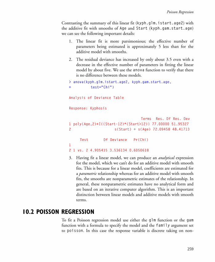
Poisson Regression
Contrasting the summary of this linear fit (kyph.glm.istart.age2) withthe additive fit with smooths of Age and Start (kyph.gam.start.age)we can see the following important details:
1. The linear fit is more parsimonious; the effective number ofparameters being estimated is approximately 5 less than for theadditive model with smooths.
2. The residual deviance has increased by only about 3.5 even with adecrease in the effective number of parameters in fitting the linearmodel by about five. We use the anova function to verify that thereis no difference between these models.
> anova(kyph.glm.istart.age2, kyph.gam.start.age,
+ test="Chi")
Analysis of Deviance Table
Response: Kyphosis
Terms Res. Df Res. Dev
1 poly(Age,2)+I((Start-12)*(Start>12)) 77.00000 51.95327
2 s(Start) + s(Age) 72.09458 48.41713
Test Df Deviance Pr(Chi)
1
2 1 vs. 2 4.905415 3.536134 0.6050618
3. Having fit a linear model, we can produce an analytical expressionfor the model, which we can�t do for an additive model with smoothfits. This is because for a linear model, coefficients are estimated fora parametric relationship whereas for an additive model with smoothfits, the smooths are nonparametric estimates of the relationship. Ingeneral, these nonparametric estimates have no analytical form andare based on an iterative computer algorithm. This is an importantdistinction between linear models and additive models with smoothterms.
10.2 POISSON REGRESSION
To fit a Poisson regression model use either the glm function or the gamfunction with a formula to specify the model and the family argument setto poisson. In this case the response variable is discrete taking on non-
259

10. Generalizing the Linear Model
negative integer values. Count data is frequently modeled as a Poissondistribution. As an example, consider the built-in data framesolder.balance. A summary of the data frame produces the following:
> attach(solder.balance)
> summary(solder.balance)
Opening Solder Mask PadType Panel skips
S:240 Thin :360 A1.5:180 L9 : 72 1:240 Min. : 0.000
M:240 Thick:360 A3 :180 W9 : 72 2:240 1st Qu.: 0.000
L:240 B3 :180 L8 : 72 3:240 Median : 2.000
B6 :180 L7 : 72 Mean : 4.965
D7 : 72 3rd Qu.: 6.000
L6 : 72 Max. :48.000
(Other):288
The solder experiment, contained in solder.balance, was designed andimplemented in one of AT&T�s factories to investigate alternatives in the�wave-soldering� procedure for mounting electronic components on circuitboards. Five different factors were considered as having an effect on thenumber of solder skips. A brief description of each of the factors follows. Formore details, see the paper by Comizzoli, Landwehr, and Sinclair (1990).
Opening amount of clearance around the mounting pad
Solder amount of solder
Mask type and thickness of the material used for the solder mask
PadType the geometry and size of the mounting pad
Panel each board was divided into three panels, with three runs on aboard
skips number of visible solder skips on a circuit board.
Two useful preliminary plots of the data are a histogram of skips, theresponse, and plots of the mean response for each level of the predictor.Figure 10.6 and figure 10.7 display the resulting plots.
> par(mfrow=c(1,1))
> hist(skips)
> plot(solder.balance)
The histogram of skips in figure 10.6 shows the skewness and long-tailedness typical of count data. We will model this using a Poissondistribution.
260

Poisson Regression
Figure 10.6: A histogram of skips for solder data.
Figure 10.7: A plot of the mean response for each level of each factor.
0 10 20 30 40 500
100
200
skips
Factors
mea
n of
ski
ps
24
68
10
S
ML
Thin
Thick
A1.5
A3
B3
B6
W4D4
L4
D6
L6
D7
L7
L8
W9
L91
23
Opening Solder Mask PadType Panel
261

10. Generalizing the Linear Model
The plot of the mean skips for different levels of the factors displayed infigure 10.7 shows a very strong effect due to Opening. For levels M and Lonly about two skips were seen on average, whereas for level S, more then 10skips were seen. Effects almost as strong were seen for different levels ofMask.
If we do boxplots of skips for each level of the two factors, Opening andMask, we get an idea of the distribution of the data across levels of thefactors. Figure 10.8 displays the results of doing �factor� plots on these twofactors.
> par(mfrow=c(1,2))
> plot.factor(skips ~ Opening + Mask)
On examining figure 10.8, it is clear that the variance of skips increases asits mean increases. This is typical of Poisson distributed data.
We proceed now to model skips, using glm, as a function of the controlledfactors in the experiment declaring family = poisson. We start with asimple-effects model for skips as follows:
> paov <- glm(skips ~ . , family = poisson,
+ data = solder.balance)
> anova(paov, test = "Chi")
Analysis of Deviance Table
Figure 10.8: Boxplots for each level of the two factors Opening andMask.
010
2030
40
skip
s
S M L
Opening
010
2030
40
skip
s
A1.5 A3 B3 B6
Mask
262

Poisson Regression
Poisson model
Response: skips
Terms added sequentially (first to last)
Df Deviance Resid. Df Resid. Dev Pr(Chi)
NULL 719 6855.690
Opening 2 2524.562 717 4331.128 0.000000e+00
Solder 1 936.955 716 3394.173 0.000000e+00
Mask 3 1653.093 713 1741.080 0.000000e+00
PadType 9 542.463 704 1198.617 0.000000e+00
Panel 2 68.137 702 1130.480 1.554312e-15
The chi-squared test is requested in this case because glm assumes φ = 1 (nounder- or over-dispersion). We use the quasi-likelihood family, quasi, whenwe want to estimate the scale parameter as part of the model fittingcomputations for binomial or Poisson families. We could also set theargument disp in the summary function to 0 to obtain this estimate whilesummarizing the fitted model.
According to the analysis of deviance, it appears that all of the factorsconsidered have a very significant influence on the number of solder skips.The solder experiment contained in solder.balance is balanced, so weneed not be concerned with the sequential nature of the analysis of deviancetable above; the tests of a sequential analysis are identical to the partial tests ofa regression analysis when the experiment is balanced.
Now let�s fit a second order model. We fit all the simple effects and all thesecond order terms except those including Panel (we have looked ahead anddiscovered that the interactions with Panel are non-significant, marginal, orof less importance than the other interactions). The analysis of deviance tablefollows:
> paov2 <- glm(skips ~ . +
+ (Opening + Solder + Mask + PadType) 2,
+ family = poisson, data = solder.balance)
> anova(paov2, test = "Chi")
Analysis of Deviance Table
Poisson model
Response: skips
Terms added sequentially (first to last)
263

10. Generalizing the Linear Model
Df Deviance Res.Df Resid. Dev Pr(Chi)
NULL 719 6855.690
Opening 2 2524.562 717 4331.128 0.0000000000
Solder 1 936.955 716 3394.173 0.0000000000
Mask 3 1653.093 713 1741.080 0.0000000000
PadType 9 542.463 704 1198.617 0.0000000000
Panel 2 68.137 702 1130.480 0.0000000000
Opening:Solder 2 27.978 700 1102.502 0.0000008409
Opening:Mask 6 70.984 694 1031.519 0.0000000000
Opening:PadType 18 47.419 676 984.100 0.0001836068
Solder:Mask 3 59.806 673 924.294 0.0000000000
Solder:PadType 9 43.431 664 880.863 0.0000017967
Mask:PadType 27 61.457 637 819.407 0.0001694012
All of the interactions estimated in paov2 are quite significant.
To verify the fit we do several different kinds of plots. The first four resultfrom doing the standard plot for a "glm" object.
> par(mfrow=c(2,2))
> plot(paov2)
264

Poisson Regression
The resulting plot is displayed in figure 10.9. The plot of the observations
versus the fitted values shows no great departures from the model. The plotof the absolute deviance residuals shows striations due to the discrete natureof the data. Otherwise the deviance residual plot doesn�t reveal anything tomake us uneasy about the fit.
The other set of plots useful for examining the fit is produced by plot.gam.These are plots of the adjusted fit with partial residuals overlaid for eachpredictor variable. Since all the variables are factors, the resulting fit is a stepfunction; a constant is fitted for each level of a factor. Figure 10.10 displaysthe resulting plots.
> par(mfrow=c(2,3))
> plot.gam(paov2, resid = T)
The plot.gam function adds a bit of random noise to the coded factor levelsto spread the plotted points out so that it is easier to see their verticallocations. (Note: the warning message about interaction terms not beingsaved can be safely ignored here.)
These plots also indicate that the data is modeled reasonably well. Pleasenote, however, that the default plots will show only glaring lack of fit.
Figure 10.9: Plots of the second order model of skips.
•••••••••••••••••••••••••••••
•
••
••
••••••
•
•
••
••••
•
•••••
•
•
•
••
•
•
•
••
•
•
••
••••••
••
••
•
•••
••••••••
•
•••
••••
•
••
•
•
•
•••
••
••
•••
•
•
•
•••••
••••
•
•
•
•
•
•••
•
•
•
•
•
••••
••
•••• •
•
•
•
••
•
••
•
•
•
••
•••
••
••
•
••
••
•
•
•
••••
•
••••••••••••
•
••••••••
•
•
••••
••
•••••
•
••
•
••
•
•
•
•
•
•
•
•••
•••••
•
••
•
•••
••••
•
•••
•••
•••
•••••
•
•
••••••
•••
•
•••
••
•
•
•
••••
•••••
••••
•
•
•
••
•
•
•
•
••
•
••
•
•••
•
•
••
••
•
•
•
•
•
••
••• •
•••••••• ••
•
•
••
•
•
•
•
•
•••
••
•
••••
•
•
•
•
•••
•
••
•
•
•
•
•
••
•••••••
•
•
•
•••
•
••••
••••••
•
•
•
••
•
••
••••
•
••
•••
• •
•
•
••
••
•••
•
•
••
•
••
•
•• •••
•••
•
••
•
••
•
••
•
••
•
•
•••
•
•
•••
••
•••••
•
•
•
•
•
••••
•
•
•••••••••
•
••••••
•
••
•
•••
• ••••
•
•
••
•••
•
•
•
• •
•
•
••
••
•
••
••
•
•
•••
••••••••••••
•
••
••
••
•
••
•••
•
•
•••
•
•
•
•
••
•
•
•
•
•
•
•
•
••
•
••
•
•
•
•••
••
•
•••
•
•
•
•
•
• ••••
•
••
••••
•
•• •
•
•
•
•
•
•
•
•••
•••
•
•••
••
••
••
•
••
••
•• ••
•
•
••
••
•
•
•
•
•• •
•
•
••
•
•
•
••••
•
•• •
•••
••
•
••
• •
•
•
••
••
••
•
••
••
••
•
•
•
•
: Opening + Solder + Mask + PadType + Panel +
Dev
ianc
e R
esid
uals
0 10 20 30 40 50
-20
2
• ••• ••• ••
• •• • ••• ••• ••• ••
• •• • •• • •• •
•
••
•
•
• •• • ••
•
••
•
••• ••
• •• • •
•
•
•
••
•
•
•
•
•
•
•
••
••
•
•••
••
•
•
•
• •••
••• •
•
••
•
•
••••••
•
••
•
••
•••
•••
•
•• ••
•••
• •••
•
•• •
•
••
•
•
•••
••
•
•
•• ••• •
••
•
•
• •
•
•
••••
•
• •
•
•
•
•••
••
••
•
•
•
•••
•
•
•
• •••••
• •• • ••• ••• •
•
• ••
• ••• ••
•
•
•••• •
•
•• ••
••••
•
•••
•
•
•
•
•
•
•
• •
•
•••
• •
•
•
•
•• •
•
•
••
•
•
•
•••••
••
••
• ••
•
•
••
••
•
•
•
• ••
•••
• •
•••• • ••
• •••
•
••
•
•
•
•
••••
•
••
•
•
•
••
•• ••
•
•
••••
•
•
••
••
•
•••••
•••
•
••
• ••
•
•
••
•
•
•
•
•
•
••
• •
•• ••
•
•
•••
• • •
•• •••••
•
••
• ••• •• •
••• ••
•
••• ••
••
•
••
•
•
•
•
•
•
•
• •
•
•
•
•
•
••
•
•
• • ••
•
••
••
•
•
••
•
••
•
•••
•• • •
•
••
•
•
••••
•
• ••
•
•
•
•
••
••
••
••
• ••
• •••
•
•
•
•
••
•
••
••
•
•••••
•
••
• ••
• ••• ••
•
••
• ••
•••
•
•
•
• •
••••
•
•
•
• ••• •
•• ••
• •
•
•
•
•
•••
• •••••• ••
• ••
•
••• ••
•
•
•
•
••• •
•
• ••
•
•
•••• •
•
•
•
•
•
•
•••
•
••
•
•
••
••
•
•
•
••
•
•
•
•
••
•
•••
•
•
•
•
••
•
•
•
•
•
•
•
•
•
•
•
• •
•
•
••
••
•
•
••
•
••
•
••
•
•• ••
•• ••
••
•
•
••
•
•
•
••• •
•••
•••
••
• •
•
•
•
• •
•••
•
••
•
••
•
•
••
•
•
•
•
•
••
•
••
•
•
•
• ••
d : Opening + Solder + Mask + PadType + Panel
sqrt(
abs(
resi
d(pa
ov2)
))
-4 -2 0 2 4
0.0
1.0
•••••••••••••••••••••••••••••••••••••••••••
•••••••••••••••••••••••••••••••••••••••••••••••••••••••••••••••••• ••• •
•
• ••
•••••• •
••
•••• •
•
••••••••••••••••••••••••
••••••••••••••••••••••••••• ••••••••••••••••••••••••••••••••••••••••••••••••••••••••• •
•
•••••••••
••••••
•• ••• •
•
••
••••
•
••••
••••••
•••••
••••
••
••••••••••••••••••••••••••••••••••••••••••••••••••••••••• •
••• •• •
••
•••
• ••• •••
••• ••••• •••••••
•••••••••
•••••••••••••••••••
•••••••••••••••••••••••••••
•
•
••••
••
••
•
••
•••
•••• •
•
••
•
•••
• ••
•••••••••••••••••••••••••••••••••••••
••••••••••••••
•••••••
••••
••
• ••
• ••
••
••
•••
•
•• ••
•••• ••
• ••
•••
•
••
•••••••
••••••
••
••••••• •••
••
•
••
•••••• •
•••••
• ••
••••••
• •••
••• ••
•
•
•
•
••
••
•
•
•
••
••
•
••
•
•
•
: Opening + Solder + Mask + PadType + Panel +
skip
s
0 10 20 30 40 50
010
3050
••••••••• •••••••••••••• ••••••••••
•
••
••
••••••
•
•
••
••••
•
•••••
•
••
•••
••
•••
•••
•• ••••••
••
•
••••••••
••••
•••
••••
•••
•
•
••••
••
•
•
•••
•
•
•
••••••
•••
•
•
••
••
••
•
••
•
•••••
••
• ••••
•
••
••
••
•
••
•• •
•••
••
••
•
• •
••
•
•
•
••••
•
• •••••••••••
•
••• ••••••
•
•
••••
••
•••••
•••
•• •
•
•
••
•
•
•
•••
•••
••
•••
••
••
•••
•
•
•••
••••
• •
•••••
•
•
•• ••
••
•••
•
•••••
••
•
••••••• •
•
•• ••
•
••
••
••
•
•
••
•••
•
••••
•
••
•••
••
•
•
••
••••••
•• • •••••
•
••
•
••
••
••
••••
••••
•
•
••
•
••
•
•••
•
•
•
•
•
••
••••••••
•
•
•••
•• •••
•••
•••
••
•••
•••
••
••
•••
•• •
••
•
•• •
••
•••
•
•
••
•• •
•••• •
•
• • ••
•••
••
•
•••
••
••
•••
•
••••
••
••• • •
•
••
•
••
••••
••
•• •••••
•
•
••••••
•
••
••
••••••
••
•
•• •••
•
••
••
•
•
•• •
••
••
•••
••••
••••••••• ••••
••
••
•••
••
••••
•
••
•••
•
•
••
••
•
••
•
•
•
• •
•
•••
•
•
•• •
••
•
•••
•
•
••
••• ••
•
••
•••
••
•
• ••
•
•
•
•
•
•
••••
•••
•• ••
••••
•••
••
••
••••
•
•
••
•••
••
•• ••
•
•
••
••
•
•••
•
•
•••
•••
••
•
••
••
••
••
••
••
••
•
•• ••
•
•
•
•
Quantiles of Standard Normal
Pear
son
Res
idua
ls
-3 -2 -1 0 1 2 3
-20
24
68
265

10. Generalizing the Linear Model
10.3 GENERALIZED LINEAR MODELS
The linear model discussed in chapter 8, Regression and Smoothing forContinuous Response Data, is a special case of the generalized linear model.A linear model provides a way of estimating the response variable, Y,conditional on a linear function of the values, x1, x2, ..., xp, of some set of
predictors variables, X1, X2, ..., Xp. Mathematically, we write this as:
For the linear model the variance of Y is assumed constant and denoted by
var(Y)=σ2.
Figure 10.10: Partial residual plots of the second order model of skips.
Ope
ning
-20
24
Opening
S M L
••••••••••• •••••••••• •• •••••••
••••
•
••
•
•
••••••
•
•
••
••••
•
•••••
••
•
••
•
•
•
••
•
•
••
••••••
••
••
•
•••
•••
••
•••
•
•••
••••
•
••
•
•
•
•••
••
•
•
•••
•
•
•
•••••
••••
•
•
•
•
•
••
•
•
•
•
•
•
••••
•
•
•••
••
•
•
•
••
•
••
•
•
•
••••
•
••
••
•
••
••
•
•
•
••••
•
•••• •••• ••••
•
•••••••••
•
•
••••
••
••• ••
•
• •
•
••
•
•
•
•
•
•
•
•• •
•
••
•
•
•
•
•
•
•••
•
••
•
•
•••
•••
•••
•••• • •
•
••••
•
•
•••
•
•••
••
•
•
•
••••
•••••
••
•
•
•
•
•
••
•
•
•
•
•
•
•
• •
•
• ••
•
•
••
••
•
•
••
•
•
•
• •••
•••
•••••••
•
•
••
•
•
•
•
•
•
••
••
•
•••
•
•
•
•
•
•••
•
••
•
•
•
•
•
••
•••• •••
•
•
•
•••
•
••••
••
••••
•
•
•
••
•
• •
•••
••
••
•
••
••
•
•
••
••
••
•
•
•
••
•
••
•
•••••
••
•
•
••
•
•
••
••
•
••
•
•
•
••
•
•
•••
••
•••
•
•
•
•
•
•
•
•••
•
•
•
••••••• •
•
•
••• •••
••
••
••
•••••
••
•
•
••••
•
•
•
••
•
•
••••
•••
••
•
•
•••
•••••• ••••••
•
• •
••
••
•
••
•••
•
•
••
•
•
•
•
•
••
•
•
•
•
•
•
•
•
••
•
••
•
•
•
•
••
••
•
••
•
•
•
•
•
•
•••••
•
•
•••
••
•
••
•
•
•
•
•
•
•
•
••
•
•••
•
•••
••
••
••
•
••
••
•••
•
•
•
•
•
••
•
•
•
•
•••
•
•
••
•
•
•
•
•••
•
••
•
•••
••
•
••
••
•
•
•••
••
•
•
•
•
••
••
•
•
•
• Sol
der
-20
24
Solder
Thin Thick
• •••• ••••••••••••••••••• ••••• •••• •
•
••
•
•
• •• •• •
•
•
••
••• •
•
•••• •
•
•
•
• •
•
•
•
••
•
•
••
••••• •
••
••
•
•••
•••
••
•••
•
•••
• •••
•
••
•
•
•
•••
••
•
•
•••
•
•
•
•• •••
••••
•
•
•
•
•
••
•
•
•
•
•
•
••••
••
•••
• •
•
•
•
••
•
••
•
•
•
••
••
•
••
••
•
••
••
•
•
•
• •••
•
•••• •••• ••••
•
•••• •••••
•
•
••••
••
•• •••
•
••
•
••
•
•
•
•
•
•
•
•••
•
•••
•
•
••
•
•••
•••
•
•
••
•
•••
•• •
••• ••
•
•
•••
•
•
•
•••
•
• ••
••
•
•
•
••••
•••••
•••
•
•
•
•
••
•
•
•
•
•
•
•
••
•
• ••
•
•
••
••
•
•
•
•
•
•
•
••••
•••••
• ••• •
•
•
••
•
•
•
•
•
•
••
••
•
•••
•
•
•
•
•
• ••
•
••
•
•
•
•
•
••
•••••••
•
•
•
• ••
•
•• ••
••
••••
•
•
•
••
•
••
•••
•
•
••
•
••
••
•
•
••
••
••
•
•
•
••
•
• •
•
••••
•
•••
•
••
•
•
••
••
•
••
•
•
•
••
•
•
•••
••
••••
•
•
•
•
•
•
••••
•
•
••••
•• ••
•
•
•• ••••
•
•
••
•••
••••••
•
•
••
• •
•
•
•
••
•
•
••
••• ••
••
•
•
•••
•• •••••••• ••
•
••
••
••
•
•
•
•••
•
•
••
•
•
•
•
•
••
•
•
•
•
•
•
•
•
• •
•
••
•
•
•
•
••
••
•
• •
•
•
•
•
•
•
••••
•
•
•
•••
••
•
••
•
•
•
•
•
•
•
•
•••
•• •
•
•••
••
••
••
•
••
••
•• •
•
•
•
••
••
•
•
•
•
• ••
•
•
••
•
•
•
•
•••
•
•• •
•••
••
•
••
••
•
•
••
•
•••
•
••
••
••
•
•
•
•
Mas
k
-20
24
Mask
A1.5
A3 B3 B6
••• •••••••• ••••••••••• ••••••••••••
•
••
•
•
••••••
•
•
••
••••
•
•••••
•
•
•
••
•
•
•
••
•
•
••
•••
•••
••
••
•
•••
•••••
•••
•
•••
••••
•
••
•
•
•
•••
••
•
•
•••
•
•
•
•••••
••••
•
•
•
•
•
••
•
•
•
•
•
•
••••
•
••••
••
•
•
•
••
•
••
•
•
•
••••
•
••
••
•
••
••
•
•
•
••••
•
••••••••••••
•
•••••••••
•
•
••••
••
••• ••
•
••
•
••
•
•
•
•
•
•
•
•••
•
•••
•
•
•
•
•
•••
•
••
•
•
•••
•••
•••
•••••
•
•
•••
•
•
•
•••
•
•••
••
•
•
•
••••
•••••
••
•
•
•
•
•
••
•
•
•
•
•
•
•
••
•
•••
•
•
••
••
•
•
•
•
•
•
•
••••
•••••
•••••
•
•
••
•
•
•
•
•
•
••
••
•
•••
•
•
•
•
•
•••
•
••
•
•
•
•
•
••
•••••••
•
•
•
•••
•
••••
••
•••
•
•
•
•
••
•
••
•••
•
•
••
•
••
••
•
•
••
••
••
•
•
•
••
•
••
•
••••
•
••
•
•
••
•
•
••
••
•
••
•
•
•
••
•
•
•••
••
••••
•
•
•
•
•
•
••••
•
•
••••••••
•
•
••••••
•
•
••
••
•••••••
•
•
••
••
•
•
•
••
•
•
••••
•
••
••
•
•
•••
••••••••••••
•
••
••
••
•
•
•
•••
•
•
••
•
•
•
•
•
••
•
•
•
•
•
•
•
•
••
•
••
•
•
•
•
••
••
•
••
•
•
•
•
•
•
•••••
•
•
•••
••
•
•••
•
•
•
•
•
•
•
•••
•••
•
•••
••
••
••
•
••
••
•••
•
•
•
•
•
••
•
•
•
•
•••
•
•
••
•
•
•
•
•••
•
•••
•••
••
•
••
••
•
•
••
•
•••
•
•
•
••
••
•
•
•
•
Pad
Typ
e
-4-2
02
4
PadType
W4
L4 L6 L7 W9
••• ••••••
••• •••••• •••
•••
•••
•••••• •
•
••
•
•
••• •••
•
•
• •
••••
•
•••
••
•
•
•
• •
•
•
•
••
•
•
••
••
•••
•
••
••
•
•••
•••••
•••
•
••• ••• •
•
• •
•
•
•
•• •
••
•
•
•
••
•
•
•
• ••••
••
••
•
•
•
•
•
••
•
•
••
•
•
•••
•
•
••••
••
•
•
•
•
•
•
•
•
•
•
•
••
••
•
••
•
•
•
•
•
••
•
•
•
••••
•
•••• •••
••• ••
•
•••
•••
•••
•
•
• •••
••
•
••• •
•
••
•
• •
•
•
•
•
•
•
•
•••
••••
•
•
• •
•
•••
•••
•
•
•• •
•••
••
•
•••••
•
•
• •••
•
•
•
••
•
•••
••
•
•
•
• ••••••
••
••
•
•
•
•
•
••
•
•
•
•
•
•
•
••
•
•••
•
•
•
•
•• •
•
•
•
•
•
•
••••
•
•••
••• •••
•
•
• •
•
•
•
•
•
•
••
••
•
•••
•
•
•
•
•
• ••
•
••
•
•
•
•
•
••
•••
••••
•
•
•
•• •
•
•
•••
••
•
•••
•
•
•
••
•••
•••
•
•
••
•
••
••
•
•
••
••
• •
•
•
•
••
•
•• •
••
•••
••
•
•
•••
•
••
••
•
••
•
•
•
••
•
•
••
•
••
••••
•
•
•
•
•
•
••
••
•
•
•• ••
• •••
•
•
•
•••••
•
•
••
•••
•••
•••
•
•
•
•••
•
•
•
••
• •
••
••
•
••
• •
•
•
••• ••• •••
••• •••
•
••
••
•
•
•
••
•• •
•
•
••
•
•
•
•
•
••
•
•
•
•
•
•
•
•
•
•
•
•
•
•
•
•
•
••
••
•
•••
•
•
•
•
•
••• •
•
•
•
••
•
••
•
••
•
•
•
•
•
•
•
•
•
••
•••
•
•••
••
• •
••
•
••
••
•••
•
•
•
• •
••
•
•
•
•
•••
•
•
••
•
•
•
•
•••
•
••
•
•••
••
•
•• •
•
•
•
••
•
••
•
•
••
••
••
••
•
•
Pan
el
-20
24
Panel
1 2 3
• • •• • •• • ••
• •• • •• • •• • •• • ••
• •• • •
• • ••
•
••
•
•
• • •• • •
•
•
••
• •• •
•
• • •• •
•
•
•
••
•
•
•
• •
•
•
••
• •• • ••
• •
• •
•
• • •
• • •• •
•
• •
•
• • •
• • ••
•
••
•
•
•
• ••
• •
•
•
•• •
•
•
•
•• • ••
•
•• •
•
•
•
•
•
•
••
•
•
•
•
•
• • ••
•
•
•
• •
••
•
••
••
•
••
•
•
•
••
••
•
••
•
•
•
••
• •
•
•
•
• • ••
•
•• • •• • •• • •• •
•
• • ••• •
• • •
•
•
•• • •
•
•
•
• • ••
•
••
•
••
•
•
•
•
•
•
•
•• •
•
• •
••
•
•
•
•
•• •
•
• •
•
•
••
•
• ••
•••
• •
• • •
•
•
••
•
••
•
•
• •
•
• • •
• •
•
•
•
•• • •
• • ••
•
••
•
•
•
•
•
••
•
•
•
•
•
•
•
• •
•
• • •
•
•
••
• •
•
•
•
•
•
••
• ••
•
••
•
••
• •
•• •
•
•
•
•
•
•
•
•
•
•
••
• •
•
• • ••
•
•
•
•
•• •
•
• •
•
•
•
•
•
• •
• • •• • ••
•
•
•
• ••
•
•• • •
• •
•• •
•
•
•
•
• •
•
• •
•
•
•
•
•
• •
••
•
• •
•
•
• •
••
••
•
•
•
••
•
• •
•
• •••
•
•
••
•
• •
•
•
••
• •
•
••
•
•
•
• •
•
•
••
•
• •
• • ••
•
•
•
•
•
•
••• •
•
•
•
••
••• • •
•
•
•• • •
• •
•
•
••
••
••
• ••
••
•
•
•• • •
•
•
•
••
•
•
•••
•
•
••
••
•
•
• • •
• • •• • •• • •• • •
•
• •
• •
••
•
•
•
• ••
•
•
•
•
•
•
•
•
•
• •
•
•
•
•
•
•
•
•
••
•
••
•
•
•
•
••
••
•
• ••
•
•
•
•
•
•• ••
•
•
••
••
• •
•
•••
•
•
•
•
•
•
•
•
••
•
••
•
•
• •
• •
••
••
•
• •
• •
•• •
•
•
•
•
•
• •
•
•
•
•
• ••
•
•
••
•
•
•
•
• ••
•
•••
• ••
••
•
••
• •
•
•
•
••
•
•
•
•
•
•
•••
•
•
•
•
•
(10.1)E Y x( ) β0 βi xi
i 1=
p
∑+=
266

Generalized Linear Models
A generalized linear model provides a way to estimate a function (called thelink function) of the mean response as a linear function of the values of someset of predictors. This is written as:
where g is the link function. The linear function of the predictors, η(x), iscalled the linear predictor. For the generalized linear model, the variance of Ymay be a function of the mean response µ:
The logistic regression and Poisson regression examples we have seen arespecial cases of the generalized linear model. To do a logistic regression wedeclare the binomial family which uses the logit link function defined by
and variance function defined by
where p is the probability of an event occurring. The parameter pcorresponds to the mean response of a binary (0-1) variable. In logisticregression, we model the probability of some event occurring as a linearfunction of a set of predictors. Usually, for the logistic regression problem φ isfixed to be 1 (one).
When we cannot assume that φ = 1 (this is the case of over- or under-dispersion discussed in McCullagh and Nelder (1989)), we must use thequasi family for quasi-likelihood estimation. The quasi-likelihood �family�allows us to estimate the parameters in the model without specifying whatthe distribution function is. In this case the link and variance functions are allthat is used for fitting the model. Once these are known, the same iterativeprocedure that is used for fitting the other families can be used to estimatethe model parameters. For more detail, see Chambers and Hastie (1992) andMcCullagh and Nelder (1989).
The Poisson regression example declares a poisson family with the log linkfunction
(10.2)g E Y x( )( ) g µ( )= β0 βi xii 1=
p
∑+ η x( )= =
var Y( ) φ V µ( )=
g p( ) logit p( ) p1 p–------------log= =
var Y( ) φ p1 p–------------=
g µ( ) µ( )log=
267

10. Generalizing the Linear Model
and the variance defined by
The binomial and Poisson families are for fitting regression models tocategorical response data. For the binomial case, the response is a binaryvariable indicating whether or not some event has occurred. The mostcommon example of using the binomial family is the logistic regressionproblem where we try to predict the probability of the event occurring as afunction of the predictors. Some examples of a binary response are presence/absence of AIDS, presence/absence of a plant species in a vegetation sample,failure/non-failure of a electronic component in a radio.
The Poisson family is useful for modeling counts which typically follow aPoisson distribution. Our earlier example modeled the number of solderingskips as a function of various controlled factors in the solder experiment.
Other families are available for modeling other kinds of data. For examplenormal (the linear model special case) and inverse normal distributions aremodeled with the gaussian and inverse.gaussian families. Table 10.1lists the distribution families available for use with either the glm or the gamfunction.
Table 10.1: Link and variance functions for the generalized linear andgeneralized additive models.
Distribution Family Link Variance
Normal/Gauss-ian
gaussian 1
Binomial binomial
Poisson poisson
Gamma gamma
Inverse Normal/Gaussian
inverse.gaussian
Quasi quasi
var Y( ) φµ=
µ
log µ 1 µ–( )⁄( ) µ 1 µ–( ) n⁄
log µ( ) µ
1 µ⁄ µ2
1 µ2⁄ µ3
g µ( ) V µ( )
268

Generalized Additive Models
Each of these families represents an exponential family of distributions of aparticular form. The link function for each family listed in table 10.1 isreferred to as the canonical link because it relates the canonical parameter ofthe distribution family to the linear predictor, η(x). For more details, on theparameterization of these distributions, see McCullagh and Nelder (1989).
The estimates of the regression parameters in a glm are maximum likelihoodestimates, produced by iteratively reweighted least-squares (IRLS).Essentially, the log-likelihood, l(β,y), is maximized by solving the scoreequations, defined by:
Since the score equations are nonlinear in β, they are solved iteratively. Thisiterative procedure is what is referred to as IRLS. For more details, seeChambers and Hastie (1992) or McCullagh and Nelder (1989).
10.4 GENERALIZED ADDITIVE MODELS
Section 10.3, Generalized Linear Models, discusses an extension of linearmodels to data with error distributions other than normal or Gaussian. Byusing glm , we can fit data with Gaussian, binomial, Poisson, gamma, orinverse Gaussian errors, which extends dramatically the kind of data forwhich we can build regression models. The primary restriction of a glm is thefact that it is still a linear model. The linear predictor is just that, a linearfunction of the parameters of the model.
The generalized additive model, gam , extends the glm by fittingnonparametric functions to estimate the relationships between the responseand the predictors. The nonparametric functions are estimated from the datausing smoothing operations.
The general form of a gam is:
where g is the link function, a is a constant intercept term, fi corresponds to
the nonparametric function describing the relationship between thetransformed mean response (the link transform function) and the ith
(10.3)∂l β y,( ) ∂β⁄ 0=
(10.4)g E Y( x )( ) g µ( ) α f i xi( )i 1=
p
∑+ η x( )= = =
269

10. Generalizing the Linear Model
predictor. In this context, h(x) is referred to as the additive predictor and isentirely analogous to the linear predictor of a glm defined in (10.2). As for aglm , the variance of Y may be function of the mean response m:
All of the distribution families listed in table 10.1 are available for gams. Thusfully nonparametric, nonlinear additive regression models can be fit tobinomial data (logistic regression) and count data (Poisson regression) aspresented in sections 10.1 and 10.2 as well as to data with error distributionsthat are modeled by the other families listed in table 10.1.
Two functions that are useful for fitting a gam are s and lo. Both of thesefunctions are for fitting smooth relationships between the transformedresponse and the predictors. The s function fits cubic B-splines to estimatethe smooth and lo fits a locally weighted least-squares regression to estimatethe smooth. For more detail on using these functions, see their help files.
10.5 QUASI-LIKELIHOOD ESTIMATION
Quasi-likelihood estimation allows you to estimate regression relationshipswithout fully knowing the error distribution of the response variable.Essentially, you provide link and variance functions which are used in theestimation of the regression coefficients. Although the link and variancefunctions are typically associated with a theoretical likelihood, the likelihoodneed not be specified and fewer assumptions are made in estimation andinference.
As a simple analogy, there is a connection between normal-theory regressionmodels and least-squares regression estimates. Least-squares estimation givesidentical parameter estimates to those produced from normal-theory models.However, least-squares estimation assumes far less; only second momentassumptions are made by least-squares compared to full distributionassumptions of normal-theory models.
Quasi-likelihood estimation for the distributions of table 10.1 is analogous toleast-squares estimation for the normal distribution. For the Gaussian family,IRLS is equivalent to standard least-squares estimation. Used in this context,quasi-likelihood estimation allows us to estimate the dispersion parameter inunder- or over-dispersed regression models. For example, an under- or over-dispersed logistic or Poisson regression model can be estimated by usingquasi-likelihood methodology and supplying the appropriate link andvariance functions for the binomial and Poisson families, respectively.
VAR Y( ) φV µ( )=
270

Quasi-Likelihood Estimation
However, quasi-likelihood estimation extends beyond the familiesrepresented in table 10.1. Any modeling situation for which suitable link andvariance functions can be derived can be modeled using the quasi-likelihoodmethodology. Several good examples of this kind of application are presentedin McCullagh and Nelder (1989).
For our example of quasi-likelihood estimation, let�s go back to the thePoisson regression example using the solder.balance data frame. Recallthat we modeled skips as a function of all the factors plus all the two-wayinteractions except those including Panel. The modeling call was:
> glm(formula = skips ~ . +
+ (Opening + Solder + Mask + PadType)^2,
+ family = poisson, data = solder.balance)
When we declare the family argument to be either Poisson or binomial,the dispersion parameter is set to a constant equal to one. In many problemsthis assumption is not valid. We can use quasi-likelihood estimation to forcethe estimation of the dispersion parameter for these families. For the solderexperiment we do it as follows:
> paov3 <-glm(formula = skips ~ . +
+ (Opening + Solder + Mask + PadType) ^ 2,
+ family = quasi(link = "log", var = "mu"),
+ data = solder.balance)
A summary of the fit reveals that the dispersion parameter is estimated to be1.4, suggesting over-dispersion. We now recompute the ANOVA table,computing F-statistics for testing for effects:
> anova(paov3, test = "F")
Analysis of Deviance Table
Quasi-likelihood model
Response: skips
271

10. Generalizing the Linear Model
Terms added sequentially (first to last)
Df Deviance R.Df Res. Dev F Value Pr(F)
NULL 719 6855.690
Opening 2 2524.562 717 4331.128 901.1240 0.00000000
Solder 1 936.955 716 3394.173 668.8786 0.00000000
Mask 3 1653.093 713 1741.080 393.3729 0.00000000
PadType 9 542.463 704 1198.617 43.0285 0.00000000
Panel 2 68.137 702 1130.480 24.3210 0.00000000
Opening:Solder 2 27.978 700 1102.502 9.9864 0.00005365
Opening:Mask 6 70.984 694 1031.519 8.4457 0.00000001
Opening:PadType 18 47.419 676 984.100 1.8806 0.01494805
Solder:Mask 3 59.806 673 924.294 14.2316 0.00000001
Solder:PadType 9 43.431 664 880.863 3.4449 0.00036929
Mask:PadType 27 61.457 637 819.407 1.6249 0.02466031
All of the factors and interactions are still significant even when we model theover-dispersion. This gives us more assurance in our previous conclusions.
10.6 RESIDUALS
Residuals are our principal tool for assessing how well a model fits the data.For regression models, residuals are used to assess the importance andrelationship of a term in the model as well as to search for anomalous values.For generalized models we have the additional task of assessing and verifyingthe form of the variance as a function of the mean response.
Generalized models require a generalization of the residual which will beapplicable to all the distributions which replace the normal or Gaussiandistribution and which can be used in the same way as the normal residualsof the linear model. In fact, four different kinds of residuals are defined foruse in assessing how well a model fits, in determining the form of thevariance function, and in diagnosing problem observations.
"deviance" Deviance residuals are defined as:
where di is the contribution of the ith observation to the
deviance.
The deviance itself is . Consequently, these
residuals are reasonable for use in detecting observations withunduly large influence in the fitting process, since they reflectthe same criterion as used in the fitting.
r iD
sign yi µi–( ) di=
D riD( )
2
i∑=
272

Residuals
"working" Working residuals are the difference between the workingresponse and the linear predictor at the final iteration of theIRLS algorithm. They are defined as:
These residuals are the ones you get when you extract theresiduals component directly from the glm object.
"pearson" The Pearson residuals are defined as:
Their sum-of-squares,
is the chi-squared statistic. Pearson residuals are a rescaledversion of the working residuals. When proper account is
taken of the associated weights, .
"response" The response residuals are simply .
You compute residuals for "glm" and "gam" objects with the residualsfunction, abbreviated resid (or resid for short) function. The typeargument allows you to specify one of "deviance", "working","pearson", or "response". By default you get the deviance residuals, so toplot the deviance residuals versus the fitted values of a model you just do:
> plot(fitted(glmobj), resid(glmobj))
Alternatively, to plot the Pearson residuals versus the fitted values you do:
> plot(fitted(glmobj), resid(glmobj, type = "pearson"))
Selecting which residual to plot is somewhat a matter of personal preference.The deviance residual is the default because a large deviance residualcorresponds to an observation which does not fit the model well in the samesense that a large residual for the linear model doesn�t fit well. You can findadditional detail on residuals in McCullagh and Nelder (1989).
r iW yi µi–( )
ηi∂µi∂
--------=
r iP yi µi–
V µi( )------------------=
X2 yi µi–( )2
V µi( )----------------------
i 1=
n
∑=
r iP wir i
W=
yi µi–
273

10. Generalizing the Linear Model
10.7 PREDICTION FROM THE MODEL
Prediction for generalized linear models, glm , and generalized additivemodels, gam , is similar to prediction for linear models. The only importantpoint to remember is that for either of the generalized models predictions canbe on one of two scales. You can predict:
1. on the scale of the linear predictor, which is the transformed/ scaleafter applying the link function, or
2. on the scale of the original response variable.
Since prediction is based on the linear predictor, h(x), computing predictedvalues on the scale of the original response effectively transforms the linearpredictor evaluated at the predictor data back to the scale of the response viathe inverse link function.
The type argument to either predict.glm or predict.gam allows you tochoose one of three options for predictions:
"link" Computes predictions on the scale of the linear predictor (thelink scale).
"response" Computes predictions on the scale of the response.
"terms" Computes a matrix of predictions on the scale of the linearpredictor, one column for each term in the model.
Specifying type = "terms" allows you to compute the component of theprediction for each term separately. Summing the columns of the matrix andadding the constant (intercept) term is equivalent to specifying type ="link".
Predicting the
Additive Model
of Kyphosis
As an example, consider the generalized additive model of Kyphosis modeledas smooths of Start and Age. Recall the fit was saved askyph.gam.start.age:
> kyph.gam.start.age
Call:
gam(formula = Kyphosis ~ s(Start) + s(Age),
family = binomial, data = kyphosis)
Degrees of Freedom: 81 total; 72.09458 Residual
Residual Deviance: 48.41713
If we are interested in plotting the prediction surface over the range of thedata we start by generating appropriate sequences of values for each predictorand storing them in a data frame with variable labels that correspond to thevariables in the model:
274

Prediction From the Model
> attach(kyphosis)
> kyph.margin <-
+ data.frame(Start = seq(from = min(Start),
+ to = max(Start), len = 40), Age =
+ seq(from = min(Age), to = max(Age), len = 40) )
Since a gam is additive, we need to do predictions only at the margins andthen sum them together to form the entire prediction surface. We producethe marginal fits by specifying type = "terms".
> margin.fit <- predict(kyph.gam.start.age, kyph.margin,
+ type="terms")
Now generate the surface for the marginal fits.
> kyph.surf <- outer(margin.fit[,1], margin.fit[,2], "+")
> kyph.surf <- kyph.surf + attr(margin.fit, "constant")
> kyph.surf <- binomial()$inverse(kyph.surf)
The first line adds the marginal pieces of the predictions together to create amatrix of surface values, the second line adds in the constant intercept term,and the third line applies the inverse link function to transform thepredictions back to the scale of the original response. Now we produce theplot using the persp function (or contour or image if we wish):
> persp(kyph.margin[,1], kyph.margin[,2], kyph.surf,
+ xlab = "Start", ylab = "Age", zlab = "Kyphosis")
Figure 10.11 displays the resulting plot.
Figure 10.11: Plot of the probability surface for developing Kyphosisbased age in months and start position.
510
15
Start50
100
150
200
Age
00.
20.
40.
60.
81
Kyp
hosi
s
275

10. Generalizing the Linear Model
Safe Prediction Prediction for linear and generalized linear models is a two-step procedure.
1. Compute a model matrix using the new data where you wantpredictions.
2. Multiply the model matrix by the coefficients extracted from thefitted model.
This procedure works perfectly fine as long as the model has no compositeterms which are dependent on some overall summary of a variable such asany of the following:
(x - mean(x))/sqrt(var(x))
(x - min(x))/diff(range(x))
poly(x)
bs(x)
ns(x)
The reason the procedure doesn�t work for such composite terms is that theresulting coefficients are dependent on the summaries used in computing theterms. If the new data are different from the original data used to fit themodel (which is more than likely when you provide new data), thecoefficients are inappropriate. One way around this problem is to eliminatesuch dependencies on data summaries. For example, change mean(x) andvar(x) to their numeric values rather than computing them from the data atthe time of fitting the model. For the spline functions, bs and ns, providethe knots explicity in the call to the function rather than letting the functioncompute them from the overall data. If the removal of dependencies on theoverall data is possible, prediction can be made safe for new data. However,when the dependencies cannot be removed (e.g., using s or lo in a gam),there is a function for doing prediction in as safe a way as possible given theneed for generality. The function is predict.gam, which works as followswhen new data is supplied:
1. A new data frame, both.data, is constructed by combining thedata used to produce the fit, say old.data, and the new data innew.data.
2. The model frame and model matrix are constructed from thecombined data frame both.data. The model matrix is separated
into two pieces X 0and X n corresponding to the old and new data.
3. The parametric part of fit is refit using X 0.
4. The coefficients from this new fit are then applied to X n to obtainthe new predictions.
276

References
5. For "gam" objects with both parametric and nonparametriccomponents, an additional step is taken to evaluate the fittednonlinear functions at the new data values.
This procedure works perfectly for terms with mean and var in them as wellas for poly. For other kinds of composite therms, it works approximately.For example, for bs knots are placed at equally spaced (in terms ofpercentiles) quantiles of the distribution of the predictor. Because the knotsproduced by the combined data will, in general, be different from the knotsproduced by the original data there will be some error in predicting the newdata. If the old data and the new data have roughly the same distribution theerror in predicting the new data should be small.
10.8 REFERENCES
Chambers, J.M. and Hastie, T.J. (1992). Statistical Models in S. Wadsworthand Brooks Cole Advanced Books and Software, Pacific Grove, CA.
Comizzoli, R. B. and Landwehr, J. M. and Sinclair, J. D. (1990). RobustMaterials and Processes: Key to Reliability, 6:113�128.
Hastie, T. and Tibshirani, R. (1990). Generalized Additive Models. Chapmanand Hall, London.
McCullagh, P. and Nelder, J.A. (1989). Generalized Linear Models, 2ndedition. Chapman and Hall, London.
Nelder, J.A. and Wedderburn, R.W.M. (1972). Generalized linear models.Journal of the Royal Statistical Society, Series A, 135:370�384.
277

10. Generalizing the Linear Model
278

LOCAL REGRESSION MODELS 1111.1 Fitting a Simple Model 281
11.2 Diagnostics: Evaluating the Fit 282
11.3 Exploring Data With Multiple Predictors 284
Creating Conditioning Values 287
Constructing a Conditioning Plot 287
Analyzing Conditioning Plots 287
11.4 Fitting a Multivariate Loess Model 290
11.5 Looking at the Fitted Model 296
11.6 Improving the Model 299
279

11. Local Regression Models
280

LOCAL REGRESSION MODELS 11In both chapter 8, Regression and Smoothing for Continuous ResponseData, and chapter 10, Generalizing the Linear Model, we discuss fittingcurves or surfaces to data. In both of these earlier chapters, a significantlimitation on the surfaces considered was that the effects of the terms in themodel were expected to enter the model additively, without interactionsbetween terms.
Local regression models provide much greater flexibility in that the model isfitted as a single smooth function of all the predictors. There are norestrictions on the relationships among the predictors.
Local regression models in S-PLUS are created using the loess function,which uses locally weighted regression smoothing, as described in section8.10 on page 172. In that section, the focus was on the smoothing functionas an estimate of one predictor�s contribution to the model. In this chapter,we use locally weighted regression to fit the complete regression surface.
11.1 FITTING A SIMPLE MODEL
As a simple example of a local regression model, we return to the ethanoldata discussed in chapter 8, Regression and Smoothing for ContinuousResponse Data. We start by considering only the two variables NOx and E.We smoothed these data with loess.smooth in section 8.10 on page 172.Now we use loess to create a complete local regression model for the data.
We fit an initial model to the ethanol data as follows, using the argumentspan=1/2 to specify that each local neighborhood should contain about halfof the observations:
> ethanol.loess <- loess(NOx ~ E, data = ethanol,
+ span = 1/2)
> ethanol.loess
Call:
loess(formula = NOx ~ E, data = ethanol, span = 1/2)
Number of Observations: 88
Equivalent Number of Parameters: 6.2
Residual Standard Error: 0.3373
Multiple R-squared: 0.92
Residuals:
min 1st Q median 3rd Q max
-0.6656 -0.1805 -0.02148 0.1855 0.8656
281

11. Local Regression Models
The equivalent number of parameters gives an estimate of the complexity ofthe model. The number here, 4.3, indicates that the local regression model issomewhere between a cubic polynomial and a quartic polynomial incomplexity. The default print method for "loess" objects also includes the
residual standard error, multiple R2, and a five number summary of theresiduals.
11.2 DIAGNOSTICS: EVALUATING THE FIT
How good is our initial fit? The following function calls plot the loessobject against a scatter plot of the original data:
> attach(ethanol)
> plot(ethanol.loess, xlim=range(E),
+ ylim=range(NOx,fitted(ethanol.loess)))
> points(E, NOx)
The resulting figure, shown in figure 11.1, captures the trend reasonablywell. The following expressions plot the residuals against the predictor E tocheck for lack of fit:
Figure 11.1: Locally weighted smooth of ethanol data.
E
NO
x
0.6 0.8 1.0 1.2
12
34
•
•
•
•
•
•
•
•
•
•
•
•••
•
•••
•
•
•
•
•
•
•
•
•
•
•
•
•
•
•
•
•
•
•
•
•
•
•
•
•
•
•
•
•
•
•
•
•
•
•
••
••
•
•
•
•
•
•
•
•
••
•
•
•
•
•
•
•
•
•
•
••
•
•
••••
••
•
282

Diagnostics: Evaluating the Fit
> scatter.smooth(E, resid(ethanol.loess), span=1, degree =1)
> abline(h=0)
The resulting plot, shown in figure 11.2, indicates no lack of fit.
Is there a surplus of fit? That is, can we increase the span of the data and stillget a good fit? To see, let�s refit our model, using update:
> ethanol.loess2 <- update(ethanol.loess, span=1)
> ethanol.loess2
Call:
loess(formula = NOx ~ E, data = ethanol, span = 1)
Number of Observations: 88
Equivalent Number of Parameters: 3.5
Residual Standard Error: 0.5126
Multiple R-squared: 0.81
Residuals:
min 1st Q median 3rd Q max
-0.9791 -0.4868 -0.064 0.3471 0.9863
Figure 11.2: Residual plot for loess smooth.
•• •
• •••
•• •••
•
•
•
•
•
•
••
••
•
•
•
•
•
•
•••
••
•
••
•
•
•
•
•
••
•
•
•
•
•
•••
•
•
••
•
•
•
•
•
•
• •
•
•
•
•
•
•
••
••
•
•
•
•
••
•
•
•
•
•
•
•
•
•
E
resi
d(et
hano
l.loe
ss)
0.6 0.8 1.0 1.2
-0.5
0.0
0.5
283

11. Local Regression Models
By increasing the span, we reduce somewhat the equivalent number ofparameters; this model is thus more parsimonious than our first model. We doseem to have lost some fit and gained some residual error. The diagnosticplots, shown in figure 11.3, reveal a less satisfying fit in the main plot, and
much obvious structure left in the residuals. The residuals are also morebroadly spread than those of the first model. We confirm this with a call toanova as follows:
> anova(ethanol.loess2, ethanol.loess)
Model 1:
loess(formula = NOx ~ E, data = ethanol, span = 1)
Model 2:
loess(formula = NOx ~ E, data = ethanol, span = 1/2)
Analysis of Variance Table
ENP RSS Test F Value Pr(F)
1 3.5 22.0840 1 vs 2 32.79 8.2157e-15
2 6.2 9.1685
The difference between the models is highly significant, so we stick with ouroriginal model.
11.3 EXPLORING DATA WITH MULTIPLE PREDICTORS
Conditioning
Plots
The ethanol data set actually has three variables, with the compressionratio, C, of the engine as another predictor joining the equivalence ratio E andthe response, nitric oxide emissions, NOx. A summary of the data is shownbelow:
Figure 11.3: Diagnostic plots for loess fit with span 1.
E
NO
x
0.6 0.8 1.0 1.2
12
34
•
•
•
•
•
•
•
•
•
•
•
•••
•
•••
•
•
•
•
•
••
•
•
•
•
•
••
•
•
••
•
•
•
•
•
•
•
••
•
•
•
•
•
•
•
•
••
• •
•
•
•
•
•
•
•
•
•••
••
•
•
•
•
•
•
•
••
•
•
••••••
•
•
••
• ••
•
•
•
••
••
•
•
•
••
•
•
•
•
•
•
•
••
•
•
•
••
•
•
••
•
•
••
•
••
•
•
•
•
•
•
•
•
••
••
•
•
•
•
•
•
•
•
••
••
•
•
•
•
•
•
•
•
••
•
•
•
•
•
•
•
••
•
•
E
resi
d(et
hano
l.loe
ss2)
0.6 0.8 1.0 1.2
-1.0
0.0
1.0
284

Exploring Data With Multiple Predictors
> summary(ethanol)
NOx C E
Min. :0.370 Min. : 7.500 Min. :0.5350
1st Qu.:0.953 1st Qu.: 8.625 1st Qu.:0.7618
Median :1.754 Median :12.000 Median :0.9320
Mean :1.957 Mean :12.030 Mean :0.9265
3rd Qu.:3.003 3rd Qu.:15.000 3rd Qu.:1.1100
Max. :4.028 Max. :18.000 Max. :1.2320
A good place to start an analysis with two or more predictors is a pairwisescatter plot, as generated by the pairs function:
> pairs(ethanol)
The resulting plot is shown in figure 11.4. The top row shows the nonlinear
dependence of NOx on E, and no apparent dependence of NOx on C. Themiddle plot in the bottom row shows E plotted against C�this plot revealsno apparent correlation between the predictors, and shows that thecompression ratio C takes on only 5 distinct values.
Figure 11.4: Pairs plot of ethanol data.
NOx
8 10 14 18
•
•
•
•
•
•
••
•
•
•
• • ••
•••
•
•
•
•
•
••
•
•
•
•
•
••
•
•
••
•
•
•
•
•
••
••
•
•
•
•
•
•
•
•
••
••
•
•
•
•
•
•
•
•
•••
••
•
•
•
•
•
•
•
• •
•
•
•• • •• •
•
12
34
•
•
•
•
•
•
••
•
•
•
••••
• ••
•
•
•
•
•
••
•
•
•
•
•
••
•
•
••
•
•
•
•
•
••
••
•
•
•
•
•
•
•
•
••
• •
•
•
•
•
•
•
•
•
•• •
••
•
•
•
•
•
•
•
••
•
•
••••••
•
810
1418
••• ••
•• •
•• ••
•
•
•
• •
• •
••••
• •
• •
• ••
• •• ••
• ••• •
•• ••
• •• •• ••
•
• •
••
• ••• • ••
•• •
••
•• •
• • •••
•••
•
••
••
•
•
• •
C •• •• •
• ••
• •• •
•
•
•
• •
••
• •• •
••
• •
• ••
•• •• •
••• ••
• •• •
• •• •• ••
•
••
••
• •• •• • •
• ••
• •
• ••
• • • • •
• ••
•
• •
••
•
•
• •
1 2 3 4
•
•
••
•
•
••
•
•
•
••
•• •
••
•
•
••
••
•
•
•
•
•
•
•
•
•
••
•
••
••
•
••
•
•••
••
••
•
••
•
••
••
•
•
••
•
•
••
•
•
•
•
••
•
•
•
•
••
•
•
•
•••••
•
•
•
••
•
•
••
•
•
•
• •
•• •
• •
•
•
••
•••
•
•
•
•
•
•
•
•
••
•
••
••
•
••
•
•••
••
••
•
••
•
••
••
•
•
••
•
•
••
•
•
•
•
••
•
•
•
•
••
•
•
•
• • • • •
•
0.6 0.8 1.0 1.2
0.6
0.8
1.0
1.2
E
285

11. Local Regression Models
Another useful plot for data with two predictors is the perspective plot. Thislets us view the response as a surface over the predictor plane.
> persp(interp(E, C, NOx))
The resulting plot is shown in figure 11.5.
One conclusion we cannot draw from the pairwise scatter plot is that there isno effect of C on NOx. Such an effect might well exist, but be masked by thestrong effect of E. Another type of plot, the conditioning plot, or coplot, canreveal such hidden effects.
A coplot shows how a response depends upon a predictor given otherpredictors. Basically, the idea is to create a matrix of conditioning panels; eachpanel graphs the response against the predictor for those observations whosevalue of the given predictor lie in an interval.
To create a coplot:
1. (Optional.) Create the conditioning values. The coplot functioncreates default values if conditioning values are omitted, but they arenot usually as good as those created specifically for the data at hand.
2. Use the coplot function to create the plot.
We discuss these steps in detail in the following subsections.
Figure 11.5: Perspective plot of ethanol data.
0.60.7
0.80.9
11.1 1.2
E8
10
12
14
16
18
C
01
23
45
NO
x
286

Exploring Data With Multiple Predictors
Creating
Conditioning
Values
How you create conditioning values depends on the nature of the valuestaken on by the predictor, whether continuous or discrete.
For continuous data, the conditioning values are intervals, created using thefunction co.intervals. For example, the following call creates nineintervals for the predictor E:
> E.intervals <- co.intervals(E, number = 9, overlap = 1/4)
For data taking on discrete values, the conditioning values are the sorted,unique values. For example, the following call creates the conditioning valuesfor the predictor C:
> C.points <- sort(unique(C))
Constructing a
Conditioning
Plot
To construct a conditioning plot, use coplot using a formula with thespecial form A ~ B | C, where A is the response, B is the predictor ofinterest, and C is the given predictor. Thus, to see the effect of C on NOx givenE, use the formula NOx ~ C | E.
In most cases, you also want to specify one or both of the followingarguments:
� given.values: the conditioning values created above.
� panel: a function of x and y used to determine the method ofplotting in the dependence panels. The default is points.
To create the conditioning plot shown in figure 11.6,
> coplot(NOx ~ C | E, given.values = E.intervals)
Analyzing
Conditioning
Plots
To read the coplot, move from left to right, bottom to top. The scatter plotson the bottom row show an upward trend, while those on the upper two rowsshow a flat trend. We can more easily see the trend by using a smoothingfunction inside the conditioning panels, which we can do by specifying thepanel argument to coplot as follows:
> coplot(NOx ~ C | E, given.values = E.intervals,
+ panel = function(x, y) panel.smooth(x, y,
+ degree = 1, span = 1))
The resulting plot is shown in figure 11.7. This plot clearly shows that forlow values of E, NOx increases linearly with C, while for higher values of E,NOx remains constant with C.
Conversely, the coplot for the effects of E on NOx given C is created with thefollowing call to coplot, and shown in figure 11.8:
> coplot(NOx ~ E | C, given.values = C.points,
+ panel = function(x, y) panel.smooth(x,y, degree =2,
+ span = 2/3))
287

11. Local Regression Models
Comparing the two coplots, we can see that NOx changes more rapidly as afunction of E with C fixed than as a function of C with E fixed. Also, thevariability of the residuals is small compared to the effect of E, but noticeablecompared to the effect of C.
Figure 11.6: Conditioning plot of ethanol data.
••
••
••
•• • •
• •
•
8 10 12 14 16 18
12
34
•
•
••
•
••••
•
••
••
•
••
•
••
••
•
•
•
8 10 12 14 16 18
••••
•
•
•
•
• •• ••
•
•
••••
•••
••
••
••
•
•• •
••
••
•
•
•
12
34
••
•
• ••
•
••
•
•
•
12
34
•• • ••
••••
•
•••
8 10 12 14 16 18
•• • ••
••••
•• •
•
0.6 0.8 1.0 1.2
C
NO
x
Given : E
288

Exploring Data With Multiple Predictors
Figure 11.7: Smooth conditioning plot of ethanol data.
••
••
••
•• • •
• •
•
8 10 12 14 16 18
12
34
•
•
••
•
••••
•
••
••
•
••
•
••
••
•
•
•
8 10 12 14 16 18
••••
•
•
•
•
• •• ••
•
•
••••
•••
••
••
••
•
•• •
••
••
•
•
•
12
34
••
•
• ••
•
••
•
•
•
12
34
•• • ••
••••
•
•••
8 10 12 14 16 18
•• • ••
••••
•• •
•
0.6 0.8 1.0 1.2
C
NO
x
Given : E
289

11. Local Regression Models
11.4 FITTING A MULTIVARIATE LOESS MODEL
We have learned quite a bit about the ethanol data without fitting a model:there is a strong nonlinear dependence of NOx on E and there is aninteraction between C and E. We can use this knowledge to shape our initial
Figure 11.8: Smooth conditioning plot of ethanol data, conditioned onC.
•
•
•
•
•
•
•
•
•
•
•
•
•
•
•
•
•
•
•
•
•
•
0.6 0.8 1.0 1.2
•
•
•
•
•
•
•
•
•
•
•
•
•
•
•
••
•
•
•
•
•
•
•
•
•
••
••
•
0.6 0.8 1.0 1.2
12
34
•
•
•
•
•
•
•
•
•
•
•
•
•
•
•
•
•
•
•
12
34
•
•
•
•
•
•
•
•
••
•
• •
••
•
0.6 0.8 1.0 1.2
8 10 12 14 16 18
E
NO
x
Given : C
290

Fitting a Multivariate Loess Model
local regression model. First, we specify a formula that includes as predictorsboth E and C, namely NOx ~ C * E. Then, we accept the default of localquadratic fitting to better model the nonlinear dependence. Our
> ethanol.m <- loess(NOx ~ C * E, data = ethanol)
> ethanol.m
Call:
loess(formula = NOx ~ C * E, data = ethanol)
Number of Observations: 88
Equivalent Number of Parameters: 9.4
Residual Standard Error: 0.3611
Multiple R-squared: 0.92
Residuals:
min 1st Q median 3rd Q max
-0.7782 -0.3517 -0.05283 0.195 0.6338
We search for lack of fit by plotting the residuals against each of thepredictors:
> par(mfrow=c(1,2))
> scatter.smooth(C, residuals(ethanol.m),span=1, deg=2)
> abline(h=0)
> scatter.smooth(E, residuals(ethanol.m),span=1, deg=2)
> abline(h=0)
The resulting plot is shown in figure 11.9. The right-hand plot showsconsiderable lack of fit, so we reduce the span from the default 0.75 to 0.4:
> ethanol.m2 <- update(ethanol.m, span = .4)
Figure 11.9: Diagnostic plot for loess model of ethanol data.
•
•
•
••••
•
•
•••
•
•• •• •
••
•
•
•
•
•
•
•
•
•
•
•
•
•
•
••
•
••••
••
•
•
•
•
•
•
•
• ••
••
••
•
•••
•
• ••••
•
•
••
•
•
•
•
•
••
•
•
•
•
• • •
•
•
•
C
resi
d(et
hano
l.m)
8 10 14 18
-0.8
-0.2
0.4
•
•
•
• ••
•
•
•
••
•
•
••• ••
••
•
•
•
•
•
•
•
•
•
•
•
•
•
•
••
•
• •••
••
•
•
•
•
•
•
•
•••
••
••
•
• ••
•
•••
•••
•
••
•
•
•
•
•
• •
•
•
•
•
•••
•
•
•
E
resi
d(et
hano
l.m)
0.6 0.8 1.0 1.2
-0.8
-0.2
0.4
291

11. Local Regression Models
> ethanol.m2
Call: loess(formula = NOx ~ C * E, data = ethanol, span = 0.4)
Number of Observations: 88
Equivalent Number of Parameters: 15.3
Residual Standard Error: 0.2241
Multiple R-squared: 0.97
Residuals:
min 1st Q median 3rd Q max
-0.4693 -0.1865 -0.03518 0.1027 0.3739
Repeating the commands for generating the diagnostic plots withethanol.m2 replacing ethanol.m yields the plot shown in figure 11.10.
The right-hand plot looks better but still has some quadratic structure, so weshrink the span still further, and try again:
> ethanol.m3 <- update(ethanol.m, span = .25)
> ethanol.m3
Call:
loess(formula = NOx ~ C * E, data = ethanol, span = 0.25)
Number of Observations: 88
Equivalent Number of Parameters: 21.6
Residual Standard Error: 0.1761
Multiple R-squared: 0.98
Residuals:
min 1st Q median 3rd Q max
-0.3975 -0.09077 0.00862 0.06205 0.3382
Figure 11.10: Diagnostic plot for first revised model.
•
•
•
••
•
••
••••
• •••
•
•
••
•
•
• •••
•
••
•
•
•
•
•
•••••• •
••
•
•
•
•
••
•
•
•
••
••
•
••
•
•
• •••
••
•
•• •
•
•
•
•••
•
•
•
•
•
•
•
•
•
•
C
resi
d(et
hano
l.m2)
8 10 14 18
-0.4
0.0
0.4
•
•
•
••
•
••
• •••
•• ••
•
•
••
•
•
• •••
•
••
•
•
•
•
•
•••• •••
••
•
•
•
•
••
••
•
•
••
••
•
• •
•
•
•• ••
• •
•
•••
•
•
•
•••
•
•
•
•
•
•
•
•
•
•
Ere
sid(
etha
nol.m
2)
0.6 0.8 1.0 1.2
-0.4
0.0
0.4
292

Fitting a Multivariate Loess Model
Again, we create the appropriate residuals plots to check for lack of fit. Theresult is shown in figure 11.11. This time the fit is much better.
Another check on the fit is provided by coplots using the residuals as theresponse variable:
> coplot(residuals(ethanol.m3) ~ C | E, given = E.intervals,
+ panel= function(x,y)
+ panel.smooth(x,y, degree=1, span=1, zero.line=TRUE))
> coplot(residuals(ethanol.m3) ~ E | C, given = C.points,
+ panel= function(x,y)
+ panel.smooth(x,y, degree=1, span=1, zero.line=TRUE))
The resulting plots are shown in figure 11.12 and figure 11.13. The middlerow of figure 11.12 shows some anomalies�the residuals are virtually allpositive. However, the effect is small, and limited in scope, so it can probablybe ignored.
As a final test, we make several more diagnostic plots to check thedistribution of the error terms (figure 11.14):
> par(mfrow=c(2,2))
> plot(fitted(ethanol.m3), sqrt(abs(resid(ethanol.m3))))
> plot(C, sqrt(abs(resid(ethanol.m3))))
> plot(E, sqrt(abs(resid(ethanol.m3))))
> qqnorm(resid(ethanol.m3))
> qqline(resid(ethanol.m3))
NULL
The model passes these checks�the errors appear to be Gaussian, or nearlyso.
Figure 11.11: Diagnostic plot for second revised model.
•
•
•••
•
•• ••••
•
••
•
•
••
•
•
••
•
••
•
•• •
•
•
•
•
••••
•
• •
••
•
•
•
•
•••
•
•
•
••
•••
••
•
•
• •••
•
•
•
••
•
••
•
•
•• •
•
•
•
••
•
• •
•
C
resi
d(et
hano
l.m3)
8 10 14 18
-0.4
0.0
0.2
•
•
•••
•
•••••
•
•
••
•
•
••
•
•
• •
•
••
•
•••
•
•
•
•
•••
•
•
••
••
•
•
•
•
••
•
•
•
•
••
• • •
••
•
•
•••••
•
•
••
•
••
•
•
• ••
•
•
•
••
•
••
•
E
resi
d(et
hano
l.m3)
0.6 0.8 1.0 1.2
-0.4
0.0
0.2
293

11. Local Regression Models
Figure 11.12: Conditioning plot on E for second revised model.
•
•
•
•
•
•
•
••
•
• •
•
8 10 12 14 16 18
-0.4
0.0
0.2
•
•
•
•
•
•
•
•••
• •
•
•
••
••
•
•
•
•
• •
•
8 10 12 14 16 18
•
•••
•
••
•
•
••
•
•
•
•
•
•
•
•
•
•
•
•
•
•
•
•
•
•
••
•
•
••
•
•
•
•
-0.4
0.0
0.2
•
• ••
•
••
•
•
••
•
-0.4
0.0
0.2
••
•
•
••
••
•••
•
•
8 10 12 14 16 18
•• •
•
••
•
••
•
• •
•
0.6 0.8 1.0 1.2
C
resi
dual
s(et
hano
l.m3)
Given : E
294

Fitting a Multivariate Loess Model
Figure 11.13: Conditioning plot on C for second revised model.
•
• ••
•
•
•
•
••
•• •
•
•
•
•
•• •
•
•
0.6 0.8 1.0 1.2
•
••
•
•
•
••
•
•
•
•
•
•• •
• •
•
•••
••
•
•
•
•
•
•
•
0.6 0.8 1.0 1.2
-0.4
-0.2
0.0
0.2
•
••
•
•
•
•
•
•
•
•
•
•
•
•
•
•
•
•
-0.4
-0.2
0.0
0.2
•
•
•
•
•
•
•
•
•
•••
•
•
•
•
0.6 0.8 1.0 1.2
8 10 12 14 16 18
E
resi
dual
s(et
hano
l.m3)
Given : C
295

11. Local Regression Models
11.5 LOOKING AT THE FITTED MODEL
Examining the fitted model graphically is no less important than graphicallyexamining the data. One way to test the model is to compare the predictedsurface with the data surface shown in figure 11.5 . We can create thecorresponding perspective plot for the model as follows. First, define anevenly-spaced grid of points spanning the range of E and C:
> newC <- seq(from = min(C), to = max(C), length = 40)
> newE <- seq(from = min(E), to = max(E), length = 40)
> new.ethanol <- expand.grid(E = newE, C = newC)
The expand.grid function returns a data frame with 1600 rows and 2columns, corresponding to all possible combinations of newC and newE. Wecan then use predict with the fitted model and these new data points tocalculate predicted values for each of these grid points:
Figure 11.14: Diagnostic plots for second revised model.
•
•
• •
•
•
••
•
••
•
•
•
•• •
•
•
••
••
•
••
•
•
• •
•
•
•
•
•
••
•
•
• •
•
•
•
•
•
•
••
••
•
•
•
•
•• •
•
•
•
•
••
••
•
•
•
••
• •
•
•
•
•••
•
•
•
•
••
•
•
•
fitted(ethanol.m3)
sqrt
(abs
(res
id(e
than
ol.m
3)))
1 2 3 40.
10.
30.
5
•
•
••
•
•
••
•
••
•
•
•
••• •
•
••
••
•
••
•
•
• •
•
•
•
•
•
••
•
•
• •
•
•
•
•
•
•
••
••
•
•
•
•
•••
•
•
•
•
••
••
•
•
•
••
••
•
•
•
•• •
•
•
•
•
••
•
•
•
C
sqrt
(abs
(res
id(e
than
ol.m
3)))
8 10 12 14 16 18
0.1
0.3
0.5
•
•
••
•
•
••
•
••
•
•
•
•• •
•
•
••
••
•
••
•
•
••
•
•
•
•
•
••
•
•
••
•
•
•
•
•
•
••
••
•
•
•
•
•• •
•
•
•
•
••
•••
•
•
••
• •
•
•
•
• ••
•
•
•
•
••
•
•
•
E
sqrt
(abs
(res
id(e
than
ol.m
3)))
0.6 0.8 1.0 1.2
0.1
0.3
0.5
•
•
•••
•
••••••
•
••
•
•
••
•
•
••
•
••
•
•••
•
•
•
•
•• •
•
•
••
••
•
•
•
•
••
•
•
•
•
••
• ••
••
•
•
•••••
•
•
••
•
••
•
•
•••
•
•
•
••
•
••
•
Quantiles of Standard Normal
resi
d(et
hano
l.m3)
-2 -1 0 1 2-0
.40.
00.
2
296

Looking at the Fitted Model
> eth.surf <- predict(ethanol.m3, new.ethanol)
The perspective plot of the surface is then created readily as follows:
> persp(newE, newC, eth.surf, xlab = "E",
+ ylab = "C")
The resulting plot is shown in figure 11.15. Not surprisingly, the surfaceslook quite similar, with the model surface somewhat smoother than the datasurface. The data surface has a noticeable wrinkle for E < 0.7, C < 14. Thiswrinkle is smoothed out in the model surface. Another graphical view isprobably worthwhile.
The default graphical view for "loess" objects with multiple predictors is aset of coplots, one per predictor, created using the plot function.
> par(ask=T)
> plot(ethanol.m3, confidence = 7)
The resulting plots are shown in figure 11.16 and figure 11.17. One featurethat is immediately apparent, and somewhat puzzling, is the curvy form ofthe bottom row of figure 11.16. Our preliminary coplots revealed that thedependence of NOx on C was approximately linear for small values of E. Thus,the model as fitted has a noticeable departure from our understanding of thedata.
Figure 11.15: Perspective plot of the model.
0.60.7
0.80.9
11.1 1.2
E8
10
12
14
16
18
C
01
23
45
Z
297

11. Local Regression Models
Figure 11.16: Default conditioning plot of the model, first predictor.
8 10 12 14 16 18 8 10 12 14 16 18
-10
12
34
-10
12
34
8 10 12 14 16 18
0.6 0.8 1.0 1.2
C
NO
x
Given : E
298

Improving the Model
11.6 IMPROVING THE MODEL
The model in ethanol.m3 is fit using local quadratic fitting for all termscorresponding to C*E. This means that the model contains the following
fitting variables: a constant, E, C, EC, C2, and E2. However, our original look
Figure 11.17: Default conditioning plot of the model, second predictor.
0.6 0.8 1.0 1.2 0.6 0.8 1.0 1.2-1
01
23
4
-10
12
34
0.6 0.8 1.0 1.2
8 10 12 14 16 18
E
NO
x
Given : C
299

11. Local Regression Models
at the data led us to believe that the effect of C was piecewise linear; it thusmakes sense to fit C parametrically, and drop the quadratic term. We canmake these changes using the update function as follows:
> ethanol.m4 <- update(ethanol.m3, drop.square="C",
+ parametric = "C")
> ethanol.m4
Call:
loess(formula = NOx ~ C * E, span = 0.25, parametric = "C", drop.square = "C")
Number of Observations: 88
Equivalent Number of Parameters: 18.2
Residual Standard Error: 0.1808
Multiple R-squared: 0.98
Residuals:
min 1st Q median 3rd Q max
-0.4388 -0.07358 -0.009093 0.06616 0.5485
The offending coplot, figure 11.18 and figure 11.19, now shows theappropriate linear fit, and we have introduced no lack of fit, as shown by theresiduals plots in figure 11.20. In fact, comparing the plot of residualsagainst E for the latest model with that for ethanol.m3 (figure 11.21)indicates we may be able to increase the span for the latest model and notintroduce any lack of fit:
> ethanol.m5 <- update(ethanol.m4, span = 1/2)
> ethanol.m5
Call:
loess(formula = NOx ~ C * E, span = 1/2, parametric = "C", drop.square = "C")
Number of Observations: 88
Equivalent Number of Parameters: 9.2
Residual Standard Error: 0.1842
Multiple R-squared: 0.98
Residuals:
min 1st Q median 3rd Q max
-0.5236 -0.0972 0.01386 0.07326 0.5584
300

Improving the Model
Figure 11.18: Default conditioning plot of improved model, firstpredictor.
8 10 12 14 16 18 8 10 12 14 16 18-2
-10
12
34
-2-1
01
23
4
8 10 12 14 16 18
0.6 0.8 1.0 1.2
C
NO
x
Given : E
301

11. Local Regression Models
We gain a much more parsimonious model�the Equivalent Number ofParameters drop from approximately 18 to about 9. An F-test using anovashows no significant difference between our first acceptable model and thelatest, more parsimonious model:
Figure 11.19: Default conditioning plot of improved model, secondpredictor.
0.6 0.8 1.0 1.2 0.6 0.8 1.0 1.2-2
02
4
-20
24
0.6 0.8 1.0 1.2
8 10 12 14 16 18
E
NO
x
Given : C
302

Improving the Model
> anova(ethanol.m3,ethanol.m5)
Model 1:
loess(formula = NOx ~ C * E, span = 0.25)
Model 2:
loess(formula = NOx ~ C * E, span = 1/2, parametric = "C", drop.square = "C")
Analysis of Variance Table
ENP RSS Test F Value Pr(F)
1 21.6 1.7999 1 vs 2 1.42 0.16486
2 9.2 2.5433
Figure 11.20: Residual plot of improved model.
Figure 11.21: Comparison of residual plots for original and improvedmodels.
•••••
••• •
••
•
••
•
•
•••
•
•••
•
•
••
••
••
•
•
•
•••
•
••
•
••
•
•
•
•••••
•••
•••
•
•
••
•
• •••
•
•
•••
•
••
•
•
••
•
•
•
•
••
•
•
••
C
resi
d(et
hano
l.m4)
8 10 14 18-0
.40.
00.
4
••
•• ••
•••••
•
••
•
•
•••
•
•• •
•
•
••
••
••
•
•
•
•••
•
••
•
••
•
•
•
• ••
••
••
••
• ••
•
••
•
••••
•
•
• ••
•
• •
•
•
••
•
•
•
•
••
•
•
••
E
resi
d(et
hano
l.m4)
0.6 0.8 1.0 1.2
-0.4
0.0
0.4
•
•
•••
•
•••••
•
•
••
•
•
••
•
•
• •
•
••
•
•••
•
•
•
•
•••
•
•
••
••
•
•
•
•
••
•
•
•
•
••
• • •
••
•
•
•••••
•
•
••
•
••
•
•
• ••
•
•
•
••
•
••
•
E
resi
d(et
hano
l.m3)
0.6 0.8 1.0 1.2
-0.4
0.0
0.2
Fitted model ethanol.m3
••
•• ••
•••••
•
••
•
•
•••
•
•• •
•
•
••
••
••
•
•
•
•••
•
••
•
••
•
•
•
• ••
••
••
••
• ••
•
••
•
••••
•
•
• ••
•
• •
•
•
••
•
•
•
•
••
•
•
••
Ere
sid(
etha
nol.m
4)
0.6 0.8 1.0 1.2
-0.4
0.0
0.4
Fitted model ethanol.m4
303

11. Local Regression Models
304

CLASSIFICATION AND
REGRESSION TREES 1212.1 Growing Trees 308
Numeric Response and Predictor 308
Factor Response and Numeric Predictor 310
12.2 Displaying Trees 313
12.3 Prediction and Residuals 315
12.4 Missing Data 316
12.5 Pruning and Shrinking 318
Pruning 319
Shrinking 320
12.6 Graphically Interacting With Trees 323
Subtrees 324
Nodes 324
Splits 327
Manual Splitting and Regrowing 329
Leaves 331
12.7 References 335
305

12. Classification and Regression Trees
306

CLASSIFICATION AND REGRESSION
TREES 12Tree-based modeling is an exploratory technique for uncovering structure indata, increasingly used for:
� devising prediction rules that can be rapidly and repeatedly evaluated
� screening variables
� assessing the adequacy of linear models
� summarizing large multivariate datasets
Tree-based models are useful for both classification and regression problems.In these problems, there is a set of classification or predictor variables (x), anda single-response variable (y).
If y is a factor, classification rules are of the form:
if and
then y is most likely to be in level 5.
If y is numeric, regression rules for description or prediction are of the form:
if and and
then the predicted value of y is 4.75.
A classification or regression tree is the collection of many such rulesdisplayed in the form of a binary tree, hence the name. The rules aredetermined by a procedure known as recursive partitioning. Tree-basedmodels provide an alternative to linear and additive models for regressionproblems, and to linear and additive logistic models for classificationproblems.
Compared to linear and additive models, tree-based models have thefollowing advantages:
� Easier to interpret when the predictors are a mix of numeric variablesand factors.
� Invariant to monotone re-expressions of predictor variables.
� More satisfactorily treat missing values.
� More adept at capturing nonadditive behavior.
x1 2.3≤( ) x3 A B,{ }∈( )
x2 2.3≤( ) x9 C D F, ,{ }∈( ) x5 3.5≤( )
307

12. Classification and Regression Trees
� Allow more general (that is, other than of a particular multiplicativeform) interactions between predictor variables.
� Can model factor response variables with more than two levels.
This chapter is organized around the following topics:
� Growing trees
� Displaying tree fits
� Prediction and Residuals
� Missing Values
� Pruning and Shrinking
� Interacting with trees
12.1 GROWING TREESWe describe the tree-growing function tree by presenting several examples.The tree function generates objects of class "tree". This functionautomatically decides whether to fit a regression or classification tree,according to whether the response variable is numeric or a factor. We alsoshow two types of displays, generated by generic functions: a tree displayproduced by plot and a table produced by print.
In general, the response y and predictors x may be any combination ofnumeric or factor types. In fact, the predictors can be a mix of numeric andfactor. However, no factor predictor can have no more than 32 levels, and nofactor response can have more than 128 levels. In both of the examples below,the predictors are all numeric. The numeric response example illustrates aregression tree. The factor response example illustrates a classification tree.
Numeric
Response and
Predictor
In the first example, we grow a regression tree relating the numeric responseMileage to the predictor variable Weight from the data framecar.test.frame. The resulting tree is given the name auto.tree, which
is then plotted by the generic plot function and labeled by the generic textfunction (see figure 12.1).
> attach(car.test.frame)
> auto.tree <- tree(Mileage ~ Weight, car.test.frame)
> plot(auto.tree,type="u")
> text(auto.tree)
> title("A Tree-Based Model\nfor Mileage versus Weight")
308

Growing Trees
In describing tree-based models, the terminology mimics real trees:
� root The top node of the tree
� leaf A terminal node of the tree
� split A rule for creating new branches
In growing a tree, the binary partitioning algorithm recursively splits the datain each node until either the node is homogeneous or the node contains too
few observations ( , by default).
Figure 12.1: Display of a tree-based model with a numeric response,Mileage and one numeric predictor, Weight.
|Weight<2567.5
Weight<2280 Weight<3087.5
Weight<2747.5
Weight<2882.5
Weight<3637.5
Weight<3322.5
Weight<3197.5
34.00 28.89
25.62
23.33 24.11
20.60 20.40
22.00
18.67
A Tree-Based Modelfor Mileage versus Weight
5≤
309

12. Classification and Regression Trees
In order to predict mileage from weight, one follows the path from the root,to a leaf, according to the splits at the interior nodes. The tree in figure 12.1is interpreted in the following way:
� Automobiles are first split according to whether they weigh less than2567.5 pounds.
� If so, they are again split according to weight being less than 2280pounds.
� Lighter cars (< 2280 pounds) have a predicted mileage of 34 mpg.
� Heavier cars ( ) have a mileage of 28.9mpg.
� For those automobiles weighing more than 2567.5 pounds, sevenweight classes are formed.
� The predicted mileage ranges from a high of 25.6 mpg to a low of18.7 mpg.
� Overall, heavier cars get poorer mileage than lighter cars.
� It appears that doubling the weight of an automobile approximatelyhalves its mileage.
Factor
Response and
Numeric
Predictor
In this classification example, we model the probability of developingKyphosis, using the kyphosis data frame with predictors Age, Start, andNumber.
First, use boxplots to plot the distributions of the predictor variables as afunction of Kyphosis in figure 12.2. Start appears to be the single bestpredictor of Kyphosis since Kyphosis is more likely to be present among
individuals with .
> kyph.tree <- tree(Kyphosis ~ Age + Number + Start,
+ data = kyphosis)
Since Kyphosis is a factor response, the result kyph.tree is a classificationtree.
Either the formula or data arguments to the tree function may bemissing. Without the formula argument, a tree is constructed from the dataframe using the first variable as the response. Hence the Kyphosis examplecould have been constructed as follows:
> auto.tree <- tree(car.test.frame)
2280 Weight 2567.5<≤
Start 12≤
310

Growing Trees
Without the data argument, the variables named in formula are expectedto be in the search list. The Kyphosis tree could also have been grown with
> attach(car.test.frame)
> auto.tree <- tree(Mileage ~ Weight)
The only meaningful operator on the right side of a formula is "+". Sincetree-based models are invariant to monotone re-expressions of individualpredictor variables, functions like log, I, and ^ have little use. Also, tree-based models capture interactions without explicit specification.
This time, we display the fitted tree using the generic function, print,which is called automatically simply by typing the name of the tree object.This tabular representation is most useful when the details of the fittingprocedure are of interest. Indentation is added as a key to the underlyingstructure.
> kyph.tree
node), split, n, deviance, yval, (yprob)
* denotes terminal node
1) root 81 83.230 absent ( 0.7901 0.20990 )
2) Start<12.5 35 47.800 absent ( 0.5714 0.42860 )
4) Age<34.5 10 6.502 absent ( 0.9000 0.10000 )
8) Age<16 5 5.004 absent ( 0.8000 0.20000 ) *
9) Age>16 5 0.000 absent ( 1.0000 0.00000 ) *
5) Age>34.5 25 34.300 present ( 0.4400 0.56000 )
10) Number<4.5 12 16.300 absent ( 0.5833 0.41670 )
20) Age<127.5 7 8.376 absent ( 0.7143 0.28570 ) *
Figure 12.2: Boxplots of the predictors of Kyphosis.
050
100
150
200
Age
absent present
Kyphosis2
46
810
Num
ber
absent present
Kyphosis
510
15
Sta
rt
absent present
Kyphosis
311

12. Classification and Regression Trees
21) Age>127.5 5 6.730 present ( 0.4000 0.60000 ) *
11) Number>4.5 13 16.050 present ( 0.3077 0.69230 )
22) Start<8.5 8 6.028 present ( 0.1250 0.87500 ) *
23) Start>8.5 5 6.730 absent ( 0.6000 0.40000 ) *
3) Start>12.5 46 16.450 absent ( 0.9565 0.04348 )
6) Start<14.5 17 12.320 absent ( 0.8824 0.11760 )
12) Age<59 5 0.000 absent ( 1.0000 0.00000 ) *
13) Age>59 12 10.810 absent ( 0.8333 0.16670 )
26) Age<157.5 7 8.376 absent ( 0.7143 0.28570 ) *
27) Age>157.5 5 0.000 absent ( 1.0000 0.00000 ) *
7) Start>14.5 29 0.000 absent ( 1.0000 0.00000 ) *
The first number in each row of the output is a node number. The nodes arenumbered to index the tree for quick identification. For a full binary tree, the
nodes at depth d are integers n, . Usually, a tree is not full,but the numbers of the nodes that are present are the same as they would bein a full tree.
In the print output, the nodes are ordered according to a depth-firsttraversal of the tree, printed output.
Let us first examine one row of the output:
2) Start<12.5 35 47.800 absent ( 0.5714 0.42860 )
This row is for node 2. Following the node number is the split, Start<12.5.This states the the observations in the parent (root) node with Start<12.5were put into node 2.
The next number after the split is the number of observations, 35. Thenumber 47.8 is the deviance, the measure of node heterogeneity used in thetree-growing algorithm. A perfectly homogeneous node has deviance zero.The fitted value, yval, of the node is absent. Finally, the numbers inparentheses ( 0.5714 0.42860 ), yprob, are the estimated probabilities of theobservations in that node not having, and having, kyphosis. Therefore theobservations with Start<12.5 have a 0.5714 chance of not having kyphosisunder this tree model.
An interpretation of the table follows:
� The split on Start partitions the 81 observations into groups of 35and 46 individuals (nodes 2 and 3) with probability of Kyphosis0.429 and 0.043, respectively.
� The group at node 2 is then partitioned into groups of 10 and 25individuals (nodes 4 and 5) depending on whether Age is less than34.5 years or not.
2d n 2d 1+<≤
312
Displaying Trees
� The group at node 4 is divided in half depending on whether Age isless than 16 or not. If Age >16 none of the individuals haveKyphosis (probability of Kyphosis is 0). These subgoups are dividedno further.
� The group at node 5 is subdivided into groups of size 12 and 13depending on whether or not Number is less than 4.5. The respectiveprobabilities of Kyphosis for these groups is 0.417 and 0.692.
� The procedure continues, yielding 10 distinct groups withprobabilities of Kyphosis ranging from 0.0 to 0.875.
� Asterisks signify terminal nodes; that is, those that are not split.
12.2 DISPLAYING TREES
The generic functions print, plot, and summary work as expected for"tree" objects. We have already encountered the first two functions in theexamples above. A further interesting feature of plot is that an optionaltype argument controls node placement. The type argument can haveeither of the two values:
� "" Produces nonuniform spacing as the default. The more importantthe parent split, the further the children node pairs are spaced fromtheir parents.
� "u" Produces uniform spacing.
In the car mileage example, we used uniform spacing in order to label thetree. However, if the goal is tree simplification, we gain insight into therelative importance of the splits by using the default type, i.e., nonuniformspacing. This is shown in figure 12.3.
When you first plot the tree using plot, the nodes and splits will bedisplayed without any text labels. The generic text function, described inthe S-PLUS User�s Guide, uses the same arguments to rotate and adjust text intree plots that it uses with most other types of plots.
The summary function has a tree-specific method which indicates the treetype (regression/classification), a record of how the tree was created, theresidual mean deviance, and other information.
The residual deviance is the sum, over all the observations, of terms whichvary according to type (regression/classification) of tree. The residual meandeviance is then obtained after dividing by the degrees of freedom (numberof observations minus the number of terminal nodes).
313

12. Classification and Regression Trees
The following summary is typical for regression:
> summary(auto.tree)
Regression tree:
tree(formula = Mileage ~ Weight, data = car.test.frame) Number of terminal nodes: 9
Residual mean deviance: 4.289 = 218.7 / 51
Distribution of residuals:
Min. 1st Qu. Median Mean 3rd Qu. Max.
-3.889 -1.111 0 0 1.083 4.375
The regression tree has nine terminal nodes. Under a normal (Gaussian)assumption, the terms in the residual mean deviance are the squareddifferences between the observations and the predicted values. See the sectionPrediction and Residuals for a discussion of prediction and residuals. Thesummary function also summarizes the distribution of residuals.
Figure 12.3: Plot of the car mileage tree with non-uniform nodeplacement.
|
314

Prediction and Residuals
The following summary is typical for classification trees:
> summary(kyph.tree)
Classification tree:
tree(formula = Kyphosis ~ Age + Number + Start)
Number of terminal nodes: 10
Residual mean deviance: 0.5809 = 41.24 / 71
Misclassification error rate: 0.1235 = 10 / 81
Note that, for classification trees, the summary function gives themisclassification error rate instead of distribution of residuals. First, predictedclassifications are obtained as described in the section Prediction andResiduals. The error rate is then obtained by counting the number ofmisclassified observations, and dividing by the number of observations. Theterms in the residual mean deviance are based on the multinomialdistribution (see Chambers and Hastie (1992)).
12.3 PREDICTION AND RESIDUALSOnce a tree is grown, an important use of the fitted tree is to predict the valueof the response variable for a set of predictor variables.
For concreteness, consider just one observation x on the predictor variables.In prediction, the splits direct x through the tree. The prediction is taken tobe the the yval at the deepest node reached. Usually this corresponds to aleaf node. However, in certain situations, a prediction may reside in anonterminal node (Chambers and Hastie (1992)). In particular this mayhappen if missing values occur in x, and the tree was grown with onlycomplete observations.
The generic function predict has a tree-specific method. It takes a treeobject and, optionally, a data frame as arguments. If the data frame is notsupplied, predict returns the fitted values for the data originally used toconstruct the tree. The function returns predicted values either as a vector(the default) or a tree object (type="tree").
The residuals can then be obtained either by subtracting the fitted valuesfrom the response variable, or directly using the function residuals.Figure 12.4 presents a plot of the residuals versus the predicted values and anormal probability of the residuals for the auto.tree model.
315

12. Classification and Regression Trees
12.4 MISSING DATA
Missing values, NAs, can occur either in data used to build trees, or in a set ofpredictors for which the value of the response variable is to be predicted.
For data used to build trees, the tree function permits NAs only in predictorvariables, but only if the argument na.action = na.tree.replace orna.action = na.tree.replace.all. For any predictor with missingvalues, the na.tree.replace function creates a new factor variable, withan added level named "NA" for the NAs. However, it leaves numericpredictors alone even if they have NAs. The na.tree.replace.allfunction behaves like na.tree.replace for factor predictors, and fornumeric predictors with NAs, it converts them to factors (based on quantiles)and then adds a separate level for NAs.
In prediction, suppose an observation is missing a value for the variable V.Further, suppose there were no missing values for V in the training data. Theobservation follows its path down the tree until it encounters a node whosesplit is based upon V. The prediction is then taken to be the yval at thatnode. If values of several variables are missing, the observation stops at thefirst such variable split encountered.
To clarify this, let us return to the automobile example, where some of thedata are missing values on the variable Reliability. We first fit a tree onthe data with no missing values. The resulting tree is displayed in figure 12.5.Notice the split on the variable Reliability.
Figure 12.4: Residuals versus predicted values and a normal probability plot of the residuals fora "tree" object.
••
•
•
•
•
••
•
•••
•
•
•
•
•
•
••
•
•
•
•
•••
•
•
•
•
•••
•
•
••
• •
•
•••
••
•
•
• ••
•
•
•
•••
•
••
predict(auto.tree)
resi
dual
s(au
to.tr
ee)
20 25 30
-4-2
02
4 • •
•
•
•
•
••
•
•••
•
•
•
•
•
•
••
•
•
•
•
•••
•
•
•
•
••
••
•
••
• •
•
•••
••
•
•
• ••
•
•
•
•••
•
••
Quantiles of Standard Normal
resi
dual
s(au
to.tr
ee)
-2 -1 0 1 2
-4-2
02
4
316

Missing Data
To create the tree shown in figure 12.5, first create a new data set fromcar.test.frame, omitting those observations which are missing data forReliability:
> car.test.no.miss <-
+ car.test.frame[!is.na(car.test.frame[,3]),]
Figure 12.5: Display of tree relating Mileage to Weight andReliability. All of the data used to fit the data are complete.
|Weight<2600
Weight<2280 Weight<3087.5
Reliability:b
Weight<2777.5
Weight<3637.5
Weight<3322.5
34.00 29.00
22.60
26.40 24.11 20.86 22.40
18.60
317

12. Classification and Regression Trees
Now grow the tree using the cleansed data:
> car.tree <- tree(Mileage ~ Weight + Reliability,
+ car.test.no.miss)
Next, we predict the data with values missing on Reliability, byextracting those observations that were omitted from car.test.no.miss,and then calling predict on the resulting data set:
> car.test.miss <-
+ car.test.frame[is.na(car.test.frame[,3]),]
> pred.miss <-
+ predict(car.tree,car.test.miss,type="tree")
> pred.miss
node), split, n, deviance, yval
* denotes terminal node
1) root 11 245.300 24.80
2) Weight<2600 3 65.940 30.92
4) Weight<2280 1 0.000 34.00 *
5) Weight>22figz80 2 26.000 29.00 *
3) Weight>2600 8 81.060 22.58
6) Weight<3087.5 3 11.770 24.32
12) Reliability:2 0 0.000 22.60 *
13) Reliability:1,3,4,5 0 0.000 24.93
26) Weight<2777.5 0 0.000 26.40 *
27) Weight>2777.5 0 0.000 24.11 *
7) Weight>3087.5 5 10.680 20.65
14) Weight<3637.5 4 17.000 21.50
28) Weight<3322.5 3 8.918 20.86 *
29) Weight>3322.5 1 5.760 22.40 *
15) Weight>3637.5 1 0.160 18.60 *
Notice that there are no observations in the nodes (12, 13, 26, 27) at orbelow the split on Reliability.
12.5 PRUNING AND SHRINKING
Since tree size is not limited in the growing process, a tree may be morecomplex than necessary to describe the data. Two functions assess the degreea tree can be simplified without sacrificing goodness-of-fit. The prune.treefunction achieves parsimonious description by reducing the nodes on a tree,whereas the shrink.tree function shrinks each node towards its parent.
Both functions take the following arguments:
� tree Fitted model object of class tree.
318

Pruning and Shrinking
� k cost complexity parameter (for prune.tree); shrinkageparameter (for shrink.tree).
� newdata a data frame containing the values at which predictionsare required. if missing, the data used to grow the tree areused.
Pruning Pruning successively snips off the least important splits. Importance of asubtree is measured by the cost-complexity measure:
where
Cost-complexity pruning determines the subtree that minimizes
over all subtrees. The larger the k, the fewer nodes there will be.
The prune.tree function takes a cost-complexity parameter argument k,which can be either a scalar or a vector. A scalar k defines one subtree of treewhereas a vector k defines a sequence of subtrees minimizing the cost-complexity measure. If the k argument is not supplied, a nested sequence ofsubtrees is created by recursively snipping off the least important splits.
Figure 12.6 shows the deviance decreasing as a function of the number ofnodes and the cost-complexity parameter k.
> plot(prune.tree(kyph.tree))
Since over one half of the reduction in deviance is explained by the first threenodes, we limit the tree to three nodes.
> plot(prune.tree(kyph.tree, k = 5))
> text(prune.tree(kyph.tree, k = 5))
> summary(prune.tree(kyph.tree, k = 5))
Classification tree:
prune.tree(tree = kyph.tree, k = 5)
Variables actually used in tree construction:
[1] "Start" "Age"
Number of terminal nodes: 3
Residual mean deviance: 0.734 = 57.25 / 78
Misclassification error rate: 0.1728 = 14 / 81
Dk T'( ) D T'( ) k sizeT'( )⋅+=
Dk T'( ) the deviance of the subtree T',=
size T'( ) the number of terminal nodes of T',=
k the cost-complexity parameter. =
T' Dk T'( )
319

12. Classification and Regression Trees
By comparing this to the summary of the full tree in the section DisplayingTrees, we see that reducing the number of nodes from 10 to 3 simplifies themodel, but at the cost of increased misclassification.
Increasing the complexity of the tree to 6 nodes drops the misclassification toa rate comparable to that of the full tree with 10 nodes:
> summary(prune.tree(kyph.tree, k = 2))
Classification tree:
prune.tree(tree = kyph.tree, k = 2)
Number of terminal nodes: 6
Residual mean deviance: 0.6383 = 47.88 / 75
Misclassification error rate: 0.1358 = 11 / 81
Figure 12.6 shows kyph.tree pruned to 3 and 6 nodes.
Shrinking Shrinking reduces the number of effective nodes by shrinking the fitted valueof each node towards its parent node. Shrunken fitted values, for a shrinkingparameter k, are computed according to the recursion:
where
The shrink.tree function optimally shrinks children nodes to their parent,
based on the magnitude of the difference between and .
The shrinkage parameter argument (0<k<1) may be a scalar or a vector. Ascalar k defines one shrunken version of tree, whereas a vector k defines asequence of shrunken trees obtained by optimal shrinking for each value of k.If the k argument is not supplied, a nested sequence of subtrees is created byrecursively shrinking the tree for a default sequence of values (roughly .05 to.91) of k.
Figure 12.7 shows the deviance decreasing as a function of the number ofeffective nodes and the shrinkage parameter, k.
> plot(shrink.tree(kyph.tree))
Limit the tree to three effective nodes as done with pruning as follows:
> kyph.tree.sh.25 <- shrink.tree(kyph.tree, k = 0.25)
> plot(kyph.tree.sh.25)
> text(kyph.tree.sh.25)
> title("k = 0.25")
y node( ) k y node( ) 1 k–( ) y parent( )⋅+⋅=
y node( ) the usual fitted value for a node,=
y parent( ) the shrunken fitted value for the node′s parent.=
y node( ) y parent( )
320

Pruning and Shrinking
> summary(kyph.tree.sh.25)
Classification tree:
shrink.tree(tree = kyph.tree, k = 0.25)
Number of terminal nodes: 10
Effective number of terminal nodes: 2.8
Residual mean deviance: 0.7385 = 57.75 / 78.2
Misclassification error rate: 0.1358 = 11 / 81
The lower misclassification rate is maintained even with only three effectivenodes.
Figure 12.6: A sequence of plots generated by the prune.treefunction.
size
devi
ance
4050
6070
80
2 4 6 8 10
19.0 7.0 4.1 2.6 2.0 1.5 1.2 -Inf
Reduction in DevianceWith the Addition of Nodes
|Start<12.5
Age<34.5
absent present
absent
k=5
|Start<12.5
Age<34.5
Number<4.5Start<8.5
Start<14.5
absentabsent
presentabsent
absentabsent
k=2
321

12. Classification and Regression Trees
Figure 12.7: A sequence of plots generated by the shrink.tree function.
size
devi
ance
4050
6070
80
2.0000 4.0000 6.0000 8.0000 9.7057
0.16 0.34 0.47 0.62 0.91
Reduction in DevianceWith Sequential Shrinking of Nodes
|Start<12.5
Age<34.5
Age<16 Number<4.5Age<127.5 Start<8.5
Start<14.5Age<59 Age<157.5
absent absent absent absent present absent
absent absent absent absent
k = 0.25
|Start<12.5
Age<34.5
Age<16 Number<4.5Age<127.5 Start<8.5
Start<14.5
Age<59 Age<157.5
absent absentabsent absent
present absent
absent
absent absent
absent
k = 0.47
322

Graphically Interacting With Trees
Expand the tree to three effective nodes as follows:
> kyph.tree.sh.47 <- shrink.tree(kyph.tree, k = 0.47)
> plot(kyph.tree.sh.47)
> text(kyph.tree.sh.47)
> title("k = 0.47")
> summary(kyph.tree.sh.47)
Classification tree:
shrink.tree(tree = kyph.tree, k = 0.47)
Number of terminal nodes: 10
Effective number of terminal nodes: 6
Residual mean deviance: 0.6281 = 47.11 / 75
Misclassification error rate: 0.1358 = 11 / 81
Note that no change other than a decrease in the residual mean deviance andan increase in the number of effective nodes.
12.6 GRAPHICALLY INTERACTING WITH TREESA number of S-PLUS functions use the tree metaphor to diagnose tree-basedmodel fits. The functions are naturally grouped by components of trees:subtrees, nodes, splits, and leaves. Except for the leaves functions, thesefunctions allow you to interact graphically with trees, to perform a what-ifanalysis. You can also use these functions noninteractively by including a listof nodes as an argument. The goal is to better understand the fitted model,examine alternatives, and interpret the data in light of the model.
You can select subtrees from a large tree, and apply a common function (suchas a plot) to the stand of resulting trees. Similarly, you can snip subtrees fromthe large tree, in order to gain resolution and label the top of the tree.
You can browse nodes to obtain important information too bulky to beusefully placed on a tree plot. You can obtain the names of observationswhich occur in a node. By examining the path (that is, the sequence of splits)that lead to a node, you can characterize the observations in that node.
You may compare optimal splits (generated by the tree-growing algorithm) toother potential splits. This helps to discover splits on variables that may shedlight on the nature of the data. Any split divides the observations in a nodeinto two groups. Therefore, you can compare the distribution of observationsof a chosen variable in each of the two groups. This helps characterize thetwo groups, and also find variables with good discriminating abilities. Youmay regrow the tree, after designating a different split at a node.
The leaves of the trees represent the most homogeneous partitions of thedata. You can investigate the differences across leaves by studying thedistribution or summary statistics of chosen variables.
323

12. Classification and Regression Trees
Subtrees You can select or delete subtrees by subscripting the original tree, or by usingone of the two functions described below.
The function snip.tree function deletes subtrees; that is, it snips branchesoff a specified tree. One goal may be to gain resolution at the top of the treeso that it can be labeled.
The graphical interface, using a mouse, proceeds as follows:
� first click informs you of the change in tree deviance if that branch issnipped off.
� second click removes the branch from the tree.Figure 12.8 shows the result of snipping three branches off kyph.tree.
> par(mfrow=c(3,1))
> plot(kyph.tree)
> plot(kyph.tree)
> kyph.tree.sn <- snip.tree(kyph.tree)
node number: 4
tree deviance = 41.24
subtree deviance = 42.74
node number: 10
tree deviance = 42.74
subtree deviance = 43.94
node number: 6
tree deviance = 43.94
subtree deviance = 47.88
> plot(kyph.tree.sn)
> text(kyph.tree.sn,cex=1)
For noninteractive use, we can equivalently supply the node numbers insnip.tree(kyph.tree,c(4,10,6)). Negative subscripting is aconvenient shorthand: kyph.tree[-c(4,10,6)].
Similarly, the function select.tree function selects subtrees of a specified
tree. For each node specified in the argument list or selected interactively, thefunction returns a tree object rooted at that node. These can in turn beplotted, etc.
Nodes Several S-PLUS functions encourage the user to obtain more detailedinformation about nodes. Each of them take a tree object as a requiredargument, and an optional list of nodes. If the node list is omitted, graphicalinteraction is expected. The functions return a list, with one component foreach node.
324

Graphically Interacting With Trees
The browser function returns a summary of the information contained in anode. Interactively, you obtain information on the second and fifth nodes ofkyph.tree by:
> browser(kyph.tree)
node number: 2
split: Start<12.5
n: 35
dev: 47.800
yval: absent
absent present
[1,] 0.5714286 0.4285714
Figure 12.8: A sequence of plots created by snipping branches from the top tree.
|
|
|Start<12.5
Age<34.5
Number<4.5Start<8.5
Start<14.5
absentabsent
present absent
absent absent
325

12. Classification and Regression Trees
node number: 5
split: Age>34.5
n: 25
dev: 34.300
yval: present
absent present
[1,] 0.44 0.56
Alternatively, provide a list of nodes as an argument:
> browser(kyph.tree,c(2,5))
var n dev yval splits.cutleft splits.cutright
2 Age 35 47.80357 absent <34.5 >34.5
5 Number 25 34.29649 present <4.5 >4.5
yprob.absen yprob.present
2 0.5714286 0.4285714
5 0.4400000 0.5600000
The identify function is another generic function with a tree-specificmethod. The following noninteractive call lists the observations in the eighthand ninth nodes of kyph.tree:
> identify(kyph.tree,nodes=c(8,9))
$"8":
[1] "4" "14" "26" "29" "39"
$"9":
[1] "13" "21" "41" "68" "71"
The function path.tree returns the path (sequence of splits) from the rootto any node of a tree. This is useful in those cases where overplotting results ifthe tree is labeled indiscriminately. As an example, we interactively look atthe path to the rightmost terminal node of the kyphosis tree:
> path.tree(kyph.tree)
node number: 27
root
Start>12.5
Start<14.5
Age>59
Age>157.5
By examining the path, we can determine that the children in this node aremore than 157.5 months old, and the beginnings of the range of vertebraeinvolved are between 12.5 and 14.5.
326

Graphically Interacting With Trees
Splits The recursive partitioning algorithm underlying the tree function choosesthe �best� set of splits that partition the predictor variable space intoincreasingly homogeneous regions. However, it is important to rememberthat this is just an algorithm. There may be other splits that also help youunderstand the data. The functions in this section help to examine alternativesplits.
Using the burl.tree function, you can select a node either interactively orthrough the argument list, and observe the goodness-of-split for each predictorin the model formula. The goodness-of-split criterion is the difference indeviance between the node and its children (defined by the tentative split).Large differences correspond to important splits. Reduction in deviance isplotted against a quantity which depends upon the form of the predictor:
� numeric each possible cut-point split.
� factor a decimal equivalent of the binary representation of eachpossible subset split. The plotting character is a stringlabeling the left split.
In the following example and figure 12.9, competing splits are plotted foreach of the four predictor variables in the cu.summary data frame.
> reliab.tree <- tree(Reliability ~
+ Price + Country + Mileage + Type,
+ na.action = na.tree.replace.all, data = cu.summary)
> tree.screens() #establish plotting regions
[1] 1 2
> plot(reliab.tree,type="u")
> text(reliab.tree)
> burl.tree(reliab.tree) # Now click at the root node
The burl.tree function returns a list. For each variable there is acomponent which contains the necessary information for doing each of theplots.
The burl plots show that the most important splits involve the variableCountry. The candidate splits on this variable divide into two groups; thetop group discriminates better than the bottom. The very best split is the onelabeled ef = Japan, Japan/USA. Moreover, this occurs in all candidatesplits in the top group. Therefore, we conclude that this is a meaningful split.
The function hist.tree requires a list of variable names, in addition to thetree object (and, optionally, a list of nodes). Unlike burl.tree, the variablesneed not be predictors. For a given node, a side-by-side histogram is plotted
327

12. Classification and Regression Trees
for each variable. The histogram on the left displays the distribution of theobservations following the left split; similarly the histogram on the rightdisplays the distribution of the observations following the right split.
Figure 12.10 is produced by the following expression:
> reliab.tree.2 <- tree(Reliability ~
+ Country + Mileage + Type,
+ na.action = na.tree.replace.all, data = cu.summary)
> tree.screens() #establish plotting regions
[1] 1 2
> plot(reliab.tree.2, type="u")
> text(reliab.tree.2)
> hist.tree(reliab.tree.2, Price, Mileage, nodes=1)
Figure 12.9: A tree for Reliability in the cu.summary data frame with a burl plot of thefour predictors for the root node.
|Country:ef
Price<12197
Type:ae
Type:ad
Country:dh
Mileage:cd
Price<9420
Type:e
Type:c
Mileage:ab Price<15770
Much better
better Much better average
better
Much worse worse
Much worse
worse average average average
Price Country
dee
ef
def
df
ffgdfg
defgefg
egdeg
dgghdghdeghegh
efghdefgh
dfghfgh
fhdfh
defhefh
ehdeh
dhhidhi
dehiehi
efhidefhi
dfhifhifghidfghi
defghiefghi
eghideghidghighigidgidegiegi
efgidefgi
dfgifgifi
dfi
defi
efi
eidei
di
Mileage
a abb
bcabcac c
cdacdabcdbcd
bdabdad d
Type
aab
bbcabcacccd
acdabcd
bcdbd
abd
ad
dde
adeabde
bdebcdeabcdeacde
cdeceaceabce
bcebe
abeaee
328

Graphically Interacting With Trees
The figure shows that Japanese cars manufactured here or abroad tend to beless expensive and more fuel efficient than others. The lower portion of theplot displays a side-by-side histogram for each of the variables Price andMileage. Note that it is possible to get a histogram of this variable eventhough the formula for this tree does not include Price.
Manual
Splitting and
Regrowing
After examining competitor splits at a node, you may wonder what the treewould look like if the node were split differently. You can achieve this byusing the edit.tree function.
The arguments to edit.tree are:
� object fitted model object of class "tree".
� node number of the node to edit.
� var character string naming variable to split on.
Figure 12.10: A tree for Reliability in the cu.summary data frame.
|Country:ef
Type:ce
Mileage:bcd Type:a
Type:ad
Country:dh
Mileage:cd
Country:gi
Type:e
Type:c
Mileage:ab Mileage:ab
Much betterMuch betterMuch betterMuch better average
better
worse Much worse
Much worse
worse average average average
PricePrice MileageMileage
329

12. Classification and Regression Trees
� splitl left split. Numeric for continuous variables; characterstring of levels that go left for a factor.
� splitr right split. Character string of levels that go right for afactor.
As an example, look at a burl of kyph.tree at the root node for the variableStart.
> kyph.burl <- burl.tree(kyph.tree, node = 1)
> kyph.burl$Start
Start dev numl
1 1.5 1.001008 5
2 2.5 1.887080 7
3 4.0 2.173771 10
4 5.5 5.098140 13
5 7.0 11.499747 17
6 8.5 17.946393 19
7 9.5 12.812267 23
8 10.5 12.821041 27
9 11.5 10.136948 30
10 12.5 18.977175 35
11 13.5 13.927629 47
12 14.5 17.508746 52
13 15.5 12.378558 59
14 16.5 2.441679 76
Use edit.tree to regrow the tree with a designated split at Start = 8.5.The result is shown in figure 12.11.
> kyph.tree.edited <- edit.tree(kyph.tree, node = 1,
+ var = "Start", splitl = 8.5)
330

Graphically Interacting With Trees
Leaves Two noninteractive functions show the distribution of a variable over allterminal nodes of a tree.
Figure 12.11: kyph.tree regrown at the root node with a split at Start = 8.5.
|Start<8.5
Age<93
Age<47
Start<14.5
Age<55
Age<98
Number<3.5
absent absent present
absent
present
absent absent
absent
331

12. Classification and Regression Trees
The function tile.tree plots histograms of a specified variable forobservations in each leaf. This function can be used, for example, to displayclass probabilities across the leaves of a tree. Figure 12.12 shows thedistribution across leaves for Kyphosis.
Figure 12.12: A tree of the kyphosis data with a tile plot of Kyphosis.
|Start<12.5
Age<34.5
Age<16 Number<4.5
Age<127.5 Start<8.5
Start<14.5
Age<59
Age<157.5
absent absent
absent present
present absent
absent
absent absent
absent
332

Graphically Interacting With Trees
> tree.screens() #split plotting screen
> plot(kyph.tree,type="u")
> text(kyph.tree)
> tile.tree(kyph.tree, Kyphosis)
A related function, rug.tree, shows the average value of a variable over the leaves of a tree. The optional argument FUN allows you to summarize the variable with something other than the mean (for example, trimmed means, medians).
> rug.tree(kyph.tree, Start, FUN = median)
Figure 12.13 shows the rug plot of medians for Start.
333

12. Classification and Regression Trees
Figure 12.13: A tree of the kyphosis data with a rug plot of Start.
|Start<12.5
Age<34.5
Age<16 Number<4.5
Age<127.5 Start<8.5
Start<14.5
Age<59
Age<157.5
absent absent
absent present
present absent
absent
absent absent
absent
334

References
12.7 REFERENCES
Breiman, L. and Friedman, J. H. and Olshen, R. A. and Stone, C. J. (1984).Classification and Regression Trees. Wadsworth and Brooks/Cole, Monterey,CA.
Chambers, J.M. and Hastie, T.J. (1992). Statistical Models in S. Wadsworthand Brooks Cole Advanced Books and Software, Pacific Grove, CA.
335

12. Classification and Regression Trees
336

LINEAR AND NONLINEAR
MIXED-EFFECTS MODELS 1313.1 Linear Mixed-Effects Models 339
The lme Class and Related Methods 347
Design of the Structured Covariance Matrix for Random Effects 356
The Structured Covariance Matrix for Within-Cluster Errors 361
13.2 Nonlinear Mixed-Effects Models 364
The nlme Class and Related Methods 374
Self-Starting Functions 385
337

13. Linear and Nonlinear Mixed-Effects Models
338

LINEAR AND NONLINEAR MIXED-EFFECTS
MODELS 13Mixed-effects models provide a powerful and flexible tool for analyzingclustered data encountered in repeated-measures and nested designs. Thefunctions, classes, and methods described here extend the S-PLUS 3.3 linearand nonlinear modeling facilities such as lm, varcomp, and nls. They areapplied to six examples of repeated-measures data generated by observing anumber of clusters repeatedly under varying experimental conditions.
In the first part of this chapter, analysis of repeated-measures data using linearmixed-effects models is illustrated with the new S-PLUS function lme. Themajor distinction between lme and the linear model function lm is that lmeconsiders random effects and within-cluster (or within-subject) covariance.
Following the general discussion of the lme class, specifications for thestructured covariance matrix for random-effects parameters and within-cluster errors are described. Beyond the available covariance structures,customized structures can also be designed by the user. Examples of theconstruction of covariance matrices illustrate the power of lme in handlingcomplex problems.
In the second part of this chapter, analysis of repeated-measures data usingnonlinear mixed-effects models is illustrated with the new S-PLUS functionnlme. The nlme class inherits from the lme class, so many methods designedfor lme are also incorporated into nlme. For example, the methods used todesign the covariance matrix for the random-effects parameters in lme areapplicable to nlme.
13.1 LINEAR MIXED-EFFECTS MODELS
In repeated-measures data, multiple measurements are obtained fromindividuals on different occasions. For each individual, serial correlationusually exists, so a multivariate approach with structured covariance forindividuals is very appealing. Although the distribution for the response isthe same for each individual, some parameters might vary over individuals.The following examples show the features of such data and illustrate the newS-PLUS function lme.
Example:
Orthodont Data
These repeated-measures data come from an orthodontic study presented inPotthoff and Roy (1964). They consist of four measurements of the distancein millimeters from the center of the pituitary to the pteryomaxillary fissure
339

13. Linear and Nonlinear Mixed-Effects Models
made at ages 8, 10, 12, and 14 years on 16 boys and 11 girls. The purpose ofthe study is to model the distance as a function of age, with consideration ofgender difference. The data are available in a data frame called Orthodont,with columns Subject, Sex, age, and distance as indicated below.
> Orthodont
Subject Sex age distance
1 1 0 8 26.0
2 1 0 10 25.0
3 1 0 12 29.0
4 1 0 14 31.0
. . .
105 27 1 8 24.5
106 27 1 10 25.0
107 27 1 12 28.0
108 27 1 14 28.0
Exploratory Data
Analysis
In the Orthodont data set, subjects are classified into two groups by Sex, anindicator variable assuming the value 0 for boys and 1 for girls. Each subjecthas four measures of distance, and the 108 total records are grouped into 27clusters by Subject. They are displayed in figure 13.1 using the code foundbelow. You can also use Trellis graphics to visualize these repeated-measuresdata, as indicated.
Figure 13.1: The plot of the Orthodont data suggests a linear model isadequate.
Age (years)
Dis
tanc
e (m
m)
8 9 10 11 12 13 14
2025
30
BoysGirls
340

Linear Mixed-Effects Models
> motif()
> attach(Orthodont)
> plot(age, distance, type="n", xlab="Age (years)",
+ ylab="Distance (mm)")
> points(age[Sex == �0�], distance[Sex == �0�],
+ type="p", pch=0)
> points(age[Sex == �1�], distance[Sex == �1�],
+ type="p", pch=5)
> for (i in unique(Subject)) {
+ lines(age[Subject==i], distanceg[Subject==i],
+ type="l", lty=2)
+ }
> legend(12, 18.5, marks=c(0,5), legend=c("Boys","Girls"))
> detach(Orthodont)
# Trellis graphics examples:
> trellis.device(motif)
> xyplot(distance ~ age | Subject, data = Orthodont)
# The following function can be used too:
> Orthodont.plot()
The plot suggests that a linear model is adequate to explain distance as afunction of age, but that the intercept and the slope vary with the individual.To explore this further, one could fit a simple regression to each subject byusing the function lm and plot the parameter estimates. Alternatively, thenew function lmList can be used to fit a linear model to each cluster. Forexample, the cluster variable in Orthodont is Subject; a simple regressionusing the covariate age for each Subject is fitted by lmList and displayedby the generic function coef as follows.
> lmList.fit <- lmList(distance ~ age, cluster = ~ Subject,
+ data = Orthodont)
> coef(lmList.fit)
(Intercept) age
1 17.30 0.950
2 14.85 0.775
3 16.00 0.750
. . .
25 18.10 0.275
26 13.55 0.450
27 18.95 0.675
> plot(coef(lmList.fit), xlab = "Estimated intercepts",
+ ylab = "Estimated slopes")
341

13. Linear and Nonlinear Mixed-Effects Models
Figure 13.2 shows that the parameter estimates, with one exception, scatteraround 13 to 25 for the intercept and 0.17 to 1.13 for the slope. Ourexploratory analysis indicates that a mixed-effects model is suitable. The
corresponding linear mixed-effects model is
where dij represents the distance for the ith individual at age j, β0 and β1 are
the population average intercept and the population average slope, bi0 and bi1
are the random effects in intercept and slope associated with the ithindividual, and εij is the within-subject error term. It is assumed that the
are independent and identically distributed with a N(0,σ2D)
distribution and that the εij are independent and identically distributed with
a N(0,σ2) distribution, and are independent of the bi.
Figure 13.2: The parameter estimates.
(13.1)
•
• •
•
•
••
•
•
•
•
•
•
•
•
•
•
••
•
••
•
••
•
•
Estimated intercepts
Est
imat
ed s
lope
s
5 10 15 20 25
0.5
1.0
1.5
2.0
dij β0 bi0+( ) β1 bi1+( ) age⋅ j εi j+ +=
bi bi0 bi1( , )T=
342

Linear Mixed-Effects Models
Of interest for these data is whether the curves in figure 13.1 show significantdifferences between boys and girls. Model (13.1) can be modified to
to test for sex-related differences in intercept and slope. In model (13.2), theparameters β00 and β10 represent the population average intercept and slope
for the boys, while β01 and β11 represent the changes in population average
intercept and slope for girls. Differences between boys and girls can beevaluated by testing whether β01 and β11 are significantly different from zero.
The remaining terms in model (13.2) are defined as in model (13.1).
Example: Pixel Data
These data consist of repeated measures of mean pixel values from CT scans,taken from an experiment conducted by Deborah Darien at the Departmentof Medical Sciences, School of Veterinary Medicine, University of Wisconsin,Madison. CT scans of the right and the left lymphnodes in the axillary regionof 10 dogs were measured over a period of 21 days after application ofcontrast media. The purpose of the experiment was to model the mean pixelvalue as a function of time, so as to estimate the time when the maximummean pixel value was attained. The data are available in a data frame calledPixel with columns Dog, Side, day, and pixel as shown below.
> Pixel
Dog Side day pixel
1 1 r 0 1045.81
2 1 r 1 1044.54
3 1 r 2 1042.93
4 1 r 4 1050.44
. . .
101 9 l 8 1099.52
102 10 l 4 1132.26
103 10 l 6 1154.51
104 10 l 8 1161.07
The 104 total records are grouped into 10 clusters by Dog. For the values ofDog, up to 14 repeated measures of Pixel by day are nested in the factorSide. The data are displayed in figure 13.3 using the commands below. Youcan also use the function Pixel.plot to display these data with Trellisgraphics.
(13.2)dij β00 β01Sexi bi0+ +( )
β10 β11Sexi bi1+ +( )agei εi j
++
=
343

13. Linear and Nonlinear Mixed-Effects Models
> attach(Pixel)
> plot(day, pixel, type="n", ylab="Mean Pixel Value",
+ xlab="Time (days)")
> for (i in 1:10) {
+ points(day[Side == "r" & Dog == i],
+ pixel[Side == "r" & Dog == i],
+ lty=1, pch=letters[i], type="b")
+ points(day[Side == "l" & Dog == i],
+ pixel[Side == "l" & Dog == i],
+ lty=2, pch=letters[i], type="b")
+ }
> legend(16,1147,lty=1:2,legend=c("Right", "Left"))
A preliminary analysis indicated that the intercept varies with Side withinDog and the linear term varies with Dog, but not with Side. A second-orderpolynomial seems adequate for these data.
The corresponding linear mixed-effects model is
where i refers to the dog number (1 through 10), j to the lymphnode side(1=right, 2=left), and k refers to day. The coefficients β0, β1, and β2 denote
respectively the intercept, the linear term, and the quadratic term fixed
Figure 13.3: The pixel data.
(13.3)
Time (days)
Mea
n P
ixel
Val
ue
0 5 10 15 20
1040
1080
1120
1160
a a aa
aa aa
a a a a aa
b bb b b
b
bb b b bb b
b
c
cc c
c
c
c
c
c
cc
c c
c
d
d
d
d
d
d d
d
d d
d
d
d
d
e ee e
ee e
e e
ef
ff
ff
f
ff
f
f
gg
ggg
g
g
g
hh
h
h
hh h h
ii
i ij j
j
j
jj
RightLeft
pixeli jk β0 b0i j+( ) β1 b1i+( ) dayi jk⋅ β2 day⋅ i jk2 εi jk+ + +=
344

Linear Mixed-Effects Models
effects; b0ij denotes the intercept random effect (side-specific, nested within
dog) and b1i denotes the linear term random effect (dog-specific); and εijk
denotes the error term. Assume that the bi = (b0i1, b0i2, b1i)T are
independent and identically distributed with common distributionN(0,σ2D) and that the εijk are independent and identically distributed with
common distribution N(0,σ2) and are independent of the bi.
A further assumption about the structure of D in model (13.3) is that the(b0i1,b0i2) have equal variance and are independent of the b1i. This can be
rephrased by saying that the covariance matrix of random effects D can bepartitioned into four blocks as follows.
The (b0i1,b0i2) form a 2×2 block of random effects with compound
symmetry covariance matrix and the b1i form another 1×1 block with an
unstructured covariance matrix. Actually, because all the structured forms fora block are equivalent when the block contains only one random effect, anyof the structures could be used. Entries in the other two blocks are zero dueto the assumption of independence between (b0i1,b0i2) and b1i. An analysis
of these data is described in the section Design of the Structured CovarianceMatrix for Random Effects.
Example: Ovary
Data
These data come from an animal study reported in Pierson and Ginther(1987). The data consist of the number of ovarian follicles greater than 10mm in diameter recorded daily for each of 11 mares. They were recordeddaily from three days before ovulation until three days after the followingovulation. The measurement times were scaled so that ovulation for eachmare occurs at times 0 and 1. Since the ovulation cycles vary in length, thenumber of measurements and the times at which they occurred vary amongthe mares. The data are stored in the data frame called Ovary.
(13.4)D
D11 D12 0
D12 D11 0
0 0 D33
=
345

13. Linear and Nonlinear Mixed-Effects Models
> Ovary
Mare Time follicles
1 1 -0.13636364 20
2 1 -0.09090909 15
3 1 -0.04545455 19
. . .
306 11 1.05 7
307 11 1.10 5
308 11 1.15 5
The 308 total records are grouped into 11 clusters by Mare. Negative timesare scaled times which occurred before the current estrus cycle, Time=0through Time=1. A Trellis graphics function is provided to display these data.
> trellis.device(motif)
> Ovary.plot()
The objective is to model the number of follicles as a function of Time. Fromfigure 13.4 and also as suggested in Lindstrom and Bates (1988), a sinusoidalmodel of the form
might be appropriate for the data. Here yij represents the number of folliclesof mare i at time xij. A simple model would assume that the components of bi
= (bi1, bi2) are independent and identically distributed as N(0,σ2D) and that
the εij are independent and identically distributed as N(0,σ2).
In repeated-measures data such as Ovary, measurements are often correlated.
An alternative model would assume that has the
multivariate normal distribution N(0,σ2Λi), where Λi is an ni ×ni positivedefinite matrix parametrized by a fixed number of parameters, and ni is thenumber of measurements on the ith subject. As in Ovary, the ni are not thesame for different mares. This example shows the serial variations for eachanimal over unequal measurement periods. An analysis of these data isdescribed in the section The Structured Covariance Matrix for Within-Cluster Errors.
(13.5)yij β1 bi1+( ) β2 bi2+( ) 2πxij( )sin⋅
β3 bi3+( ) 2πxij( )cos⋅ εi j
+ ++
=
εi εi1 εi2 … εini, , ,( )T=
346

Linear Mixed-Effects Models
The lme Class
and Related
Methods
This section demonstrates the basic calls to lme and describes in detail itsthree major arguments, fixed, random, and cluster. Methods forsummarizing the fitted model and comparing different models are applied tothe Orthodont data.
The lme Function The lme function is used to fit a linear mixed-effects model, as described inLaird and Ware (1982), using either maximum likelihood or restrictedmaximum likelihood. The approximate standard errors for the fixed effectsare derived using the asymptotic theory described in Pinheiro (1994). Thelme function returns an object of class lme. Numerous optional argumentscan be used with this function, but a typical call can be as brief aslme(fixed, random, cluster, data).
Only the fixed and cluster arguments are required. The argumentsfixed and random are formulas, as shown below. Any linear model formula(see chapter 2) is allowed, giving the model specification considerableflexibility.
For the Orthodont data these formulas would be written
fixed = distance ~ age, random = ~ age
for model (13.1) and
fixed = distance ~ age * Sex, random = ~ age
for model (13.2). Note that the response variable is given only in the formulafor the fixed argument. The intercept is automatically included in thefixed and random arguments. The cluster argument is a formula orexpression defining the labels for the different subjects in the data. For theOrthodont data we would use
cluster = ~ Subject
for both model (13.1) and model (13.2). The optional argument dataspecifies the data frame containing the variables used in the model. Here isthe call to lme to fit model (13.1).
> Orthodont.fit1 <- lme(fixed = distance ~ age,
+ random = ~ age, cluster = ~ Subject,
+ data = Orthodont)
The following call fits model (13.2).
> Orthodont.fit2 <- lme(fixed = distance ~ age * Sex,
+ random = ~ age, cluster = ~ Subject,
+ data = Orthodont)
347

13. Linear and Nonlinear Mixed-Effects Models
Methods for the
print , summary ,
and anova
Functions
The print method for the class lme gives estimates of the standard errors,correlations of the random effects, the cluster variance, and estimates of thefixed effects. A more complete description of the estimation is returned bysummary.
Figure 13.4: The plot suggests a sinusoidal model might be appropriate.
5
10
15
20
251
-0.2 0.2 0.4 0.6 0.8 1.0 1.2
2 3
-0.2 0.2 0.4 0.6 0.8 1.0 1.2
4 5
5
10
15
20
256
5
10
15
20
257 8 9
10
5
10
15
20
2511
-0.2 0.2 0.4 0.6 0.8 1.0 1.2
Time in estrus cycle (days).
Num
ber
of o
varia
n fo
llicl
es
348

Linear Mixed-Effects Models
> Orthodont.fit1
Call:
Fixed: distance ~ age
Random: ~ age
Cluster: ~ Subject
Data: Orthodont
Variance/Covariance Components Estimate(s):
Structure: unstructured
Parametrization: matrixlog
Standard Deviation(s) of Random Effect(s)
(Intercept) age
2.327036 0.2264279
Correlation of Random Effects
(Intercept)
age -0.6093333
Cluster Residual Variance: 1.716204
Fixed Effects Estimate(s):
(Intercept) age
16.76111 0.6601852
Number of Observations: 108
Number of Clusters: 27
> summary(Orthodont.fit2)
. . .
Restricted Loglikelihood: -216.2908
Restricted AIC: 448.5817
Restricted BIC: 470.0387
Variance/Covariance Components Estimate(s):
Structure: unstructured
Parametrization: matrixlog
Standard Deviation(s) of Random Effect(s)
(Intercept) age
2.405606 0.18035
Correlation of Random Effects
(Intercept)
age -0.6676482
349

13. Linear and Nonlinear Mixed-Effects Models
Cluster Residual Variance: 1.716195
Fixed Effects Estimate(s):
Value Approx. Std.Error z ratio(C)
(Intercept) 16.3406250 1.01854580 16.0430930
age 0.7843750 0.08599996 9.1206441
Sex 1.0321023 1.59575459 0.6467801
age:Sex -0.3048295 0.13473604 -2.2624203
Conditional Correlation(s) of Fixed Effects Estimates
(Intercept) age Sex
age -0.8801649
Sex -0.6382847 0.5617958
age:Sex 0.5617958 -0.6382847 -0.8801649
The above results show that the Sex fixed effect is not significant while theinteraction age:Sex fixed effect is significant at α-level 0.05 with a p-valueof 0.04. These indicate that the average intercept is common to boys andgirls, but the measurement increases faster in boys than in girls.
A likelihood ratio test to evaluate the hypothesis of no sex differences indistance development is returned by the anova method.
> anova(Orthodont.fit1, Orthodont.fit2)
. . .
Model Df AIC BIC Loglik
Orthodont.fit1 1 6 454.64 470.73 -221.32
Orthodont.fit2 2 8 448.58 470.04 -216.29
Test Lik.Ratio P value
Orthodont.fit1
Orthodont.fit2 1 vs. 2 10.055 0.0065551
The likelihood ratio test gives strong evidence against the null hypothesis ofno sex differences with a p-value of 0.007. The following uses a likelihoodratio test to test whether the growth rate is only dependent on sex.
> Orthodont.fit3 <- lme(fixed = distance ~ age +
+ age:Sex, random = ~ age,
+ cluster = ~ Subject, data = Orthodont)
350

Linear Mixed-Effects Models
Now use the anova method again.
> anova(Orthodont.fit2, Orthodont.fit3)
. . .
Model Df AIC BIC Loglik
Orthodont.fit2 1 8 448.58 470.04 -216.29
Orthodont.fit3 2 7 449.77 468.54 -217.88
Test Lik.Ratio P value
Orthodont.fit2
Orthodont.fit3 1 vs. 2 3.1843 0.07435
As expected, the likelihood ratio test based on α-level = 0.05 indicates thatthe initial distances do not depend on sex.
The plot Method Plots of random-effects estimates, residuals, and fitted values can be obtained
using the plot method for the class lme. The following call produces ascatter plot, shown in figure 13.5, of the estimated random effects forintercept and slope in model (13.2).
> plot(Orthodont.fit2,pch="o")
The outlying point in the upper left corner of figure 13.5 could have a greatimpact on the correlation and variance estimates.
Figure 13.5: Scatter plot: plot(Orthodont.fit2,pch=�0�).
o
o o
o
o oo
o
o o
o
o
o
o
o
o
o
oo
o
oo
o
ooo
o
(Intercept)
age
-4 -2 0 2
-0.1
0.0
0.1
0.2
0.3
351

13. Linear and Nonlinear Mixed-Effects Models
Residual plots are obtained by specifying option=�r� in the plot function.
> par(mfrow = c(2, 2))
> plot(Orthodont.fit3, option="r", pch="o", which=1:2)
> par(fig=c(0,1,0,.5))
> plot(Orthodont.fit3, option="r", pch="o", which=3)
The resulting plots are shown in figure 13.6. The plot of observed versusfitted values indicates that the linear mixed-effects model does a reasonablejob of explaining the distance growth. The points fall relatively close to the45° line, indicating a reasonable agreement between the fitted and theobserved values. The residuals versus fitted values plot suggests the presenceof three outliers in the data. The remaining residuals appear to behomogeneously scattered around the zero residual line. The boxplots of theresiduals by subject suggest that the outliers occurred for subjects 9 and 13.There seems to be considerable variation in the within-subject variability, butit must be remembered that each boxplot represents only four residuals.
352

Linear Mixed-Effects Models
Figure 13.7 reproduces the original data plot of figure 13.1, the random-effects estimates scatter plot of figure 13.5, and the residual versus fittedvalues plot of figure 13.6. Subjects 9 and 13 are distinguished in each plot.These plots show that those extreme values of residuals and estimates ofrandom effects come from subjects 9 and 13. The first plot also shows that
Figure 13.6: The plot shows that a linear mixed-effects model providesreasonable results.
oo
o
o
oo o
o
o o
o
o
o
oo o
o
oo
o
oo
o
o
o o
o
o
o
o
oo
o
o
o
o
o o
o o
o o o
o
o
o o
o
o
o
o
o
o
o o o
o
o
o
o
o o
o
o
oo
o
o
o o
o
o
o
o o
o
oo o
o
o
o oo
oo o
oo
o o
o
o o o o
oo
o o
o
o o o
o o
o o
Fitted Values
Obs
erve
d V
alue
s
18 22 26 30
2025
30
o
o
o oo
o
o
oo
o o
ooo
oo
o
o
o
ooo o o
o
o
oo
o
o
o oo
o
o
o
o
o
o
o
o
oo oo o
o
o
o
oo
o
o
o
o
o
o o o
oo
oo o
o
oo
oo
o
oo
o
oo oo o
ooo
o
o oo o
ooo o
o
oo
o o oo o o
oo
oo o
oo
o
o
Fitted Values
Res
idua
ls
18 22 26 30
-4-2
02
4
-4-2
02
4
1 2 3 4 5 6 7 8 9 101112131415161718192021222324252627
Subject
Res
idua
ls
353

13. Linear and Nonlinear Mixed-Effects Models
the data for subject 9 is probably in error because the measurement decreasessubstantially between ages 8 and 10 and between ages 12 and 14. Thefollowing commands produce the plots in figure 13.7.
> par(mfrow=c(2,2))
> plot(age, distance, type="n", xlab="Age (years)",
+ ylab="Distance (mm)")
> for (i in (1:27)[-c(9,13)]) {
+ if (Sex[match(i, Subject)]=="0") {
+ lines(age[Subject==i], distance[Subject==i],
+ type="l", lty=2)}
+ if (Sex[match(i, Subject)]=="1") {
+ lines(age[Subject==i], distance[Subject==i],
+ type="l", lty=2)}}
> text(age[Subject==9], distance[Subject==9], labels="9")
> lines(age[Subject==9], distance[Subject==9],
+ type="l", lty=8)
> text(age[Subject==13], distance[Subject==13], labels="13")
> lines(age[Subject==13], distance[Subject==13],
+ type="l", lty=8)
> # Plot of random effects estimates
Figure 13.7: A plot reproducing the original effects.
Age (years)
Dis
tanc
e (m
m)
8 9 10 11 12 13 14
2025
30
99
9
9
13
1313
13
99
9
9
13
1313
13
99
9
9
13
1313
13
99
9
9
13
1313
13
99
9
9
13
1313
13
99
9
9
13
1313
13
99
9
9
13
1313
13
99
9
9
13
1313
13
99
9
9
13
1313
13
99
9
9
13
1313
13
99
9
9
13
1313
13
99
9
9
13
1313
13
99
9
9
13
1313
13
99
9
9
13
1313
13
99
9
9
13
1313
13
99
9
9
13
1313
13
99
9
9
13
1313
13
99
9
9
13
1313
13
99
9
9
13
1313
13
99
9
9
13
1313
13
99
9
9
13
1313
13
99
9
9
13
1313
13
99
9
9
13
1313
13
99
9
9
13
1313
13
99
9
9
13
1313
13
(Intercept)
age
-4 -2 0 2
-0.1
0.2
o
o o
o
o oo
o
o
o
o
o
o
oo
ooo
ooo
ooo
o9
13
Fitted Values
Res
idua
ls
18 22 26 30-4
02
4
o
o
o oo oo
ooo o
oo o
o ooo
ooo o o oo
oo o
o
oo o
oo
oo
oo o oo o
o
oo
oo
oo o o
ooo o o
oo o oo o
o o
o
o o oo o o oo oo oo o
o oo o ooo o o oo o o
ooo o o
o oo
o9
9
9
9
13
13 1313
354

Linear Mixed-Effects Models
> b <- Orthodont.fit3$coefficients$random
> plot(b[, 1], b[, 2],
+ xlab = dimnames(b)[[2]][1],
+ ylab = dimnames(b)[[2]][2], type="n")
> points(b[-c(9,13), 1], b[-c(9,13), 2], pch="o")
> text(b[9,1], b[9,2], labels="9")
> text(b[13,1], b[13,2], labels="13")
> # Plot of residuals versus fitted values
> par(fig=c(.25,.75,0,.5))
> r <- residuals(Orthodont.fit3)$cluster
> p <- fitted(Orthodont.fit3)$cluster
> plot(p, r, ylab="Residuals", xlab="Fitted Values",
+ type="n")
> abline(0, 0, lty=2)
> points(p[Subject != 9 & Subject != 13],
+ r[Subject != 9 & Subject != 13], pch="o")
> text(p[Subject == 9],r[Subject == 9], labels="9")
> text(p[Subject == 13],r[Subject == 13], labels="13")
Other Methods Standard S-PLUS functions, such as resid, fitted, and coef, forextracting components of fitted objects have methods for the class lme. Thefirst two methods return data frames with two columns, population andcluster, while the last method returns a list with two components,estimates of the fixed-effects and the random-effects.
Estimates of the individual parameters are obtained using the coef method.
> coef(Orthodont.fit3)
(Intercept) age age:Sex
1 18.18846 0.8421782 -0.2281273
2 15.49069 0.7344114 -0.2281273
3 16.19283 0.7407887 -0.2281273
. . .
27 19.13794 0.8467882 -0.2281273
Predicted values are returned by the predict method. For example, topredict the average measurement for both boys and girls at ages 14, 15, and16, as well as for subjects 1 and 20 at age 13, first create a new data frame, sayOrthodont.new, as follows.
> Orthodont.new <-
+ data.frame(Sex = c(0, 0, 0, 1, 1, 1, 0, 1),
+ age = c(14, 15, 16, 14, 15, 16, 13, 13),
+ Subject = c(NA, NA, NA, NA, NA, NA, 1, 20))
355

13. Linear and Nonlinear Mixed-Effects Models
Then use
> predict(Orthodont.fit3, Orthodont.new, ~ Subject)
cluster fit.cluster fit.population
1 NA NA 27.30487
2 NA NA 28.05800
3 NA NA 28.81113
4 NA NA 24.11109
5 NA NA 24.63609
6 NA NA 25.16109
7 1 29.13678 26.55175
8 20 22.07238 23.58609
to get the cluster and population predictions.
Design of the
Structured
Covariance
Matrix for
Random
Effects
Structured covariance matrices for the random effects can be specified usingthe optional argument re.structure in the call to lme. If there are qrandom effects, the covariance matrix is a q × q symmetric matrix. Predefinedstructures available include
� unstructured for a general covariance matrix (requiring q(q+1)/2distinct parameters);
� diagonal for independent random effects with possibly differentvariances (q parameters);
� identity for independent random effects with the same variance(1 parameter);
� compsymm for a compound symmetry structure where all randomeffects have the same variance and the same correlation (2parameters);
� ar1 for a common variance and AR(1) correlation structure (2parameters) as in Box, Jenkins, and Reinsel (1994).
The random effects can also be grouped into separate blocks, using theoptional argument re.block. Random effects belonging to different blocksare assumed to be independent. Different covariance structures can bespecified for each block. How to specify a covariance structure isdemonstrated in the following analysis of the Pixel data.
356

Linear Mixed-Effects Models
The Structured
Covariance
Matrix and
Random-Effects
Blocks
The re.block argument to lme is used to specify blocks of random effectsin the form of a list whose components are vectors or scalars defining thenumber of the random effects that belong to the block. For model (13.3),apply lme as follows.
> Pixel.fit <- lme(fixed = pixel ~ day + day^2,
+ random = ~ Side + day - 1,
+ cluster = ~ Dog, data = Pixel,
+ re.block = list(c(1,2),3),
+ re.structure = c("compsymm", "unstructured"))
The number assigned to a random effect is established by the way it isextracted from the random formula. Alternatively, the names of the randomeffects can be used in re.block. For example, after the followingassignments
> Side.r <- as.integer(Pixel$Side == "r")
> Side.l <- as.integer(Pixel$Side == "l")
either
..., random = ~ Side.r + Side.l + day - 1,
re.block = list(c(Side.r, Side.l), day)
or
..., random = ~ Side + day - 1,
re.block = list(c("Sider","Sidel"), "day")
can be used equivalently in the above assignment.
The re.structure argument is a vector of character strings with lengthequal to the number of random-effects blocks defined in re.block. Whenthe same structure applies to all random-effects blocks, one specificationsuffices. Each component of re.structure defines the covariance structureto be used for the corresponding block of random effects in the re.blocklist. Partial matching is used on this argument, so that only the first letter ofthe structure name is required; for example, re.structure =c("c","u") would have the same effect in the assignment to Pixel.fitabove.
The print method changes slightly when random-effects blocks are used.
> Pixel.fit
Call:
Fixed: pixel ~ day + day^2
Random: ~ Side + day - 1
Cluster: ~ Dog
Data: Pixel
357

13. Linear and Nonlinear Mixed-Effects Models
Variance/Covariance Components Estimate(s):
Block: 1
Structure: compound symmetry
Standard Deviation(s) of Random Effect(s)
Sidel Sider
31.78052 31.78052
Correlation of Random Effects
Sidel
Sider 0.7204526
Block: 2
Structure: unstructured
Parametrization: matrixlog
Standard Deviation(s) of Random Effect(s)
day
1.782121
Cluster Residual Variance: 81.46076
Fixed Effects Estimate(s):
(Intercept) day I(day^2)
1072.681 6.224556 -0.3685574
Number of Observations: 102
Number of Clusters: 10
Custom Methods
for the
Structured
Covariance
Matrix
Users can define their own covariance structures if desired. The lme functionuses two generic functions, lme.re.param and lme.re.factor, whenestimating the covariance components for the random effects. Thelme.re.param function should return a vector of parameters that define theparametrizations of a given covariance matrix D. The lme.re.factorfunction, given a vector of parameters, should return a matrix L such that
LTL = D. The structure defines a class for which methods for the genericfunctions lme.re.param and lme.re.factor are given. By writingcustomized methods for these generic functions, you can define specialcovariance structures.
When writing methods for lme.re.param and lme.re.factor, observethat the optimization algorithm in lme assumes an unrestrictedparametrization of the covariance matrices. The following example illustratesthis issue. Suppose that b0ij and b1i are not independent as in model (13.3),
but rather have a common, possibly nonzero, correlation. This structure is
358

Linear Mixed-Effects Models
not among the available options, so we would write custom methods forlme.re.param and lme.re.factor. Let D represent the covariance matrixof bi. Assume that D11 = D22 and D13 = D23. There are a total of four
parameters in D, and D becomes
Note that the positive definiteness of D requires both that and
that . These restrictions can be incorporated, in an
unconstrained framework, by defining
and setting
Customized methods using this structure can be defined as follows.
lme.re.param.mystruct <- function(D)
{
ax1 <- log(D[1,1])
ax2 <- log(D[3,3])
ax3 <- sqrt(D[1,1] * D[3,3])
c(ax1, log((D[1,1] + D[1,2])/(D[1,1] - D[1,2])),
ax2, log((D[1,3] + ax3)/(ax3 - D[1,3])))
}
. (13.6)D
D11 D12 D13
D12 D11 D13
D13 D13 D33
=
D12 D11<
D13 D11D33<
θ1 D11( )θ2
log
D11 D12+( ) D11 D12–( )⁄[ ]θ3
log
D33( )θ4
log
D11D13 D13+( ) D11D13 D13–( )⁄[ ]log
=
=
=
=
D11 D22 eθ1
D12 eθ1 e
θ2 1–( ) eθ2 1+( )⁄
D33 eθ3
D13 D23 e θ1 θ3+( ) 2⁄[ ] eθ4 1–( ) eθ4 1+( )⁄( ).
= =
=
=
= =
359

13. Linear and Nonlinear Mixed-Effects Models
lme.re.factor.mystruct <- function(theta, q)
{
ax1 <- exp(theta[1])
ax2 <- ax1 * (exp(theta[2]) - 1)/(exp(theta[2]) + 1)
ax3 <- exp(theta[3])
ax4 <- sqrt(ax1 * ax3) * (exp(theta[4]) - 1)/
(exp(theta[4]) + 1)
chol(array(c(ax1, ax2, ax4, ax2, ax1, ax4, ax4, ax4, ax3),
c(3,3)))
}
The following call uses them to fit the desired model.
> Pixel.fit2 <- lme(fixed = pixel ~ day + day^2,
+ random = ~ Side + day - 1,
+ cluster = ~ Dog, data = Pixel,
+ re.structure = "mystruct")
Here is the resulting fit.
> Pixel.fit2
Call:
Fixed: pixel ~ day + day^2
Random: ~ Side + day - 1
Cluster: ~ Dog
Data: Pixel
Variance/Covariance Components Estimate(s):
Structure: mystruct
Standard Deviation(s) of Random Effect(s)
Sidel Sider day
33.00453 33.00453 1.842898
Correlation of Random Effects
Sidel Sider
Sider 0.7403167
day -0.4781016 -0.4781016
Cluster Residual Variance: 80.91684
Fixed Effects Estimate(s):
(Intercept) day I(day^2)
1073.343 6.128869 -0.3673046
360

Linear Mixed-Effects Models
Number of Observations: 102
Number of Clusters: 10
One can use the anova method to compare Pixel.fit and Pixel.fit2.The comparison shows that the assumption of independence between(b0i1,b0i2) and b1i is not unreasonable in this case; the p-value is 0.13.
> anova(Pixel.fit, Pixel.fit2)
. . .
Model Df AIC BIC Loglik Test
Pixel.fit 1 7 841.54 859.91 -413.77
Pixel.fit2 2 8 841.29 862.29 -412.65 1 vs. 2
Lik.Ratio P value
Pixel.fit
Pixel.fit2 2.2448 0.13406
The Structured
Covariance
Matrix for
Within-Cluster
Errors
The optional arguments serial.structure, serial.covariate,serial.covariate.transformation,var.function,var.estimateand var.covariate can be used to specify the covariance structure forwithin-cluster errors. The first three arguments correspond to modeling thecorrelation structure. The last three arguments correspond to modeling thevariance structure. They are applied to the Ovary data below.
For the Ovary data, you can apply the lme calls described in previoussections to model as follows.
> Ovary.fit1 <- lme(follicles ~
+ I(sin(2*pi*Time))+I(cos(2*pi*Time)),
+ cluster= ~ Mare, data = Ovary)
> Ovary.fit1
Call:
Fixed: follicles ~ I(sin(2 * pi * Time)) + I(cos(2 * pi * Time))
Random: follicles ~ I(sin(2 * pi * Time)) + I(cos(2 * pi * Time))
Cluster: ~ Mare
Data: Ovary
Variance/Covariance Components Estimate(s):
Structure: unstructured
Parametrization: matrixlog
361

13. Linear and Nonlinear Mixed-Effects Models
Standard Deviation(s) of Random Effect(s)
(Intercept) I(sin(2 * pi * Time)) I(cos(2 * pi * Time))
3.235347 2.095777 1.068676
Correlation of Random Effects
(Intercept) I(sin(2 * pi * Time))
I(sin(2 * pi * Time)) -0.5699137
I(cos(2 * pi * Time)) -0.8011913 0.1786379
Cluster Residual Variance: 9.114855
Fixed Effects Estimate(s):
(Intercept) I(sin(2 * pi * Time)) I(cos(2 * pi * Time))
12.18591 -3.296668 -0.8731739
Number of Observations: 308
Number of Clusters: 11
Model (13.5) assumes that measurements within each cluster areindependent. From figure 13.4, it is reasonable to assume the existence ofserial correlations. Assume that the correlation matrix is of type AR(1) andthat the variances are the same at all occasions. Two types of AR(1) areavailable for the argument serial.structure. They are ar1 andar1.continuous, corresponding to an integer-valued or a continuous-valued covariate, respectively. In the continuous case, the arguments are set asfollows.
serial.structure = �ar1.continuous�,
serial.covariate = ~ Time,
serial.covariate.transformation = �none�
For simplicity, the discrete case ar1 is applied to the analysis of the Ovarydata. Hence, for the ith mare, with 3 repeated measures at times xij , the
covariance matrix is σ2Λi, where
. (13.7)Λi
1 ρ12 ρ13
ρ12 1 ρ23
ρ13 ρ23 1
ρuv αduv= , duv u v–=,=
362

Linear Mixed-Effects Models
The following call fits this model.
> Ovary.fit2 <- lme(follicles ~
+ I(sin(2*pi*Time)) + I(cos(2*pi*Time)),
+ serial.structure="ar1",
+ cluster= ~ Mare, data = Ovary)
> Ovary.fit2
Call:
Fixed: follicles ~ I(sin(2 * pi * Time)) + I(cos(2 * pi * Time))
Random: follicles ~ I(sin(2 * pi * Time)) + I(cos(2 * pi * Time))
Cluster: ~ Mare
Data: Ovary
Variance/Covariance Components Estimate(s):
Structure: unstructured
Parametrization: matrixlog
Standard Deviation(s) of Random Effect(s)
(Intercept) I(sin(2 * pi * Time))
3.091169 1.408717
I(cos(2 * pi * Time))
0.8221724
Correlation of Random Effects
(Intercept)
I(sin(2 * pi * Time)) -0.7399842
I(cos(2 * pi * Time)) -0.9734431
I(sin(2 * pi * Time))
I(sin(2 * pi * Time))
I(cos(2 * pi * Time)) 0.5663492
Cluster Residual Variance: 11.46478
Serial Correlation Structure: ar1
Serial Correlation Parameter(s): 0.5408387
Fixed Effects Estimate(s):
(Intercept) I(sin(2 * pi * Time))
12.18361 -3.01566
I(cos(2 * pi * Time))
-0.8703521
363

13. Linear and Nonlinear Mixed-Effects Models
Number of Observations: 308
Number of Clusters: 11
The above fit gives an estimate of 0.54 for α in the covariance matrix. Theestimated correlation between two consecutive measures is 0.54. A likelihoodratio test of these assumptions shows that correlations exist within cluster.
> anova(Ovary.fit1,Ovary.fit2)
. . .
Model Df AIC BIC Loglik Test Lik.Ratio P value
Ovary.fit1 1 10 1630.0 1667.3 -805.02
Ovary.fit2 2 11 1566.1 1607.1 -772.05 1 vs. 2 65.94 4.4409e-16
13.2 NONLINEAR MIXED-EFFECTS MODELS
Nonlinear mixed-effects models, which generalize nonlinear models andlinear mixed-effects models can be analyzed with the new S-PLUS functionnlme. Since the nlme class inherits from the lme class, methods for the lmeclass apply to the nlme class.
Structured covariance matrices and random-effects blocks can also be usedfor nonlinear mixed-effects models. As in the lme function, the optionalarguments re.structure and re.block provide this capability in nlme.The usage of these arguments is identical to that in lme, described in theprevious section.
There are many advantages to using nonlinear mixed-effects models. Forexample, the expectation function is usually based on the theory about themechanism of the data. Nonlinear models are more flexible than linearmodels. Further, parameters in the expectation function usually have physicalmeaning and are of interest to the investigator. The three data analyses belowdemonstrate the use of nlme in a range of applications of nonlinear mixed-effects models.
Example:
Soybean Data
These data come from an experiment to compare growth patterns of twogenotypes of soybean as described in Davidian and Giltinan (1995). Onegenotype is a commercial variety, Forrest (F), and the other is anexperimental strain, Plant Introduction #416937 (P). The data werecollected in the three years from 1988 to 1990. At the beginning of thegrowing season in each year, 16 plots were planted with seeds; 8 plots witheach genotype. Each plot was sampled eight to ten times at approximatelyweekly intervals. At each sampling time, six plants were randomly selectedfrom each plot, leaves from these plants were weighed, and the average leaf
364

Nonlinear Mixed-Effects Models
weight per plant was calculated for the plot. Different plots in different siteswere used in different years. The data are stored in the data frame Soybeanshown below.
> Soybean
Plot Variety Year time weight
1 1 F 1988 14 0.10600
2 1 F 1988 21 0.26100
3 1 F 1988 28 0.66600
. . .
410 48 P 1990 51 6.131667
411 48 P 1990 64 16.411667
412 48 P 1990 79 16.946667
Exploratory Data
Analysis
The experiment in the soybean study has a 2×3 block design with repeatedmeasures at different measurement times in each year. The 412 total recordsare grouped into 48 clusters by Plot. The objective is to model the growthpattern in terms of average leaf weight. From the plot below and as suggestedby Davidian and Giltinan (1995), a logistic function is appropriate.
> trellis.device(motif)
> xyplot(weight ~ time | Variety * Year, data = Soybean,
+ panel = function(x, y) {
+ panel.grid()
+ panel.xyplot(x,y)
+ panel.loess(x,y) },
+ xlab = "Days after planting",
+ ylab = "Leaf weight/plant (g)")
A logistic model can be written as
where wij is the average leaf weight for plot i at time j. The parameters in the
model have special interpretations; αi is the asymptotic leaf weight as time
goes to infinity, βi is the length of time to reach 50 percent of the asymptotic
leaf weight, αi, and γi is a scale parameter. The εi are assumed to be
independent and identically distributed as N(0,σ2D). Without assumingrandom effects and assuming D=I , a nonlinear model can be applied to theabove model.
(13.8)wijαi
1 exij βi–( )– γi⁄
+----------------------------------- εi j+=
365

13. Linear and Nonlinear Mixed-Effects Models
To explore whether the data follow a nonlinear mixed-effects model, we canapply the nonlinear model to each cluster and then plot the fitted parameters.The new S-PLUS function nlsList creates a list of fits to each cluster. Thisfunction is an extension of the nls function. To call nlsList, the user mustprovide either initial estimates or a self-starting function, which will bediscussed later in this chapter. Here the same initial estimates of α, β and γwill be used for all clusters. They are derived based on an approximation forα and a simple regression. The mean of the last recorded leaf weights in eachplot is used as the initial estimate of α. The initial estimates of β and γ are
derived from fitting a simple regression on . They aregenerated as follows.
> Soybean.new <- Soybean
> Soybean.new$weight.transf <- numeric(412)
> attach(Soybean.new)
> maxwt <- numeric(48)
> for (i in unique(Plot)) {
+ maxwt[i] <- max(weight[Plot == i])}
Figure 13.8: The objective of the soya bean study is to model growthpatterns.
05
1015202530
F1988
20 40 60 80
P1988
F1989
051015202530
P1989
05
1015202530
F1990
P1990
20 40 60 80
Days after planting
Leaf
wei
ght/p
lant
(g)
α weight⁄ 1–( )log
366

Nonlinear Mixed-Effects Models
> mean(maxwt)
[1] 18.22999
> for (i in 1:length(Soybean.new$weight)) {
+ if(Soybean.new$weight[i] < 18)
+ Soybean.new$weight.transf[i] <-
+ log(18.22999/Soybean.new$weight[i]-1)
+ else Soybean.new$weight.transf[i] <- log(.01)}
> Soybean.lm <- lm(weight.transf ~ time, data = Soybean.new)
> Soybean.lm
Call:
lm(formula = weight.transf ~ time, data = Soybean.new)
Coefficients:
(Intercept) time
6.906195 -0.1301867
Degrees of freedom: 412 total; 410 residual
Residual standard error: 1.002497
The initial estimates of and are computed
from and .
The function nlsList is called as follows below, where Asym=α, T50=β, andscal=γ. The initial estimates are added to the data frame first and thenpassed to the nlsList call. S-PLUS functions coef and pairs are used toprint and display the results.
> param(Soybean.new, "Asym") <- 18.22999
> param(Soybean.new, "T50") <- 53.04839
> param(Soybean.new, "scal") <- 7.681276
> Soybean.nlsList <- nlsList(weight ~
+ Asym/(1 + exp((( -(time - T50))/scal))),
+ data = Soybean.new, cluster = ~ Plot)
Error in nls(formula = formula, data = data, contr..:
step factor reduced below minimum
Dumped
> coef(Soybean.nlsList)
Asym T50 scal
1 20.338845 57.40303 9.605089
2 19.745594 56.57531 8.406848
. . .
13 17.703854 51.27163 6.809334
β 53.04839= γ 7.681276=
β γ⁄ 6.906195= 1– γ⁄ 0.1301867–=
367

13. Linear and Nonlinear Mixed-Effects Models
14 162.850268 104.85256 17.922592
15 27.485299 61.49776 10.177363
. . .
31 15.472057 46.34357 5.394270
32 NA NA NA
33 19.788159 55.68886 9.615056
. . .
45 19.545968 51.15219 7.294325
46 17.688635 50.22827 6.625463
47 19.159893 54.80059 10.846798
48 18.51452 52.44986 8.582159
> pairs(Soybean.nlsList)
The error message above refers to cluster 32 which was not fitted.
Figure 13.9 shows the parameter estimates as displayed by the pairs
function. With the exception of plot 14, the estimates for Asym range from 8to 36, those for T50 from 46 to 70, and those for scal from 6 to 13. Fromthe above analysis, we see that plot 32 cannot be fitted by the logistic modelwith the above initial estimates. Plot 14 has distinctly larger parameterestimates than the other clusters. Figure 13.10 depicts leaf weights of plots
Figure 13.9: The parameter estimates displayed by the pairs function.
Asym
50 60 70 80 90
••••••• •••
•••
•
•••• ••• •••
• •• •• •• • •• •• •••• •• ••• ••
5010
015
0
••••••• ••
•• ••
•
• •• • •• • •• •
• •• •• •• • •• •• •• •• •• ••• ••
5070
90
••••
••••
•
•
•••
•
••••
•
•••••
••
••••
•
•
••
•
•••••
•
•
•
••••
T50
••••
••• •
•
•
• ••
•
• ••
•
•
• ••
• •
••
•••
•
•
•
••
•
• •• ••
•
•
•
••••
50 100 150
•••
•
••
••
•
•
•
•
•
•
••
••
•
•••
••
•
•
••
•
•
•
•
•••
••
•••
•
••
••
•
••••
•
••
••
•
•
•
•
•
•
••
••
•
•••
••
•
•
• •
•
•
•
•
•••
••
••
•
•
••
••
•
•
6 8 10 12 14 16 18
68
1216
scal
368

Nonlinear Mixed-Effects Models
14, 32, 46, and 48. Much variation is discerned in the last three weeks. Theabove analysis suggests the existence of random effects in the parameters andwithin-cluster covariance. Hence, a nonlinear mixed-effects model isappealing.
To see the association between random-effects parameters and covariates, wecan plot the above fitted parameters versus covariates. Figure 13.11 is thedensity plot of the estimates for the asymptotic leaf weight Asym, excludingthe problematic plots 14 and 32. It shows that the estimated values of Asymin 1989 are, in general, smaller than those in other years. Plants of theexperimental strain have smaller fitted values in 1989 and 1988. This plotsuggests that the random-effects parameter Asym is affected by Variety andYear. No patterns are shown in the plots of the estimates for T50 and scal.
> # Find the invariants in clusters
> Soybean.inv <- Soybean[match(unique(Soybean$Plot),
+ Soybean$Plot), 2:3]
> augcoef <- cbind(coef(Soybean.nlsList), Soybean.inv)
> Soybean.nlscoef <- augcoef[c(1:13,15:31,33:48),]
> densityplot( ~ Asym | Variety*Year, data =Soybean.nlscoef,
+ layout = c(1,6), aspect = 0.4)
Figure 13.10: Leaf weights of the selected plots 14, 32, 46 and 48.
Days after planting
Leaf
wei
ght
20 40 60 80
05
1015
2025
30
Plot 14Plot 32Plot 46Plot 48
369

13. Linear and Nonlinear Mixed-Effects Models
Example: Theoph
Data
These data come from a study of the kinetics of the anti-asthmatic agenttheophylline reported by Boeckman, Sheiner, and Beal (1992). The objectiveof the study was to model the kinetics of theophylline following oraladministration.
In this experiment, the drug was administered orally to twelve subjects, andthen serum concentrations were measured 11 times over the next 25 hours.The data are stored in the data frame Theoph as shown below. The columnWt gives the subject�s weight (kg) and conc is the theophylline concentrationin the sample (mg/L). The 132 total records are grouped into 12 clusters bySubject.
> Theoph
Subject Wt Dose time conc
1 1 79.6 4.02 0.00 0.74
2 1 79.6 4.02 0.25 2.84
3 1 79.6 4.02 0.57 6.57
. . .
130 12 60.5 5.30 9.03 6.11
131 12 60.5 5.30 12.05 4.57
132 12 60.5 5.30 24.15 1.17
Figure 13.12 shows that the concentration has a peak between one to fourhours following administration.
> trellis.device(motif)
> Theoph.plot()
370

Nonlinear Mixed-Effects Models
Figure 13.11: The density plot for the estimates of the asymptotic leafweight.
0.0
0.2
0.4
0.6F
1988
10 15 20 25 30 35
0.0
0.2
0.4
0.6P
19880.0
0.2
0.4
0.6F
19890.0
0.2
0.4
0.6P
19890.0
0.2
0.4
0.6F
19900.0
0.2
0.4
0.6P
1990
Asym
Den
sity
371

13. Linear and Nonlinear Mixed-Effects Models
A common pharmacokinetic model is the one-compartment open modelwith first-order absorption and elimination (Davidian and Giltinan, 1995).The model can be written as
Here cij denotes theophylline concentration for subject i at time tij (hours)
and di is the dose administered to the subject. The parametrization used here
allows for more stable convergence and also enforces nonnegative estimates.The parameters have special meaning in pharmacokinetics. The expectation
Figure 13.12: The plot shows there is a peak one to four hours afteradministration.
(13.9)
0
2
4
6
8
10
1
0 5 10 15 20 25
2 3
0 5 10 15 20 25
4
5 6 7
0
2
4
6
8
10
80
2
4
6
8
10
9 10
0 5 10 15 20 25
11 12
0 5 10 15 20 25
Time since drug administration (hr).
The
ophy
lline
con
cent
ratio
n (m
g/L)
cij
di eφ3i e
φ2i ee–
φ3iti j⋅
ee–
φ2iti j⋅
– ⋅ ⋅ ⋅
eφ1i e
φ2i eφ3i–( )⋅
----------------------------------------------------------------------------------- εi j+=
eφ3i Elimination rate constant (L/hr)=
eφ2i Absorption rate constant (L/hr)=
eφ1i Clearance (L/hr/kg)=
372

Nonlinear Mixed-Effects Models
function is modeled in terms of the clearance, , the absorption rate
constant, , and the elimination rate constant, . The error terms eij are
assumed to be independent and identically distributed as N(0,σ2).
Example: CO2 Data
These data, described in Potvin and Lechowicz (1990), come from a study ofthe cold tolerance of a C4 grass species, Echinochloa crus-galli. A total of
twelve four-week-old plants, six from Québec and six from Mississippi, weredivided into two groups. Control plants were kept at 26° C, and other plantswere subjected to 14 hours of chilling at 7° C. After 10 hours of recovery at
20° C, CO2 uptake rates (in µmol/m2s) were measured for each plant at sevenconcentrations (100, 175, 250, 350, 500, 675, 1000 µL/L) of ambient CO2.Each plant was subjected to the seven concentrations of CO2 in increasingorder. The objective of the experiment was to evaluate the effect of plant typeand chilling treatment on the CO2 uptake. The CO2 uptake data is held in adata frame called CO2, with columns Plant, Type, Treatment, conc, anduptake as shown below.
> CO2
Plant Type Treatment conc uptake
1 1 Quebec nonchilled 95 16.0
2 1 Quebec nonchilled 175 30.4
3 1 Quebec nonchilled 250 34.8
. . .
83 12 Mississippi chilled 675 18.9
84 12 Mississippi chilled 1000 19.9
This is an example with repeated measures not on a time-dependent variable.The experiment has a 2×2 factorial design with repeated measures at sevenlevels of concentration. The 84 total records are grouped into 12 clusters byPlant. The data are plotted in figure 13.13.
The model used in Potvin and Lechowicz (1990) is as follows.
Here Uij denotes the CO2 uptake rate of the ith plant at the jth CO2 ambient
concentration; φ1i, φ2i, and φ3i denote respectively the asymptotic uptake
rate, the uptake growth rate, and the maximum ambient CO2 concentration
eφ1i
eφ2i e
φ3i
(13.10)Uij φ1i 1 e φ– 2i Cj φ3i–( )–[ ] εi j+=
373

13. Linear and Nonlinear Mixed-Effects Models
at which no uptake is verified for the ith plant; Cj denotes the jth ambient
CO2 level; and the εij are independent and identically distributed error terms
with distribution N(0,σ2).
The nlme Class
and Related
Methods
This section demonstrates the basic call to nlme. The five argumentsobject, fixed, random, cluster, and start are described in detail.Except for the predict method, all methods for the lme class are used forthe nlme class.
The nlme Function
The nlme function is used to fit nonlinear mixed-effects models, as definedin Lindstrom and Bates (1990), using either maximum likelihood orrestricted maximum likelihood. Many arguments can be used with thisfunction, though a typical call may be as brief as that below. Only object,fixed, cluster, and start are required arguments.
> nlme(object, fixed, random, cluster, data, start)
Figure 13.13: The CO2 experiment was designed to measure the coldtolerance of certain plants.
Ambient CO2
CO
2 up
take
rat
e
200 400 600 800 1000
-10
010
2030
4050
Quebec ControlQuebec ChilledMississippi ControlMississippi Control
374

Nonlinear Mixed-Effects Models
The required argument object consists of a formula specifying thenonlinear model to be fitted. Any S-PLUS nonlinear formula can be used,which gives the function considerable flexibility. Applying equation (13.10),and without incorporating covariates, the parameters become φ1, φ2, φ3 for
all plants. The object argument would be set to
uptake ~ A * (1 - exp(-B * (conc - C)))
where A = φ1, B = φ2, and C = φ3.
Alternatively, one can set the object argument to a function, say CO2.fun,
> CO2.fun <- function(conc, A, B, C)
+ A * (1 - exp(-B * (conc-C)))
and then set object to the following.
uptake ~ CO2.fun(conc, A, B, C)
The arguments fixed and random are lists of formulas that define thestructures of the fixed and random effects in the model. In these formulas aperiod �.� on the right-hand side of a formula indicates that a singleparameter is associated with the effect, but any linear formula in S-PLUS canbe used. Again, this gives considerable flexibility to the model. Time-dependent parameters are easily incorporated, for example, when a formulain the fixed list involves a covariate that changes with time. Usually everyparameter in the model has an associated fixed effect, but it may not have anassociated random effect. Since we assumed that all random effects havemean zero, the inclusion of a random effect without a corresponding fixedeffect would be unusual. Note that the fixed and random formulas could bedirectly incorporated in the model declaration.
To fit a model to the CO2 uptake data in which all parameters are randomand no covariates are included, use the following.
fixed = list(A ~ ., B ~ ., C ~ .),
random = list(A ~ ., B ~ ., C ~ .)
To estimate the effects of plant type and chilling treatment on the parametersin the model, use the following.
fixed = list(A ~ type*treatment, B ~ type*treatment,
C ~ type*treatment),
random = list(A ~ ., B ~ ., C ~ .)
The cluster argument is required and defines the cluster label of eachobservation. Any S-PLUS expression or a formula with no left-hand side canbe used here. The optional argument data names a data frame and startprovides a list of starting values for the iterative algorithm. Only the fixed-effects starting estimates are required. The default starting estimates for the
375

13. Linear and Nonlinear Mixed-Effects Models
random effects are zero. Starting estimates for the scaled covariance matrix Dof the random effects and the cluster variance σ2 are automatically generatedusing a formula from Laird, Lange, and Stram (1987) if they are notsupplied.
Here is a simple call to nlme to fit model (13.10) without any covariates andwith all parameters as mixed effects. The initial values for the fixed effectswere obtained from Potvin and Lechowicz (1990).
> CO2.fit1 <-
+ nlme(object = uptake ~ CO2.fun(conc, A, B, C),
+ fixed = list(A ~ ., B ~ ., C ~ .),
+ random = list(A ~ ., B ~ ., C ~ .),
+ cluster = ~ Plant, data = CO2,
+ start = list(fixed = c(30, 0.01, 50)))
Since no derivatives are passed to object in the above call, numericalderivatives are used in the optimization. An alternative approach is to passderivatives as the gradient attribute of the value returned by CO2.fun andto use this in the optimization algorithm. The S-PLUS function deriv can beused to create expressions for the derivatives which can then be used by thesame nlme call.
> CO2.fun <- deriv(~ A * (1 - exp(-B * (conc - C))),
+ LETTERS[1:3], function(conc, A, B, C){})
For the theophylline data set, assume that all parameters have random effectsand no covariates are considered. Here is the call to model (13.9), where
, , and . The initial estimates are derived
from a preliminary analysis of the data.
> Theoph.func <- deriv( ~ Dose * exp(lke) * exp(lka) *
+ (exp(-exp(lke) * time) - exp(-exp(lka) * time)) /
+ (exp(lCl) * (exp(lka) - exp(lke))),
+ c("lCl", "lka", "lke"),
+ function(Dose, time, lCl, lka, lke){})
> Theoph.fit1 <- nlme(conc ~
+ Theoph.func(Dose, time, lCl, lka, lke),
+ fixed = list(lCl ~ ., lka ~ ., lke ~ .),
+ random = list(lCl ~ ., lka ~ ., lke ~ .),
+ cluster = ~ Subject, data = Theoph,
+ start = list(fixed = c(-2.73, 1.6, -2.3)))
lCl φ1= lka φ2= lke φ3=
376

Nonlinear Mixed-Effects Models
Methods for nlme Objects
Objects returned by the nlme function are of class nlme which inherits fromlme. All methods described in the sections on lme are available for the nlmeclass. In fact, with the exception of the predict method, all methods arecommon to both classes.
The print method provides a brief description of the estimation results. Itgives estimates of the standard errors and correlations of the random effects,of the cluster variance, and of the fixed effects.
> Theoph.fit1
Call:
Model: conc ~ Theoph.func(Dose, time, lCl, lka, lke)
Fixed: list(lCl ~ ., lka ~ ., lke ~ .)
Random: list(lCl ~ ., lka ~ ., lke ~ .)
Cluster: ~ Subject
Data: Theoph
Variance/Covariance Components Estimate(s):
Structure: matrixlog
Standard Deviation(s) of Random Effect(s)
lCl lka lke
0.2499743 0.6396112 0.1285968
Correlation of Random Effects
lCl lka
lka 0.05173928
lke 0.99480761 0.12677231
Cluster Residual Variance: 0.4655799
Fixed Effects Estimate(s):
lCl lka lke
-3.213992 0.4511411 -2.431956
Number of Observations: 132
Number of Clusters: 12
377

13. Linear and Nonlinear Mixed-Effects Models
> CO2.fit1
Call:
Model: uptake ~ CO2.func(conc, A, B, C)
Fixed: list(A ~ ., B ~ ., C ~ .)
Random: list(A ~ ., B ~ ., C ~ .)
Cluster: ~ Plant
Data: CO2
Variance/Covariance Components Estimate(s):
Structure: matrixlog
Standard Deviation(s) of Random Effect(s)
A B C
9.519298 0.00115931 11.1271
Correlation of Random Effects
A B
B -0.09761193
C 0.99956629 -0.09774343
Cluster Residual Variance: 3.128036
Fixed Effects Estimate(s):
A B C
32.54721 0.009466799 41.81611
Number of Observations: 84
Number of Clusters: 12
In the above fits, some random-effects parameters are strongly correlated andsome correlations are close to zero.
In CO2.fit1, there is a very strong correlation between the φ1(A) and the φ3
(C) random effects and these are almost uncorrelated with the φ2(B) random
effect. The scatter plot matrix of the random effects obtained using the plotfunction
> plot(CO2.fit1, pch = "o")
is shown in figure 13.14. It is clear that the φ1 and φ3 random effects are
virtually identical. This correlation may be due to the fact that the plant typeand the chilling treatment, which were not included in the CO2.fit1 model,are affecting φ1 and φ3 in the same way.
378

Nonlinear Mixed-Effects Models
The powerful integration of analytical and graphical machinery in theS-PLUS environment is shown in the following analysis of the dependence ofthe individual parameters φ1i, φ2i, and φ3i in model (13.10) on plant type
and chilling factor.
First, save the conditional modes of the random effects obtained in the firstfit in the data frame CO2.random.
> CO2.random <- data.frame(CO2.fit1$coef$random)
Next, add a column to CO2.random with the treatment combinationscorresponding to each plant.
> CO2.random$type.trt <- as.factor(rep(
+ c("Quebec nonchilled", "Quebec chilled",
+ "Mississippi nonchilled", "Mississippi chilled"),
+ rep(3,4)))
Finally, plot the conditional modes of the random effects versus the treatmentcombinations. The plots are shown in figure 13.15.
> plot(A ~ type.trt, data = CO2.random)
> plot(B ~ type.trt, data = CO2.random)
> plot(C ~ type.trt, data = CO2.random)
Figure 13.14: The scatter plot matrix with random effects.
A
-0.0015 0.0 0.0010
oo o
ooo
o oo
o
o
o
-15
-55o
oo
ooo
ooo
o
o
o
-0.0
015
0.0
o
o
o
ooo
o
ooo
o
o
B
o
o
o
ooo
o
ooo
o
o
-15 -5 0 5 10
ooo
ooo
ooo
o
o
o
oo o
ooo
o oo
o
o
o
-20 -10 0 10
-20
010
C
379

13. Linear and Nonlinear Mixed-Effects Models
These plots indicate that chilled plants tend to have smaller values of φ1 and
φ3, and that the Mississippi plants are much more affected than the Québec
plants, which suggests an interaction effect between plant type and chillingtreatment. There is no clear pattern of dependence between φ2 and the
treatment factors, which suggests that this parameter is not significantlyaffected either by plant type or by chilling treatment.
Figure 13.15: The conditioning modes of the random effects are plotted against the treatmentcombinations.
-15
-50
510
A
Mississippi chilled Mississippi nonchilled Quebec chilled Quebec nonchilled
type.trt
-0.0
015
0.0
0.00
10
B
Mississippi chilled Mississippi nonchilled Quebec chilled Quebec nonchilled
type.trt
-20
-10
010
C
Mississippi chilled Mississippi nonchilled Quebec chilled Quebec nonchilled
type.trt
380

Nonlinear Mixed-Effects Models
The above analysis suggests an alternative model with φ1i, φ2i, and φ3i in
model (13.10) reparametrized as follows.
Assuming further that only the intercepts contain random effects, the newmodel is fitted below, where A=φ1i, B=φ2i, and C=φ3i.
> CO2.fit2 <- nlme(object = uptake ~
+ CO2.fun(conc, A, B, C),
+ fixed = list(A ~ Type*Treatment, B ~ .,
+ C ~ Type*Treatment),
+ random = list(A ~ ., B ~ ., C ~ .),
+ cluster = ~ Plant,
+ data = CO2, start = list(fixed =
+ c(30, 0, 0, 0, 0.01, 50, 0, 0, 0)))
The summary method provides detailed information on the new fittedobject.
> summary(CO2.fit2)
. . .
Convergence at iteration: 7
Approximate Loglikelihood: -180.7
AIC: 393.4
BIC: 432.3
Variance/Covariance Components Estimate(s):
Structure: matrixlog
Standard Deviation(s) of Random Effect(s)
A.(Intercept) B C.(Intercept)
2.28 0.0003264 5.892
Correlation of Random Effects
A.(Intercept) B
B -0.05615
C.(Intercept) 0.99992 -0.05616
Cluster Residual Variance: 3.126
(13.11)
φ1i A0 A1 Typei⋅ A2 Treatmenti A3 Typei Treatmenti×⋅+⋅+ +=
φ2i B=
φ3i C0 C1 Typei⋅ C2 Treatmenti C3 Typei Treatmenti×⋅+⋅+ +=
381

13. Linear and Nonlinear Mixed-Effects Models
Fixed Effects Estimate(s):
Value Approx. Std.Error z ratio(C)
A.(Intercept) 32.451794 0.7236227 44.846
A.Type -7.911473 0.7023989 -11.264
A.Treatment -4.235456 0.7008491 -6.043
A.Type:Treatment -2.428173 0.7008658 -3.465
B 0.009548 0.0005912 16.152
C.(Intercept) 39.953318 5.6528809 7.068
C.Type -10.477934 4.2224849 -2.481
C.Treatment -7.993575 4.2013654 -1.903
C.Type:Treatment -12.340465 4.2300868 -2.917
. . .
The correlation between the φ1 and the φ3 random effects remains very high,
which indicates that the model is probably overparametrized and that fewerrandom effects are needed. The analysis here does not pursue the modelbuilding for the CO2 uptake data. The goal is just to illustrate the use of themethods for the nlme class.
Use anova to compare CO2.fit1 and CO2.fit2.
> anova(CO2.fit1, CO2.fit2)
. . .
Model Df AIC BIC Loglik Test Lik.Ratio
CO2.fit1 1 10 422.81 447.12 -201.4
CO2.fit2 2 16 393.39 432.28 -180.7 1 vs. 2 41.416
P value
CO2.fit1
CO2.fit2 2.3975e-07
The inclusion of plant type and chilling treatment in the model causes asubstantial increase in the log likelihood, indicating that they have asignificant effect on φ1i and φ3i.
Diagnostic plots can be obtained by setting option=�r� in the call to plot.
> par(mfrow = c(2,2))
> plot(CO2.fit2, option = "r", pch = "o")
The corresponding plots are shown in figure 13.16. The plot of observedversus fitted values indicates that the model fits the data well. Most points lieclose to the 45° line. The plot of residuals versus fitted values does notindicate any departures from the assumptions in the model. No outliers areapparent and the residuals are symmetrically scattered around the zeroresidual line, with similar spread for different levels of the fitted values.
382

Nonlinear Mixed-Effects Models
Predictions are returned by the predict function. For example, to obtainthe population predictions of CO2 uptake rate for Québec and Mississippiplants under chilling and no chilling, at ambient CO2 concentrations of 50,100, 200, and 500 µL/L, first define
> CO2.new <- data.frame(Type = rep(c("Quebec",
+ "Mississippi"), c(8,8)),
+ Treatment = rep(rep(c("chilled",
+ "nonchilled"), c(4,4)), 2),
+ conc = rep(c(50, 100, 200, 500), 4))
and then use the following to obtain the predictions.
> predict(CO2.fit2, CO2.new)
population
1 0.05672987
2 11.88074442
. . .
15 28.92023612
16 38.00663973
Figure 13.16: The plot of observed versus fitted values, top right,indicates a good fit.
o
oo oo
oo
o
o
oooo
o
o
oo oooo
o
oo
oooo
o
oo
oooo
oo
oo
ooo
o
oo
oooo
o
oo oooo
oo
o oooo
oo ooooo
oooooooo
o ooooo
Fitted ValuesO
bser
ved
Val
ues
10 20 30 40
1030 o
oo o
o
ooo o
o o
oo
oo oo
ooooo
o oo
o
o
o
o
o o ooo
oo
o
o
o
ooo
o
oo oo
o
oo
o
ooo
ooo
oo ooooo o ooo
ooo oooo
ooo
oooooo
Fitted Values
Res
idua
ls
10 20 30 40
-40
4
-40
4
1 2 3 4 5 6 7 8 9101112
Plant
Res
idua
ls
383

13. Linear and Nonlinear Mixed-Effects Models
The predict function can also be used for plotting smooth fitted curves bycalculating fitted values at closely spaced concentrations. Figure 13.17presents the individual fitted curves for all twelve plants evaluated at 200concentrations between 50 and 1000 µL/L. The code used to produce theseplots is shown below.
> attach(CO2)
> plot(conc, uptake, type="n", xlab="Ambient CO2",
+ ylab="CO2 uptake rate", ylim=c(-15,48))
> pch <- 0
> levs <- unique(Plant)
> n <- length(levs)
Figure 13.17: The individual fitted curves for all 12 plants.
Ambient CO2
CO
2 up
take
rat
e
200 400 600 800 1000
-10
010
2030
4050
Quebec ControlQuebec ChilledMississippi ControlMississippi Chilled
384

Nonlinear Mixed-Effects Models
> for (i in levs) {
+ if (Type[match(i, Plant)]=="Quebec" &
+ Treatment[match(i, Plant)]=="nonchilled") pch <- 1
+ if (Type[match(i, Plant)]=="Quebec" &
+ Treatment[match(i, Plant)]=="chilled") pch <- 2
+ if (Type[match(i, Plant)]=="Mississippi" &
+ Treatment[match(i, Plant)]=="nonchilled") pch <- 16
+ if (Type[match(i, Plant)]=="Mississippi" &
+ Treatment[match(i, Plant)]=="chilled") pch <- 17
+ points(conc[Plant==i], uptake[Plant==i],
+ type="p", pch=pch)
+ }
> legend(400,0,marks=c(1,2,16,17),bty="n",
+ legend=c("Quebec Control","Quebec Chilled",
+ "Mississippi Control","Mississippi Chilled"))
> CO2.new2 <- data.frame(Plant = rep(levs, 200),
+ Treatment = rep(Treatment[match(levs, Plant)], 200),
+ Type = rep(Type[match(levs, Plant)], 200),
+ conc = rep(seq(50,1000,length=200),rep(n,200)))
> mypredict <- predict(CO2.fit2, CO2.new2,
+ cluster = ~ Plant)
> for (i in levs) lines(CO2.new2[n*(0:199)+i,"conc"],
+ mypredict$fit$cluster[n*(0:199)+i], lty=i)
Self-Starting
Functions
In applying nlsList and nlme, initial estimates of the fixed-effectsparameters are required, as demonstrated in the previous sections. ThenlsList function requires the initial estimates to be included in the dataframe. The nlme function requires the initial estimates as input to theargument start. Alternatively, the approach to derive the initial estimatescould be added to the model function as an attribute. With this �initial�attribute and derivatives, the model function becomes a self-startingfunction. When a self-starting function is used in calls to nlsList andnlme, initial estimates are no longer required. A self-starting function isconsidered as a class of models, which are useful for some particularapplications. Several self-starting functions are provided with S-PLUS. Formore information about them, choose Mixed Effects Models underCategories in the S-PLUS help window and select an entry with the extension.func. The following four self-starting functions are useful in Biostatistics.
� Biexponential model: biexp(time, A1, A2, lrc1, lrc2)
385

13. Linear and Nonlinear Mixed-Effects Models
,
where is a covariate, and , ,
, are parameters.
� First Order Compartment model: first.order.log(Dose,time, lCl, lka, lke)
,
where is a covariate, and , ,
are parameters.
� Four-parameter Logistic model: fpl(conc, A, B, ld50, scal)
,
where is a covariate, and , , ,
are parameters.
� Logistic model: logistic(time, Asym, T50, scal)
,
where is a covariate, and , ,
are parameters.
In our examples, we can apply the self-starting functions logistic andfirst.order.log to the Soybean data and the Theoph data, respectively.Taking the Soybean for example, the nlsList call is as follows.
> Soybean.nlsList2 <- nlsList(weight ~
+ logistic(time, Asym, T50, scal),
+ cluster = ~ Plot, data = Soybean)
Error in nls(formula = form, data = d..: singular
gradient matrix
Dumped
Error in nls(formula = form, data = d..: singular
gradient matrix
Dumped
α1ee–
β1t
α2ee–
β2t
+
time t= A1 α1= A2 α2=
lrc1 β1= lrc2 β2=
d eβ
eγ
ee
γt–
ee
βt––( )⋅ ⋅ ⋅
eα
eβ
eγ–( )⋅
----------------------------------------------------------
Dose d= lCl α= lka β= lke γ=
α β α–
1 exlog γ–( )– θ⁄
+-------------------------------------+
conc x= A α= B β= ld50 γ=
scal θ=
α1 e
t β–( )– γ⁄+------------------------------
time t= Asym α= T50 β= scal γ=
386

Nonlinear Mixed-Effects Models
> coef(Soybean.nlsList2)
. . .
31 15.472178 46.34389 5.394573
32 NA NA NA
33 19.792019 55.69564 9.617943
. . .
45 19.546035 51.15231 7.294394
46 NA NA NA
47 19.158168 54.79723 10.845646
48 18.51233 52.4458 8.579754
The error messages indicate that two clusters could not be fitted by nls. Theobject Soybean.nlsList2 is still created by nlsList.The result showsthat plots 32 and 46 do not follow the logistic model if the within-clustervariations are not adjusted.
The nlme function can also use the list from nlsList as input. In this case,all parameters are, by default, considered as both fixed effects and randomeffects. The results below show the strength of the nlsList and nlmefunctions: population parameters and individual random effects can still beestimated even though nls does not converge for clusters 32 and 46.
> Soybean.fit1 <- nlme(Soybean.nlsList2)
> summary(Soybean.fit1)
. . .
Estimation Method: ML
Convergence at iteration: 6
Approximate Loglikelihood: -739.8383
AIC: 1499.677
BIC: 1539.887
Variance/Covariance Components Estimate(s):
Structure: matrixlog
Standard Deviation(s) of Random Effect(s)
Asym T50 scal
5.200114 4.198423 1.406313
Correlation of Random Effects
Asym T50
T50 0.7203619
scal 0.7111132 0.9576767
Cluster Residual Variance: 1.261742
387
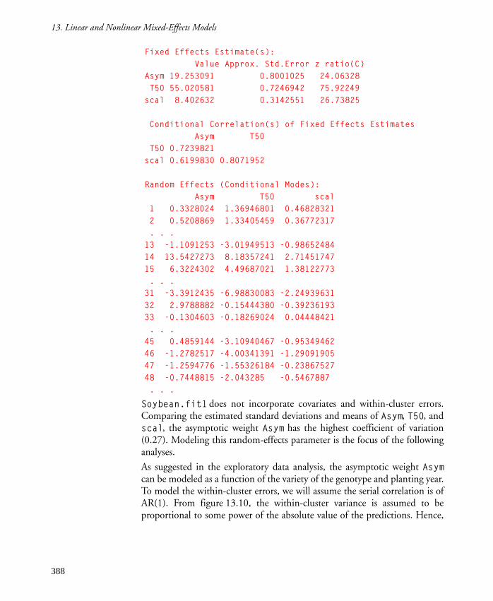
13. Linear and Nonlinear Mixed-Effects Models
Fixed Effects Estimate(s):
Value Approx. Std.Error z ratio(C)
Asym 19.253091 0.8001025 24.06328
T50 55.020581 0.7246942 75.92249
scal 8.402632 0.3142551 26.73825
Conditional Correlation(s) of Fixed Effects Estimates
Asym T50
T50 0.7239821
scal 0.6199830 0.8071952
Random Effects (Conditional Modes):
Asym T50 scal
1 0.3328024 1.36946801 0.46828321
2 0.5208869 1.33405459 0.36772317
. . .
13 -1.1091253 -3.01949513 -0.98652484
14 13.5427273 8.18357241 2.71451747
15 6.3224302 4.49687021 1.38122773
. . .
31 -3.3912435 -6.98830083 -2.24939631
32 2.9788882 -0.15444380 -0.39236193
33 -0.1304603 -0.18269024 0.04448421
. . .
45 0.4859144 -3.10940467 -0.95349462
46 -1.2782517 -4.00341391 -1.29091905
47 -1.2594776 -1.55326184 -0.23867527
48 -0.7448815 -2.043285 -0.5467887
. . .
Soybean.fit1 does not incorporate covariates and within-cluster errors.Comparing the estimated standard deviations and means of Asym, T50, andscal, the asymptotic weight Asym has the highest coefficient of variation(0.27). Modeling this random-effects parameter is the focus of the followinganalyses.
As suggested in the exploratory data analysis, the asymptotic weight Asymcan be modeled as a function of the variety of the genotype and planting year.To model the within-cluster errors, we will assume the serial correlation is ofAR(1). From figure 13.10, the within-cluster variance is assumed to beproportional to some power of the absolute value of the predictions. Hence,
388

Nonlinear Mixed-Effects Models
for the ith plot, the 8×8 covariance matrix σ2D in model (13.8) is now given
by at time j and between the
ith and jth measurements.
Two separate nlme calls are performed on the Soybean data below. The firstcall uses part of the assumptions in the above model. Only Variety is usedas a predictor. The serial correlation is assumed to be of AR(1) and thewithin-cluster variance is assumed to be identity, a default forvar.function in the nlme call.
In fitting the full model below with the second nlme call, the results fromSoybean.nlsList are used to derive initial estimates in the parametrizationof Asym.
> Soybean.fit2 <-
+ nlme(weight ~ logistic(time, Asym, T50, scal),
+ fixed = list(Asym ~ Variety, T50 ~ ., scal ~ .),
+ random = list(Asym ~ ., T50 ~ ., scal ~ .),
+ start = list(fixed = c(19.25309, 0,
+ 55.02058, 8.402632)),
+ serial.structure = "ar1",
+ cluster = ~ Plot, data = Soybean)
> Soybean.fit2
. . .
Standard Deviation(s) of Random Effect(s)
Asym.(Intercept) T50 scal
4.520749 4.223438 1.446683
Correlation of Random Effects
Asym.(Intercept) T50
T50 0.7216902
scal 0.6259055 0.7851180
Cluster Residual Variance: 1.110669
Serial Correlation Structure: ar1
Serial Correlation Parameter(s): -0.6164418
Fixed Effects Estimate(s):
Asym.(Intercept) Asym.Variety T50 scal
19.39241 2.208246 55.31789 8.647944
. . .
var eij( ) σ2yi j
2δ= cor eij eik,( ) ρ k j–=
389

13. Linear and Nonlinear Mixed-Effects Models
> # Get initial estimates in modeling Asym
> coef(lm(Asym ~ Variety * Year, Soybean.nlscoef))
(Intercept) Variety Year1 Year2
20.08425 2.03699 -3.785161 0.3036094
VarietyYear1 VarietyYear2
1.497311 -1.084704
> Soybean.fit3 <-
+ nlme(weight ~ logistic(time, Asym, T50, scal),
+ fixed = list(Asym ~
+ Variety * Year, T50 ~ ., scal ~ .),
+ random = list(Asym ~ ., T50 ~ ., scal ~ .),
+ start = list(fixed = c(20.08425, 2.03699,
+ -3.785161, 0.3036094, 1.497311,
+ -1.084704, 55.02058, 8.402632)),
+ serial.structure = "ar1",
+ var.function = "power",
+ cluster = ~ Plot, data = Soybean)
> Soybean.fit3
. . .
Standard Deviation(s) of Random Effect(s)
Asym.(Intercept) T50 scal
1.11527 1.531973 0.1430054
Correlation of Random Effects
Asym.(Intercept) T50
T50 0.9731252
scal 0.9591480 0.9975064
Cluster Residual Variance: 0.05957224
Serial Correlation Structure: ar1
Serial Correlation Parameter(s): 0.1874778
Variance Function: power
Variance Function Parameter(s): 0.9225696
Fixed Effects Estimate(s):
Asym.(Intercept) Asym.Variety Asym.Year1 Asym.Year2
17.53656 2.504791 -2.771701 1.21122
Asym.VarietyYear1 Asym.VarietyYear2 T50
1.264881 -0.3621853 52.22499
scal
7.603832
. . .
390

Nonlinear Mixed-Effects Models
> anova(Soybean.fit1,Soybean.fit2,Soybean.fit3)
. . .
Model Df AIC BIC Loglik Test
Soybean.fit1 1 10 1499.7 1539.9 -739.84
Soybean.fit2 2 12 1404.6 1452.9 -690.30 1 vs. 2
Soybean.fit3 3 17 679.9 748.2 -322.93 2 vs. 3
Lik.Ratio P value
Soybean.fit1
Soybean.fit2 99.08 0
Soybean.fit3 734.74 0
The anova function is used to compare these fits. The progress in loglikelihood, AIC, and BIC is tremendous. Figure 13.18 shows the residualsplots. No patterns are seen in the standardized residuals, even though theproblematic plots 14, 32, and 46 for the nlsList calls are included in theseanalyses. After adjustment of random effects and within-cluster errors, theirrandom effects are derived. Their standardized residuals are within (-1.5,1.5)
Figure 13.18: The residuals plots.
oooo o
oo
oo o
oooo o
oo
o o
ooo o oo
o
oo o
ooo o oo
o
o o o
ooo oo o
o
o
ooo oo o
oo
oo
ooo oo o
o
o o
ooo o oo
oo
o o
ooo oo
oo
o o o
ooo oo
oo
o o
o
ooo o oo
oo
oo
ooo oo
o o
o o
o
ooo o oo
oo o o
ooo o oo
o
oo
o
ooo o oo
oo
oo
ooo o o o
oo
oo
oooo oo
o o
oooo oo
o o
oooo oo
o
o
oooo oo
o o
ooooo
oo o
oooo oo o
o
oooo oo
oo
ooooo
o oo
ooo o o
o
oo
ooo o o
o
o
o
ooo oo
o
o o
ooo o oo
oo
ooo o oo
oo
ooo oo
o
oo
oooo o
oo o
ooo o o
o
o
o
ooo o o
oo
o
ooo o oo
o
o
ooo oo o
o
o
ooo o oo
o
o
ooo oo
o
oo
oooo o
o
oo
ooo o oo
oo
ooo oo o
oo
oooo o
o
o o
ooo o oo
o
o
oooo o
o
o o
oooo o o
o
o
oooo o
o
o o
oooo o
o
oo
ooo oo
oo
o
ooo oo o
o o
Fitted Values
Obs
erve
d V
alue
s
0 5 10 15 20
05
1525
ooo
o
o oo
o o oooo
o
o oo
o oooo
oo
o o
o o o
ooo
oo o
o
oo
oooo o
o
o o
o
ooo o
o
o oo
oo
ooo
oo
oo
o oooo
o oo
o oo o
ooo o
oo
o oo o
ooo
o o oo
o
o
o
ooo o
o oo o
oooo
o
oo
o
oo
o
ooo
oo
o o o oo o
ooo
oo o o
o
o
o
oooo o o o o
oo
oo
oo
o
o
o oo
o
ooo
oo
o
oo
ooo
o
oo o o
o
ooo o
o
o
o
ooo
o
o
oo o
oooo
o
oo
o
oooo
o
oo
oo
ooo
o
oo
oooo
o oo
oo
ooo
o
oo
oo
o
oo
o
o o o
o
oo
o
oo
oo o
ooo o oo
o o
o
oo
o o
o
o
ooo
o
o
o
o oooo
o
o
o
oo
oo
oo
oo
o
o
oooo
o
o
o
oo
ooo
o
o o ooo
oo o o
o o
o
o
o
o
o
oo o
o
oo
o
oo o o o
o
oo
o
o oo o
o
o
o
o o o
o o
o
oo
o o
o
o oo
oo o
oo
ooo
oo
o
o o o
oo
o
o
o
oo
o oo
o
oo
o
o
oo
oo
oo
o o
oo
o
o
o
o
oo
o
oo
oo
o
o
oo
oo
oo
o
o
o
oo
Fitted Values
Res
idua
ls0 5 10 15 20
-20
12
34
-20
12
34
1 2 3 4 5 6 7 8 9101112131415161718192021222324252627282930313233343536373839404142434445464748
Plot
Res
idua
ls
391

13. Linear and Nonlinear Mixed-Effects Models
except for three with values around 2.5. The variety of the genotype and theyear of planting have large impacts on the limiting leaf weight. Theexperimental strain gains 2.5 grams in the limit.
> par(mfrow = c(2,2))
> plot(Soybean.fit3, option="s")
> summary(Soybean.fit3)
. . .
Fixed Effects Estimate(s):
Value Approx. Std.Error
Asym.(Intercept) 17.5365613 0.4638525
Asym.Variety 2.5047905 0.2469177
Asym.Year1 -2.7717008 0.2829921
Asym.Year2 1.2112198 0.1864453
Asym.VarietyYear1 1.2648812 0.2776887
Asym.VarietyYear2 -0.3621853 0.1844127
T50 52.2249943 0.5073733
scal 7.6038318 0.1027588
z ratio(C)
Asym.(Intercept) 37.806334
Asym.Variety 10.144233
Asym.Year1 -9.794270
Asym.Year2 6.496381
Asym.VarietyYear1 4.555032
Asym.VarietyYear2 -1.963994
T50 102.932085
scal 73.996904
. . .
Random Effects (Conditional Modes):
Asym.(Intercept) T50 scal
. . .
14 0.049307561 0.018802336 0.0008801504
. . .
32 0.746219856 1.028182060 0.0951769261
. . .
46 -0.581105585 -0.801146841 -0.0740665473
47 -0.214035251 -0.252438575 -0.0225885040
48 -0.5266585 -0.7154175 -0.06597178
392

Nonlinear Mixed-Effects Models
Standardized Population-Average Residuals:
Min Q1 Med Q3 Max
-2.462553 -0.6578548 -0.1209506 0.5526576 4.05955
393

13. Linear and Nonlinear Mixed-Effects Models
394

NONLINEAR MODELS 1414.1 Optimization Functions 397
Finding Roots 397
Finding Local Maxima and Minima of Univariate Functions 399
Finding Maxima and Minima of Multivariate Functions 400
Solving Nonnegative Least Squares Problems 404
Solving Nonlinear Least Squares Problems 406
14.2 Examples of Nonlinear Models 408
Maximum Likelihood Estimation 408
Nonlinear Regression 411
14.3 Inference for Nonlinear Models 412
The Fitting Algorithms 412
Specifying Models 413
Parametrized Data Frames 414
Derivatives 416
Fitting Models 420
Profiling the Objective Function 428
395

14. Nonlinear Models
396
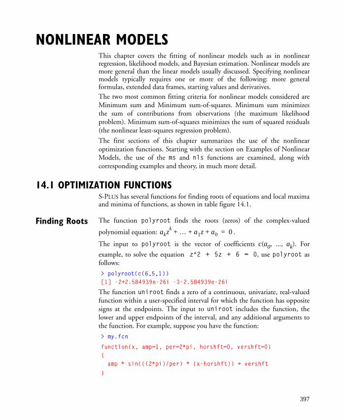
NONLINEAR MODELS 14This chapter covers the fitting of nonlinear models such as in nonlinearregression, likelihood models, and Bayesian estimation. Nonlinear models aremore general than the linear models usually discussed. Specifying nonlinearmodels typically requires one or more of the following: more generalformulas, extended data frames, starting values and derivatives.
The two most common fitting criteria for nonlinear models considered areMinimum sum and Minimum sum-of-squares. Minimum sum minimizesthe sum of contributions from observations (the maximum likelihoodproblem). Minimum sum-of-squares minimizes the sum of squared residuals(the nonlinear least-squares regression problem).
The first sections of this chapter summarizes the use of the nonlinearoptimization functions. Starting with the section on Examples of NonlinearModels, the use of the ms and nls functions are examined, along withcorresponding examples and theory, in much more detail.
14.1 OPTIMIZATION FUNCTIONSS-PLUS has several functions for finding roots of equations and local maximaand minima of functions, as shown in table figure 14.1.
Finding Roots The function polyroot finds the roots (zeros) of the complex-valued
polynomial equation: .
The input to polyroot is the vector of coefficients c(a0, ..., ak). For
example, to solve the equation z^2 + 5z + 6 = 0, use polyroot asfollows:
> polyroot(c(6,5,1))
[1] -2+2.584939e-26i -3-2.584939e-26i
The function uniroot finds a zero of a continuous, univariate, real-valuedfunction within a user-specified interval for which the function has oppositesigns at the endpoints. The input to uniroot includes the function, thelower and upper endpoints of the interval, and any additional arguments tothe function. For example, suppose you have the function:
> my.fcn
function(x, amp=1, per=2*pi, horshft=0, vershft=0)
{
amp * sin(((2*pi)/per) * (x-horshft)) + vershft
}
akzk … a1z a0+ + + 0=
397

14. Nonlinear Models
This is the sine function with amplitude abs(amp), period abs(per),horizontal (phase) shift horshft and vertical shift vershft. To find a rootof the function my.fcn in the interval [π/2, 3π/2] using its defaultarguments, type:
> uniroot(my.fcn, interval = c(pi/2, 3*pi/2))
$root
[1] 3.141593
. . .
To find a root of my.fcn in the interval [π/4, 3π/4] with the period set to π,type:
Table 14.1: The range of S-PLUS functions for finding roots, maxima and minima.
Function Description
polyroot Finds the roots of a complex polynomial equation.
uniroot Finds the root of a univariate real-valued function in a user-supplied interval.
peaks Finds local maxima in a set of discrete points.
optimize Approximates a local optimum of a continuous univariate function within agiven interval.
ms Finds a local minimum of a multivariate function.
nlmin Finds a local minimum of a nonlinear function using a general quasi-Newtonoptimizer.
nlminb Local minimizer for smooth nonlinear functions subject to bound-con-strained parameters.
nls Finds a local minimum of the sums of squares of one or more multivariatefunctions.
nlregb Local minimizer for sums of squares of nonlinear functions subject to bound-constrained parameters.
nnls Finds least-squares solution subject to the constraint that the coefficients benonnegative.
398

Optimization Functions
> uniroot(my.fcn, interval = c(pi/4, 3*pi/4), per=pi)
$root:
[1] 1.570796
. . .
> pi/2
[1] 1.570796
See the help file for uniroot for information on other arguments to thisfunction.
Finding Local
Maxima and
Minima of
Univariate
Functions
The peaks function takes a data object x and returns an object of the sametype with logical values: T if a point is a local maximum, otherwise F:
> peaks(corn.rain)
1890: F T F F F F T F T F T F T F F F F T F F F F T F F T F
1917: T F F F T F F T F T F
Use peaks on the data object -x to find local minima:
> peaks(-corn.rain)
1890: F F F F T F F F F F F T F F F T F F F F F T F T F F T
1917: F T F F F T F F T F F
To find a local optimum (maximum or minimum) of a continuous univariatefunction within a particular interval, use the optimize function. The inputto optimize includes the function to optimize, the lower and upperendpoints of the interval, which optimum to look for (maximum versusminimum) and any additional arguments to the function.
> optimize(my.fcn, c(0, pi), maximum=T)
$maximum:
[1] 1.570799
$objective:
[1] -1
$nf:
[1] 10
$interval:
[1] 1.570759 1.570840
. . .
399

14. Nonlinear Models
> pi/2
[1] 1.570799
> optimize(my.fcn, c(0, pi), maximum=F, per = pi)
$minimum:
[1] 2.356196
$objective:
[1] -1
$nf:
[1] 9
$interval:
[1] 2.356155 2.356236
. . .
> 3*pi/4
[1] 2.356194
See the help file for optimize for information on other arguments to thisfunction.
Finding
Maxima and
Minima of
Multivariate
Functions
S-PLUS has two functions to find the local minimum of a multivariatefunction: nlminb (Nonlinear Minimization with Box Constraints) and ms(Minimize Sums).
The two required arguments to nlminb are objective (the function f tominimize) and start (a vector of starting values for the minimization). Thefunction f must take as its first argument a vector of parameters over whichthe minimization is carried out. By default, there are no boundary constraintson the parameters. The nlminb function, however, also takes the optionalarguments lower and upper that specify the bounds on the parameters.(Other arguments to f can be passed in the call to nlminb.)
1. Example: Using nlminb to find a local minimum.
> my.multvar.fcn
function(xvec, ctr = rep(0, length(xvec)))
{
if(length(xvec) != length(ctr))
stop("lengths of xvec and ctr do not match")
sum((xvec - ctr)^2)
}
400

Optimization Functions
> nlminb(start = c(0,0), objective = my.multvar.fcn,
+ ctr = c(1,2))
$parameters:
[1] 1 2
$objective:
[1] 3.019858e-30
$message:
[1] "ABSOLUTE FUNCTION CONVERGENCE"
. . .
To find a local maximum of f, use nlminb on -f. Since unary minus cannotbe performed on a function, you must define a new function that returns -1times the value of the function you want to maximize:
2. Example: Using nlminb to find a local maximum.
> fcn.to.maximize
function(xvec)
{
- xvec[1]^2 + 2 * xvec[1] - xvec[2]^2 + 20 * xvec[2] + 40
}
> fcn.to.minimize
function(xvec)
{
- fcn.to.maximize(xvec)
}
> nlminb(start = c(0, 0), objective = fcn.to.minimize)
$parameters:
[1] 1 10
$objective:
[1] -141
$message:
[1] "RELATIVE FUNCTION CONVERGENCE"
. . .
See the help file for nlminb for information on other arguments to thisfunction. To find the local minimum of a multivariate function subject toconstraints, use nlminb with the lower and/or upper arguments.
401
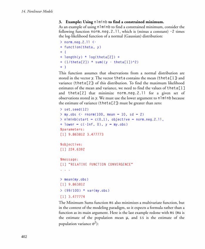
14. Nonlinear Models
3. Example: Using nlminb to find a constrained minimum.As an example of using nlminb to find a constrained minimum, consider thefollowing function norm.neg.2.ll, which is (minus a constant) -2 timesthe log-likelihood function of a normal (Gaussian) distribution:
> norm.neg.2.ll <-
+ function(theta, y)
+ {
+ length(y) * log(theta[2]) +
+ (1/theta[2]) * sum((y - theta[1])^2)
+ }
This function assumes that observations from a normal distribution arestored in the vector y. The vector theta contains the mean (theta[1]) andvariance (theta[2]) of this distribution. To find the maximum likelihoodestimates of the mean and variance, we need to find the values of theta[1]and theta[2] that minimize norm.neg.2.ll for a given set ofobservations stored in y. We must use the lower argument to nlminb becausethe estimate of variance (theta[2]) must be greater than zero:
> set.seed(12)
> my.obs <- rnorm(100, mean = 10, sd = 2)
> nlminb(start = c(0,1), objective = norm.neg.2.ll,
+ lower = c(-Inf, 0), y = my.obs)
$parameters:
[1] 9.863812 3.477773
$objective:
[1] 224.6392
$message:
[1] "RELATIVE FUNCTION CONVERGENCE"
. . .
> mean(my.obs)
[1] 9.863812
> (99/100) * var(my.obs)
[1] 3.477774
The Minimum Sums function ms also minimizes a multivariate function, butin the context of the modeling paradigm, so it expects a formula rather than afunction as its main argument. Here is the last example redone with ms (mu isthe estimate of the population mean µ, and ss is the estimate of the
population variance σ2):
402

Optimization Functions
4. Example: Using ms.
> ms( ~length(y) * log(ss) + (1/ss) * sum((y - mu)^2),
+ data = data.frame(y = my.obs),
+ start = list(mu = 0, ss = 1))
value: 224.6392
parameters:
mu ss
9.863813 3.477776
formula: ~length(y) * log(ss) + (1/ss) * sum((y-mu)^2)
1 observations
call: ms(formula = ~length(y) * log(ss) + (1/ss) *
sum((y - mu)^2),
data = data.frame(y=my.obs), start=list(mu=0, ss=1))
5. Example: Using ms with several observations.
> ms( ~log(ss) + (1/ss) * (y - mu)^2,
+ data = data.frame(y = my.obs),
+ start = list(mu = 0, ss = 1))
value: 224.6392
parameters:
mu ss
9.863813 3.477776
formula: ~log(ss) + (1/ss) * (y - mu)^2
100 observations
call: ms(formula = ~log(ss) + (1/ss) * (y - mu)^2,
data = data.frame(y=my.obs), start=list(mu=0,ss=1))
Hint: The ms function does not do minimization subject to constraints on the parameters.
If there are multiple solutions to your minimization problem, you may not get the answer youwant using ms. In the above example, the ms function tells us we have �1 observations" becausethe whole vector y was used at once in the formula. The Minimum Sum function minimizes thesum of contributions to the formula, so we could have gotten the same estimates mu and ss withthe formula shown in example 5.
403

14. Nonlinear Models
If the function you are trying to minimize is fairly complicated, then it isusually easier to write a function to supply as the formula:
6. Example: Using ms with a formula function.
> ms( ~norm.neg.2.ll(theta,y), data=data.frame(y=my.obs),
+ start = list(theta = c(0,1)))
value: 224.6392
parameters:
theta1 theta2
9.863813 3.477776
formula: ~norm.neg.2.ll(theta, y)
1 observations
call: ms(formula = ~norm.neg.2.ll(theta, y), data =
data.frame(y = my.obs),
start = list(theta = c(0, 1)))
Solving
Nonnegative
Least Squares
Problems
Given an m × n matrix A and a vector b of length m, the linear nonnegativeleast squares problem is to find the vector x of length n that minimizes
, subject to the constraint that for i in 1, ..., n.
To solve nonnegative least squares problems in S-PLUS, use the nnls.fitfunction. For example, consider the following fit using the stack data:
$coefficients
Air Flow Water Temp Acid Conc.
0.2858057 0.05715152 0
$residuals:
[1] 17.59245246 12.59245246 14.13578403
[4] 8.90840973 -0.97728723 -1.03443875
[7] -0.09159027 0.90840973 -2.89121593
[10] -3.60545832 -3.60545832 -4.54830680
[13] -6.60545832 -5.66260984 -7.31901267
[16] -8.31901267 -7.37616419 -7.37616419
[19] -6.43331572 -2.14814995 -6.14942983
$dual:
Air Flow Water Temp Acid Conc.
3.637979e-12 5.400125e-13 -1438.359
Ax b– xi 0≥
404

Optimization Functions
$rkappa:
final minimum
0.02488167 0.02488167
$call:
nnls.fit(x = stack.x, y = stack.loss)
You can also use nlregb to solve the nonnegative least squares problem,since the nonnegativity constraint is just a simple box constraint. To pose theproblem to nlregb, define two functions (lin.res and lin.jac) of theform f(x,params), to represent the residual function and the Jacobian ofthe residual function, respectively:
> lin.res <- function(x, b, A) A%*% x - b
> lin.jac <- function(x, A) A
> nlregb(n = length(stack.loss), start = rnorm(3),
+ res = lin.res, jac = lin.jac, lower = 0,
+ A = stack.x, b = stack.loss)
$parameters:
[1] 0.28580571 0.05715152 0.00000000
$objective:
[1] 1196.252
. . .
Generally, nnls.fit should be preferred to nlregb for reasons of efficiency,since nlregb is primarily designed for nonlinear problems. However,nlregb can solve degenerate problems that can not be handled bynnls.fit. You may also want to compare the results of nnls.fit withthose of lm. Remember that lm requires a formula, and also that it fits anintercept term by default (which nnls.fit does not). Keeping this in mind,you can construct the comparable call to lm as follows:
> lm(stack.loss ~ stack.x - 1)
Call:
lm(formula = stack.loss ~ stack.x - 1)
Coefficients:
stack.xAir Flow stack.xWater Temp
0.7967652 1.111422 -0.6249933
Degrees of freedom: 21 total; 18 residual
Residual standard error: 4.063987
405

14. Nonlinear Models
For the stack loss data, the results of the constrained optimization methodsnnls.fit and nlregb agree completely. The linear model produced by lmincludes a negative coefficient.
You can use nnls.fit to solve the weighted nonnegative least squaresproblem by providing a vector of weights as the weights argument. Theweights used by lm are the square roots of the weights used by nnls.fit;you must keep this in mind if you are trying to solve a problem using bothfunctions.
Solving
Nonlinear
Least Squares
Problems
Two functions, nls and nlregb, are available for solving the specialminimization problem of nonlinear least squares. The function nls is usedin the context of the modeling paradigm, so it expects a formula rather than afunction as its main argument. The function nlregb expects a functionrather than a formula (the argument name is residuals), and, unlike nls,it can perform the minimization subject to constraints on the parameters.
1. Example: Using nls. In this example, we create 100 observations where the underlying signal is asine function with an amplitude of 4 and a horizontal (phase) shift of π.Noise is added in the form of normal (Gaussian) random numbers. We thenuse the nls function to estimate the true values of amplitude and horizontalshift.
> set.seed(20)
> noise <- rnorm(100, sd = 0.5)
> x <- seq(0, 2*pi, length = 100)
> my.nl.obs <- 4 * sin(x - pi) + noise
> plot(x, my.nl.obs)
> nls(y ~ amp * sin(x - horshft),
+ data = data.frame(y = my.nl.obs, x = x),
+ start = list(amp = 1, horshft = 0))
Residual sum of squares : 20.25668
parameters:
amp horshft
-4.112227 0.01059317
formula: y ~ amp * sin(x - horshft)
100 observations
The above example illustrates the importance of finding appropriate startingvalues. The nls function returns an estimate of amp close to -4 and anestimate of horshft close to 0 because of the cyclical nature of the sinefunction: sin(x - pi) = -sin(x). If we start with initial estimates ofamp and horshft closer to their true values, nls gives us the estimates wewant.
406

Optimization Functions
2. Example: Using nls with better starting values.
> nls(y ~ amp * sin(x - horshft),
+ data = data.frame(y = my.nl.obs, x = x),
+ start = list(amp = 3, horshft = pi/2))
Residual sum of squares : 20.25668
parameters:
amp horshft
4.112227 -3.131
formula: y ~ amp * sin(x - horshft)
100 observations
We could use the nlregb function to redo the above example, and specifythat the value of amp must be greater than 0:
3. Example: Creating my.new.func and using nlregb.
> my.new.fcn
function(param, x, y)
{
amp <- param[1]
horshft <- param[2]
y - amp * sin(x - horshft)
}
> nlregb(n = 100, start = c(3,pi/2),
+ residuals = my.new.fcn,
+ lower = c(0, -Inf), x = x, y = my.nl.obs)
$parameters:
[1] 4.112227 3.152186
$objective:
[1] 20.25668
$message:
[1] "BOTH X AND RELATIVE FUNCTION CONVERGENCE"
$grad.norm:
[1] 5.960581e-09
407

14. Nonlinear Models
14.2 EXAMPLES OF NONLINEAR MODELS
Maximum
Likelihood
Estimation
Parameters are estimated by maximizing the likelihood function. Suppose nindependent observations are distributed with probability densities pi(θ)=
p(yi;θ) where θ is a vector of parameters. The likelihood function is defined
as:
The problem is to find the estimate of that maximizes the likelihood
function for the observed data. Maximizing the likelihood is equivalent tominimizing the negative of the log-likelihood:
Example One:
Ping-Pong
Each member of the U.S. Table Tennis Association is assigned a rating basedon the member�s performance in tournaments. Winning a match boosts thewinner�s rating and lowers the loser�s rating some number of pointsdepending on the current ratings of the two players. Using this data, twoquestions we might like to ask are:
1. Do players with a higher rating tend to win over players with a lowerrating?
2. Does a larger difference in rating imply that the higher-rated playeris more likely to win?
Assuming a logistic distribution in which log(p/(1-p)) is proportional tothe difference in rating between the winner and loser and the average ratingof the two players:
where Di = Wi - Li is the difference in rating between the winner andloser and Ri = 1/2(Wi + Li) is the average rating for the two players.
(14.1)
(14.2)
L y θ;( ) pi θ( )i 1=
n
∏=
θ
l θ( ) L y θ;( )( )log– pi θ( )( )log–( )i 1=
n
∑= =
(14.3)pie
Di α Ri β+
1 eDi α Ri β+
+
------------------------------=
408

Examples of Nonlinear Models
To fit the model, we need to find α and β which minimize the negative log-likelihood:
Example Two:
Wave-Soldering
Skips
In a 1988 AT&T wave-soldering experiment several factors were varied:
The results of the experiment gave the number of visible soldering skips(faults) on a board. Physical theory and intuition suggest a model in whichthe process is in one of two states:
1. a �perfect� state where no defects occur.
2. an �imperfect� state where there may or may not be defects.
Both the probability of being in the imperfect state and the distribution ofskips in that state depend on the factors in the experiment. Assume that some�stress�, S, induces the process to be in the imperfect state and also increasesthe tendency to generate skips when in the imperfect state.
Assume S depends linearly on the levels of the factors, xj, j=1,...,p:
where β is the vector of parameters to be estimated.
(14.4)pi( )log–( )∑ D– iα Riβ 1 eDi α Ri β+
+( )log+– ∑=
Factor Description
opening amount of clearance around the mounting pad
solder amount of solder
mask type and thickness of the material used for the solder mask
padtype the geometry and size of the mounting pad
panel each board was divided into three panels, with three runs on a board
(14.5)Si xij βj
j 1=
p
∑=
409

14. Nonlinear Models
Assume the probability Pi of being in the imperfect state is monotonically
related to the stress by a logistic distribution:
As the stress increases, the above function approaches 1.
Given that the process is in an imperfect state, assume the probability of ki
skips is modeled by the Poisson distribution with mean λi:
The probability of zero skips is the probability of being in the perfect stateplus the probability of being in the imperfect state and having zero skips. Theprobability of one or more skips is the probability of being in the imperfectstate and having one or more skips. Mathematically the probabilities may bewritten as:
The mean skips in the imperfect state is always positive and modeled in terms
of the stress by: . The parameters, τ and β, can be estimated by
minimizing the negative log-likelihood. The ith element of the negative log-likelihood can be written to within constants as:
The model depicted above does not reduce to any simple linear model.
(14.6)
(14.7)
(14.8)
Pi1
1 eτ–( )Si+
-----------------------=
P ki( ) eλ– i λ
kii
ki!-------⋅=
P y yi=( )
eτ–( )Si
1 eτ–( )Si+
----------------------- eλ– i
1 eτ–( )Si+
-----------------------+ if yi 0=
1
1 eτ–( )Si+
-----------------------eλ– i λ
yii
yi!------- if yi 0>
=
λi eSi=
(14.9)l i β τ,( ) 1 eτ–( )Si+( )log
eτ–( )Si e
e–Si
+ log if yi 0=
yiSi e–Si if yi 0>
–=
410

Examples of Nonlinear Models
Nonlinear
Regression
Parameters are estimated by minimizing the sum of squared residuals.Suppose n independent observations y can be modeled as a nonlinearparametric function f of a vector x of predictor variables and a vector ofparameters, β.
where the errors, ε, are assumed normally distributed. The nonlinear least-
squares problem finds parameter estimates which minimize:
Example Three:
Puromycin
A biochemical experiment measured reaction velocity in cells with andwithout treatment by Puromycin. There are three variables in thePuromycin data frame.
Assume a Michaelis-Menten relationship between velocity andconcentration:
where V is the velocity, c is the enzyme concentration, Vmax is a parameter
representing the asymptotic velocity as c �> ∞, K is the Michaelis parameter,and ε is experimental error. Assuming the treatment with the drug wouldchange Vmax but not K, the optimization function is:
where I{treated} is the function indicating if the cell was treated with
Puromycin.
(14.10)
y f x β;( ) ε+=
β
yi f x β;( )–( )2
i 1=
n
∑
Variable Description
conc the substrate concentration
vel the reaction velocity
state indicator of treated or untreated
(14.11)
(14.12)
VVmaxc
K c+-------------- ε+=
S Vmax K,( ) ViVmax ∆VmaxI treated{ } state( )+( )ci
K ci+-----------------------------------------------------------------------------------–
2
∑=
411

14. Nonlinear Models
14.3 INFERENCE FOR NONLINEAR MODELS
Likelihood
Models
With likelihood models distributional results are asymptotic. Maximumlikelihood estimates tend toward a normal distribution with a mean equal tothe true parameter, and a variance matrix given by the inverse of theinformation matrix, the negative of the second derivatives of the log-likelihood.
Least-Squares
Models
In least-squares models approximations to quantities such as standard errorsor correlations of parameter estimates are used. The approximation proceedsas follows:
1. Replace the nonlinear model with its linear Taylor seriesapproximation at the parameter estimates.
2. Use the methods for linear statistical inference on theapproximation.
Consequently, the nonlinear inference results are called linear approximationresults.
The Fitting
Algorithms
Minimum-Sum
Algorithm
This section deals with the general optimization of an objective functionmodeled as a sum. The algorithm is a version of Newton�s method based on aquadratic approximation of the objective function. If both first and secondderivatives are supplied, the approximation is a local one using thederivatives. If no derivatives or only the first derivative are supplied, thealgorithm approximates the second derivative information. It does this in away specifically designed for minimization.
The algorithm actually used is taken from the PORT subroutine librarywhich evolved from the published algorithm by Gay (1983). Two keyfeatures of this algorithm are:
1. A quasi-Newton approximation for second derivatives.
2. A �trust region� approach controlling the size of the region in whichthe quadratic approximation is believed to be accurate.
The algorithm is capable of working with user models specifying 0, 1, or 2orders of derivatives.
412

Inference for Nonlinear Models
Nonlinear Least-
Squares
Algorithm
The Gauss-Newton algorithm is used with a step factor to ensure that thesum of squares decreases at each iteration. A line-search method is used, asopposed to the trust region employed in the minimum-sum algorithm. Thestep direction is determined by a quadratic model. The algorithm proceeds asfollows:
1. The residuals are calculated, and the gradient is calculated orapproximated (depending on the data), at the current parametervalues.
2. A linear least-squares fit of the residual on the gradient gives theparameter increment.
3. If applying the full parameter increment increases the sum-of-squares rather than decreasing it, the length of the increment issuccessively halved until the sum-of-squares is decreased.
4. The step factor is retained between iterations and started at min{2*(previous step factor), 1}
If the gradient is not specified analytically, it is calculated using finitedifferences with forward differencing. For partially linear models, theincrement is calculated using the Golub-Pereyra method (Golub and Pereyra,1973) as implemented by Bates and Lindstrom (1986).
Specifying
Models
Nonlinear models typically require specifying more details than models ofother types. The information typically required to fit a nonlinear model,using the S-PLUS functions ms or nls is:
1. a formula
2. data
3. starting values
Formulas For nonlinear models a formula is an S-PLUS expression involving data,parameters in the model, and any other relevant quantities. The parametersmust be specified in the formula because there is no assumption about wherethey are to be placed (as in linear models, for example). Formulas are typicallyspecified differently depending on whether you have a minimum-sumproblem or nonlinear least-squares problem.
In the puromycin example you would specify a formula for the simple model(described in equation 14.11) by: vel ~ Vm*conc / (K + conc)
The parameters Vm and K are specified along with the data vel and conc.Since there is no explicit response for minimum-sum models (e.g. likelihoodmodels), it is left off in the formula.
413

14. Nonlinear Models
In the ping-pong example (ignoring the average rating effect), the formula for(equation 14.4) is:
~- DV * alpha + log( 1 + exp( DV * alpha ) )
where DV is a variable in the data and alpha is the parameter to fit. Note thatthe model here is based only on the difference in ratings, ignoring for themoment the average rating.
Simplifying
Formulas
Some models can be organized as a simple expression involving one or moreS-PLUS functions that do all the work. Note that DV*alpha occurs twice inthe formula for the ping-pong model. You can write a general function forthe log-likelihood in terms of DV*alpha.
> lprob <- function(lp) log(1 + exp(lp)) - lp
Recall that lp is the linear predictor for the GLM. A simpler expression forthe model is now:
~ lprob( DV * alpha )
Having lprob now makes it easy to add additional terms or parameters.
Implications of
the Formulas
For nonlinear least-squares formulas the response on the left of ~ and thepredictor on the right must evaluate to numeric vectors of the same length.The fitting algorithm tries to estimate parameters to minimize the sum ofsquared differences between response and prediction. If the response is leftout the formula is interpreted as a residual vector.
For Minimum-Sum formula, the right of ~ must evaluate to a numericvector. The fitting algorithm tries to estimate parameters to minimize thesum of this �predictor� vector. The concept here is linked to maximum-likelihood models. The computational form does not depend on an MLEconcept. The elements of the vector may be anything and there need not bemore than one.
The evaluated formulas can include derivatives with respect to theparameters. The derivatives are supplied as attributes to the vector that resultswhen the predictor side of the formula is evaluated. When explicit derivativesare not supplied, the algorithms use numeric approximations.
Parametrized
Data Frames
Relevant data for nonlinear modeling includes:
� variables
� initial estimates of parameters
� fixed values occurring in a model formula
414

Inference for Nonlinear Models
Parametrized data frames allow you to �attach� relevant data to a data framewhen the data doesn�t occupy an entire column. Information is attached as a"parameter" attribute of the data frame. The parameter function returnsor modifies the entire list of parameters and is analogous to the attributesfunction. Similarly the param function returns or modifies one parameter ata time and is analogous to the attr function. You could supply values for Vmand K to the Puromycin data frame with:
> parameters(Puromycin) <- list(Vm = 200, K = 0.1)
The parameter values can be retrieved with
> parameters(Puromycin)
$Vm:
[1] 200
$K:
[1] 0.1
The class of Puromycin is now:
> class(Puromycin)
[1] "pframe" "data.frame"
Now, when Puromycin is attached, the parameters Vm and K are availablewhen referred to in formulas.
Starting Values;
Identifying
Parameters
Before the formulas can be evaluated, the fitting functions must know whichnames in the formula are parameters to be estimated and must have startingvalues for these parameters. The fitting functions determine this in thefollowing way:
1. If the start argument is supplied, its names are the names of theparameters to be estimated, and its values are the correspondingstarting values.
2. If start is missing, the parameters attribute of the data argumentdefines the parameter names and values
Hint: explicitly use the start argument to name and initialize parameters.
You can easily see what the starting values are in the call component of the fit and you canarrange to keep particular parameters constant when that makes sense.
415

14. Nonlinear Models
Derivatives Supplying derivatives of the predictor side of the formula with respect to theparameters along with the formula can reduce the number of iterations (sospeed up the computations), increase numerical accuracy and improve thechance of convergence. In general derivatives should be used wheneverpossible.
The fitting algorithms can use both first (the gradient) and second derivatives(the Hessian). The derivatives are supplied to the fitting functions asattributes to the formula. Recall that evaluating the formula gives a vector ofn values. Evaluating the first derivative expression should give n values foreach of the p parameters, that is an n × p matrix. Evaluating the secondderivative expression should give n values for each of the p × p partialderivatives, that is an n × p × p array.
First Derivatives The negative log-likelihood for the simple ping-pong model is:
Differentiating with respect to α and simplifying gives the gradient:
The gradient is supplied to the fitting function as the "gradient" attributeof the formula:
> form.pp <- ~log(1 + exp( DV*alpha ) ) - DV*alpha > attr(form.pp, "gradient") <-
+ ~ -DV / ( 1 + exp( DV*alpha ) )
> form.pp
~ log(1 + exp(DV * alpha)) - DV * alpha
> attr(form.pp,"gradient")
~ - DV/(1 + exp(DV * alpha))
When a function is used to simplify a formula, build the gradient into thefunction. The lprob function is used to simplify the formula expression to~lprob(DV*alpha).
> lprob
function(lp)
log(1 + exp(lp)) - lp
(14.13)
(14.14)
l α( ) 1 eDi α+( )log Diα–[ ]∑=
∂l∂α-------
Di–
1 eDi α+( )
------------------------∑=
416

Inference for Nonlinear Models
An improved version of lprob adds the gradient.
> lprob2
function(lp, X)
{
elp <- exp(lp)
z <- 1 + elp
value <- log(z) - lp
attr(value, "gradient") <- -X/z
value
}
Note lp is again the linear predictor and X is the data in the linear predictor.With the gradient built into the function you don�t need to add it as anattribute to the formula; it is already an attribute to the object hence used inthe formula.
Second
Derivatives
The second derivatives may be added as the "hessian" attribute of theformula. In the ping-pong example the second derivative of the negative log-likelihood with respect to α is:
The lprob2 function is now modified to add the Hessian as follows. TheHessian is added in a general enough form to allow for multiple predictors.
> lprob3
function(lp, X)
{
elp <- exp(lp)
z <- 1 + elp
value <- log(z) - lp
attr(value, "gradient") <- -X/z
if(length(dx <- dim(X)) == 2)
{
n <- dx[1]; p <- dx[2]
} else
{
n <- length(X); p <- 1
}
(14.15)∂2l
∂α2---------
Di2e
Di α
1 eDi α+( )
2--------------------------∑=
417

14. Nonlinear Models
xx <- array(X, c(n, p, p))
attr(value, "hessian") <- (xx * aperm(xx, c(1, 3, 2)) *
elp)/z^2
value
}
Interesting points of the added code are:
� The second derivative computations are performed at the time of theassignment of the "hessian" attribute.
� The rest of the code (starting with if(length(...))) is to makethe Hessian general enough for multiple predictors.
� The aperm function does the equivalent of a transpose on the 2ndand 3rd dimensions to produce the proper cross products whenmultiple predictors are in the model.
Symbolic
Differentiation
A symbolic differentiation function, D, is available to aid in takingderivatives.
The function D is used primarily as a support routine to deriv.
Again referring to the ping-pong example, form contains the expression ofthe negative log-likelihood:
> form
expression(log((1 + exp(DV * alpha))) - DV * alpha)
The first derivative is computed as:
> D(form, "alpha")
(exp(DV * alpha) * DV)/(1 + exp(DV * alpha)) - DV
And the second derivative is computed as:
> D( D(form, "alpha"), "alpha")
(exp(DV * alpha) * DV * DV)/(1 + exp(DV * alpha))
- (exp(DV * alpha) * DV * (exp(DV * alpha) * DV))
/(1 + exp(DV * alpha))^2
Table 14.2: Arguments to D
Argument Purpose
expr Expression to be differentiated.
name Which parameters to differentiate with respect to.
418

Inference for Nonlinear Models
Improved
Derivatives
The deriv function takes an expression, computes a derivative, simplifiesthe result then returns an expression or function for computing the originalexpression along with its derivative(s).
Periods are used in front of created object names to avoid conflict with userchosen names. The deriv function returns an expression in the formexpected for nonlinear models.
> deriv(form,"alpha")
expression(
{
.expr1 <- DV * alpha
.expr2 <- exp(.expr1)
.expr3 <- 1 + .expr2
.value <- (log(.expr3)) - .expr1
.grad <- array(0, c(length(.value), 1), list(NULL, "alpha"))
.grad[, "alpha"] <- ((.expr2 * DV)/.expr3) - DV
attr(.value, "gradient") <- .grad
.value
})
Table 14.3: Arguments to deriv
Argument Purpose
expr Expression to be differentiated, typically a formula, inwhich case the expression returned computes the rightside of the ~ and its derivatives.
namevec Character vector of names of parameters.
function.arg Optional argument vector or prototype for a func-tion.
tag Base of the names to be given to intermediate results.Default is ".expr".
419

14. Nonlinear Models
If the function.arg argument is supplied, a function is returned.
> deriv(form,"alpha",c("DV","alpha"))
function(DV, alpha)
{ .expr1 <- DV * alpha
.expr2 <- exp(.expr1)
.expr3 <- 1 + .expr2
.value <- (log(.expr3)) - .expr1
.grad <- array(0, c(length(.value), 1), list(NULL, "alpha"))
.grad[, "alpha"] <- ((.expr2 * DV)/.expr3) - DV
attr(.value, "gradient") <- .grad
.value
}
The namevec argument can be a vector.
> deriv(vel ~ Vm * (conc/(K + conc)), c("Vm","K")) expression(
{ .expr1 <- K + conc
.expr2 <- conc/.expr1
.value <- Vm * .expr2
.grad <- array(0, c(length(.value), 2), list(NULL, c("Vm","K")))
.grad[, "Vm"] <- .expr2
.grad[, "K"] <- - (Vm * (conc/(.expr1^2)))
attr(.value, "gradient") <- .grad
.value
})
The symbolic differentiation interprets each parameter as a scalar.Generalization from scalar to vector parameters (for example, lprob2) mustbe done by hand. Use parentheses to help deriv find relevantsubexpressions. Without the redundant parentheses around conc/(K +conc) the expression deriv returns is not as simple as possible.
Fitting Models There are two different fitting functions for nonlinear models:
� ms minimizes the sum of the vector supplied as the right side of theformula.
� nls minimizes the sum of squared differences between the left andright sides of the formula.
420

Inference for Nonlinear Models
Table 14.4: Arguments to ms
Argument Purpose
formula The nonlinear model formula (without a left side).
data A data frame in which to do the computations.
start Numeric vector of initial parameter values for the iter-ation.
scale Parameter scaling.
control List of control values to be used in the iteration.
trace Indicates whether or not intermediate estimatesshould be printed.
Table 14.5: Arguments to nls
Argument Purpose
formula The nonlinear regression model as a formula.
data A data frame in which to do the computations.
start Numeric vector of initial parameter values for the iter-ation.
control List of control values to be used in the iteration.
algorithm Which algorithm to use. The default algorithm is aGauss-Newton algorithm. If algorithm = "plin-ear", the Golub-Pereyra algorithm for partially linearleast-squares models is used.
trace Indicates whether or not intermediate estimatesshould be printed.
421

14. Nonlinear Models
Fitting a Model
to the Puromycin
Data
Before fitting a model, take a look at the data displayed in figure 14.1.
> attach(Puromycin)
> plot(conc,vel,type="n")
> text(conc,vel,ifelse(state == "treated", "T","U"))
1. Estimating Starting Values
Obtain an estimate of Vmax for each group as the maximum value each group
attains.
� The treated group has a maximum of about 200.
� The untreated group has a maximum of about 160.
The value of K is the concentration at which V reaches Vmax/2, roughly 0.1
for each group.
2. A Simple Model
Start by fitting a simple model for the treated group only.
> Treated <- Puromycin[Puromycin$state == "treated",]
> Purfit.1 <- nls(vel ~ Vm*conc/(K + conc), data = Treated, + start = list(Vm = 200, K = 0.1))
Figure 14.1: vel versus conc for treated (T) and untreated (U) groups.
vel
0.0 0.2 0.4 0.6 0.8 1.0
5010
015
020
0T
T
TT
T
T
TT
TT T
T
U
U
UUU
U
UU
UU U
conc
422

Inference for Nonlinear Models
> Purfit.1
residual sum of squares: 1195.449
parameters:
Vm K
212.6836 0.06412111
12 observations
gradient.norm:
[1] 0.2781043
RELATIVE FUNCTION CONVERGENCE
formula: vel~(Vm * conc)/(K + conc)
Fit a model for the untreated group similarly but with Vm = 160.
> Purfit.2
residual sum of squares: 859.6043
parameters:
Vm K
160.28 0.04770808
11 observations
gradient.norm:
[1] 0.1389438
RELATIVE FUNCTION CONVERGENCE
formula: vel ~ (Vm * conc)/(K + conc)
423

14. Nonlinear Models
3. A More Complicated Model
Obtain summaries of the fits with the summary function:
> summary(Purfit.1)
parameters:
Value Std.Error t value
Vm 212.68362994 6.947148850 30.614520
K 0.06412111 0.008280931 7.743225
. . .
sigma: 10.93366
df:
[1] 2 10
. . .
correlation:
Vm K
Vm 1.0000000 0.7650835
K 0.7650835 1.0000000
formula:
vel ~ (Vm * conc)/(K + conc)
> summary(Purfit.2)
parameters:
Value Std.Error t value
Vm 160.27997949 6.480240801 24.733646
K 0.04770808 0.007781862 6.130677
. . .
sigma: 9.773003
df:
[1] 2 9
. . .
correlation:
Vm K
Vm 1.0000000 0.7768269
K 0.7768269 1.0000000
formula:
vel ~ (Vm * conc)/(K + conc)
424

Inference for Nonlinear Models
An approximate t-test for the difference in K between the two modelssuggests there is no difference:
> (.06412 - .04771)/sqrt(.00828^2 + .007782^2)
[1] 1.44416
The correct test of whether the Ks should be different, and is as follows:
> Purboth <- nls(vel ~ (Vm + delV*(state=="treated"))*conc/
+ (K + conc), data=Puromycin,
+ start=list(Vm=160, delV=40, K=0.05))
> summary(Purboth)
parameters:
Value Std.Error t value
Vm 166.60396617 5.807422147 28.688110
delV 42.02590886 6.272136003 6.700414
K 0.05797157 0.005910154 9.808809
. . .
sigma: 10.58511
df:
[1] 3 20
. . .
Vm delV K
Vm 1.0000000 -0.54055820 0.61128147
delV -0.5405582 1.00000000 0.06440645
K 0.6112815 0.06440645 1.00000000
formula:
vel ~ ((Vm + delV * (state == "treated")) * conc)/(K + conc)
> combinedSS <- sum(Purfit.1$res^2) + sum(Purfit.2$res^2)
> Fval <- (sum(Purboth$res^2) - combinedSS)/(combinedSS/19)
> Fval
[1] 1.718169
> 1 - pf(Fval, 1, 19)
[1] 0.2055523
Using a single K appears to be reasonable.
Fitting a Model
to the Ping-Pong
Data
The example here develops a model based only on the difference in ratings,ignoring, for the moment, the average rating. The model to fit is:
~ DV * alpha + log( 1 + exp(DV * alpha) )
425

14. Nonlinear Models
There are four stages to the development of the model.
1. Estimating Starting Values
A very crude initial estimate for alpha can be found as follows:
� Replace all the differences in ratings by , where is the mean
difference.
� For each match, the probability from the model that the winner had
a higher rating satisfies: * a = log(p/(1-p))
� Solve for α by substituting for p the observed frequency with whichthe player with the higher rating wins.
The computations in S-PLUS proceed as follows:
> param(pingpong, "p") <- 0 # make pingpong a "pframe"
> attach(pingpong,1)
> DV <- winner - loser
> p <- sum(winner > loser) /length(winner)
> p
[1] 0.8223401
> alpha <- log(p/(1-p))/mean(DV)
> alpha
[1] 0.007660995
> detach(1, save = "pingpong")
2. A Simple Model
Recall the lprob function which calculates the log-likelihood for the ping-pong problem.
> lprob
function(lp)
log(1 + exp(lp)) - lp
The model is fitted as follows:
> attach(pingpong)
> fit.alpha <- ms( ~ lprob( DV * alpha ),
+ start = list(alpha=0.0077))
d± d
d
426

Inference for Nonlinear Models
> fit.alpha
objective: 1127.635
parameters:
alpha
0.01114251
gradient:
[1] -0.0004497159
RELATIVE FUNCTION CONVERGENCE.
formula: ~ lprob(DV * alpha)
3. Adding The Gradient
To fit the model with the gradient added to the formula use lprob2.
> fit.alpha.2 <- ms( ~ lprob2( DV * alpha, DV),
+ start = list(alpha=0.0077))
> fit.alpha.2
objective: 1127.635
parameters:
alpha
0.01114251
gradient:
alpha
2.938858e-07
RELATIVE FUNCTION CONVERGENCE.
formula: ~ lprob2(DV * alpha, DV)
Even for this simple problem, providing the derivative has decreased thecomputation time by 20%.
4. Adding The Hessian
To fit the model with the gradient and the Hessian added to the formula uselprob3.
> fit.alpha.3 <- ms( ~ lprob3(DV*alpha, DV),
+ pingpong, start = list(alpha = .0077))
427
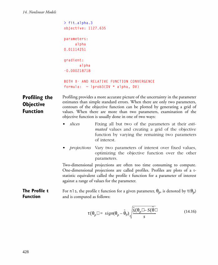
14. Nonlinear Models
> fit.alpha.3
objective: 1127.635
parameters:
alpha
0.01114251
gradient:
alpha
-0.000218718
BOTH X- AND RELATIVE FUNCTION CONVERGENCE
formula: ~ lprob3(DV * alpha, DV)
Profiling the
Objective
Function
Profiling provides a more accurate picture of the uncertainty in the parameterestimates than simple standard errors. When there are only two parameters,contours of the objective function can be plotted by generating a grid ofvalues. When there are more than two parameters, examination of theobjective function is usually done in one of two ways:
• slices Fixing all but two of the parameters at their esti-mated values and creating a grid of the objectivefunction by varying the remaining two parametersof interest.
• projections Vary two parameters of interest over fixed values,optimizing the objective function over the otherparameters.
Two-dimensional projections are often too time consuming to compute.One-dimensional projections are called profiles. Profiles are plots of a t-statistic equivalent called the profile t function for a parameter of interestagainst a range of values for the parameter.
The Profile t
Function
For nls, the profile t function for a given parameter, θp, is denoted by τ(θp)and is computed as follows:
(14.16)τ θp( ) sign θp θp–( )S θp( ) S θ( )–
s-------------------------------=
428

Inference for Nonlinear Models
where: is the model estimate of θp , is the sum of squares based
on optimizing all parameters except θp, which is fixed, and is the sum of
squares based on optimizing all parameters.
The profile t function is directly related to confidence intervals for thecorresponding parameter. τ(θp) can be shown to be equivalent to the
studentized parameter
for which a 1�α confidence interval can be constructed as follows:
The profile
Function in
S-PLUS
The profile function produces profiles for "nls" and "ms" objects. Profilesshow confidence intervals for parameters as well as the nonlinearity of theobjective function. If the model were linear the profile would be a straightline through the origin with a slope of one. You can produce the profile plotsfor the Puromycin fit Purboth as follows:
> Purboth.prof <- profile(Purboth)
> plot(Purboth.prof)
The "profile" object returned by profile has a component for eachparameter containing the evaluations of the profile t function plus someadditional attributes. The component for the Vm parameter is:
> Purboth.prof$Vm
tau par.vals.Vm par.vals.delV par.vals.K
1 -3.9021051 144.6497 54.60190 0.04501306
2 -3.1186052 148.8994 52.07216 0.04725929
3 -2.3346358 153.2273 49.54358 0.04967189
4 -1.5501820 157.6376 47.01846 0.05226722
5 -0.7654516 162.1334 44.50315 0.05506789
6 0.0000000 166.6040 42.02591 0.05797157
7 0.7548910 171.0998 39.57446 0.06103225
8 1.5094670 175.6845 37.12565 0.06431820
9 2.2635410 180.3616 34.67194 0.06783693
(14.17)
. (14.18)
θp˜ S θp( )
S θ( )
δ θp( )θp θp–
se θp( )-----------------=
t N P a2---;–
– δ θp( ) t N P a2---;–
≤ ≤
429

14. Nonlinear Models
10 3.0171065 185.1362 32.20981 0.07160305
11 3.7701349 190.0136 29.73812 0.07563630
12 4.5225948 194.9997 27.25599 0.07995897
Figure 14.2 shows profile plots for the three-parameter Puromycin fit. Eachplot shows the profile t function, (τ), when the parameter on the x-axisranges over the values shown, and the other parameters are optimized. Thesurface is quite linear with respect to these three parameters.
Computing
Confidence
Intervals
An example of a simple function to compute the confidence intervals fromthe output of profile follows:
> conf.int <- function(profile.obj, variable.name,
+ confidence.level = 0.95)
+ {if(is.na(match(variable.name, names(profile.obj))))
+ stop(paste("Variable", variable.name, "not in the model"))
+ resid.df <- attr(profile.obj, "summary")[["df"]][2]
+ tstat <- qt(1 - (1 - confidence.level)/2, resid.df)
+ prof <- profile.obj[[variable.name]]
+ approx(prof[, "tau"], prof[, "par.vals"][, variable.name],
+ c(-tstat, tstat))[[2]]
+ }
The tricky line in conf.int is the last one which calls approx.Purboth.prof$Vm is a data frame with two components (columns). Thefirst component is the vector of τ values which we pick off using prof[,"tau"]. The second component named par.vals contains a matrix with asmany columns as there are parameters in the model. This results in thestrange looking subscripting given by prof[, "par.vals"][,variable.name]. The first subscript removes the matrix from thepar.vals component, and the second subscript removes the appropriatecolumn. Three examples using conf.int and the profile objectPurboth.prof follow:
> conf.int(Purboth.prof, "delV", conf = .99)
[1] 24.20945 60.03857
> conf.int(Purboth.prof, "Vm", conf = .99)
[1] 150.4079 184.0479
> conf.int(Purboth.prof, "K", conf = .99)
[1] 0.04217613 0.07826822
The conf.int function can be improved by, for example, doing a cubicspline interpolation rather than the linear interpolation that approx does. Amarginal confidence interval computed from the profile t function is exact,
430

Inference for Nonlinear Models
disregarding any approximations due to interpolation, whereas the marginalconfidence intervals produced by using the coefficient and its standard errorfrom the summary of the fit is only a linear approximation.
Figure 14.2: The profile plots for the Puromycin fit.
Vmta
u
150 160 170 180 190
-4-2
02
4
delV
tau
20 30 40 50 60 70
-4-2
02
4
K
tau
0.04 0.06 0.08
-4-2
02
4
431

14. Nonlinear Models
432

DESIGNED EXPERIMENTS AND
ANALYSIS OF VARIANCE 15 Setting Up the Data Frame 435
The Model and Analysis of Variance 436
15.1 Experiments With One Factor 436
The One-Way Layout Model and Analysis of Variance 440
15.2 The Unreplicated Two-Way Layout 444
The Two-Way Model and ANOVA (One Observation per Cell) 448
15.3 The Two-Way Layout With Replicates 455
The Two-Way Model and ANOVA (With Replicates) 458
Method for Two-Factor Experiments With Replicates 461
Method for Unreplicated Two-Factor Experiments 463
Alternative Formal Methods 464
15.4 Many Factors at Two Levels: 2k Designs 465
Estimating All Effects in the 2k Model 468
Using Half-Normal Plots to Choose a Model 471
15.5 References 475
433

15. Designed Experiments and Analysis of Variance
434

DESIGNED EXPERIMENTS AND ANALYSIS
OF VARIANCE 15This chapter discusses how to analyze designed experiments. Typically, thedata have a numeric response and one or more categorical variables (factors)that are under the control of the experimenter. For example, an engineer maymeasure the yield of some process using each combination of four catalystsand three specific temperatures. This experiment has two factors, catalyst andtemperature, and the response is the yield.
Traditionally, the analysis of experiments has centered on the performance ofan Analysis of Variance (ANOVA). In more recent years graphics have playedan increasingly important role. There is a large literature on the design andanalysis of experiments�Box, Hunter, and Hunter (1978) is an example.
This chapter consists of sections which show you how to use Axum to analyzeexperimental data for each of the following situations:
� Experiments with one factor (section 15.1 )
� Experiments with two factors and a single replicate (section 15.2 )
� Experiments with two factors and two or more replicates(section 15.3)
� Experiments with many factors at two levels: 2k designs(section 15.4)
Each of these sections stands alone. You can read whichever section isappropriate to your problem, and get the analysis done without having toread the other sections. The examples used in sections 15.1�15.4 are fromBox, Hunter, and Hunter (1978). Thus, this chapter is a useful supplementin a course which covers the material of Chapters 6, 7, 9, 10, 11 of Box,Hunter, and Hunter.
Setting Up the
Data Frame
In analyzing experimental data using Axum, the first thing you do is set upan appropriate data frame for your experimental data. You may think of thedata frame as a matrix, with the columns containing values of the variables.Each row of the data frame contains an observed value of the response (orresponses), and the corresponding values of the experimental factors.
A First Look at
the Data
Use the functions plot.design, plot.factor and possiblyinteraction.plot to graphically explore your data.
435

15. Designed Experiments and Analysis of Variance
The Model and
Analysis of
Variance
It is important that you have a clear understanding of exactly what model isbeing considered when you carry out the analysis of variance. Use aov tocarry out the analysis of variance, and use summary to display the results.
In using aov, you use formulas to specify your model. The examples in thischapter introduce you to simple uses of formulas. You may supplement yourunderstanding of how to use formulas in Axum by reading chapter 2,Specifying Models in S-Plus, or chapter 2, Statistical Models, and chapter 5,Analysis of Variance; Designed Experiments, in Chambers and Hastie(1992).
Diagnostic Plots For each analysis, you should make the following minimal set of plots toconvince yourself that the model being entertained is adequate:
� Histogram of residuals (using hist)
� Normal qqplot of residuals (using qqnorm)
� Plot of residuals versus fit (using plot)
When you know the time order of the observations, you should also makeplots of the original data and the residuals in the time order in which the datawere collected.
The diagnostic plots may indicate inadequacies in the model from one ormore of the following sources: existence of interactions, existence of outliers,and existence of inhomogeneous error variance.
15.1 EXPERIMENTS WITH ONE FACTORThe simplest kind of experiments are those in which a single continuousresponse variable is measured a number of times for each of several levels ofsome experimental factor.
For example, consider the data in table 15.1 (from Box, Hunter, and Hunter(1978)), which consists of numerical values of �blood coagulation times� foreach of four diets. Coagulation time is the continuous response variable, anddiet is a qualitative variable, or factor, having four levels: A, B, C, and D. Thediets corresponding to the levels A, B, C, and D were determined by theexperimenter.
Your main interest is to see whether or not the factor �diet� has any effect onthe mean value of blood coagulation time. The experimental factor, �diet� inthis case, is often called the treatment.
Formal statistical testing for whether or not the factor level affects the mean iscarried out using the method of analysis of variance (ANOVA). This needs tobe complemented by exploratory graphics to provide confirmation that the
436

Experiments With One Factor
model assumptions are sufficiently correct to validate the formal ANOVAconclusion. Axum provides tools for you to do both the data exploration andformal ANOVA.
Setting Up the
Data Frame
In order to analyze the data, you need to get it into a form that Axum can usefor the analysis of variance. You do this by setting up a data frame. First createa numeric vector coag:
> coag <- scan()
1: 62 60 63 59
5: 63 67 71 64 65 66
11: 68 66 71 67 68 68
17: 56 62 60 61 63 64 63 59
25:
Next, create a factor called diet, that corresponds to coag:
> diet <- factor(rep(LETTERS[1:4],c(4,6,6,8)))
> diet
[1] A A A A B B B B B B C C C C C C D D D D D D D D
Now create a data frame with columns diet and coag:
> coag.df <- data.frame(diet,coag)
Table 15.1: Blood coagulation times for four diets.
Diet
A B C D
62 63 68 56
60 67 66 62
63 71 71 60
59 64 67 61
65 68 63
66 68 64
63
59
437

15. Designed Experiments and Analysis of Variance
The data frame object coag.df is a matrix-like object, so it looks like amatrix when you display it on your screen:
> coag.df
diet coag
1 A 62
2 A 60
3 A 63
.
.
.
23 D 63
24 D 59
A First Look at
the Data
For each level of the treatment factor, you make an initial graphicalexploration of the response data yij by using the functions plot.design and
plot.factor.
You can make plots of the treatment means and treatment medians for eachlevel of the experimental factor diet by using the function plot.designtwice, as follows:
> par(mfrow=c(1,2))
> plot.design(coag.df)
> plot.design(coag.df, fun= median)
> par(mfrow=c(1,1))
The results are shown in the two plots of figure 15.1. In the left hand plot,the tick marks on the vertical line are located at the treatment means for thediets A, B, C, and D, respectively. The mean values of coagulation time fordiets A and D happen to have the same value, 61, and so the labels A and Dare overlaid. The horizontal line, located at 64, indicates the overall mean ofall the data.
In the right hand plot of figure 15.1, medians rather than means areindicated. There is not much difference between the treatment means andthe treatment medians, so you should not be too concerned about adverseeffects due to outliers.
The function plot.factor produces a boxplot of the response data for eachlevel of the experimental factor:
438

Experiments With One Factor
Figure 15.1: Treatment means and medians.
Factors
mea
n of
coa
g
6264
6668
A
B
C
D
diet
Factors
med
ian
of c
oag
6264
6668
A
B
C
D
diet
439

15. Designed Experiments and Analysis of Variance
> plot.factor(coag.df)
The resulting plot is shown in figure 15.2. This plot indicates that theresponses for diets A and D are quite similar, while the median responses fordiets B and C are considerably larger relative to the variability reflected by theheights of the boxes. Thus, you suspect that diet has an effect on bloodcoagulation time.
If the exploratory graphical display of the response using plot.factorindicates that the interquartile distance of the boxplots depends upon themedian, then a transformation to make the error variance constant is calledfor. The transformation may be selected with a �spread versus level� plot. See,for example, section 15.3, or Hoaglin, Mosteller, and Tukey (1983).
The One-Way
Layout Model
and Analysis of
Variance
The classical model for experiments with a single factor is
Figure 15.2: Boxplots for each treatment.
60
65
70
co
ag
A B C D
diet
yij µi εi j+= j 1 … Ji, ,=
i 1 … I, ,=
440

Experiments With One Factor
where µi is the mean value of the response for the ith level of the
experimental factor. There are I levels of the experimental factor, and Ji
measurements are taken on the response variable for level i
of the experimental factor.
Using the treatment terminology, there are I treatments, and µi is called the
ith treatment mean. The above model is often called the one-way layoutmodel. For the blood coagulation experiment there are I=4 diets, and themeans µ1, µ2, µ3, and µ4 correspond to diets A, B, C, and D, respectively.
The numbers of observations are JA = 4, JB = JC = 6, and JD = 8.
You carry out the analysis of variance with the function aov:
> aov.coag <- aov(coag ~ diet, coag.df)
The first argument to aov above is the formula coag ~ diet. This formulais a symbolic representation of the one-way layout model equation; theformula excludes the error term εij. The second argument to aov is the data
frame you created, coag.df, which provides the data needed to carry out theANOVA. The names diet and coag, used in the formula coag ~ diet,need to match the names of the variables in the data frame coag.df.
To display the ANOVA table, use summary:
> summary(aov.coag)
Df Sum of Sq Mean Sq F Value Pr(F)
diet 3 228 76.0 13.5714 4.65847e-05
Residuals 20 112 5.6
The p-value is equal to .000047, which is highly significant.
Diagnostic Plots You obtain the fitted values and residuals using the fitted.values andresiduals functions on the result of aov. Thus, for example, you get thefitted values with the following:
> fitted.values(aov.coag)
1 2 3 4 5 6 7 8 9 10 11 12 13 14 15 16 17
61 61 61 61 66 66 66 66 66 66 68 68 68 68 68 68 61
18 19 20 21 22 23 24
61 61 61 61 61 61 61
The resid and fitted functions are shorter names for residuals andfitted.values, respectively.
You can check the residuals for distributional shape and outliers by usinghist and qqnorm, with the residuals component of aov.coag as argument:
yi1 yi2 … yiJi, , ,
441

15. Designed Experiments and Analysis of Variance
> hist(resid(aov.coag))
> qqnorm(resid(aov.coag))
Figure 15.3 shows the resulting histogram and figure 15.4 shows theresulting quantile-quantile plot.
Figure 15.3: Histogram of residuals.
Figure 15.4: Normal QQ-plot of residuals.
-6 -4 -2 0 2 4 6
02
46
8
resid(aov.coag)
•
•
•
•
•
•
•
•
•
• •
•
•
•
• •
•
•
•
•
•
•
•
•
Quantiles of Standard Normal
resi
d(a
ov.
coag)
-2 -1 0 1 2
-4-2
02
4
442

Experiments With One Factor
The shape of the histogram, and the linearity of the normal QQ-plot, bothindicate that the error distribution is quite Gaussian. (The flat sections in theQQ-plot are a consequence of tied values in the data.)
You can check for inhomogeneity of error variance and possible outliers byplotting the residuals versus the fit:
> plot(fitted(aov.coag), resid(aov.coag))
This plot reveals no unusual features, and is not shown.
Details An alternate form of the one-way layout model is the overall mean plus effectsform
yij = µ + αi +εij
where µ is the overall mean, and αi is the effect for level (or treatment) i. The
mean µi for level (or treatment) i in the first form of the model is related to µand αi by
µi = µ + αi
and the effects ai satisfy the constraint
.
The function aov fits the one-way model in the �overall mean plus effects�
form . See section 16.1 for more on this.
To obtain the effects, use model.tables as follows:
> model.tables(aov.coag)
Refitting model to allow projection
Tables of effects
diet
A B C D
-3 2 4 -3
rep 4 6 6 8
You can get the treatment means as follows:
> model.tables(aov.coag, type="means")
Refitting model to allow projection
Tables of means
Grand mean
64
α1 α2… αI+ + + 0=
yij µ αi r i j+ +=
443

15. Designed Experiments and Analysis of Variance
diet
A B C D
61 66 68 61
rep 4 6 6 8
15.2 THE UNREPLICATED TWO-WAY LAYOUTThe data in table 15.2 (used by Box, Hunter, and Hunter (1978)) werecollected to determine the effect of treatments A, B, C, and D on the yield ofpenicillin in a penicillin manufacturing process.
The values of the response variable �yield� are the numbers in the table, andthe columns of the table correspond to the levels A, B, C, and D of thetreatment factor. There was a second factor, namely the blend factor, since aseparate blend of the corn-steep liquor had to be made for each application ofthe treatments.
Your main interest is in determining whether the treatment factor affectsyield. The blend factor is of only secondary interest; it is a �blocking� variableintroduced to increase the sensitivity of the inference for treatments. Theorder of the treatments within blocks was chosen at random. Hence, this is arandomized blocks experiment.
The methods we use in this section applies equally well to two-factorexperiments in which both factors are experimentally controlled and of equalinterest.
Table 15.2: Effect of four treatments on penicillin yield.
Treatment
Block A B C D
Blend 1 89 88 97 94
Blend 2 84 77 92 79
Blend 3 81 87 87 85
Blend 4 87 92 89 84
Blend 5 79 81 80 88
444

The Unreplicated Two-Way Layout
Setting Up the
Data Frame
Table 15.2 is balanced�each entry or cell of the table (i.e., each row andcolumn combination) has the same number of observations (one observationper cell, in the present example)�so you can use fac.design to create thedata frame.
First, create a list fnames with two components named blend andtreatment, where blend contains the level names of the blend factor andtreatment contains the level names of the treatment factor:
> fnames <- list(blend=paste("Blend ", 1:5),
+ treatment=LETTERS[1:4])
Then use fac.design to create the design data frame pen.design
> pen.design <- fac.design(c(5,4), fnames)
The first argument, c(5,4), to fac.design specifies the design as havingtwo factors because its length is two. The 5 specifies five levels for the firstfactor, blend, and the 4 specifies four levels for the second factor, treatment.The second argument, fnames, specifies the factor names and the labels fortheir levels.
The design data frame pen.design that you just created contains the factorsblend and treatment as its first and second columns, respectively.
Now create yield to match pen.design:
> yield <- scan()
1: 89 84 81 87 79
6: 88 77 87 92 81
11: 97 92 87 89 80
16: 94 79 85 84 88
21:
You can now use data.frame to combine the design data framepen.design and the response yield into the data frame pen.df:
> pen.df <- data.frame(pen.design,yield)
Now look at pen.df:
> pen.df
blend treatment yield
1 Blend 1 A 89
2 Blend 2 A 84
3 Blend 3 A 81
4 Blend 4 A 87
5 Blend 5 A 79
6 Blend 1 B 88
.
.
445

15. Designed Experiments and Analysis of Variance
.
19 Blend 4 D 84
20 Blend 5 D 88
Alternatively, you could build the model data frame directly frompen.design as follows:
> pen.design[,"yield"] <- yield
When you plot the object pen.design, Axum uses the methodplot.design, because the object pen.design is of class design. Thus,you obtain the same results as if you called plot.design explicitly on theobject pen.df.
A First Look at
the Data
You can look at the (comparative) values of the sample means of the data foreach level of each factor using plot.design:
> plot.design(pen.df)
This function produces the plot shown in figure 15.5. For the blend factor,
each tick mark is located at the mean of the corresponding row of table 15.2.For the treatment factor, each tick mark is located at the mean of thecorresponding column of table 15.2. The horizontal line is located at thesample mean of all the data. Figure 15.5 suggests that the blend has a greatereffect on yield than does the treatment.
Figure 15.5: Sample means in penicillin yield experiment.
Factors
mea
n of
yie
ld
8284
8688
9092 Blend 1
Blend 2
Blend 3Blend 4
Blend 5
A
B
C
D
blend treatment
446

The Unreplicated Two-Way Layout
Since sample medians are insensitive to outliers, and sample means are not,you may want to make a plot similar to figure 15.5 using sample mediansinstead of sample means. You can do this with plot.design, using thesecond argument fun=median:
> plot.design(pen.df, fun=median)
In this case, the plot does not indicate great differences between samplemeans and sample medians.
Use plot.factor to get a more complete exploratory look at the data. Butfirst use par to get a one row by two column layout for two plots:
> par(mfrow=c(1,2))
> plot.factor(pen.df)
> par(mfrow=c(1,1))
This command produces the plot shown in figure 15.6 .
The boxplots for factors, produced by plot.factor, give additionalinformation about the data besides the location given by plot.design. Theboxplots indicate variability, skewness, and outliers in the response, for eachfixed level of each factor. For this particular data, the boxplots for both blendsand treatments indicate rather constant variability, relatively little overallskewness, and no evidence of outliers.
For two-factor experiments, you should use interaction.plot to checkfor possible interactions (i.e., non-additivity). The interaction.plotfunction does not accept a data frame as an argument. Instead, you must
Figure 15.6: Factor plot for penicillin yield experiment.
8085
9095
yiel
d
Blend 1 Blend 2 Blend 3 Blend 4 Blend 5
blend
8085
9095
yiel
d
A B C D
treatment
447

15. Designed Experiments and Analysis of Variance
supply appropriate factor names and the response name. To make these factorand response data objects available to interaction.plot, you must first�attach" the data frame pen.df:
> attach(pen.df)
> interaction.plot(treatment,blend,yield)
These commands produce the plot shown in figure 15.7.
The first argument to interaction.plot specifies which factor appearsalong the x-axis (in this case, treatment). The second argument specifieswhich factor is associated with each line plot, or �trace� (in this case, blend).The third argument is the response variable (in this case, yield).
Without replication it is often difficult to interpret an interaction plot sincerandom error tends to dominate. There is nothing striking in this plot.
The Two-Way
Model and
ANOVA (One
Observation
per Cell)
The additive model for experiments with two factors, A and B, and oneobservation per cell is:
Figure 15.7: Interaction plot of penicillin experiment.
treatment
mea
n
8085
9095
A B C D
blendBlend 1Blend 5Blend 3Blend 4Blend 2
yij µ αiA αi
B εi j+ + += i 1 … I, ,=
j 1 … J, ,=
448

The Unreplicated Two-Way Layout
where µ is the overall mean, is the effect of the ith level of factor A and
is the effect of the jth level of factor B.
For the penicillin data above, factor A is �blend� and factor B is �treatment.�Blend has I = 5 levels and treatment has J = 4 levels.
To estimate the additive model, use aov:
> aov.pen <- aov(yield ~ blend + treatment, pen.df)
The formula yield ~ blend + treatment specifies that a two factoradditive model is fit, with yield the response, and blend and treatmentthe factors.
Display the analysis of variance table with summary:
> summary(aov.pen)
Df Sum of Sq Mean Sq F Value Pr(F)
blend 4 264 66.0000 3.50442 0.040746
treatment 3 70 23.3333 1.23894 0.338658
Residuals 12 226 18.8333
The p-value for blend is moderately significant, while the p-value fortreatment is insignificant.
Diagnostic Plots Make a histogram of the residuals
> hist(resid(aov.pen))
The resulting histogram is shown in figure 15.8. Now make a normal QQ-plot of residuals:
> qqnorm(resid(aov.pen))
The resulting plot is shown in figure 15.9. The central four cells of thehistogram in figure 15.8 are consistent with a fairly normal distribution inthe middle. The linearity of the normal QQ-plot in figure 15.9, except nearthe ends, also suggests that the distribution is normal in the middle. Therelatively larger values of the outer two cells of the histogram, and theflattening of the normal QQ-plot near the ends, both suggest that the errordistribution is slightly more short-tailed than a normal distribution. This isnot a matter of great concern for the ANOVA F tests.
Make a plot of residuals versus the fit:
> plot(fitted(aov.pen), resid(aov.pen))
The resulting plot is shown in figure 15.10.
The plot of residuals versus fit gives some slight indication that smaller errorvariance is associated with larger values of the fit.
αiA
αjB
449

15. Designed Experiments and Analysis of Variance
Figure 15.8: Histogram of residuals for penicillin yield experiment.
Figure 15.9: Quantile-Quantile plot of residuals for penicillin yieldexperiment.
-6 -4 -2 0 2 4 6
01
23
45
resid(aov.pen)
•
•
•
•
•
•
•
•
•
•
•
•
•
•
•
•
•
•
•
•
Quantiles of Standard Normal
resi
d(ao
v.pe
n)
-2 -1 0 1 2
-4-2
02
46
450
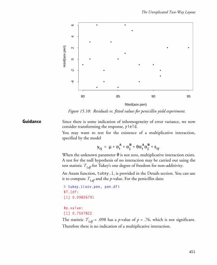
The Unreplicated Two-Way Layout
Guidance Since there is some indication of inhomogeneity of error variance, we nowconsider transforming the response, yield.
You may want to test for the existence of a multiplicative interaction,specified by the model
.
When the unknown parameter θ is not zero, multiplicative interaction exists.A test for the null hypothesis of no interaction may be carried out using thetest statistic T1df for Tukey�s one degree of freedom for non-additivity.
An Axum function, tukey.1, is provided in the Details section. You can useit to compute T1df and the p-value. For the penicillin data:
> tukey.1(aov.pen, pen.df)
$T.1df:
[1] 0.09826791
$p.value:
[1] 0.7597822
The statistic T1df = .098 has a p-value of p = .76, which is not significant.
Therefore there is no indication of a multiplicative interaction.
Figure 15.10: Residuals vs. fitted values for penicillin yield experiment.
•
•
•
•
•
•
•
•
•
•
•
•
•
•
•
•
•
•
•
•
fitted(aov.pen)
resi
d(ao
v.pe
n)
80 85 90 95
-4-2
02
46
yij µ αiA αj
B θαiAαj
B εi j+ + + +=
451

15. Designed Experiments and Analysis of Variance
Assuming that the response values are positive, you can find out whether ornot the data suggest a specific transformation to remove multiplicativeinteraction as follows: Plot the residuals rij for the additive fit versus the
comparison values
.
If this plot reveals a linear relationship with estimated slope , then you
should analyze the data again, using as new response values the power
transformation of the original response variables yij, with exponent
.
(If λ = 0, use log(yij).) See Hoaglin, Mosteller, and Tukey (1983) for details.
An Axum function called comp.plot, for computing the comparison values
cij, plotting rij versus cij, and computing , is provided in the Details section
below. Applying comp.plot to the penicillin data gives the following result:
> comp.plot(aov.pen, pen.df)
$theta.hat:
[1] 4.002165
$std.error:
[1] 9.980428
$R.squared:
R2
0.008854346
In this case the estimated slope is , which gives λ = -3. However, this is
not a very sensible exponent for a power transformation. The standard
deviation of is nearly 10 and the R2 is only .009, which indicates that θmay be zero. Thus we do not recommend using a power transformation.
cijαi
Aαj
B
µ--------------=
θ
yijλ
λ 1 θ–=
θ
θ 4=
θ
452

The Unreplicated Two-Way Layout
Details The test statistic T1df for Tukey�s one degree of freedom is given by:
where
SSres.1 = SSres - SSθ
Figure 15.11: Display from comp.plot.
•
•
••
•
•
•
•
•
•
•
•
•
•
•
•
•
•
•
•
cij
as.v
ecto
r(r.
ma
t)
-0.1 0.0 0.1 0.2
-4-2
02
46
T1df IJ I– J–( )SSθ
SSres.1-----------------=
SSθ
αiA
αjByij
j 1=
J
∑i 1=
I
∑ 2
αiA
( )2
i 1=
I
∑ αjB
( )2
j 1=
J
∑-----------------------------------------------=
SSres r ij2
j 1=
J
∑i 1=
I
∑=
453

15. Designed Experiments and Analysis of Variance
with the , the additive model estimates of the and , and rij
the residuals from the additive model fit. The statistic T1df has an F1,IJ-I-J
distribution.
Here is a function tukey.1 to compute the Tukey one-degree of freedom fornon-additivity test. You can create your own version of this function bytyping tukey.1 <- and then the definition of the function.
> tukey.1
function(aov.obj, data)
{
vnames <- names(aov.obj$contrasts)
if(length(vnames) != 2)
stop("the model must be two-way")
vara <- data[, vnames[1]]
varb <- data[, vnames[2]]
na <- length(levels(vara))
nb <- length(levels(varb))
resp <- data[, as.character(attr(aov.obj$terms,
"variables")[attr(aov.obj$terms, "response" )])]
cfs <- coef(aov.obj)
alpha.A <- aov.obj$contrasts[[vnames[1]]] %*% cfs[
aov.obj$assign[[vnames[1]]]]
alpha.B <- aov.obj$contrasts[[vnames[2]]] %*% cfs[
aov.obj$assign[[vnames[2]]]]
r.mat <- matrix(0, nb, na)
r.mat[cbind(as.vector(unclass(varb)), as.vector(
unclass(vara)))] <- resp
SS.theta.num <- sum((alpha.B %*% t(alpha.A)) *
r.mat)^2
SS.theta.den <- sum(alpha.A^2) * sum(alpha.B^2)
SS.theta <- SS.theta.num/SS.theta.den
SS.res <- sum(resid(aov.obj)^2)
SS.res.1 <- SS.res - SS.theta
T.1df <- ((na * nb - na - nb) * SS.theta)/SS.res.1
p.value <- 1 - pf(T.1df, 1, na * nb - na - nb)
list(T.1df = T.1df, p.value = p.value)
}
αiA
αjB
αiA αj
B
454

The Two-Way Layout With Replicates
Here is a function comp.plot for computing a least-squares fit to the plot ofresiduals versus comparison values:
> comp.plot
function(aov.obj, data)
{
vnames <- names(aov.obj$contrasts)
if(length(vnames) != 2)
stop("the model must be two-way")
vara <- data[, vnames[1]]
varb <- data[, vnames[2]]
cfs <- coef(aov.obj)
alpha.A <- aov.obj$contrasts[[vnames[1]]] %*% cfs[
aov.obj$assign[[vnames[1]]]]
alpha.B <- aov.obj$contrasts[[vnames[2]]] %*% cfs[
aov.obj$assign[[vnames[2]]]]
cij <- alpha.B %*% t(alpha.A)
cij <- c(cij)/cfs[aov.obj$assign$"(Intercept)"]
na <- length(levels(vara))
nb <- length(levels(varb))
r.mat <- matrix(NA, nb, na)
r.mat[cbind(as.vector(unclass(varb)), as.vector(
unclass(vara)))] <- resid(aov.obj)
plot(cij, as.vector(r.mat))
ls.fit <- lsfit(as.vector(cij), as.vector(r.mat))
abline(ls.fit)
output <- ls.print(ls.fit, print.it = F)
list(theta.hat = output$coef.table[2, 1], std.error
= output$coef.table[2, 2], R.squared =
output$summary[2])
}
15.3 THE TWO-WAY LAYOUT WITH REPLICATESThe data in table 15.3 (used by Box, Hunter, and Hunter (1978)) displaysthe survival times, in units of 10 hours, of animals in a replicatedfactorial experiment. In this experiment, each animal was given one of threepoisons, labeled I, II, and III, and one of four treatments, labeled A, B, C,and D. Four animals were used for each combination of poison andtreatment, making four replicates.
3 4×
455

15. Designed Experiments and Analysis of Variance
Setting Up the
Data Frame
To set up the data frame, first make a list, fnames, with componentstreatment and poison, containing the level names of these two factors:
> fnames <- list(treatment=LETTERS[1:4],
+ poison=c("I","II","III"))
Use fac.design, with optional argument rep=4, to create the design dataframe poisons.design:
> poisons.design <- fac.design(c(4,3), fnames, rep=4)
Note that since treatments is the first factor in the fnames list, andtreatments has 4 levels, 4 is the first argument of c(4,3).
Table 15.3: A replicated factorial experiment.
treatment
poison A B C D
I 0.31 0.82 0.43 0.45
0.45 1.10 0.45 0.71
0.46 0.88 0.63 0.66
0.43 0.72 0.76 0.62
II 0.36 0.92 0.44 0.56
0.29 0.61 0.35 1.02
0.40 0.49 0.31 0.71
0.23 1.24 0.40 0.38
III 0.22 0.30 0.23 0.30
0.21 0.37 0.25 0.36
0.18 0.38 0.24 0.31
0.23 0.29 0.22 0.33
456

The Two-Way Layout With Replicates
You now need to create the vector surv.time to match poisons.design.Each replicate of the experiment consists of data in three rows of table 15.3.Rows 1, 5, and 9 make up the first replicate, and so on. The command to getwhat we want is:
> surv.time <- scan()
1: .31 .82 .43 .45
5: .36 .92 .44 .56
9: .22 .30 .23 .30
13: .45 1.10 .45 .71
17: .29 .61 .35 1.02
21: .21 .37 .25 .36
25: .46 .88 .63 .66
29: .40 .49 .31 .71
33: .18 .38 .24 .31
37: .43 .72 .76 .62
41: .23 1.24 .40 .38
45: .23 .29 .22 .33
49:
Finally, make the data frame poisons.df:
> poisons.df <- data.frame(poisons.design, surv.time)
A First Look at
the Data
Use plot.design, plot.factor, and interaction.plot to get a firstlook at the data through summary statistics.
Set par(mfrow=c(3,2)) and use the above three functions to get the threerow and two column layout of plots displayed in figure 15.12:
> par(mfrow=c(3,2))
To obtain the design plot of sample means shown in the upper left plot offigure 15.12, use plot.design as follows:
> plot.design(poisons.df)
To obtain the design plot of sample medians shown in the upper right handplot of figure 15.12, use plot.design again:
> plot.design(poisons.df, fun=median)
The two sets of boxplots shown in the middle row of figure 15.12 areobtained with:
> plot.factor(poisons.df)
457

15. Designed Experiments and Analysis of Variance
To obtain the bottom row of figure 15.12, use interaction.plot:
> attach(poisons.df)
> interaction.plot(treatment,poison,surv.time)
> interaction.plot(treatment,poison,surv.time,fun=median)
The main differences between the plots obtained with plot.design usingmeans and medians are:
� the difference between the horizontal lines which represents themean and median, respectively, for all the data,
� the difference between the tick marks for the poison factor at level II.
The boxplots resulting from the use of plot.factor indicate a cleartendency for variability to increase with the (median) level of response.
The plots made with interaction.plot show stronger treatment effectsfor the two poisons with large levels than for the lowest level poison�anindication of an interaction.
The Two-Way
Model and
ANOVA (With
Replicates)
When you have replicates, you can consider a model which includes an
interaction term :
You can now carry out an ANOVA for the above model using aov as follows:
> aov.poisons <- aov(surv.time ~ poison*treatment,
+ poisons.df)
The expression poison*treatment on the right-hand side of the formulaspecifies that aov fit the above model with interaction. This contrasts withthe formula surv.time ~ poison + treatment, which tells aov to fit an
additive model for which is assumed to be zero for all levels i, j.
You now display the ANOVA table with summary:
> summary(aov.poisons)
Df Sum of Sq Mean Sq F Value Pr(F)
poison 2 1.033013 0.5165063 23.22174 0.0000003
treatment 3 0.921206 0.3070688 13.80558 0.0000038
poison:treatment 6 0.250138 0.0416896 1.87433 0.1122506
Residuals 36 0.800725 0.0222424
αi jAB
yijk µ αiA αj
B αi jAB εi jk+ + + += i 1 … I, ,=
j 1 … J, ,=
k 1 … K, ,=
αi jAB
458

The Two-Way Layout With Replicates
The p-values for both poisons and treatment are highly significant, while thep-value for interaction is insignificant.
The colon in poison:treatment denotes an interaction, in this case thepoison-treatment interaction.
Figure 15.12: Initial plots of the data.
Factors
mea
n of
sur
v.tim
e
0.3
0.5
A
B
C
D
I
II
III
treatment poison
Factors
med
ian
of s
urv.
time
0.3
0.5
A
B
C
D
I
II
III
treatment poison
0.2
0.6
1.0
surv
.tim
e
A B C D
treatment
0.2
0.6
1.0
surv
.tim
e
I II III
poison
treatment
mea
n of
sur
v.tim
e
0.2
0.4
0.6
0.8
A B C D
poison
IIIIII
treatment
med
ian
of s
urv.
time
0.2
0.4
0.6
0.8
A B C D
poison
IIIIII
459

15. Designed Experiments and Analysis of Variance
Diagnostic Plots Make a histogram and a normal QQ-plot of residuals, arranging the plotsside by side in a single figure with par(mfrow=c(1,2)) before using histand qqnorm:
> par(mfrow=c(1,2))
> hist(resid(aov.poisons))
> qqnorm(resid(aov.poisons))
> par(mfrow=c(1,1))
The call par(mfrow=c(1,1)), resets the plot layout to a single plot perfigure.
The histogram in the left-hand plot of figure 15.13 reveals a markedasymmetry, which is reflected in the normal QQ-plot in the right-hand sideof figure 15.13. The latter shows a curved departure from linearity towardthe lower left part of the plot, and a break in linearity in the upper right partof the plot. Evidently, all is not well (see the discussion on transforming thedata in the Guidance section below).
Make a plot of residuals versus fit:
plot(fitted(aov.poisons), resid(aov.poisons))
The result, displayed in figure 15.14, clearly reveals a strong relationshipbetween the residuals and the fitted values. The variability of the residualsincreases with increasing fitted values. This is another indication thattransformation would be useful.
Figure 15.13: Histogram and normal QQ-plot of residuals.
-0.4 -0.2 0.0 0.2 0.4
05
10
15
20
resid(aov.poisons)
••
••
••
•
•
•• ••
•
•
•
•
•
•
•
•
• •• • ••
•• •
•
•
••
••• •
•
•
•
•
•
•
•
•• • •
Quantiles of Standard Normal
resi
d(a
ov.
po
iso
ns)
-2 -1 0 1 2
-0.2
0.0
0.2
0.4
460

The Two-Way Layout With Replicates
Guidance When the error variance for an experiment varies with the expected value ofthe observations, a variance stabilizing transformation will often reduce oreliminate such behavior.
We shall show two methods for determining an appropriate variancestabilizing transformation, one which requires replicates and one which doesnot.
Method for
Two-Factor
Experiments
With
Replicates
For two-factor experiments with replicates, you can gain insight into anappropriate variance stabilizing transformation by carrying out the following
informal procedure. First, calculate the within-cell standard deviations
and means :
> std.poison <- tapply(poisons.df$surv.time,
+ list(poisons.df$treatment,
+ poisons.df$poison),var)^.5
> std.poison <- as.vector(std.poison)
> means.poison <- tapply(poisons.df$surv.time,
+ list(poisons.df$treatment,
+ poisons.df$poison),mean)
> means.poison <- as.vector(means.poison)
Figure 15.14: Plot of residuals versus fit.
••
• •
•
••
•
••
• •
•
•
•
•
•
•
•
•
••• • •
•
• ••
•
•
•
•
•• •
•
•
•
•
•
•
•
•
•
•• •
fitted(aov.poisons)
resi
d(ao
v.po
ison
s)
0.2 0.4 0.6 0.8
-0.2
0.0
0.2
0.4
σi j
yij
461

15. Designed Experiments and Analysis of Variance
Then plot versus , and use the slope of the regression line
to estimate the variance stabilizing transform:
> plot(log(means.poison),log(std.poison))
> var.fit <- lsfit(log(means.poison),
+ log(std.poison))
> abline(var.fit)
> theta <- var.fit$coef[2]
> theta
X
1.97704
Now let , and choose λ to be that value among the set of values
which is closest to . If λ = 0, then make the
transformation . Otherwise, make the power transformation
. Now you should repeat the complete analysis described in the
previous subsections, using the response in place of yijk.
Since for the poisons experiment you get , you choose λ = -1. This
gives a reciprocal transformation , where yijk are the values you
used in the response with surv.time. You can think of the new response
as representing the rate of dying.
The model can be refit using the transformed response:
> summary(aov(1/surv.time ~ poison*treatment, poisons.df))
Df Sum of Sq Mean Sq F Value Pr(F)
poison 2 34.87712 17.43856 72.63475 0.0000000
treatment 3 20.41429 6.80476 28.34307 0.0000000
poison:treatment 6 1.57077 0.26180 1.09042 0.3867329
Residuals 36 8.64308 0.24009
With the transformation the p-values for the main effects have decreasedwhile the p-value for the interaction has increased�a more satisfactory fit.The diagnostic plots with the new response are much improved also.
log σi j( ) log yij( )
λ 1 θ–=
1 12---– 0
12--- 1, , , ,–
λ
yi j log yij=
yi jk yijkλ
=
yi jk
θ 2≈
yi jk yijk1–=
yi jk
462

The Two-Way Layout With Replicates
Method for
Unreplicated
Two-Factor
Experiments
An alternative simple method for estimating the variance stabilizingtransformation is based on the relationship between the log of the absoluteresiduals and the log of the fitted values. This method has the advantage thatit can be used for unreplicated designs. This method is also often preferred to
that of plotting log against even for cases with replication, because
and are not always adequately good estimates of the mean and
standard deviation for small values of K (K<8).
This method consists of plotting log of absolute residuals versus log of fitted
values, and computing the slope of the regression line. You then set
. Residuals with very small absolute values should usually be
omitted before applying this method. Here is some sample code.
> plot(log(abs(fitted(aov.poisons)[
+ abs(resid(aov.poisons))>exp(-10)])),
+ log(abs(resid(aov.poisons)[
+ abs(resid(aov.poisons))>exp(-10)])))
> logrij.fit <- lsfit(
+ log(abs(fitted(aov.poisons)[
+ abs(resid(aov.poisons))>exp(-10)])),
+ log(abs(resid(aov.poisons)[
+ abs(resid(aov.poisons))>exp(-10)])))
> abline(logrij.fit)
> theta <- logrij.fit$coef[2]
> theta
X
1.930791
You get .
Note that the two simple methods described above both lead to nearlyidentical choices of power transformation to stabilize variance.
Details You will find that a non-constant standard deviation for observations yi (yijk
for the two-factor experiment with replicates) is well-explained by a powerlaw relationship in many datasets. In particular, for some constant B andsome exponent θ, we have
σi j yij
yij σi j
θ
λ 1 θ–=
λ 1 θ 1–≈–=
σy Bηθ≈
463

15. Designed Experiments and Analysis of Variance
where σy is the standard deviation of the yi and η is the mean of the yi. If you
then use a power law transformation
for some fixed exponent λ, it can be shown that the standard deviation
for the transformed data , is given by
.
You can therefore make have a constant value, independent of the mean
η of the original data yi (and independent of the approximate mean ηλ of the
transformed data ), by choosing
.
Note that
Suppose you plot log versus log for a two factor experiment with
replicates and find that this plot results in a fairly good straight line fit with
slope , where is an estimate of σy and is an estimate of η. Then the
slope provides an estimate of θ, and so you set . Since a
fractional exponent is not very natural, one often chooses the closest value
in the �natural� set:
Alternative
Formal
Methods
There are two alternative formal approaches to stabilizing the variance. Oneapproach is to select the power transformation that minimizes the residualsquared error. This is equivalent to maximizing the log-likelihood function,and is sometimes referred to as a Box-Cox analysis (see for example, Weisberg(1985); Box (1988); Haaland (1989))
yi yiλ
=
σy
yi
σy K ληλ 1 θ–( )–=
σy
yi
λ 1 θ–=
log σy log K θlog η+≈
σi j yi j
θ σi j yi j
θ λ 1 θ–=
λ
λ
1– Reciprocal
12---– Reciprocal square root
0 Log
12--- Square root
1 No transformation
464

Many Factors at Two Levels: 2k Designs
The second approach seeks to stabilize the variance without the use of atransformation, by including the variance function directly in the model.This approach is called generalized least squares/variance function estimation(see for example, Carroll and Ruppert (1988); Davidian and Haaland(1990)).
Transformations are easy to use and may provide a simpler, moreparsimonious model (Box (1988)). On the other hand, modeling thevariance function directly allows the analysis to proceed on the original scaleand allows more direct insight into the nature of the variance function. Incases when the stability of the variance is critical, either of these methodshave better statistical properties than the simple informal graphical methodsdescribed above.
15.4 MANY FACTORS AT TWO LEVELS: 2K DESIGNSThe data in table 15.4 come from an industrial product developmentexperiment in which a response variable called conversion is measured (inpercent) for each possible combination of two levels of four factors:
K catalyst charge (10 or 15 pounds),
Te temperature ( ),
P pressure (50 or 80 pounds per square inch),
C concentration (10% or 12%).
The levels are labeled �-� and �+� in the table. All the factors in theexperiment are quantitative, so the �-� indicates the �low� level and the �+�indicates the �high� level for each factor. This data set was used by Box,Hunter, and Hunter (1978).
The design for this experiment is called a 24 design, because there are 24 = 16possible combinations of two levels for four factors.
Setting Up the
Data Frame
To set up the data frame first create a list of the four factor names with thecorresponding pairs of levels labels:
> fnames <- list(K=c("10","15"), Te=c("220","240"),
+ P=c("50","80"), C=c("10","12"))
Now use fac.design to create the 2k design data frame devel.design:
> devel.design <- fac.design(rep(2,4), fnames)
The first argument to fac.design is a vector of length four, which specifiesthat there are four factors. Each entry of the vector is a 2, which specifies thatthere are two levels for each factor.
220 or 240°C
465

15. Designed Experiments and Analysis of Variance
Since devel.design matches table 15.4, you can simply scan in thecoversion data:
> conversion <- scan()
1: 71 61 90 82 68 61 87 80
9: 61 50 89 83 59 51 85 78
17:
Table 15.4: Data from product development experiment.
Factor
observation number
K Te P Cconversion
(%)run
order
1 – – – – 71 (8)
2 + – – – 61 (2)
3 – + – – 90 (10)
4 + + – – 82 (4)
5 – – + – 68 (15)
6 + – + – 61 (9)
7 – + + – 87 (1)
8 + + + – 80 (13)
9 – – – + 61 (16)
10 + – – + 50 (5)
11 – + – + 89 (11)
12 + + – + 83 (14)
13 – – + + 59 (3)
14 + – + + 51 (12)
15 – + + + 85 (6)
16 + + + + 78 (7)
466

Many Factors at Two Levels: 2k Designs
Finally, create the data frame devel.df:
> devel.df <- data.frame(devel.design, conversion)
> devel.df
K Te P C conversion
1 10 220 50 10 71
2 15 220 50 10 61
3 10 240 50 10 90
.
.
.
15 10 240 80 12 85
16 15 240 80 12 78
A First Look at
the Data
Use plot.design and plot.factor to make an initial graphicalexploration of the data. To see the design plot with sample means, use thefollowing command, which yields the plot shown in figure 15.15:
> plot.design(devel.df)
To see the design plot with sample medians, use:
> plot.design(devel.df, fun=median)
To see boxplots of the factors, use the following commands, which yield theplots shown in figure 15.16:
> par(mfrow=c(2,2))
> plot.factor(devel.df)
> par(mfrow=c(1,1))
Figure 15.15: Sample means for product development experiment.
Factors
mea
n of
con
vers
ion
6065
7075
8085
10
15
220
240
5080
10
12
K Te P C
467

15. Designed Experiments and Analysis of Variance
Estimating All
Effects in the
2k Model
You can use aov to estimate all effects (main effects and all interactions), andcarry out the analysis of variance. Let�s do so, and store the results inaov.devel:
> aov.devel <- aov(conversion ~ K*Te*P*C, devel.df)
The product form K*Te*P*C on the right-hand side of the formula tells
Axum to fit the above 24 design model with all main effects and allinteractions included. You can accomplish the same thing by using the powerfunction ^ to raise the expression K+Te+P+C to the 4th power:
> aov.devel <- aov(conversion ~ (K+Te+P+C)^4, devel.df)
This second method is useful when you want to specify only main effectsplus certain low-order interactions. For example, replacing 4 by 2 aboveresults in a model with all main effects and all second-order interactions.
You can obtain the estimated coefficients using the coef function on theaov output:
> coef(aov.devel)
(Intercept) K Te P C K:Te K:P Te:P K:C
72.25 -4 12 -1.125 -2.75 0.5 0.375 -0.625 -5.464379e-17
Figure 15.16: Factor plot for product development experiment.
5060
7080
90
conv
ersi
on
10 15
K
5060
7080
90
conv
ersi
on
220 240
Te
5060
7080
90
conv
ersi
on
50 80
P
5060
7080
90
conv
ersi
on
10 12
C
468

Many Factors at Two Levels: 2k Designs
Te:C P:C K:Te:P K:Te:C K:P:C Te:P:C K:Te:P:C
2.25 -0.125 -0.375 0.25 -0.125 -0.375 -0.125
Notice that colons are used to connect factor names to represent interactions,e.g., K:P:C is the three factor interaction between the factors K, P, and C.
For more on the relationship between coefficients, contrasts and effects, seesections 15.1 and 15.2.
You can get the analysis of variance table with the summary command :
> summary(aov.devel)
Df Sum of Sq Mean Sq
K 1 256.00 256.00
Te 1 2304.00 2304.00
P 1 20.25 20.25
C 1 121.00 121.00
K:Te 1 4.00 4.00
K:P 1 2.25 2.25
Te:P 1 6.25 6.25
K:C 1 0.00 0.00
Te:C 1 81.00 81.00
P:C 1 0.25 0.25
K:Te:P 1 2.25 2.25
K:Te:C 1 1.00 1.00
K:P:C 1 0.25 0.25
Te:P:C 1 2.25 2.25
K:Te:P:C 1 0.25 0.25
The ANOVA table does not provide any F statistics. This is because you haveestimated 16 parameters with 16 observations. There are no degrees offreedom left for estimating the error variance, and hence there is no errormean square to use as the denominator of the F statistics. However, theANOVA table can give you some idea of which effects are the maincontributors to the response variation.
469

15. Designed Experiments and Analysis of Variance
Estimating All
Effects in the 2k
Model With
Replicates
On some occasions, you may have replicates of a 2k design. In this case you
can estimate the error variance σ2, as well as all effects. For example, the data
in table 15.5 is from a replicated 23 pilot plant example used by Box, Hunter,and Hunter (1978). The three factors are temperature (Te), concentration (C)and catalyst (K ), and the response is yield.
To set up the data frame, first make the factor names list:
> fnames <- list(Te=c("Tl","Th"), C=c("Cl","Ch"),
+ K=c("Kl","Kh"))
Because T is a constant in Axum which stands for the logical value �true,� youcan not use T as a factor name for temperature. Instead, use Te, or some suchalternative abbreviation. Then make the design data frame, pilot.design,with M = 2 replicates, by using fac.design with the optional argumentrep=2:
> pilot.design <- fac.design(c(2,2,2), fnames, rep=2)
Now, create the response vector pilot.yield as a vector of length 16, withthe second replicate values following the first replicate values:
> pilot.yield <- scan()
1: 59 74 50 69 50 81 46 79
9: 61 70 58 67 54 85 44 81
17:
Table 15.5: Replicated pilot plant experiment.
Te C K rep 1 rep 2
– – – 59 61
+ – – 74 70
– + – 50 58
+ + – 69 67
– – + 50 54
+ – + 81 85
– + + 46 44
+ + + 79 81
470

Many Factors at Two Levels: 2k Designs
Finally, use data.frame:
> pilot.df <- data.frame(pilot.design, pilot.yield)
You can now carry out the ANOVA, and because the observations arereplicated, the ANOVA table has an error variance estimate, i.e., mean squarefor error, and F statistics:
> aov.pilot <- aov(pilot.yield ~ (Te + C + K)^3, pilot.df)
> summary(aov.pilot)
Df Sum of Sq Mean Sq F Value Pr(F)
Te 1 2116 2116 264.500 0.000000
C 1 100 100 12.500 0.007670
K 1 9 9 1.125 0.319813
Te:C 1 9 9 1.125 0.319813
Te:K 1 400 400 50.000 0.000105
C:K 1 0 0 0.000 1.000000
Te:C:K 1 1 1 0.125 0.732810
Residuals 8 64 8
Temperature is clearly highly significant, as is the temperature-catalystinteraction, and concentration is quite significant.
Estimating All
Small Order
Interactions
In cases where you are confident that high-order interactions are unlikely,you can fit a model which includes interactions only up to a fixed order,through the use of the power function ^ with an appropriate exponent. Forexample, in the product development experiment of table 15.4, you maywish to estimate only the main effects and all second-order interactions. Inthis case, use :
> aov.devel.2 <- aov(conversion ~ (K+Te+P+C)^2,devel.df)
Now you are using 16 observations to estimate 11 parameters: the mean, thefour main effects, and the six two-factor interactions. Since you only use 11degrees of freedom for the parameters, out of a total of 16, you still have 5degrees of freedom to estimate the error variance. So the command:
> summary(aov.devel.2)
will produce an ANOVA table with an error variance estimate and Fstatistics.
Using Half-
Normal Plots
to Choose a
Model
You are usually treading on thin ice if you assume that higher-orderinteractions are zero, unless you have extensive first-hand knowledge of the
process you are studying with a 2k design. When you are not sure whether ornot higher-order interactions are zero, you should use a half-normal quantile-
471

15. Designed Experiments and Analysis of Variance
quantile plot to judge which effects, including interactions of any order, aresignificant. Use the function qqnorm as follows to produce a half-normalplot on which you can identify points:
> qqnorm(aov.devel, label=6)
The resulting figure, with six points labeled, is shown in figure 15.17.
In general, there are 2k - 1 points in the half-normal plot, since there are 2k
effects and the estimate of the overall mean is not included in this plot. They-axis positions of the labeled points are the absolute values of the estimatedeffects. The messages you get from this plot are: You judge the effects fortemperature, catalyst, concentration, and temperature by concentration to beclearly non-zero. The effect for Pressure is also very likely non-zero. You canexamine the marginal effects better by creating a plot with a smaller y-range:
> qqnorm(aov.devel, label=6, ylim=c(0,20))
A full QQ-plot of the effects can give you somewhat more information. Toget this type of plot, use:
> qqnorm(aov.devel, full=T, label=6)
Having determined from the half-normal plot which effects are non-zero,now fit a model having terms for the main effects plus the interactionbetween temperature and concentration:
> aov.devel.small <- aov(conversion ~ K+P+Te*C, devel.df)
You can now get an ANOVA summary, including an error variance estimate:
> summary(aov.devel.small)
Df Sum of Sq Mean Sq F Value Pr(F)
Figure 15.17: Half-normal plot for product development experiment.
• • • • • • • • • • •• •
•
•
Half-normal Quantiles
Effe
cts
0.0 0.5 1.0 1.5 2.0
010
2030
40
Te
K C Te:C
P Te:P
472

Many Factors at Two Levels: 2k Designs
K 1 256.00 256.000 136.533 0.000000375
P 1 20.25 20.250 10.800 0.008200654
Te 1 2304.00 2304.000 1228.800 0.000000000
C 1 121.00 121.000 64.533 0.000011354
Te:C 1 81.00 81.000 43.200 0.000062906
Residuals 10 18.75 1.875
Diagnostic Plots Once you have tentatively identified a model for a 2k experiment, you shouldmake the usual graphical checks based on the residuals and fitted values. Inthe product development example, you should examine the following plots:
> hist(resid(aov.devel.small))
> qqnorm(resid(aov.devel.small))
> plot(fitted(aov.devel.small),resid(aov.devel.small))
The latter two plots are shown in figures 15.18 and 15.19.
You should also make plots using the time order of the runs:
> run.ord <- scan()
1: 8 2 10 4 15 9 1 13 16 5 11 14 3 12 6 7
17:
> plot(run.ord, resid(aov.devel.small))
> plot(run.ord, fitted(aov.devel.small))
Figure 15.18: Quantile-quantile plot of residuals, product developmentexample.
•
•
•••
•
•
••
•
•
•
• •
•
•
Quantiles of Standard Normal
resi
d(ao
v.de
vel.s
mal
l)
-2 -1 0 1 2
-2-1
01
2
473

15. Designed Experiments and Analysis of Variance
This gives a slight hint that the first runs were more variable than the latterruns.
Details The function aov returns, by default, coefficients corresponding to thefollowing �usual� ANOVA form for the ηi:
In this form of the 2k model, each im takes on just two values, 1 and 2. There
are 2k values of the k-tuple index i1i2...ik. The parameter µ is the overall
mean. The parameters , m = 1, �, k correspond to the main effects. The
parameters correspond to the two-factor interactions, the parameters
correspond to the three-factor interactions, and the remaining
coefficients are the higher-order interactions. The coefficients for the main
Figure 15.19: Fitted values vs. residuals, product development example.
•
•
•••
•
•
••
•
•
•
••
•
•
fitted(aov.devel.small)
resi
d(ao
v.de
vel.s
mal
l)
50 60 70 80 90
-2-1
01
2
ηi ηi1… i kµ αi1
1 αi2
2 … αi k
k+ + + += =
+ αi1i2
12 αi1i3
13 … αi k 1– i k
k 1 k,–+ + +
+ …
+ αi1i2… i k
123…k
αim
m
αimin
mn
αi l imin
lmn
474

References
effects satisfy the constraint . All higher-order
interactions satisfy the constraint that the sum over any individual subscript
index is zero, e.g. , etc.
Because of the constraints on the parameters in this form of the model, itsuffices to specify one of the two values for each effect. The function aov
returns estimates for the �high� levels, e.g., .
An estimated effect (in the sense usually used in 2k models) is equal to thedifference between the estimate at the high level minus the estimate at thelow level for the ANOVA model form given above:
and since
,
we have
.
15.5 REFERENCES
Box, G.E.P. and Hunter, W.G. and Hunter, J.S. (1978). Statistics forExperimenters: An Introduction to Design, Data Analysis. John Wiley, NewYork.
Box, G.E.P. (1988). Signal-to-noise ratios, performance criteria, andtransformations. Technometrics, 30:1�17.
Carroll, R.J. and Ruppert, D. (1988). Transformation and Weighting inRegression. Chapman and Hall, New York.
Chambers, J.M. and Hastie, T.J. (1992). Statistical Models in S. Wadsworthand Brooks Cole Advanced Books and Software, Pacific Grove, CA.
Davidian, M. and Haaland, P.D. (1990). Regression and calibration with non-constant error variance. Chemometrics and Intelligent Laboratory Systems;9:231�248.
Haaland, P. (1989). Experimental Design in Biotechnology. Marcel Dekker,New York.
Hoaglin, D.C. and Mosteller, F. and Tukey, J.W. (1983). UnderstandingRobust and Exploratory Data Analysis. John Wiley, New York.
α1i α2
i+ 0 i 1 … k, ,=,=
αi1112 αi12
12+ 0 α1i2i4
124 α2i2i4
124+ 0=,=
α2i α2
12,
α1 α21 α1
1–=
α11 α2
1+ 0=
α12α2
1=
475

15. Designed Experiments and Analysis of Variance
Weisberg, S. (1985). Applied Linear Regression, 2nd edition. John Wiley, NewYork.
476

FURTHER TOPICS IN ANALYSIS
OF VARIANCE 1616.1 Model Coefficients and Contrasts 479
16.2 Summarizing ANOVA Results 483
Splitting Treatment Sums of Squares Into Contrast Terms 484
Treatment Means and Standard Errors 485
Balanced Designs 485
2k Factorial Designs 489
Unbalanced Designs 489
Type III Sums of Squares and Adjusted Means 492
16.3 Multivariate Analysis of Variance 504
16.4 Split-Plot Designs 506
16.5 Repeated-Measures Designs 507
16.6 Rank Tests for One-Way and Two-Way Layouts 510
The Kruskal-Wallis Rank Sum Test 510
The Friedman Rank Sum Test 511
16.7 Variance Components Models 512
Estimating the Model 512
Estimation Methods 513
Random Slope Example 513
16.8 References 515
477

16. Further Topics in Analysis of Variance
478

FURTHER TOPICS IN ANALYSIS OF
VARIANCE 16The previous chapter, Designed Experiments and Analysis of Variance,describes the basic techniques for using Axum for analysis of variance. Thischapter extends the concepts to several related topics:
� Multivariate analysis of variance (MANOVA), discussed in thesection Multivariate Analysis of Variance, page 504.
� Split-plot designs (the section Split-Plot Designs, page 506).
� Repeated measures (the section Repeated-Measures Designs,page 507).
� Nonparametric tests for one-way and blocked two-way designs (thesection Rank Tests for One-Way and Two-Way Layouts, page 510)
� Variance components models (the section Variance ComponentsModels, page 512)
These topics are preceded by a discussion of model coefficients and contrasts(the section Model Coefficients and Contrasts, page 479); this information isimportant in interpreting the available ANOVA summaries, described in thesection Summarizing ANOVA Results, page 483.
16.1 MODEL COEFFICIENTS AND CONTRASTS
This section explains what the coefficients mean in ANOVA models, andhow to get more meaningful coefficients for particular cases.
Suppose we have 5 measurements of a response variable scores for each ofthree treatments, "A", "B", and "C", as shown below:
> scores
[1] 4 5 4 5 4 10 7 7 7 7 7 7 8 7 6
> scores.treat
[1] A A A A A B B B B B C C C C C
In solving the basic ANOVA problem, we are trying to solve the followingsimple system of equations:
µA µ αA+=
µB µ αB+=
µC µ αC+=
479

16. Further Topics in Analysis of Variance
The sample means , , and can be calculated directly from the data:
.
This leaves the following three equations in four unknowns:
.
Like all ANOVA models, this system is overparametrized, meaning there aremore coefficients than can be estimated. We can, however, replace the three
variables , , and with a pair of variables and that are
functionally independent linear combinations of the original variables, and
also independent of . Such a replacement can be done in more than one
way. For unordered factors such as scores.treat, the default choice inAxum is the set of Helmert contrasts :
.
These contrasts, in effect, contrast the ith level with the average of thepreceding levels.
More generally, if you have variables ai, i=1, �, k, you can reparametrize
with the k - 1 variables bj as follows:
. (16.1)
µA µB µC
µA 4 5 4 5 4+ + + +( ) 5⁄ 4.4= =
µB 10 7 7 7 7+ + + +( ) 5⁄ 7.6= =
µC 7 7 8 7 6+ + + +( ) 5⁄ 7.0= =
4.4 µ αA+=
7.6 µ αB+=
7.0 µ αC+=
αA αB αC β1 β2
µ
β1 αA– αB+=
β2 2αC αA αB+( )–=
βj jαj 1+ αii 1=
j
∑+=
480

Model Coefficients and Contrasts
The transpose of the matrix of coefficients for equation 16.1 is the followingk3 (k -1) contrast matrix:
You can recover the original treatment effects a from the reparametrizedvariables b by matrix multiplication as follows:
.
Returning to our simple example, we can rewrite our original variables in
terms of and as follows:
.
Axum now solves the following system of equations:
.
If we use aov as usual to create the aov object scores.aov, we can use the
coef function to look at the solved values , , and :
> scores.aov <- aov(scores ~ scores.treat)
> coef(scores.aov)
(Intercept) scores.treat1 scores.treat2
6.333333 1.6 0.3333333
In our example, the contrast matrix is as follows:
.
. (16.2)A
1– 1– 1– … 1–
1 1– 1– … 1–
0 2 1– … 1–
: : : : :
0 0 0 … k 1–
=
Ab a=
β1 β2
αA β1– β2–=
αB β1 β2–=
αC 2β2.=
4.4 µ β1– β2–=
7.6 µ β1 β2–+=
7.0 µ 2β2.+=
µ β1 β2
1– 1–
1 1–
0 2
481

16. Further Topics in Analysis of Variance
You can obtain the contrast matrix for any factor object using thecontrasts function. For unordered factors such as scores.treat,contrasts returns the Helmert contrast matrix of the appropriate size:
> contrasts(scores.treat)
[,1] [,2]
A -1 -1
B 1 -1
C 0 2
The contrast matrix, together with the treatment coefficients returned bycoef, provides an alternative to using model.tables to calculate effects:
> contrasts(scores.treat) %*% coef(scores.aov)[-1]
[,1]
A -1.9333333
B 1.2666667
C 0.6666667
For ordered factors, the Helmert contrasts are replaced, by default, withpolynomial contrasts that model the response as a polynomial through equallyspaced points. For example, suppose we define an ordered factorwater.temp as follows:
> water.temp <- ordered(c(65, 95, 120))
> water.temp
[1] 65 95 120
65 < 95 < 120
The contrast matrix for water.temp uses polynomial contrasts:
> contrasts(water.temp)
.L .Q
65 -0.7071068 0.4082483
95 0.0000000 -0.8164966
120 0.7071068 0.4082483
For the polynomial contrasts, represents the linear component of the
response, represents the quadratic component, and so on. When
examining ANOVA summaries, you can split a factor�s effects into contrastterms to examine each component�s contribution to the model. See thesection Splitting Treatment Sums of Squares Into Contrast Terms, page 484,for complete details.
β1
β2
482

Summarizing ANOVA Results
At times it is desirable to give particular contrasts to some of the coefficients.In our example, you might be interested in a contrast that has A equal to aweighted average of B and C. This might occur, for instance, if thetreatments were really doses. You can add a contrast attribute to the factorusing the assignment form of the contrasts function:
> contrasts(scores.treat) <- c(4,-1,-3)
> contrasts(scores.treat)
[,1] [,2]
A 4 0.2264554
B -1 -0.7925939
C -3 0.5661385
Note that a second contrast was automatically added.
Refitting the model, we now get different coefficients (but the fit remains thesame).
> scores.aov2 <- aov(scores ~ scores.treat)
> coef(scores.aov2)
(Intercept) scores.treat1 scores.treat2
6.333333 -0.4230769 -1.06434
More details on working with contrasts can be found in the sectionContrasts: The Coding of Factors, in chapter 2.
16.2 SUMMARIZING ANOVA RESULTS
Results from an analysis of variance are typically displayed in an analysis ofvariance table, which shows a decomposition of the variation in the response:the total sum of squares of the response is split into sums of squares for eachtreatment and interaction and a residual sum of squares. You can obtain theANOVA table, as we have throughout this chapter, by using summary on theresult of a call to aov, such as this overly simple model for the wafer data:
> attach(wafer)
> wafer.aov <- aov( pre.mean ~ visc.tem + devtime
+ + etchtime)
> summary(wafer.aov)
Df Sum of Sq Mean Sq F Value Pr(F)
visc.tem 2 1.343361 0.6716807 3.678485 0.0598073
devtime 2 0.280239 0.1401194 0.767369 0.4875574
etchtime 2 0.103323 0.0516617 0.282927 0.7588959
Residuals 11 2.008568 0.1825971
483

16. Further Topics in Analysis of Variance
Splitting
Treatment
Sums of
Squares Into
Contrast
Terms
Each treatment sum of squares in the ANOVA table can be further split intoterms corresponding to the treatment contrasts. By default, the Helmertcontrasts are used for unordered factors and polynomial contrasts for orderedfactors. For instance, with ordered factors you can assess whether theresponse is fairly linear in the factor by listing the polynomial contrastsseparately. In the dataset wafer, you can examine the linear and quadraticcontrasts of devtime and etchtime by using the split argument to thesummary function:
> summary(wafer.aov, split = list(etchtime =
+ list(L = 1, Q = 2),
+ devtime = list(L = 1, Q = 2)))
Df Sum of Sq Mean Sq F Value Pr(F)
visc.tem 2 1.343361 0.6716807 3.678485 0.0598073
devtime 2 0.280239 0.1401194 0.767369 0.4875574
devtime: L 1 0.220865 0.2208653 1.209577 0.2949025
devtime: Q 1 0.059373 0.0593734 0.325161 0.5799830
etchtime 2 0.103323 0.0516617 0.282927 0.7588959
etchtime: L 1 0.094519 0.0945188 0.517636 0.4868567
etchtime: Q 1 0.008805 0.0088047 0.048219 0.8302131
Residuals 11 2.008568 0.1825971
Each of the (indented) split terms sum to their overall sum of squares.
The split argument can evaluate only the effects of the contrasts used tospecify the ANOVA model: if you wish to test a specific contrast, you need toset it explicitly before fitting the model. Thus, if you want to test apolynomial contrast for an unordered factor, you must specify polynomialcontrasts for the factor before fitting the model. The same is true for othernon-default contrasts. For instance, the variable visc.tem in the waferdataset is a three-level factor constructed by combining two levels of viscosity(204 and 206) with two levels of temperature (90 and 105).
> levels(visc.tem)
[1] "204,90" "206,90" "204,105"
To assess viscosity, supposing temperature has no effect, we define a contrastthat takes the difference of the middle and the sum of the first and thirdlevels of visc.tem; the contrast matrix is automatically completed:
> contrasts(visc.tem) <- c(-1,2,-1)
> contrasts(visc.tem)
[,1] [,2]
204,90 -1 -7.071068e-01
206,90 2 -1.110223e-16
204,105 -1 7.071068e-01
484

Summarizing ANOVA Results
> wafer.aov <- aov( pre.mean ~ visc.tem + devtime
+ + etchtime)
In this fitted model, the first contrast for visc.aov reflects the effect ofviscosity:
> summary(wafer.aov, split = list(visc.tem = list(visc = 1)))
Df Sum of Sq Mean Sq F Value Pr(F)
visc.tem 2 1.343361 0.671681 3.678485 0.0598073
visc.tem: visc 1 1.326336 1.326336 7.263730 0.0208372
devtime 2 0.280239 0.140119 0.767369 0.4875574
etchtime 2 0.103323 0.051662 0.282927 0.7588959
Residuals 11 2.008568 0.182597
Treatment
Means and
Standard
Errors
Commonly the ANOVA model is written in the form �grand mean plustreatment effects,�
The treatment effects, ai, bj, (ab)ij reflect changes in the response due to
that combination of treatments. In this parameterization, the effects areconstrained, usually to sum to zero.
Unfortunately, the use of the term �effect� in ANOVA is not standardized: infactorial experiments an effect is the difference between treatment levels, inbalanced designs it is the difference from the grand mean, and in unbalanceddesigns there are (at least) two different standardizations that make sense.
The coefficients of an aov object returned by coef(aov.object) arecoefficients for the contrast variables derived by the aov function, rather thanthe grand-mean-plus-effects decomposition. The functions dummy.coef andmodel.tables translate the internal coefficients into the more naturaltreatment effects.
Balanced
Designs
In a balanced design, both computing and interpreting effects arestraightforward:
> gun.aov <- aov(Rounds ~ Method + Physique/Team, gun)
> coef(gun.aov)
(Intercept) Method Physique.L Physique.Q
19.33333 -4.255556 -1.154941 -0.06123724
PhysiqueSTeam1 PhysiqueATeam1 PhysiqueHTeam1
1.9375 0.45 -0.45
PhysiqueSTeam2 PhysiqueATeam2 PhysiqueHTeam2
-0.4875 0.008333333 -0.1083333
yijk µ αi βj αβ( )i j εi jk+ + + +=
485

16. Further Topics in Analysis of Variance
The dummy.coef function translates the coefficients into the more naturaleffects:
> dummy.coef(gun.aov)
$"(Intercept)":
(Intercept)
19.33333
$Method:
M1 M2
4.255556 -4.255556
$Physique:
[1] 0.7916667 0.0500000 -0.8416667
$"Team %in% Physique":
1T1 2T1 3T1 1T2 2T2
-1.45 -0.4583333 0.5583333 2.425 0.4416667
3T2 1T3 2T3 3T3
-0.3416667 -0.975 0.01666667 -0.2166667
For the default contrasts, these effects always sum to zero.
The same information is returned in a tabulated form by model.tablesNote that model.tables calls proj, hence it is helpful to use qr = T inthe call to aov.
> model.tables(gun.aov, se = T)
Refitting model to allow projection
Tables of effects
Method
M1 M2
4.256 -4.256
Physique
S A H
0.7917 0.05 -0.8417
486

Summarizing ANOVA Results
Team %in% Physique
Dim 1 : Physique
Dim 2 : Team
T1 T2 T3
S -1.450 2.425 -0.975
A -0.458 0.442 0.017
H 0.558 -0.342 -0.217
Standard errors of effects
Method Physique Team %in% Physique
0.3381 0.4141 0.7172
rep 18.0000 12.0000 4.0000
Using the first method, the gunners fired on average 4.26 more rounds thanthe overall mean. The standard errors for the effects are simply the residualstandard error scaled by the replication factor, rep, the number ofobservations at each level of the treatment. For instance, the standard errorfor the Method effect is:
The model.tables function also computes cell means for each of thetreatments. This provides a useful summary of the analysis that is more easilyrelated to the original data.
> model.tables(gun.aov, type = "means", se = T)
Tables of means
Grand mean
19.33
Method
M1 M2
23.59 15.08
Physique
S A H
20.13 19.38 18.49
se Method( ) se Residual( )
replication Method( )----------------------------------------------------- 1.434
18------------- 0.3381= = =
487

16. Further Topics in Analysis of Variance
Team %in% Physique
Dim 1 : Physique
Dim 2 : Team
T1 T2 T3
S 18.68 22.55 19.15
A 18.93 19.83 19.40
H 19.05 18.15 18.28
Standard errors for differences of means
Method Physique Team %in% Physique
0.4782 0.5856 1.014
rep 18.0000 12.0000 4.000
The first method had an average firing rate of 23.6 rounds. For the tables ofmeans, standard errors of differences between means are given, as these areusually of most interest to the experimenter. For instance the standard errorof differences for Team %in% Physique is
To gauge the statistical significance of the difference between the first andsecond small physique teams, we can compute the �least significant difference(LSD)� for the Team %in% Physique interaction. The validity of thestatistical significance is based on the assumption that the model is correctand the residuals are Gaussian. The plots of the residuals indicate these arenot unreasonable assumptions for this dataset�you can verify this bycreating a histogram and normal QQ-plot of the residuals as follows:
> hist(resid(gun.aov))
> qqnorm(resid(gun.aov))
The LSD at the 95% level is
.
We use the t-distribution with 26 degrees of freedom because the residualsum of squares has 26 degrees of freedom. In Axum, we type the following:
> qt(0.975, 26) * 1.014
[1] 2.084307
Since the means of the two teams differ by more than 2.08, the teams aredifferent at the 95% level of significance. From an interaction plot it is clearthat the results for teams of small physique are unusually high.
SED 22.0576
4----------------× 1.014= =
t 0.975 26,( ) SED Team %*% Physique( )×
488

Summarizing ANOVA Results
2k Factorial
Designs
In factorial experiments, where each experimental treatment has only twolevels, a treatment effect is, by convention, the difference between the highand low levels. Interaction effects are half the average difference betweenpaired levels of an interaction. These factorial effects are computed whentype = "feffects" is used in the model.tables function:
> catalyst.aov <- aov( Yield ~ ., catalyst, qr = T)
> model.tables(catalyst.aov, type = "feffects", se = T)
Table of factorial effects
Effects se
Temp 23.0 5.062
Conc -5.0 5.062
Cat 1.5 5.062
Unbalanced
Designs
When designs are unbalanced (there are unequal numbers of observations insome cells of the experiment), the effects associated with different treatmentlevels can be standardized in different ways. For instance, suppose we useonly the first 35 observations of the gun data set:
> gunsmall.aov <- aov(Rounds ~ Method
+ + Physique/Team, gun,
+ + subset=1:35, qr = T)
The dummy.coef function standardizes treatment effects to sum to zero:
> dummy.coef(gunsmall.aov)
$"(Intercept)":
(Intercept)
19.29177
$Method:
M1 M2
4.297115 -4.297115
$Physique:
[1] 0.83322650 0.09155983 -0.92478632
$"Team %in% Physique":
1T1 2T1 3T1 1T2 2T2
-1.45 -0.4583333 0.6830128 2.425 0.4416667
3T2 1T3 2T3 3T3
-0.2169872 -0.975 0.01666667 -0.466025
489

16. Further Topics in Analysis of Variance
The model.tables function computes effects that are standardized so the
weighted effects sum to zero: , where ni is the replication of
level i and ti the effect. The model.tables effects are identical to the values
of the projection vectors computed by proj(gunsmall.aov):
> model.tables(gunsmall.aov)
Tables of effects
Method
M1 M2
4.135 -4.378
rep 18.000 17.000
Physique
S A H
0.7923 0.05065 -0.9196
rep 12.0000 12.00000 11.0000
Team %in% Physique
Dim 1 : Physique
Dim 2 : Team
T1 T2 T3
S -1.450 2.425 -0.975
rep 4.000 4.000 4.000
A -0.458 0.442 0.017
rep 4.000 4.000 4.000
H 0.639 -0.261 -0.505
rep 4.000 4.000 3.000
With this standardization, treatment effects are orthogonal: consequently cellmeans can be computed by simply adding effects to the grand mean;standard errors are also more readily computed.
niτii 1=
T
∑ 0=
490

Summarizing ANOVA Results
> model.tables(gunsmall.aov, type="means", se=T)
Standard error information not returned as design
is unbalanced.
Standard errors can be obtained through se.contrast.
Tables of means
Grand mean
19.45
Method
M1 M2
23.59 15.08
rep 18.00 17.00
Physique
S A H
20.25 19.5 18.53
rep 12.00 12.0 11.00
Team %in% Physique
Dim 1 : Physique
Dim 2 : Team
T1 T2 T3
S 18.80 22.67 19.27
rep 4.00 4.00 4.00
A 19.05 19.95 19.52
rep 4.00 4.00 4.00
H 19.17 18.27 18.04
rep 4.00 4.00 3.00
Note that the (Intercept) value returned by dummy.coef is not the grandmean of the data, and the coefficients returned are not a decomposition ofthe cell means. This is a difference that occurs only with unbalanced designs:in balanced designs the functions dummy.coef and model.tables returnidentical values for the effects.
491

16. Further Topics in Analysis of Variance
In the unbalanced case, the standard errors for comparing two means dependon the replication factors, hence it could be very complex to tabulate allcombinations. Instead, they can be computed directly with se.contrast.For instance, to compare the first and third teams of heavy physique:
> se.contrast(gunsmall.aov, contrast = list(
+ Physique=="S" Team == "T1",
+ Physique=="S" Team == "T3"),
+ data = gun[1:35,])
[1] 1.018648
By default, the standard error of the difference of the means specified bycontrast is computed. Other contrasts are specified by the argument coef.For instance, to compute the standard error of the contrast tested in thesection Splitting Treatment Sums of Squares Into Contrast Terms, page 484,for the variable visc.tem:
> attach(wafer)
> se.contrast(wafer.aov, contrast = list(
+ visc.tem ==levels(visc.tem)[1],
+ visc.tem == levels(visc.tem)[2],
+ visc.tem == levels(visc.tem)[3]),
+ coef = c(-1,2,-1), data = wafer)
Refitting model to allow projection
[1] 0.07793052
The value of the contrast can be computed frommodel.tables(wafer.aov). The effects for visc.tem are:
visc.tem
204,90 206,90 204,105
0.1543 -0.3839 0.2296
The contrast is -0.3839 - mean(c(0.1543, 0.2296)) = -0.5758.The standard error for testing whether the contrast is zero is 0.0779; clearlythe contrast is nonzero.
Type III Sums
of Squares and
Adjusted
Means
Researchers implementing an experimental design frequently loseexperimental units and find themselves with unbalanced, but complete, data.The data is unbalanced in that the number of replications is not constant foreach treatment combination; the data is complete in that at least oneexperimental unit exists for each treatment combination. In this type ofcircumstance, an experimenter may find the hypotheses tested by Type IIIsum of squares are of more interest than those tested by Type I (sequential)sum of squares, and the adjusted means of more interest than unadjustedmeans. New options to the lm and aov object methods, anova.lm,
µ µijk i j k jkb f s fs= + + + + ( ) ,
492

Summarizing ANOVA Results
summary.aov, and model.tables.aov will give the Type III sum ofsquares and the adjusted (marginal) means. For anova and summary, thenew argument ssType can be 1 or 3, with ssType=1 as the default;model.tables has the new option �adj.means�, for the existingargument type. An example is given to demonstrate the new capabilities ofthese in an analysis of a designed experiment.
The fat-surfactant example is taken from Milliken and Johnson (1984, p.166), where they analyze an unbalanced randomized block factorial design.Here, the specific volume of bread loaves baked from dough mixed from eachof nine Fat and Surfactant treatment combinations is measured. Theexperimenters blocked on four flour types. Ten loaves had to be removedfrom the experiment, but at least one loaf existed for each Fat ✕ Surfactantcombination and all marginal means are estimable so the Type III hypothesesare testable.
The over-parameterized model is:
for i=1,..,4, j=1,2,3, and k=1,2,3. Because the data are unbalanced the TypeIII sum of squares for Flour, Fat and Surfactant test a more useful hypothesisthan the Type I. Specifically, the Type III hypotheses are that the marginalmeans are equal:
µ µijk i j k jkb f s fs= + + + + ( ) ,
H
H
H ,
Flour
Fat
Surfactant
:
:
:
.. .. .. ..
. . . . . .
.. .. ..
µ µ µ µµ µ µ
µ µ µ
1 2 3 4
1 2 3
1 2 3
= = == =
= =
493

16. Further Topics in Analysis of Variance
where
The hypotheses tested by the Type I sum of squares are not easily interpretedsince they are dependent on the order each term is specified the formula andinvolve the cell replications (which can be viewed as random variables whenthere are random drop-outs). Moreover, the hypothesis tested by the blockingterm, Flour, involves parameters of the Fat, Flour and Fat ✕ Flour terms.
ANOVA Tables The ANOVA tables for both Type I and Type III sum of squares are givenbelow for comparison. Using the Type III sum of squares we see that theblock effect, Flour, is significant as is Fat, but Surfactant is not at, say, a testsize of a = 0.05. However, in the presence of a significant interaction, the testof the marginal means probably has little meaning for Fat and Surfactant.
> Baking.aov<-aov(Specific.Vol ~ Flour + Fat * Surfactant,+ data = Baking, contrasts=list(Flour=contr.sum(4),+ Fat=contr.sum(3),Surfactant=contr.sum(3)) )
> anova(Baking.aov)
Analysis of Variance Table
Response: Specific.Vol
Terms added sequentially (first to last) Df Sum of Sq Mean Sq F Value Pr(F) Flour 3 6.39310 2.131033 12.88269 0.0002587 Fat 2 10.33042 5.165208 31.22514 0.0000069 Surfactant 2 0.15725 0.078625 0.47531 0.6313678Fat:Surfactant 4 5.63876 1.409691 8.52198 0.0010569 Residuals 14 2.31586 0.165418
µµ
µµ
µµ
i
ikjj k
j
ijki k
k
ijkij
..,
. .,
..
=⋅
=⋅
=⋅
∑
∑
∑
3 3
4 3
4 3 .
494

Summarizing ANOVA Results
> anova(Baking.aov,ssType=3)
Analysis of Variance Table
Response: Specific.Vol
Type III Sum of Squares Df Sum.of.Sq Mean.Sq F.Value Pr.F. Flour 3 8.69081 2.896937 17.51280 0.00005181 Fat 2 10.11785 5.058925 30.58263 0.00000778 Surfactant 2 0.99721 0.498605 3.01421 0.08153989Fat:Surfactant 4 5.63876 1.409691 8.52198 0.00105692 Residuals 14 2.31586 0.165418
Adjusted Means The adjusted (marginal) means given below estimate the means given in theType III hypotheses for Flour, Fat and Surfactant. The means for Flour ✕
Surfactant for the over-parameterized model are
Interestingly, these means are still estimable even though not all Flour ✕
Surfactant ✕ Flour combinations were observed.
> model.tables(Baking.aov,type="adj.means")
Tables of adjusted meansGrand mean
6.633281se 0.084599 N 26.000000
Flour 1 2 3 4 7.3020 5.7073 6.9815 6.5423 se 0.1995 0.1467 0.1621 0.1785rep 5.0000 8.0000 7.0000 6.0000
Fat 1 2 3 5.8502 6.5771 7.4725 se 0.1365 0.1477 0.1565rep 9.0000 9.0000 8.0000
µµ
⋅ =∑
jk
ijki
4
495

16. Further Topics in Analysis of Variance
Surfactant 1 2 3 6.3960 6.5999 6.9039 se 0.1502 0.1432 0.1473rep 8.0000 9.0000 9.0000
Fat:SurfactantDim 1 : FatDim 2 : Surfactant 1 2 3 1 5.5364 5.8913 6.1229 se 0.2404 0.2392 0.2414rep 3.0000 3.0000 3.0000 2 7.0229 6.7085 6.0000 se 0.2414 0.3006 0.2034rep 3.0000 2.0000 4.0000 3 6.6286 7.2000 8.5889 se 0.3007 0.2034 0.3001rep 2.0000 4.0000 2.0000
Multiple
Comparisons
The F-statistic for the Fat ✕ Surfactant interaction in the Type III ANOVAtable is significant so the tests for the marginal means for Fat and Surfactanthave little meaning. We can, however, use multicomp to find all pairwisecomparisons of the mean Fat levels for each level of Surfactant, and those forSurfactant for each level of Fat.
> multicomp(Baking.aov,focus="Fat",+ adjust=list(Surfactant=seq(3)))
95 % simultaneous confidence intervals for specifiedlinear combinations, by the Sidak method
critical point: 3.2117response variable: Flour
intervals excluding 0 are flagged by '****'
Estimate Std.Error Lower Bound Upper Bound1.adj1-2.adj1 -1.490 0.344 -2.590 -0.381 ****1.adj1-3.adj1 -1.090 0.377 -2.300 0.120 2.adj1-3.adj1 0.394 0.394 -0.872 1.660 1.adj2-2.adj2 -0.817 0.390 -2.070 0.434 1.adj2-3.adj2 -1.310 0.314 -2.320 -0.300 ****2.adj2-3.adj2 -0.492 0.363 -1.660 0.674 1.adj3-2.adj3 0.123 0.316 -0.891 1.140 1.adj3-3.adj3 -2.470 0.378 -3.680 -1.250 ****2.adj3-3.adj3 -2.590 0.363 -3.750 -1.420 ****
496

Summarizing ANOVA Results
> multicomp(Baking.aov,focus="Surfactant",+ adjust=list(Fat=seq(3)))
95 % simultaneous confidence intervals for specifiedlinear combinations, by the Sidak method
critical point: 3.2117response variable: Flour
intervals excluding 0 are flagged by '****'
Estimate Std.Error Lower Bound Upper Bound1.adj1-2.adj1 -0.355 0.341 -1.45000 0.740 1.adj1-3.adj1 -0.587 0.344 -1.69000 0.519 2.adj1-3.adj1 -0.232 0.342 -1.33000 0.868 1.adj2-2.adj2 0.314 0.377 -0.89700 1.530 1.adj2-3.adj2 1.020 0.316 0.00922 2.040 ****2.adj2-3.adj2 0.708 0.363 -0.45700 1.870 1.adj3-2.adj3 -0.571 0.363 -1.74000 0.594 1.adj3-3.adj3 -1.960 0.427 -3.33000 -0.590 ****2.adj3-3.adj3 -1.390 0.363 -2.55000 -0.225 ****
The levels for Fat and Surfactant factors are both labeled 1, 2, and 3 so therow labels in the multicomp tables require explanation. For the first table,the label 1.adj1-2.adj1 refers to the difference between levels 1 and 2 ofFat (the focus variable) at level 1of Surfactant (the adjust variable),whereas for the second table it is the difference between levels 1 and 2 ofSurfactant at level 1 of Fat. The reader can verify that the table of differencesreported by multicomp are the differences in the adjusted means forFat:Surfactant reported by model.tables. Significant differences areflagged with �****�. As a result of the of Surfactant and Fat interaction, theF test for the equivalence of the Surfactant marginal means is not significant,but there exists significant differences between the mean of Surfactant levels1-3 at a Fat level of 2 and between the means Surfactant levels 1-3 and 2-3at a Fat level of 3.
Estimable
Functions
The Type I and Type III estimable functions for the over-parameterizedmodel show the linear combinations of the over-parameterized modelparameters tested by each sum of squares. The Type I estimable functions canbe obtained by performing row reductions on the cross products of the
model matrix, XtX , that reduce it to upper triangular with each nonzero rowdivided by its diagonal (SAS Technical Report R-101, 1978).
497

16. Further Topics in Analysis of Variance
> round(L,4)
L2 L3 L4 L6 L7 L9 L10 L12 L13 L15 L16
(Intercept) 0.0000 0.0000 0.0000 0.0000 0.0000 0.0000 0.0000 0 0 0 0
Flour.1 1.0000 0.0000 0.0000 0.0000 0.0000 0.0000 0.0000 0 0 0 0
Flour.2 0.0000 1.0000 0.0000 0.0000 0.0000 0.0000 0.0000 0 0 0 0
Flour.3 0.0000 0.0000 1.0000 0.0000 0.0000 0.0000 0.0000 0 0 0 0
Flour.4 -1.0000 -1.0000 -1.0000 0.0000 0.0000 0.0000 0.0000 0 0 0 0
Fat.1 0.0667 -0.0833 0.0952 1.0000 0.0000 0.0000 0.0000 0 0 0 0
Fat.2 -0.3000 -0.1250 -0.2143 0.0000 1.0000 0.0000 0.0000 0 0 0 0
Fat.3 0.2333 0.2083 0.1190 -1.0000 -1.0000 0.0000 0.0000 0 0 0 0
Surfactant.1 0.2333 0.2083 0.1190 0.1152 0.1338 1.0000 0.0000 0 0 0 0
Surfactant.2 -0.1000 -0.2500 -0.2143 -0.1966 -0.3235 0.0000 1.0000 0 0 0 0
Surfactant.3 -0.1333 0.0417 0.0952 0.0814 0.1896 -1.0000 -1.0000 0 0 0 0
Fat.1:Surfactant.1 0.2000 0.1250 0.1429 0.3531 0.0359 0.3507 0.0037 1 0 0 0
Fat.2:Surfactant.1 -0.1667 -0.0417 -0.0238 -0.0060 0.3250 0.4242 0.0760 0 1 0 0
Fat.3:Surfactant.1 0.2000 0.1250 0.0000 -0.2319 -0.2271 0.2251 -0.0797 -1 -1 0 0
Fat.1:Surfactant.2 0.0333 -0.1667 -0.0238 0.3167 -0.0060 -0.0149 0.3499 0 0 1 0
Fat.2:Surfactant.2 -0.1667 -0.0417 -0.1667 0.0049 0.2034 0.0190 0.2971 0 0 0 1
Fat.3:Surfactant.2 0.0333 -0.0417 -0.0238 -0.5182 -0.5209 -0.0041 0.3530 0 0 -1 -1
Fat.1:Surfactant.3 -0.1667 -0.0417 -0.0238 0.3302 -0.0299 -0.3358 -0.3536 -1 0 -1 0
Fat.2:Surfactant.3 0.0333 -0.0417 -0.0238 0.0011 0.4716 -0.4432 -0.3731 0 -1 0 -1
Fat.3:Surfactant.3 0.0000 0.1250 0.1429 -0.2499 -0.2520 -0.2210 -0.2733 1 1 1
The columns labeled L2, L3, and L4 are for the Flour hypothesis; L6 and L7are for the Fat hypothesis; L9 and L10 are for the Surfactant hypothesis; andL12, L13, L15, and L16 are for the Fat ✕ Surfactant hypothesis. In contrast,the Type III estimable functions can be obtained from the generating set
(XtX)*(XtX), where (XtX)* is the g-2 inverse of the cross product matrix,(Kennedy and Gentle, 1980, p. 396) and perform the steps outlined in theSAS/STAT User�s Guide (1990, pp. 120-121) .
498

Summarizing ANOVA Results
> round(L3,4)
L2 L3 L4 L6 L7 L9 L10 L12 L13 L15 L16
(Intercept) 0 0 0 0.0000 0.0000 0.0000 0.0000 0 0 0 0
Flour.1 1 0 0 0.0000 0.0000 0.0000 0.0000 0 0 0 0
Flour.2 0 1 0 0.0000 0.0000 0.0000 0.0000 0 0 0 0
Flour.3 0 0 1 0.0000 0.0000 0.0000 0.0000 0 0 0 0
Flour.4 -1 -1 -1 0.0000 0.0000 0.0000 0.0000 0 0 0 0
Fat.1 0 0 0 1.0000 0.0000 0.0000 0.0000 0 0 0 0
Fat.2 0 0 0 0.0000 1.0000 0.0000 0.0000 0 0 0 0
Fat.3 0 0 0 -1.0000 -1.0000 0.0000 0.0000 0 0 0 0
Surfactant.1 0 0 0 0.0000 0.0000 1.0000 0.0000 0 0 0 0
Surfactant.2 0 0 0 0.0000 0.0000 0.0000 1.0000 0 0 0 0
Surfactant.3 0 0 0 0.0000 0.0000 -1.0000 -1.0000 0 0 0 0
Fat.1:Surfactant.1 0 0 0 0.3333 0.0000 0.3333 0.0000 1 0 0 0
Fat.2:Surfactant.1 0 0 0 0.0000 0.3333 0.3333 0.0000 0 1 0 0
Fat.3:Surfactant.1 0 0 0 -0.3333 -0.3333 0.3333 0.0000 -1 -1 0 0
Fat.1:Surfactant.2 0 0 0 0.3333 0.0000 0.0000 0.3333 0 0 1 0
Fat.2:Surfactant.2 0 0 0 0.0000 0.3333 0.0000 0.3333 0 0 0 1
Fat.3:Surfactant.2 0 0 0 -0.3333 -0.3333 0.0000 0.3333 0 0 -1 -1
Fat.1:Surfactant.3 0 0 0 0.3333 0.0000 -0.3333 -0.3333 -1 0 -1 0
Fat.2:Surfactant.3 0 0 0 0.0000 0.3333 -0.3333 -0.3333 0 -1 0 -1
Fat.3:Surfactant.3 0 0 0 -0.3333 -0.3333 -0.3333 -0.3333 1 1 1 1
Here we see one of the appealing properties of Type III sum of squares: thehypothesis tested by theType III sum of squares for Flour only involvesparameters of the Flour term, whereas the hypothesis tested by the Type Isum of squares for Flour involves the parameters of Fat, Surfactant and Fat ✕Surfactant.
The marginal means can also be obtained from multicomp usingcomparisons=�none�. Doing so, we obtain the estimable functions for themarginal means for the over-parameterized model. For example, theestimable functions for the Fat marginal means are:
> Fat.mcomp<-multicomp(Baking.aov,focus="Fat",comp="none")
499

16. Further Topics in Analysis of Variance
> round(Fat.mcomp$lmat,4)
1 2 3 (Intercept) 1.0000 1.0000 1.0000 Flour.1 0.2500 0.2500 0.2500 Flour.2 0.2500 0.2500 0.2500 Flour.3 0.2500 0.2500 0.2500 Flour.4 0.2500 0.2500 0.2500 Fat.1 1.0000 0.0000 0.0000 Fat.2 0.0000 1.0000 0.0000 Fat.3 0.0000 0.0000 1.0000 Surfactant.1 0.3333 0.3333 0.3333 Surfactant.2 0.3333 0.3333 0.3333 Surfactant.3 0.3333 0.3333 0.3333Fat.1:Surfactant.1 0.3333 0.0000 0.0000Fat.2:Surfactant.1 0.0000 0.3333 0.0000Fat.3:Surfactant.1 0.0000 0.0000 0.3333Fat.1:Surfactant.2 0.3333 0.0000 0.0000Fat.2:Surfactant.2 0.0000 0.3333 0.0000Fat.3:Surfactant.2 0.0000 0.0000 0.3333Fat.1:Surfactant.3 0.3333 0.0000 0.0000Fat.2:Surfactant.3 0.0000 0.3333 0.0000Fat.3:Surfactant.3 0.0000 0.0000 0.3333
The reader can verify that the Type III estimable functions for Fat are thedifferences between columns 1 and 3, and between columns 2 and 3.
Sigma
Constrained
Parameterization
The function lm reparameterizes the linear model in an attempt to make themodel matrix full column rank. We will next explore the computation of theadjusted means and the Type III sum of squares for Fat using the sigmaconstrained linear model. The sigma constraints were used in the aov fitabove (aov calls lm with singular.ok=T). This was done by specifyingcontr.sum in the contrasts argument. In this setting the adjusted meanscan be computed with the following estimable functions:
500

Summarizing ANOVA Results
> L
Fat.1 Fat.2 Fat.3 (Intercept) 1 1 1 Flour1 0 0 0 Flour2 0 0 0 Flour3 0 0 0 Fat1 1 0 -1 Fat2 0 1 -1 Surfactant1 0 0 0 Surfactant2 0 0 0Fat1Surfactant1 0 0 0Fat2Surfactant1 0 0 0Fat1Surfactant2 0 0 0Fat2Surfactant2 0 0 0
Some justification to these functions may be in order: The parameterizationchosen constrains the sum of the level estimates of each effect to zero. That is,
Therefore, any effect that we are summing over in the mean estimatevanishes. The intercept in the least squares fit estimates m and the twocoefficients for the Fat effect (labeled in L as Fat1 and Fat2) estimate f1 andf2, respectively and f3 = -f1 - f2.
We can check that each function is, in fact, estimable by ensuring that theyare in the row space of X, then compute the adjusted means.
> X<-model.matrix(Baking.aov)
> ls.fit<-lsfit(t(X)%*%X,L,intercept=F)
> apply(abs(ls.fit$residuals),2,max)<0.0001
Fat.1 Fat.2 Fat.3 T T T
> m<-t(L)%*%Baking.aov$coefficients
b f s fs fsi
i
j kk jkj jkkj∑ ∑ ∑ ∑∑= = = = =( ) ( ) 0 .
501

16. Further Topics in Analysis of Variance
> m
[,1]Fat.1 5.850197Fat.2 6.577131Fat.3 7.472514
Now use the summary method for the lm object to obtain (XtX)-1 and and compute the standard errors of the least squares means.
> Baking.sum<-summary.lm(Baking.aov)
> Baking.sum$sigma*sqrt(diag(t(L)%*%+ Baking.sum$cov.unscaled%*%L))
[1] 0.1364894 0.1477127 0.1564843
A set of Type III estimable functions for Fat can be obtained using thecontrasts generated by contr.helmert.
> contr.helmert(3)
[,1] [,2]1 -1 -12 1 -13 0 2
We will use this set of orthogonal contrasts to test and
which is equivalent to HFat.
> L.typeIII<-L%*%contr.helmert(3)
> L.typeIII
[,1] [,2] (Intercept) 0 0 Flour1 0 0 Flour2 0 0 Flour3 0 0 Fat1 -1 -3 Fat2 1 -3 Surfactant1 0 0 Surfactant2 0 0Fat1Surfactant1 0 0Fat2Surfactant1 0 0Fat1Surfactant2 0 0Fat2Surfactant2 0 0
�σ
µ µ⋅ ⋅ ⋅ ⋅=1 2
µ µ µ⋅ ⋅ ⋅ ⋅ ⋅ ⋅+ =1 2 32
502

Summarizing ANOVA Results
Finally, the Type III sum of squares is computed for Fat.
> h.m<-t(contr.helmert(3))%*%m
> t(h.m)%*%solve(t(L.typeIII)%*%Baking.sum$cov.unscaled%*%+ L.typeIII)%*%h.m
[,1][1,] 10.11785
Since we used the sigma-constrained model and the data is complete, we canalso use drop1 to obtain the Type III sum of squares.
> drop1(Baking.aov,~.)
Single term deletions
Model:Specific.Vol ~ Flour + Fat * Surfactant Df Sum of Sq RSS F Value Pr(F) <none> 2.31586 Flour 3 8.69081 11.00667 17.51280 0.00005181 Fat 2 10.11785 12.43371 30.58263 0.00000778 Surfactant 2 0.99721 3.31307 3.01421 0.08153989Fat:Surfactant 4 5.63876 7.95462 8.52198 0.00105692
For the sigma-constrained model, the hypotheses HFat and Hsurfactant can
also be expressed as
The row for Fat in the drop1 ANOVA table is the reduction in sum ofsquares due to Fat given all other terms are in the model. Thissimultaneously tests that the least squares coefficients bFat1 = f1 and bFat2 =
f2 are zero (and, hence f3 = -(f1 + f2) is zero) (Searle, 1987). The sameargument applies to Surfactant. It follows that the following Type IIIestimable functions for Fat can be used to test H*Fat (or equivalently HFat).
H
H = s = s = 0 .
*Fat
*Surfactant 2 3
:
:
f f
s
1 2
1
0= =
503

16. Further Topics in Analysis of Variance
> L.typeIII
[,1] [,2] (Intercept) 0 0 Flour1 0 0 Flour2 0 0 Flour3 0 0 Fat1 1 0 Fat2 0 1 Surfactant1 0 0 Surfactant2 0 0Fat1Surfactant1 0 0Fat2Surfactant1 0 0Fat1Surfactant2 0 0Fat2Surfactant2 0 0
> h.c<-t(L.typeIII)%*%Baking.aov$coef
> t(h.c)%*%solve(t(L.typeIII)%*%Baking.sum$cov.unscaled%*%+ L.typeIII)%*%h.c
[,1][1,] 10.11785
16.3 MULTIVARIATE ANALYSIS OF VARIANCE
Multivariate analysis of variance, known as MANOVA, is the extension ofanalysis of variance techniques to multiple responses. The responses for anobservation are considered as one multivariate observation, rather than as acollection of univariate responses.
If the responses are independent, then it is sensible to just perform univariateanalyses. However, if the responses are correlated, then MANOVA can bemore informative than the univariate analyses as well as less repetitive.
In Axum the manova function is used to estimate the model. The formulaneeds to have a matrix as the response:
> wafer.manova <- manova(cbind(pre.mean, post.mean) ~ .,
+ wafer[,c(1:9, 11)])
The manova function creates an object of class "manova". This class ofobject has methods specific to it for a few generic functions. The mostimportant function is the "manova" method for summary, which produces aMANOVA table:
504

Multivariate Analysis of Variance
> summary(wafer.manova)
Df Pillai Trace approx. F num df den df P-value
maskdim 1 0.9863 36.00761 2 1 0.11703
visc.tem 2 1.00879 1.01773 4 4 0.49341
spinsp 2 1.30002 1.85724 4 4 0.28173
baketime 2 0.80133 0.66851 4 4 0.64704
aperture 2 0.96765 0.93733 4 4 0.52425
exptime 2 1.63457 4.47305 4 4 0.08795
devtime 2 0.99023 0.98065 4 4 0.50733
etchtime 2 1.26094 1.70614 4 4 0.30874
Residuals 2
There are four common types of test in MANOVA. The example aboveshows the Pillai-Bartlett trace test, which is the default test in Axum. The lastfour columns show an approximate F test (since the distributions of the fourtest statistics are not implemented). The other available tests are Wilks�Lambda, Hotelling-Lawley trace, and Roy�s maximum eigenvalue. (By theway, a model with this few residual degrees of freedom is not likely toproduce informative tests.)
You can view the results of another test by using the test argument. Thefollowing command shows you Wilks� lambda test:
> summary(wafer.manova, test="wilk")
Below is an example of how to see the results of all four of the multivariatetests:
> wafer.manova2 <- manova(cbind(pre.mean, post.mean,
+ log(pre.dev), log(post.dev)) ~ maskdim + visc.tem
+ + spinsp, wafer)
> wafer.ms2 <- summary(wafer.manova2)
> for(i in c("p","w","h","r")) print(wafer.ms2, test=i)
You can also look at the univariate ANOVA tables for each response with acommand like:
> summary(wafer.manova, univariate=T)
Hand and Taylor (1987) provide a nice introduction to MANOVA. Manybooks on multivariate statistics contain a chapter on MANOVA. Examplesinclude Mardia, Kent and Bibby (1979), and Seber (1984).
505

16. Further Topics in Analysis of Variance
16.4 SPLIT-PLOT DESIGNS
A split-plot design contains more than one source of error. This can arisebecause factors are applied at different scales, as in the guayule examplebelow.
Split-plots are also encountered because of restrictions on the randomization.For example, an experiment involving oven temperature and baking time willprobably not randomize the oven temperature totally, but rather only changethe temperature after all of the runs for that temperature have been made.This type of design is often mistakenly analyzed as if there were norestrictions on the randomization (an indication of this can be p-values thatare close to 1). See Hicks (1973) and Daniel (1976).
Axum includes the guayule data frame which is also discussed in Chambersand Hastie (1992). This experiment was on eight varieties of guayule (arubber producing shrub) and four treatments on the seeds. Since a flat (ashallow box for starting seedlings) was not large enough to contain all 32combinations of variety and treatment, the design was to use only a singlevariety in each flat and to apply each treatment within each flat. Thus theflats each consist of four sub-plots. This is a split-plot design since flats arethe experimental unit for varieties, but the sub-plots are the experimentalunit for the treatments. The response is the number of plants that germinatedin each sub-plot.
To analyze a split-plot design like this, put the variable that corresponds tothe whole plot in an Error term in the formula of the aov call:
> gua.aov1 <- aov(plants ~ variety*treatment
+ + Error(flats), guayule)
As usual, you can get an ANOVA table with summary:
> summary(gua.aov1)
Error: flats
Df Sum of Sq Mean Sq F Value Pr(F)
variety 7 763.156 109.0223 1.232036 0.3420697
Residuals 16 1415.833 88.4896
Error: Within
Df Sum of Sq Mean Sq F Value Pr(F)
treatment 3 30774.28 10258.09 423.4386 0.00000e+00
variety:treatment 21 2620.14 124.77 5.1502 1.32674e-06
Residuals 48 1162.83 24.23
506

Repeated-Measures Designs
This shows varieties tested with the error from flats, while treatment and itsinteraction with variety are tested with the within-flat error (which issubstantially smaller).
The guayule data actually represent an experiment in which the flats weregrouped into replicates�making three sources of error, or a split-split-plotdesign. To model this we put more than one term inside the Error term:
> gau.aov2 <- aov(plants ~ variety*treatment
+ + Error(reps/flats), guayule)
> summary(gau.aov2)
Error: reps
Df Sum of Sq Mean Sq F Value Pr(F)
Residuals 2 38.58333 19.29167
Error: flats %in% reps
Df Sum of Sq Mean Sq F Value Pr(F)
variety 7 763.156 109.0223 1.108232 0.4099625
Residuals 14 1377.250 98.3750
Error: Within
Df Sum of Sq Mean Sq F Value Pr(F)
treatment 3 30774.28 10258.09 423.4386 0.00000e+00
variety:treatment 21 2620.14 124.77 5.1502 1.32674e-06
Residuals 48 1162.83 24.23
The Error term could also have been specified as Error(reps + flats).However, the specification Error(flats + reps) would not give thedesired result (the sequence within the Error term is significant); explicitlystating the nesting is preferred. Note that only one Error term is allowed.
16.5 REPEATED-MEASURES DESIGNS
Repeated-measures designs are those that contain a sequence of observations
on each subject�for example, a medical experiment in which each patient isgiven a drug, and observations are taken at zero, one, two and three weeksafter taking the drug. (The above description is a little too simplistic toencompass all repeated-measures designs, but it captures the spirit.)
Repeated-measures designs are similar to split-plot designs in that there ismore than one source of error (between subjects and within subjects), butthere is correlation in the within-subjects observations. In the example weexpect that the observations in week three will be more similar to week two
507

16. Further Topics in Analysis of Variance
observations than to week zero observations. Because of this, the split-plotanalysis (referred to as the univariate approach) is valid only under certainrestrictive conditions.
We will use the artificial dataset drug.mult, which has the following form:
> drug.mult
subject gender Y.1 Y.2 Y.3 Y.4
1 S1 F 75.9 74.3 80.0 78.9
2 S2 F 78.3 75.5 79.6 79.2
3 S3 F 80.3 78.2 80.4 76.2
4 S4 M 80.7 77.2 82.0 83.8
5 S5 M 80.3 78.6 81.4 81.5
6 S6 M 80.1 81.1 81.9 86.4
The dataset consists of the two factors subject and gender, and the matrixY which contains 4 columns. The first thing to do is stretch this out into aform suitable for the univariate analysis:
> drug.uni <- drug.mult[rep(1:6, rep(4,6)), 1:2]
> ymat <- data.matrix(drug.mult[,paste("Y.",1:4, sep="")])
> drug.uni <- cbind(drug.uni, time=ordered(rep(paste("Week",
+ 0:3,sep=""),6)), y=as.vector(t(ymat)))
The univariate analysis treats the data as a split-plot design:
> summary(aov(y ~ gender*time + Error(subject), drug.uni))
Error: subject
Df Sum of Sq Mean Sq F Value Pr(F)
gender 1 60.80167 60.80167 19.32256 0.01173
Residuals 4 12.58667 3.14667
Error: Within
Df Sum of Sq Mean Sq F Value Pr(F)
time 3 49.10833 16.36944 6.316184 0.0081378
gender:time 3 14.80167 4.93389 1.903751 0.1828514
Residuals 12 31.10000 2.59167
Tests in the �Within� stratum are valid only if the data satisfy the�circularity� property, in addition to the usual conditions. Circularity meansthat the variance of the difference of measures at different times is constant;for example, the variance of the difference between the measures at week 0and week 3 should be the same as the variance of the difference between week2 and week 3. We also need the assumption that actual contrasts are used; forexample, the contr.treatment function should not be used. Whencircularity does not hold, then the p-values for the tests will be too small.
508

Repeated-Measures Designs
One approach is to perform tests which are as conservative as possible.Conservative tests are formed by dividing the degrees of freedom in both thenumerator and denominator of the F test by the number of repeatedmeasures minus one. In our example there are four repeated measures oneach subject, so we divide by 3. The split-plot and the conservative tests are:
> 1 - pf(6.316184, 3, 12) # usual univariate test
[1] 0.008137789
> 1 - pf(6.316184, 1, 4) # conservative test
[1] 0.06583211
These two tests are telling fairly different tales, so the data analyst wouldprobably move on to one of two alternatives. A Huynh-Feldt adjustment ofthe degrees of freedom provides a middle ground between the tests above�see Winer, Brown and Michels (1991), for instance. The multivariateapproach, discussed below, substantially relaxes the assumptions.
The univariate test for �time� was really a test on three contrasts. In themultivariate setting we want to do the same thing, so we need to use contrastsin the response:
> drug.man <- manova(ymat %*% contr.poly(4) ~ gender,
+ drug.mult)
> summary(drug.man, intercept=T)
Df Pillai Trace approx. F num df den df P-value
(Intercept) 1 0.832005 3.301706 3 2 0.241092
gender 1 0.694097 1.512671 3 2 0.421731
Residuals 4
The line marked �(Intercept)� corresponds to �time� in the univariateapproach, and similarly the �gender� line here corresponds to �gender:time�.The p-value of .24 is larger than either of the univariate tests�the price ofthe multivariate analysis being more generally valid is that quite a lot ofpower is lost. Although the multivariate approach is preferred when the datado not conform to the required conditions, the univariate approach ispreferred when they do (the trick, of course, is knowing which is which).
Let�s look at the univariate summaries that this MANOVA produces:
> summary(drug.man, intercept=T, univar=T)
Response: .L
Df Sum of Sq Mean Sq F Value Pr(F)
(Intercept) 1 22.188 22.1880 4.327255 0.1059983
gender 1 6.912 6.9120 1.348025 0.3101900
Residuals 4 20.510 5.1275
509

16. Further Topics in Analysis of Variance
Response: .Q
Df Sum of Sq Mean Sq F Value Pr(F)
(Intercept) 1 5.415000 5.415000 5.30449 0.0826524
gender 1 4.001667 4.001667 3.92000 0.1188153
Residuals 4 4.083333 1.020833
Response: .C
Df Sum of Sq Mean Sq F Value Pr(F)
(Intercept) 1 21.50533 21.50533 13.22049 0.0220425
gender 1 3.88800 3.88800 2.39016 0.1969986
Residuals 4 6.50667 1.62667
If you add up the respective degrees of freedom and sums of squares, you willfind that the result is the same as the univariate �Within� stratum. For thisreason, the univariate test is sometimes referred to as the �average F test�.
The above discussion has focused on classical inference, which should not bedone before graphical exploration of the data.
Many books discuss repeated measures. Some examples are Hand and Taylor(1987), Milliken and Johnson (1984), Crowder and Hand (1990), Winer,Brown and Michels (1991).
16.6 RANK TESTS FOR ONE-WAY AND TWO-WAY LAYOUTS
This section briefly describes how to use two non-parametric rank tests forANOVA: the Kruskal-Wallis rank sum test for a one-way layout and theFriedman test for unreplicated two-way layout with (randomized) blocks.
Since these tests are based on ranks, they are robust with regard to thepresence of outliers in the data; that is, they are not affected very much byoutliers. This is not the case for the classical F tests.
You can find detailed discussions of the Kruskal-Wallis and Friedman rank-based tests in a number of books on nonparametric tests; for example,Lehmann (1975) and Hettmansperger (1984).
The Kruskal-
Wallis Rank
Sum Test
When you have a one-way layout, as in the section Experiments With OneFactor in the previous chapter, you can use the Kruskal-Wallis rank sum testkruskal.test to test the null hypothesis that all group means are equal.
We illustrate how to use kruskal.test for the blood coagulation data of15.1. First you set up your data as for a one-factor experiment (or one-waylayout). You create a vector object coag, arranged by factor level (ortreatment), and you create a factor object diet whose levels correspond tothe factor levels of vector object coag. Then use kruskal.test:
510

Rank Tests for One-Way and Two-Way Layouts
> kruskal.test(coag,diet)
Kruskal-Wallis rank sum test
data: coag and diet
Kruskal-Wallis chi-square = 17.0154, df = 3,
p-value = 7e-04
alternative hypothesis: two.sided
The p-value of p = .0007 is highly significant. This p-value is computedusing an asymptotic chi-squared approximation. See the help file for moredetails.
You may find it helpful to note that kruskal.test and friedman.testreturn the results of its computations, and associated information, in thesame style as the functions in chapter 3, Statistical Inference for One andTwo Sample Problems.
The Friedman
Rank Sum Test
When you have a two-way layout with one blocking variable and onetreatment variable, you can use the Friedman rank sum test friedman.testto test the null hypothesis that there is no treatment effect.
We illustrate how you use friedman.test for the penicillin yield datadescribed in 15.2 of the previous chapter. The general form of the usage is
friedman.test(y,groups,blocks)
where y is a numeric vector, groups contains the levels of the treatmentfactor and block contains the levels of the blocking factor. Thus you can do:
> attach(pen.df) # make treatment and blend available
> friedman.test(yield, treatment, blend)
Friedman rank sum test
data: yield and pen.design[, 2] and pen.design[, 1]
Friedman chi-square = 3.4898, df = 3, p-value = 0.3221
alternative hypothesis: two.sided
The p-value is p=.32, which is not significant. This p-value is computedusing an asymptotic chi-squared approximation. For further details onfriedman.test, see the help file.
511

16. Further Topics in Analysis of Variance
16.7 VARIANCE COMPONENTS MODELS
Variance components models are used when there is interest in the variabilityof one or more variables other than the residual error. For example,manufacturers often run experiments to see which parts of the manufacturingprocess contribute most to the variability of the final product. In thissituation variability is undesirable, and attention is focused on improvingthose parts of the process that are most variable. Animal breeding is anotherarea in which variance components models are routinely used. Some data,from surveys for example, that have traditionally been analyzed usingregression can more profitably be analyzed using variance componentmodels.
Estimating the
Model
To estimate a variance component model, you first need to use is.randomto state which factors in your data are random. A variable that is marked asbeing random will have a variance component in any models that contain it.Only variables that inherit from class "factor" can be declared random.Although is.random works on individual factors, it is often more practicalto use it on the columns of a data frame. You can see if variables are declaredrandom by using is.random on the data frame:
> is.random(pigment)
Batch Sample Test
F F F
Declare variables to be random by using the assignment form of is.random:
> is.random(pigment) <- c(T, T, T)
> is.random(pigment)
Batch Sample Test
T T T
Because we want all of the factors to be random, we could have simply donethe following:
> is.random(pigment) <- T
The value on the right is replicated to be the length of the number of factorsin the data frame.
Once you have declared your random variables, you are ready to estimate themodel using the varcomp function. This function takes a formula and otherarguments very much like lm or aov. Because the pigment data are from anested design, the call has the following form:
> pigment.vc <- varcomp(Moisture ~ Batch/Sample, pigment)
512

Variance Components Models
> pigment.vc
Variances:
Batch Sample %in% Batch Residuals
7.127976 28.53333 0.9166667
Call:
varcomp(formula = Moisture ~ Batch/Sample, data = pigment)
The result of varcomp is an object of class "varcomp". You can usesummary on "varcomp" objects to get more details about the fit, and youcan use plot to get QQ-plots for the normal distribution on the estimatedeffects for each random term in the model.
Estimation
Methods
The method argument to varcomp allows you to choose the type of variancecomponent estimator. Maximum likelihood and REML (restrictedmaximum likelihood) are two of the choices. REML is very similar tomaximum likelihood but takes the number of fixed effects into account (theusual unbiased estimate of variance in the one-sample model is a REMLestimate). See Harville (1977) for more details on these estimators.
The default method is a MINQUE (minimum norm quadratic unbiasedestimate); this class of estimator is locally best at a particular spot in theparameter space. The MINQUE option in Axum is locally best if all of thevariance components (except that for the residuals) are zero. The MINQUEestimate agrees with REML for balanced data. See Rao (1971) for details.This method was made the default because it is less computationally intensethan the other methods, however, it can do significantly worse for severelyunbalanced data (Swallow and Monahan (1984)).
You can get robust estimates by using "method=winsor". This methodcreates new data by moving outlying points or groups of points toward therest of the data. One of the standard estimators is then applied to thispossibly revised data. Burns (1992) gives details of the algorithm along withsimulation results. This method uses much larger amounts of memory thanthe other methods if there are a large number of random levels, such as in adeeply nested design.
Random Slope
Example
We now produce a more complicated example in which there are randomslopes and intercepts. The data consist of several pairs of observations on eachof several individuals in the study. An example might be that the y valuesrepresent the score on a test and the x values are the time at which the testwas taken.
513

16. Further Topics in Analysis of Variance
Let�s start by creating simulated data of this form. We create data for 30subjects and 10 observations per subject:
> subject <- factor(rep(1:30, rep(10,30)))
> set.seed(357) # makes these numbers reproducible
> trueslope <- rnorm(30, mean=1)
> trueint <- rnorm(30, sd=.5)
> times <- rchisq(300, 3)
> scores <- rep(trueint, rep(10,30)) + times *
+ rep(trueslope, rep(10,30)) + rnorm(300)
> test.df <- data.frame(subject, times, scores)
> is.random(test.df) <- T
> is.random(test.df) subject T
Even though we want to estimate random slopes and random intercepts, theonly variable that is declared random is subject. Our model for the data hastwo coefficients: the mean slope (averaged over subjects) and the meanintercept. It also has three variances: the variance for the slope, the variancefor the intercept, and the residual variance.
The following command estimates this model using Maximum Likelihood(the default MINQUE is not recommended for this type of model):
> test.vc <- varcomp(scores ~ times * subject,
+ data=test.df, method="ml")
This seems very simple. We can see how it works by looking at how theformula get expanded. The right side of the formula is expanded into fourterms:
scores ~ 1 + times + subject + times:subject
The intercept term in the formula, represented by 1, gives the meanintercept. The variable times is fixed and produces the mean slope. Thesubject variable is random and produces the variance component for therandom intercept. Since any interaction containing a random variable isconsidered random, the last term, times:subject, is also random; thisterm gives the variance component for the random slope. Finally, there isalways a residual variance.
Now we can look at the estimates:
> test.vc
Variances:
subject times:subject Residuals
0.3162704 1.161243 0.8801149
Message:
[1] "RELATIVE FUNCTION CONVERGENCE"
514

References
Call:
varcomp(formula = scores ~ times*subject, data=test.df,
method = "ml")
This shows the three variance components. The variance of the intercept,which has true value .25, is estimated as .32. Next, labeled times:subjectis the variance of the slope, and finally the residual variance. We can also viewthe estimates for the coefficients of the model, which have true values of 0and 1.
> coef(test.vc)
(Intercept) times
0.1447211 1.02713
16.8 REFERENCES
Burns, P. J. (1992). Winsorized REML estimates of variance components.Submitted.
Chambers, J.M. and Hastie, T.J. (1992). Statistical Models in S. Wadsworthand Brooks Cole Advanced Books and Software, Pacific Grove, CA.
Crowder, M. J. and Hand, D. J. (1990). Analysis of Repeated Measures.Chapman and Hall, London.
Daniel, C. (1976). Applications of Statistics to Industrial Experimentation.Wiley, New York.
Hand, D. J. and Taylor, C. C. (1987). Multivariate Analysis of Variance andRepeated Measures. Chapman and Hall, London.
Harville, D. A. (1977). Maximum likelihood approaches to variance componentestimation and to related problems (with discussion). Journal of the AmericanStatistical Association, 72:320�340.
Hettmansperger, T.P. (1984). Statistical Inference Based on Ranks. John Wiley,New York.
Hicks, C. R. (1973). Fundamental Concepts in the Design of Experiments.Holt, Rinehart and Winston, New York.
Kennedy, W.J., Gentle, J.E., (1980), Statistical Computing. Marcel Dekker,Inc., New York, p. 396.
Lehmann, E.L. (1975). Nonparametrics: Statistical Methods Based on Ranks.Holden-Day, San Francisco.
Mardia, K. V. and Kent, J. T. and Bibby, J. M. (1979). Multivariate Analysis.Academic Press, London.
Milliken, G. A. and Johnson, D. E., (1984), Analysis of Messy Data Volume I:Designed Experiments. Van Norstrand Reinhold Co., New York, 473 pp.
515

16. Further Topics in Analysis of Variance
Rao, C. R. (1971). Estimation of variance and covariance components�MINQUE theory. Journal of Multivariate Analysis, 1:257�275.
SAS Institute, Inc. (1978). Tests of Hypotheses in Fixed-Effects Linear Models.SAS Technical Report R-101. SAS Institute, Inc., Cary, NC.
SAS Institute, Inc. (1990). SAS/Stat User's Guide, Fourth Edition. SASInstitute, Inc., Cary, NC, pp. 120-121.
Searle, S. R., (1987), Linear Models for Unbalanced Data. John Wiley & Sons,New York, 536 pp.
Seber, G. A. F. (1984). Multivariate Observations. Wiley, New York.
Swallow, W. H. and Monahan, J. F. (1984). Monte Carlo comparison ofANOVA, MIVQUE, REML, and ML estimators of variance components.Technometrics, 26:47�57.
Winer, B. J. and Brown, D. R. and Michels, K. M. (1991). StatisticalPrinciples in Experimental Design. McGraw-Hill, New York.
516