S-HARP: A Parallel Dynamic Spectral Partitioner

LBNL-4 1348

[DdP -$%x%37- ERNEST ORLANDO LAWRENCE BERKELEY NATIONAL LABORATORY

S-HARP: A Parallel Dynamic Spectral Partitioner

Andrew Sohn and Horst Simon Computing Sciences Directorate 4pR

January 1998 To be presented at the ACM Symposium on Parallel Algorithms and Architectures, Puerto Vallarta, Mexico, June 28-July 2,1998, and to be published in the Proceedings

DISCLAIMER

This document was prepared as an account of work sponsored by the United States Government. While this document is believed to contain correct information, neither the United States Government nor any agency thereof, nor The Regents of the University of California, nor any of their employees, makes any warranty, express or implied, or assumes any legal responsibility for the accuracy, completeness, or usefulness of any information, apparatus, product, or process disclosed, or represents that its use would not infringe privately owned rights. Reference herein to any specific commercial product, process, or service by its trade name, trademark, manufacturer, or otherwise, does not necessarily constitute or imply its endorsement, recommendation. or favoring by the United States Government or any agency thereof, or The Regents of the University of California. The views and opinions of authors expressed herein do not necessarily state or reflect those of the United States Government or any agency thereof, or The Regents of the University of California.

Ernest Orlando Lawrence Berkeley National Laboratory is an equal opportunity employer.

LBNL-4 1348


Andrew Sohnl and Horst Simon2

1Department of Computer Science New Jersey Institute of Technology Newark, New Jersey 07 102- 1982

2Computing Sciences Directorate Ernest Orlando Lawrence Berkeley National Laboratory

University of California Berkeley, California 94720

January 1998

DISCLAIMER

This report was prepared as an accouht of work sponsored by an agency of the United States Government. Neither the United States Government nor any agency thereof, nor any of their employees, makes any warranty, express or implied, or assumes any legal liability or responsibility for the accuracy, completeness, or usefulness of any information, apparatus, product, or process disclosed, or represents that its use would not infringe privately owned rights. Refer- ence herein to any specific commercial product, process, or service by trade name, trademark, manufacturer, or otherwise does not necessarily constitute or imply its endorsement, recommendation, or favoring by the United States Government or any agency thereof. The views and opinions of authors expressed herein do not necessarily state or reflect those of the United States Government or any agency thereof.

- ~- ~ _ _ ~ ~ ~ _ _ _ ~ ~ - - -_ -__ ________

This work was supported by the Director, Office of Energy Research, Office of Computational and Technology Research, of the U.S. Department of Energy under Contract No. DE-ACO3-76SFOOO98.


Andrew Sohn' and Horst Simon2

Submitted to the ACM Symposium on Parallel Algorithms and Architectures

January 15,1998

Abstract

Computational science problems with adaptive meshes involve dynamic load balancing when implemented on parallel machines. This dynamic load balancing requires fast partitioning of computational meshes at run time. We present in this report a fast parallel dynamic partitioner, called S-HARP. The underlying principles of S-HARP are the fast feature of inertial partitioning and the quality feature of spectral partitioning. SHARP partitions a graph from scratch, requiring no partition information from previous iterations. Two types of parallelism have been exploited in S-HARP, fine-grain loop-level parallelism and coarse-grain recursive parallelism. The parallel partitioner has been implemented in Message Passing Interface on Cray T3E and IBM SP2 for portability. Experimental results indicate that S-HARP can partition a mesh of over 100,000 vertices into 256 partitions in 0.2 seconds on a 64-processor Cray T3E. S-HARP is much more scalable than other dynamic partitioners, giving over 15-fold speedup on 64 processors while ParaMeTiS1.0 gives a few-fold speedup. Experimental results demonstrate that S-HARP is three to 10 times faster than the dynamic partitioners ParaMeTiS and Jostle on six computational meshes of size over 100,000 vertices.

1. Andrew Sohn, Dept. of Computer Science, New Jersey Institute of Technology, Newark, NJ 07102-1982; . sohn @ cis.njit.edu. 2. Horst Simon, NERSC, MS 50B-4230, Lawrence Berkeley National Laboratory, Berkeley, CA 94720; si-

[email protected]. This work was supported by the Director, Office of Energy Research, Office of Compu- tational and Technology Research, of the U.S. Department of Energy, under Contract No. DE-AC03- 76SF00098.

A. Sohn and H. Simon 1 A parallel dynamic spectral partitioner

http://cis.njit.edu

mailto:[email protected]

1 Introduction Computational science problems often require unusually large computational capabilities for real world applications. A recent survey indicates that molecular dynamics in computational biology requires a minimum of teraflops to tens of petaflops [15]. The survey continues reporting that computational cosmology needs tens of exaflops. The only way to satisfy these computational demands is to use large-scale distributed-memory multiprocessors. Intel ASCI Red and IBM ASCI Blues consisting of thousands of processors are designed specifically to satisfy such computational demands [ l]. One of the main objectives of the Berkeley Millennium project which consists of thousands of processors is to prepare for such computational demands for present and in the near future.

Computational science problems are typically modeled using structured or unstructured meshes. The meshes are partitioned at compile time and distributed across processors for parallel computation. These meshes change at runtime

to accurately reflect the computational behavior of the underlying problems. When these large number of processors

are used, load balancing, however, becomes a critical issue. Some processors will have a lot of work to do while others may have little. It is imperative that the computational loads be balanced at runtime to improve the efficiency and

throughput. Runtime load balancing of computational science problems typically involves graph partitioning. Fast runtime mesh partitioning is therefore critical to the success of computational science problems on large-scale distributed-memory multiprocessors.

Runtime graph partitioning needs to satisfy several criteria, including execution time, imbalance factor, and edge cuts to reduce communication between processors. Several dynamic mesh partitioning methods have been recently introduced to solve this runtime mesh partitioning problem. Among the dynamic partitioning methods are Jostle [21], ParaMeTiS [9], Incremental Graph Partitioning (which we will call IGP in this report) [14], and HARP [18]. These methods can be classified into two categories based on the use of initial partitions or runtime partitions between suc- cessive iterations. The f i s t group simply partitions from scratch, requiring no runtime or initial partitions. HARP belongs to the first group. The second group relies on the initial or runtime partitions. Jostle, ParaMeTiS and IGP be- long to this second group.

Jostle and ParaMeTiS employ a multilevel method which was introduced by Barnard and Simon in MRSB [2] and by Hendrickson and Leland in Chaco [7]. The idea behind the multilevel method is to successively shrink (coarsen) the original mesh in such a way that the information of the original mesh is preserved in the course of shrinking. When it is sufficiently small, the original graph will be partitioned into a desired number of sets (sets and partitions are used interchangeably). The partitioned sets are then uncoarsened to bring the partitions to the original graph. Jostle introduces a diffusion scheme to give a global view of the original mesh. At the coarsest mesh, vertices are moved (diffused) to neighboring partitions to balance the coarse graph. ParaMeTiS performs similar multilevel operations as Jostle. IGP introduced by Ou and Ranka is based on the spectral partitioning at compile time and linear programming at runtime for repartitioning.

The traditional argument against partitioning from scratch is that it is computationally expensive and involves an unnecessarily large amount of vertex movement at runtime. However, this argument has been answered in the JOVE dynamic load balancing framework by Sohn, et. al [19] and the fast spectral partitioner HARP by Simon, Sohn, and Biswas [18]. The sequential partitioner HARP demonstrated that it can partition from scratch a graph of over 100,000 vertices into 256 sets in less than four seconds on a single processor SP2. This fast execution time is three to five times faster than the multilevel partitioner MeTiS [9]. The idea behind HARP is spectral partitioning and inertial partitioning. Spectral partitioning first introduced by Hall in 1970 [6] was later popularized by Simon [17] (the K-L random swap- ping method was also introduced in 1970 [lo]). The idea behind such a spectral method is to untangle the given graph


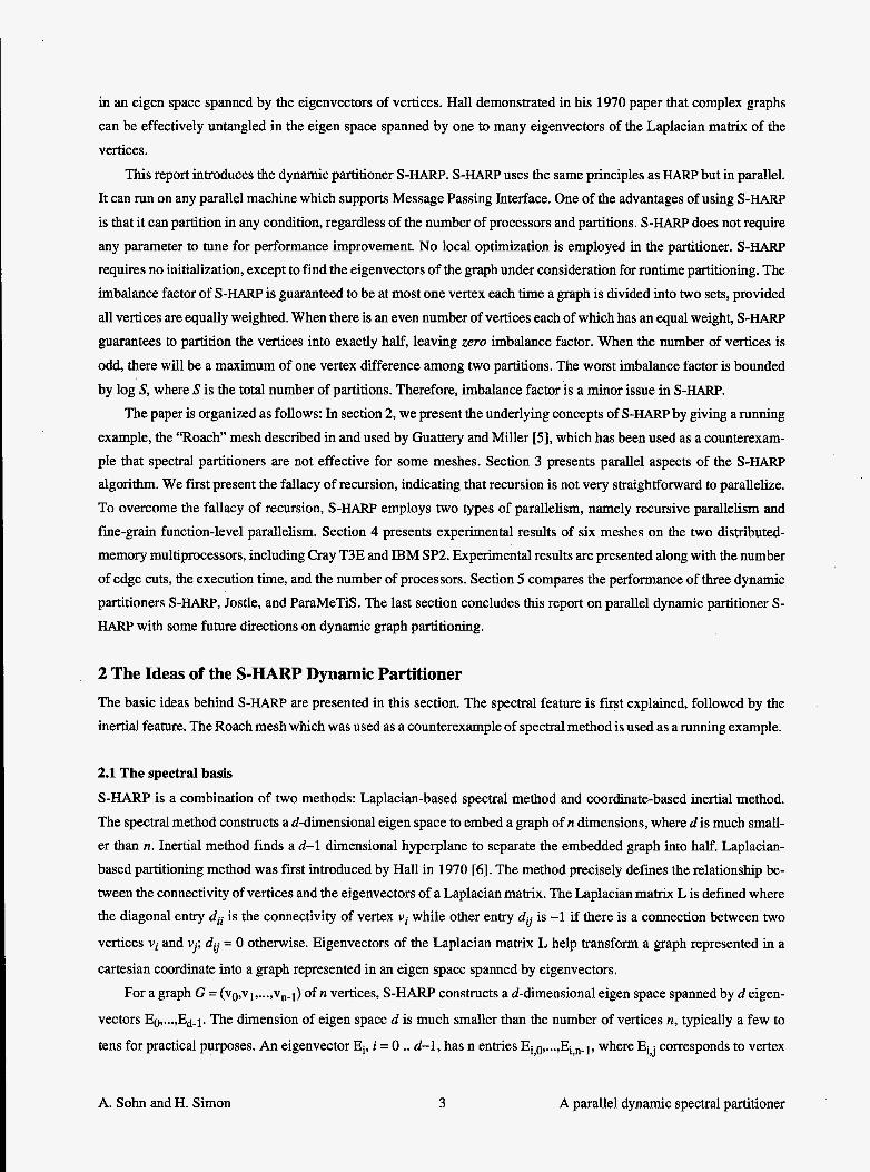
in an eigen space spanned by the eigenvectors of vertices. Hall demonstrated in his 1970 paper that complex graphs can be effectively untangled in the eigen space spanned by one to many eigenvectors of the Laplacian matrix of the vertices.

This report introduces the dynamic partitioner S-HARP. S-HARP uses the same principles as HARP but in parallel. It can run on any parallel machine which supports Message Passing Interface. One of the advantages of using S-HARP

is that it can partition in any condition, regardless of the number of processors and partitions. S-HARP does not require any parameter to tune for performance improvement. No local optimization is employed in the partitioner. S-HARP

requires no initialization, except to find the eigenvectors of the graph under consideration for runtime partitioning. The imbalance factor of S-HARP is guaranteed to be at most one vertex each time a graph is divided into two sets, provided all vertices are equally weighted. When there is an even number of vertices each of which has an equal weight, S-HARP guarantees to partition the vertices into exactly half, leaving zero imbalance factor. When the number of vertices is odd, there will be a maximum of one vertex difference among two partitions. The worst imbalance factor is bounded by log S, where S is the total number of partitions. Therefore, imbalance factor is a minor issue in S-HARP.

The paper is organized as follows: In section 2, we present the underlying concepts of S-HARP by giving a running example, the “Roach” mesh described in and used by Guattery and Miller [ 5 ] , which has been used as a counterexample that spectral partitioners are not effective for some meshes. Section 3 presents parallel aspects of the S - w algorithm. We first present the fallacy of recursion, indicating that recursion is not very straightforward to parallelize. To overcome the fallacy of recursion, S-HARP employs two types of parallelism, namely recursive parallelism and fine-grain function-level parallelism. Section 4 presents experimental results of six meshes on the two distributed- memory multiprocessors, including Cray T3E and IBM SP2. Experimental results are presented along with the number of edge cuts, the execution time, and the number of processors. Section 5 compares the performance of three dynamic partitioners S-HARP, Jostle, and ParaMeTiS. The last section concludes this report on parallel dynamic partitioner S - HARP with some future directions on dynamic graph partitioning.

2 The Ideas of the S-HARP Dynamic Partitioner The basic ideas behind S-HARP are presented in this section. The spectral feature is f i t explained, followed by the inertial feature. The Roach mesh which was used as a counterexample of spectral method is used as a running example.

2.1 The spectral basis S-HARP is a combination of two methods: Laplacian-based spectral method and coordinate-based inertial method. The spectral method constructs a d-dimensional eigen space to embed a graph of n dimensions, where d is much smaller than n. Inertial method finds a d-1 dimensional hyperplane to separate the embedded graph into half. Laplacian- based partitioning method was first introduced by Hall in 1970 [6] . The method precisely defines the relationship between the connectivity of vertices and the eigenvectors of a Laplacian matrix. The Laplacian matrix L is defined where the diagonal entry dii is the connectivity of vertex vi while other entry dij is -1 if there is a connection between two

vertices vi and vj; do = 0 otherwise. Eigenvectors of the Laplacian matrix L help transform a graph represented in a

Cartesian coordinate into a graph represented in an eigen space spanned by eigenvectors. For a graph G = (vo,v1, ..., vn-l) of n vertices, S-HARP constructs a d-dimensional eigen space spanned by d eigen-

vectors EO,...,Ed-l. The dimension of eigen space d is much smaller than the number of vertices n, typically a few to

tens for practical purposes. An eigenvector E , i = 0 .. d-1, has n entries Ei,O,...,Ei,n-l, where Eij corresponds to vertex


V J for j = 0 ... n-1. Each eigenvector of dimension n contains information of all the n vertices in the original graph but

to a limited extent. Together with other d-1 remaining eigenvectors, a vertex can be located in the d-dimensional eigen space. To be more precise, the location of a vertex vj can be accurately defined by d eigen entries hj, ..., Ed-l,j each of

which is derived from a different eigen vector. As we have shown earlier in the sequential HARP, the location of a vertex can be more accurately defined as d increases.

The traditional argument against spectral graph partitioning is that there exists a class of graphs for which spectral partitioners are not suitable. Figure 1 shows a “roach” mesh with 16 vertices used by Guattery and Miller in [5 ] . The argument in the report is that the spectral partitioner such as S-HARP will partition the roach mesh into two sets across two antennas using the dotted line. Should this be true, the partitioner will give two partitions with three components: The top partition will have two disconnected components each of which has four vertices while the bottom partition will have a single connected component of eight vertices. This type of partitioning is highly undesirable and can often be disastrous for large graphs since the top partition has two disconnected components. Putting this into perspective,

the disconnected components can cause unnecessary communications when each partition is mapped to a processor in a multiprocessor environment. To identify if this is indeed the case for Laplacian-based partitioners, we plot the roach mesh in a 2-dimensional eigen space.

Figure l(b) shows the Laplacian matrix D for the mesh shown in Figure l(a). Again, diagonal entry dii is the de-

gree of vertex vi while other entry dii is -1 if there is a connection between two vertices vi and vj; do = 0 otherwise.

Figure l(c) shows the first three eigen vectors of the matrix D. The f i s t eigenvector which is an orthonormal vector

is discarded since it has no directional information. The second and third vectors, El and E2, have directional informa-

tion and are used for graph partitioning. The plot shown in Figure l(d) is exactly based on these two eigenvectors. The 16 vertices of the roach mesh are plotted in the two-dimensional space spanned by the two eigenvectors. The x-axis shows the second eigenvector El while the y-axis shows the third eigenvector E2. These two vectors serve as an eigen coordinate for the 16 vertices.

Given the eigen plot shown in Figure l(d), partitioning the roach graph is now straightforward. The simplest way is to partition along the first eigenvector El (x-axis); The eight vertices, 0..7, of left half will be partition 0 while the eight vertices, 8..15, of right.half will be partition 1. The vertical axis passing through x=O and orthogonal to the x-axis is all it needs to partition the graph into half. The resulting partition gives the minimal number of edge cuts while all the vertices in each partition are connected. The locations of vertices 7 and 8 are not very clear in the figure and may appear to cause a potential problem for partitioning. However, they are due to the plotting precision and are numeri- cally different. Should there be ties after the graph is partitioned into half using El , spectral partitioners will spend little time resolving such cases. The second eigenvector E2 (y-axis) will be used as a tie-breaker. Should there still be ties after using E l and E2, the fourth eigenvector E3 will be used as a tie-breaker. The example graph has no ties after the first partition using El and hence, it is not necessary to use E2 to break ties.

2.2 The inertial basis

For small meshes like the one shown in the previous section, it is clear that a single eigenvector can clearly partition a graph into two connected components with the minimal edge cuts. For meshes with many ties in the eigen space, a few additional eigenvectors are necessary to break ties that often result from numerical precision. For large complex graphs, however, it is often not obvious if partitioning using one to several eigenvectors is effective. This is where the inertial feature of S-HARP is used to further clarify the partitioning process.


0

2 3 4 5 6 7 8 9

10 11 12 13 14 15

0 1 2 3 4 5 6 7 8 9 1 0 1 1 1 2 1 3 1 4 15 1 - 1 0 0 0 0 0 0 0 0 0 0 0 0 0 0

1 - 1 2-1 0 0 0 0 0 0 0 0 0 0 0 0 0 0-1 2-1 0 0 0 0 0 0 0 0 0 0 0 0 0 0-1 2-1 0 0 0 0 0 0 0 0 0 0 0 0 0 0-1 3-1 0 0 0 0 0-1 0 0 0 0 0 0 0 0-1 3-1 0 0 0-1 0 0 0 0 0 0 0 0 0 0 - 1 3 - 1 0 - 1 0 0 0 0 0 0 0 0 0 0 0 0-1 2-1 0 0 0 0 0 0 0 0 0 0 0 0 0 0 - 1 2 - 1 0 0 0 0 0 0 0 0 0 0 0 0-1 0-1 3-1 0 0 0 0 0 0 0 0 0 0 1 1 0 0 0-1 3-1 0 0 0 0 0 0 0 0-1 0 0 0 0 0-1 3-1 0 0 0 0 0 0 0 0 0 0 0 0 0 0-1 2-1 0 0 0 0 0 0 0 0 0 0 0 0 0 0-1 2-1 0 0 0 0 0 0 0 0 0 0 0 0 0 0-1 2-1 0 0 0 0 0 0 0 0 0 0 0 0 0 0-1 1

EO El E2

Figure 1: The spectral basis of S-HARP. S-HARP separates the roach graph into two connected components using the vertical line as opposed to the report that it will partition the graph using the horizontal dotted line. The resulting partitions give the minimal edge cuts while keeping all the vertices in each partition connected.

0 1 2 3 4 5 6 7 8 9 10 11 12 13 14 15 0.250 0.250 0.250 0.250 0.250 0.250 0.250 0.250 0.250 0.250 0.250 0.250 0.250 0.250 0.250 0.250 0.447 0.401 0.314 0.193 0.053 0.015 0.004 0.001 -0.001 -0.004 -0.015 -0.053 -0.193 -0.314 -0.401 -0.447 0.347 0.294 0.196 0.069 -0.069 -0.196 -0.294 -0.347 -0.347 -0.294 -0.196 -0.069 0.069 0.1% 0.294 0.347

The main idea of inertial partitioning is to find the center of inertia of vertices and decide the partition for each vertex according to the inertial center. Inertial partitioners typically use geometric coordinate information of a mesh to find the center of inertia. S-HARP uses eigen coordinate information to do so. We continue to use the roach mesh to explain the inertial feature of S-HARP. Figure 2 illustrates how the center of inertia of the 16 vertices helps partition the vertices. Given the 16 vertices represented in the 2-d space spanned by the two eigenvectors, E l and E2, S-HARP finds a line L which separates the vertices into half (if three vectors are used, S-HARP will find a plane to separate the

A parallel dynamic spectral partitioner

% 0.3

f;,

(d) The roach mesh in the eigen space spanned by E l and E2

.3 0.1

N

t; a -0.1 > M 8 W -0.3 .-

A. Sohn and H. Simon

-% ai- 0 0 0 0 -

- @ @

8

5

Eigenvector 1 (X)

Figure 2: Inertial partitioning is to find the line L which minimizes the sum of squares of distance di, i=O.. 15.

vertices into half). The line L is computed in such a way that the sum of squares of distance di, d t , i=0..15, is min-

imized. Once the line is located, the rest is straightforward. The line M that passes through the center of inertia (x,,y,)

and is orthogonal to L separates the vertices into half. Those vertices on the right hand side are projected to partition 0 while those on the left hand side are projected to partition 1, or vice versa.

When the vertices are uniformly weighted, the partitioning is as simple as above. However, S-HARP assumes weighted vertices, Le., vertices can have different computational intensity due to mesh adaption. This adds an extra

step of sorting to the above procedure. Finding the lines L and M is the same as above in a way to minimize x d t ,

i=0..15. It can be shown that finding the line L is equivalent to finding the f i s t eigenvector of a 2x2 inertial matrix R,

derived from x dt, i=0..15 [20]. However, projection will be different since weighted vertices will be projected to L

according to their weight. A simple splitting is not possible as this weighted projection has changed the center of inertia which was originally designed for a uniform weight. The projected vertices are, therefore, sorted to find the new median. The last step divides the sorted vertices into half with respect to the new median. Or, the vertices can be divided into any desired number of partitions.

Figure 3 shows how S-HARP partitions the roach graph. Figure 3(a) indicates that the inertial line L is exactly the same as the x-axis of Figure 1 while the orthogonal line M is exactly the same as the y-axis of Figure 1. Figure 3(b) shows the vertices projected to line L. Sorting is not necessary since all the vertices have the same weight. The line M passing through the center of inertia splits the vertices into half. The right hand side, labeled partition 0, has 8 vertices, v0..v7 while the left hand side, labeled partition 1, has 8 vertices, v8..v15. The partition gives 4 edge cuts, which is the

optimal number of edge cuts for connected partitions.


M A

M A

Figure 3: Inertial partitioning: (a) finding the two lines L and M, (b) projection of vertices to L, sorting on the projected values, and splitting with respect to M. Note that projected vertices in (b) are scaled for readability.

2.3 Summary of S-HARP in the context of dynamic partitioner

The internal working of S-HARP for a graph with weighted vertices is summarized below:

(a) Find k eigenvectors of the Laplacian matrix of a graph. For practical purposes, k = 10 eigenvectors are typically used [ 19,201 regardless of the number and size of vertices. For the roach mesh where k = 2 eigen vectors are used, a separator of 1-dimensional line was used. For k = 3 three vectors, a separator of 2-dimensional plane will be needed.

(b) To prepare for finding a (k-1)-dimensional hyperplane L, compute the inertial distance of the vertices in the eigen space spanned by k eigenvectors.

(c) Find a hyperplane L. This is equivalent to finding the first eigenvector of a k x k inertial matrix R derived

from the minimization of d?, i=O..V-1 , where di is an inertial distance from vertex vi to L and Vis the num-

ber of vertices.

(d) Project individual vertices to the principal inertial direction L according to their weights. (e) Sort the vertices according to the projected values. (f) Split the sorted vertices into half by using the orthogonal line M that passes through the median point of the

principal inertial direction L.

The main objective of developing S-HARP is to dynamically partition meshes. As we stated earlier in the,introduction, a computational mesh changes at runtime due to refinement andor coarsening. S-HARP assumes that the topology of the underlying mesh remains the same but the computational intensity of each vertex changes at runtime. When a mesh is refined, some vertices will split into several vertices. This refinement can be modeled by adjusting the computational weight of the vertex which is to be refined. This adjustment of computational intensity leads to an important observation that the original eigenvectors which retain the topology of the original mesh remain the same. Since the original mesh remains the same but the vertex weights change at runtime, it is not necessary to re-compute the eigenvectors at runtime. Therefore, step (a) is performed only once for the initial mesh. The parallel partitioner discussed in the following section will be concerned only for the remaining five steps.

3 The S-HARP Parallel Dynamic Partitioner Parallel aspects of S-HARP are presented in the section. The fallacy of recursive parallelism is first presented to illustrate that recursive parallelism gives very limited speedup. The two types of parallelism used in S-HARP are described,


which are coarse-grain recursive parallelism and fine-grain function-level parallelism. As explained briefly above, S- HARP assumes the eigen vectors of the meshes are given since the topology of a mesh does not change but the computational intensity does. Since there is no change in the topology, the initial eigenvectors needed to be computed once and for all at compile time. The parallel partitioner addresses only the inertial basis.

3.1 The fallacy of recursive parallelism

Parallelization of HARP 'appears' to be simple and straightforward because HARP is recursive. A key misconception of recursion, however, is that it 'appears' to be naturally parallel. In reality, it is not highly parallel until each processor has a task to perform. Given P processors, HARP will run log S iterations to obtain S sets (or partitions). In the first iteration, there is only one task to perform. Hence one and only one among P processors is busy performing this task. This gives a poor processor utilization of UP. At the end of the first iteration, the mesh is divided into two partitions. Each partition is assigned to a processor. In the second iteration, two processors independently perform mesh parti-

tioning on the given submesh. Again, the second iteration sees only two processors busy working among P processors,

resulting again in a poor utilization of 2/P. Figure 4 shows the fallacy of recursive parallelism on eight processors with three iterations. To simplify the discussion, no communication is assumed in the figure.

Po

P1

P2

P3

P4

P5

P6

P7

1 1

I- iteration 0 iteration 1 1. iteration2 ,I - - - - c

Figure 4 Fallacy of recursive parallelism. The shaded areas indicate processors that are busy.

The shaded areas indicate processors that are busy while the hollow areas indicate processors that do nothing. It is clear from Figure 4 that iteration 1, the most time consuming step, is performed by one processor while the other seven processors do nothing. The maximum speedup based on the recursive parallelism, therefore, is bound by log P. To be more precise, the speedup based on recursive parallelism is

n - - 'sequential - n Speedup = - n log P

1 + n - l o g P + 1 'parallel l o g p

P k = 1 k = l o g P k = l

n - - 'sequential - n Speedup = - n log P

1 + n - l o g P + 1 'parallel l o g p

P k = 1 k = l o g P k = l

where n is the number of iterations. For n = log P, the speedup reduces to

log P Speedup = - logP

1

k = 1


As P becomes large, the maximum possible speedup is bound by log P. The processor utilization is also very low, as is obvious from Figure 4. It is therefore imperative that the algorithm needs parallelization other than in the task- level recursion.

inertia 1 I p roject I sort I inertia I I pr oject I sort I inertia 1 1 pr oject I sort I 4 L A L A r- iteration 0 iteration 1 iteration 2

3.2 The parallel algorithm

S-HARP exploits parallelism both in recursive and function-level. Figure 5 illustrates how S-HARP works on eight processors. Three of the five steps of S-HARP have been parallelized, which are inertial computation, projection, and sort.

PO

P1

P2

P3

P4

P5

P6

PI

Figure 5: Parallel HARP running on eight processors. The figure is not drawn to scale.

In iteration 0, all the eight processors work together to find the inertial distance of the unpartitioned vertices. This step is expensive since it involves all the unpartitioned vertices and their original eigenvectors. Each processor finds an inertial matrix of VIP vertices. The dimension of inertial matrix is fixed to 10. At the end of the computation, the P inertial matrices each of which is 10x10 are reduced to a single inertial matrix of 10x10, followed by broadcasting. The second step of finding the eigenvectors of the inertial matrix is relatively trivial (typically 1-3% of the total computation time) and hence is not parallelized. The third step, where the vertex eigen coordinates of the unpartitioned vertices are projected onto the major inertial direction, is relatively expensive and hence has been parallelized. Each processor fiids the projected coordinate of VIP vertices. Unlike in the first step where P inertial matrices are reduced to a single matrix, P vectors each of which is the size of VIP are gathered in one processor to form a vector of size V, followed again by broadcasting. Sorting is the major step in S-HARP. Bitonic sorting is used to parallelize the sorting step. In particular, a balanced bitonic sorting is used in the implementation, which always sorts the elements in an as- cending order. The final step, where the unpartitioned vertices are divided into two sets, requires a negligible amount of time and is thus not parallelized.

After the graph is partitioned into two sets, they are stored across two groups of processors. The first partition is copied to processors 0 to 3 while the second partition is copied to processors 4 to 7. This is where recursive parallelism is exploited. Two groups of processors operate independently. The group of PO..P3, or GO, partitions the first set, SO into two sets while the group of P4..P7 (or G1) partitions the second set, S1, into two sets. Within each group all processors work together to perform further partition as done in iteration 0. For example, PO..P3 perform the inertial step in parallel, exploiting fine-grain function-level parallelism. If the number of desired partitions is greater than the number of processors, all the eight processors work independently after iteration 2. Recursive parallelism is fully exploited as fine-grain parallelism is not necessary from this point on.


4 Performance of S-HARP 4.1 Serial performance

Both the serial version HARP and the parallel version S-HARP have been implemented in Message Passing Interface (MPI) [ 113 on Cray T3E and IBM SP-2. The Cray T3E-900 installed at the NERSC, Lawrence Berkeley National Lab- oratory and the IBM SP-2s installed at the NASA Ames and Langley Research Centers are used for experimentation. Six test meshes are used in this study which are listed in Table 1. A brief description of the meshes is given in [18].

SPIRAL LABARRE STRUT BARTH5 HSCTL FORD2 # of vertices V 1200 7959 14,504 30,269 31,736 100,196 #of edges E 3191 22,936 57,387 44,929 142,776 222,246

Table 1: Characteristics of the six test meshes used.

Two parameters characterize the performance of all graph partitioning algorithms: the number of cut edges C and

the total partitioning time T. The sequential HARP1.0 results are compared with the MeTiS2.0 multilevel partitioner (HARP1.0 will be released for public use in the near future). MeTiS2.0 results are drawn from the early report [18]. Since the numbers of edge cuts are the same as before, they are not repeated here. However, the improved sequential HARP version gives substantially different execution times, we compare the new execution times with MeTiS2.0. Ta- ble 2 lists the execution times of HARPl.0 and MeTiS2.0 on a single-processor SP2.

# of sets

2 4 8

16 32 64

128 256

SPIRAL I LABARRE

HARPl 0.005 0.009 0.014 0.020 0.029 0.043 0.067 0.112

0.113 0.145

MeliS2 0.10 0.22 0.33 0.50 0.70 0.90 1.18 1.56

STRUT BARTH5

HARP1 MeTiS2 HARPl MeliS2 0.050 0.19 0.105 0.28 0.097 0.42 0.203 0.60 0.146 0.65 0.305 0.88 0.196 0.92 0.408 1.21 0.249 1.22 0.513 1.59 0.306 1.65 0.623 2.08 0.376 2.17 0.745 2.70 0.465 2.87 0.887 3.29

HSCTL f0rd2

HARPl MeTiS2 HARPl MeTiS2 0.110 0.48 0.352 1.18 0.213 1.00 0.684 2.40 0.320 1.84 1.023 3.59 0.426 2.24 1.360 4.78 0.533 2.93 1.698 5.92 0.646 3.76 2.040 7.50 0.772 4.90 2.391 9.23 0.916 5.97 2.761 11.35

Table 2: Comparison of the execution times in seconds on a single-processor SP2.

Experimental results in Table 2 show that HARP1.0 performs approximately three to five times faster than MeTiS2.0. All the HARPl results are based on 10 eigenvectors.

4.2 Parallel performance

Table 3 shows the execution times for Ford2 on T3E and SP2 with 1 to 64 processors. These results are plotted in Fig- ure 6. S-HARP can now partition a mesh of over 100,000 vertices in 0.2 seconds on a 64-processor T3E.

P, # of lrocesson

1 2 4 8

16 32 64

Number of partitions S on T3E Number of partitions S on SP2

2 0.358 0.230 0.154 0.123 0.104 0.090 0.088

- 4 0.827 0.466 0.290 0.214 0.168 0.140 0.137

- 8 1.290 0.699 0.406 0.283 0.212 0.168 0.159

- 16 1.740 0.927 0.520 0.340 0.248 0.189 0.180

-

-

- 32

2.183 1.143 0.629 0.395 0.275 0.201 0.188

- -

64 2.526 1.318 0.716 0.438 0.296 0.215 0.194

- -

128 2.833 1.472 0.792 0.476 0.313 0.223 0.198

- -

256 3.117 1.617 0.866 0.513 0.330 0.230 0.202

- -

2 0.352 0.244 0.186 0.158 0.140 0.127 0.141

- -

4 0.684 0.407 0302 0.244 0.209 0.189 0.198

- -

8 1.023 0.577 0.384 0.301 0.262 0.234 0.239

-

Table 3: Partitioning times of FORD2.

- 16

1.360 0.745 0.469 0.348 0.292 0.261 0.269

- -

32 1.698 0.915 0.553 0.389 0.315 0.275 0.279

-

A. Sohn and B. Simon 10 A parallel dynamic spectral partitioner

Note the diagonal timing entries in bold. The execution times decrease gradually from the upper left comer to the lower right comer, with the exception of P = S = 2. This is a unique feature S-HARP possesses among dynamic partitioners. These entries will be used to compare with other dynamic partitioners in the later section. Figure 6 is provided to illustrate the effectiveness of S-HARP. Figure 6 shows that the execution time does not logarithmically increase as the number of partitions increases logarithmically.

h

s 1 :

.$ 8 .$ 8 0.1 W

0.01

10 (a) Ford2 on T3E

f3- P=2 P=32 -4- P=4 -B- P=64 -4- P=8

(a) on T3E with 64 processors - Ford2 100196 222246) - Bad15 (30269,44929) -8- Strut (14504,57387)

-4- Hsctl(!31736,lb776)

-€J- P=l + P=16

10

(b) on SP2 with 64 processors

1 :

10

1

0.1

(b) Ford2 on SP2

1.01 10 100 Number of partitions

Figure 6: Relation between partitions and the number of processors on T3E and SP2. The plots are in log scale.

The T3E results clearly show that the total execution time is not proportional to the number of partitions. For example, consider Figure 6(a). The bottom line which shows the results on 64 processors indicates that as the number of partitions is increased to 256 from two, the execution time has risen only slightly more than twice the time for 2 partitions, i.e., 0.088 sec to 0.202 sec. This small increase indicates that even a larger number of partitions over 256 will not cost substantial computation time. A similar pattern is also seen for SP2 in Figure 6(b). When P=64, the SP2 partitioning time for 256 partitions has risen to 0.299 sec from 0.141 sec for 2 partitions, resulting in approximately twice the time for 2 partitions.

Figure 7 confirms the above observation for now four different meshes. Obtaining a very large number of partitions on 64 processors can be trivial in terms of computational cost, as shown in Figure 7. Results for all the meshes show that the partitioning times are relatively constant in spite of the logarithmic increase in the number of partitions. This relatively constant execution time is possible because the recursive parallelism is in full effect when each of the

10

h

2 1

8 a 8 0.1

.$

.- +a

w

0.01


64 processors obtains a submesh to partition. For S=256 and P=64, the first 6 iterations will see much communication to exploit functional level parallelism to overcome the fallacy of recursion (Figure 5). However, for the remaining two iterations, there will be no communication, all the processors working completely independently. Therefore, the execution times remain relatively constant once all processors each get a submesh to partition.

4.3 Scalability of S-HARP Figure 8 summarizes the scalability of S-HARP. T3E has given over 15-fold speedup on 64 processors. The speedup of 15 may be considered modest considering the parallelization efforts expended. However, graph partitioning is known to be difficult to parallelize especially when the parallel partitioners perform very fast, partitioning 100,000 vertices in 0.2 seconds. In fact, partitioners such as ParaMeTiS1.0 give very modest speedup. For the Spiral mesh, ParaMeTiS1.0 gives the speedup of 0.133/0.099 = 1.3 on 64 processors [13]. For the HSCTL mesh with V=31736, E=142776, ParaMeTiS1.0 gives the speedup of 1.81210.676 = 2.7. For the mesh Ford2, ParaMeTiS1.0 performs worse

than a single processor, giving the speedup of 0.742/0.919 = 0.81. Comparing the speedup results with ParaMeTiS1.0, S-HARP simply outperforms as it gives over 15-fold speedup. Results for the Jostle dynamic partitioner for the test meshes are not available and could not be compared in this report.

25 25 128 partitions

-+- BARTH5 (30269,44929)

'0 8 16 24 32 40 48 56 64 Number of processors

20

15

10

5

0

256 partitions

8 16 24 32 40 48 56 64 Number of processors

Figure 8: Speedup on T3E.

While S-HARP is much more scalable than other dynamic partitioners such as ParaMeTiS1.0, its 16-fold speedup on 64 processors can be still improved. The main reason for the modest speedup is due to the fact that the current version of S-HARP is not crafted for performance. The major source of improvement is the sorting step. The current version takes approximately half the time in sorting. Several solutions are currently being undertaken to reduce the sorting time and the overall parallel partitioning time.

5 Comparison of S-HARP with Other Dynamic Partitioners The performance of S-HARP is compared against two other dynamic partitioners, ParaMeTiS1.0 [9] and Jostle [21]. Jostle comes with two different versions: a multilevel version Jostle-MD and Jostle-D. Comparisons are made in terms of execution time and edge cuts. The execution results of ParaMeTiS and Jostle are provided by Leonid Oliker of FU- ACS at NASA Ames [13]. Figure 9 plots the results of S-HARP, ParaMeTiS, Jostle-MD, and Jostle-D. The x-axis indicates the number of processors and the number of partitions. For example, 64 refers that 64 processors partition the mesh into 64 sets. This restriction was due to MeTiS and Jostle since they require the number of partitions to be

A. S o h and H. Simon 12 A parallel dynamic spectral partitioner

0.20

0.15 P v

4 .d

8 0.10 .a s 3 a 0.05

0.00 1.6

- 1.2 8 v

.El 0.8 .!3

8

0.4

0.0

h

P v

SPIRAL (1200,3191) -

2 4 8 16 32 64

BARTH5 (30269,44929) n

2 4 8 16 32 64 6 1 I

Number of processors = Number of partitions

800

700

600 $ & 500 B ”0 400 4 300 z

200

100

2 4 8 1 6 3 7 M 8000

y 6000 e

% m # J El z

2000

0

BARTH5 (30269,44929) - S-Hw ParaMeTiS1.0 Jostle-MD

2 4 8 1 6 3 2 M - . 30000

FORD2 (100196,222246)

3 ParaMeTiS1.0 $0000

3

Ell0000

”015000 3

z .D

5000

2 4 8 1 6 3 2 6 4 Number of processors =Number of partitions

Figure 9: Comparison of dynamic partitioners on SP-2.

the same as the number of processors, Le., one partition per processor. S-HARP does not impose such a restriction. It can partition any number of partitions on any number of processors, as listed in Table 3.

The performance of S-HARP in terms of edge cuts is comparable to the other three. Unlike the other partitioners, S-HARP produces exactly the same solution quality, regardless of the number of processors. The performance of S- HARP in terms of edge cuts is presented in detail in [18]. S-HARP does not perform local optimization as done in ParaMeTiS and Jostle. If local optimization is employed at the expense of slightly increased computation time, the partition quality will improve to the level of MeTiS and Jostle-MD. The reason we stress “slightly” is because S-HARP

will not randomly optimize the partitions. S-HARP sorts vertices in terms of their projected locations on the dominant inertial direction in the eigen space spanned by the vertices. Local optimization will be performed where the vertices


are divided into two sets since errors come mostly from numerical precision. Hence, local optimization in the area where there are a lot of ties due to numerical precision will likely improve the partition quality. Partition quality can also be improved by using more eigenvectors. The number of eigenvectors used in this report is 10. If the number of eigenvectors is increased to 20, the performance will improve as presented in [ 181 at the expense of increased execution time. However, we have not performed local optimization since fast execution is more important in dynamically changing computations than the highest possible partition quality.

It is clear from Figure 9 that S-HARP outperformed the other two dynamic partitioners in terms of execution time. It is often difficult to obtain high performance for a small problem since there is not much work to perform. However, the results indicate that S-HARP is six to 10 times faster than ParaMeTiS and Jostle for the very small mesh Spiral. For large meshes, S-HARP still performs three to 10 times faster than ParaMeTiS and Jostle. The performance of S-HARP

is consistent throughout different sizes of meshes. The performance of S-HARP is better when the number of processors is large. For 64 processors, S-HARP is five

times faster than ParaMeTiS and 10 times faster than Jostle. This clearly suggests that when a large number of processors is used, s-HARP can be the choice among parallel dynamic partitioners. In fact, this can be easily observed by scanning the bold diagonal entries of T3E from Table 3 which are listed below again:

*T3E: 0.230,0.290, 0.283,0.248,0.201,0.194 SP2: 0.244,0.302,0.301,0.292, 0.275,0.287

We note that the execution times gradually decrease from 0.290 sec for P=S=4 to 0.194 sec for P=S=64. This is a unique feature which only S-HARP possesses among the three dynamic partitioners. The fast nature of S-HARP together with the comparable edge-cuts is certainly a viable tool for runtime partitioning of adaptive meshes on large-scale distributed-memory multiprocessors.

6 Conclusions Runtime mesh partitioning is a critical component of computational science problems when implemented on large- scale distributed-memory multiprocessors. We have presented in this paper a parallel dynamic spectral partitioner, called S-HARP. The parallel partitioner can quickly partition realistically-sized meshes on a large number of processors while maintaining the high partition quality of Laplacian-based spectral partitioning. To demonstrate the effectiveness of S-HARP, we have selected six meshes with the size of over 100,000 vertices. S-HARP exploits parallelism in task- level recursion and function-level loop to overcome the fallacy that recursion is highly parallel. When processors do not have an individual task, function level parallelism is exploited together with recursive parallelism to improve the performance. When all processors each have a task to perform, they operate independently of one another. S-HARP consists of five steps: inertia computation, eigenvector solver, project, sorting, and split. The three most time-consuming steps of inertia, project, and sort have been parallelized. The execution times of the eigen solver and split are negligible, hence not parallelized.

S-HARP has been implemented in Message Passing Interface on two distributed-memory multiprocessors: the Cray T3E installed at NERSC of Lawrence Berkeley and the IBM SP-2s installed at NASA Ames and Langley. Ex- periments have been performed up to 64 processors of the two machines. The mesh Ford2 with 100196 vertices can now be partitioned into 256 sets in 0.2 second. The results have shown that the total execution time is not proportional


to the number of partitions. As the number of partitions has logarithmically risen to 256 from 2, the execution times on a 64-processor T3E have risen slightly more than twice, i.e., 0.088 sec to 0.202 sec. A similar pattern has been observed for other meshes. All the meshes show that the partitioning times are relatively constant in spite of the logarithmic increase in the number of partitions.

When compared with other dynamic partitioners ParaMeTiS and Jostle, S-HARP is three to 10 times faster in terms of execution time for the same meshes. The partition quality of S-HARP is also very close to that of ParaMeTiS and Jostle, or there is almost negligible difference in partition quality. When a large number of processors is used, the S- HARP performance is even more encouraging since it separates further from ParaMeTiS and Jostle in terms of execution time while maintaining a very similar partition quality. S-HARP is also much more scalable than other partitioners when the number of processors is increased to 64. S-HARP has given over 15-fold speedup while ParaMeTiS has given only a few-fold speedup.

The current version of S-HARP has been implemented in MPI for portability. A plan is currently underway to improve the performance and scalability of S-HARP. While the current MPI version is effective for programming SP- 2, it is not desirable for programming T3E. MPI employs two-sided communication constructs such as Send and Recv which are suitable for message-passing machines. Cray T3E has its own programming environment SHMEM for shared-memory machines. Unlike MPI, SHMEM uses one-sided communication constructs such as put and get. It is therefore the best if T3E is programmed in the native SHMEM programming environment. However, programming in SHMEM will lose the portability of S-HARP. To obtain scalability and at the same time maintain portability, we plan to convert the communication intensive routines, sorting, to MPI-2 constructs. MPI-2 provides one,sided communication constructs such as put and get which can be readily used in the Cray SHMEM environment with little overhead.

Acknowledgments Andrew Sohn is supported in part by the NASA JOVE Program, by travel support from USRA RIACS, and by summer support from MRJ of the NASA Ames Research Center. Andrew Sohn thanks Joseph Oliger of RIACS at NASA Ames for providing travel support and Doug Sakal of MRJ Technology Solutions at NASA Ames for providing summer support. This research used resources of the National Energy Research Scientific Computing Center, which is supported by the Office of Energy Research of the U.S. Department of Energy. The IBM SP-2s installed at the NASA Ames and Langley were used to perform experiments. The authors thank Leonid Oliker of RIACS at NASA Ames for providing some of the ParaMeTiS and Jostle data. Rupak Biswas of MRJ Technology Solutions at NASA Ames helped find the eigenvectors of the meshes. S-HARP will be made available in the near future at http://www.cs.njit.edu/sohn/harp.

References 1. Accelerated Strategic Computing Initiative (ASCI), Lawrence Livermore, Los Alamos, and Sandia National

Laboratories, http://www.llnl.gov/asci/.

2. S.T. Barnard and H.D. Simon, Fast multilevel implementation of recursive spectral bisection for partitioning unstructured problems, Concurrency: Practice and Experience 6, 1994, pp. 101-1 17.

3. T. Chan, J. Gilbert, and S . Teng. Geometric spectral partitioning. Xerox PARC Technical Report, January 1995.

4. Pedro Diniz, Steve Plimpton, Bruce Hendrickson and Robert Leland, Parallel Algorithms for Dynamically Par- titioning Unstructured Grids, Proc. 7th HAM Con$ Parallel Proc., 1995.

5. S. Guattery and G. L. Miller, On the performance of the spectral graph partitioning methods, in Proc. Sixth An-


http://www.cs.njit.edu/sohn/harp

http://www.llnl.gov/asci

nual ACM-SIAM Symposium on Discrete Algorithms, 1995, pp.233-242.

6. K. Hall, An r-dimensional quadratic placement algorithm, Management Science 17, November 1970, pp.219- 229.

7. B. Hendrickson and R. Leland, A Multilevel Algorithm for Partitioning Graphs, in Proc. Supercomputing ‘95.

8. B. Hendrickson and R. Leland, Multidimensional spectral load balancing, Report SAND93-0074, Sandia Na- tional Laboratories, Albuquerque, NM, 1993.

9. G. Karypis and V. Kumar, A fast and high quality multilevel scheme for partitioning irregular graphs, Technical Report 95-035, University of Minnesota, 1995.

10. B.W. Kernighan and S. Lin, An efficient heuristic procedure for partitioning graphs, The Bell System Technical Journal, Vol. 49, 1970, pp. 291-308.

11. Message Passing Interface Forum, MPI Message-Passing Interface Standard, Version 1.1, Technical Report, University of Tennessee, Knoxville, TN, June 1995.

12. B. Nour-Omid, A. Raefsky and G. Lyzenga, Solving Finite Element Equations on Concurrent Computers, in Parallel Computations and their Impact on Mechanics, Ed. A.K.Noor, ASME, New York, 1986, p.209.

13. L. Oliker, Personal communication on the results of ParaMeTiS1.0 and Jostle on SP2 and T3E, July 30, 1997.

14. C. W. Ou and S. Ranka, Parallel Incremental Graph Partitioning, IEEE Transactions on Parallel and Distrib- uted Systems 8, August 1997, pp.884-896.

15. 0. Port, Speed gets a whole new meaning, Business Week, April 29, 1996, pp.90-91.

16. K. Schloegel, G. Karypis, and V. Kumar, Parallel Multilevel Diffusion Schemes for Repartitioning of Adaptive Meshes, Technical Report, University of Minnesota, 1997.

17. H.D. Simon, Partitioning of unstructured problems for parallel processing, Computing Systems in Engineering, Vol. 2, 1991, pp. 135-148.

18. H. D. Simon, A. Sohn, and R. Biswas, HARP: A fast spectral partitioner, in the Ninth ACM Symposium on Par- allel Algorithms and Architectures, Newport, Rhode Island, June 1997, pp.43-52.

19. A. Sohn, R. Biswas, and H. Simon, A dynamic load balancing framework for unstructured adaptive computations on distributed-memory multiprocessors, in Proceedings of the 8th ACM Symposium on Parallel Algo- rithms and Architectures, Padua, Italy, June 1996.

20. A. Sohn and H. Simon, S-HARP: A parallel dynamic spectral partitioner, Technical Report, NJIT CIS 97-20, September 1997.

21. C. Walshaw, M. Cross, and M. Everett. Dynamic mesh partitioning: a unified optimization and load-balancing algorithm. Tech. Rep. 95/IM/06, University of Greenwich, London SE18 6PF, UK, 1995.


M98052654 I11111111 Ill 11111 lllll11111 lllll11111111111111111111111

Report Number (14) M d L - - 4/34g

'ubi. Date (11) 1998 o/ Y sponsor Code (18) 'DO<Ek I r

J C Category (1 9) U L 4 u 5 ; , 90F /EK ~ ~

DOE

S-HARP: A Parallel Dynamic Spectral Partitioner

Documents

Transcript of S-HARP: A Parallel Dynamic Spectral Partitioner