S B i of macro economic acro economic Performance a u · · 2016-01-25The NFIB Research...
59
July 2012 Michael J. Chow SMALL BUSINESS INDICATORS OF MACRO-ECONOMIC PERFORMANCE: AN UPDATE SMALL BUSINESS INDICATORS OF MACRO-ECONOMIC PERFORMANCE: AN UPDATE
Transcript of S B i of macro economic acro economic Performance a u · · 2016-01-25The NFIB Research...

July 2012
Michael J. Chow
Small BuSineSS indicatorS of
macro-economic Performance: an uPdate
Small BuSineSS indicatorS of
macro-economic Performance: an uPdate

The NFIB Research Foundation is a small business-oriented research and information organi-zation affiliated with the National Federation of Independent Business, the nation’s largest small and independent business advocacy organiza-tion. Located in Washington, DC, the Foundation’s primary purpose is to explore the policy-related problems small-business owners encounter. Its peri-odic reports include Small Business Economic Trends, Small Business Problems and Priorities, and now the National Small Business Poll. The Foundation also publishes ad hoc reports on issues of concern to small-business owners.

•Since small business produces somewhat less than one-half of private GDP and employs somewhat more than one-half of the private workforce, measures of small business economic performance should correlate closely with government-produced indicators of macroeconomic performance. The flatter structure of small firms relative to large firms also arguably means that decision-makers in small firms receive information faster than decision-makers in large firms and therefore change course more quickly, providing timelier insight into the future course of national economic activity.
•NFIB has collected data quarterly on the economic performance of small businesses and their owners’ economic expectations since 1973, nearly 40 years. These quarterly data are the basis for the analysis presented here. Collection of identical data on a monthly basis began in 1986, though the monthly numbers are not employed in this analysis. The data are published each month in Small Business Economic Trends.
•The data collected from mail surveys of NFIB member samples include small business measures of sales performance, earnings, prices, labor market conditions including job openings, hiring plans and compensation, credit conditions including credit availability and interest rates, inven-tory satisfaction and plans, planned capital outlays, expansion plans, and overall expectations.
•The analysis presents an extensive series of equations and graphs showing the capacity of small business data to forecast (predict) the course of national economic performance. They relate the former to the latter, in most cases from 1973 to 2008. Some relationships prove much stronger (better predictors) than others.
•The analysis also presents a series of “out-of-sample” forecasts from 2009 through 2011 covering part of the Great Recession and its immediate aftermath. The results are effectively free (not updated quarterly) forecasts of economic activity for one of the most tumultuous periods in American economic history.
•The headline NFIB Optimism Index, an equally-weighted index of ten NFIB survey measures, does a reasonable job of predicting changes in quarterly real GDP and final sales to private domestic purchasers. Out-of-sample forecasts of real GDP growth for 2009:Q1 through 2011:Q4 are consistent with the view that the small business sector lagged performance of the large business sector and the broader economy since the Great Recession began.
•The NFIB labor market measures do an admirable job predicting changes in both private sector employment and the unemployment rate.
•The consistently best small business forecasts are of price changes. The NFIB price measures do an excellent job predicting changes in the Consumer Price Index (CPI) and the Personal Consumption Expenditures (PCE) index. However, they have difficulty predicting movements in “core” measures of CPI or PCE.
•Large, capital-intensive businesses make the lion’s share of inventory purchases and capital investments in the United States. Still, NFIB measures explain a reasonably large share of the changes in private business inventories, a notoriously volatile number, and measures of fixed private investment.
executive Summary

•The relative interest rate paid by small business owners and small business credit “tightness” are strongly correlated with the federal funds rate and the yields on common government debt securities.
•The NFIB Optimism Index outperforms both the Conference Board’s Consumer Confidence Index and the University of Michigan’s Index of Consumer Sentiment as a predictor of changes in real GDP.

taBle of contentS
Introduction . . . . . . . . . . . . . . . . . . . . . . . . . . . . . . . . . . . . . . . . . . . . . . . . . . . . . . . . . . . . . . . 1
Real GDP Growth . . . . . . . . . . . . . . . . . . . . . . . . . . . . . . . . . . . . . . . . . . . . . . . . . . . . . . . . . . 4
Employment, Unemployment, and Labor Markets . . . . . . . . . . . . . . . . . . . . . . . . . . . . . . . . . 12Employment. . . . . . . . . . . . . . . . . . . . . . . . . . . . . . . . . . . . . . . . . . . . . . . . . . . . . . . . . . . . 13Unemployment . . . . . . . . . . . . . . . . . . . . . . . . . . . . . . . . . . . . . . . . . . . . . . . . . . . . . . . . . 14Labor Compensation . . . . . . . . . . . . . . . . . . . . . . . . . . . . . . . . . . . . . . . . . . . . . . . . . . . . . 16
Inflation . . . . . . . . . . . . . . . . . . . . . . . . . . . . . . . . . . . . . . . . . . . . . . . . . . . . . . . . . . . . . . . . . 18
Business Inventories . . . . . . . . . . . . . . . . . . . . . . . . . . . . . . . . . . . . . . . . . . . . . . . . . . . . . . . . 25
Capital Expenditures . . . . . . . . . . . . . . . . . . . . . . . . . . . . . . . . . . . . . . . . . . . . . . . . . . . . . . . 29
Capital Markets . . . . . . . . . . . . . . . . . . . . . . . . . . . . . . . . . . . . . . . . . . . . . . . . . . . . . . . . . . . 33
Other Indicators . . . . . . . . . . . . . . . . . . . . . . . . . . . . . . . . . . . . . . . . . . . . . . . . . . . . . . . . . . . 38
Concluding Observations . . . . . . . . . . . . . . . . . . . . . . . . . . . . . . . . . . . . . . . . . . . . . . . . . . . . 41
Appendix A. Small Busines Economic Survey . . . . . . . . . . . . . . . . . . . . . . . . . . . . . . . . . . . . . 42
Appendix B. Notes Regarding Model Specification and Selection. . . . . . . . . . . . . . . . . . . . . . 46
Appendix C. Notes Regarding Time Series Analysis. . . . . . . . . . . . . . . . . . . . . . . . . . . . . . . . 47
Appendix D. Augmented Dickey-Fuller Test Results . . . . . . . . . . . . . . . . . . . . . . . . . . . . . . . 49
Appendix E. Granger Causality Test Results and Forecast Analysis . . . . . . . . . . . . . . . . . . . . 51

1 |
Sm
all B
usin
ess
Indi
cato
rs o
f M
acro
-eco
nom
ic P
erfo
rman
ce: A
n U
pdat
e
The National Federation of Independent Busi-ness (NFIB) began conducting economic surveys of its membership in 1973.1,2 Since that time, a virtually identical three-page questionnaire has been mailed to a sample of NFIB’s small business owner members on a regular basis, thereby preserving the compara-bility of the data series over time which now covers nearly 40 years. A copy of the current questionnaire is included in Appendix A.
From October of 1973 through 1985, a random sample of the NFIB membership list was selected, and a survey form was mailed to them on the first day of every quarter. This mailing was followed by a second about ten days later. Since January 1986, the same procedure has been followed monthly rather than quarterly. Responses are collected for about 25 days, and duplicates are purged. The yield averages about 1,850 responses in the first month of each quarter, and about 660
responses in each of the following two months, reflecting the difference in sample sizes used in the first and subsequent months in the quarter. Response rates have ranged over time from 18 percent to 33 percent, the former more char-acteristic of the early years and the latter of more recent times. A monthly report based on the findings from the survey, Small Busi-ness Economic Trends, is available from NFIB in both electronic and printed forms.3
Many private forecasters as well as govern-ment agencies use these small business survey data to obtain a better understanding of emerging trends in the economy. The list of government entities that follow the NFIB data include the Council of Economic Advisers and the Congressional Oversight Panel for the Troubled Asset Relief Program, among others.4 Of interest to followers of the NFIB data set is its predictive power with respect to economic trends in the broader economy.
introduction
“Today brings the most important business survey—if not the most impor-tant economic release—of the month. The NFIB survey of smaller busi-nesses spotted the recession coming a year ahead of the ISM manufactur-ing survey, and its failure to recover properly, even as the ISM rebounded strongly, explains why the overall performance of the economy has been so sluggish over the past couple of years.”
– Ian Shepherdson, Chief U.S. Economist, High Frequency Economics, February 14, 2012
1 A description of the origin and content of NFIB’s economic survey can be found in: William J. Dennis, Jr., and Wil-
liam C. Dunkelberg, “Small Business Economic Trends: A Quarter Century Longitudinal Data Base of Small Business
Economic Activity,” Databases for the Study of Entrepreneurship, (ed.) Jerome A. Katz, JAI, New York, 2000.2 In the early 1980s, responsibility for the survey was technically transferred from NFIB to the NFIB Research Foundation.3 Electronic versions of Small Business Economic Trends are available at www.nfib.com/research-foundation/surveys/
small-business-economic-trends.4 See, for example:
The 2011 Economic Report of the President, transmitted to the Congress February 2011 together with the annual
report of the Council of Economic Advisers, United States Government Printing Office, Washington: 2011.
Small Business Trends, Policy and Supervisory Studies, Federal Reserve Bank of Atlanta, May 2011.
“The Small Business Credit Crunch and the Impact of the TARP,” May Oversight Report, Congressional Oversight
Panel, submitted under Section 125(b)(1) of Title 1 of the Emergency Economic Stabilization Act of 2008, Pub. L. No.
110-343, 13 May 2010.
2 |
Sm
all B
usin
ess
Indi
cato
rs o
f M
acro
-eco
nom
ic P
erfo
rman
ce: A
n U
pdat
eThe last comprehensive, published analysis assessing the predictive ability of these data was released in 2003.5 This monograph builds upon the 2003 analysis not only by incorpo-rating updated (and longer) time series, ones which include the unsettling Great Reces-sion and its aftermath, but also by employing econometric techniques intended specifically for time series analysis. In general, regressions are run using NFIB data series starting from the earliest date possible through 2008:Q4 with more recent segments of data series being left out to allow for out-of-sample forecasting analysis. The regressions demonstrate how well the estimated models presented perform in predicting highly visible measures of macro-economic activity like real GDP growth, unem-ployment, inflation, and investment during the depth and aftermath of the Great Recession.
Because small firms make up such a large fraction of the total economy, it is logical to look to indicators of their collective economic health as reliable indicators of the broader economy’s performance.6 This argument is reinforced by the notion that the same basic economic forces impact all firms, large or small. Federal Reserve policy, tax-based fiscal policy, shifts in consumer spending, for example, all affect businesses of every size, although the particular effects of policies and the chan-nels through which they propagate may differ for small and large businesses. The sectoral composition of “large” and “small” firms does differ, with the large firm sector being domi-nated by industries like manufacturing, and the small firm sector being dominated by construc-tion and many services. Large firms are heavily involved in international trade, while small firms are domestically focused. These differ-
ences help explain why from time to time, the economic fortunes of large and small firms collectively diverge. Such divergences weaken the predictive power of small-business-based indicators toward macroeconomic variables. But as this monograph will show, small-busi-ness-based survey indicators remain very useful for economic analysis even when the fortunes of large and small firms diverge, let alone when in accord with data generated from large firms.7
The NFIB membership reasonably reflects the small business population but is not a representative sample of it.8 For example, members tend to be older and over-repre-sented in the Midwestern, Plains, and Moun-tain states. However, the membership’s representativeness of the overall small business population, although desirable, is not a neces-sary condition for the NFIB survey variables to be useful forecasting instruments of aggregate economic activity. Differences between the NFIB membership and the overall small busi-ness population matter in an analysis of the NFIB survey variables’ usefulness as indicators of aggregate macroeconomic activity to the extent that (a) there are material differences between the economic performance of the NFIB membership and the broader small busi-ness population and (b) indicators of economic performance for the small business population are relatively better at predicting aggregate macroeconomic activity. Since comprehensive time series data on the economic performance of the overall small business sector are scarce, these two concerns are for practical purposes irrelevant. The test of the usefulness of the NFIB data is primarily an empirical one—do the NFIB measures provide useful informa-tion for predicting and understanding variation
5 See Dunkelberg, William C., Jonathan A. Scott, and William J. Dennis, Jr., Small Business Indicators of Macroeconomic
Activity, NFIB Research Foundation, 2003.6 According to the U.S. Small Business Administration (SBA), the “small business sector” produces half of nonfarm pri-
vate gross domestic product, employs over half of all private sector employees and generated 65 percent of the nation’s
net new jobs over the past 17 years. More information on the small business sector’s importance to the U.S. economy
and labor market is available through the SBA’s FAQ, available at http://web.sba.gov/faqs/faqindex.cfm?areaID=24.7 An argument can be made that since small firms are “flatter” organizations than large firms, owners of small firms sense
changes in economic conditions more quickly than their counterparts in large firms, making indicators of the economic
health of small firms relatively more responsive to changes in the broader economic climate than indicators reflecting the
“large business sector.”8 William C. Dunkelberg and Jonathan A. Scott, “Report on the Representativeness of the National Federation of Inde-
pendent Business Sample of Small Firms in the U.S.,” Office of Advocacy, U.S. Small Business Administration, contract
#SBA2A-0084-01, mimeo, 1983.
3 |
Sm
all B
usin
ess
Indi
cato
rs o
f M
acro
-eco
nom
ic P
erfo
rman
ce: A
n U
pdat
e
in important macroeconomic measures, the focus of this monograph. In the past, NFIB has experimented with weighting the data to match Census distributions with no signifi-cant change in the indicators. More recently, NFIB examined the impact of excluding all construction firms from the sample and again, the results were not industry dependent.
The demographic distributions of the NFIB sample have, in at least one regard, changed materially over time. Today’s busi-ness size distribution (measured by number of employees per firm) is virtually identical to that recorded in the early days of the survey. Somewhat over 40 percent in both time periods employ five or fewer workers including the owner(s); about seven percent had 40 or more employees. In contrast, industry distri-bution has changed dramatically, particularly in the construction and retail sectors. In 1973, construction firms made up 10 percent of the sample compared to 19 percent in 2011. Retail firms made up 40 percent of the sample in 1973 compared to 26 percent in 2011.
In the following sections, the predictive ability of NFIB indicators toward selected prominent macroeconomic variables of interest is quantified using time series regression anal-ysis. In some cases, ordinary least squares is the method used to quantify the relation-ship. In many instances where complications due to serial correlation are detected, a first-order autoregressive model (or AR(1) model) is used to correct for disturbances in the error terms. In certain cases where the application of an AR(1) model does not provide meaningful results, Box-Jenkins methodology is applied to develop a model that may be useful for short-term forecasting.9
It must be reemphasized that regres-sions were performed for data extending only through the fourth quarter of 2008, some three plus years prior to the publication of this monograph. Again, the reason more recent data were not included in the regressions was
so that out-of-sample forecasting accuracy using the regressions herein could be observed. Out-of-sample forecasting refers to the use of regressions estimated using historical data to predict “future”10 values of the dependent vari-able. In this monograph, forecasts for several of the estimated regression equations are gener-ated for dates 2009:Q1 through 2011:Q4, providing 12 data points of out-of-sample fore-casts that can be compared with the “actual” (or “realized”) data points.
The NFIB survey data used in this anal-ysis are collected in the first month of each quarter: January, April, July, and October. NFIB publishes one value for each quarterly value. There are no revisions. The macroeco-nomic indicators used in this analysis are the quarterly values provided by the government statistical agencies that publish them. This timing sometimes builds in an implicit “lead” of at least one to two months into a regres-sion model. For example, if the January survey predicts the dependent variable of interest, say GDP growth, in the empirical relationship on a concurrent basis, then it actually predicts the quarterly value of GDP growth for January, February, and March. If NFIB data lead by one quarter, then the January survey anticipates the second quarter (representing April, May, and June) GDP growth value, an implicit lead of up to five months.
Leads are not formally denoted in the text. Instead, their chronological counterpart, lags, are denoted throughout the text by negative subscripts on the lagging variables. A subscript of “-1” means that the subscripted variable lags the reference period, usually referred to as
“time” or “period” t, by one time period (in the case of this analysis, one quarter). Similarly, a subscript of “-n” means that the subscripted variable lags the reference period by n time periods. For example, the term x-2 refers to the variable x lagged by two time periods (quarters, for current purposes) from the reference period.
9 For more information on autoregressive models and Box-Jenkins methodology, please refer to the appendix on time
series analysis.10 The term “future” here refers to time periods which extend beyond the end of the time series used to estimate the
regression equation.

4 |
Sm
all B
usin
ess
Indi
cato
rs o
f M
acro
-eco
nom
ic P
erfo
rman
ce: A
n U
pdat
e
real GdP Growth
This section explores the predictive ability of key measures in the NFIB data set toward gross domestic product (GDP). In particular, the NFIB survey’s headline Optimism Index and several of its components are shown to hold considerable explanatory power toward quarter-to-quarter changes in real GDP growth.11 Variables from the NFIB data set are also shown to hold substantial predictive power toward changes in final sales.
Gross domestic product is the broadest measure of economic activity and also, perhaps, the most closely followed. Three definitions of GDP exist. The most commonly used defi-nition is the value of final goods and services produced in the economy during a given period. A second, related definition is the sum of value added in the economy during a given period. The third definition of GDP is the sum of incomes earned in the economy during a given period.
Economists and other analysts are princi-pally interested in the change in GDP from one period to the next, as this measure provides insight into how the economy is growing over time. Positive GDP growth is associated with an expanding economy in which more goods and services are produced for consumption and investment by households and firms. Economic growth is an important concern for an expanding population since it is only through growth that full employment can be achieved without simultaneously decreasing the standard of living. Analysts generally
prefer real GDP to nominal GDP, as inflation can have a material impact on nominal GDP growth, but it is the growth in real output that is the major concern.
The most widely reported indicator from the NFIB survey is the Index of Small Busi-ness Optimism (INDEX), constructed as an equally-weighted average of 10 variables from the NFIB data set. Those variables are:
• Good Time for Business Expansion (GTEX)12
• Outlook for the Economy: Better or Worse (EBCD)13
• Net Earnings Trends: Higher or Lower (NEARN)14
• Expected Real Sales Volume: Higher or Lower (ESAL)15
• Plans to Increase/Decrease Employment (XLFCH)16
11 Throughout this analysis, regression variables are frequently represented in terms of their quarter-to-quarter percentage
change. Transforming time series variables in this manner for regression analysis has the benefit of reducing problems
common to time series analysis like serial correlation and a lack of weak dependency. A discussion regarding the selec-
tion of this functional form is provided in Appendix C on time series analysis.12 The survey question for GTEX data reads: “Do you think the next three months will be a good time for small business
to expand substantially?”13 The survey question for EBCD data reads: “About the economy in general, do you think that six months from now
general business conditions will be better than they are now, about the same, or worse?”14 The survey question for NEARN data reads: “Were your net earnings or ‘income’ (after taxes) from your business during
the last calendar quarter higher, lower, or about the same as they were for the quarter before?”15 The survey question for ESAL data reads: “Overall, what do you expect to happen to the real volume (number of units)
of goods and/or services that you will sell during the next three months?”16 The survey question for XLFCH data reads: “In the next three months, do you expect to increase or decrease the total
number of people working for you?”

5 |
Sm
all B
usin
ess
Indi
cato
rs o
f M
acro
-eco
nom
ic P
erfo
rman
ce: A
n U
pdat
e
• Job Openings Not Able to Fill (NJOBOP)17
• Current Inventory Satisfaction: Too High or Low (INVSAT)18
• Planned Inventory Change: Increase or Decrease (INVPLN)19
• Expected Change in Credit Market Conditions: Easier or Harder (XCRED)20
• Planned Capital Expenditures (CXPLAN)21
The INDEX includes mostly forward-looking measures of owner expectations and plans for sales, employment, inventory, credit, investment, and business conditions, as well as the trend in earnings growth and inven-tory satisfaction, which are potentially good predictors of future economic activity. Most of the questions used to construct the INDEX are symmetric, such as whether the owner expects the economy to be “better” or “worse” in the next six months or plans to “increase” or “decrease” the total number of people working for the firm. For these seven ques-tions, a “balance” variable (or diffusion index) is formed by subtracting the percent of unfa-vorable responses (“worse,” “decrease”) from the favorable responses (“better,” “increase”) to provide a net percent. For the other three questions, only the percent of owners offering an affirmative answer is included (for example, the percent planning capital spending or reporting that the current period
is a good time for small business expan-sion). Some variables have strong seasonal patterns, such as hiring plans. Others have little or none, such as capital spending plans or expected credit conditions. All 10 variables are seasonally adjusted and equally weighted. The INDEX is computed as the sum of the 10 seasonally adjusted components plus 100 to prevent the INDEX from becoming negative. The INDEX is based to its average value in 1986 (1986 = 100), the middle of the 1980s expansion and the beginning of the monthly NFIB time series.
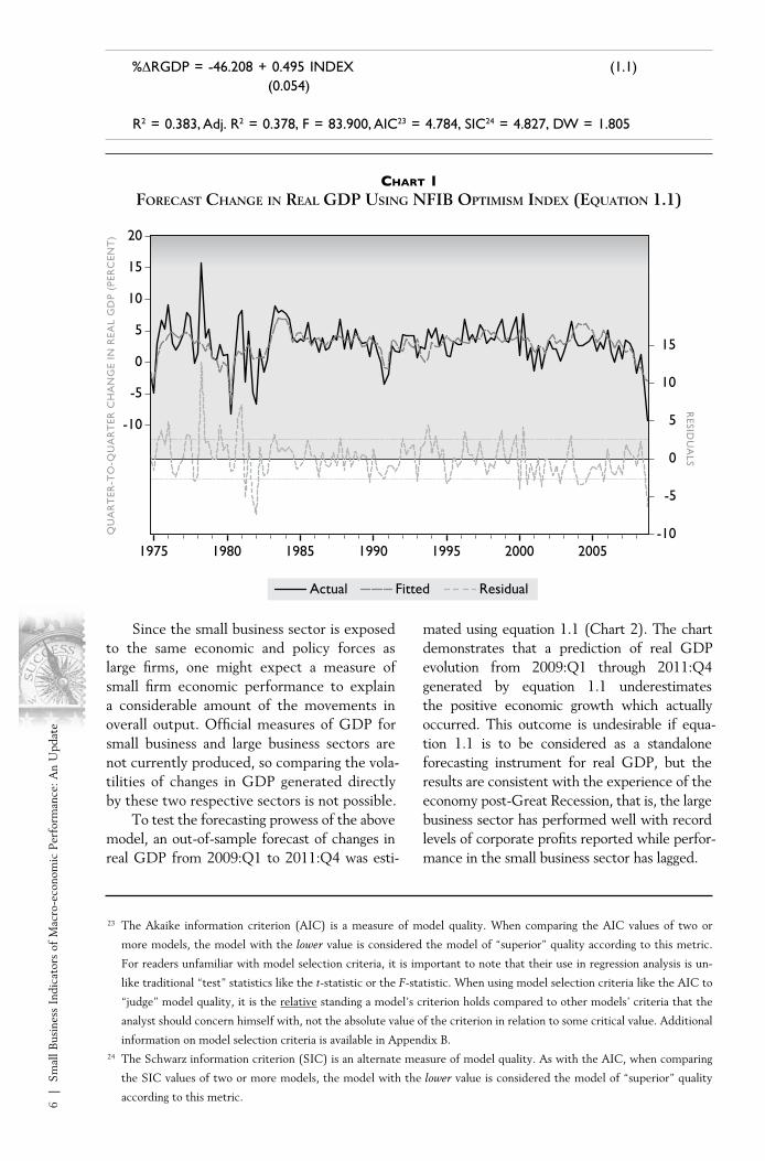
As a broad measure of economic senti-ment for one-half of the private economy, the INDEX can be expected to hold substantial explanatory power for changes in aggregate real output. The GDP measure used to assess the INDEX’s explanatory power is the quarter-to-quarter percentage change in real GDP (%∆RGDP). A simple regression of %∆RGDP on INDEX shows that INDEX does a fair job of predicting %∆RGDP, explaining 38.3 percent of the quarter-to-quarter changes (Equation 1.1).22 The slope coefficient value (0.495) is of the correct sign, since stronger performance in the small business sector (higher INDEX values) should be correlated with more robust GDP growth. The coefficient is also statisti-cally significant at the 0.05 level (p = 0.000). The model tends to do a better job predicting movements in GDP following 1982, a period of time when the GDP series was considerably less volatile (until the 2007/8 financial crisis) compared to the late 1970s to early 1980s era.
17 The survey question for NJOBOP data reads: “Do you have any job openings that you are not able to fill right now?”18 The survey question for INVSAT data reads: “At the present time, do you feel your inventories are too large, about
right, or inadequate?”19 The survey question for INVPLN data reads: “Looking ahead to the next three to six months, do you expect, on balance,
to add to your inventories, keep them about the same, or decrease them?”20 The survey question for XCRED data reads: “Do you expect to find it easier or harder to obtain your required financing
during the next three months?”21 The surveys began in October, 1973. This question was added a year later and consequently, the INDEX is available
from 1974:4 with this question included. The survey question for CXPLAN data reads: “Looking ahead to the next
three to six months, do you expect to make any capital expenditures for plant and/or physical equipment?”22 All regressions presented in this analysis were estimated using quarterly data beginning with the earliest recorded entry
for the associated NFIB data series and ending with 2008:Q4. Data from 2009:Q1 onward were omitted to allow for
the analysis of out-of-sample forecasting accuracy.
6 |
Sm
all B
usin
ess
Indi
cato
rs o
f M
acro
-eco
nom
ic P
erfo
rman
ce: A
n U
pdat
e
Chart 1forecaSt chanGe in real GdP uSinG nfiB oPtimiSm index (equation 1.1)
23 The Akaike information criterion (AIC) is a measure of model quality. When comparing the AIC values of two or
more models, the model with the lower value is considered the model of “superior” quality according to this metric.
For readers unfamiliar with model selection criteria, it is important to note that their use in regression analysis is un-
like traditional “test” statistics like the t-statistic or the F-statistic. When using model selection criteria like the AIC to
“judge” model quality, it is the relative standing a model’s criterion holds compared to other models’ criteria that the
analyst should concern himself with, not the absolute value of the criterion in relation to some critical value. Additional
information on model selection criteria is available in Appendix B. 24 The Schwarz information criterion (SIC) is an alternate measure of model quality. As with the AIC, when comparing
the SIC values of two or more models, the model with the lower value is considered the model of “superior” quality
according to this metric.
Since the small business sector is exposed to the same economic and policy forces as large firms, one might expect a measure of small firm economic performance to explain a considerable amount of the movements in overall output. Official measures of GDP for small business and large business sectors are not currently produced, so comparing the vola-tilities of changes in GDP generated directly by these two respective sectors is not possible.
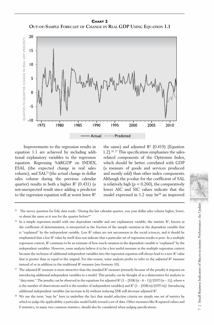
To test the forecasting prowess of the above model, an out-of-sample forecast of changes in real GDP from 2009:Q1 to 2011:Q4 was esti-
mated using equation 1.1 (Chart 2). The chart demonstrates that a prediction of real GDP evolution from 2009:Q1 through 2011:Q4 generated by equation 1.1 underestimates the positive economic growth which actually occurred. This outcome is undesirable if equa-tion 1.1 is to be considered as a standalone forecasting instrument for real GDP, but the results are consistent with the experience of the economy post-Great Recession, that is, the large business sector has performed well with record levels of corporate profits reported while perfor-mance in the small business sector has lagged.
QU
AR
TER
-TO
-QU
AR
TER
CH
AN
GE
IN R
EAL
GD
P (P
ERC
ENT
)
RESID
UA
LS
-10
-5
0
5
10
15
-10
-5
0
5
10
15
20
1975 1980 1985 1990 1995 2000 2005
ResidualActual Fitted
%∆RGDP = -46.208 + 0.495 INDEX (1.1) (0.054)
R2 = 0.383, Adj. R2 = 0.378, F = 83.900, AIC23 = 4.784, SIC24 = 4.827, DW = 1.805
7 |
Sm
all B
usin
ess
Indi
cato
rs o
f M
acro
-eco
nom
ic P
erfo
rman
ce: A
n U
pdat
e
Chart 2out-of-SamPle forecaSt of chanGe in real GdP uSinG equation 1.1
25 The survey question for SAL data reads: “During the last calendar quarter, was your dollar sales volume higher, lower,
or about the same as it was for the quarter before?”26 In a simple regression model with one dependent variable and one explanatory variable, the statistic R2, known as
the coefficient of determination, is interpreted as the fraction of the sample variation in the dependent variable that
is “explained” by the independent variable. Low R2 values are not uncommon in the social sciences, and it should be
emphasized that a low R2 value by itself does not indicate that a particular set of regression results is poor. In a multiple
regression context, R2 continues to be an estimate of how much variation in the dependent variable is “explained” by the
independent variables. However, some analysts believe it to be a less useful measure in the multiple regression context
because the inclusion of additional independent variables into the regression equation will always lead to a new R2 value
that is greater than or equal to the original. For this reason, some analysts prefer to refer to the adjusted R2 measure
instead of or in addition to the traditional R2 measure (see footnote 10).27 The adjusted R2 measure is more attractive than the standard R2 measure primarily because of the penalty it imposes on
introducing additional independent variables to a model. This penalty can be thought of as a disincentive for analysts to
“data mine.” The penalty can be observed in the equations for adjusted R2 (1 – [SSR/(n – k – 1)]/[SST/(n – 1)], where n
is the number of observations and k is the number of independent variables) and R2 (1 – (SSR/n)/(SST/n)). Introducing
additional independent variables (an increase in k) without reducing SSR will decrease adjusted R2.28 We use the term “may be” here to underline the fact that model selection criteria are simply one set of metrics by
which to judge the applicability a particular model holds toward a set of data. Other measures like R-squared values and
F-statistics, to name two common statistics, should also be considered when judging specifications.
Actual Predicted
QU
AR
TER
-TO
-QU
AR
TER
CH
AN
GE
IN R
EAL
GD
P (P
ERC
ENT
)
-10
-5
0
5
10
15
20
1975 1980 1985 1990 1995 2000 2005 2010
Improvements to the regression results in equation 1.1 are achieved by including addi-tional explanatory variables to the regression equation. Regressing %∆RGDP on INDEX, ESAL (the expected change in real sales volume), and SAL25 (the actual change in dollar sales volume during the previous calendar quarter) results in both a higher R2 (0.431) (a not-unexpected result since adding a predictor to the regression equation will at worst leave R2
the same) and adjusted R2 (0.419) [Equation 1.2].26, 27 This specification emphasizes the sales-related components of the Optimism Index, which should be better correlated with GDP (a measure of goods and services produced and mostly sold) than other index components. Although the p-value for the coefficient of SAL is relatively high (p = 0.260), the comparatively lower AIC and SIC values indicate that the model expressed in 1.2 may be28 an improved
8 |
Sm
all B
usin
ess
Indi
cato
rs o
f M
acro
-eco
nom
ic P
erfo
rman
ce: A
n U
pdat
e
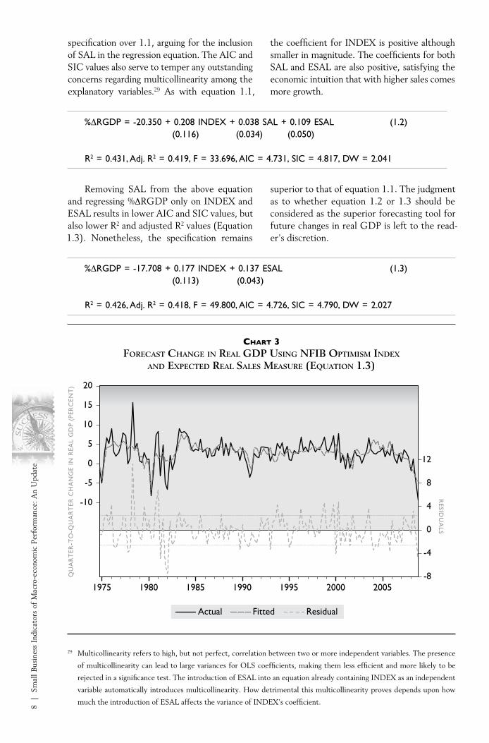
Removing SAL from the above equation and regressing %∆RGDP only on INDEX and ESAL results in lower AIC and SIC values, but also lower R2 and adjusted R2 values (Equation 1.3). Nonetheless, the specification remains
superior to that of equation 1.1. The judgment as to whether equation 1.2 or 1.3 should be considered as the superior forecasting tool for future changes in real GDP is left to the read-er’s discretion.
specification over 1.1, arguing for the inclusion of SAL in the regression equation. The AIC and SIC values also serve to temper any outstanding concerns regarding multicollinearity among the explanatory variables.29 As with equation 1.1,
the coefficient for INDEX is positive although smaller in magnitude. The coefficients for both SAL and ESAL are also positive, satisfying the economic intuition that with higher sales comes more growth.
%∆RGDP = -20.350 + 0.208 INDEX + 0.038 SAL + 0.109 ESAL (1.2) (0.116) (0.034) (0.050)
R2 = 0.431, Adj. R2 = 0.419, F = 33.696, AIC = 4.731, SIC = 4.817, DW = 2.041
%∆RGDP = -17.708 + 0.177 INDEX + 0.137 ESAL (1.3) (0.113) (0.043)
R2 = 0.426, Adj. R2 = 0.418, F = 49.800, AIC = 4.726, SIC = 4.790, DW = 2.027
Chart 3forecaSt chanGe in real GdP uSinG nfiB oPtimiSm index
and exPected real SaleS meaSure (equation 1.3)
QU
AR
TER
-TO
-QU
AR
TER
CH
AN
GE
IN R
EAL
GD
P (P
ERC
ENT
)
RESID
UA
LS
-8
-4
0
4
8
12
-10
-5
0
5
10
15
20
1975 1980 1985 1990 1995 2000 2005
ResidualActual Fitted
29 Multicollinearity refers to high, but not perfect, correlation between two or more independent variables. The presence
of multicollinearity can lead to large variances for OLS coefficients, making them less efficient and more likely to be
rejected in a significance test. The introduction of ESAL into an equation already containing INDEX as an independent
variable automatically introduces multicollinearity. How detrimental this multicollinearity proves depends upon how
much the introduction of ESAL affects the variance of INDEX’s coefficient.
9 |
Sm
all B
usin
ess
Indi
cato
rs o
f M
acro
-eco
nom
ic P
erfo
rman
ce: A
n U
pdat
e
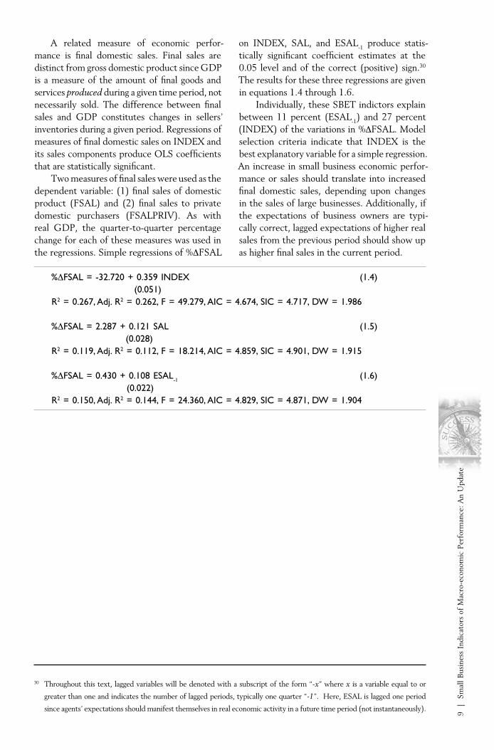
A related measure of economic perfor-mance is final domestic sales. Final sales are distinct from gross domestic product since GDP is a measure of the amount of final goods and services produced during a given time period, not necessarily sold. The difference between final sales and GDP constitutes changes in sellers’ inventories during a given period. Regressions of measures of final domestic sales on INDEX and its sales components produce OLS coefficients that are statistically significant.
Two measures of final sales were used as the dependent variable: (1) final sales of domestic product (FSAL) and (2) final sales to private domestic purchasers (FSALPRIV). As with real GDP, the quarter-to-quarter percentage change for each of these measures was used in the regressions. Simple regressions of %∆FSAL
on INDEX, SAL, and ESAL-1 produce statis-tically significant coefficient estimates at the 0.05 level and of the correct (positive) sign.30 The results for these three regressions are given in equations 1.4 through 1.6.
Individually, these SBET indictors explain between 11 percent (ESAL-1) and 27 percent (INDEX) of the variations in %∆FSAL. Model selection criteria indicate that INDEX is the best explanatory variable for a simple regression. An increase in small business economic perfor-mance or sales should translate into increased final domestic sales, depending upon changes in the sales of large businesses. Additionally, if the expectations of business owners are typi-cally correct, lagged expectations of higher real sales from the previous period should show up as higher final sales in the current period.
30 Throughout this text, lagged variables will be denoted with a subscript of the form “-x” where x is a variable equal to or
greater than one and indicates the number of lagged periods, typically one quarter “-1”. Here, ESAL is lagged one period
since agents’ expectations should manifest themselves in real economic activity in a future time period (not instantaneously).
%∆FSAL = -32.720 + 0.359 INDEX (1.4) (0.051)R2 = 0.267, Adj. R2 = 0.262, F = 49.279, AIC = 4.674, SIC = 4.717, DW = 1.986
%∆FSAL = 2.287 + 0.121 SAL (1.5) (0.028)R2 = 0.119, Adj. R2 = 0.112, F = 18.214, AIC = 4.859, SIC = 4.901, DW = 1.915
%∆FSAL = 0.430 + 0.108 ESAL-1 (1.6) (0.022)R2 = 0.150, Adj. R2 = 0.144, F = 24.360, AIC = 4.829, SIC = 4.871, DW = 1.904
10
| S
mal
l Bus
ines
s In
dica
tors
of
Mac
ro-e
cono
mic
Per
form
ance
: An
Upd
ate
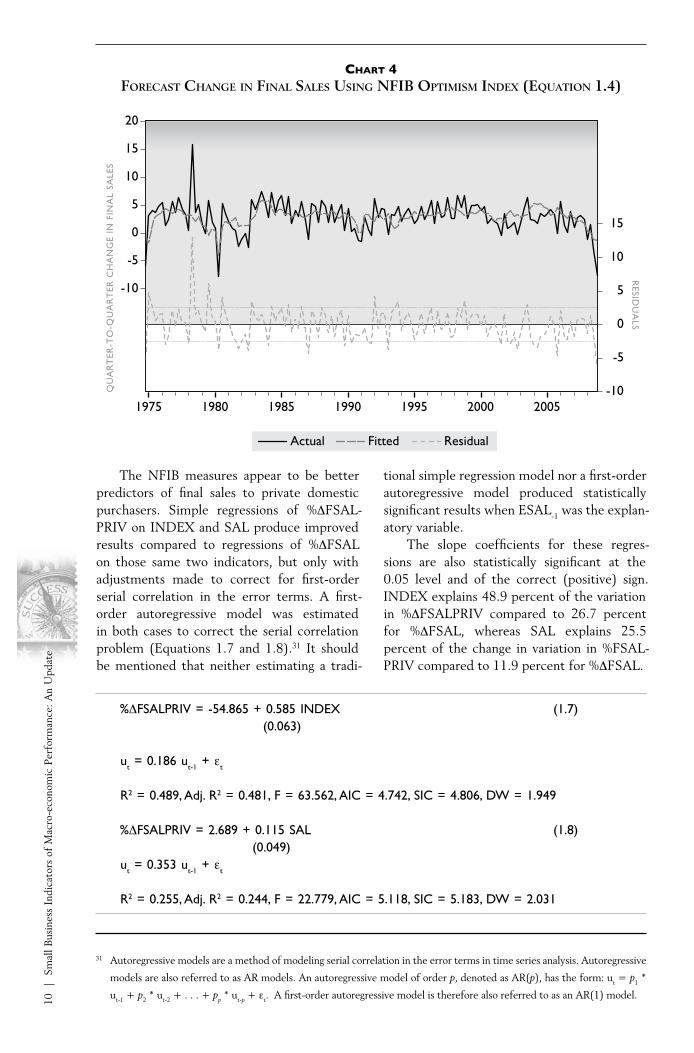
Chart 4forecaSt chanGe in final SaleS uSinG nfiB oPtimiSm index (equation 1.4)
31 Autoregressive models are a method of modeling serial correlation in the error terms in time series analysis. Autoregressive
models are also referred to as AR models. An autoregressive model of order p, denoted as AR(p), has the form: ut = p1 *
ut-1 + p2 * ut-2 + . . . + pp * ut-p + εt. A first-order autoregressive model is therefore also referred to as an AR(1) model.
The NFIB measures appear to be better predictors of final sales to private domestic purchasers. Simple regressions of %∆FSAL-PRIV on INDEX and SAL produce improved results compared to regressions of %∆FSAL on those same two indicators, but only with adjustments made to correct for first-order serial correlation in the error terms. A first-order autoregressive model was estimated in both cases to correct the serial correlation problem (Equations 1.7 and 1.8).31 It should be mentioned that neither estimating a tradi-
tional simple regression model nor a first-order autoregressive model produced statistically significant results when ESAL-1 was the explan-atory variable.
The slope coefficients for these regres-sions are also statistically significant at the 0.05 level and of the correct (positive) sign. INDEX explains 48.9 percent of the variation in %∆FSALPRIV compared to 26.7 percent for %∆FSAL, whereas SAL explains 25.5 percent of the change in variation in %FSAL-PRIV compared to 11.9 percent for %∆FSAL.
QU
AR
TER
-TO
-QU
AR
TER
CH
AN
GE
IN F
INA
L SA
LES
RESID
UA
LS
-10
-5
0
5
10
15
-10
-5
0
5
10
15
20
1975 1980 1985 1990 1995 2000 2005
ResidualActual Fitted
%∆FSALPRIV = -54.865 + 0.585 INDEX (1.7) (0.063)
ut = 0.186 ut-1 + εt
R2 = 0.489, Adj. R2 = 0.481, F = 63.562, AIC = 4.742, SIC = 4.806, DW = 1.949
%∆FSALPRIV = 2.689 + 0.115 SAL (1.8) (0.049)ut = 0.353 ut-1 + εt
R2 = 0.255, Adj. R2 = 0.244, F = 22.779, AIC = 5.118, SIC = 5.183, DW = 2.031

11
| S
mal
l Bus
ines
s In
dica
tors
of
Mac
ro-e
cono
mic
Per
form
ance
: An
Upd
ate
QU
AR
TER
-TO
-QU
AR
TER
CH
AN
GE
IN F
INA
L SA
LES
(PER
CEN
T)
RESID
UA
LS
-8
-4
0
4
8
12
-20
-10
0
10
20
1975 1980 1985 1990 1995 2000 2005
ResidualActual Fitted
Chart 5forecaSt chanGe in final Private SaleS uSinG nfiB oPtimiSm index (equation 1.7)

12
| S
mal
l Bus
ines
s In
dica
tors
of
Mac
ro-e
cono
mic
Per
form
ance
: An
Upd
ate
emPloyment, unemPloyment, and laBor marketS
This section explores the predictive ability of key measures in the NFIB data set toward private sector employment as measured by the establish-ment payroll survey and the unemployment rate. NFIB measures of changes in labor compensation at small firms are also analyzed for their predictive ability toward the employment cost index, the most comprehensive mea-sure of labor compensation available. The NFIB measures do an excellent job in predicting both changes in private employment and the unemploy-ment rate, but do not do as well predicting changes in labor compensation.
Because small firms play a critical role in the job creation process,32 the NFIB employment measures should have a strong relationship to measures of aggregate employment growth and other labor market indicators. The NFIB survey includes questions intended to measure both current and anticipated employment conditions among small businesses. Two survey measures are used to explain recent variations in employment: the net percent of owners who report expanding total employment at their firms (EMPCH)33 and the percent of owners who report at least one hard-to-fill job opening (NJOBOP). Small businesses employ half of the private sector workforce and the first survey measure (EMPCH), changes in total small business employment, should correlate with changes in total private employment.
The second measure (NJOBOP) is an indi-cator of tightness in the small business labor market. A high level of unfilled job openings indicates disequilibrium between the desired level of employment at the firm and its actual level and signals that owners are having more difficulty getting employees. Such instances generally indicate a “tight” labor market, but
may also be caused by factors other than a general shortage in labor, including regional imbalances caused by rapid growth in some areas, such as, the natural gas shale boom, and an inability of labor supply to quickly respond to changes in the labor market, such as, workers with underwater mortgages who cannot relocate. This disequilibrium between desired and actual levels of employment takes time to resolve since the hiring process is not instantaneous (collecting applications, interviewing candidates, etc.). The percent of owners reporting hard-to-fill job openings should therefore, in general, be positively correlated with employment growth and a decline in the unemployment rate.
The NFIB survey also attempts to antici-pate future changes in small business employ-ment through a third statistic which measures the net percent of owners who report plans to change total employment at their firms (XLFCH). The contribution of small firms to job creation suggests that a larger net percent of owners planning to expand total employ-ment in the months following the survey should correspond with more robust employ-ment growth in future periods.
32 According to the U.S. Small Business Administration (SBA), the small business sector employs half of all private sector
employees and generated 65 percent of the nation’s net new jobs over the past 17 years. More information on the small
business sector’s importance to the U.S. economy and labor market is available through the SBA’s FAQ, available at
http://web.sba.gov/faqs/faqindex.cfm?areaID=24.33 The survey question for EMPCH data reads: “During the last three months, did the total number of employees in your
firm increase, decrease, or stay about the same?” Respondents who report a change in employment are asked how large
the magnitude of change is. Data corresponding to the net change in small business employment was used as the inde-
pendent variable in regressions.
13
| S
mal
l Bus
ines
s In
dica
tors
of
Mac
ro-e
cono
mic
Per
form
ance
: An
Upd
ate
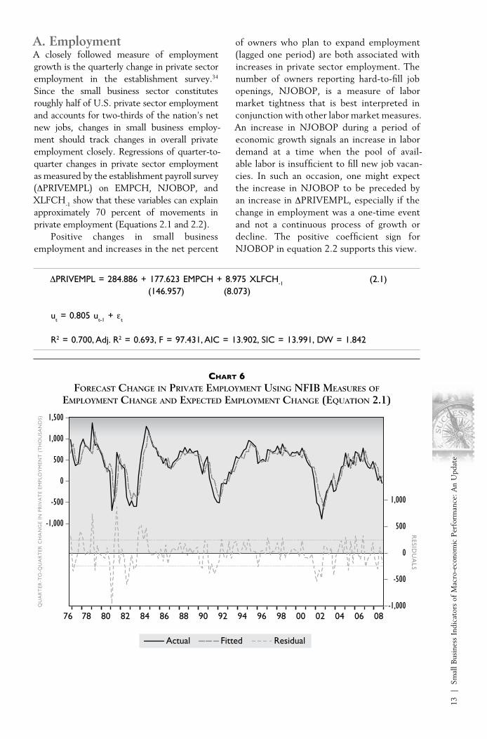
A. EmploymentA closely followed measure of employment growth is the quarterly change in private sector employment in the establishment survey.34 Since the small business sector constitutes roughly half of U.S. private sector employment and accounts for two-thirds of the nation’s net new jobs, changes in small business employ-ment should track changes in overall private employment closely. Regressions of quarter-to-quarter changes in private sector employment as measured by the establishment payroll survey (∆PRIVEMPL) on EMPCH, NJOBOP, and XLFCH-1 show that these variables can explain approximately 70 percent of movements in private employment (Equations 2.1 and 2.2).
Positive changes in small business employment and increases in the net percent
of owners who plan to expand employment (lagged one period) are both associated with increases in private sector employment. The number of owners reporting hard-to-fill job openings, NJOBOP, is a measure of labor market tightness that is best interpreted in conjunction with other labor market measures. An increase in NJOBOP during a period of economic growth signals an increase in labor demand at a time when the pool of avail-able labor is insufficient to fill new job vacan-cies. In such an occasion, one might expect the increase in NJOBOP to be preceded by an increase in ∆PRIVEMPL, especially if the change in employment was a one-time event and not a continuous process of growth or decline. The positive coefficient sign for NJOBOP in equation 2.2 supports this view.
∆PRIVEMPL = 284.886 + 177.623 EMPCH + 8.975 XLFCH-1 (2.1) (146.957) (8.073)
ut = 0.805 ut-1 + εt
R2 = 0.700, Adj. R2 = 0.693, F = 97.431, AIC = 13.902, SIC = 13.991, DW = 1.842
Chart 6forecaSt chanGe in Private emPloyment uSinG nfiB meaSureS of
emPloyment chanGe and exPected emPloyment chanGe (equation 2.1)
QU
AR
TER
-TO
-QU
AR
TER
CH
AN
GE
IN P
RIV
AT
E EM
PLO
YM
ENT
(T
HO
USA
ND
S)
RESID
UA
LS
-1,000
-500
0
500
1,000
-1,000
-500
0
500
1,000
1,500
76 78 80 82 84 86 88 90 92 94 96 98 00 02 04 06 08
ResidualActual Fitted
14
| S
mal
l Bus
ines
s In
dica
tors
of
Mac
ro-e
cono
mic
Per
form
ance
: An
Upd
ate
∆PRIVEMPL = 46.796 + 214.444 EMPCH + 16.170 NJOBOP (2.2) (141.981) (9.576)
ut = 0.777 ut-1 + εt
R2 = 0.704, Adj. R2 = 0.696, F = 98.872, AIC = 13.892, SIC = 13.981, DW = 1.894
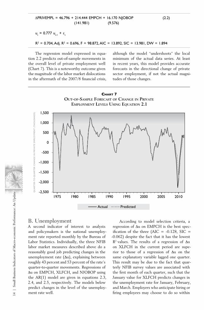
The regression model expressed in equa-tion 2.2 predicts out-of-sample movements in the overall level of private employment well (Chart 7). This is a noteworthy outcome given the magnitude of the labor market dislocations in the aftermath of the 2007/8 financial crisis,
although the model “undershoots” the local minimum of the actual data series. At least in recent years, this model provides accurate forecasts in the directional change of private sector employment, if not the actual magni-tudes of those changes.
Chart 7out-of-SamPle forecaSt of chanGe in Private
emPloyment levelS uSinG equation 2.1
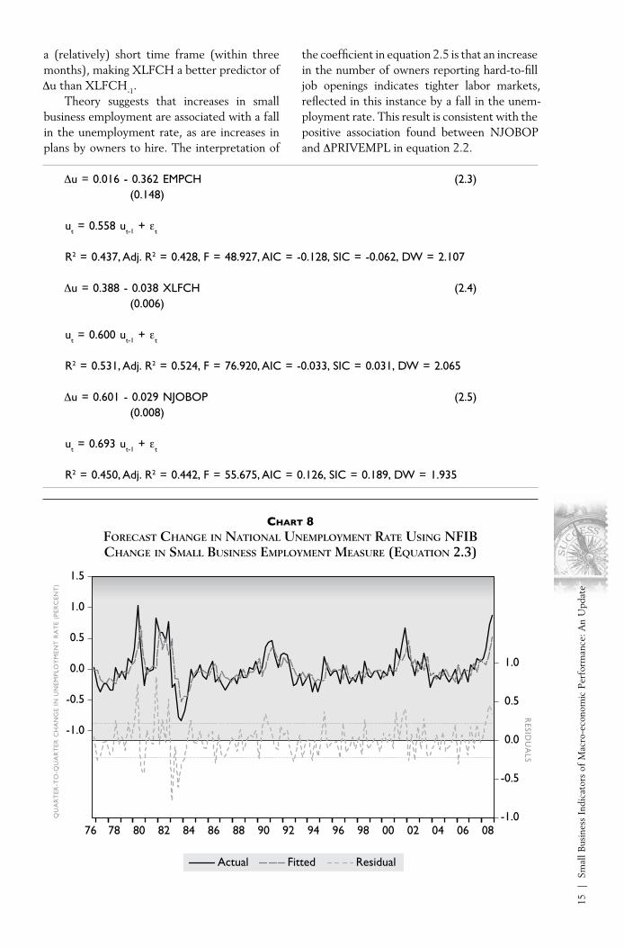
B. UnemploymentA second indicator of interest to analysts and policymakers is the national unemploy-ment rate reported monthly by the Bureau of Labor Statistics. Individually, the three NFIB labor market measures described above do a reasonably good job predicting changes in the unemployment rate (∆u), explaining between roughly 43 percent and 53 percent of the rate’s quarter-to-quarter movements. Regressions of ∆u on EMPCH, XLFCH, and NJOBOP using the AR(1) model are given in equations 2.3, 2.4, and 2.5, respectively. The models below predict changes in the level of the unemploy-ment rate well.
According to model selection criteria, a regression of ∆u on EMPCH is the best spec-ification of the three (AIC = -0.128, SIC =
-0.062) despite the fact that it has the lowest R2 values. The results of a regression of ∆u on XLFCH in the current period are supe-rior to those of a regression of ∆u on the same explanatory variable lagged one quarter. This result may be due to the fact that quar-terly NFIB survey values are associated with the first month of each quarter, such that the January value for XLFCH predicts changes in the unemployment rate for January, February, and March. Employers who anticipate hiring or firing employees may choose to do so within
Actual Predicted
QU
AR
TER
-TO
-QU
AR
TER
CH
AN
GE
IN P
RIV
AT
E EM
PLO
YM
ENT
(T
HO
USA
ND
S)
-2,500
-2,000
-1,500
-1,000
-500
0
500
1,000
1,500
1975 1980 1985 1990 1995 2000 2005 2010
15
| S
mal
l Bus
ines
s In
dica
tors
of
Mac
ro-e
cono
mic
Per
form
ance
: An
Upd
ate
a (relatively) short time frame (within three months), making XLFCH a better predictor of ∆u than XLFCH-1.
Theory suggests that increases in small business employment are associated with a fall in the unemployment rate, as are increases in plans by owners to hire. The interpretation of
the coefficient in equation 2.5 is that an increase in the number of owners reporting hard-to-fill job openings indicates tighter labor markets, reflected in this instance by a fall in the unem-ployment rate. This result is consistent with the positive association found between NJOBOP and ∆PRIVEMPL in equation 2.2.
∆u = 0.016 - 0.362 EMPCH (2.3) (0.148)
ut = 0.558 ut-1 + εt
R2 = 0.437, Adj. R2 = 0.428, F = 48.927, AIC = -0.128, SIC = -0.062, DW = 2.107
∆u = 0.388 - 0.038 XLFCH (2.4) (0.006)
ut = 0.600 ut-1 + εt
R2 = 0.531, Adj. R2 = 0.524, F = 76.920, AIC = -0.033, SIC = 0.031, DW = 2.065
∆u = 0.601 - 0.029 NJOBOP (2.5) (0.008)
ut = 0.693 ut-1 + εt
R2 = 0.450, Adj. R2 = 0.442, F = 55.675, AIC = 0.126, SIC = 0.189, DW = 1.935
Chart 8forecaSt chanGe in national unemPloyment rate uSinG nfiB chanGe in Small BuSineSS emPloyment meaSure (equation 2.3)
QU
AR
TER
-TO
-QU
AR
TER
CH
AN
GE
IN U
NEM
PLO
YM
ENT
RA
TE
(PER
CEN
T)
RESID
UA
LS
-1.0
-0.5
0.0
0.5
1.0
-1.0
-0.5
0.0
0.5
1.0
1.5
76 78 80 82 84 86 88 90 92 94 96 98 00 02 04 06 08
ResidualActual Fitted

16
| S
mal
l Bus
ines
s In
dica
tors
of
Mac
ro-e
cono
mic
Per
form
ance
: An
Upd
ate
That indicators of labor market conditions in the small business sector serve as useful predictors of the unemployment rate is by itself unremarkable, given the sector’s importance to overall employment and job creation. What is noteworthy is that it is the NFIB measures in the current period and not in previous periods which serve as useful predictors of ∆u. Unem-ployment is considered to be a lagging indicator by economists, and one might presuppose that NFIB measures lagged a period might act as
the best explanatory variables for regressions of ∆u. But, the above empirical results show this is not necessarily the case.
In a test of out-of-sample forecasting, equation 2.4 does an admirable job predicting the directional movements of actual changes in the unemployment rate, similar to equation 2.2’s reliability as a forecasting tool for direc-tional movements in changes in the level of private sector employment.
35 The survey question for PASTWAGE data reads: “Over the past three months, did you change average employee compen-
sation (wages and benefits but NOT Social Security, U.C. taxes, etc.)?”36 The survey question for PLANWAGE data reads: “Do you plan to change average employee compensation (wages and
benefits but NOT Social Security, U.C. taxes, etc.) during the next three months?”
Chart 9out-of-SamPle forecaSt of chanGe in unemPloyment rate uSinG equation 2.4
C. Labor CompensationThe major cost incurred by small business is usually labor. Overall, the path of labor costs drives the price level because firms that cannot cover labor costs will fail. Since April 1982, the NFIB survey has asked a series of questions about past and planned labor cost changes in addition to indicators of labor demand.
PASTWAGE35 is the net percent of owners reporting that they raised labor compensation in the prior three-month period. PLANWAGE36 is the net percent of owners planning to increase
labor compensation during the next three-month period. Both are seasonally adjusted. PAST-WAGE and PLANWAGE are direct measures of actual and anticipated changes in labor compen-sation (wages and benefits). Wages represent the price of labor and, as such, should vary with changes in the supply and demand for it. The two NFIB wage measures are strongly correlated not only with each other, but also with NJOBOP and XLFCH (Table 1). More vacancies and plans to increase hiring indicate tightening labor markets, which support wage increases.
Actual Predicted
QU
AR
TER
-TO
-QU
AR
TER
CH
AN
GE
IN U
NPE
MPL
OY
MEN
T R
AT
E (P
ERC
ENT
)
-1.0
-0.5
0.0
0.5
1.0
1.5
2.0
1975 1980 1985 1990 1995 2000 2005 2010

17
| S
mal
l Bus
ines
s In
dica
tors
of
Mac
ro-e
cono
mic
Per
form
ance
: An
Upd
ate
table 1 correlation matrix of nfiB laBor market and comPenSation meaSureS
The NFIB wage variables should have a positive relationship to macro measures of labor compensation, PLANWAGE with a lag and PASTWAGE in the current period. Macro measures of labor compensation are scarce and the most popular of these time series is relatively short in duration. The Employment Cost Index (ECI) is the most comprehensive measure of labor costs available, compiled by the Bureau of Labor Statistics using surveys of both private and public sectors. The headline ECI index incorporates information on wages, salaries, and benefits, but separate indices representing just wage and salary or benefits are also available. ECI data are available quar-
terly from 2001:Q1, and 2005 serves as the index’s reference year (2005 = 100).
Regressions of the quarter-to-quarter percentage change of the wage and salary index (%∆ECI) on NFIB labor compensa-tion measures indicate that PASTWAGE and PLANWAGE-1 do a relatively poor job predicting changes in the ECI (Equations 2.6, 2.7, and 2.8). The OLS coefficient for PAST-WAGE in equation 2.6 is not statistically signif-icant (p = 0.543), making equation 2.6 a poor specification. Meanwhile, simple regressions of %∆ECI on PASTWAGE and PLANWAGE-1 explain just 8.3 percent and 20.7 percent, respectively, of movements in the ECI.
%∆ECI = 0.256 - 0.009 PASTWAGE + 0.044 PLANWAGE-1 (2.6) (0.014) (0.020)R2 = 0.217, Adj. R2 = 0.161, F = 3.887, AIC = -0.596, SIC = -0.458, DW = 1.844
%∆ECI = 0.379 + 0.015 PASTWAGE (2.7) (0.009)R2 = 0.083, Adj. R2 = 0.051, F = 2.627, AIC = -0.502, SIC = -0.410, DW = 2.031
%∆ECI = 0.205 + 0.035 PLANWAGE-1 (2.8) (0.013)R2 = 0.207, Adj. R2 = 0.179, F = 7.557, AIC = -0.648, SIC = -0.555, DW = 1.877
NJOBOP XLFCH PASTWAGE PLANWAGE
NJOBOP 1.000000 XLFCH 0.874038 1.000000 PASTWAGE 0.871097 0.874673 1.000000 PLANWAGE 0.709297 0.738056 0.860684 1.000000
These disappointments aside, it is possible that the results are influenced by the small sample size of the ECI time series. The ECI series begins in 2001:Q1, providing just 32 observations for this analysis. Even if the R2
values were higher and the coefficients of the right signs in equations 2.6, 2.7, and 2.8, the small sample size would encourage caution against reading too much into the results. Revisiting this analysis once the ECI has
become a more mature time series may be a worthwhile endeavor.
Overall, the NFIB labor market indicators are highly correlated with two of three impor-tant macro labor market variables. Changes in private sector employment and the unem-ployment rate are both very well anticipated by the NFIB survey measures. Changes in worker compensation are not anticipated well by NFIB measures.
18
| S
mal
l Bus
ines
s In
dica
tors
of
Mac
ro-e
cono
mic
Per
form
ance
: An
Upd
ate
inflation
This section discusses the predictive ability of measures in the NFIB data set toward changes in various forms of inflation. The regular consumer price index (CPI), “core” consumer price index, personal consumption ex-penditure index, and GDP deflator are regressed against NFIB measures of past and planned changes in selling prices by small business owners. Using a first-order autoregressive model, the NFIB measures do an excel-lent job predicting changes in the regular CPI, the personal consumption expenditure index, and the GDP deflator. Box-Jenkins methodology can be employed to obtain a model that predicts well changes in “core” CPI.
Along with “full employment,” inflation is the major concern of economic policy. Two NFIB survey questions address this economic phenomenon in the small business sector: reported changes in average selling prices over the past three months (PASTP)37 and reported plans for raising selling prices in the next three months (PLANP).38 The variable PASTP is the percent of owners who report raising average selling prices less the percent who report lowering prices (the net percent, seasonally adjusted). PASTP should hold explanatory power toward current consumer price index changes, since price changes implemented by business owners in the three months prior to
the survey will impact price measures in the current period. In a similar fashion, PLANP, the percent of owners planning to increase average selling prices less the percent planning to reduce average selling prices, should lead CPI changes. Plans from the prior quarter should show up as changes in prices during the current period.
The two NFIB measures of price changes predict well changes in the consumer price index (Equation 3.1). Together, PLANP39 and PASTP explain 69.0 percent of the annualized percentage change in the headline CPI using a first-order autoregressive model. Price increases by owners, both actual and planned, anticipate increases in the consumer price index.
37 The survey question for PASTP data reads: “How are your average selling prices now compared to three months ago?”38 The survey question for PLANP data reads: “In the next three months, do you plan to change the average selling prices
of your goods and/or services?”39 Theory suggests that in equation 3.1 and some others that follow, PLANP should be lagged by at least one quarter. In
these several cases, practice is inconsistent with theory, as regressions containing PLANP-1 in place of PLANP gener-
ated poor results. As a general rule throughout this section, regressions containing PLANP-1 were first attempted. If the
estimated coefficients proved to be statistically insignificant, then PLANP was substituted for PLANP-1.
%∆CPI = -2.027 + 0.051 PASTP + 0.230 PLANP (3.1) (0.026) (0.051)
ut = 0.458 ut-1 + εt
R2 = 0.690, Adj. R2 = 0.683, F = 100.175, AIC = 4.124, SIC = 4.208, DW = 1.784

19
| S
mal
l Bus
ines
s In
dica
tors
of
Mac
ro-e
cono
mic
Per
form
ance
: An
Upd
ate
Chart 10forecaSt chanGe in conSumer Price index uSinG
nfiB Price meaSureS (equation 3.1)
Chart 11 shows the out-of-sample predicted versus actual values of the quarter-to-quarter change in the consumer price index using the model expressed in equation 3.1. As with the labor market models, this model also tends to accurately predict post-Great Reces-
sion directional movements in the price indices, this time with a slight lag. This will also prove to be the case with out-of-sample forecasts of changes in the personal consumption expendi-ture index and the GDP deflator, as will be shown later.
Chart 11out-of-SamPle forecaSt of chanGe in cPi uSinG equation 3.1
QU
AR
TER
-TO
-QU
AR
TER
CH
AN
GE
IN C
PI (
PER
CEN
T)
RESID
UA
LS
-12
-8
-4
0
4
8
-10
-5
0
5
10
15
20
1975 1980 1985 1990 1995 2000 2005
ResidualActual Fitted
QU
AR
TER
-TO
-QU
AR
TER
CH
AN
GE
IN C
PI (
PER
CEN
T)
-10
-5
0
5
10
15
20
1975 1980 1985 1990 1995 2000 2005 2010
Actual Predicted
20
| S
mal
l Bus
ines
s In
dica
tors
of
Mac
ro-e
cono
mic
Per
form
ance
: An
Upd
ate
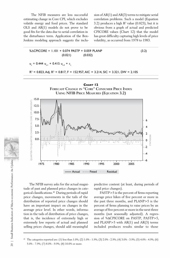
The NFIB measures are less successful estimating change in Core CPI, which excludes volatile energy and food prices. The standard OLS and AR(1) models do not prove to be good fits for the data due to serial correlation in the disturbance term. Application of the Box-Jenkins modeling approach suggests the inclu-
sion of AR(1) and AR(3) terms to mitigate serial correlation problems. Such a model (Equation 3.2) produces a high R2 value (0.823), but it is obvious from a graph of actual and predicted CPICORE values (Chart 12) that the model has great difficulty capturing high levels of price volatility, as occurred from 1978 to 1983.
%∆CPICORE = 1.101 + 0.074 PASTP + 0.059 PLANP (3.2) (0.021) (0.032)
ut = 0.444 ut-1 + 0.415 ut-3 + εt
R2 = 0.823, Adj. R2 = 0.817, F = 152.957, AIC = 3.214, SIC = 3.321, DW = 2.105
Chart 12forecaSt chanGe in “core” conSumer Price index
uSinG nfiB Price meaSureS (equation 3.2)
The NFIB survey asks for the actual magni-tude of past and planned price changes in cate-gorical classifications.40 During periods of rapid price changes, movements in the tails of the distribution of reported price changes should have an important impact on changes in the average price level. In other words, informa-tion in the tails of distribution of price changes, that is, the incidence of extremely high or extremely low reports of actual and planned selling prices changes, should add meaningful
predictive content (at least, during periods of rapid price changes).
PASTP>5 is the percent of firms reporting average price hikes of five percent or more in the past three months, and PLANP>5 is the percent of firms planning to raise prices by an average of five percent or more in the next three months (not seasonally adjusted). A regres-sion of %∆CPICORE on PASTP, PASTP>5, and PLANP>5 with AR(1) and AR(3) terms included produces results similar to those
40 The categories reported are: (1) less than 1.0%; (2) 1.0% - 1.9%; (3) 2.0% - 2.9%; (4) 3.0% - 3.9%; (5) 4.0% - 4.9%; (6)
5.0% - 7.9%; (7) 8.0% - 9.9%; (8) 10.0% or more.
QU
AR
TER
-TO
-QU
AR
TER
CH
AN
GE
IN C
OR
E C
PI (
PER
CEN
T)
RESID
UA
LS
-6
-4
-2
0
2
4
6
0.0
2.5
5.0
7.5
10.0
12.5
15.0
1975 1980 1985 1990 1995 2000 2005
ResidualActual Fitted

21
| S
mal
l Bus
ines
s In
dica
tors
of
Mac
ro-e
cono
mic
Per
form
ance
: An
Upd
ate
%∆CPICORE = 2.129 + 0.105 PHIGHER – 0.116 PLOWER (3.4) (0.026) (0.060)
ut = 0.444 ut-1 + 0.414 ut-3 + εt
R2 = 0.822, Adj. R2 = 0.817, F = 152.870, AIC = 3.215, SIC = 3.321, DW = 2.090
PASTP and PLANP do a better job antic-ipating or predicting changes in the Personal Consumption Expenditures price index (%∆PCE) than in the consumer price index (Equation 3.5). The PCE index is constructed using the CPI, the Producer Price Index, and other data sources. A key difference between the CPI and the PCE is that the CPI repre-sents a “fixed” (relatively) basket of goods whereas PCE allows the basket of goods to
change quarter to quarter. In contrast, the CPI basket is updated every two years.
Using an AR(1) model, the NFIB measures explain 78.5 percent of movements in the PCE index. The residuals are well distributed and small until 2008, when firms cut prices dramatically to reduce excessive levels of inventory created by lower consumer spending following the beginning of the finan-cial crisis.
%∆PCE = -1.541 + 0.027 PASTP + 0.202 PLANP (3.5) (0.020) (0.035)
ut = 0.678 ut-1 + εt
R2 = 0.785, Adj. R2 = 0.780, F = 164.355, AIC = 3.353, SIC = 3.438, DW = 2.000
for equation 3.2 (Equation 3.3). Increases in both PASTP>5 and PLANP>5 contribute to increases in the general price level. As before,
the model has difficulty accurately predicting periods of high price volatility.
%∆CPICORE = 0.666 + 0.041 PASTP + 0.151 PASTP>5 + 0.094 PLANP>5-1 (3.3) (0.021) (0.048) (0.048)
ut = 0.352 ut-1 + 0.460 ut-3 + εt
R2 = 0.831, Adj. R2 = 0.824, F = 127.805, AIC = 3.134, SIC = 3.263, DW = 2.077
Similar results are obtained through a regression of %∆CPICORE on the percent of firms who report raising prices in the previous three months (PHIGHER) and the percent of firms who report lowering prices
(PLOWER) [Equation 3.4]. In this model, a larger percentage of firms raising prices leads to increases in the general price level, and a larger percentage of firms lowering prices leads to decreases.

22
| S
mal
l Bus
ines
s In
dica
tors
of
Mac
ro-e
cono
mic
Per
form
ance
: An
Upd
ate
Chart 13forecaSt chanGe in PerSonal conSumPtion exPenditureS Price
index uSinG nfiB Price meaSureS (equation 3.5)
Chart 14out-of-SamPle forecaSt of chanGe in Pce index uSinG equation 3.5
QU
AR
TER
-TO
-QU
AR
TER
CH
AN
GE
IN P
CE
(PER
CEN
T)
RESID
UA
LS
-8
-6
-4
-2
0
2
4
-10
-5
0
5
10
15
1975 1980 1985 1990 1995 2000 2005
ResidualActual Fitted
QU
AR
TER
-TO
-QU
AR
TER
CH
AN
GE
IN P
CE
IND
EX (
PER
CEN
T)
-8
-4
0
4
8
12
16
1975 1980 1985 1990 1995 2000 2005 2010
Actual Predicted

23
| S
mal
l Bus
ines
s In
dica
tors
of
Mac
ro-e
cono
mic
Per
form
ance
: An
Upd
ate
%∆PCECORE = 0.854 + 0.023 PASTP – 0.049 PLANP (3.6) (0.015) (0.049)
ut = 0.970 ut-1 - 0.581 θt-1 + εt
R2 = 0.891, Adj. R2 = 0.888, F = 273.806, AIC = 2.408, SIC = 2.514, DW = 1.785
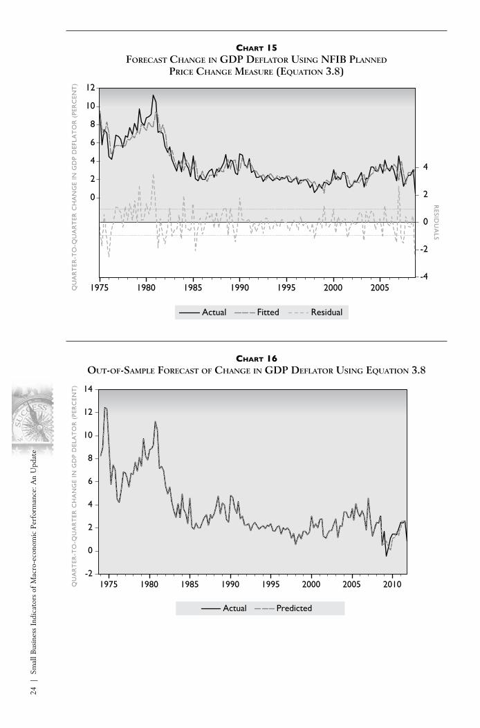
Finally, future short-term changes in the GDP deflator may be predicted accurately by PASTP or PLANP-1 with the inclusion of
AR(1) and AR(4) terms in the model (Equa-tions 3.7 and 3.8).
%∆GDPDFL = 1.942 + 0.068 PASTP (3.7) (0.014)
ut = 0.497 ut-1 + 0.332 ut-4 + εt
R2 = 0.845, Adj. R2 = 0.841, F = 239.613, AIC = 2.688, SIC = 2.773, DW = 2.035
%∆GDPDFL = 1.332 + 0.064 PLANP-1 (3.8) (0.022)
ut = 0.550 ut-1 + 0.306 ut-4 + εt
R2 = 0.830, Adj. R2 = 0.826, F = 214.344, AIC = 2.781, SIC = 2.867, DW = 2.004
Regular OLS and autoregressive models fail to accurately predict movements in the Core PCE index, which omits energy and food prices. Introducing both an AR(1) and a MA(1) term gives a model with a high degree of explanatory power (Equation 3.6).
This ARMA(1, 1) model may be useful for short-term forecasting of the Core PCE index despite the fact that the negative coefficient for PLANP runs counter to conventional economic wisdom.41
41 ARMA(p, q) models are a class of models referred to as autoregressive moving average models which include both an
autoregressive term (AR) of order p, as well as a moving average (MA) term of order q. The moving average term con-
sists of lagged values of the forecast error (not the residual), used to improve the current forecast. An MA(q) takes the
form: ut = εt +θ1 * εt-1 + θ2 * εt-2 + … + θq * εt-q. ARMA(p, q) models are frequently assembled using ARIMA (autore-
gressive integrated moving average) modeling principles (also referred to as Box-Jenkins methodology) which attempt
to construct a forecasting model using AR, MA, and integration order terms. Such models can be useful for short-term
forecasting but often lack theoretical meaning.
24
| S
mal
l Bus
ines
s In
dica
tors
of
Mac
ro-e
cono
mic
Per
form
ance
: An
Upd
ate
Chart 15forecaSt chanGe in GdP deflator uSinG nfiB Planned
Price chanGe meaSure (equation 3.8)
Chart 16
out-of-SamPle forecaSt of chanGe in GdP deflator uSinG equation 3.8
QU
AR
TER
-TO
-QU
AR
TER
CH
AN
GE
IN G
DP
DEF
LAT
OR
(PE
RC
ENT
)
RESID
UA
LS
-4
-2
0
2
4
0
2
4
6
8
10
12
1975 1980 1985 1990 1995 2000 2005
ResidualActual Fitted
QU
AR
TER
-TO
-QU
AR
TER
CH
AN
GE
IN G
DP
DEL
AT
OR
(PE
RC
ENT
)
Actual Predicted
-2
0
2
4
6
8
10
12
14
1975 1980 1985 1990 1995 2000 2005 2010

25
| S
mal
l Bus
ines
s In
dica
tors
of
Mac
ro-e
cono
mic
Per
form
ance
: An
Upd
ate
BuSineSS inventorieS
NFIB measures of inventory satisfaction and inventory changes (planned or actual) among small business owners are shown to predict well changes in overall private inventory levels as measured by the NIPA accounts.
Changes in non-farm business invento-ries are notoriously difficult to predict. These inventory changes are a function of produc-tion decisions by makers of goods throughout the economy, decisions by business owners to adjust their stock of inventories, and consumer (customer) purchases during a given period. Mismatches between inventory stock adjustments by business owners and consumer purchases can lead to large swings in inven-tories. Additionally, mismatches between the amount of goods generated by producers during a given period and the amount of new or replacement inventory desired by owners will lead to a mismatch between the planned and actual levels of inventory in future periods.
A common model in macroeconomics for examining inventory investment is the stock adjustment model, in which the desired stock of inventories depends on expected sales in the future period, the cost of holding inven-tories, the ratio of inventory to sales that is desirable for that particular type of business, and the stock on hand. Comparing the desired stock to the stock on hand produces a gap that, if positive, must be closed by additional inventory accumulation and, if negative, must
be closed by reducing inventories. The net percent of owners characterizing their current stocks as “too high” or “too low” (INVSAT) is a direct proxy for the gap between desired and actual stocks. Meanwhile, the pervasive-ness among small businesses of a gap between desired and actual inventory stocks drives the percent of owners planning to intention-ally add to (or subtract from) inventory stocks (INVPLN).
Theory suggests that inventory stocks in future periods should increase in response to situations where owners feel current stocks are low or plan to add inventory. This relation-ship is tested in equation 4.1, which relates the actual quarter-to-quarter change in overall U.S. business inventories (∆INV) as reported in the National Income and Product Accounts to the NFIB survey measures of inventory satis-faction (INVSAT), the net percent of owners reporting that current holdings are too high or too low, and inventory plans (INVPLN), the net percent of owners planning to intention-ally increase inventory holdings.42 Changes in business inventories are regressed on previous period measures of both inventory satisfaction and planned changes in inventory.
∆INV = 18.432 + 1.925 INVSAT-1 + 4.676 INVPLN-1 (4.1) (1.459) (0.873)
R2 = 0.312, Adj. R2 = 0.302, F = 31.131, AIC = 9.697, SIC = 9.760, DW = 1.145
A correlogram of the residuals obtained from this regression indicate the possible pres-ence of serial correlation. The introduction of an AR(1) term into the equation produces improved statistical performance. However, the coefficient for INVSAT-1 is now well outside the realm of statistical significance (p
= 0.6135). A regression model with INVSAT-1
and INVPLN-1 is therefore not the best model specification. Nonetheless, because of theoret-ical underpinnings, some further analysis of the results is merited. The model tracks changes in business inventories well for the first several years of the time series until 1982, after which the predicted values deviate from the actual values, generally by failing to match the vola-
42 Statistics on business inventories for the small business sector are not currently produced, so a measure of overall busi-
ness inventories is used instead.
26
| S
mal
l Bus
ines
s In
dica
tors
of
Mac
ro-e
cono
mic
Per
form
ance
: An
Upd
ate
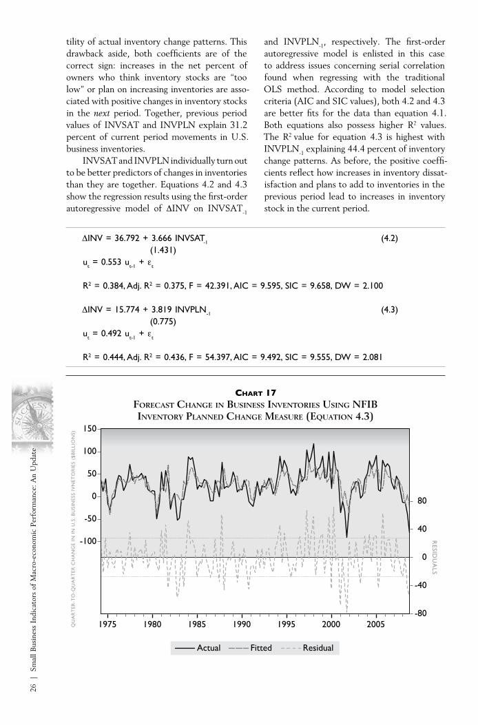
tility of actual inventory change patterns. This drawback aside, both coefficients are of the correct sign: increases in the net percent of owners who think inventory stocks are “too low” or plan on increasing inventories are asso-ciated with positive changes in inventory stocks in the next period. Together, previous period values of INVSAT and INVPLN explain 31.2 percent of current period movements in U.S. business inventories.
INVSAT and INVPLN individually turn out to be better predictors of changes in inventories than they are together. Equations 4.2 and 4.3 show the regression results using the first-order autoregressive model of ∆INV on INVSAT-1
and INVPLN-1, respectively. The first-order autoregressive model is enlisted in this case to address issues concerning serial correlation found when regressing with the traditional OLS method. According to model selection criteria (AIC and SIC values), both 4.2 and 4.3 are better fits for the data than equation 4.1. Both equations also possess higher R2 values. The R2 value for equation 4.3 is highest with INVPLN-1 explaining 44.4 percent of inventory change patterns. As before, the positive coeffi-cients reflect how increases in inventory dissat-isfaction and plans to add to inventories in the previous period lead to increases in inventory stock in the current period.
∆INV = 36.792 + 3.666 INVSAT-1 (4.2) (1.431)ut = 0.553 ut-1 + εt
R2 = 0.384, Adj. R2 = 0.375, F = 42.391, AIC = 9.595, SIC = 9.658, DW = 2.100
∆INV = 15.774 + 3.819 INVPLN-1 (4.3) (0.775)ut = 0.492 ut-1 + εt
R2 = 0.444, Adj. R2 = 0.436, F = 54.397, AIC = 9.492, SIC = 9.555, DW = 2.081
Chart 17forecaSt chanGe in BuSineSS inventorieS uSinG nfiB inventory Planned chanGe meaSure (equation 4.3)
QU
AR
TER
-TO
-QU
AR
TER
CH
AN
GE
IN I
N U
.S.
BU
SIN
ESS
IVN
ETO
RIE
S ($
BIL
LIO
NS)
RESID
UA
LS
0
-80
-40
40
80
-100
-50
0
50
100
150
1975 1980 1985 1990 1995 2000 2005
ResidualActual Fitted
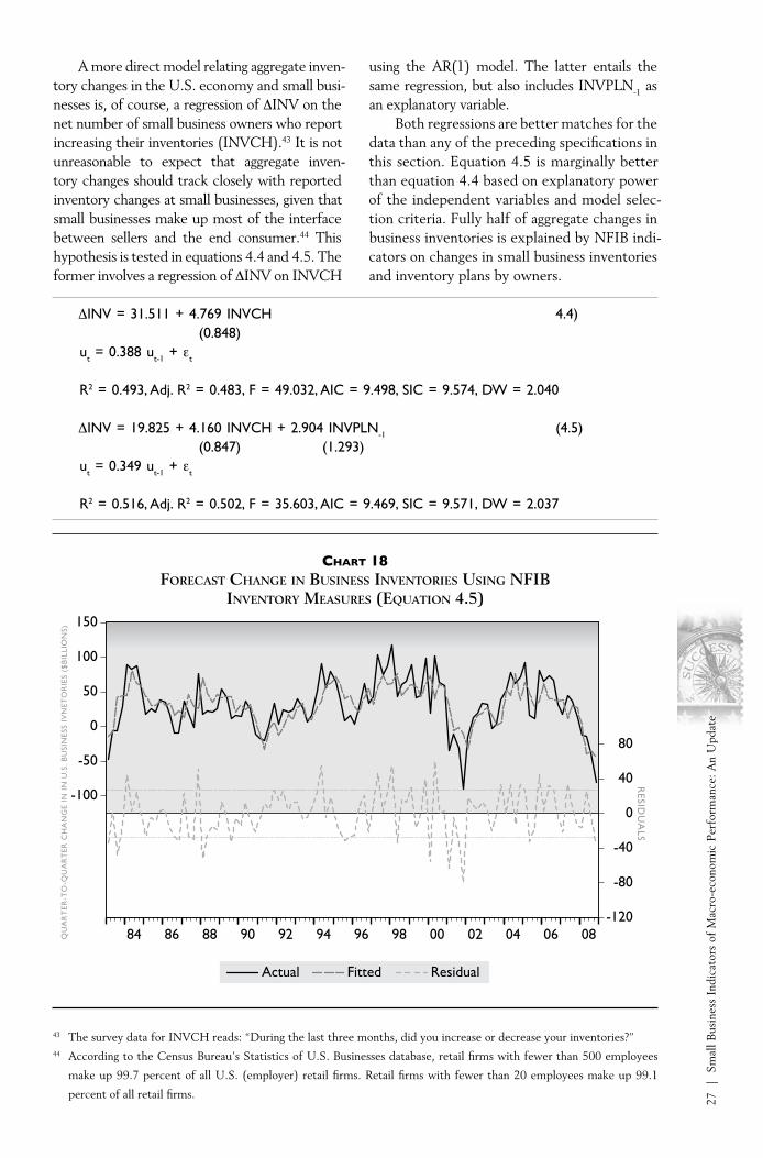
27
| S
mal
l Bus
ines
s In
dica
tors
of
Mac
ro-e
cono
mic
Per
form
ance
: An
Upd
ate
A more direct model relating aggregate inven-tory changes in the U.S. economy and small busi-nesses is, of course, a regression of ∆INV on the net number of small business owners who report increasing their inventories (INVCH).43 It is not unreasonable to expect that aggregate inven-tory changes should track closely with reported inventory changes at small businesses, given that small businesses make up most of the interface between sellers and the end consumer.44 This hypothesis is tested in equations 4.4 and 4.5. The former involves a regression of ∆INV on INVCH
using the AR(1) model. The latter entails the same regression, but also includes INVPLN-1 as an explanatory variable.
Both regressions are better matches for the data than any of the preceding specifications in this section. Equation 4.5 is marginally better than equation 4.4 based on explanatory power of the independent variables and model selec-tion criteria. Fully half of aggregate changes in business inventories is explained by NFIB indi-cators on changes in small business inventories and inventory plans by owners.
∆INV = 31.511 + 4.769 INVCH 4.4) (0.848)ut = 0.388 ut-1 + εt
R2 = 0.493, Adj. R2 = 0.483, F = 49.032, AIC = 9.498, SIC = 9.574, DW = 2.040
∆INV = 19.825 + 4.160 INVCH + 2.904 INVPLN-1 (4.5) (0.847) (1.293)ut = 0.349 ut-1 + εt
R2 = 0.516, Adj. R2 = 0.502, F = 35.603, AIC = 9.469, SIC = 9.571, DW = 2.037
Chart 18forecaSt chanGe in BuSineSS inventorieS uSinG nfiB
inventory meaSureS (equation 4.5)
43 The survey data for INVCH reads: “During the last three months, did you increase or decrease your inventories?”44 According to the Census Bureau’s Statistics of U.S. Businesses database, retail firms with fewer than 500 employees
make up 99.7 percent of all U.S. (employer) retail firms. Retail firms with fewer than 20 employees make up 99.1
percent of all retail firms.
QU
AR
TER
-TO
-QU
AR
TER
CH
AN
GE
IN I
N U
.S.
BU
SIN
ESS
IVN
ETO
RIE
S ($
BIL
LIO
NS)
RESID
UA
LS
-120
-80
-40
0
40
80
-100
-50
0
50
100
150
84 86 88 90 92 94 96 98 00 02 04 06 08
ResidualActual Fitted

28
| S
mal
l Bus
ines
s In
dica
tors
of
Mac
ro-e
cono
mic
Per
form
ance
: An
Upd
ate
The tendency to accurately predict out-of-sample directional movements in a macroeco-nomic variable but “undershoot” local maxima and minima is also found with the NFIB models of changes in inventory. An out-of-sample fore-cast using equation 4.3 (Chart 19) shows how
the NFIB models predict the large decrease in business inventories in the years following the financial crisis, but underestimated the degree of the inventory “fire sale.” The predicted changes appear to be highly sensitive to swings in the INVPLN variable.
Actual Predicted
QU
AR
TER
-TO
-QU
AR
TER
CH
AN
GE
IN U
.S.
BU
SIN
ESS
INV
ENT
OR
IES
($B
ILLI
ON
S)
-200
-160
-120
-80
-40
0
40
80
120
1975 1980 1985 1990 1995 2000 2005 2010
Chart 19out-of-SamPle forecaSt of chanGe in BuSineSS inventorieS uSinG equation 4.3

29
| S
mal
l Bus
ines
s In
dica
tors
of
Mac
ro-e
cono
mic
Per
form
ance
: An
Upd
ate
caPital exPenditureS
This section discusses the predictive ability NFIB capital expenditure mea-sures by small business owners (planned or actual) hold toward aggregate measures of capital expenditure. The NFIB measures prove to be poor predictors of changes in gross private domestic investment, but reasonably good predictors of changes in fixed capital spending.
%∆CAPX = -24.945 - 0.557 CXPAST + 1.950 CXPLAN (5.1) (0.298) (0.466)
R2 = 0.141, Adj. R2 = 0.127, F = 9.627, AIC = 8.285, SIC = 8.354, DW = 1.761
%∆PRIVFIXED = -14.001 - 0.472 CXPAST + 1.431 CXPLAN (5.2) (0.230) (0.274)ut = 0.510 ut-1 + εt
R2 = 0.453, Adj. R2 = 0.438, F = 31.687, AIC = 6.819, SIC = 6.912, DW = 1.916
%∆NONRESPRIVFIX = -25.928 - 0.165 CXPAST + 1.270 CXPLAN (5.3) (0.194) (0.258)
Although individual firms rarely make massive capital outlays, the accumulation of small outlays by six million small business employers can have a substantial impact on aggregate capital spending in the United States. The median outlay for NFIB members is $20,000 (in the prior six months), typically reported by 50 percent to 70 percent of the owners from quarter to quarter. Four percent of the owners typically report outlays in excess of $500,000 (in the prior six months).
The relationship between gross private domestic investment (%∆CAPX) and the NFIB indicators CXPAST,45 the incidence of past capital spending, and CXPLAN, the percent of owners planning capital outlays in the next three to six months, is not particu-larly strong (Equation 5.1). The two NFIB capital expenditure variables explain just 14.1 percent of changes in overall private invest-ment. Narrowing the definition of invest-ment spending improves the fit. CXPAST and CXPLAN hold substantially greater explan-
atory power toward changes in private fixed investment (%∆PRIVFIXED and %∆NONRE-SPRIVFIX) or equipment only (%∆NONRE-SEQUIP) [Equations 5.2, 5.3, and 5.4]. All equations are estimated with data beginning in 1979:Q1, the first quarter that NFIB past expenditure data are available.
The NFIB measures do best in estimating changes in total private fixed investment, explaining 45.3 percent of the quarter-to-quarter changes. CXPAST and CXPLAN also explain 35.2 percent of movements in nonres-idential equipment purchases. Of the four regressions, model selection criteria hint that equation 5.3 provides the best specification, but the high p-value for CXPAST’s coeffi-cient (0.325) suggests otherwise. The negative sign on CXPAST suggests that if owners spent money on capital expenditures in the previous period, they are likely to spend less during the current period (for example, more of the gap between desired and actual capital stock was closed in a prior period).
45 The survey question for CXPAST data reads: “During the last six months has your firm made any capital expenditures
to improve or purchase equipment, buildings, or lands?”
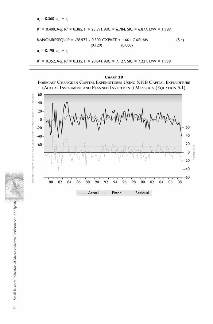
30
| S
mal
l Bus
ines
s In
dica
tors
of
Mac
ro-e
cono
mic
Per
form
ance
: An
Upd
ate
ut = 0.360 ut-1 + εt
R2 = 0.400, Adj. R2 = 0.385, F = 25.591, AIC = 6.784, SIC = 6.877, DW = 1.989
%∆NONRESEQUIP = -28.972 - 0.300 CXPAST + 1.661 CXPLAN (5.4) (0.129) (0.000)ut = 0.198 ut-1 + εt
R2 = 0.352, Adj. R2 = 0.335, F = 20.841, AIC = 7.127, SIC = 7.221, DW = 1.938
Chart 20forecaSt chanGe in caPital exPenditureS uSinG nfiB caPital exPenditure
(actual inveStment and Planned inveStment) meaSureS (equation 5.1)
QU
AR
TER
-TO
-QU
AR
TER
CH
AN
GE
IN G
RO
SS D
OM
EST
IC P
RIV
AT
E IN
VES
TM
ENT
(PE
RC
ENT
)
RESID
UA
LS
ResidualActual Fitted
-60
-40
-20
0
20
40
60
-60
-40
-20
0
20
40
60
80 82 84 86 88 90 92 94 96 98 00 02 04 06 08

31
| S
mal
l Bus
ines
s In
dica
tors
of
Mac
ro-e
cono
mic
Per
form
ance
: An
Upd
ate
Chart 21forecaSt chanGe in Private fixed inveStment uSinG nfiB caPital exPenditure
(actual inveStment and Planned inveStment) meaSureS (equation 5.2)
%∆PRIVFIXED = -19.379 + 0.736 CXPLAN (5.5) (0.209)ut = 0.501 ut-1 + εt
R2 = 0.368, Adj. R2 = 0.358, F = 39.548, AIC = 7.154, SIC = 7.217, DW = 1.972
%∆NONRESPRIVFIX = -20.821 + 0.821 CXPLAN (5.6) (0.173)ut = 0.446 ut-1 + εt
R2 = 0.380, Adj. R2 = 0.371, F = 41.699, AIC = 6.893, SIC = 6.956, DW = 2.066
Much of the explanatory power toward fixed investment in the previous equations appears to have its source in CXPLAN. Regressions of %∆PRIVFIXED and %∆NONRESPRIVFIX on
CXPLAN using an AR(1) model show that the NFIB variable individually explains more than 35 percent of changes in either investment measure (Equations 5.5 and 5.6).
QU
AR
TER
-TO
-QU
AR
TER
CH
AN
GE
IN P
RIV
AT
E FI
XED
IN
VES
TM
ENT
(PE
RC
ENT
)
RESID
UA
LS
-30
-20
-10
0
10
20
30
-60
-40
-20
0
20
40
80 82 84 86 88 90 92 94 96 98 00 02 04 06 08
ResidualActual Fitted
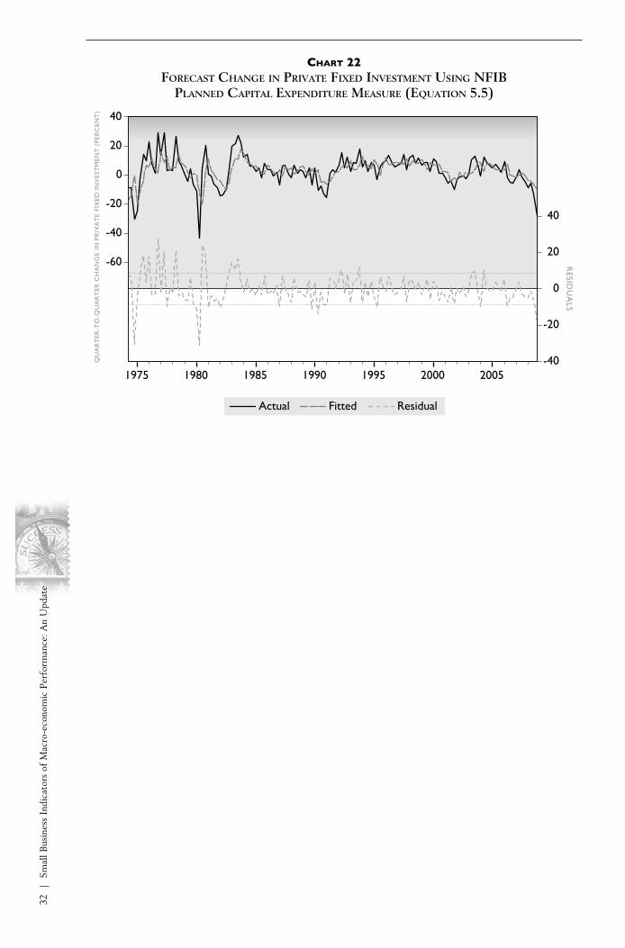
32
| S
mal
l Bus
ines
s In
dica
tors
of
Mac
ro-e
cono
mic
Per
form
ance
: An
Upd
ate
Chart 22forecaSt chanGe in Private fixed inveStment uSinG nfiB
Planned caPital exPenditure meaSure (equation 5.5)
QU
AR
TER
-TO
-QU
AR
TER
CH
AN
GE
IN P
RIV
AT
E FI
XED
IN
VES
TM
ENT
(PE
RC
ENT
)
RESID
UA
LS
-40
-20
0
20
40
-60
-40
-20
0
20
40
1975 1980 1985 1990 1995 2000 2005
ResidualActual Fitted

33
| S
mal
l Bus
ines
s In
dica
tors
of
Mac
ro-e
cono
mic
Per
form
ance
: An
Upd
ate
caPital marketS
This section highlights the strong bivariate relationship NIFB measures of small business credit tightness have with broad measures of capital mar-ket tightness, including the federal funds rate and the interest rates paid on T-bills and 10-year treasury notes.
During the formation phase, small firms are financed primarily using the savings of the entrepreneur(s) or those of his friends and rela-tives. Once the initial phases of business forma-tion have passed, owners and managers usually turn to other funding sources to finance oper-ations. Access to capital through conventional credit markets typically takes on a more impor-tant role as new businesses mature. The most important source of credit for small businesses consists of commercial banks and other deposi-tory institutions, like savings banks and thrifts. Banks serve as the primary source of funds for capital expenditures by small businesses, although credit cards have increasingly become a source for small business capital expenditure financing. Most of the bank lending done with small businesses takes the form of a traditional business loan such as a line of credit, a mort-gage loan, or an equipment loan.
Numerous factors can influence the outcome of a potential borrower’s attempt to acquire credit from a lender. Among these is federal monetary policy, which is implemented through bond market transactions conducted by the Federal Reserve Bank of New York. These transactions, also known as open market operations, have a significant impact on the federal funds rate (FEDFUNDS), the rate at which banks lend to each other overnight. Under normal circumstances, the federal funds rate subsequently influences other interest rates throughout the economy by acting as an interest rate floor for credit transactions. In the context of bank lending decisions, banks will lend to potential borrowers when the
expected return on investment for the loan exceeds the opportunity cost of leaving the loan funds with the Federal Reserve for inter-bank lending. Movements in the federal funds rate lead to movements in other interest rates in the same direction, including the interest rates offered by banks for small business loans, although since 2008 there seems to be a discon-nect as the average rate paid on twelve-month money by small business owners is stuck at 6 percent while the fed funds rate is near zero. The present inability of the average small busi-ness loan rate to fall below 6 percent may be a reflection of the risk premium lenders place on borrowers who seek capital to fund small businesses.
The NFIB survey collects data on the reported average interest rate paid by owners who borrowed using short term business loans (AVRATE). Chart 23 shows how movements in AVRATE track closely not only with move-ments in the fed funds rate, but also with other major indicators of credit market tightness like the yield on the 1-year treasury bill (TBILL) and the yield on the 10-year treasury note (TNOTE). Movements in AVRATE closely mirror those of FEDFUNDS with an average of 4.6 percentage points separating the two series starting in 1981:Q2, the first quarter data for AVRATE was collected. Table 2 presents the correlation matrix for these four time series. AVRATE is strongly correlated with all three other vari-ables. The correlation between AVRATE and FEDFUNDS (ρ = 0.9641) is almost as strong as the correlation between the federal funds rate and the T-bill yield (ρ 0.9891).

34
| S
mal
l Bus
ines
s In
dica
tors
of
Mac
ro-e
cono
mic
Per
form
ance
: An
Upd
ate
Chart 23nfiB averaGe intereSt rate for Small BuSineSSeS comPared
with common intereSt rateS, 1974:q4 to 2011:q3
table 2 correlation matrix of nfiB averaGe rate and common intereSt rateS
AVRATE FEDFUNDS TBILL TNOTE
AVRATE 1.0000 FEDFUNDS 0.9641 1.0000 TBILL 0.9636 0.9891 1.0000 TNOTE 0.9378 0.9178 0.9508 1.0000
INT
ERES
T R
AT
E (P
ERC
ENT
)
AV RATE FED FUNDS
T BILL T NOTE
0
4
8
12
16
20
1975 1980 1985 1990 1995 2000 2005 2010
The strong correlation between AVRATE and FEDFUNDS shows the influence federal monetary policy can have on small business lending. Given this strong relationship, it stands to reason that the federal funds rate and other interest rates which move in tandem might prove to be good predictors of measures of small business credit tightness. Two explicit survey measures of credit tightness in the small business lending market contained in the NFIB
survey are the net percent of owners reporting a harder time obtaining financing compared to three months ago (CREDHARD)46 and the reported relative interest rate paid by regular borrowers (at least once every three months) for business loans compared to three months ago (RATEPD).47 Higher levels of both vari-ables indicate tighter credit markets for small businesses.
46 The survey question for CREDHARD data reads: “If you borrow money regularly (at least once every 3 months) as part
of your business activity, how does the rate of interest payable on your most recent loan compare with that paid three
months ago?”47 The survey question for RATEPD data reads: “Are these loans easier or harder to get than they were three months ago?”
RATEPD data include only those respondents who indicated they were regular borrowers in the survey question for
CREDHARD.

35
| S
mal
l Bus
ines
s In
dica
tors
of
Mac
ro-e
cono
mic
Per
form
ance
: An
Upd
ate
Equations 6.1, 6.2, and 6.3 show the results of regressions of RATEPD on FEDFUNDS, TBILL, and TNOTE, respectively, using the first-order autoregressive model. The federal funds rate, 1-year T-bill yield, and 10-year treasury note yield are all strong predic-tors of changes in the interest rate paid by small business owners on short-term business loans. The reader here will note that unlike earlier regressions, the government data vari-able is on the right-hand side of each of these equations, reflecting the understanding that in many models, monetary policy shocks (interest rate decisions made by the Federal
Reserve) are assumed to be exogenous. The R-squares of all three regressions exceed 0.59, with FEDFUNDS providing slightly more explanatory power than TBILL or TNOTE. Positive movements FEDFUNDS, TBILL, or TNOTE indicate monetary policy tight-ening which incentivizes lenders throughout the banking system to tighten lending. This process is reflected in the borrowing experi-ences of regularly-borrowing small business owners who report higher relative interest rates in the current period (conveyed through positive regression slope coefficients in these three equations).
RATEPD = -22.947 + 4.456 FEDFUNDS (6.1) (0.787)ut = 0.823 ut-1 + εt
R2 = 0.651, Adj. R2 = 0.646, F = 127.576, AIC = 7.572, SIC = 7.635, DW = 2.267
RATEPD = -18.732 + 3.722 TBILL (6.2) (0.886)ut = 0.771 ut-1 + εt
R2 = 0.622, Adj. R2 = 0.616, F = 112.589, AIC = 7.652, SIC = 7.715, DW = 2.251
RATEPD = -20.893 + 3.457 TNOTE (6.3) (1.301)ut = 0.789 ut-1 + εt
R2 = 0.592, Adj. R2 = 0.586, F = 99.644, AIC = 7.726, SIC = 7.789, DW = 2.159

36
| S
mal
l Bus
ines
s In
dica
tors
of
Mac
ro-e
cono
mic
Per
form
ance
: An
Upd
ate
Chart 24forecaSt relative rate Paid By Small BuSineSS ownerS
uSinG federal fundS rate (equation 6.1)
As tools for generating out-of-sample forecasts of relative interest rates paid, the above three regressions all do a fairly good job predicting directional movements in RATEPD, although all three tend to underestimate the
magnitude of the variable itself, thereby under-shooting local highs in the series. Chart 25 shows the out-of-sample forecast of RATEPD estimated using equation 6.1.
Chart 25out-of-SamPle forecaSt of relative rate Paid uSinG equation 6.1
INT
ERST
RA
TE
(PER
CEN
T)
RESID
UA
LS
-60
-40
-20
0
20
-40
-20
0
20
40
60
1975 1980 1985 1990 1995 2000 2005
ResidualActual Fitted
REL
AT
IVE
INT
ERST
RA
TE
(PER
CEN
T)
Actual Predicted
-30
-20
-10
0
10
20
30
40
50
1975 1980 1985 1990 1995 2000 2005 2010

37
| S
mal
l Bus
ines
s In
dica
tors
of
Mac
ro-e
cono
mic
Per
form
ance
: An
Upd
ate
Higher interest rates and tighter lending standards should be reflected in a higher percentage of owners who report credit harder to obtain. Regressions of CREDHARD on FEDFUNDS, TBILL, and TNOTE, respec-tively, using the first-order autoregressive model, provide evidence of this relationship (Equations 6.4, 6.5, and 6.6). Positive slope
coefficients in all three equations suggest that small business owners are sensitive to mone-tary tightening and find credit harder to obtain when interest rates rise. Although the R-squares for these three regressions are lower than those in equations 6.1, 6.2, and 6.3, they are still quite strong given the presence of just one regressor in each of the equations.
CREDHARD = 1.822 + 0.639 FEDFUNDS (6.4) (0.142)ut = 0.572 ut-1 + εt
R2 = 0.508, Adj. R2 = 0.501, F = 70.682, AIC = 4.941, SIC = 5.004, DW = 2.251
CREDHARD = 2.924 + 0.465 TBILL (6.5) (0.166)ut = 0.578 ut-1 + εt
R2 = 0.464, Adj. R2 = 0.456, F = 59.295, AIC = 5.026, SIC = 5.089, DW = 2.278
CREDHARD = 2.563 + 0.447 TNOTE (6.6) (0.222)ut = 0.609 ut-1 + εt
R2 = 0.454, Adj. R2 = 0.446, F = 56.877, AIC = 5.045, SIC = 5.108, DW = 2.300
Chart 26forecaSt net Percent of Small BuSineSS ownerS who find credit
harder to Get uSinG federal fundS rate (equation 6.4)
NET
PER
CEN
T O
F O
WN
ERS
(PER
CEN
T)
RESID
UA
LS
0
-20
-10
10
20
-10
0
10
20
30
1975 1980 1985 1990 1995 2000 2005
ResidualActual Fitted

38
| S
mal
l Bus
ines
s In
dica
tors
of
Mac
ro-e
cono
mic
Per
form
ance
: An
Upd
ate
other indicatorS
This section discusses the relative performance of the NFIB Optimism In-dex as a predictor of changes in Gross Domestic Product. The Optimism Index performs better than two widely-followed measures of consumer sen-timent, the Conference Board’s Consumer Confidence Index and the Uni-versity of Michigan’s Index of Consumer Sentiment. The Optimism Index also performs favorably compared to the Institute of Supply Management’s Purchasing Managers Index.
Numerous other survey indicators are used by analysts to track and anticipate changes in economic activity. Many of these, like the NFIB survey, reflect the sentiments and experi-ences from the firm side of the economy. Other surveys capture the views of consumers, who through their collective spending on goods and services produced in the United States, account for 70 percent of gross domestic product. The overwhelming importance of consumption to overall production in the economy suggests that these measures of consumer sentiment should act as good predictors of GDP.
Two popular indices of consumer senti-ment are the Conference Board’s Consumer Confidence Index (CCI) and the University of Michigan’s Index of Consumer Sentiment (UMCSENT). The CCI is a monthly index produced using data from the Conference Board’s Consumer Confidence Survey, which is based on the responses of 5,000 house-holds. The Conference Board’s survey focuses on gauging household reaction to labor market conditions. The quarterly CCI series used here begins in 1975:Q3 and is nearly as old as the NFIB Optimism Index. The Michigan index is
produced using data from the monthly Survey of Consumer Sentiment, a survey of 500 indi-viduals which focuses on financial and income situations. The Michigan series is older than the other two time series, beginning in 1946, although the time series data used in this anal-ysis begins in 1978:Q1. All three series adopt an index reference value of 100.
Both the Conference Board index and the Michigan index are considerably more vola-tile than the NFIB Optimism Index (Chart 26), reflecting methodological differences in the indices’ constructions and disparate target populations. Differences in volatility do not indicate an absence of correlation, however, and INDEX and UMCSENT follow the same broad patterns over time (ρ = 0.776). Move-ments in INDEX and CCI are considerably less related, and the two variables possess a corre-lation coefficient of just 0.470. A complete correlation matrix among these three variables and the quarter-to-quarter percentage change in real GDP is given in Table 3. Of the three sentiment indices, the NFIB Optimism Index is the most highly correlated with changes in real GDP over time (ρ = 0.630).

39
| S
mal
l Bus
ines
s In
dica
tors
of
Mac
ro-e
cono
mic
Per
form
ance
: An
Upd
ate
Regressions of %∆RGDP on each of the three indices indicate that INDEX is the supe-rior predictor of changes in real GDP (Equa-tions 7.1, 7.2, and 7.3). The AIC and SIC measures for equation 7.1 are both lower than
their counterparts for the other two equa-tions. Additionally, INDEX explains 38.3 percent of movements in real GDP, compared to 13.5 percent for CCI and 24.2 percent for UMCSENT.
%∆RGDP = -46.208 + 0.495 INDEX (7.1) (0.054)
R2 = 0.383, Adj. R2 = 0.378, F = 83.900, AIC = 4.784, SIC = 4.827, DW = 1.805
%∆RGDP = -0.129 + 0.032 CCI (7.2) (0.027)
ut = 0.274 ut-1 + εt
Chart 27nfiB oPtimiSm index and other Sentiment indiceS
comPared to chanGeS in real GdP
table 3correlation matrix of nfiB oPtimiSm index verSuS other
Sentiment indiceS and chanGe in real GdP INDEX CCI UMCSENT %∆RGDP
INDEX 1.000 CCI 0.470 1.000 UMCSENT 0.776 0.533 1.000 %∆RGDP 0.630 0.293 0.501 1.000
QU
AR
TER
-TO
-QU
AR
TER
CH
AN
GE
IN R
EAL
GD
P (P
ERC
ENT
)
IND
EX V
ALU
E
0
20
40
60
80
100
120
140
160
-15
-10
-5
0
5
10
15
20
25
1975 1980 1985 1990 1995 2000 2005 2010
INDEX CCI
UMCSENT PCHGRGDP

40
| S
mal
l Bus
ines
s In
dica
tors
of
Mac
ro-e
cono
mic
Per
form
ance
: An
Upd
ate
R2 = 0.135, Adj. R2 = 0.122, F = 10.133, AIC = 5.103, SIC = 5.168, DW = 1.960
%∆RGDP = -8.202 + 0.126 UMCSENT (7.3) (0.000)
ut = 0.177 ut-1 + εt
R2 = 0.242, Adj. R2 = 0.229, F = 19.107, AIC = 4.978, SIC = 5.046, DW = 1.775
INDEX also compares favorably with a popular measure of economic performance in the manufacturing industry. The Institute for Supply Management’s Purchasing Managers Index for the manufacturing sector (ISM) reflects the sentiments of purchasing agents responsible for procuring the supplies neces-sary for their respective manufacturing firms to make products. The ISM is highly sensitive to business trends in the broader economy and is known to be a useful measure for gauging turning points in the business cycle. An index value above 50 indicates that activity in the manufacturing sector is increasing; a value below 50 indicates that it is decreasing.
The manufacturing sector is sometimes viewed as a proxy for large firms in general. The data do not support this view. According to data from the Census Bureau’s Statis-
tics of U.S. Businesses data set, large firms (those with 500 or more employees) made up just 1.4 percent of all manufacturing firms in 2009, a small fraction. Conversely, manufac-turing firms made up 21 percent of all large firms, a sizeable percentage, but nowhere near a majority. These data suggest that using ISM as a proxy for the large business sector and, in doing so, measuring its performance relative to INDEX as a means of making a large-versus-small business performance comparison is a questionable practice.
In a regression of %∆RGDP on ISM over the time period 1973:Q4 to 2008:Q4, the manu-facturer’s index explains 36.2 percent of move-ments in real GDP (Equation 7.4). This result is almost as good as INDEX’s performance in equation 7.1, where INDEX explained 38.3 percent of movements in real GDP.
%∆RGDP = -14.275 + 0.330 ISM (7.3) (0.000)
R2 = 0.362, Adj. R2 = 0.357, F = 78.206, AIC = 4.853, SIC = 4.895, DW = 1.694

41
| S
mal
l Bus
ines
s In
dica
tors
of
Mac
ro-e
cono
mic
Per
form
ance
: An
Upd
ate
concludinG oBServationS
The small business sector produces almost one-half of the private sector GDP, accounts for roughly half of the private sector labor force, and two-thirds of the net new jobs created. Collectively, the actions of small busi-ness owners have a major impact on the U.S. economy. The economic indicators pioneered by NFIB and described herein have been shown to have strong empirical relationships to important economic measures like GDP growth, unemployment, inflation, business inventories, and capital expenditures. The NFIB measures appear to do best predicting future movements in inflationary and labor market indicators. When serial correlation is accounted for and addressed in regression analysis, the R-squared values of regressions of inflationary indicators on NFIB measures regu-larly exceed 0.60. R-squared values of regres-sions of changes in private employment or the
unemployment rate on NFIB measures some-times exceed 0.70.
Compared with other major indicators of consumer sentiment, the relative perfor-mance of the headline NFIB Optimism Index as a predictor of changes in real GDP is shown to be superior to both the Conference Board’s Consumer Confidence Index and the Univer-sity of Michigan’s Index of Consumer Senti-ment. The NFIB Optimism Index is also shown to perform favorably when compared to the ISM Purchasing Managers Index, an indicator sometimes thought to represent economic activity in “larger” firms. The strong performance of NFIB measures as predictors of headline macroeconomic indicators should encourage their increased use by forecasters, policymakers, and other analysts for fore-casting, policymaking, and comprehending how one vital half of the economy performs.

aPPendix a: Small BuSineSS economic Survey
42
| S
mal
l Bus
ines
s In
dica
tors
of
Mac
ro-e
cono
mic
Per
form
ance
: An
Upd
ate

43
| S
mal
l Bus
ines
s In
dica
tors
of
Mac
ro-e
cono
mic
Per
form
ance
: An
Upd
ate

44
| S
mal
l Bus
ines
s In
dica
tors
of
Mac
ro-e
cono
mic
Per
form
ance
: An
Upd
ate

45
| S
mal
l Bus
ines
s In
dica
tors
of
Mac
ro-e
cono
mic
Per
form
ance
: An
Upd
ate

46
| S
mal
l Bus
ines
s In
dica
tors
of
Mac
ro-e
cono
mic
Per
form
ance
: An
Upd
ate
aPPendix B. noteS reGardinG model SPecification and Selection
When performing regression analysis, one of the questions a researcher must concern himself with is model specification. This endeavor includes selecting the dependent variable, independent variable(s), and func-tional form of the equation, and deciding whether these choices collectively provide for the most “appropriate” model specifica-tion. Broadly speaking, deciding the “appro-priateness” of a model specification occurs on two levels. First, economic theory and intuition can be relied upon when deciding whether certain independent variables should be included in the model to “explain” move-ments in the dependent variable regardless of the statistical significance of the regres-sion coefficients or the impact their inclusion has on measures of goodness-of-fit or model selection criteria. For this reason, readers will sometimes encounter regressions in which explanatory variables whose t-statistics and p-values are not significant at a chosen level of significance have nonetheless been included in the final model specification.
The second approach is to rely (more) strictly upon the regression results to help inform what explanatory variables should be included or omitted in the final specification. This involves not only checking the statistical significance of individual t-statistics and p-values, but also examining model selection criteria that
statisticians and econometricians have devel-oped which serve as a useful way of discerning and selecting among alternative model specifi-cations. These selection criteria generally seek to minimize some function of the mean squared error (MSE), defined as the sum of the resid-uals from a regression divided by the number of observations: MSE = (∑et
2 / T). This mono-graph refers to two such model selection criteria throughout. The first is the Akaike Information Criterion (AIC), defined as AIC = e(2p/T) * MSE, where p is the number of parameters to be esti-mated in the regression and T is the number of observations. The second model selection crite-rion is the Schwarz Information Criterion (SIC), defined as SIC = T(p/T) * MSE.
An interesting feature of the AIC and SIC measures is that neither of them are associ-ated with a statistical distribution. This lack of an underlying distribution naturally makes it impossible to mathematically prove the effi-ciency or robustness of these criteria. In lieu of proofs, monte carlo simulations have been used to confirm the robustness of these measures. Lack of an underlying distribution also makes it impossible to use these measures in tests of statistical significance. Instead, analysts who use the AIC or SIC measures to select a “best” model specification follow the rule of thumb of selecting the model with the lowest AIC or SIC measure.

47
| S
mal
l Bus
ines
s In
dica
tors
of
Mac
ro-e
cono
mic
Per
form
ance
: An
Upd
ate
aPPendix c. noteS reGardinG time SerieS analySiS
All of the data used in this analysis is time series data, meaning that a system of temporal ordering is associated with the data. This is the principal difference distinguishing time series data from cross-sectional data and introduces certain complications in data analysis. Fore-most among these complications is the risk of finding a relationship between two or more time series variables simply because all of them trend over time. Failure to account for time trends may lead an observer to falsely conclude that changes in a particular variable are causing the changes in the other variables(s). In many cases, there are usually one or more variables omitted from the analysis which are driving the trends observed among the included variables. This danger is referred to in the econometrics literature as the spurious regression problem, for which certain analytical techniques (other than including the omitted factors) have been developed in order to mitigate the risk of this phenomenon’s occurrence. An additional complication found in cases when the depen-dent variable is trending is artificially high R2 and adjusted R2 values.
One approach used to address the spurious regression problem is to include a time trend variable(s) in the regression equation, thereby explicitly recognizing that changes in the dependent variable may be caused for reasons essentially unrelated to changes in the indepen-dent variables. Failure to include a time trend variable(s) in the absence of other econometric adjustments will typically yield biased regres-sion coefficients of the independent variables. Time trends observed for a particular economic time series need not be linear, although this is frequently the case. An exponential trend, for example, is a better tool when attempting to approximate a time series exhibiting a more-or-less constant growth rate over time. While including a time trend variable(s) is a straight-forward method for reducing the likelihood of obtaining biased estimators through regres-sion analysis, it is nonetheless at least some-what unsatisfactory at an intuitive level due to the knowledge that the econometric model is
incomplete (factors have been omitted from the regression equation). Ultimately, whether or not this approach is sufficient depends on the analysis at hand. Including time trend variable(s) may be satisfactory if the emphasis lies in forecasting, for instance, but it may not be satisfactory if the desire is to construct a theoretically sound and “fully explained” model.
Another approach that can be used to address the spurious regression problem in the case of a variable(s) trending over time is differencing prior to regressing: subtracting the value of the variable during a given time period from its value during the period immediately preceding and then using the “differenced” time series in lieu of the original series when performing regression analysis. In the case of linear time trends, taking one “difference” is frequently sufficient to avoid the spurious regression problem, although the interpreta-tion of regression results is now different.
Differencing in the context of time series regressions is especially common in large sample analysis when classical linear model assump-tions are not satisfied. In such cases, the tradi-tional statistical measures calculated during regression analysis (t-statistics, F-statistics, etc.) will not follow the assumed distribution. That is, the t-statistic as calculated using the conventional equation for the t-distribution will not follow the t-distribution; the F-statistic as calculated using the conventional equation for the F-statistic will not follow the F-distribution; and so on. When this occurs, meaningful results from regression analysis require key conditions of asymptotic theory to be fulfilled, including, of course, the expectation that the sample size is sufficiently large. If the conditions are met, then the asymptotic (large sample) properties of esti-mators and test statistics are not only known, but also approximate the relevant distributions. The econometrician is then able to perform standard tests of statistical significance.
In time series analysis, the principal asymp-totic condition differencing attempts to achieve is weak dependence, a concept which is best addressed in the context of stationary time
48
| S
mal
l Bus
ines
s In
dica
tors
of
Mac
ro-e
cono
mic
Per
form
ance
: An
Upd
ate
series. Generally speaking, a stationary time series process is one whose probability distribu-tions are stable over time. A stationary time series {xt: t = 1, 2, …} is said to be weakly dependent if for any value of t, xt and xt+h are “almost inde-pendent” as h → ∞. By imposing a limit on how strongly related two different values in a time series can be, weak dependence, along with the stationarity requirement, ensures that the most well-known central limit theorem for time series data is satisfied. Weak dependence is impor-tant for time series regression analysis because it essentially replaces the random sampling assumption required in large sample cross-section analysis. (Random sampling is required for the law of large numbers and central limit theorem to hold in cross-section analysis.)
Weakly dependent processes are said to be integrated of order zero, denoted I(0). Processes which are not weakly dependent are integrated to a higher order. Much could be said about such processes, but we will limit the discussion here by simply mentioning that such processes are denoted by I(x), where x is the integration order of the process. A process that is integrated of order one is referred to as a unit root process. For the practitioner’s purposes, all that need be known is that the integration order is the number of differences that must be taken for a process to (likely) be made weakly dependent. Readers interested in a more exten-sive treatment of the concept of integration may wish to refer to Wooldridge (2009).48
It should be remarked briefly that the notions of trending, stationarity, and weak dependency are separate and distinct. Trending series are capable of being both stationary or nonstationary, as well as weakly dependent or not. Simply because a series is trending does not mean that it is nonstationary. Likewise, simply because a series is stationary does not mean that it is weakly dependent. A weakly dependent series that is stationary about its time trend is often referred to as a trend-stationary process and can be used in regres-sion analysis provided appropriate time trends are included in the model.
A common test for weak dependence that accounts for complicated dynamics in the model is the Augmented Dickey-Fuller (ADF) test, which tests for the presence of a unit root. In such tests, the null hypothesis is that a unit
root exists. Failure to reject the null hypothesis is not evidence that a unit root exists; it simply means that one cannot rule out the presence of a unit root. In practice, when differencing to obtain a weakly dependent series, an analyst will typically perform an ADF test and check to see if the null hypothesis is rejected or not. If not, then the series is differenced once and another ADF test is performed on the differ-enced series. This process is repeated until the null hypothesis of the ADF test is rejected.
The desire to generate time series that are not weakly dependent into ones that are explains why one frequently observes differenced series among independent and dependent variables in time series regressions. However, strict applica-tion of the ADF test is not especially common outside certain forecasting projects since doing so can limit the ability of the analyst to inter-pret the results in an economically-meaningful way. Regressions may therefore include a set of differenced time series which represent a combination of weakly dependent and not weakly dependent series. The need for regres-sion results to be economically meaningful also motivates the inclusion into regression models of time series variables which are expressed not in terms of period-to-period differences (which may be weakly dependent), but rather vari-ables expressed as period-to-period percentage changes of the original series. For example, time series data of an economic index are better expressed in percentage change terms instead of period-to-period differences.
Differencing has the potential added benefit of correcting the problem of serial correlation in the error terms. Serial corre-lation, also called autocorrelation, in the error terms is a common problem in time series anal-ysis and refers to the phenomenon when error terms (conditional upon the independent vari-ables) in two different time periods are corre-lated with one another. Failure to correct for serial correlation will raise doubts about the reliability of time series regression results since its presence means that ordinary least squares (OLS) no longer produces best, linear, unbi-ased estimators, as the variance estimators for OLS coefficients are now biased. More impor-tantly, traditional OLS standard errors and test statistics (t, F, LM) are no longer valid in the presence of serial correlation.
48 Wooldridge, Jeffrey M., Introductory Econometrics: A Modern Approach, 4th edition, 2009.

49
| S
mal
l Bus
ines
s In
dica
tors
of
Mac
ro-e
cono
mic
Per
form
ance
: An
Upd
ate
aPPendix d. auGmented dickey-fuller teSt reSultS
The Augmented Dickey-Fuller (ADF) test is a common test for weak dependence in a time series. The null hypothesis of an ADF test is that a unit root exists. If the test results fail to reject the null hypothesis, an analyst concerned about potential complications due to possible weak dependence among the data may elect to take differences of the time series tested until the null hypothesis of subsequent ADF tests on differenced series is rejected. Such an approach follows guidelines set forth in the Box-Jenkins methodology for time series analysis.
Table 4 below gives the results of ADF tests on all variables, both dependent and independent, contained in regressions in the preceding sections. Tests were run for each time series beginning with the earliest data point available through 2011:Q3. Nearly all variables presented in differenced (∆) form or quarterly change (%∆) form reject the ADF test null hypothesis at the five percent signifi-cance level. Those variables that do not reject the null hypothesis at the five percent signif-
icance level reject it at the ten percent level. For those variables presented in their original form (with no transformations applied), many reject the null at the five percent significance level, but many also do not, nor do they reject the null at the ten percent significance level. In fact, the p-values and t-statistics for some would suggest at least one level of differencing be applied, were the Box-Jenkins methodology followed strictly. However, transforming these variables and including the resulting data series into the appropriate regression equations above would in many cases make the economic interpretation of the equations more difficult. In deference to simplicity and economic intu-ition, these variables were left untransformed even when ADF test results suggested that differencing might prove beneficial (higher R2
values, lower AIC/SIC values).More information regarding the ADF test
and potential complications resulting from weak dependence among the data may be found in the appendix on time series analysis.

50
| S
mal
l Bus
ines
s In
dica
tors
of
Mac
ro-e
cono
mic
Per
form
ance
: An
Upd
ate
table 4auGmented dickey-fuller teSt reSultS
Test critical values Variable Name t-statistic 1% level 5% level 10% level p-value
%∆CAPX -8.7327 -4.0208 -3.4403 -3.1446 0.0000%∆CPI -3.6143 -4.0217 -3.4407 -3.1448 0.0320%∆CPICORE -3.4015 -4.0217 -3.4407 -3.1448 0.0551%∆ECI -4.7808 -4.1985 -3.5236 -3.1929 0.0021%∆FSAL -6.0577 -4.0213 -3.4405 -3.1447 0.0000%∆FSALPRIV -6.9904 -4.0208 -3.4403 -3.1446 0.0000%∆GDPDFL -3.2737 -4.0213 -3.4405 -3.1447 0.0747%∆NONRESEQUIP -4.9204 -4.0213 -3.4405 -3.1447 0.0005%∆NONRESPRIVFIX -6.1182 -4.0208 -3.4403 -3.1446 0.0000%∆PCE -3.7450 -4.0217 -3.4407 -3.1448 0.0224%∆PRIVFIXED -6.2897 -4.0204 -3.4401 -3.1445 0.0000%∆RGDP -8.7464 -4.0208 -3.4403 -3.1446 0.0000∆INV -13.3886 -4.0208 -3.4403 -3.1446 0.0000∆PRIVEMPL -4.4415 -4.0208 -3.4403 -3.1446 0.0026∆u -5.3653 -4.0217 -3.4407 -3.1148 0.0001 CCI -2.6848 -4.0290 -3.4442 -3.1469 0.2447CREDHARD -3.4255 -4.0204 -3.4401 -3.1445 0.0518CXPAST -1.7664 -4.0302 -3.4448 -3.1472 0.7154CXPLAN -3.1123 -4.0217 -3.4407 -3.1448 0.1073EBCD -4.0065 -4.0200 -3.4399 -3.1443 0.0104EMPCH -3.7442 -4.0259 -3.4427 -3.1460 0.0226ESAL -4.9453 -4.0200 -3.4399 -3.1443 0.0004ESAL-1 -5.0022 -4.0204 -3.4401 -3.1445 0.0003FEDFUNDS -4.2851 -4.0226 -3.4411 -3.1451 0.0044GTEX -3.0442 -4.0200 -3.4399 -3.1443 0.1239INDEX -3.9361 -4.0217 -3.4407 -3.1448 0.0129INVCH -3.0176 -4.0398 -3.4494 -3.1499 0.1320INVPLN-1 -3.4792 -4.0213 -3.4405 -3.1447 0.0454INVSAT-1 -6.0915 -4.0204 -3.4401 -3.1445 0.0000ISM -6.2403 -4.0200 -3.4399 -3.1443 0.0000NJOBOP -2.4084 -4.0200 -3.4399 -3.1443 0.3737PASTP -3.4925 -4.0217 -3.4407 -3.1448 0.0439PASTP>5 -3.1825 -4.0204 -3.4401 -3.1445 0.0919PHIGHER -2.5229 -4.0235 -3.4416 -3.1453 0.3168PLANP -3.2909 -4.0200 -3.4399 -3.1443 0.0717PLANP-1 -3.1762 -4.0204 -3.4401 -3.1445 0.0932PLANP>5 -3.0432 -4.0221 -3.4409 -3.1450 0.1243PLANWAGE-1 -1.9851 -4.0461 -3.4524 -3.1517 0.6025PLOWER -2.8015 -4.0217 -3.4407 -3.1448 0.1992RATEPD -4.7067 -4.0200 -3.4399 -3.1443 0.0010SAL -3.5923 -4.0217 -3.4407 -3.1448 0.0339TBILL -3.0309 -4.0217 -3.4407 -3.1448 0.1275TNOTE -2.9853 -4.0208 -3.4403 -3.1446 0.1399UMCSENT -2.1204 -4.0290 -3.4442 -3.1469 0.5294XLFCH -2.6884 -4.0204 -3.4401 -3.1445 0.2430
51
| S
mal
l Bus
ines
s In
dica
tors
of
Mac
ro-e
cono
mic
Per
form
ance
: An
Upd
ate
aPPendix e. GranGer cauSality teSt reSultS and forecaSt analySiS
Economic indicators are valuable for reasons other than the information they convey regarding certain facets of the economy. For many observers, the primary value of economic indicators lies in their ability to predict and
“lead” other indicators released at a later date. Knowledge that movements in one indicator can (to a certain degree) accurately predict the behavior of subsequently released indicators is a valuable commodity in the realm of finance.
When considering the value of NFIB vari-ables for forecasting future instances of govern-ment economic time series, two methods of analysis naturally present themselves. The first
approach involves measuring the information content that past instances of NFIB variables have on current instances of government vari-ables. A common technique implementing this approach is the Granger causality test, in which the current instance of the dependent vari-able, yt, is regressed on lagged values of itself as well as lagged values of some other variable x. y is said to be “Granger-caused” by x if the coefficients on the lagged x-values are statis-tically significant, signifying that the informa-tion content of the x time series helps in the prediction of y. Formally, the regression equa-tion is stated as:
yt = α0 + α1 * yt - 1 + … + α
l * y
t – l + β1 * xt
- 1 + … + βl * x
t - l + ε
t,
where l signifies the number of lagged periods. It should be emphasized that although test results may indicate that a certain variable x “Granger causes” another variable y, this does not imply that x causes y in the normal sense of the word. Granger causality is simply a measure of precedence and information content. Granger causality tests can no more determine “true” causality than can any other econometric technique.
Table 5 gives results of Granger causality tests performed for many of the NFIB and government economic variables contained in the above regression equations. An initial test was performed with l equal to 2, the default setting for the econometric software program used. Because the theory behind Granger causality stresses the importance of past information, as a general principal, it is better to use more rather than fewer lags in a Granger causality test. To this end, as a check
for robustness, a second test was performed with l equal to 4.
The null hypothesis in each of these tests is that the variable x does not Granger-cause the variable y. A low p-value indicates that the null hypothesis is rejected for a partic-ular level of significance. The threshold for inclusion into the table is rejection of the null hypothesis at the ten percent signif-icance level for l equal to 2. In almost all cases, the addition of two additional lagged instances of x and y in the regression equa-tion raised the p-values associated with the Granger causality tests, with a few notable exceptions.48 Major economic indicators like real GDP, the unemployment rate, and key inflation indices, among others, are shown to be “Granger caused” by NFIB variables. Of particular interest is the valuable informa-tion content contained in PASTP and PLANP toward a variety of different price indices.
48 (y, x) = {(∆PRIVEMPL, XLFCH), (∆PRIVEMPL, NJOBOP), (%∆PCE, PASTP), (%∆PCE, PLANP), (%∆PCECORE,
PLANP), (%∆GDPDFL, PLANP), (%∆INV, INVCH), (%∆CAPX, CXPAST)}.

52
| S
mal
l Bus
ines
s In
dica
tors
of
Mac
ro-e
cono
mic
Per
form
ance
: An
Upd
ate
table 5GranGer cauSality teSt reSultS
y x p-value l = 2 l = 4
%∆RGDP INDEX 0.0005 0.0035%∆RGDP ESAL 0.0005 0.0005%∆RGDP EBCD 0.0855 0.1838%∆RGDP GTEX 0.0021 0.0023%∆FSAL SAL 0.0213 0.1438%∆FSAL ESAL 0.0031 0.0050%∆FSAL NEARN 0.0510 0.1689%∆FSALPRIV ESAL 0.0849 0.0098∆u EMPCH 0.0586 0.3845∆u XLFCH 0.0781 0.1662∆PRIVEMPL EMPCH 3.E-14 1.E-12∆PRIVEMPL XLFCH 0.0008 2.E-11∆PRIVEMPL NJOBOP 0.0040 5.E-13%∆ECIWAGSAL PASTWAGE 0.0168 0.0638%∆ECIWAGSAL PLANWAGE 0.0026 0.0092%∆CPI PASTP 0.0007 0.0014%∆CPI PLANP 0.0105 0.0531%∆CPICORE PASTP 0.0002 0.0038%∆CPICORE PLANP 0.0005 0.0016%∆PCE PASTP 0.0059 0.0003%∆PCE PLANP 0.0737 0.0291%∆PCECORE PASTP 0.0231 0.0387%∆PCECORE PLANP 0.0441 0.0140%∆GDPDFL PASTP 0.0002 0.0021%∆GDPDFL PLANP 0.0056 0.0049%∆INV INVCH 0.0514 0.0390%∆INV INVSAT 0.0182 0.0852%∆INV INVPLN 3.E-05 8.E-05%∆CAPX CXPAST 0.0848 0.0384
The second approach of analyzing the value NFIB variables hold toward forecasting future values of other economic indicators entails employing previously estimated (using
“in sample” data) regression models, where the dependent variables are government statistics of interest, to forecast the next n number of values for the dependent variable, and then comparing the “out of sample” forecast values with the actual data. The most interesting statistics computed during such “forecast anal-ysis” are functions of the forecast error, the difference between the predicted and actual values. A good forecasting model will tend to minimize these errors.
At its core, forecasting accuracy depends upon how reliably past trends act as predic-tors of what is to come. The forecasting accu-
racy of a particular model estimated using past data can be very good for estimating “in sample” values which previously occurred, but may fare poorly when projecting “out of sample” future values, especially when some event(s) constituting an exogenous shock or a structural break occurs, changing the trajec-tory and behavior of economic trends tempo-rarily or even permanently. The financial crisis, housing crash, and ensuing Great Reces-sion beginning in 2007/8 constitute one such shock. Unemployment rose to levels not seen in decades, GDP contracted at some of the most rapid rates on record, and small busi-ness owners cut wages and prices and reduced inventory at the quickest pace in the history of the NFIB series. Such irregular, record-setting occurrences will obviously have a deleterious

53
| S
mal
l Bus
ines
s In
dica
tors
of
Mac
ro-e
cono
mic
Per
form
ance
: An
Upd
ate
impact on out-of-sample forecast analysis using the above models, considering that the models were estimated using data through the end of 2008.
Despite these considerations, several of the regression models discussed above proved
to be good predictors when used to forecast out-of-sample estimates (2009:Q1 through 2011:Q4). In particular, the inflation regres-sions along with models of labor market measures proved to be good predictors of out-of-sample (actual) values.

1201 “F” Street, NWSuite 200Washington, DC 20004 nfib.com