Ryan Jarret - Vanderbilt University

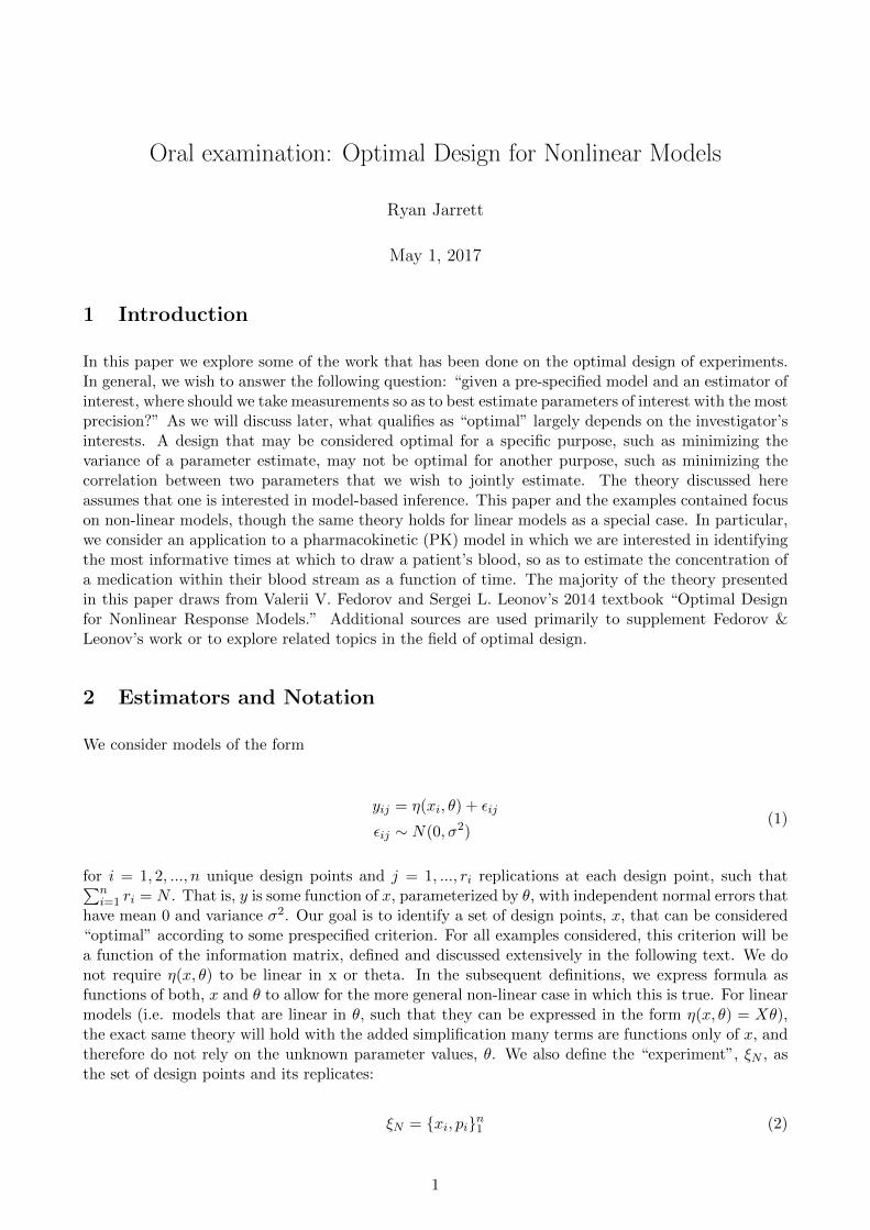
Oral examination: Optimal Design for Nonlinear Models

Ryan Jarrett

May 1, 2017

1 Introduction

In this paper we explore some of the work that has been done on the optimal design of experiments.In general, we wish to answer the following question: “given a pre-specified model and an estimator ofinterest, where should we take measurements so as to best estimate parameters of interest with the mostprecision?” As we will discuss later, what qualifies as “optimal” largely depends on the investigator’sinterests. A design that may be considered optimal for a specific purpose, such as minimizing thevariance of a parameter estimate, may not be optimal for another purpose, such as minimizing thecorrelation between two parameters that we wish to jointly estimate. The theory discussed hereassumes that one is interested in model-based inference. This paper and the examples contained focuson non-linear models, though the same theory holds for linear models as a special case. In particular,we consider an application to a pharmacokinetic (PK) model in which we are interested in identifyingthe most informative times at which to draw a patient’s blood, so as to estimate the concentration ofa medication within their blood stream as a function of time. The majority of the theory presentedin this paper draws from Valerii V. Fedorov and Sergei L. Leonov’s 2014 textbook “Optimal Designfor Nonlinear Response Models.” Additional sources are used primarily to supplement Fedorov &Leonov’s work or to explore related topics in the field of optimal design.

2 Estimators and Notation

We consider models of the form

yij = η(xi, θ) + εij

εij ∼ N(0, σ2)(1)

for i = 1, 2, ..., n unique design points and j = 1, ..., ri replications at each design point, such that∑ni=1 ri = N . That is, y is some function of x, parameterized by θ, with independent normal errors that

have mean 0 and variance σ2. Our goal is to identify a set of design points, x, that can be considered“optimal” according to some prespecified criterion. For all examples considered, this criterion will bea function of the information matrix, defined and discussed extensively in the following text. We donot require η(x, θ) to be linear in x or theta. In the subsequent definitions, we express formula asfunctions of both, x and θ to allow for the more general non-linear case in which this is true. For linearmodels (i.e. models that are linear in θ, such that they can be expressed in the form η(x, θ) = Xθ),the exact same theory will hold with the added simplification many terms are functions only of x, andtherefore do not rely on the unknown parameter values, θ. We also define the “experiment”, ξN , asthe set of design points and its replicates:

ξN = {xi, pi}n1 (2)

1

Oral examinationMay 1, 2017

where pi = ri/N . In the subsequent theory, in many cases to identify an optimal design we will allowpi to be continuous on the range (0, 1) and convert back to a whole number of replications at eachdesign point by multiplying ri = Npi. The gradient vector with respect to θ and the informationmatrix play a central role within the following theory and are defined as follows:

∂η(x, θ)

∂θ= ∇η (3)

We will denote the N × k dimensional gradient as ∇ηN , where N is the total number of observationsand k is the dimensionality of θ. The information matrix with respect to a single observation is

µ(x, θ) = σ−2∇η∇ηT (4)

The information matix is additive for i.i.d. observations, therefore the full information matrix for allN observations is given as

M(ξN , θ) = σ−2n∑i=1

riµ(xi, θ) (5)

We define D(ξN , θ) to be the inverse information matrix.

D(ξN , θ) = M(ξN , θ)−1 (6)

In the linear case, this is exactly equal to the variance-covariance matrix, while in non-linear casesit is an approximation to the variance-covariance matrix, with the degree of accuracy depending onthe closeness of the Taylor approximation of η(x, θ) about θ to the true function. It is useful in manycases to distinguish between the “Information Matrix” and the “Fisher Information Matrix,” wherethe former is defined as above, while the latter is defined as the negative expectation of the secondderivative of the log likelihood:

I(θ) = −Eθ[∂2ln p(x|θ)∂θ∂θT

]= −Eθ[H(θ)]

For linear models with normal errors, however, the information and Fisher information matrices co-incide with the value σ−2XTX. In the non-linear case with normal errors, the formula provided inequation 5 provides an approximation to the Fisher Information Matrix based on a first-order Taylorseries expansion. Derivations of the Fisher information matrices for the linear and nonlinear casesare provided in the Appendix. We also note that the information matrix is symmetric, non-negativedefinite matrix (i.e. all of its eigenvalues are greater than or equal 0),

zTM(ξN , θ)z = σ−2∑i

ri[zT∇η]2 ≥ 0 (7)

for any vector z ∈ Rm. It is also useful to introduce a normalized information matrix for all observa-tions:

M(ξN , θ) =

∫Xµ(x, θt)ξ(dx) (8)

Where ξ(dx) is the design weight given at value x. In the case where all design points are given equalweight, we have M(ξN , θ) = M(ξN , θ)/N .

2


●

●

●

●

●●

●

●

●

●

●

●

●

●

●

● ●

●●

● ●

●

●

●

●

●

●

●

●

●●

●

●

●

●

●

●

●

●

●

●

●

●

●

●

●

●

●

●●

0 1 2 3 4 5

−0.

20.

00.

20.

40.

60.

8f(x, θ) = θ1exp(− θ2x)

x

f(x,

θ)

Figure 1: Non-linear regression fit to generated data evaluated at the true values of theta.

3 Geometric Interpretation

All of the optimality criteria defined later in the paper are expressed as functions of the informationmatrix. Consequently, we believe it helpful to consider some of the geometric characteristics of theinformation matrix. For illustration, we consider the simple nonlinear model

yi = θ1e−θ2xi + εi

εi ∼ N(0, σ2)

with values {θ1 = 1, θ2 = 2, σ = 0.1, N = 50}. Our gradient vector is given

∇ηT = (e−θ2x,−θ1xe−θ2x)

and information matrix for N observations

M(ξN , θ) = σ−2∇ηTN∇ηN

Where ηN is a N × 2 matrix of gradient functions evaluated at each observation, x. The first-orderTaylor series expansion of η(x, θ) about θt is given

η(x, θ) = η(x, θt) + (θ − θt)∇η

We sample 50 random values of x uniformly on the bounds [0, 5] and generate corresponding valuesof y using the mean model and error described above. Using an iterative algorithm we calculatethe least-squares estimates, (θ1, θ2) = (0.87, 1.67). The generated data are shown in Figure 1 withthe line corresponding to the true model fit overlaid. The covariance matrix for the θ estimates is

3


1.0 1.5 2.0 2.5 3.0 3.5

0.6

0.8

1.0

1.2

1.4

Confidence region for θ1, θ2, R = 6

θ2

θ 1

●

●

●

True mean

NLLS Estimate

Samples from true distribution of NLLS estimator

Samples included in confidence ellipse about NLLS estimate

●

●

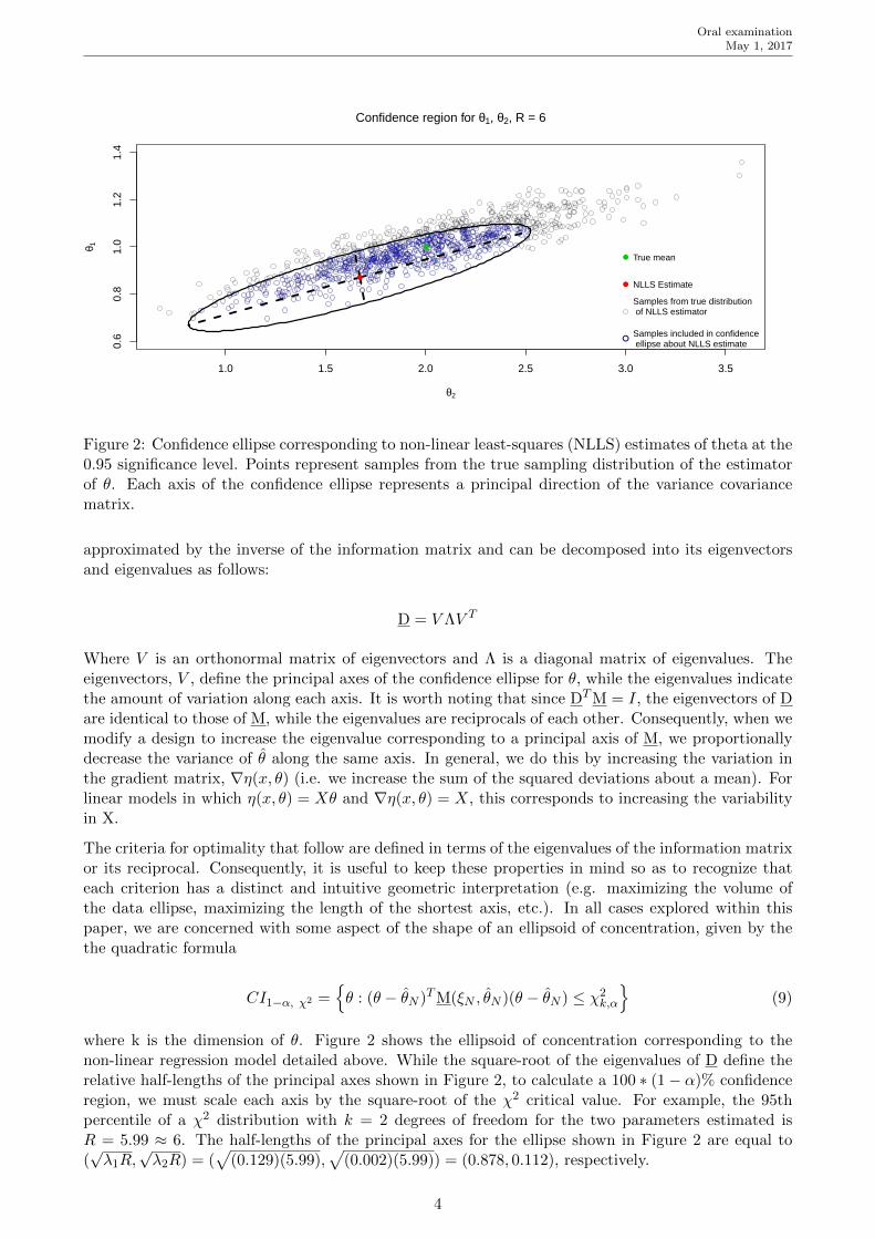
Figure 2: Confidence ellipse corresponding to non-linear least-squares (NLLS) estimates of theta at the0.95 significance level. Points represent samples from the true sampling distribution of the estimatorof θ. Each axis of the confidence ellipse represents a principal direction of the variance covariancematrix.

approximated by the inverse of the information matrix and can be decomposed into its eigenvectorsand eigenvalues as follows:

D = V ΛV T

Where V is an orthonormal matrix of eigenvectors and Λ is a diagonal matrix of eigenvalues. Theeigenvectors, V , define the principal axes of the confidence ellipse for θ, while the eigenvalues indicatethe amount of variation along each axis. It is worth noting that since DTM = I, the eigenvectors of Dare identical to those of M, while the eigenvalues are reciprocals of each other. Consequently, when wemodify a design to increase the eigenvalue corresponding to a principal axis of M, we proportionallydecrease the variance of θ along the same axis. In general, we do this by increasing the variation inthe gradient matrix, ∇η(x, θ) (i.e. we increase the sum of the squared deviations about a mean). Forlinear models in which η(x, θ) = Xθ and ∇η(x, θ) = X, this corresponds to increasing the variabilityin X.

The criteria for optimality that follow are defined in terms of the eigenvalues of the information matrixor its reciprocal. Consequently, it is useful to keep these properties in mind so as to recognize thateach criterion has a distinct and intuitive geometric interpretation (e.g. maximizing the volume ofthe data ellipse, maximizing the length of the shortest axis, etc.). In all cases explored within thispaper, we are concerned with some aspect of the shape of an ellipsoid of concentration, given by thethe quadratic formula

CI1−α, χ2 ={θ : (θ − θN )TM(ξN , θN )(θ − θN ) ≤ χ2

k,α

}(9)

where k is the dimension of θ. Figure 2 shows the ellipsoid of concentration corresponding to thenon-linear regression model detailed above. While the square-root of the eigenvalues of D define therelative half-lengths of the principal axes shown in Figure 2, to calculate a 100 ∗ (1− α)% confidenceregion, we must scale each axis by the square-root of the χ2 critical value. For example, the 95thpercentile of a χ2 distribution with k = 2 degrees of freedom for the two parameters estimated isR = 5.99 ≈ 6. The half-lengths of the principal axes for the ellipse shown in Figure 2 are equal to(√λ1R,

√λ2R) = (

√(0.129)(5.99),

√(0.002)(5.99)) = (0.878, 0.112), respectively.

4


1.0 1.5 2.0 2.5

0.6

0.7

0.8

0.9

1.0

1.1

1.2

Confidence region for θ1, θ2, R = 6

θ2

θ 1

●

4 Optimality Criteria

How do we define what constitutes an optimal design? Since the variance of our estimates is eithergiven or approximated by the inverse of the information matrix. Naturally, we may want consider adefinition of optimality of the form

ξ∗N = arg maxξN

M(ξN, θ) = arg minξN

D(ξN, θ) (10)

as such a criteria would minimize the variance of our estimates, θ. Since M(ξN), D(ξN) are matrices,we could understand maximizing or minimizing them in terms of a Loewner order, such that M(ξN) >M(ξ′N) if M(ξN) − M(ξ′N) is positive definite, and M(ξN) ≥ M(ξ′N) if M(ξN) − M(ξ′N) is positivesemi-definite. Intuitively, such a criteria would mean that the information matrix corresponding to anoptimal design has as much or more variation along all of its principal axes than those of all other sub-optimal designs. Fedorov and Leonov (2014), however, prove that even in the case of a simple linearregression, there does not exist a design that meets such a stringent optimality criterion. Instead, weare required to consider the minimization of a function, Ψ, of the information matrix:

ξ∗N = arg minξN

Ψ[M(ξN , θ)] (11)

4.1 Commonly used criteria

Commonly used optimality criteria include the following:

D-Optimality

Ψ = |D(ξN , θ)| = |M(ξN , θ)|−1 (12)

The D-optimality criterion minimizes the determinant of the variance-covariance matrix for θ and, indoing so, minimizes the area/volume of the the confidence ellipse. The determinant of the variance-covariance matrix is given by the product of the eigenvalues of D(ξN , θ). The volume/area of a dataellipse is proportional (proportionality constant π in 2 dimensions, 4π

3 in 3 dimensions) to the product

5

4.2 Approaches to parameter uncertaintyOral examination

May 1, 2017

of the root eigenvalues. For an arbitrary number of dimensions, the volume of the confidence ellipsoidis proportional to |D(ξN, θ)|1/2 and is given by the formula

Volume =πk/2

Γ(k/2 + 1)Rk/2|D(ξN, θ)|1/2

Where k is the dimensionality of θ and R is the bound of the ellipsoid, given by the χ2 critical valueassociated with the confidence ellipse in equation 9.

E-Optimality

Ψ = λ−1min|M(ξN, θ)| = λmax|D(ξN, θ)| (13)

In choosing the E-Optimality criterion, we minimize the largest eigenvalue of the variance-covariancematrix. In doing so, we aim to shorten the longest axis length of our confidence ellipse, thereby mini-mizing the largest variance associated with any linear combination of the parameter estimates.

A-Optimality

Ψ = tr|AD(ξN , θ)| (14)

Where A is a nonnegative definite matrix, referred to as a utility matrix. When A is a diagonal matrixwith non-negative elements, the A-Optimality criterion minimizes the weighted average variance ofthe parameter estimates with the jth weight given by the jth diagonal element of A divided by thetrace of A. In the case where A is the identity matrix, this geometrically corresponds to minimizingthe volume of the k-dimensional hyperrectangle (in our example, the 2-dimensional rectangle) thatcontains the confidence ellipse.

We present these criteria primarily to illustrate that there exist many properties of the confidenceellipse that we may wish to optimize, and that an “optimal” design depends on which properties ofan estimator one is interested in. For the sake of succinctness, the remainder of the paper will focusexclusively on the D-criterion, as it is the most widely used. However, the approach to identifying anoptimal design is similar for other optimality criteria.

4.2 Approaches to parameter uncertainty

For nonlinear models the optimality criteria is a function of the unknown parameters, θ. We must,therefore, find some way to account for this uncertainty. The simplest approach is referred to as a“locally optimal” design, in which one plugs in a guess, θ0, for θ. While straightforward, this approachfalls somewhat short of inspiring confidence in the resulting design if the design points are sensitiveto the values of θ and we are not certain of our chosen values of θ. Another approach is to use a“minimax” design, in which one finds the design that minimizes the design criterion at the parametervalue that maximizes the criterion. In this sense, we find the best design at the worst possible valuesof θ.

ξ∗N = argminξN

maxθ∈Θ

Ψ[M(ξN , θ)] (15)

Another approach is to minimize the average criterion value by integrating over an assumed distribu-tion for the unknown parameter:

6

4.3 Necessary and sufficient conditions for optimalityOral examination

May 1, 2017

ξ∗N = argminξN

∫Θ

Ψ[M(ξN , θ)]A(dθ) (16)

where A(dθ) is a prior distribution on θ.

It is also possible to adaptively estimate θ based on sequential sampling (Fedorov & Leonov, 2014).The general approach is to guess at θ0 and sample according to the optimal design under θ0, estimateθ from the first set of experiments, and update the optimal design based on θ. We consider later asampling approach, suggested by Matt Shotwell, in which the optimal design points are identified fora set of parameter values, drawn randomly from the prior distribution. The primary benefit of thisapproach is that it allows one to identify the design points that are robust to chosen parameter values,and illustrates the degree of variablilty in the design points that are not robust to parameter values.

4.3 Necessary and sufficient conditions for optimality

For a specific design to be optimized, it is necessary and sufficient for it to meet the following fourcriteria (Fedorov & Leonov, 2014):

1. Ψ(M) is a convex function, where covexity is defined such that if M = (1− α)M1 + αM2, then

Ψ(M) ≤ (1− α)Ψ(M1) + αΨ(M2) (17)

2. Ψ(M) is a monotonically non-increasing function, such that if M ≥M ′ in terms of Lowener ordering,then Ψ(M) ≤ Ψ(M′).

To reiterate, M ≥ M′ in Lowener ordering if the eigenvalues of M −M′ ≥ 0. In practice, due to theadditivity of the information matrix, M becomes larger in Lowener ordering as additional observationsare made. Consequently, as N increases, M never decreases in terms of Loewner ordering.

3. Let Ξ(q) = {ξ : Ψ|M(ξ)| ≤ q <∞} Then there exists a real number q such that Ξ(q) is non-empty.

This assumption merely requires that designs considered have a finite value of the chosen optimalitycriterion.

4. For any ξ, ξ ∈ Ξ(q)

Ψα(ξ, ξ) = Ψ[(1− α)M(ξ) + αM(ξ)] = Ψ[M(ξ)] + α

∫Xψ(x, ξ)ξ(dx) + o(α|ξ, ξ) (18)

where limα→0

o(α|ξ,ξ)α = 0 and 0 ≤ α ≤ 1.

In plain terms, this assumption states that for any two designs, ξ and ξ, the value of the optimalitycriterion associated with a weighted sum of the two corresponding information matrices can be ex-pressed as the optimality criterion of one design plus a weighted measure of distance or dissimilaritybetween the two designs. The amount of weight is given by α, while the “distance” is what is calleda directional (Gateaux) derivative (plus a remainder that tends to 0 as α becomes smaller). Theassumption requires that the directional derivative with regard to the optimality criterion functiontakes the form

∂Ψα(ξ, ξ)

∂α=

∫Xψ(x, ξ)ξ(dx) (19)

7


Intuitively, the directional derivative (i.e. the terms after α) tells us how much of a change in theoptimality criterion value is associated with a movement from design ξ to design ξ across the entiresupport of X , while α tells us the magnitude of the change. Under the integral, ψ(x, ξ) tells usthe magnitude of the change in Ψ(ξ) associated with a small increase in weight at point x and acorresponding decrease in weight at other values. ξ(dx) provides the weight given to point x by thedesign ξ. By integrating the change at each value, x, times the weight given to point x by design ξover the support X , we calculate the approximate change in the optimality criterion associated withan α−weighted shift from design ξ to design ξ.

For each of the common criteria, the directional derivatives have known forms and are merely presentedhere, though a derivation for the D-criterion is given in the Appendix.

ψD(x, ξ, θ) = m− tr[M−1(ξ, θ)µ(x, θ)] (20)

where m is the number of estimated parameters and µ(x) is the information matrix for a singleobservation, given by equation 4. The sensitivity function for the D-criterion is defined as

d(x, ξ, θ) = −ψD(x, ξ, θ) +m = tr[M−1(ξ, θ)µ(x, θ)] (21)

For E and A optimality, it is given by

ϕ(x, ξ, θ) = −ψ(x, ξ, θ) + Ψ(ξ, θ) (22)

The sensitivity function plays a large role in the search for and identification of optimal designs,detailed below.

5 Identification of an Optimal Design

A variety of methods can be used to identify an optimal design. If the number of design points, N, issufficiently small and the support of X is discrete (or can be discretized), then a brute-force calculationof the optimality criterion at all combinations could be used to find the design that minimizes theoptimality criterion. In many cases, however, this approach is infeasible. When N is large but thesample space is discrete, various search algorithms can be used to find an optimal design.

5.1 Equivalence theorems

For the optimality criteria listed above, there exist “Equivalence Theorems,” which express optimalitycriteria in alternate forms that can quickly verify whether or not a design is optimal. For example,for the D-criterion, the following criteria were shown to be equivalent (Kiefer-Wolfowitz, 1960):

1. minξ|D(ξ, θ)|2. minξmaxxd(x, ξ)

3. maxxd(x, ξ) = m

(23)

Where d(x, ξ) is the sensitivity function for the D-optimality criterion, defined in equation 21. Similarequivalence theorems can also be stated for other commonly used criteria, but are omitted here.Primarily, we will concern ourselves with the first and third forms of the equivalence theorem, whichstate that the determinant of the variance-covariance matrix is minimized when the maximum of thesensitivity function on the support of x is equal to the number of parameters in the model, m. It is

8

5.2 Algorithm for identificationOral examination

May 1, 2017

worth noting, however, that d(x, ξ, θ) is approximately equal to the variance of the estimated response(equal in the linear case), and reaches its minimum at d(x, ξ, θ) = m. Therefore, in finding a D-optimaldesign, in addition to minimizing the volume of the confidence ellipse around our estimated parameters,the maximum variance of the estimated response is also minimized. A proof of the equivalence of thesensitivity function and the variance of the predicted response is given in the appendix.

5.2 Algorithm for identification

Though faster algorithms are available, we choose a relatively simple procedure for finding an optimaldesign, as described by Federov and Leonov’s forward and backward iterative procedures. The processconsists of iteratively finding the points on the support of x at which the value of the sensitivity functionis the highest and lowest. These points are then up-weighted and down-weighted, respectively in thenext iteration by a scalar, αs, that varies with each iteration.

For each iteration until convergence of Ψ(M) within some tolerance we apply the following algorithm:

1. Given the design at the sth iteration, ξs, find the points that maximize and minimize the sensi-tivity function, respectively:

x+s+1 = arg max

xd(x, ξs)

x−s+1 = arg minx

d(x, ξs)

2. Add the point x+s+1 to the design with weight α+

s .

ξ+s = (1− α+

s )ξs + α+s ξ(x

+s+1)

Fedorov & Leonov show the α that achieves the steepest descent (i.e. it minimizes the optimalitycriterion evaluated at the resulting design) to be

α+s = arg min

α|D(ξs+1)| =

d(x+s+1, ξs)−m

[d(x+s+1, ξs)− 1]m

3. Down-weight x−s+1 in the design ξ+s

ξs+1 = (1− α−s )ξ+s + α−s ξ(x

+s+1)

Where

α−s = −min

(α+s ,

ps1− ps

)and ps is the weight given to point x−s+1 in design ξs.

We initiate the algorithm with a design, ξ0, that uniformly distributes sampling weight over thesupport of x. As a practical consideration, while the design weight, ξ, is a continuous quantity, thesupport of x must be descretized at some level of precision; however, this is not a major concern inthe identification of design points in practice. For example, if one wishes to identify the optimal timepoints at which to draw a patient’s blood, it is likely sufficient to consider time as discretized intominute-long intervals. The only cost associated with discretizing to increasingly granular intervals isadditional computing time.

9


6 Application to Pharmacokinetics Data

We now consider an application of these methods to a Pharmacokinetics (PK) example. Here, weare interested in identifying the times at which a patient’s blood should be drawn to most accuratelyestimate the drug concentration over time, given a pre-specified dosing schedule. A two-compartmentdifferential equation model is used to describe the dynamics of the drug within an individual. Thismodel allows for a central compartment (i.e. bloodstream), with a mass of the drug given by m1, anda peripheral compartment (i.e. tissue) with mass m2. The two compartments have volumes v1 andv2, respectively. The rates of diffusion from the central to the peripheral is defined as k12, and fromthe peripheral to the central as k21. An elimination rate from the central component is given by theparameter k10. The drug infusion rate is given by kR and is assumed to be known, as this is controlledby the experimenter/physician. For the present example, kR is a piecewise function of time, takingon a positive constant value while the drug is being infused intravenously, and 0 for all other times.The model can be expressed as a system of two equations relating the change in drug concentrationwithin each compartment over time to the four unknown PK parameters, {v, k12, k21, k10}.

dm1

dt= kR + k21m2 − k12m1 − k10m1

dm2

dt= k12m1 − k21m2

(24)

The mass in the two compartments can easily be converted to a concentration by dividing by thevolumes of the respective compartments: c1 = m1/v1 c2 = m2/v2. In practice, we typically observe ameasurement of c1, the concentration of the drug within the main compartment (i.e. bloodstream).The solutions to this set of equations provide models of the total drug concentration in a patient’sbody as a function of time. A derivation of the solution is provided in the Appendix. We assume themeasured drug concentration in the central compartment at time t to be normally distributed aboutthe value predicted by the solution for c1(t) in the above differential equations with variance σ2.

c1(t) ∼ N(g(t, v1, k10, k12, k21), σ2) (25)

Estimates of population PK parameters and σ2 from a previous study are used to create prior distribu-tions for the PK parameters and error variance, respectively. These prior distributions are, therefore,best thought of the estimated variability within the population, rather than our state of uncertaintyregarding their true values, as we frequently use priors to represent. Specifically, we use the followingprior distributions:

{lnv1, lnk10, lnk12, lnk21} ∼ N4

µ0 =

3.223−1.650−5.000−5.000

,Σ0 =

0.501 −0.384 0.000 0.000−0.384 0.462 0.000 0.0000.000 0.000 0.045 0.0000.000 0.000 0.000 0.045

ln(σ) ∼ N(2.33, 0.32)

(26)

An example central concentration curve as a function of time for a fixed set of prior parameters withsimulated observations is given in Figure 3. In the figure, PK parameter values and an error termare drawn from the prior distribution specified. This set of parameter values can be thought of ascharacterizing the pharacokinetic profile of a hypothetical patient within the population of patientsdescribed by the prior distribution. The patient then receives 5 intravenous doses, with each infusionlasting 3 hours. The dosing interval (i.e. the time between the starts of consecutive infusions) is setat 8 hours, with measurements are taken during the fifth dosing period at t = (32, 32.5, 33, 34, 36,38) hours.

10


0 10 20 30 40

0.00

0.10

0.20

0.30

Time (h)

Cen

tral

Con

cent

ratio

n (g

/L)

●

●●

● ●

●

Figure 3: Example concentration curve for PK parameters drawn from prior distribution with simu-lated data.

0 2 4 6 8

1.5

2.0

2.5

3.0

3.5

4.0

8 hour dosing interval, 3h infusion duration

Time since start of last infusion (h)

Sen

sitiv

ity, d

(θ,ξ

)

0 2 4 6 8

0.00

0.10

0.20

0.30



Des

ign

wei

ghts

, ξ(d

x)

Using this model, we conduct what is, in essense, a simulation study in which we identify the op-timal design corresponding to a hypothetical population of 50 patients. In theory, each patient’spharmacokinetic profile is fully characterized by a set of parameters drawn from the prior distributionspecified above. The response function, η(x, θ), is given by the solution to the differential equationmodel for the central compartment, which then describes the drug concentration in the bloodstreamas a function of time. The gradient function and information matrix are numerically approximatedand we initialize the algorithm described in Section 5.2 with a design that assigns equal weight to alltime points. For each simulated patient, the algorithm is iterated until convergence and the resultingsensitivity function is checked to verify that its maximum on the support of x is equal to m = 4. Theequivalence theorems provided earlier provide that this is equivalent to an optimal design (i.e. one

11


0 2 4 6 8

1.5

2.0

2.5

3.0

3.5

4.0



Sen

sitiv

ity, d

(θ,ξ

)

0 2 4 6 8

0.00

0.10

0.20

0.30



Des

ign

wei

ghts

, ξ(d

x)

0 2 4 6 8 10 12

1.5

2.0

2.5

3.0

3.5

4.0



Sen

sitiv

ity, d

(θ,ξ

)

0 2 4 6 8 10 12

0.00

0.10

0.20

0.30



Des

ign

wei

ghts

, ξ(d

x)

0 5 10 15 20

1.5

2.0

2.5

3.0

3.5

4.0



Sen

sitiv

ity, d

(θ,ξ

)

0 5 10 15 20

0.00

0.10

0.20

0.30



Des

ign

wei

ghts

, ξ(d

x)

Figure 4: D-optimal design points at different dosing intervals for 5th infusion at 3 hour infusionduration (shaded grey). Each line represents a draw from the prior distribution of PK parameters.Optimal design points are colored blue. Left hand panels show the sensitivity function values associatedwith the optimal design for each set of parameters. Right hand panels show the corresponding designweights for each optimal design.

that minimizes the determinant of the variance-covariance matrix). The results of these simulationsare shown in Figure 4.

The sensitivity functions in the left hand panels of Figure 4 show that for each hypothetical patientthere exist 5 design points for the 8 hour and 12 hour dosing intervals, and either 4 or 5 design points inthe 24 hour dosing interval. The blue points in Figure 4 indicate the locations at which the sensitivity

12


function is equal to m. The right hand panels show the design weights associated with the set of50 optimal designs (one for each set of parameters). In all panels of the figure, lines are drawn witha degree of transparency, such that darker areas indicate agreement across sets of parameters. Forexample, in the top left panel of Figure 4, design points are located at 0, 3, and 8 hours following thebeginning of the final infusion across all 50 “patients.” The final two design points are placed roughlyat 1.75 and 4.5 hours and show sensitivity to parameter specification.

The portion shaded grey indicates the time during which the drug was administered intravenously. Inall dosing scenarios, the same mass of drug was given to each patient, but was given at different ratesto account for varing sizes of the dosing windows. In general, the most consistently informative pointsfor each patient occur at the beginning and end of the dosing interval, as well as at the end of theinfusion period. The remaining design points occur mid-infusion and after approximately a third ofthe time between the end of the infusion and the end of the dosing interval has passed, though thesedesign points demonstrate variability between patients.

7 Discussion

7.1 Limitations

There are several limitations of the theory discussed in this paper. The most obvious is that thenumber of design points is a function of the model under consideration and – in the PK example– the dosing schedule. Consequently, while the theory may provide the optimal weight assigned toeach design point, for fixed sample sizes that are not multiples of the number of design points, it isunclear where the remaining measurements should be taken. Box and Lucas (1959) suggest alternatelyusing additional observations to estimate additional parameters in a more general model as a meansof model-checking, or to better estimate specific areas of the response surface that the investigator(perhaps due to intuition) believes to be poorly estimated. For a given sample size, however, wecan measure the information loss due to discretization of the design. This can be done simply bycalculating the relative D-efficiency as follows:

D-eff(ξ) =|M(ξ, θ)|1/k

|M(ξ∗, θ)|1/k(27)

Using this approach, we can see how various designs with a fixed N compare to the optimal designand choose the one that minimizes the relative information loss if we are confident in our modeland parameter values. It is worth emphasizing, however, that there are various reasons that onemay not wish to choose the design that minimizes the relative information loss. In addition to theconsiderations of Box and Lucas, we may wish to emphasize robustness in choice of θ values. Thesampling approach used in the PK example above illustrates that not all design points are equallyrobust to parameter misspecification. Consequently, one may reasonably wish to choose a design thatgives higher weight to the support points that were invariant to θ. Approaches such as the minimaxand averaging methods do not allow one to view this sensitivity to parameter misspecification.

A additional issue common to nonlinear regression models is that the space of the response function,η(x, θ), is curved with respect to θ, allowing for situations in which ||η(x, θ)− η(x, θ0)|| is small evenwhen the distance between θ and θ0 is large. In practice, this translates to the frequent presence oflocal optima which can cause the estimator to be non-unique or highly sensitive to small changes in theobservations. Pazman and Pronzato (2013) introduce a generalized form of the E-optimality criterion(as well as c-optimality and G-optimality, which are not discussed in this paper) that mitigates thisrisk by incorporating a Euclidian distance measure between θ and θ0 into the optimality criterion.

13

7.2 ExtensionsOral examination

May 1, 2017

7.2 Extensions

The optimal design theory presented has been extended in diverse ways which we will only brieflymention here. Federov and Leonov (2014) show that constraints, such as the costs associated with thecollection of data points, can be incorporated into the existing theory. The general principal behinddoing so is to define a cost function associated with each design point

Φ(ξN , θ) =

n∑i=1

riφ(xi, θ)

which is then incorporated into the optimality criterion:

ξ∗ = argminξ

Ψ

[M(ξ, θ)

Φ(ξ, θ)

]Additional applications include the identification design points to simutaneously discriminate betweena set of candidate models and estimate the parameters of the selected model. This is achieved throughthe use of the T-optimality criterion, in which one posits a true model and a set of rival models andchooses the design so as to maximize the sum of squares for lack of fit for the rival model(s) (Atkinson& Fedorov, 1975a,b). One then uses a likelihood ratio test to select a model.

Adaptive designs based on repeated experiments have been developed and are commonly used in dose-finding clinical trials (Federov & Leonov, 2014; Lane, 2013). During adaptive designs, the parametersat each stage are reestimated using data from prior stages to find updated design points. Given thatthe identification of an optimal design for nonlinear models depends on the model parameters, θ, whichare rarely (if ever) known in advance, when repeated experimentation is possible, adaptive designstypically provide a superior alternative to locally optimal designs.

Extensions have also been made into the optimal design of experiments for nonparametric models, inwhich the form of the response function is unspecified beyond smoothness and regularity properties.Muller (1984) introduced a locally optimal design criterion for nonparametric (kernel density) regres-sion models, which was extended by Biedermann and Dette (2000) to allow for a minimax approach.The latter authors find that in certain cases, uniform weights along X is optimal. In these scenarios,since kernel density models are parameterized by a bandwidth tuning parameter, a “locally optimal”design refers to one in which the bandwidths are known. In practice, if bandwidths are permitted tovary along the support of the design variable, an optimal design will depend on the selection of thebest values for these bandwidths, which are typically unknown.

According to Pronzato & Pazman (2013), since the response function is unknown in nonparametricscenarios, the optimal design is typically that which places design points so as to “have a space-filling property.” When our set of design variables is one dimensional and we use a euclidian distancemeasure, which we may choose to use when we have no prior information regarding the value of theresponse function over support of our design variable, this translates to sampling uniformly across X .In higher dimensions, however, “space-filling” is not as simple and may be defined in various ways (e.g.which is preferable, a square grid or a triangular grid?) (Pronzato & Muller, 2011). For example, onemay choose to maximize the distance (on any measure) between each point and its closest neighbor, inwhat is called a “maximin-distance design,” or one may minimize the maximum distance between allpoints and their closest neighbor in a “minimax-distance design.” Many additional approaches existand, as before, what can be considered optimal will depend on one’s interests.

Many questions of interest in statistics do not allow for an experimental setting in which the researcheris able to collect data at pre-determined design points. For those that do, however, the identificationof points that are likely to confer the most information to a researcher’s candidate model can result inincreased estimate efficiency and is worth consideration in the design stage of a trial or experiment.

14

REFERENCESOral examination

May 1, 2017

References

[1] Atkinson, A. C. & Fedorov, V. V. The Design of Experiments for Discriminating Between twoRival Models. Biometrika, Vol. 62, No. 1 (Apr., 1975), pp. 57-70

[2] Atkinson, A. C. & Fedorov, V. V. Optimal Design: Experiments for Discriminating betweenSeveral Models. Biometrika, Vol. 62, No. 2 (Aug., 1975), pp. 289-303

[3] Biedermann, S. & Dette H. Minimax optimal designs for nonparametric regression - a furtheroptimality property of the uniform distribution. In A. Atkinson, P. Hackl, and W. Muller (Eds.),mODa’6 – Advances in Model–Oriented Design and Analysis, Proc. 6th Int. Workshop, Puch-berg/Schneberg (Austria), Heidelberg, pp. 13–20. Physica Verlag.

[4] Box, G. E. P. & Lucas, H. L. (1959) Design of Experiments in Non-Linear Situations. Biometrika.46:77-90.

[5] Fedorov, V. V., & Leonov, S. L. (2014). Optimal design for nonlinear response models. BocaRaton: CRC Press/Taylor & Francis Group.

[6] Kiefer, J. & Wolfowitz, J. (1960). The equivalence of two extremum problems. Canad. J. Math.,12:363–366

[7] Lane, A., Yao, P., Flournoy, N. (2013). Information in a two-stage adaptive optimal design Journalof Statistical Planning and Inference 144 (2014) 173–187

[8] Muller, Hans-Georg (1984). Optimal Designs for Nonparametric Kernel Regression Statistics &Probability Letters 2 (1984) 285-290

[9] Pazman A. & Pronzato L. (2013) Extended Optimality Criteria for Optimum Design in Non-linear Regression. Advances in Model-Oriented Design and Analysis. Contributions to Statistics.Springer, Heidelberg.

[10] Petersen, K. B. & Pedersen, M. S. (2012). The Matrix Cookbook. Technical University of Den-mark.

[11] Pronzato L. & Pazman A. (2013) Design of Experiments in Nonlinear Models: Asymptotic Nor-mality, Optimality Criteria and Small-Sample Properties. Springer-Verlag, New York

[12] Pronzato L. & Muller, W. (2012). Design of computer experiments: space filling and beyond.Springer Verlag (Germany), 2012, 22 (3), pp.681-701.

[13] von Gilbert Koch, vorgelegt (2012). Modeling of Pharmacokinetics and Pharmacodynam-ics with Application to Cancer and Arthritis Department of Mathematics and Statistics,University of Konstanz http://www.math.uni-konstanz.de/numerik/personen/koch/papers/Diss Koch Final.pdf

15


8 Appendix

8.1 Derivations of Information Matrices

Given the model

y = η(x, θ) + ε

ε ∼ N(0, σ2)

the log likelihood function is

l(θ) = −1

2ln(2πσ2)− −(y − η(x, θ)2)

2σ2

and corresponding score function

∂lθ

∂θ= S(θ) =

(y − η(x, θ))∇ησ2

In the linear case, ∇η = x, and the score function reduces to

S(θ) =(y − xT θ)x

σ2

The Hessian is given by

∂S(θ)

∂θ= H(θ) = −xx

T

σ2

And the Fisher Information Matrix by the negative expectation of the Hessian

I(θ) = −Eθ[H(θ)] =xxT

σ2

Which coincides with the information matrix for the least-squares estimator. In the non-linear case,we make a first-order Taylor series approximation about the true value of θ, θt:

η(x, θ) ≈ η(x, θt) + (θ − θt)T∇η

Substituting this approximation into the initial model

y − ε = η(x, θt) + (θ − θt)T∇ηy − η(x, θt) + θTt ∇η = θT∇η + ε

y∗ = θT∇η + ε

Which is linear in θ and of the same form as the linear model described above. The steps to calculatethe Fisher information matrix are identical and we end up with

I(θ) ≈ (∇η)T (∇η)

σ2

Similarly, for nonlinear least-squares

16

8.2 Derivation of sensitivity function for D-criterionOral examination

May 1, 2017

θ = (∇ηT∇η)−1∇ηT y∗

V (θ) ≈ σ2(∇ηT∇η)−1

In both the maximum likelihood and the least-squares approaches, iterative algorithms can be usedto solve for θ and V (θ), where the estimate at each step is substitued in for the “true” value, θt. Theaccuracy of the estimated information matrix in the non-linear case is obviously dependent upon theappropriateness of the first order Taylor series approximation.

8.2 Derivation of sensitivity function for D-criterion

As stated previously, the directional derivative associated with the fourth necessary and sufficientcondition for optimality takes the form

∫Xψ(x, ξ)ξ(dx)

The general form of the sensitivity function is

ϕ(x, ξ) = −ψ(x, ξ) + C

where C is equal to the number of parameters estimated, m, for the D-criterion and is equal to Ψ(ξ)for all other criterion. An α-weighted design with respect to arbitrary designs ξ, ξ is given as

ξα = (1− α)ξ + αξ = ξ + α(ξ − ξ)

with a corresponding information matrix

Mα = (1− α)M(ξ) + αM(ξ) = M(ξ) + α(M(ξ)−M(ξ))

To find ψ(x, ξ) for a specific optimality criterion, we calculate the derivative of our optimality criterionfor an α-weighted design with respect to α and evaluate the limit as α→ 0.

17

8.3 Equivalence of sensitivity function and variance of predicted responseOral examination

May 1, 2017

Ψα = −ln|Mα|dΨα

dα= Ψ′α = −tr

{M−1α

dMα

dα

}(Matrix cookbook, eq.43)

= −tr{M−1α [M(ξ)−M(ξ)]

}= −tr

{[M(ξ) + α(M(ξ)−M(ξ)]−1[M(ξ)−M(ξ)]

}limα→0

Ψ′α = Ψα = −tr{M(ξ)−1[M(ξ)−M(ξ)]

}(Interchange limit and summation)

= −tr{M(ξ)−1

[∫µ(x)ξ(dx)−

∫µ(x)ξ(dx)

]}= −tr

{M(ξ)−1

[∫µ(x)ξ(dx)−

∫∫µ(x)ξ(dx)ξ(dx)

]} (∫ξ(dx) = 1

)= −tr

{M(ξ)−1

[∫ξ(dx)

[µ(x)−

∫µ(x)ξ(dx)

]]}= −tr

{∫ξ(dx)

[M(ξ)−1µ(x)−M(ξ)−1M(ξ)

]}=

∫ξ(dx)

[−tr(M(ξ)−1µ(x)) +m

]=

∫ξ(dx)

[m− tr(M(ξ)−1µ(x))

]Therefore,

ψ(x, ξ) = m− tr(M(ξ)−1µ(x))

Giving us the sensitivity function for the D-criterion:

ϕ(x, ξ) = tr(M(ξ)−1µ(x))

The limit and trace operators can be interchanged during the derivation by the Dominated Conver-gence Theorem. The trace of fα = M−1

α [M(ξ)−M(ξ)] is a summation of m positive and finite values,all of which can be bounded by merely adding a constant to each: gα = fα + c. Since fα can bebounded by another function, gα, with a finite sum, the theorem applies and we have

limα→0

tr(fα) = tr(f)

8.3 Equivalence of sensitivity function and variance of predicted response

We wish to show that the sensitivity function for the D-criterion, given as

tr[M−1(η, θ)µ(x, θ)]

is approximately equivalent to the variance of the predicted response, η(x, θ). We begin by evaluatingthe variance of the Taylor series approximation to the predicted response (i.e. using the multivariatedelta method).

18

8.4 Solution to differential equation modelOral examination

May 1, 2017

η(x, θ) ≈ η(x, θ) + (θ − θ)∇ηV (η(x, θ)) ≈ V (η(x, θ) + (θ − θ)∇η)

= V (θ∇η)

= ∇ηTD∇η

= (∇η1, ...,∇ηk)

D11 . . . D1k...

. . ....

Dk1 . . . Dkk

∇η1

...∇ηk

= ∇η1

k∑j=1

∇ηjDj1 + ...+∇ηkk∑j=1

∇ηjDjk

=k∑i=1

Dii∇η2i +

∑i

∑j 6=i

Dij∇ηi∇ηj

We can then see that this expression is identical to the sensitivity function for the D-criterion

tr[M−1(η, θ)µ(x, θ)] = tr[M−1(η, θ)∇η∇ηT ]

= tr

D11 . . . D1k

.... . .

...Dk1 . . . Dkk

∇η2

1 . . . ∇η1∇ηk...

. . ....

∇ηk∇η1 . . . ∇η2k

= tr(S)

The diagonal elements of the matrix S are given

S11 = D11∇η21 +D12∇η2∇η1 + ...+D1k∇ηk∇η1

S22 = D21∇η1∇η2 +D22∇η22 + ...+D1k∇ηk∇η2

...

Skk = Dk1∇η1∇ηk + ...+Dk,k−1∇ηk−1∇ηk +Dkk∇η2k

When summed, these equal

tr(S) = S11 + S22 + ...+ Skk =k∑i=1

Dii∇η2i +

∑i

∑j 6=i

Dij∇ηi∇ηj

8.4 Solution to differential equation model

Here we derive the solution to the two-compartmental differential equation model presented for a singledosing period. The general approach to the derivation follows the example of vorgelegt von GilbertKoch (2012), who uses the Laplace transform method to find the solution for the homogenous linearsystem (i.e. without the drug infusion rate, kR). The concentration across multiple dosing periods isgiven by a piecewise function with the initial concentration in the primary compartment given by theconcentration at the conclusion of the prior dosing period.

The system of equations, expressed in terms of volume rather than concentration and without theinitial infusion is given

19


May 1, 2017

dx1

dt= x′1(t) = −(k10 + k12)x1(t) + k21x2(t) + kR

dx2

dt= x′2(t) = k12x1(t)− k21x2(t)

(28)

and can be expressed in matrix form as

x′(t) = Ax(t) +R

In which

x′(t) =

(x′1(t)x′2(t)

)A =

(−(k10 + k12) k21

k12 −k21

)x(t) =

(x1(t)x2(t)

)R =

(kR0

)The Laplace transform of a function, f(t) is given

L(f(t)) =

∫ ∞0

f(t)e−stdt ≡ F (s)

We note the following properties to be used:

1. L(A) = As by direct calculation.

2. L(Ax(t)) = AX(s) by definition.

3. L(x′(t)) = sX(s)− x(0) by direct calculation using integration by parts.

We now apply the Laplace transform to both sides

x′(t) = Ax(t) +R

L(x′(t)) = L(Ax(t)) + L(R)

sX(s)− x(0) = AX(s) +R(s) R(s)T = (kR/s, 0)

(sI −A)X(s) = x(0) +R(s)

X(s) = (sI −A)−1(x(0) +R(s))

We define

sI −A = M(s) =

(s+ k10 + k12 −k21

−k12 s+ k21

)such that

M−1(s) =1

(s+ k10 + k12)(s+ k21)− k12k21

(s+ k21 k21

k12 s+ k10 + k12

)We note that

(s+ k10 + k12)(s+ k21)− k12k21 = s2 + s(k10 + k12 + k21) + k10k21

= (s+ α)(s+ β)

where by the quadratic formula,

20


May 1, 2017

α, β =1

2

[k10 + k12 + k21 ±

√(k10 + k12 + k21)2 − 4k10k21

]and additionally that −α,−β are the eigenvalues of A, λ1, λ2.

M−1(s)(x(0) +R(s)) =1

(s+ α)(s+ β)

(s+ k21 k21

k12 s+ k10 + k12

)(kR/s+ x1(0)

x2(0)

)=

1

(s+ α)(s+ β)

((s+ k21)(kR/s+ x1(0)) + k21x2(0)

k12(kR/s+ x1(0)) + (s+ k10 + k12)x2(0)

)To take the inverse Laplace transform of M−1(s)(x(0)+R(s)), we can use Heaviside’s Theorem, whichstates

L−1

(p(s)

q(s)

)=

n∑i=1

p(λi)

q′(λi)eλit

where λi is the ith eigenvalue of A. To apply this theorem, we note that q(s) = (s + α)(s + β) andq′(s) = 2s+ α+ β.

we then can solve for the mass in the first compartment

x1(t) = L−1(X1(s)) = L−1(M−1(s)(x(0) +R(s)))

=

[sx1(0) + kRk21

s

q′(s)

∣∣∣s=−α

e−αt +sx1(0) + kRk21

s

q′(s)

∣∣∣s=−β

e−βt

]+

(kR + k21(x1(0) + x2(0)))

[q′(s)−1

∣∣∣s=−α

e−αt + q′(s)−1∣∣∣s=−β

e−βt]

=

[−αx1(0) + kRk21

−αβ − α

e−αt +−βx1(0) + kRk21

−βα− β

e−βt

]+[

kR + k21(x1(0) + x2(0))

β − αe−αt +

kR + k21(x1(0) + x2(0))

α− βe−βt

]=αkR − kRk21 + α[k21(x1(0) + x2(0))− αx1(0)]

α(β − α)e−αt+

βkR − kRk21 + β[k21(x1(0) + x2(0))− βx1(0)]

β(α− β)e−βt

At the start of the first infusion the inital mass in each compartment is equal to 0, such that x1(0) =x2(0) = 0 and the solution simplifies to

x1(t) =kR(k21 − α)

α(α− β)e−αt +

kR(k21 − β)

β(β − α)e−βt

The solution can be expressed in terms of the concentration within the central compartment at timet merely by dividing the mass of the drug in the central compartment at time t, x1(t), by the volumeof the central compartment, v1:

c1(t) =x1(t)

v1

21


9 Additional Graphics

●

●

●

●

●

●

●●

●

0.0 0.5 1.0 1.5 2.0 2.5 3.0

0.0

0.2

0.4

0.6

0.8

Sample points from design 1

x

f(x,

θ)

True curveEstimated curve

●

●

●

●

●

●

● ●

●

0.0 0.5 1.0 1.5 2.0 2.5 3.0

−0.

20.

00.

20.

40.

60.

81.

0


x

f(x,

θ)


●

● ●

●

●

●

●

●●

0.0 0.5 1.0 1.5 2.0 2.5 3.0

−0.

20.

00.

20.

40.

60.

81.

0


x

f(x,

θ)


0.5 1.0 1.5 2.0 2.5 3.0 3.5

0.6

0.8

1.0

1.2

1.4

Confidence region for design 1

θ2

θ 1

Volume = 0.567Longest axis = 2.101Shortest axis = 0.344Diagonal length = 2.129

●

●

True mean = (1, 2)NLLS Estimate = (0.937, 1.762)

●

●

0.5 1.0 1.5 2.0 2.5 3.0 3.5

0.6

0.8

1.0

1.2

1.4


θ2

θ 1


●

●


●

●

0.5 1.0 1.5 2.0 2.5 3.0 3.5

0.6

0.8

1.0

1.2

1.4


θ2

θ 1


●

●


●

●

22

Ryan Jarret - Vanderbilt University

Documents

Transcript of Ryan Jarret - Vanderbilt University