rW 1-fi - Defense Technical Information Center · tional support; to Paul Andry (physicist and...

n U - N

LAnD AT

T SCIENCE

.'5 rW 1-fi ST- 444

Unclassified

SECuRitY CLA$SIFICATIO. OF "-HIS PAU-

R R DOCUMENTATION PAGEM1, REPORT SECURITY CLASS'FI Io RES 1 RICTIVE MARKINGS

Unclssfied n E E T2. SECURITY CLASSIFICArION - RITJAN 1 1 1 3 0ISTRIIUTIONIAVAILASILITY OF REPORT2b OECLASSIFICATIONIOWN SCHE Approved for public release; distribution

%. is unlimited.

4, PERFORMING ORGANIZATION REPORT M S} 5 MONITORING ORGANIZATION REPORT NijUMER(S)

M!IFILCS/TR-467 N000l4-34-K-0099N00014-89-J-1988

64, NAME OF PERFORMING ORGANIZATION 6b OFFICE SYMBOL li NAME OF MONITORING ORGANIZAIION

:IT Lab for Computer Science Office of Naval Rezearch/Depc. of NAvy

6C. AOORESS (CRy, State. and ZIP Code) 7b, ADDRESS (City, Stare. and ZIP Code)

545 Yechnology Square Information Syscems Program

Cambridge, ,h 02139 Arlington, VA 22217

ft. NAME OF FUNODINGISPONSORING Sb, OFFICE SYMBOL 9, PROCUREMENT INSTRUMENT IDENTIFICATION NUMBERORGANIZATION (If apikable)DARPA/DOD

S .ADDRESS (City, State. and ZIPCode) 10. SOURCE OF FUNDING NUMBERSPROGRAM PROJECT TASK WORK UNIT

1400 Wilson B.lvd. ELEMENT NO. NO. NO ACCESSION NO,Arlingcon, VA 22217

II, TITLE (kiude Security Class ication)

A Scalable Multiprocessor Architecture Using Cartesian Network-Relative Addressing

12. PERSONAL AUTHOR(S)Morrison, Joseph Derek

13a, TYPE OF REPORT 13b, TIME COVERED 14, DATE OF REPORT (Year.Month, Day) IS PAGE COUNTTechnical FROM ____ TO 1989 December 139

16, SUPPLEMENTARY NOTATION ;,,. ,

17 COSATI CODES 1 1S, SUBJECT TERMS (Continue on revene If necetuty and identify by block number)FIELD GROUP SUB.GROUP "-ult Jtprocesso r calability;% -.rte ian- itopology, add ress

space; relative addressing; task migracion; parallelism, .

19, ABSTRACT (Continue on reverse if neceuary an identify by block number)- The Computer Architecture Grop<t-the.Lab .ratory-for.Computer-Science$s developing

a new model of computation called . 'his thesis describes a highly scalable archhecturefor implementing k£called Oartesian-Network-Relative-Addressing(NRA4'

In the CNRA architecture, processor/memory pairs are placed at the nodes of a low.dimensional Cartesian grid network. Addresses in the system are composed of a'ioutin- "component which describes a relative path through the interconnection network (the originof the path is the node on which the address resides), and L"emor ioi oben- -which specifies the memory location to be addressed on the node at the destination of therouting path.

The CNRA addressing system allows sharing of data structures in a style similar to thatof global shared memory machines, but does not have the disadvantages normally associated -,

20 DISTRIBUTIONIAVAILABILITY OF ABSTRACT 21 ABSTRACT SECURITY CLASSIFICATION13 UNCLASSIFIEDIUNLIMITED 0 SAME AS RPT J] OTIC USERS Unclassified

22a NAME OF RESPONSIBLE INDIVIDUAL Z2b TELEPHONE (Include Area Code) I 22c, OFFICE SYMBOL1udv Little (617) 253-5894

DD FORM 1473, 84 MAR 83 APR edition may be used until exhausted SECURITY CLASSIFICATION OF THIS PAGEAll other editions are obsolete

iU. Gowtnm t PAi6i. OffHIO: IM-07.047Unclassified90 01 10 135

use -I""'

-,with shared-memory machin .., (i.e. l;dLtcd address space and'mcnory access latency thatincreases with system size).

This thesis discusses how a przctical CNRA syjtem might be built. There are discussionsiRihow the system software might manage the~e~rlative pointers'in a clean s transparentway, solutions to the problem of testing pointer equivalence, protocols and algorithms formigrating objects to maximize concurrency and communication locality, garbage collectiontechniques, and other aspects of the CNRA system design. Simulations experiments witha toy program are presented, and the results seem encouraging.

Acoession For

XTIS GRA&ID iC TABI.k1anmouaoedjustiriontio

nDTI

IDistri~lti9U/Avail0abiity Cods

Avai7 ud/rDist Special

A

A SCALABLE MULTIPROCESSOR ARCHITECTURE USINGCARTESIAN NETWORK-RELATIVE ADDRESSING

Joseph Derek Morrison

0 Massachusetts Institute of Technology 19.9

September, 1989

This research was supported in part by the Defense AdvanceO Research ProjectsAgency and was monitored by the Office of Naval Research under contract numberN00014-84-K-0099 and grant number N00014-89-J-1988. Funding was also providedby the Apple Computer Corporation, and the GTE Corporation.

A Scalable Multiprocessor Architecture Using

Cartesian Network-Relative Addressing

by

Joseli Derek Morrison

Submitted to the Department of Electrical Engineering and Computer Scienceon September 1, 198', ;,n partial fulfillment of the

requiremelits for the degree ofMaster of Science in Electrical Engineering and Computer Science

Abstract

The Computer Architecture Group at tha Laboratory fo. Cumputer 9cience is developinga new model of computation called e. This thesis describes a highly' scalable architecturefor implementing Z called Cartesian Network-Relative Addressing (CNP.A).

In the CNRA architecture, processor/memory pairs are placed at the nodes of a low-dimensional Cartesian grid network. Addrcsses in the system are composed of a "routing"component which describes a relative path through the interconnection network (the originof the path is the node on which the address resides), and a "memory location" componentwhich specifies the memory location to be addressed on the node at the destination of therouting path.

The CNRA addressing system allows sharing of data structures in a style similar to thatof global shared memory machines, but does not have the disadvantages normally associatedwith shared-memory machines (i.e. limited address space and memory access latency thatincreases with system size).

This thesis discusses how a practical ONRA system might be built. There are discussionson how the system software might manage the "relative pointers" in a clean, transparentway, solutions to the problem of testing pointer equivalence, protocols and algorithms formigrating objects to maximize concurrency and communication locality, garbage collectiontechniques, and other aspects of the CNRA system design. Simulations experiments witha toy program are presented, and the results seem encouraging.

Thesis Supervisor:Stephen A. WardAssociate Professor, Electrical Engineering and Computer Science

Key Words and Phrases: Multiprocessor, scalability, Cartesian, topology, addressspace, relative addressing, task migration, parallelism

Acknowledgments

There are many people to whom I am indebted for their help in my thesis work. I

am grateful to my thesis supervisor Steve Ward for helping me separate the wheat

from the chaff and encouraging me to write more about the wheat; to our group

secretary and confidante Sharon Thomas, who is one of the most efficient, helpful

(and persuasive!) people I have ever encountered; to my parents Paul and Brenda

Morrison, my sister Sandra and my brother-in-law-to-be Peter Miller for their emo-

tional support; to Paul Andry (physicist and guitar player extraordinaire), Krista

Theil, Barry Fowler, Steve Byfield, and Randall and Linda Craig for bringing me

care packages of imported beer and fusion jazz tapes, and in general being the best

friends a guy could ask for; to John Pezaris, Charlie Selvidge and Karim Abdalla

for being great officemates, and for not minding when I occasionally turned my

office into a kitchen; to Marc Powell, Sanjay Ghemawat, Michael uZiggy" Blair,

Steve Kommrusch, Ed Puckett, John Nguyen, Mike Noakes and Julia Bernard for

countless wonderful Irte-night discussions about multiprocessors, politics, and life

in general; to Ricardo Jenez and John Wolfe, who went to great lengths to keep our

computers running smoothly, and who both patiently endured my constant griping;

to Andy Ayers and Milan Singh for creating the £ compiler and Lisp simulator that

formed the basis of my CNRA simulations (special thanks to Andy for the countless

ccnsultations on Lisp Machine arcana!); and to many other friends of mine, whom

I regret not having enough space to list individually, but from whom, nevertheless,

I received support and encouragement.

Lastly, my most heartfelt thanks must go to my wife Kim Klaudi-Morrison, who

has been an absolutely wonderful companion through all of this.

Contents

1 Introduction 11.1 We Need Parallel Computers ...................... 11.2 The Von Neumann Bottleneck ........................... 21.3 Currcnt Multiprocessor Architectures . ... ............ 2

1.3.1 SIMD Machines .......................... 31.3.2 Dataflow Machines ........................ 41.3.3 Production System Architectures .................... 51.3.4 VLIW Machines ......................... 51.3.5 Pipelined Computers ............................ 61.3.6 Conventional MIMD Architectures ................... 6

1.4 Focus of This Thesis ................................. 7

2 The £ Project 02.1 Chunks ....... .................................. 92.2 Chunk Identifiers ................................... 102.3 State Chunks ...................................... 102.4 Computation in C ...... ............................ 112.5 Synchronization .................................. 22.6 L is a Practical Program/Machine Interface ................. 122.7 RISC And The Distance Metric Argument ................... 132.8 A Parallel Architecture For £ .......................... 14

3 Physical Space and Network Topology 153.1 The Case for Three-Dimensional Interconnect ................ 163.2 Other Factors in Selecting a Network ...................... 193.3 The Three Dimensional Cartesian IHypertorus ................ 193.4 The Three Dimensional Cartesian Mesh .................... 203.5 Communication Locality ............................... 22

4 Address Space Management 254.1 Common Address Interpretation Schemes .................. 26

4.1.1 Local Memory Model ...... ...................... 264.1.2 Global Memory Model ........................... 264.1.3 Mixed Memory Models .......................... 26

4.2 A Formalism For Model!ing Memory Organizations ............. 27

CONTENTS

4.2.1 Domains Used in The Intex Formalism ............. 284.2.2 Relations Defined on the Domains ................. 294.2.3 Modelling a Global Memory ...................... 294.2.4 Modelling a Local Memory ...................... 304.2.5 Defining Some Properties of Naming Conventions ...... .. 304.2.6 A Simple Proof About Thms Properties .......... 32

4.3 Modelling the Execution of Programn... ................... 334.4 Transparency and "The Right Answer" .................... 344.5 L Conventions ...... ............................ 384.6 Modelling L In The Intex Formalism ..................... 38

4.6.1 Representation of Chunks .... ................... 384.6.2 Scalars And References ......................... 394.6.3 Chunk Allocation ............................. 394.6.4 Meaning Of Stored Names ....................... 40

4.7 Reachability .................................. 404.8 Transparency of Low-Level Operations .................... 414.9 Determining The Equivalence of Two Names ............... 43

5 Cartesian Network-Relative Addressing 455.1 Introduction to CNRA ............................... 455.2 Some Definitions ................................. 465.3 Computation in a CNRA. System .... .................. 485.4 Representing Large Structures ........................ 485.5 Increasing Concurrency And Load Balancing ............... 495.6 Decreasing Communication Requirements .................. 505.7 The Tradeoff Between Locality And Concurrency ............. 50

6 Fundamental Issues in CNRA Architectures 536.1 Forwarding Pointers ............................... 536.2 Object Tables ................................... 546.3 Read And Write Namelock ........................... 556.4 Testing Pointers for Equivalence ....................... 576.5 Object Migration ................................. 59

6.5.1 Migration With Forwarding Pointers ................ 606.5.2 Migration By the Garbage Collector ................. 606.5.3 Migration With Incoming-Reference Lists ........... .. 61

6.6 Garbage Collection ................................. 616.6.1 Reference Counting ........................... 626.6.2 Mark/Sweep Garbage Collectors ................... 626.6.3 Final Comments On Garbage Collection .............. 63

6.7 Data Structure Representation Restrictions ................. 646.8 Alternate Routing Schemes ............................ 70

CONTENTS iii

6.9 Caching .................................. 736.9.1 Local Caching Only ....................... 746.9.2 Remote Caching, No Forwarding Pointers ............. 74

7 Foundation For a CNRA Machine Based on L 757.1 Basic Structure .............................. 767.2 The Processor/Memory Interface ...................... 76

7.2.1 Processor/Memory Dialogue for a Multilisp Future ..... .. 807.2.2 Discussion of the Processor/Memory Interface ......... 82

7.3 Forwarding Chunks ................................. 827.4 Testing Equivalence Of Chunk IDs ...................... 837.5 Handling of, Remote Requests ......................... 837.6 Deciding When And Where to Migrate Chunks ............ .. 86

7.6.1 Pull Factors ................................. 877.6.2 Data Access ................................. 877.6.3 Repulsion of State Chunks ..................... 88

7.7 How to Actually Move Chunks ........................ 917.8 Garbage Collection ................................ 91

7.8.1 The Basic Algorithm ........................... 927.8.2 Exporting Chunks ............................ 93

8 Analysis of the Design 958.1 The Simulator ....... ..................... 95

8.1.1 Migration Times ............................. 968.1.2 Task Management Overhead ...................... 978.1.3 Namelock Resolution ........................... 978.1.4 Non-determinism .............................. 98

8.2 The Measurements ................................. 988.3 The Simulation Scenarios ............................ 1008.4 The Simulated Program ............................ 1018.5 Results of the Simulations ........................... 102

8.5.1 Program Execution Statistics .................... 1028.5.2 The Table Entries ........................... 1038.5.3 Forwarding Chunks .......................... 1038.5.4 Maximum Potential Parallelism ................... 1038.5.5 Task Distribution ............................. 105

8.6 Analysis ...................................... 1058.6.1 Parallelism ...... .......................... 1058.6.2 Namelock Resolution Without Forwarding Chunks ..... .1138.6.3 Automatic Copying of Read-Only Chunks ........... .114

iv CONTENTS

D Future Work 1159.1 Improved Caching Techniques ...................... 1159.2 Incoming-Reference List Schemes .................... 1159.3 Simulated Annealing ........................ .. 1169.4 Support For Metanames ....................... 1179.5 Improved Techniques for Address Resolution ............... 1179.6 Input/Output, Interrupts ............................ 1189.7 Support for Coprocessors, Heterogeneous Nodes ............ .118

10 Conclusions 121

List of Figures

1-1 A Token Dataflow Program ....................... 4

2-1 An Active State Chunk ......................... 11

3-1 A One-Dimensional Torus With a Long Wire ............. 203-2 A One-Dimensional Torus With No Long Wires .............. 203-3 A Two-Dimensional Torus With Some Long Wires ........... 213-4 A Two-Dimensional Torus With No Long Wires .............. 21

,-1 An Address In a CNRA Architecture .................. 465-2 Resolving An Address In a ONRA Architecture ............ 47

6-1 3D CNRA System, 32-Bit Addressing: Address Space Per Structure 666-2 3D CNRA System, 16-Bit Addressing: Address Space Per Structure 676.3 The Second Induction Step For a Binary Tree .............. 696-4 CNRA System, Addressing Radius Is Maximum Manhattan Distance 72

7-1 Structure Of The Multiprocessor Network ................. 777-2 The C Code Corresponding To The Example Program ........ 817-3 Scheme Code To Translate Load Gradients Into Pull Factors . . . .9

8-1 The Topology of the Simulated Network ................... 968-2 The Source Code For The fib-p Program ............... 1028-3 Maximum Potential Parallelism For (fib-p 10) ............. 1048-4 Four Consecutive Snapshots For Scenario 6 (A) .............. 1068-5 Four Consecutive Snapshots For Scenario 6 (B) .............. 1078-6 Four Consecutive Snapshots For Scenario 7 or 9 (A) ......... .1088-7 Four Consecutive Snapshots For Scenario 7 or 9 (B) . . . . . . . .. 1098-8 Four Consecutive Snapshots For Scenario 8 (A) ............ .1108-9 Four Consecutive Snapshots For Scenario 8 (B) ............... 111

V

vi LIST OF FIGURES

List of Tables

6.1 Cubic Addressing Family Sizes Close to Powers of Two ........ .. 716.2 Non-Cubic Addressing Family Sizes Close to Powers of Two . . . .. 73

7.1 The Z Machine-Level Datatypes ...................... 78

8.1 Program Execution Statistics For (fib-p 10) ............. .102

vii

viii LIST OF TABLES

Chapter 1

Introduction

'Multiprocessor architectures are just a way of using up extra memory

bandwidth. If you don't have any, don't build them." - heard at

Stanford

1.1 We Need Parallel Computers

Computer architects are beginning to encounter fundamental limits in how fast a

single processor can be made to run. As these limits are approached, computers get

more expensive and difficult to build at a rapidly increasing rate. A better way to

increase computing power is to exploit parallelism.

Almost all computers today exploit parallelism in one way or another. In some

architectures, parallelism is exploited only by conservative low-level techniques such

as pipelining, compiler-managed multiple functional units, overlapping I/O and

computation (DMA, disk controllers), and so on. These somewhat ad hoc ap-

proaches to introducing parallelism can increase the performance of a computer

significantly, but they have the disadvantage of not being very scalable; i.e. in a

system with ten functional units, there is no obvious way to incorporate another 90

functional units in.order to increase the system's performance by a factor of ten.

1

2 CHAPTER,. INTRODUCTION

Other architectures attempt to use parallelism in a more general fashion by al-

lowing programs to be decomposed into pieces which can be executed simultaneously

on many processing elements. Such architectures offer more hope for long-term per-

formance gains as they are more amenable to being used in large configurations.

1.2 The Von Neumann Bottleneck

Most single-processor computers designs are based on the original von Neumann

architecture. This formula has been very successful for single-processor computers,

but computer architects have long been aware that it has serious shortcomings. In

particular, the CPU/memory communication channel is often the limiting factor in

a computer's performance and has been referred to as the von Neumann bottleneck

13]. The existence of the von Neumann bottleneck has profound implications for

multiprocessor architects; if many processors are to perform computations in par-

allel on a data structure, the demands on the store containing the data structure

are greatly increased; the von Neumann bottleneck thus places an upper limit on

the amount of speedup that can be obtained by using multiple processors. In fact,

if a multiprocessor is built simply by combining several ordinary processors with

one memory unit on a single bus, the resulting system is unlikely to perform better

than a factor of two faster than a single processor version of the system, no matter

how many processors are used.

1.3 Current Multiprocessor Architectures

Multiprocessor architectures attempt to circumvent the von Neumar n bottleneck

in many different ways, depending on the design goals for the multiprocessor. If

the machine needs to be scaled to only 30 processors, then one can use a fairly con-

ventional design along with some modifications to reduce bus usage (i.e. caching).

More ambitious multiprocessor designs that need to scale to thousands of processors

1.3. CURRENT MULTIPROCESSOR ARCHITECTURES 3

require radically different hardware and software structures.

The list of architectures that follows is not complete, but is intended to give

a flavour for how computer architects are attempting to harness large numbers of

processors without being adversely affected by the von Neumann bottleneck.

1.3.1 SIMD Machines

SIMD Machines (Single Instruction, Multiple Data) reduce the impact of the von

Neumann bottleneck by associating private memories with each processing element,

and distributing data structures over those private memories. Instructions for the

processors are stored in a. separate, global memory and are broadcast to all proces-

sors in the system, thus the processors all execute the same instructions in lock-step.

This architecture attacks the von Neumann bottleneck in two ways. First, be-

cause all of the processors execute the same instructions in lock-step, all of the

instruction sequencing (computing branch instructions, etc) need only be done in

one 'ace; the next instruction is always broadcast to the processors, rather than

have all the processors initiate bus transactions specifying which address they would

like the next instruction from. In an n-processor system, this replaces 2n transac-

tions at each time-step with a single broadcast transaction. Second, each processor

is only responsible for working on the data in its private memory, thus there are n

separate processor/memory connections, each of which only has to support a single

processor.

The scalability of this architecture is limited only by the fact that any interac-

tions between processing elements must be handled by sending messages through

an interconnection network. However, successful SIMD machines have been built

with up to a quarter of a million processing elements [181, thus the architecture is

extremely scalable.

SIMD machines are powerful vehicles for harnessing large numbers of processors,

but perform poorly at problems which are not extremely regular. This is because

4 CHAPTER 1. INTRODUCTION

a b CI I

let x a *b; AX *2 x4y - 4 *c;

in(x + y) * (x- Y) / c

Figure 1-1: A Token Dataflow Program

the processing elements cannot do many different operations at once.

1.3.2 Dataflow Machines

The dataflow model of computation [2] is a formalism for describing parallel com-

putation in which programs are translated into directed acyclic graphs, and data

values are carried on tokens which travel along the arcs in the program graph.

Nodes in the graph represent functions, and the input a-.d output arcs of each node

carry the inputs and output of tbe node's function. (See Figure 1-1.)

A node may execute (or fire) when a token is available on each input arc. When

the node fires, a data token j.* removed from each input arc, a result is computed

using these data values and a token containing the result is placed on each output

arc Node functions may not perform side effects, and thus the exact order in which

noles are fired is unimportant. This means that if several processing elements are

1.3. CURRENT MULTIPROCESSOR ARCHITECTURES 5

available in the system and the program graph is reasonably large, large numbers

of nodes can fire simultaneously

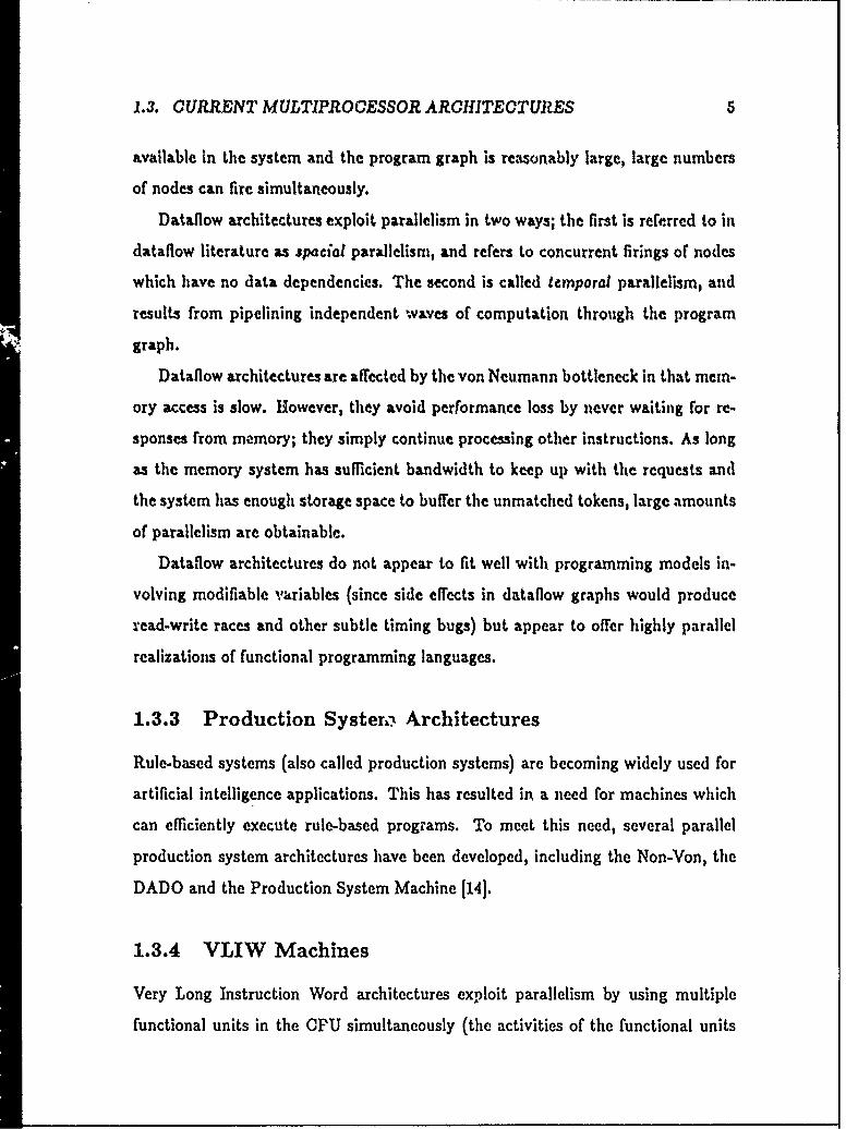
Dataflow architectures exploit parallelism in two ways; the first is referred to in

dataflow literature as spacial parallelism, and refers to concurrent firings of nodes

which have no data dependencies. The second is called temporal parallelLim, and

results from pipelining independent waves of computation through the program

graph.

Dataflow architectures are affected by the von Neumann bottleneck in that mem-

ory access is slow. However, they avoid performance loss by never waiting for re-

sponses from memory; they simply continue processing other instructions. As long

as the memory system has sufficient bandwidth to keep up with the requests and

the system has enough storage space to buffer the unmatched tokens, large amounts

of parallelism are obtainable.

Dataflow architectures do not appear to fit well with programming models in-

volving modifiable variables (since side effects in dataflow graphs would produce

read-write races and other subtle timing bugs) but appear to offer highly parallel

realizatioms of functional programming languages.

1.3.3 Production Systerz Architectures

Rule-based systems (also called production systems) are becoming widely used for

artificial intelligence applications. This has resulted in a need for machines which

can efficiently execute rule-based programs. To meet this need, several parallel

production system architectures have been developed, including the Non-Von, the

DADO and the Production System Machine [14].

1.3.4 VLIW Machines

Very Long Instruction Word architectures exploit parallelism by using multiple

functional units in the CPU simultaneously (the activities of the functional units

6 CHAPTER I. INTPODUCTION

are determined at compile time). Instruction words in a VLIW machine can be

hundreds of bits long, Though early experiments suggested that only a limited

amount of functional-unit parallelism was available, more recent work has shown

otherwise (22).

1.3.5 Pipelined Computers

Pipelining is a common technique for improving the performance of computers, and

can be combined with other techniques such as VLIW for obtaining large amounts

of parallelism. Pipelined functional units break up a function into a sequence of

small tasks which is carried out by pieces of hardware separated by registers. Each

task is designed to complete within one clock cycle, therefore every clock cycle an

intermediate result is passed from the output of a pipeline stage to the input of

the next stage. A new input can be given to the functional unit every cycle, The

throughput of a pipelined functional unit is a factor of s greater than the throughput

of the non-pipelined unit, where j is the latency of the non-pipelined unit divided

by the latency of one stage of the pipelined version. In very high-performance

architectures, memory is often pipelined as well.

1.3.6 Conventional MIMD Architectures

M.iMD architectures are those in which multiple conventional processing elements

operate independently. The processors coordinate their work either by sharing

memory locations or by sending messages to each other using special hardware

facilities.

This category can be further divided; all MIMD machines use multiple processor

elements and multiple memory elements but they can be connected in many different

ways. Several different MIMD machine organizations will be discussed in chapter 3.

MIMD architectures offer easier reuse of existing code than the other architec-

tures discussed here. If a MIMD machine has only a few processing elements, then

1.4. FOCUS OF THIS THESIS 7

conventional compilers can be used, and parallelism can be exploited at the user

process level. For more parallelism, compiler techniques such as trace scheduling

can help identify code fragments in a program that can bc overlapped. These tech-

niques can offer speedups of up to a factor of 90 (22). Finally, the programming

languages can be augmented with simple parallel constructs such as fork and join,

parallel do or futures 1151. Proper use of these constructs can reveal a great deal

of parallelism (depending on the application), particularly if the programmer keeps

parallelism in mind while writing the application.

1.4 Focus of This Thesis

This thesis is written in conjunction with the L project at the Computer Archi-

tecture Group, at MIT. £ is a model of computation, which means that it is an

abstract way of specifying how a program runs (where instructions come from, how

they are carried out, etc). For reasons discussed in the following chapter, L is more

suitable than the von Neumann model for describing multithread computations.

The L computation model assumes that tasks will be small to medium-grained

and does not commit to a technology for finding parallelism in programs. It assumes

that the parallelism has already been found; instructions for creating new threads of

control are explicit in the machine code. (For concreteness, this thesis will assume

that parallelism is generated from Multilisp-style futures, though in fact any of the

MIMD synchronization mechanisms mentioned above could be used.)

The object of this thesis is to present a highly scalable architecture for executing

L programs, i.e. an architecture that executes £ programs with speedup roughly

propor 'Onal to the number of processing elements in the system (given a sufficient

number of threads of control in the £ program). The proposed architecture falls into

the MIMD class, and uses a novel addressing technique called Cartesian Network-

Relative Addressing (CNRA).

8 CHAPTER 1. INTRODUCTION

Chapter 2

The L Project

The interface between programming langLes and mu'iprocessor hardware has

traditionally been based on the von Neumann assumptions of contiguous, homo-

geneous memories, bounded-size address spaces, and a single-sequence model of

program execution. The £ project is an effort to replace the von Neumann model

of computation with one which is better suited to modern programming languages

and modern multiprocessor hardware.

2.1 Chunks

The fundamental unit of storage in Z is the chunk, a fixed-size block composed

of nine 33-bit slots. Chunk slots in L replace the notion of memory locations in a

conventic nal computer. Each slot of a chunk may contain either a 32-bit scalar value

or a 32-bit reference to another chunk. The additional bit in each chunk is used to

distinguish between scalar and reference slots. This bit is called the reference bit

and its validity is maintained by the lowest-level execution model.

The first eight slots of each chunk contain data. The ninth slot of each chunk

is reserved to contain information about the type of the object represented by the

rest of the chunk, and is referred to as the type slot. The type slot can contain

10 OIIAPTER 2. TIHE . PROJECT

either sca-ar values or chunk references. Certain scalar values in the type slot arc

used to specify certain built-in chunk types (the remainder can be used by compiler-

enforced conventions), and references in the type slot may refer to type templates,

i.e. data structures that describe compound types.

All objects in L are implemented with chunks. Chunks naturally implement

small structures and small arrays. Larger structures can be built up out of U'ees of

chunks.

2.2 Chunk Identifiers

A facility for allocating chunks must be built into an Z runtime system, since there

may not be a contiguous memory at the bottom level on top of which a chunk

allocator can be written. When the runtime system allocates a chunk, it must

return a 32-bit chunk identifier (CID) which is a reference to the new chunk.

The CID abstraction must not be violated in an Z system. (The CiD abstraction

can be enforced by hardware or by compiler convention.) It must not be possible

for a program to manufacture a CID; only the chunk allocator should be able to do

this. (For debugging purposes it may be possible to convert cirs to integers.)

Throughout this thesis, the term "pointer" will be used interchangeably with

CID, chunk-ID, etc.

2.3 State Chunks

The state of an f processor has a standard representation which fits intc a single

chunk. Chunks containing processor state information are called STATE chunks and

are identified by a special scalar value in the type slot. For every thread of control

in an L system, there is a corresponding STATE chunk. Since STATE chunks are

identified by CIDS in the same way as all other chunks, they can be manipulated

using ordinary chunk-accessing operations; no complicated system-call mechanism

2.4. COMPUTATION IN P _1

L MacNne Code

Ro ln 1623

eisets 24-31 -Copy data koi om Wo io w-,oftrCre.le* stae chunks

Figure 2-1: An Active State Chunk

is needed. The concept of STATE chunks makes it easy to implement programming

models in which computation states are first-class data objects.

By compiler convention, several additional chunks may be allocated for each

STATE chunk, for use as temporary storage. These are called REGISTER chunks and

-4 accessible via chunk references in the STATE chunk (see Figure 2-1).

2.4 Computation in L

An 1 program is a set of chunks, some of which are STATE chunks, some of which

are DATA chunks and some of which are CODE chunks. To advance a computation,

the processing element selects a runnable state chunk to be advanced. The selected

12 CHAPTER 2. THE L PROJECT

state chunk is then advanced by executing the instruction pointed to by its code

pointer and offset, and then updating the code pointer and offset to point to the

next instruction. In a multiple-processor system, many STATES may be advanced

simultaneously. Note that the advancement of any STATE may lead to multiple

successor STATE3 (there are instructions in the instruction set that are akin to the

fork operation found in conventional operating systems).

2.5 Synchronization

Synchronization in Z is accomplished through a low level locking mechanism. Each

chunk has associated with it a locked" bit. Certain Z instructions block when

invoked on a locked chunk; threads of control that execute these instructions and

block will not be advanced until the locked chunk is unlocked.

2.6 L is a Practical Program/Machine Interface

There are many advantages to the use of Z as an interface between parallel al-

gorithms and parallel machines. Parallelism can be obtained any of a number of

different ways, compiled into an £ network and executed on the same computation

engine. £ only commits to a style of parallelism in that it is not well suited to very

fine-grained computation.

The fact that L dispenses with large address spaces in favour of chunks means

that £ networks can run on a variety of machines. An Z network can be run on

a large machine with a global address space (using a queue for runnable STATE

chunks) or can be run on a fine-grained SIMD machine by storing a chunk on each

node and performing associative lookups.

L supports just enough tagging to make garbage collection simple and to make

references easily identifiable to low-level processes that need to know the conse-

quences of re!ocating a chunk.

2.7. RISC AND THE DISTANCE METRIC ARGUMENT 13

The Z concept of tiny address spaces connected together means that the max-

imum size of an L network is not necessarily bounded depending on the size of an

address. Addresses (Z2 references) can be reused if the underlying storage manager

can keep the contexts straight. (This is, in fact, the main property of £ that is

exploited by the architecture proposed in this thesis.)

2.7 RISC And The Distance Metric Argument

A final advantage of £ as an interface reflects an architectural tenet that is described

in the next chapter of this thesis. That chapter contains an argument that uniform,

equidistant models of memory (sometimes referred to as paracomputer models 1241)

inhibit the sc.lability of an architecture. However, if an architecture attempts to

remedy this problem by using any type of non-uniform memory model, it is not

obvious whether this non-uniformity can be made evident to the programmer or

compiler without sacrificing generality of the computation model.

£ suggests a solution to this problem in the use of bounded-size objects and

tagged pointers. The number of pointer indirections from one object to a second

object can be used as a rough approximation of the computational expense of ac-

cessing the second object given the cm of the first object. This is a distance metric

that can be exploited both by compilers in their generation of £ code and by low-

level storage management facilities. Programs can assume that an object that is

fewer pointer indirections away than another is closer in the physical memory struc-

ture. The low-level memory management facilities can attempt to relocate objects

to minimize the "length" of pointers and thus minimize communication. (This is

straightforward because pointers are tagged.) This distance metric of number of

pointer indirections is completely architecture-independent.

It is fundamental to the RISC philosophy that as much of an architecture as

possible should be visible to compilers, in order to permit global optimization of

14 CHAPTER 2. THE Z, PROJECT

resource usage. The £ distance metric follows this philosophy by exposing "distance

in the memory system" to the compiler in an architecture-independent manner.

2.8 A Parallel Architecture For L

While Z is designed to be an efficient interface between many contemporary pro-

gramming languages and architectures, a particular architecture is proposed in the

remainder of this thesis, that exploits features of £ together with a novel technique

for managing address space to attain a high degree of scalability.

Chapter 3

Physical Space and Network

Topology

The backbone of a multiprocessor architecture is its communication substrate. Hlow

should the processor elements and memory elements be connected together?

There are many popular interconnection strategies.

* Small-scale multiprocessors (up to 32 processors or so) are often connected

with all processor and memory elements on a single bus. Bus traffic is reduced

by placing a cache between each processing element and the bus. Various

protocols (in which all caches "snoop" on the bus for transactions of interest)

are used to maintain cache consistency [11]. These systems provide a model of

memory in which all memory accesses take approximately the same amount

of time; all memory locations are "equidistant". Some examples of these

systems are the Alliant FX series, the ELXSI 6400, the Encore Multimax and

the Sequent Balance [8].

* Larger-scale multiprocessor that attempt to maintain an equidistant model of

memory have a characteristic structure of a set of processors on one side of an

interconnection network and a set of memory elements on the other side, and

15

16 CHAPTER 3. PHYSICAL SPACE AND NETWORK TOPOLOGY

have therefore been dubbed 'dance-hall" architectures [26). Some examples

of these systems are the BBN Butterfly (41, the IBM RP3 (231 and the NYU

Ultracomputer [131.

Other topologies do not attempt to provide an equidistant memory model.

They have processor elements and memory elements distributed among the

network nodes. Communications from one node to another are routed through

the network and travel different distances, depending on the locations in the

network of the sender and the receiver. Many of these systems have a boolean

n-cube topology, for example the Intel iPSC/2, the Floating Point Systems

T-series, the Ncube Ncube/10 [81 and the Caltech Cosmic Cube 1251.

3.1 The Case for Three-Dimensional Interconnect

If an important objective of an architecture is scalability, then the interconnect

topology of that architecture should appear to be connected in three or fewer di-

mensions. To state this more precisely, we must define a term that is like the fA

(big omega) notation but is slightly stronger. The usual definition of f) is as follows:

Definition 3-1:

A function T(n) is fl(g(n)) if there exists a positive constant c such that T(n) >

cg(n) infinitely often (for an infinite number of values of n) [1].

We define J to be a slightly stronger, perhaps slightly more intuitive term than f0:

Definition 3-2:

A function T(n) is J(g(n)) if there exists a positive constant c such that T(n) >

cg(n) for all but a finite number of values of n.

3.1. TIE CASE FOR ThIREE-DIMENSIONAL INTERCONNECT 17

Now we restate our maxim for scalable interconnect topologies: if n is the number of

nodes in a system and M(n) is the maximum number of nodes travelled by a message

in a system of size n, then M(n) must be J (. qn. (This rules out interconnection

topologies in which M(n) is J (log n), since log n increases more slowly than ./ .)

There are two arguments for this rule; one based on scalability considerations,

and one based on network performance considerations.

The Fundamental Constraint of Space

Let C(n) be the worst-case internode communication time in a system of n nodes.

First, we show that C(n) is J (-/ii). Therefore, if in any system M(n) increases at

a slower rate than V/n-, the internode communication time must increase with the

number of processors for systems larger than some size. Intuitively, this means that

if any network seems to offer logarithmic degradation of worst-case communication

with system size, that network will not scale.

Theorem: For any computer network with n nodes, where nodes have a physical

volume bounded below by v > 0 and have no physical dimension longer than p, the

worst-case one-way communication time from one node to another is J ('i.

Proof: The physical volume of the entire system is bounded below by Vn. The

shape with the smallest "maximal diameter" for a given volume is the sphere.

Consider a sphere with volume vn. The diameter of this sphere is given by:

r 3= vn

Thus the maximum physical distance from one point in the computer network to

another is bounded below by:

= vn-6/7r


where k is some positive constant. If one considers a communication between the

two nodes corresponding to these points, the physical distance travelled by the

communication is bounded below by:

kr/ -2p

(This distance is the minimum diameter of the system, minus twice the longest

dimension of a node.) The Lime for the worst-case one-way communication in the

system is therefore bounded below by:

krn - 2p

C

where c is the speed of light. Therefore:

C~n) >_ k, -q)k2

where k, and k2 are two positive constants. Now choose j such that 0 < j < ki.

We now have:C(n) >: j (n for all n > ( k

therefore C(n) is J(, /.

Network Performance Arguments For Low-Dimensional Net-

works

For a given wiring density in a multiprocessor, low dimensional networks per-

form better than high dimensional networks because the latter require a lot of

wiring space to interconnect, and that space that can be better used (in !o..di-

mensional networks) to increase the bandwidth of node-to-node connections [6].

Low-dimensional networks also have better hot-spot performance (because there

is more resource sharing) and can benefit more from increases in communication

locality.

3.2. OTIER FACTORS IN SELECTING A NETWORK 19

3.2 Other Factors in Selecting a Network

Homogeneity

Homogeneity is the property that there are no preferred locations in the system; all

processor/memory nodes in the system look "pretty much the samer [17]. This is

a useful property in a network for a multiprocessor, because it eliminates the need

to perform complicated optimizations in deciding how to position tasks and data

about the system. The positioning decisions can be based aolcly on (fundamental)

locality and concurrency constraints, and need not account for variations in node

capabilities.

Isotropy

Isotropy is the property that there are no preferred directions in the system; from

a given processor/memory node, the system looks "the same in all directions" [17).

This property is useful for exactly the same reasons as the homogeneity property; it

simplifies the decision-making process for placing tasks and data about the system.

3.3 The Three Dimensional Cartesian Hypertorus

The three-dimensional Cartesian hypertorus is a three-dimensional grid with the

boundaries connected. This topology is a logical choice in light of the previous

discussion.

First, by a simple extension of the argument given in section 3.1, the three-di-

mensional Cartesian hypertorus can emulate any other network to within a constant

factor of performance. (It is straightforward to show that the Cartesian hypertorus

can have 0(n) = k¢/i', and by the earlier argument, all networks must have C(n) >

k3 nii. Clearly the Cartesian hypertorus is never worse than a factor of k/ks slower

than another network.)

20 CHAPTER 3. PHYSICAL SPACE AND NETW([" TOPOLOGY

Figue P Ai T

Figure 3-1: A One-Dimensional Torus With a Long Wire

Figure 3-2: A One-Dimensional Torus With No Long Wires

,%eiond, the Carttsian hypertorus is homogeneous and isotropic. Th!vi, it can

be construcd without using any long wires. To illustrate how to connect up the

hyp :!oktus withont long wires, first consider a one-dimensional torus network (see

Figure 3d1). To eihain te lon- -ivies, half of the nodes can be moved onto the kti.g

,v*ze (see Figure 3-2). A two-dimer.imnal version (with some long wires) can now be

made by taking s'rveral one-dirnensional tori and connecting corresponding nod".

to each other. Initially, the end-around connection can be made with a long wire

(see Fir mr 3-3). Finally, half of the one-dimensional torus structures can be moved

over to the long wire (see Figure 3-4). This wiring trick can be extended to three

dimensions, though it has to be built correctly right from the start (one cannot take

two-dimensional tori and "slide them around" to the other side).

3.4 The Three Dimensional Cartesian Mesh

A second interconnection topology worthy of consideration is the (open) three-

dimensional Cartesian mesh. Though the Cartesian mesh has some disadvantages

over the torus, these are compensated by other advantages.

For example, one disadvantage of the open mesh is that it has twice the network

diamleter of the hypertorus for a given number of nodes. However, because there

3.4. THE THREE DIMENSIONAL CARTESIAN MESH 21

CDE tiII~ ~ II I

• D,m g a ii

aiur a-:AToDmnioa ou ihSeLnWis

pII as

as as as aI

aI a a Ia am

Figure 3-4: A Two-Dimensional Torus With No Long Wires


are no end-around connections, there is twice the wiring space available for a given

system size. Therefore the node-to-node bandwidth is doubled over the torus. A

second disadvantage of the open mesh is the lack of homogeneity and isotropy at

the boundaries. In practice, this may not be a significant problem since the number

of non-isotropic nodes increases only with the surface area of the three-dimensional

mesh, while the number of isotropic nodes increases with the volume of the mesh.

As the system is scaled up, the proportion of non-isotropic nodes decreases.

The three-dimensional mesh has the further advantage that one can construct

a system with a number of nodes that is not equal to the cube of an integer. This

is a practical benefit from allowing the network boundaries not to be homogeneous

and isotropic.

In the end, both the three-dimensional Cartesian hypertorus and the open three-

dimensional Cartesian grid are reasonable choices for a network.

3.5 Communication Locality

We have arrived at two network choices with the reasoning that these two networks

are no worse than any other. But are they good choices? In other words, is there

any network at all, on the basis of which a practical, general, scalable multiprocessor

can be constructed?

The answer to this question depends on the way the entire machine will be

programmed, and on the behaviour of typical programs. A multiprocessor will scale

well only if short-range communications are used significantly more often than long-

range communications. If this is not true and processors initiate communications

of completely random lengths, then overall system performance will decrease as the

system grows in size (since the distance of the average communication will increase)

no matter what interconnection topology is used. If, on the other hand, program

objects can be arranged such that short communications are more frequent than long

3.5. COMMUNICATION LOCALITY 23

ones, then either of the two proposed topologies may form the basis of a scalable

system.

An attempt to characterize which program communication behaviours will allow

a multiprocessor system to scale can be found in [9). In that paper, communica-

tion patterns are characterized by the rate at which interprocessor communication

decreases with distance. The conclusion is that communication must fall off faster

than the fourth powet of distance for a machine to scale.

24 CHAPTER 3. PHYSICAL SPA CE AND NETWORK TOPOLOGY

Chapter 4

Address Space Management

After selecting a network Iopology, the next task is to create a basis for interpreting

communications from one node to another. A communication from one node to

another is really a patterns of bits, and nothing else. Therefore there must be

some conventions for the interpretation of communications if they are to serve any

purpose. Such conventions can be enforced at any of several different levels; in

the lowest-level execution mechanism (microcode in some systems), at the machine

instruction level or at the high-level language level. Without loss of generality, we

will assume that communication interpretation conventions will be enforced at the

machine instruction level.

In the Z machine language, there are two simple types of data; the scalar and the

reference. A long message that is received by some node can be interpreted under

many possible compiler or programmer conventions, but a datum when finally used

by the £ instruction-processing mechanism must either be used as a scalar value or

as a reference. There is already an obvious convention for how to interpret a pattern

of bits as a scalar value, but there are many possibilities for how to interpret a bit

pattern as a reference. The way in which this is done can affect the scalability of

an architecture.

25

26 CHAPTER 4. ADDRESS SPACE MANAGEMENT

4.1 Common Address Interpretation Schemes

4.1.1 Local Memory Model

In the local memory model, an address selects a memory location on the node from

which the address is interpreted. There is no sequence of bits that, when interpreted

by one processor, can refer to data on another processor. Thus only scalar messages

can be sent from one node to another; if addresses are sent they lose their meaning.

4.1.2 Global Memory Model

In the global memory model, every memory location in the system has a unique

system-wide address. Thus a given sequence of bits refers to the same location in

the entire system, no matter which node interprets the address.

4.1.3 Mixed Memory Models

Local and global addressing models can be combined in the following manner: if

a node issues an address whose scalar value lies in one range, that address will

refer to a local memory location that is inaccessible to all other nodes. If a node

issues an address whose scalar value lies in another range, that address will refer

to a global memory location that is accessible to all nodes (that global location is

accessed using the same address, no matter which node initiates the access).

This scheme is used by the IBM RP-3 [23,5]. The RP-3 has a movable partition

which, at one extreme setting, makes the entire machine behave as a local memory

machine, and which at the other extreme, makes the machine behave as a global

memory machine.

4.2. A FORMALISM FOR MODELLING MEMORY ORGANIZATIONS 27

4.2 A Formalism For Modelling Memory Organi-

zations

In order to facilitate discusssion about how to meet different goals using different

address interpretation mechanisms, a formalism is presented for describing the ad-

dressing models of multiprocessors. This formalism will be referred to as the Intex

formalism, as it will be ultimately based on two functions, one which defines how

addresses are interpreted by the storage manageri and another which defines the

function of all execution engines in the system (thus this is the INTerpret/EXecute

formalism).


4.2.1 Domains Used in The Intex Formalism

locations = {J., 1,12,...}

names = (0,1,2,..)

scalars = {0,1,2,...}

values = scalars U {.}

configurations = {(.,i),(i,,i),(i,, 2),...) vj E values

Each element in the locations set corresponds to a physical location in a multi-

processor, in which a piece of data could be stored. This includes RAM, registers,

locations on the surface of a disk platter, etc. There is one element in the loca-

tions set that represents the "invalid location"; this is the result of dereferencing an

invalid pointer, etc.

Locations are said to always contain values, which can either be scalars or ..

This represents the reality that a location in the computer really stores only a string

of bits; any meaning to the bits is assigned by conventions in the processing element

and/or the storage manager. (A location is said to contain . if it has never been

assigned any data, if it is undefined, or if it does not contain valid data for some

reason.)

Names are those strings of bits that the processing element can send to a storage

manager; they are the valid addresses usable in the system.

A configuration set represents the entire state of a multiprocessor. It is a map-

ping from locations to values.

For the remainder of this chapter, the convention will be used that all variables

called n (with or without subscripts) are taken to be drawn from the set of names,

unless otherwise specified. All variables called c are configurations, all variables

called I are locations and all variables called v are values.


4.2.2 Relations Defined on the Domains

At a given time, a name that is specified by a processing element to a storage man-

ager represents some location in the system. The location it represents can depend

on which location contained the thread of control that initiated the transaction. We

define an interpretation function I, which takes a name, a location and a system

configuration and returns as its result the location specified if a thread of control

in the given location issues the given name in the given system configuration. The

function I has type:

I : ( name, location, configuration) - location

(This function is the interpretation part of the Intex formalism.) We also define V,

a function that returns the value stored in a location in a given configuration:

V ( location, configuration ) - value

V(c) = v if (, v) Ec

4.2.3 Modelling a Global Memory

To model a global memory system, define the address interpretation function as

follows:

Vn, 1,c I(n, 1,c) = 1,

Note that the function I does not vary with I and c; thus no matter which node

issues the address and what state the system is in, a given name always refers to

the same location. Note that this model precludes the use of forwarding pointers,1

since forwarding pointers change the location designated by some name (the name

IForwarding pointers are a mechanism that facilitates tasks such as garbage collection and objectmigration. A good example of their use can be found in the generational garbage collection algorithmof Lieberman and Hewitt 1211.


that formerly referred to the location where the forwarding pointer is stored, now

refers to the location where the forwarding pointer points). Also, this model does

not necessarily imply that each location has a unique name. (For example, one

could build a system with 4 Kbytes of memory which ignored the high 20 bitWs of

each address; thus address 0A34 would refer to the same location as address 1A34.)

4.2.4 Modelling a Local Memory

In a local memory model, any name issued from some node will be interpreted as a

location on that same node. Consider each node to contain m locations. Then one

possible address interpretation function is:

I(n, j, c) = m [-j + (ni mod in)

The idea is that one node contains locations lo to 1 m-1, another node contains

locations 1m to 12m-1, etc. If an address is interpreted from location ,'m then the

resulting location must be between 1,. and 12,-1. This is done by computing the

first node in this range (1m in this case) and adding the name, modulo the number

of elements on the node (this prevents accesses from "spilling over" onto the next

node).

4.2.5 Defining Some Properties of Naming Conventions

In this section, some properties of naming conventions will be defined, using the

relations defined in the previous sections.

Property 1: Time Invariance of Names.

Meaning: A given name from a given location will always refer to the same location.(The property we define is actually "configuration invariance of names", but sincea system changes configurations by executing instructions and performing garbagecollection, etc. the term "time invariance" seems more intuitive.)


Property 2: Location Invariance of Names.

Vn,lt,Li,c I(n,,,c) = I(n,l;,c)

Meaning: For a given -ystem configuration, a given name refers to the same locationno matter which location it is interpreted from.

Property 3: Name Constrains Location.

Vn 3L C locations such that V1, c I(n, 1, c) E L

Meaning: A given name inherently implies a set of possible locations; the namecannot refer to any location outside this set.

Property 4: Name Constrains Location, Relative.

Vn,l 3L C locations such that Vc I(n,1,c) E L

Meaning: A given name inherently implies a set of locations, but that set dependson its own location.

Property 5: All Locations Can Be Accessed From Any Location.

Vc, 1,,1i 3n I(n, 1,,c) = 1i

Property 6: All Locations Can be Accessed From Some Location.

Vc, 1i 3n,t 1j (n,t1jc) =tj

Property 7: Every Location Has a Unique Name For All Time.

V,n,, , , , li~ [(Ixni,l,c,) =0 1)A (I(;,,L;, ;) = t)] -, (n; = nj)

Property 8: Every Location Has a Unique Name At a Given Time.

VI,n,,ni, c, ,, i [(I(ni,i,,c)=)A(I(nlc) =)] -. (n = n)


Properties of a Global Shaid Memory Multiprocessor

A multiprocessor with a global shared memory and facilities for garbage collection

might have properties 1, 2, 3, 4 (follows from 3), 5 and 6 (follows from 5). The

machine may or may not have properties 7 or 8, depending on whether forwarding

pointers are supported by the low-level execution model. If they are, then forward-

ing pointers can be thought of as alternate names for a given location and thus the

properties do not hold.

4.2.6 A Simple Proof About These Properties

We would like to consider a multiprocessor that has no limitations on address space

but that has a finite number of names. The motivation for this comes from the

fact that it is easier to build an efficient processing element that uses fixed-length

addresses than it is to build one with variable-length addresses.

Theorem: If location invariance of names holds (property 2) and all locations can

be accessed from some location (property 6), then all locations can be accessed from

any location (property 5).

Proof: Consider a location 1. Since all locations can be accessed from some location,

let m be a location from which I can be accessed, and let n be a name with which

I can be accessed from m. Because of location invariance, the name n refers to

location 1, no matter which location uses the name. Therefore, I can be accessed

from any location.

Theorem: If Ilnamesl[ < Illocationsli then property 5 (all locations can be accessed

from any location) cannot hold.

Proof: This follows trivially from the fact that the number of locations that can

4.3. MODELLING THE EXECUTION OF PROGRAMS 33

be accessed from some given location is less than or equal to lnamesll.

Corollary: If I1namesil < Illocationsil then either property 2 or property 6 cannot

hold. This follows from the earlier proof that if property 2 and property 6 hold,

then property 5 holds.

As a practical aside, it is unreasonable to build a system with memory locations

that are completely inaccessible to all nodes. Thus property 6 should hold for

any system. From the corollary, it therefore seems that if the number of unique

addresses in the system is bounded and the number of accessible locations is not,

then a given name cannot always refer to the same object when used from different

locations.

4.3 Modelling the Execution of Programs

A program execution is modelled as a sequence of steps, each of which results

in the execution of an arbitrary number of instructions. The current state of a

computation is represented by:

" A system configuration as described earlier (a location-to-value mapping).

" A list of which locations currently designate active threads of control.

An execution step is defined as a function of two inputs (these inputs represent

the current state of the computation) which produces two outputs, representing the

new state of the computation. In a given step, any number of program instructions

can have been executed. The precise details of which instructions are executed

during a given step are left unspecified. Some systems may always execute a single

instruction (from a randomly-selected thread of control) for each time step. Other

systems may execute large numbers of instructions at each time step. Instructions


that execute at the same time step are considered semantically to have executed

simultaneously.

The execution function is defined as follows:

E =(C..,T.,) V

C,. and C., are system configurations. Ti- nd T.., are sets of locations that

represent the current set of runnable threads of control. (The E function is theVexecution engine" part of the Intex formalism.)

Without loss of generality, we state that the sole purpose of a program is to

compute a value.2 When the last execution step is performed on a computation

state, the result is the value v. This is the program's result value.

For convenience, we define the function E" (C, T) to denote che transitive closure

of E, i.e. the execution of zero or more steps.

We can now model a complete multiprocessor architecture by choosing a suitable

interpretation function I, execution function E, and starting system configuration

(C,T). The choice of E determines the overall model of computation, and the

choice of I determines the way in which addresses are managed in the system. The

choice of (C, T) determines the program that is to be run.

4.4 Transparency and "The Right Answer"

If a system starts in configuration (Cim,T,.) and

E' (C., IT,.) = v

Then we can say in some sense that v is the "right" answer resulting from the

execution of the program.

2 Really! This is a reasonable simplification because if we want to perform some computation forits vide tffect, we can model that in this system by following the computation with one which checksthat the side effect has taken place, and returns TRUE or FALSE as a result. If the side effect isnot detectible by another computation, I argue that it is a useless computation.

4.4. TRANSPARENCY AND "TIE RIGHT ANSWER" 35

In saying this, we are assuming that the instruction act supported by the E

function forces programs to be completely deterministic. (We are assuming there

is no input from the user, no generation of random numbers, etc.)

Let us examine the B function more closely. There are two types of functions

performed by the E function. The first of these functions is to select threads of

control to advance, and mechanically interpret their instructions. This is a direct

advancement of the computation. The second of these functions is to perform trans-

formations that reduce the number of execution steps required to run the program,

though they may not correspond directly with instructions represented in storage.

This is an indirect advancement of the computation. Examples of such transfor-

mations are garbage collection and relocation of data to improve communication

locality.

It would be nice to separate these two types of transformation so that our model

does not blur them together, but unfortunately there is no simple way to do this.

For example, if a multiprocessor system performs incremental garbage collection,

a given execution step (which corresponds vaguely to a time step) may perform

some GC actions and some processing actions. There is no way of defining an E

execution function and a G garbage collection function and talk about executing

an E step or a G step; this model would fail to capture the possibility of an access

conflicting with a garbage collection operation.

Indirect Transformations

Indirect computation advancements can be carried out in two ways.

1. They can be directly carried out by the E execution function (which can

perform a few types of transformation that it can promise will not disturb the

computation). Garbage collection is usually handled this way.


2. They can be carried out by the program that the B function is executing.

In other words, if an object must be moved somewhere, the program could

determine this by performing runtime computations, and executing instruc-

tions that would cause the object to be moved. Optimizations such as data

compression and compilation optimizations are often handled this way. In a

sense, these types of indirect transformation strongly resemble direct trans-

fcrmations (explicit program instructions are being carried out), but they

are slightly different; indirect transformations are intended to correspond to

optimizations that are not directly related to the executable program.

We will refer to these as "type 1" transformations and "type 2" transforma-

tions respectively. It is important not to conclude anything about efficiency when

considering which transformations are type 1 and which are type 2. In a real sys-

tem, the E function (the "execution engine") requires resources in proportion to its

functionality. Therefore, it will not necessarily improve system efficiency to ofload

work from the program code onto the execution engine.

Transparency and E as an Interface

We will characterize the difference between type 1 and type 2 transformations by

saying that type 1 transformations are transparent, and type 2 transformations are

not. A program can run without really being "aware" of a process if the process is

transparent.

The notion of transparency is not yet precise, since we have not yet defined

the E function in adequate detail. What are the instructions supported by the E

execution engine? It turns out that there are many details that must be decided:

, The instruction set could be considered to include high-level primitives, such

as the functions of the Unix standard I/O library - fopen, getchar, putchar,

4.4. TRANSPARENCY AND OTHE RIGHT ANSWER" 37

etc. If this were the case, then since the standard I/O library handles data

buffering, we might say that data buffering is handled transparently.

o The instruction set could be considered simply to be the machine language

interface of the processing element. (This would probably be a more natural

interface than one that included high-level language constructs.) In this case,

there may not be any transparent functions.

o Another option is whether or not the system has facilities for automatic

garbage collection. If so, it would be implemented in a transparent fashion

with the interface perhaps being the operating system system-call interface.

This analysis leads toward the following conclusions.

1. Transparency of operations involves conventions and guarantees. For example,

it may be that a system must require that memory be accessed only through a

predefined interface, in order to perform reliable garbage collection. Similarly

if a system can only access files via a standard I/O library, then file buffering

can be transparent. In reality, however, these are only conventions. At his or

*her own risk, a programmer can violate conventions (for example bypassing

stdio or malloc) and endanger the transparency of some operation.

For precision, we will say from now on that a process is considered transparent

with respect to a set of conventions. This means that if the conventions are

observed, the machine is guaranteed to compute the "right" answer.

2. A transparent transformation (with respect to some conventions) is consid-

ered correct if, when the conventions are followed and the transformation is

performed, the computation still returns the "right" answer.

Note that the more conventions we observe in the entire system, the more op-

timizations we can make transparently, but conventions are restrictive. The point


is to find the right balance. (These considerations are much of the motivation for

building RISC machines; designers began to realize that great benefit can some-

times be obtained by making transparent operations opaque. When the operations

are made opaque, it becomes possible to apply compiler optimizations, etc.)

4.5 L Conventions

L, as a model of computation, can be considered more restrictive than say, the

paracomputer model of computation. These restrictions are used in order to make

certain operations transparent (object migration for improving communication lo-

cality, determining which memory elements are accessible to which threads of con-

trol, and transparently adjusting pointers to implement sophisticated address space

models). Let us try to model the L conventions in the Intex formalism.

4.6 Modelling 1 In The Intex Formalism

£ is most naturally modelled by establishing a correspondence between Intex loca-

tions and £ chunks. (Another reasonably natural modelling is making the corre-

spondence between Intex locations and chunk slots, but this creates other difficul-

ties.)

4.6.1 Representation of Chunks

Since a chunk consists of 9 33-bit slots, a total of 297 bits is required to store the

contents of a chunk. We will therefore declare that the Intex scalar values can be

up to 297 bits long. Thus a location can store the entire contents of a chunk. The

contents of slot 0 are the 33 least significant bits of a chunk, the contents of slot 1

are the next 33 most significant bits, etc.

4.6. MODELLING ZC IN TIE INTEX FORMALISM 39

For notational convenience, define the ELT function as follows:

ELT(i, 3) = A ((2 3 1) < 33i)) > 33i 0 i < 8, E scalars

The function ELT(i, s) specifies the contents of the i&h slot of the chunk value s.

This representation of chunks and slot contents is slightly awkward. An alter-

native structure might be to make the model with each chunk slot corresponding

to a separate location. However, this idea introduces many more difficulties. For

example, we must require that (1) given the location of one slot of a chunk one

must be able to easily compute the locations of the other slots and (2) given a name

which, when used from some location refers to a slot of a chunk, one must be able

to easily compute names which will access the other slots.

4.6.2 Scalars And References

If the value stor.d in a slot of a chunk is greater than or equal to 212 it must be

treated as a reference, otherwise it must be treated as a scalar.

4.6.3 Chunk Allocation

There must be some convention that supports the existence of a chunk allocator in

the system. For example, the system could start up with a list of all the free locations

in the system stored in some known location. There could then be a globally

accessible interface from which a thread could obtain the name of a never-before-

allocated chunk. (That would make a poor implementation for a multiprocessor,

but that is not a concern right now. We are only concerned with what conventions

are required for a correct C implementation.)

3< and> are the left shift and right shift operators as used in the C programming language,and A is the logical bitwise "3nd" operator.


4.6.4 Meaning Of Stored Names

We will have to assign a semantics to stored names, independent of any usages

of those names by processing elements. If we did not assign a fixed meaning to

stored names, then a given chunk in memory could refer to one set of chunks when

accessed by one processor, and could refer to a second set of chunks when accessed

by a second processor, since the same stored bits could be interpreted differently

from the two different locations.

The meaning of the contents of a chunk should therefore not vary with the loca-

tion of the thread of control reading the chunk. This maxim might appear at first

to require location invariance of names in the system, but actually doesn't require

it. We can fulfill this maxim by defining the names in a chunk to be meaningful

when interpreted from the location of the chunk. More precisely, let:

' = ELT(i, v(l,c))

If s > 232 then it is a name that is intended to designate the location specified by

I(s,1, c).

4.7 Reachability

With the chunk semantics of , it is p' sible to define a concept of reachability;

this is the question of whether one chunk is accessible to another through a chain of

pointer indirections. This concept will be useful in discussing whether two or more

data accesses can conflict with each other.

We define the "Refs" property to be true if any slot of the chunk at location It

references the chunk at location li:

Refs (1jli,c) iff 3k 0 < k < 9 (ELT(k,V(I,,c)) > z)AI(ELT(k,V(,,c)),,,c) = Ii

I)eflne the uReachabled property to be true if the chunk at location Ii is accessible

4.8. TRANSPARENCY OF LOW-LEVEL OPERATIONS 41

by any number of indirections starting from the chunk at location 1j:

Reachable (1, Iic) iff ( Refs (1,, c)) V (31k Refs (I4 , k, c) A Reachable (1, c))

We now have a formal definition of reachability, based on the Z convention of how

to identify what bits in storage are intended to be names.

4.8 Transparency of Low-Level Operations

Under what circumstances can low-level operations such as garbage collection and

object migration be said to be "transparent"? When the value returned by the

computation remains the same, with or without the low-level operations. Let F be

an execution function that is just like E except that it performs some additional

low-level tasks such as garbage collection. F is a transparent extension of E if:

VC, T (' (C,T) = )A (F. (C,T) =,,,) -. (v = vi)

Under what circumstances can we promise that this is the case? How can we

guarantee that our transformations preserve program semantics? Again, it depends

on conventions. The more restrictive the conventions, the wider the class of trans-

formations we can make that are guaranteed to preserve program semantics.

Consider, for example, a model of a shared-memory globally addressed mul-

tiprocessor. With no conventions about how the E function behaves, there are

absolutely no transformations that can be guaranteed to preserve program seman-

tics. The program could read any random memory location at any time, and if

anything about the system is disturbed by a transformation that didn't correspond

to an instruction execution, the program could potentially return a different result.

What if, however, we had a conwation for locating the "free list" of unallocated

memory locations? (Assuming that the system used a memory allocator some-

where.) The E function could then remove locations from the free list and use

those locations for its own purposes. The range of things that the E function could


do would depend on what the guarantees of the memory allocation system were.

For example, if the conventions guaranteed that programs would never read or write

unallocated memory locations (something that is impossible to guarantee without

memory management facilities) then the E function could, for example, pop a loca-

tion from the free list, copy the contents of another location into this new location,

then change the name interpretation function so that (a) the name that referred to

the old location now refers to the new one, and (b) all names in the moved object

are adjusted if necessary, so that they are valid from their new location.

So we can now say that if there is a convention in the system that allows the

execution mechanism to safely identify and reserve unused memory locations, then

the execution mechanism can transparently move any object into an unallocated

memory location.

Garbage Collection

The process of transparent garbage collection can be thought of as (1) identifying

locations that are not on the free list, but that will never be used by the running

program, and (2) adding these locations to the free list. This is not possible in

the global memory system discussed above unless more conventions are adopted,

for determining which memory locations may be referenced. (These could include

conventions for identifying addresses in the program, conventions for determining

which instructions are read or write instructions, etc.)

The L conventions for determining reachability are enough to support the exis-

tence of a garbag(- collector, if one specifies that an £ thread of control only accesses

data that is reachable from the location designating the thread of control. For an

£ system in which the current computation is in state (C, {tI, t2 ,.. .}), the free list

should contain all chunks in

locations - ({ I Reachable (t 1,,C) } U {I I Reachable (t, 1, C) } U ...

4.9. DETERMINING THE EQUIVALENCE OF TWO NAMES 43

4.9 Determining The Equivalence of Two Names

It is important to know in a system whether the E interface can support a test to see

whether two names refer to the same location. There are many ways of approaching

this.

1. If property 7 holds (every location has a unique name for all time) or prop-

erty 8 holds (every location has a unique name at a given time), then the test

can be performed simply by comparing the two names. (If only property 8

holds, one must be careful that the comparison is made "instantaneously", i.e.

atomically. Otherwise, an object may change names during the comparison,

and a false result could occur.)

2. If neither of these properties holds, it may be that knowledge of the I function

for interpreting addresses can give insight into how to compute equivalence

of pointers. For example, if you know that I masks off the high bits of a

name and uses the result as a global address, then you can create a reliable

equivalence test by masking off the high bits for the test.

3. If none of the above techniques works, it is likely that a reliable, accurate

test for pointer equivalence cannot be computed. However, there may be a

partially complete equivalence test that sometimes returns a correct answer

and other times returns "don't know".

* If the two names are the same, they are definitely equivalent.

* If there is a convention for the instruction encodings that enables deter-

mination of the fact that the true/false answer is never used, then any

answer will do.


mination of the fact that the pointers being compared are never used,

then any answer will do.



mination of the fact that the pointers being compared are used for write

operations but never for read operations, then any answer will do.

There are dozens of special cases in which the true answer (to the pointer

equivalence test) may not be known, but special conventions allow the program

result to be computed anyway. In general, however, this is not good enough;

if a system supports a pointer comparison instruction, it must be able to

determine pointer equivalence reliably.

To sum up, if name equivalence is to be computable in a system, then either

there must be no name aliasing permitted, or knowledge about the behaviour of

the address interpretation function I must be exploited. In the latter case, name

equivalence may or may not be computable, depending on the details of T.

Chapter 5

Cartesian Network-Relative

Addressing

In the local addressing model, one address can refer to any of several different

memory locations, depending on which node issues the address. Assigning addresses

different meanings when interpreted from different nodes is essential if the amount

of address space is to scale with the number of nodes.

In the addressing convention described in this chapter, addresses are interpreted

relative to the node on which they reside, but any particular memory location can

be accessed from several nodes.

5.1 Introduction to CNRA

In the proposed scheme, addresses are composed of two components; a routi2g

component and a memory location component. The routing component represents

a displacement through the system's network, whose origin is the processor on which

the address resides. The memory location component is the memory location on

the node indicated by the displacement.

For an example, consider a system with a 9-bit routing component and a 23-bit

45

46 CIIAPTER 5. CARTESIAN NETWORK-RELATIVE ADDRESSING

Rlie~ tfspwwwm~tfrm ti curent node

x Y z

Figure 5-1: An Address In a ONRA Architecture

memory location component. Let the 9 routing bits be interpreted as three three-bit

values, each value representing a two's complement displacement along an axis in.

the network (see Figure 5-1). Now consider Figure 5-2. If processor A were to use

the address (-1,2,11, AE7F ), it would be specifying the data stored in memory

location AE7F on processor B.

This way of managing address space has many interesting properties, including

some of the advantages of global addressing models and some of the advantages

of local addressing models. Because addresses are interpreted relative to an origin

node, this system behaves like a local memory system in that the addition of each

new node introduces new address space into the system. However, because a given

memory location can be addressed by several nodes, you can have data sharing

similar to that used in global shared memory computers.

However, there are restrictions with this mechanism. The number of bits used

in the routing component of the address determines how far away in the network

something can be referenced. There is a difficult problem of how to manage this

non-uniform address space.

5.2 Some Definitions

In the discussion that follows, we will use the following terms:

5.2. SOME DEFINITIONS 47

B

N

- - A.7 .

X axis

Figure 5-2: Resolving An Address In a CNRA Architecture

Definition 5-1:

The addressing radius in a CNRA system is the maximum displacement along

any axis that can be specified with the routing bits. (In the examples above, the

addressing radius is three, since three bits can encode a displacement from -4 to +3

and we ignore the -4 for symmetry.)

Definition 5-2:

The addressing family of node N is the set of nodes that are within one addressing

radius of N.

48 CIIAPTER 5. CARTESIAN NETWORK-RELATIVE ADDRESSING

5.3 Computation in a CNRA System

An E computation in a CNRA system must initially be arranged (chunks assigned

to nodes) such that no chunk reference ever refers to a chunk further away than the

system's addressing radius. All mechanisms involved in executing an Z computation

maintain that invariant. (It can be made true at system startup by beginning the

entire computation on a single node, or by having the compiler initialize the system

to a consistent state.)

An f computation can be visualized as a three-dimensional 'cloud" of intercon-

nected chunk objects. The interconnections (chunk references) can be thought of

as pieces of string that connect slots of chunks to other chunks. The length of each

piece of string corresponds to the addressing radius of the system; no object can

contain a pointer to an object further than one string-length away.

Aside from this restriction on pointer length, computation proceeds in roughly

the same manner as it would on a globally-addressed system. (There are many

complications that arise from the limited-length pointers, but these will be discussed

in later chapters.)

5.4 Representing Large Structures

Since pointers are interpreted relative to the node on which they reside, data struc-

tures larger than the address space of a single processor can be represented. For

example, a long list could be represented by having the first m elements stored on

one node, with the mih list element pointing to the (m + 1)th list element on a

neighboring node. Some number of elements could be stored on that neighboring

node, with the last of those pointing one more node away, etc.

It is clear that an arbitrarily long list can be represented this way, though no

one processor can access all elements at a given time. In fact, if a task did try

to examine every element of a long list, it would eventually encounter an element

5.5. INCREASING CONCURRENCY AND LOAD BALANCING 49

whose next-element pointer pointed beyond its address space. At this point, the

storage manager would have to "tug on the list to pull the desired element into the

accessor's address space. This problem is discussed at greater length in chapter 6.

5.5 Increasing Concurrency And Load Balancing

In a CNRA systcm, there is no straightforward way to implement a global task

queue. State chunks must be distributed over the system, and must be executed

by processors near the nodes on which they reside. (The simplest system is to

have state chunks only be executed by the processing element at the node on which

they reside.) It is thus important for state chunks to be distributed over the entire

network as uniformly as possible. For computation models which support dynamic

creation of tasks, this means that there must be run-time support for load balancing.

Local Creation Of Tasks

One difficulty arising from the pointer-length restrictions in CNRA is that it a state

rhunk s, on node n initiates the creation of a new state chunk si, it will usually want

to initialize that new state chunk with some scalar values or chunk references. It

is possible, for example, that sj may want to initialize s with six chunk references,

each of which is a full addressing radius away in a different direction. In this case,

the most reasonable choice of node on which to create the new state chunk si is

node n, since if si were created on any other node, one of its initial references would

be too long, and some data structures in the system would have to be relocated

in order to make all chunk references satisfiable in s. (There are occasions in the

system when it is impossible to avoid moving data structures, but this is not one

of them.)

If state chunks are usually created on the node at which their parent resides, run-

time load balancing becomes even more important; it becomes the main mechanism

so CHAPTER 5. CARTESIAN NETWORK-RELATIVE ADDRESSING

for introducing concurrency into the system.

Transparent Load Balancing

Load balancing can be implemented in a transparent manner, by requiring that

STATB chunks have a tendency to move away from each other. (Protocols for achiev-

ing this effect are discussed an a later chapter.) If a state chunk contains a pointer

that is pointing as far away as possible in some direction, then that state chunk

cannot move in the opposite direction. All load balancing operations must respect

the "no pointer too long" invariant.

5.6 Decreasing Communication Requirements

Given static knowledge about the communication patterns in a program, a compiler

or programmer can initially arrange for tasks and data to be distributed about a

multiprocessor system to minimize communication costs. However, dynamic infor-

mation can also be exploited by monitoring data access patterns and relocating

objects to minimize communication.

The basic technique for implementing this type of object migration is to have an

attraction between each state chunk and the data accessed by that state chunk. This

attraction should increase slightly every time an access is performed, thus a state

chunk that accessed a variable in a tight inner loop would be much more attracted

to that variable than it would be to some other variable that it only accessed once.

5.7 The Tradeoff Between Locality And Concur-

rency

There is some tension between the requirements of increasing communication lo-

cality (reducing communication costs) and increasing concurrency. This tension is

5.7. THE TRADEOFF BETWEEN LOCALITY AND CONCURRENCY 51

fundamental in the concept of multiprocessing. The locality/concurrency tradeoff

is highly dependent on the details of the task (the ratio of computation to data

accessing, etc.). In the CNRA system, this tradeoff can be made by adjusting

the attraction and repulsion effects described above. Empirical study is needed to

determine which tradeoffs work best for which types of program.

It is worth noting that in programs with light communication requirements,

there is more opportunity for exploiting parallelism, and this is reflected in the"attraction/repulsionw effects described here. Furthermore, for programs with the

right characteristics, some threads may be able to migrate far beyond the address

spaces of other threads; in other words, full advantage may be taken of the unlimited

address space in the CNRA system. If, on the other hand, a program has very heavy

and 'fully connected" communication requirements, no state chunk will drift more

than an addressing radius away from any other state chunk, making the ONRA

system degrade gracefully to one with a 32-bit address space.

52 CHAPTER 6. CARTESIAN NETWORK-RELATIVE ADDRESSING

Chapter 6

Fundamental Issues in CNRA

Architectures

6.1 Forwarding Pointers

Some computers support forwarding pointers, a feature that enables two different

addresses to be aliased to refer to the same memory location. The use of forwarding

pointers facilitates garbage collection and compaction of memory 1211, but compli-

cates (and sometimes renders impossible) the operation of determining whether two

pointers refer to the same object. In & CNRA system, the choice of whether or not

to support forwarding pointers has many ramifications.

The main impact of supporting forwarding pointers in ONRA systems is that

with the forwarding pointers, it is possible for references to point to objects on nodes

that are outside the addressing family of the node on which the pointer resides. This

is a significant point that affects many different aspects of ONRA system design.

Softening of Pointer Distance Constraints

Normally in a ONRA system, the movement of an object is constrained by references

to it. The object cannot migrate to a node that is not in the intersection of the

53

54 CHAPTER 6. FUNDAMENTAL ISSUES IN CNRA ARCHITECTURES

addressing families of the nodes containing references to the object. In a system with

forwarding pointers however, these constraints are not present, since a forwarding

pointer can be left at the old location of a moved object.

Accesses that must traverse several forwarding pointers will naturally tike much

longer to process than ordinary accesses. Howtver, such transactions are impossi-

ble without forwarding pointers. In a sense, forwarding pointers 'soften" the con-

straints created by references; rather than simply refusing to allow the system to

enter certain configurations, forwarding pointers allow the system to enter them,

but with a performance penalty. This gives the object migration algorithm increased

flexibility.

Most CNRA issues that will be discussed in this chapter are strongly influenced

by whether or not forwarding pointers are supported.

6.2 Object Tables

An alternative to the use of forwarding pointers for increasing object mobility is

the use of an object table. This is used in many object-oriented systems (such as

Smalltalk). In such systems, each time an address is used it is looked up in the

table. All accesses have one level of indirection.

In single-node systems, object tables can provide an efficient, easy way to move

objects; one simply updates the table entry. Unfortunately, the situation is more

complicated for the multiple processor case, and even more so in ONRA. Obviously

it is not possible to have a single global object table. Therefore, we assume that

each node would have its own object table. Some possible interpretations of this

are:

1. All pointers are indices into the local object table. The addresses that are

obtained from looking up an index in the object table are relative addresses

(with routing components and memory location components).

6.3. READ AND WRITE NAMELOCK 55

2. All pointers are indices into the local object table. The addresses that are

obtained from looking up an index in the object table have two components;

the usual routing component, and a second component that is either a local

memory location (if the routing component indicates a local object) or an

object table entry number (if the routing component specifies any node other

than this one). In this latter case, the object table entry number is to be used

to index the object table at the node selected by the routing component.

Method 1 has the problem that many object tables can contain references to a

given object. If the object moves, they all must be modified. Furthermore, if the

object must be moved across a node boundary, a large amount of computation may

be needed in order to ensure that pointers to all of the objects it referred to are

available in the local object table.

Method 2 is somewhat better. An object can be moved by updating the local

object table to point to the new location, and (possibly) allocating an object table

entry in the new location. Unfortunately, this method means that looking up a

remote name may involve indirecting through several object tables; this technique

does not seem to offer any advantage over forwarding pointers.

Both methods involve a fair amount of complication if a thread copies a pointer

into an object on another node. It really seems that object tables are more trouble

than they are worth in the context of CNRA multiprocessors.

6.3 Read And Write Nanielock

It is not obvious how to handle remote requests involving names. The difficulty is

that stored names are considered to be valid when interpreted from the node on

which they reside. Therefore, if a neighboring node reads the name, the name must

be adjusted as the neighbor receives it. For example, if a thread of control on node

n reads a name from the node one to its north, and the name was stored as (1,


0, 2, 3AEO), the thread of control should actually "see" the name (2, 0, 2, 3AEO).

This way, if the thread of control uses the name, it will refer to the object that was

referred to by the stored name. Similarly, if a thread of control writes a name to

memory, the name should be adjusted so that it is valid from its stored location.

There are two problems that can arise from this, one from write operations and

one from read operations. The write problem (which we will call "write namelock")

will occur when a thread of control attempts to write some name to some location,

and the object referred to by the name is outside the location's addressing family.

"Read namelock" occurs when a thread of control in some location reads some

name, and the name refers to an object outside the location's addressing family. In

both of these situations, the adjustment that needs to be made to the name cannot

be made because of addressing radius limitations. There are two solutions to the

namelock problem, depending on whether or not the system supports forwarding

pointers.

Solving Namelock With Forwarding Pointers

Tf the system does support forwarding pointers, the solution is simply to create

one when namelock occurs. For both read and write namelock, it is guaranteed

that only one forwarding pointer will be needed. (In read namelock, the forwarding

pointer can be stored on the node of the name that is being read; the name can

clearly be valid from that node, and that node is clearly in the addressing family of

the initiating thread of control. In write namelock, the forwarding pointer can be

stored on the node of the initiating thread of control; the name can clearly be valid

from that node, and that node must be accessible to the destination node of the

write operation. Note that this last statement is only true if the addressing family

of any node is symmetrical about the node.)

6.4, TESTING POINTERS FOR EQUIVALENCE 57

Solving Namelock Without Forwarding Pointers

If the CNRA system does not support forwarding pointers, there is no simple way

out of the namelock situation. The read or write operation simply cannot complete

with the objects in the po6itions that they are. The solution must therefore be

to make the object migrator act on (a) the object whose address is being read or

written and on (b) the thread of control object initiating the transaction, so that

they are forced to migrate toward each other with the highest possible priority. The

namelock simply cannot be resolved until the objects involved become closer in the

network.

In the worst case, both the thread and data objects could be fully constrained

by references so that they could not move toward each other. In this case, the

high-priority migration instructions must propagate through the object network,

causing as many objects as are necessary to move until the system can reach a

configuration in which the two namelocked objects are brought together. It is

unlikely that pathological cases will occur often if the addressing radius of the

system is reasonably generous. On the other hand, systems with large addressing

radii have the disadvantage that namelocks can be more severe; in a system with

addressing radius r, each object that is moved to resolve a namelock might have to

be moved as many as r nodes.

This problem of namelock is the most compelling argument for forwarding point-

ers; though forwarding pointers add many complications to the CNRA system over-

all, they offer a much more "gentle" solution to the namelock problem.

6.4 Testing Pointers for Equivalence

The computability of whether or not, two pointers refer to the same object depends

on whether the system supports forwarding pointers or object tables. Obviously

if the system supports neither, pointer equivalence is simple to compute; the two


pointers can simply be tested for bit-for-bit equality. If the system uses object tables,

the test for pointer equivalence depends heavily on the object table management

strategies. Since object tables do not seem to be useful in a CNRA setting, we will

not discuss solutions to that case.

In systems that do support forwarding pointers, one cannot always determine

the equivalence of two pointers by comparing their values; if they are equal in value,

then they are certainly equivalent, but if they are not equal in value, no conclusions

can be drawn.

In the latter case, the pointer equivalence test can be performed by computing

canonical representations of the objects' actual locations (relative to the requestor),

then comparing the canonical representations to see if they are identical. This solu-

tion requires that (1) there be a canonical representation for any location (relative

to any other location), and that (2) there be some way of guaranteeing that objects

do not migrate during the test in a fashion that could cause an incorrect result.

The first requirement is met by the fact that an (X, Y, Z) triple of arbitrary-

length integers can specify the location of any node relative to any other in a

canonical way. The following protocol for determining pointer equivalence also

meets the second requirement:

1. Send an "equivalence probe" request to the node designated by the first

pointer. Normally, any request that involves a pointer (even just "read" or"write") must accumulate its total X, Y and Z displacement as it travels to

its destination, so that the result can be returned to the requestor. For an

equivalence probe request, the X, Y and Z displacements that enable com-

putation of the return path are also the result of the request. (The result

also contains the memory location of the destination object.) The equivalence

probe thus returns a canonical representation of the location of the pointed-to

object, relative to the requestor. As a side effect, the equivalence probe must

"freeze" the object that was probed; that object should no longer be garbage

6.5. OBJECT MIGRATION 59

collected or migrated.

2. Send an "equivalence probe" to the second object as well.

3. Compare the results of the two probes. If the results are identical, the original

pointers were equivalent. If the results are different, the pointers were not

equivalent.

4. Finally, now that the result has been computed, s(nd an "unfreeze object"

request to the object(s) referred to by the two original pointers.

6.5 Object Migration

Object migration plays a very important role in the ONRA architecture. In a

conventional system where all objects can be globally addressed, problems of task

and data distribution over the system can be handled by global mechanisms (i.e.Uwhen a processor is free, it should pop a task from the global task queue and assume

responsibility for completing that task"). However, in a CNRA system many nodes

are inaccessible to a given node; tasks can only spread onto other nodes, the way a

puddle of water might spread across a fiat surface.

In general, achieving some system-wide characteristic in a running CNRA sys-

tem requires that individual nodes implement local rules that produce the global

effect when followed all together. This means that it is worth putting an immense

amount of effort into making node-to-neighboring-node communications extremely

inexpensive, so that if a command must "ripple" through the network, the total

amount of time taken is not excessive.

The migration mechanism for increasing parallelism (load balancing) must take

some account of the processing elements' speed and of the typical grain of program

parallelism. This information can be used to ensure that the average time between

migrations is significantly shorter than the average lifetime of a program thread


of control. (This is necessary if the migration is to be of much use in improving

communication locality.)

6.5.1 Migration With Forwarding Pointers

If a CNRA system supports forwarding pointers, the algorithm for relocating an

object is straightforward. One simply needs to copy the object to the new location

(adjusting internal pointers if necessary) then leave a forwarding pointer at the old

location of the object. If any of the object's internal pointers were already fully

extended, then the migration system could either decide not to move the object, or

could create some additional forwarding pointers through which the moved object

could continue to follow old references. Forwarding pointers in the system could be

removed by the garbage collection process.

6.5.2 Migration By the Garbage Collector

If a CNRA system does not support forwarding pointers, then migrating objects

is more difficult. One possible solution is to make the garbage collector the only

mechanism that moves objects. If the migration mechanism decides that an object

should move to some particular node, it can leave a message to that effect in the

object, and when the garbage collector next touches the object, it can arrange for

the move. The garbage collector would have access to all of the objects pointing to

the object to be moved, and would therefore be able to adjust their references to

point to the new location.

In this system, garbage collection would have to be performed very frequently,

since objects should get several chances to move during the average lifetime of a

thread of control. This means that the performance of the garbage collector would

probably benefit greatly from generational garbage collection techniques [211.

A garbage collector that can handle object migration is described in Section 7.8.1.

6.6. GARBAGE COLLECTION 61

6.5.3 Migration With Incoming-Reference Lists

A final alternative to the use of forwarding pointers or garbage collection for object

migration would be for each object to keep a list of which objects had pointers to

it. In this scheme, some bookkeeping would have to be performed for every write

operation that occurred. If the former contents of the newly-written location were

a pointer, then that pointer would have to be dereferenced to locate the pointed-

to object and the pointed-to-object's list of incoming references would have to be

adjusted (an element would be deleted). Then, if the newly stored value is also

a reference, that must be dereferenced and the pointed-to object must have its

incoming reference list adjusted (an element would be added).

Note that this scheme works reasonably well with CNRA constraints, since ele-

ments in an "incoming reference" list need never point further than one addressing

radius away. (They only have to point to objects which have references to them.)

This scheme, though probably computationally expensive to implement (there

could be up to two updates to incoming-reference lists for each write transaction),

makes object movement straightforward, since the references to any object can

immediately be identified. (A small amount of extra complexity would be needed

to make sure that a processor that had cached an object address didn't get out of

sync with the rest of the system.)

6.6 Garbage Collection

Garbage collection is a difficult problem for most multiprocessor architectures. Let

us consider various garbage collection techniques and see whether they can be

adapted to CNRA systems.


6.6.1 Reference Counting

Reference-counting garbage collectors associate with each object a count of the

number of references to that object. When that count reaches zero, the object is

inaccessible and the storage manager can reclaim its storage.

Reference counting can be implemented on a ONRA system in a straightforward

manner. When a pointer is copied, the reference count can be incremented (the very

fact that there is a reference means that the referencer and the referencee are within

an addressing radius of each other), and if a pointer is deleted, the reference counts

can be decremented in the same manner. When an object's storage is reclaimed,

the storage can be reused by the node on which the object last resided.

Reference counting suffers from the disadvantages of not being able to reclaim

cyclic structures, and of requiring one or two bookkeeping transactions for each

write operation. (However, this might combine nicely with the "incoming reference"

system described above for object migration; the length of the list of incoming

references is also the reference count.)

For systems with very large memories, reference counting is sometimes sufficient

for garbage collection ([101, p.6 76).

6.6.2 Mark/Sweep Garbage Collectors

Mark/sweep garbage collectors start at a root object (or set of objects) and mark

the graph of all objects accessible from the root set. Then all objects in memory

are scanned and those that were not marked are reclaimed. (The root set on a

conventional computer can be defined to be the task queue.)

Mark/sweep garbage collectors can reclaim circular structures, and do not re-

quire bookkeeping transactions during ordinary processor activity. However, it is

not obvious how to apply them to a CNRA multiprocessor. It is not feasible to per-

form a single mark/sweep collection over all memory in the system, since the r3ot

set of objects (all active tasks in the system) is distributed over the entire system,


and there is no straightforward way to sweep the entire memory.

A better approach would be to have each processor perform mark/sweep collec-

tions on its local memory. This could be implemented by having each node keep a

list of all reference to its objects from objects on other nodes. The mark/sweep col-

lection would then include in the root set all thread of control objects (i.e. the task

queue), and all objects listed in the external reference table. Reference counting

could be used for inter-node transactions, i.e. objects that were pointed to by remote

references would have reference counts that would be adjusted only when remote

references were created or deleted. Such objects, being listed in the local entry table

and therefore included in the root set, would never be garbage collected. When the

last remote reference was deleted, the object's address would be removed from the

entry table, and the object would again be subject to local garbage collection.

This system would have many of the advantages of a mark/sweep collector, but

would not be able to reclaim cyclic structures that spanned node boundaries. It

would still be better than a pure reference-counting garbage collector, though. A

final improvement could be to modify the object migration algorithm so that cycles

that spanned node boundaries tended to eventually coalesce onto a single processor.

This last improvement would allow multiple-node cyclic structures to be reclaimed,

as long as external reference tables were properly managed [16,17).

6.6.3 Final Comments On Garbage Collection

It is worth noting that none of these garbage collection algorithms inherently require

the ability to test pointer equivalence. Thus an architectural variation on CNRA

that precludes such tests should not necessarily be ruled out.

Also, we will not yet discuss the interactions between the issues described above.

Garbage collection, for example, may be considerably harder in the presence of

object migration and/or forwarding pointers. This will be discussed more in the

next chapter, which contains the foundation of a design for a CNRA machine.

64 CtAPTER 6. FUNDAMENTAL ISSUES IN CNRA ARCHITECTURES

6.7 Data Structure Representation Restrictions

The total amount of address space in a CNRA system is unbounded. However,

there are restrictions on the size of individual data structures in the system. These

restrictions depend on the fanout of the data structures.

Consider, for example, a linked list represented on a two-dimensional CNRA

system. An arbitrarily long list can be represented in the following manner. If m is

the maximum number of list elements that can be stored on a system node, store

th4 first m elements on one node, then store the next m elements on a neighboring

node, then the next m elements on the neighboring node continuing in the same

direction, etc. It is clear that an arbitrarily long list can be represented this way,

even on a system with an addressing radius of only 1.

Now, however, consider a binary tree represented on the same CNRA system.

The root node of the tree must be stored on some node n. Now say the tree has

depth 1. Since there must be references from the root to the children, the entire

tree must be stored within the addressing family of n. In a two-dimensional CNRA

system with an addressing radius of two, this would give a possible 25 nodes in

which the parts of the tree could reside (the addressing family includes nodes up to

two nodes away in any dimension from n, defining a 5 x 5 square).

Next, consider a binary tree of depth 2 on the same system. The parts of the

tree can be stored in any nodes in the addressing family of any of the 25 nodes for

the first two levels of the tree. This gives a total amount of storage corresponding

to a 9 x 9 square of nodes.

In general, the amount of available storage for a given structure in the two-

dimensional CNRA system with addressing radius r, is limited by

m(1 + 2dr)2

where m is the amount of available storage. at each node, and d is the depth of the

structure.

6.7. DATA STRUCTURE REPRESENTATION RESTRICTIONS 65

This Is quite significant, as the total available storage only increases with the

square of the depth of the structure. If the structure's size is exponential in its

depth, as is the case for any tree, of branching factor greater than or equal to two,

there will be some limit on its maximum depth.

In the case of a three dimensional CNRA system, the amount of available storage

is limited by

m(l + 2dr)3

where rn, d and r are defined as before. The available storage in this case increases

with the cube of the structure's depth.

To see how these limitations may impact programmers, consider Figure 6-1. This

figure shows, for a CNRA machine with 32-bit addresses, the maximum amount of

address space available for any one data structure, depending on the structure's

depth, and on the number of bits used for routing versus memory addressing. Fig-

ure 6-2 shows the same information for a machine with 16-bit addresses. In these

figures, the structure depth axis varies from 0 to 54 in increments of 6. The other

axis is the number of bits dedicated to routing. A value of z along the Z-axis means

that for that data point, z bits of address space are available for a given single data

structure (i.e. the structure must fit in 2' memory locations). The graphs assume

that the addressing families are cube-shaped (see Section 6.8).

For the 32-bit graph (Figure 6-1), note that the amount of address space seems

to level out at around 46 or 47 bits of address space. This means that a CNRA

system with 32-bit addresses cannot store a balanced binary tree of depth more

than 45 or 46.

Forwarding Pointers Remove Data Structure Limitations

Adding forwarding pointers to a ONRA system removes the data structure limita-

tions discussed above. The following proof shows that an arbitrary-depth tree of any

reasonable branching factor can be represented in a CNRA system with forwarding


so

'10

Figure 6-1: 3D ONRA System, 32-Bit Addressing: Address Space Per Structure


40

Figue 82: 3 ONA Ss~em 18BitAddrssig: ddres SacePer trutur

68 CIIAPTER 6. FUNDAMENTAL ISSUES IN CNRA ARCHIITECTURES

pointers.

Theorem: If each node in a two dimensional CNRA network has enough address

space (and storage) to store one tree node or n forwarding pointers, then the CNRA

network can represent any tree of branching factor n or less without running out of

address space. (The size of the tree will of course be limited by available memory.)

In the proof, I will use the term *element" to mean "tree node", and "node" to

mean "CNRA system node" to avoid ambiguity.

Proof: We will use a constructive proof, by induction on the depth of the tree. We

will note that the trees constructed in this proof have two important properties.

The first is that all constructed trees will fit in a rectangular array of nodes. The

second is that the root element of any constructed tree is always on the node at the

top left corner of the rectangle.

Basis step: A tree of depth zero can be stored on a single node. The two require-

ments that (1) the tree occupy a rectangle of nodes and (2) the root element is

stored on the top left node, are both met.

Induction step: Here is how to construct a tree of depth d + 1, given n trees of

depth d. (See Figure 6-3.) Place the n trees side by side. This "forest" occupies a

rectangular array of nodes, the same height as the individual rectangles that contain

the n original trees, and n times the width. On the node one higher and one to

the left of the top left node of this new rectangle, place the root element of the

new tree. Allocate n forwarding pointers on the node to the right of this new root

node. Set the children pointers of the root element to point to the n new forwarding

pointers. Of the n newly-created forwarding pointers, set the first to point to the

element one node immediately below. Now, on the node to the right of the one with

the n forwarding pointers, create (n - 1) more forwarding pointers. The (n - 1)


Forwarding pointars

YN -T -T N -I I I

Internai N N N Ntree nodes

Two trees of depth 1

Figure 6-3: The Second Induction Step For a Binary Tree

forwarding pointers that remain from the first group should be set to point to the

newly-created (n - 1) pointers. These newly-created, (n - 1) pointers should point

to (n - 1) more pointers on the next node to the right, and so on, until the point

above the root node of the next child. Thcn, again, one of the forwarding pointers

must continue down to point to the second child. The remaining (n - 2) pointers

must continue on to the right, etc. When this process is done, we have our tree. If

the width and height of the n original trees were w and h nodes respectively, then

the width and height of the new tree are (nw + 1) and (h + 1) nodes, respectively.

The new tree is rectangular, as required, and the root node is at the top left corner.

Obviously, if this construction works for a two-dimensional CNRA system w*,t tn

addressing radius of one and a ridiculously small amount of memory per node, then

it helds for any two or three-dimensional CNRA system!


6.8 Alternate Routing Schemes

Throughout this thesis, it has been assumed that the routing bits would be divided

into three parts (one for each dimension of the CNRA system) and each part would

be a two's complement representation of a displacement along an axis from the

node.

However, this representation is slightly awkward because of the asymmetry of

two's complement notation. The system must either allow the possibility of pointers

reaching farther in one direction than in another, or they must waste part of the

bitspace of the pointers.

There are alternative routing schemes which may be less intuitive, but may

make better use of the bit space. To see how well the bit space can be used, let

us consider various possible sizes of addressing families, and see how close we can

come to a power of two without going over. Table 6.1 shows all addressing family

sizes for addressing radii up to 200 that are within 5% of the next power of two, for

cube-shaped addressing families.

This table means that CNRA systems with one of the listed addressing radii

(2, 12, etc.) will have the most potential to use the routing bit-space efficiently. A

three-dimensional system with addressing radius 2, for example, has an addressing

family of size 125. This system could be built with 7 routing bits, and would waste

only 3 bit combinations. The mapping from the other bit combinations to nodes in

the addressing family can be arbitrary. (This may have the side effect of making

it hard to compute the new routing components for pointers that move, but for

systems with small addressing radii, that operation could be accomplished with a

lookup table.)

Note that (assuming a binary-based system) the number of bit combinations will

always be a power of two. (Any prime factorization of these numbers will always

contain only powers of two.) However, in any CNRA system, the addressing family

6.8. ALTERNATE ROUTING SCHEMES 71

Addressing Size of Addressing Next Higher Percentage of

Radius Family Power of Two Wasted Bitspace

2 125 128 2.3412 15,625 16,384 4.6331 250,047 26Y,144 4.6150 1,030,301 1,048,576 1.7463 2,048,383 2,097,152 2.3379 4,019,679 4,194,304 4.1680 4,173,281 4,194,304 0.50100 8,120,601 8,388,608 3.19101 8,365,427 81388,608 0.28126 16,194,277 16,777,216 3.47127 16,581,375 16,777,216 1.17159 32,461,759 33,554,432 3.26160 33,076,161 33,554,432 1.43200 64,4b±,201 67,108,864 3.92

Table 6.1: Cubic Addressing Family Sizes Close to Pows:s of Two

(assuming it is always symmetrical about a node) will always be a power of an

odd number, which means that there will always be at least one prime factor not

equal to two. Thus no addressing family can ever be precisely a power of two, and

therefore no CNRA syszem will ever use 100% of the available routing space.

Non-Cube Addressing Family Shapes

We have been assuming that addressing families are always cube-shaped, in other

words, if the addressing radius is two, then a reference can point to an object up to

two nodes away along any or all axes. Another reasonable definition of "addressing

radius of two" is that the addressing family includes all nodes that are two network

hops dissant or less. In a two dimensional system, for example, the addressing

families would be as shown in Figure 6-4.

Let us define f(n) to be the number of nodes in each addressing family of a

two-dimensional CNRA system with an addressing radius of n. For the system in


Addressing radius. 1- -- Addressing radius 2

% %J -f

% % I

Figure 6-4: CYRA System, Addressing Radius Is Maximum Manhattan Distance

which the addressing radius refers to the number of network hops, we have:

f (n) = 2n2 + 2n + 1

Define g(n) to have the same meaning as .f'(n), but for a three-dimensional CNRA

systems in which the addressing radius refers to the number of network hops. We

can define g(n) using a recursion, as follows:

g(0) = .f(0)n-I- n)- f(n) +-2,f(i) n>l

i=0

The idea of his recursion is to con ddressi adssng family of a node, on a system

in which the addressing radius is, say, 4. If you examine a two-dimensional slice of

the network containing that node, you would see f(4) accesible nodes. The slices

"oene go ave te below" this slice would each contain f(3) accessible nodes,

etc. The closed-form solution to this recursion is:

g() = + +

q~n)= fn-+2n:f-t-

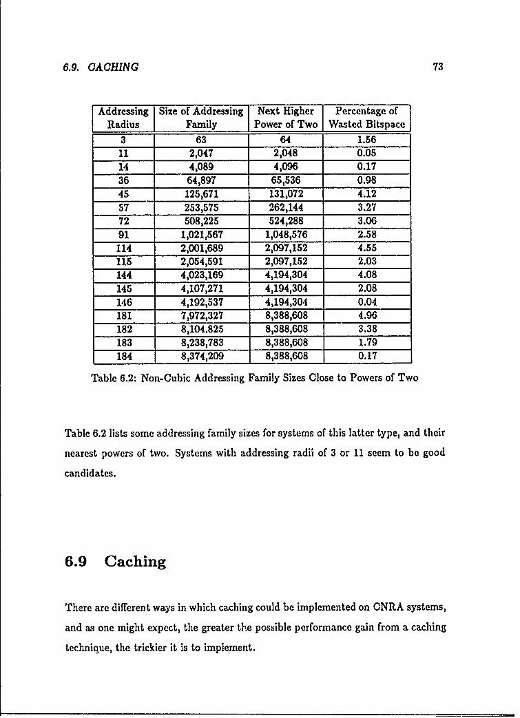
6.9. CACHING 73

Addressing Size of Addressing Next Higher Percentage ofRadius Family Power of Two Wasted Bitspace

3 63 64 1.5611 2,047 2,048 0.0514 4,089 4,096 0.1736 64,897 65,536 0.9845 125,671 131,072 4.1257 253,575 262,144 3.2772 508,225 524,288 3.0691 1,021,567 1,048,576 2.58

114 2,001,689 2,097,152 4.55115 2,054,591 2,097,152 2.03144 4,023,169 4,194,304 4.08145 4,107,271 4,194,304 2.08146 4,192,537 4,194,304 0.04181 7,972,327 8,388,608 4.96182 8,104.825 8,388,608 3.38183 8,238,783 8,388,608 1.79184 8,374,209 8,388,608 0.17

Table 6.2: Non-Cubic Addressing Family Sizes Close to Powers of Two

Table 6.2 lists some addressing family sizes for systems of this latter type, and their

nearest powers of two. Systems with addressing radii of 3 or 11 seem to be good

candidates.

6.9 Caching

There are different ways in which caching could be implemented on CNRA systems,

and as one might expect, the greater the possible performance gain from a caching

technique, the trickier it is to implement.


6.9.1 Local Caching Only

A simple technique that would improve performance over the vanilla CNRA system

would be to use a local cache at each node, that only cached data residing at that

node. So, for example, if everything were running on one node (and thus all refcr-

ences had the same routing compcnent) it would all be cached as in a conventional

computer. If an object migrated to a neighboring node however, its cache entry

would immediately be flushed. It might then be cached hi the neighboring node.

This caching scheme would not help remote accesses much, but if it turned out that

most accesses are local, then some performance improvement could be obtained.

6.9.2 Remote Caching, No Forwarding Pointers

If the CNRA system does not support forwarding pointers, there is a possibility

that each node could cache the results of all of its references. This would create

a cache consistency problem, since a given datum might reside in more than one

cache at a time. However, objects stored on a given node willi never be cached in

any processor outside of that node's addressing family, so if that addressing family

is reasonably small (perhaps 27 nodes), it is feasible for each node to snoop on the

bus transactions of all other nodes in its addressing family. This has the potential

to greatly increase system performance.

Chapter 7

Foundation For a CNRA Machine

Based on PC

An £ computation at a given point in thne is completely repiesented by a set of

-inter-referencing chunks. The computation is carried out by processing elements

%OILOI. OCA1v~ A UIIIAA J ~AI a w U 4S_ -*a- ... .d-net..-i. . ' .. . . ni

The initial design will thus be to have the multiprocessor built as a network of

memories that can represent an £ computation. Coupled with each memory will be

a processing element (PE) that will be "checkinge for runnable threads of control

(state chunks) on that memory. Whenever there are one or more active state chunks

on tha¢. memory module, the associated PE will keep advancing their computations.

(Another implementation technique might be to only use one processor element for

both computation and for storage management, perhaps switching between some

sort of supervisor and user modes. For now, we will assume that the processor

element and memory manager element are separate.)

The idea of having each processor only execute threads whose state cl.,nks reside

on its associated memory module has the virtue of simplicity. A more sophisticated

L implementation might involve lightly loaded processors hunting for work in the

memories of neighbors. For now, we will rely on the task migration mechanism to

75

76 CHAPTER 7. FOUNDATION FOR A CNRA MACHINE BASED ON £

explicitly move state chunks to distribute the work as much as possible. We would

need the task migration mechanism anyway, so we might as well start with only

that, then add more sophisticated work distribution strategies if necessary.

Given that a processing element has more than enough state chunks to keep

it busy, the algorithm for selecting which state chunks to run is unspecified. This

permits £ implementations, for example, to execute several instructions from a

given state chunk before selecting another state chunk if that is more efficient.

We will abbreviate "processing element" as PE and "memory controller" as MC.

The MC for each node will manage the flow of chunks to and from the node, make

it easy for the node's PE to identify runnable state chunks, and perform storage

management functions such as garbage collection.

7.1 Basic Structure

For the three-dimensional grid network with unconnected boundaries, the initial

design will specify that at each node, there is an MC which is connected to eight

buses; six for the network connections, one to the PE for that node, and one to the

memory at that node (see Figure 7-1). The MC accepts requests from its corre-

sponding PE and from the six atwork buses, and responds to them by performing

the appropriate memory operation, or forwarding the request to another node if

necessary.

7.2 The Processor/Memory Interface

The processing element behaves vaguely like a CPU in a conventional computer; it

sends requests to the memory controller for the IDs of iur.nable state chunks (this

is like a conventional computer's operating system selecting processes to execute

next), fetches an instruction, executes it, then sends write 7equests to th.e memory

7.2. THE PROCESSOR/MEMORY INTERFACE 77

Figure 7-1: Structure Of The Multiprocessor Network

controller to restore the memory to a consistent state.

This section lists the instructions that a processing element can issue to a

memory controller. Several datatypes have been defined to simplify the proces-

sor/memory interface specification; they are listed in Table 7.1.

We now define the requests that the processor can send to the memory controller:

ALLOC-CHUNK () =€, CID. RETURNCODE

Allocate a new chunk. (If the node is out of memory, RETURNCODE is FAILURE,

otherwise SUCCESS. In a more sophisticated LC implementation, we might

define a protocol by which a node can request memory from other nodes in

its addressing family.) Also, the newly-allocated chunk must contain only

scalar values for its initial contents; obviously, if some of the values were CIDs

there would be inconsistencies that would interfere with garbage collection,

etc.


Datatype Description

CID A 32-bit chunk-ID.SCALAR A 32-bit scalar value.TAG A 1-bit tag indicating whether a slot contains a CID

or a SCALAR.SLOTVALUE A TAG, along with a CID or a SCALAR.

SLOTNUM4 An integer from 0 to 8 (8 denotes the TYPE slot).

RETURNCODE A 1-bit return code indicating success or failure.

FORWARDED A 1-bit return code indicating that the request wasforwarded to another node.

Table 7.1: The £ Machine-Level Datatypes

GET-RUNNABLE-STATE () *= CID. RETURNCODE

Return the CID of a randomly-chosen runnable state chunk that resides on

this memory controller. (If there are no runnable state chunks, RETURNCODE

is FAILURE.) This chosen state chunk can no longer be migrated. (It can be

released by the PUT-RUNNABLE-STATE command.)

PUT-RUNllABLE-STATE (CID) *. RETURNCODE

This function allows the processing element to state that it is finished with

the state chunk specified by the CID. That state chunk may now be mi-

grated or garbage collected. (A state chunk that has been acquired with

GET-RUNNABLE.STATE and that has not yet been returned with PUT.RUNNABLE.

STATE is said to be owned by the processor.)

ACTIVATE (CID.SCID) =: RETURNCODE. FORWARDED

The chunk designated by CID is marked as an active state chunk and will

now be eligible for selection by GET.RUNNABLE-STATE. If the chunk designated

by CID is not a reasonable state chunk (i.e. the code pointer slot is a scalar

or does not point to £ machine code) the behaviour of this operation is

7.2. THE PROCESSOR/MEMORY INTERFACE 79

undefined, except that it cannot result in the creation of an invalid CID or

in the writing of a chunk whose CID is not accessible by following pointers

from the state chunk. The SCID argument and the FORWARDED return value

will be explained below.

DEACTIVATE (CIDSCID) * RETURNCODE, FORWARDED

Mark the chunk designated by CID as not active. (Future calls to cET.

RUNNABLE-STATE should never return this CID.) The SCID argument and the

FORWARDED return value will be explained below.

READ (CID, SLOTNUM, SCID) =:,. SLOTVALUE, RETURNCODE, FORWARDED

Read the slotvalue from the designated slot of the designated chunk. This

operation should not normally return FAILURE. The SCID argument and the


WRIT5 (CID. SLOTNUM, SLOTVALUE. SCID) = RETURNCODE. FORWARDED

Write the designated slot with the SLOTVALUE. The SCID argument and the


LOCK (CID. SCID) = . RETURNCODE. FORWARDED

This is a test-and-set on the LOCK bit of a chunk. The LOCK bit is set, and

if the chunk was already locked, this operation returns FAILURE, otherwise it

returns SUCCESS. The SCID argument and the FORWARDED return value will

be explained below.

BLOCKING-READ (CID, SLOTNUM. SOID) *: SLOTVALUE. RE7URNCODE. FORWARDED

This is a primitive to allow the efficient implementation of Multilisp-style

futures. The idea is to read the value indicated by OlD and SLOTNUM, but block

if the chunk designated by CID is locked. (When that chunk is unlocked, the

80 CHAPTER 7. FOUNDATION FOR A ONRA MACHINE BASED ON Z

read can complete.) The argument SCID must be the CID of the state chunk

that initiated the request. The precise specification of BLOCKING-READ is as

follows: If the chunk was not locked, the BLOCKING.READ pri-nitive behaves

identically to the READ primitive, ignoring the SolD argument. If the chunk

designated by CID was locked, then perform the following s\'eps:

1. Allocate a chunk to store a wakeup request. (We will call this the wakeup

chunk.)'

2. Store SCID in a slot in the wakeup chunk.

3. Add the wakeup chunk onto the (posibly empty) list of wakeup chunks al-

ready associated with the locked chunk.

4. Deactivate the state chunk -imignated by scm.

UNLOCK (CID. SCID) * RETURNCODE, FORWARDED

Clear the LOCKED bit on a chunk. If the associated list of wakeup chunks is

non-empty, then traverse the list, calling ACTIVATE on each state chunk that

is listed. Then set the wakeup list to empty. The SCID argument and the

FORWARDED return value will be explained later.

7.2.1 Processor/Memory Dialogue for a Multilisp Future

We will now discuss the processor/memory dialogue for the execution of a Multilisp

future, to make it clearer how LOCK, READ-BLOCKING and UNLOCK interact. Let us

consider a simple Multilisp program that uses a future:

(define (example)

(function-2 (future (function-i))))

'in a real implementation you would not actually allocate an entire chunk for each wakeuprequest; you would pack seven requests into otach wakeup chunk.

7.2. THE PROCESSOR/MEmORY INTERFACE 81

Code for the 'example* function:(These would be Instructions packed An unnamed lit of InstructionsIntoat of CODE chunk) packed Into CODE chunks:

SAllocate and set up a STATE chunk ... CODE FOR FUNCTION-1Sot Its coda pointer to THIS CHUNK-

* Activate the STATE chunk - Put result In THIS CHUNK# Unloc THIS CHUNK

... CODE FOR FUNCTION-2 ... • Commit SUICIDEra pw avnw wo AfAMMqOV wi MIS 0#OKW .

Result chunk(Initially locked)

Figure 7-2: The f- Code Corresponding To The Example Program

This program, called "example", is a function of zero arguments. When invoked,

it creates a future and invokes function-i, then immediatc!y (without waiting for

function-1 to return) invokes function-2 in parallel. When function-2 requires its

argument for a strict operation, it attempts to read the argument; if function-1

has not yet completed, function-2 blocks. When function-i returns, then function-2

unblocks.

The £ rachine code for this program might look something like the code shown

in Figure 7-2. This code would start by allocating the result chunk, then running

the code for the "example" function. A new state chunk would be allocated (to

execute the code for "function-'"), initialized to point to the unnamed code block

for function-1, and activated. Then the code would continue on, performing a "read-

blocking" on the result chunk when the result is needed. This sequence naturally

and simply implements a Multilisp future.


7.2.2 Discussion of the Processor/Memory Interface

The choice of primitives in the processor/memory interface is somewhat arbitrary.

The primitives could, for example, be based on reading and writing entire chunks

rather than slots, or the locking mechanism (which is based directly on the Multilisp

future mechanism) could be based on another mechanism (semaphores, monitors,

etc. (i19).

Which primitives are best depends on the other details of the system. If for

example, the processor element and memory controller are implemented together

on a single VLSI chip, a wide chunk-at-a-time interface might make more sense;

whereas in a two-chip implementation, the slot-at-a-time interface might correspond

better to the chip pinout restrictions.

7.3 Forwarding Chunks

Forwarding chunks are the £ equivalent of forwarding pointers. They are not re-

quired in an £ implementation (and in fact, no current £ implementations support

forwarding chunks). If a request is made to read slot s from chunk c and chunk

c turns out to be a forwarding chunk, the system would automatically look into a

known slot of c to get another chunk ID. It would then look up slot s from that

chunk ID.

The presence of forwarding chunks in a CNRA system complicates some tasks

and simplifies others. The garbage collection and chunk migration mechanisms, for

example, would be more complicated if they had to deal with forwarding chunks.

Also, caching strategies would be hard to devise, and memory access latencies would

not be bounded. On the other hand, forwarding chunks would eliminate the pos-

sibility of namelock (a potentially expensive situation to resolve) and would allow

more tradeoff choices between concurrency and locality.

However, namelock, though potentially expensive, is not necessarily something

7.4. TESTING EQUIVALENCE OF CHUNK IDS 83

that should be avoided. If there is a long list structure in a CNRA system that

spans many nodes, and a state chunk near the front of the list accesses all elements

sequentially, it may well be a poor solution to create large numbers of forwarding

chunks so that the state can access the data with neither of them having to move.

The initial expense of resolving a namelock by "tugging" on the list structure may

pay off if the list is accessed again, and in the long run, the namelock resolutions

may result in a program with better locality.

Finally, implementing the dreaded pointer (chunk ID) equivalence test is very

complicated (and potentially very inefficient), since forwarding chunks introduce

the possibility of two different chunk IDs being aliased to refer to the same chunk.

Overall, it seems best to leave forwarding chunks out of this design.

7.4 Testing Equivalence Of Chunk IDs

Testing equivalence of CIDs is trivial if the system does not allow CID aliasing. In

that case, one need only compare the values of the two CIDs; if they are the same,

they refer to the same chunk. If they are different, they do not.

The design presented here does not allow CID aliasing and therefore the simple

test is sufficient.

7.5 Handling of Remote Requests

It is straightforward to see how one could implement the processor/memory interface

described in section 7.2 if the entire system were running in a global address space

on a single node. We will now consider the complexities involved in implementing

this interface on a full CNRA implementation. We will start by figuring out how to

fulfill requests that must travel off-node, for now assuming that the CNRA system

is currently running on some large number of nodes. (After this, we will show how

to get the system running on many nodes in the first place.)


The basic idea for handling remote requests is to send a message-indicating tle

nature of the request to the neighboring node in the direction of the destination of

the request, and by recursive application of local rules, forward the request to the

target node. (For uniformity with the chunk migration mechanism, the format of

requests can be the same as a chunk.)

It is likely that off-node requests will take considerably longer to process than lo-

cal requests. It is therefore important that there be a way for the memory controller

to signal to the processing element that it should probably try to do something else

for a while. A simple processor implementation can choose simply to wait for the

result, but a more sophisticated implementation should try to mask the request

latency by running other t sks. (This assumes that the task switching time is sig-

nificantly shorter than the request latencies. This is very likely to be true in any Z

implementation.)

The scm Argument and FORWARDED Return Value

A protocol is presented here that supports this notion of allowing the processor

to dispatch other tasks while waiting for a remote request to be processed. This

protocol uses the scm argument and the FORWARDED return value that are used by

several of the instructions in the processor/memory interface. The instructions in

the interface that do not use sciD and FORWARDED are the ones that are guaranteed

never to go off-node.

The Protocol

The sciD argument must be the CID of the statc. chunk that originated the request.

If the request can be fulfilled locally, the FORWARDED return value is FALSE, and the

SCM argument is ignored. If, however, the operation must be forwarded, several

steps are performed:

7.5. HANDLING OF REMOTE REQUESTS 85

" A request is formed, containing the SCID and a code indicating the nature of

the request. (This req'faest will be amumed to be in the format of a chunk, so

that it can be transmiited with the usual chunk migration mechanism.) As the

request is sent toward its destination, the SCID (being marked as a reference

in the request chunk) will be automatically adjusted so that it always refers to

the state chunk that originated the request. Naturally, the state chunk that

originated the request will not be allowed to migrate or be garbage collected

while the request is being processed. (This is guaranteed by the fact that the

processor has not "returned" the state chunk to the memory manager with

the PUT-RUNNABLE.STATE operation.)

" The memory controller returns immediately after the request is accepted, with

the FORWARDED return value of TRUE. (Any other return parameters will be

garbage and should be ignored by the processing element.) The processing

element now knows that this request may take a while, and that it should

attempt to do something else (the memory controller is free to perform other

operations).

" Eventually the request will be carried out. Note that the -...quest chunk con-

tains a valid pointer to the state chunk that initiated the requert. The node

that carried out the request can send the result directly back to the originating

node by using the address of the initiating state chunk.

" Eventually, the fulfilled request will return to the node that originated the

request. (It will be tagged with the CID of the state chunk that initiated

the request.) The memory controller can now initiate a transaction to the

processing element; this will contain the appropriate return values and the

CID of the initiating state chunk.

This protocol allows several design possibilities for the processing elements, of

varying degrees of sophistication. A very simple design might perform a GET-

86 CHAPTER 7. FOUNDATION FOR A CNRA MACHINE BASED ON Z

RUNNABLE.STATE, and run several instructions. If any requests had to be handled

remotely, the processing element would await their completion before contin.uing.

After some small number (say a chunk-full) of instructions, the PE would execute

a PUT-RUNNABLE-STATE and repeat the entire process.

A more sophisticated design would perform several GET-RUNNABLE-STATE oper-

ations, and cache the state chunks in fast memory. Then it would start executing

instructions. If any requests had to be handled remotely, the PE would immedi-

ately dispatch instructions from other state chunks. As results trickled back through

the network, the PE would use their associated CIDs to match the results to the

cached state chunks. (This more sophisticated design begins to resemble a dataflow

architecture, with Z state chunk IDs corresponding to dataflow tags.)

7.6 Deciding When And Where to Migrate Chunks

Given that the mechanisms are in place for executing a program on multiple nodes,

we must specify the mechanism by which the system spreads out onto multiple

nodes. This mechanism is the chunk migrator, and is responsible for creating con-

currency in the system as well as increasing communication locality.

In Z, chunk migration decisions are most naturally made on a chunk-at-a-time

basis. We classify chunks into three types: STATE chunks, CODE chunks and DATA

chunks. This latter category refers to all chunks that do not fall into one of the first

two categories.

To a first approximation, we want to increase communication locality by sim-

ulating an attractive force between state chunks and the data they reference. We

want this attraction to be proportional to the frequency of access from that state

to that data. We also want to increase concurrency by simulating a repulsive force

between state chunks. Though several enhancements to this basic formula will

probably be needed to produce good concurrency/locality behaviour, we will start

7.6. DECIDING WHEN AND WHERE TO MIGRATE CHUNKS 87

by only showing ar. implementt.tion for the two basic forces. Suggestions will be

made for enhancements, but as always, only empirical study will determine the best

algorithms for chunk nigratiou.

7.6.1 Pull Factors

We associate with each chunk a three-tuple which contains a signed 32-bit "pull

factor" for each axis. These pull factors are a record of the current forces on the

chunk. When it is time to migrate chunks, "-'ch chunk is moved one node in the

direction of its greatest pull, if the pointer constvaints in the system allow this. (If

they do not, attempt to move in the direction of next grea-,st puli, etc. If the chunk

is completely constrained by pointers, then do not move it.)

7.6.2 Data Access

Whenever there is a data access, the initiating state chunk and the accessed data

chunk must have their pull factors adjusted to increase their attraction to each

other. (If the access goes through forwarding chunks, all the forwarding chunks

that ate touched should also become attracted toward the state chunk.)

The precise amounts by which these pull factors are adjusted may or may not

have a strong effect on the locality of running programs; this must be determined

empirically. A preliminary implementation can add the displacement of the data

chunk from the state chunk to the state chunk's pull factors, and vice versa, every

time a data access is made.

Finally, if performing an update of these pull factors is computationally expen-

sive (this depends on the implementation of the memory manager), the number of

updates needed can be reduced by only performing them every n data accesses,

where n is some experimentally-determined value (between 5 and 10,000?). In-

creasing n decreases the computational overhead of computing pull factors, but

also reduces the sensitivity of the locality heuristic. (This technique could be ir-


plemented with a counter that performs an "update pull factor interrupt" every n

cycles.)

7.6.3 Repulsion of State Chunks

All state chunks must repel each other. This is a difficult effect to model, since there

is no way for each state chunk to monitor the locatio~is of all other state chunks. (To

do this correctly would require that the pull factors of all state chunks be updated

whenever any state chunk is created, deleted or moved. This would obviously be

hopelessly inefficient.) The proposed solution is called the "rubber sheet strategy".

The Rubber Sheet strategy

The rubber sheet strategy br best thought of in two dimensions at first. The model

vaguely approximates a two-dimensional rubber sheet that is initially stretched

over a two-dimensional network. The state chunks at each node in the network are

modelled as a protrusion sticking out from the node, whose length is proportional.to

the number of state chunks at that node. Thus, the rubber sheet has hills centered

around nodes with many state chunks. state chunks have a tendency to migrate

downward; i.e. toward more lightly loaded places on the network. (This strategy

corresponds vaguely to the way nature might distribute water in a container to

preserve a level surface.)

To compute this, each node computes a field value periodically. The amounts

of pull in each direction can then be computed by using the differences between the

local field value and the value for each neighbor. The field value computation is as

follows:

1. Read the current field value for each neighbor.

2. Divide this value by the number of neighbors. This gives the average field

value based only on the neighbors.

7.6. DECIDING WHEN AND WHERE TO MIGRATE CHUNKS 89

3. Take the number of state chunks at this node, and multiply by 256 (or some

other reasonable number.)

4. Cozn, .the wb-s from e p (2) and itdp (3): the new field value for this

node is the larger of the two.

Setting Pull Factors From The Rubber Sheet

The rubber sheet, ,trategy is a way of generating a "state chunk repulsion field"

by which a "workload gradient" can be determined from any node. It is not clear,

however, how to use this field to update the pull factors in state chunks. A very

naive strategy for this is to take the gradient in the positive X direction and add

it to the X pull factor, then take the gradient in the negative X direction and

subtract it from the X pull factor, then repeat for Y and Z. This will not work well!

Consider the unfortunate case where the system starts with fifty tasks on one node

and all other nodes completely unloaded. All pull factors would always stay zero,

the gradient being the same on all sides.

The desired behaviour when many tasks are on one node and few or no tasks

are on the neighboring nodes is for state chunks to migrate in all six directions until

the work smoothes out. The final algorithm must therefore arrange for a few state

chunks to go north (modify the pull factory to pull northward), a few to go south,

a few to go east, etc., and the number of state chunks that should be pulled in each

different direction should correspond to the load gradient in that direction. (There

should also be some probability that state chunks just remain where they are.)

If it is not convenient to cycle through all local state chunks in order to "allocate"

state chunks to directions, then this task can be performed on a per state chunk

basis, by choosing a random number for each state chunk, then deciding where

to "push" the state chunk according to a function of the random number and the

load gradients. The algorithm for a two-dimeaisional CNRA system might look

something like the one shown in Figure 7-3.


(define (adjust-pull-factors list-of-state-chunks)(map (lambda (this-state)

;; Get the state chunk repulslon field values:(let ((field-here (get-field 'this-node))

(north-field (get-field 'north))(south-field (get-field 'south))(west-field (get-field 'west))(east-field (get-field 'tast)))

;: Compute the average of neighbors (what it "should" be here):(let ((average-neighbor-field

(/ (+ north-field south-fieldwest-field east-field) 4)))

(let ((overload-amount (- field-here average-neighbor-field)))

;; Don't move unless overload is two states or more:

(if (> overload-amount 256)

;; Figure out the gradients:

(let ((north-gradient (- field-here north-field))(south-gradient (- field-here south-field))

(west-gradient (- field-here west-field))

(east-gradient (- field-here east-field)))

;: Choose a weighted random direction:

(let ((total (+ north-gradient south-gradientwest-gradient east-gradient 500)))

(let ((nun (random total)))

(cond((< nun north-pull)

(increase-pull this-state 'x overload-amount))

((< nun (+ north-pull south-pull))(decrease-pull this-state 'x overload-amount))

nun (+ north-pull south-pull west-pull))

(decrease-pull this-state 'y overload-amount))

nun (+ north-pull south-pullwest-pull east-pull))

(increase-pull this-state 'y overload-amount))(t nil) )J)))))))

list-of-state-chunks))

Figure 7-3: Scheme Code To Trans!ate Load Gradients Into Pull Factors

7.7. HOW TO ACTUALLY MOVE CHUNKS 91

This is only one of an infinite number of possible algorithms that could be used

to model state chunk repulsion. Empirical study will reveal which works best; there

is no agreed-upon theory of computation that can predict which model will work

best over a wide range of large application programs.

7.7 How to Actually Move Chunks

We have proposed mechanisms to decide when and where to migrate chunks. We

now need a method to actually move a chunk from one node to another.

This task can be handled by the garbage collector. The garbage collector is one

mechanism that is in a position to know whether the chunk can be moved, and if

so, which pointers in any other chunks must be modified. The details of moving a

chunk using the garbage collector are presented in the next section.

7.8 Garbage Collection

This garbage collector is based on the mark/sweep technique described in Sec-

tion 6.6.2. We will describe the procedure for performing a garbage collection (and

chunk migration) for a single node, assuming that the entry tables on that node

are up to date. (This procedure can be run asynchronously at any node, to reclaim

free storage at that node.) Though we only describe a simple mark/sweep garbage

collector here, this algorithm could be extended to perform generational garbage

collection [211.

We give an algorithm for the underlying garbage collection mechanism, with a

rough sketch of how to handle the entry tables and internode reference counts. We

do not try to define a migration heuristic that coalesces multinode cyclic structures.

92 CHAPTER 7. FOUNDATION FOR A CNRA MACHINE BASED ON Z

7.8.1 The Basic Algorithm

This is intended to be an abstract description of how to dk% garbage collection; it is

not pseudocode for an actual implementation.

1. Mark every chunk on the node with a 0 (in some special "mark" location).

2. Make a list of all active state chunks. Make a list of the chunks listed in

the entry table (the chunks that are pointed to by chunks on other nodes).

Combine these two lists; the result is the root set of chunks. Make a list

called CHUNK-LIST, consisting of one pair for each chunk in the root set. If

the chunk was a state chunk, the pair is <"state",r >. Otherwise, the pair is

<"entry", r >. r is a chunk ID in both cases.

3. If CHUNK-LIST is empty, we are finished.

4. Pop the first element from CHUNK-LIST into < p, c >. The second component

of this pair is the chunk we are currently working on, and the first is its parent.

(The parent may be "state" or "entry".)

5. Check the mark on chunk c. If it is zero, skip to step 7. ( erwise, this

chunk has already been processed. Check if the type slot says "forwarding

pointer".2 If so, then adjust any references in chunk p to chunk c so that they

point where the forwarding pointer is pointing. Nanelock is guaranteed not

to occur, since if there was an external pointer to this chunk, it would not be

moved. Therefore the parent is on this node and can point to any neighbor.

6. Go back to step 3.

7. Mark chunk c with a 1.

2 This 'forwarding pointer' type is only a convention used by the garbage collector. It is not tobe confused with real forwarding pointers or forwarding chunks.


8. Examine the pull factors on the chunk, and consider any possible moves to

neighbors. If the chunk is currently cached by the local processing element,

or if the parent p says "untry", or if pointer length constraints from pointers

in c would be violated by the move, then the chunk should not be moved; skip

to step 14. Otherwise, continue.

9. We want to EXPORT the chunk to a neighboring node. First, send an "export

chunk" message to the neighbor. The neighbor will reply "forget it, no room",

or will return a chunk ID I at which it will accept the chunk. If the former

occurs, skip to step 14. Otherwise, continue.

10. Copy chunk c to I on the neighboring node. (On chunk I on the neighboring

node, make sure the mark is 1. That will prevent it from getting garbage

collected accidentally right away.) If the parent p is an actual chunk ID and

not "state", then any slots in the parent chunk p that pointed to c should be

adjusted to point to 1.

11. Write in the type slot of chunk c "forwarding pointer". Set slot zero of chunk

c to point to 1.

12. Iterate o over all slots in I that are references: push the pair < I, o > onto

CIIUNK-LIST.


14. Iterate o over all slots in c that are references: push the pair < c, o > onto

CIUNK-LIST.


7.8.2 Exporting Chunks

When a chunk is exported, several bookkeeping things must be done:

94 CHAPTER 7. FOUNDATION FOR A CNRA MACHINE BASED ON L

The exporting node must make a list of any chunk IDs contained in the slots

of the exported chuzk. From this list should be taken a subset containing

the IDs of chunk, ,n the exporting node. These are chunks which are going

to ha'e a new :.'.. reference; therefore each of these chunk IDs must be

added to the local e~try table, and the external reference count of each of

these chunks must be incremented by one.

* The importing node should scan the incoming chunk for references to other

chunks on the importing node. If there are any, those chunks that are referred

to should decrease their external reference counts appropriately. If the count

for any chunk reaches zero, that chunk should be removed from the entry

table.

Naturally, the reference counts must be checked and (sometimes) adjusted for

every write access during normal system operation.

Chapter 8

Analysis of the Design

'And I foresee myriad applications for my numeric series in the field of

parallel architecture evaluation ... " - Fibonacci (apocryphal)

"You've won a simulated Indian beaver coat! (They don't have beavers

in India so they have to simulate 'em.)" - The Tubes, "What Do You

Want From Life?'

8.1 The Simulator

The CNRk architecture was simulated by a program written in Common Lisp. This

simulation program accepts £ object code as input, and produces two outputs; the

result of executing the £ program, and execution statistics.

The simulator software was originally written by Andy Ayers at the M.I.T.

Laboratory for Computer Science. That version of the simulator assumed that

every runnable thread of control always had its own processor, and that all read

and write operations cot'ld complete in one cycle (its purpose was primarily to test

£ software). The assumption of one processor per thread of control was only used in

95

96 CHAPTER 8. ANALYSIS OF THE DESIGN

h8 ,19 Lill ,J12 VIt. L 1A 15

• 16 J,17,, "18 119 : 0 , 2 2 , 23

24 .25 26 27 28 29 30 31

L32 ,,33 ,=4,L5.36 ,,37 1,38 39

,40 IA , ' )2 1 4 ,44 : 45 4,6 4 7

48 49 150 151 152 , 153 54 55

56 57 58 159 60 61 T62 63

Figure 8-1: The Topology of the Simulated Network

the parallelism profiles that the simulator could produce, thus the profiles reflected

maximum potential parallelism.

For the CNRA simulation, the lisp simulator had to be modified to model a

grid network topology, simulate various chunk migration heuristics, and measure

statistics such as average access latency, average number of chunk movements, etc.

The modelled network topology is a two-dimensional open grid with 64 nodes,

arranged as an 8 x 8 square (see Figure 8-1). At startup, all chunks are located on

node 27. Several different migration algorithms can be simulated, and statistics are

kept involving the distances travelled by requests. New chunks are always allocated

on the node containing the thread of control that initiated the allocation.

8.1.1 Migration Times

This simulator simulates a completely synchronous system. There is a common

clock that is used by all nodes. Every twenty cycles, the migration mechanism

8.1. THE SIMULATOR 97

is activated and updates the state chunk repulsion field, updates the pull factors

of the active state chunks, and performs a migration operation. (Namelock checks

and state/data attraction handling are performed on every read or write operation.)

The choice to perform migration-related tasks at twenty-instruction intervals was

arbitrary, and seemed to work reasonably well.

In general, it is certainly not intended that CNRA systems should run syn-

chronously. In fact, the idea of distributing a common clock signal to large numbers

of nodes runs counter to the CNRA philosophy of using only local effects to pro-

duce global system characteristics. A more flexible simulator might simulate some

randomness in the times that the different nodes performed migration operations.

8.1.2 Task Management Overhead

All of the simulator code that manages tasks (dispatches, selects and migrates them)

uses the same primitives to read and write chunk slots as does the program inter-

preter portion of the simulator. Thus, all of those chunk accesses would normally

be metered along with the program accesses. This would reduce the validity of

the simulation results since in general, a physical CNRA implementation would use

different task management mechanisms than the simulator. The actual simulator

was therefore programmed such that metering is turned off during the execution

of most task-management functions. (The computer architect using the simulator

must add the cost of implementing the task management mechanisms to the results

of the simulations.)

8.1.3 Namelock Resolution

Namelock is handled slightly differently in the simulator than it would be in a

real CNRA implementation. In a real implementation, namelock would be resolved

whenever a node attempted to read a too-far-pointing name. The simulator, how-

ever, would allow the read to complete; the resolution would occur when the name

98 CHAPTER 8. ANALYSIS OF TIlE DESIGN

was used. This latter method was somewhat simpler to implement, and should

result in roughly the same number of namelock resolutions.

Another characteristic of the simulator namelock resolver is that it always per-

forms the resolution by pulling chunks toward the state chunk that caused the

n.unelock. A more sophisticated namelock resolver might also consider moving the

state chunk that caused the namelock; this may sometimes reduce the amount of"cascading" that occurs from tugging a chunk and thereby causing other namelocks.

8.1.4 Non-determinism

There is some non-determinism in the simulator; the decision as to where to move

each state chunk is made on a random basis, weighted by the load gradients around

the current node. The simulation results are made predictable by setting the random

number generator to a known seed at the beginning of every simulation.

8.2 The Measurements

The following statistics are maintained in the simulations:

1. Total number of cycles taken to execute the program. (This is the simplest

measure of the amount of parallelism that was generated by the state chunk

migration; take this value, and divide it into the corresponding value for a

simulation with no migration heuristics.)

2. Total number of reads of chunk slots.

3. Average manhattan distance of read-slot operations. (This number timer, the

previous one gives an approximate "total read expense".)

4. Total number of writes of chunk slots.

8.2. THE MEASUREMENTS 99

5. Average manhattan distance of writ"ulot operations. (This number times the

previous one gives an approximate utotal write expense".)

6. Total number of chunk movements due to planned migration activities. (Each

migration from a node to its neighbor counts as one move.)

7. Total number of chunk movements due to namelock resolutions.

It is not obvious precisely how to account for communication expenses incurred

from chunk slot access operations. Though it may take several cycles for one of these

requests to be fulfilled, the processor may not always have to wait; if there are other

active threads of control on the same node, these can be switched in and run while

waiting for any outstanding access r-uests. If the number of threads of control

on each node corresponds roughly to the average latency of an access, and there

are dataflow-like facilities for matching up incoming results with waiting threads

of control, then the time for network communication may be negligeable. (This is

only true if context-switching is extremely efficient; a reasonable assumption for an

.C system.)

For simplicity, all slot-read and slot-write operations are simulated as though

they ran in one cycle, but a separate total is kept of the communication costs in-

curred during the program's execution. It is up to the computer architect to decide

how to combine these. In the dataflow-like variation, it may be that the commu-

nication costs can be ignored, as long as the proposed communication substrate

can handle the load without becoming congested. With a variation in which nodes

cannot handle multiple outstanding requests, though, the total program run time

can vary anywhere between the nominal running time and that running time plus

the communication overhead time.

100 CHAPTER 8. ANALYSIS OF TIlE DESIGN

8.3 The Simulation Scenarios

Nine different scenarioe were simulated:

1. No migration. The entire program runs on node 27. All chunks are allocated

on node 27.

2. "Stupid migration". Every migration interval, whichever state chunk was

active at the time is moved one node to the right. If the state chunk was on

a rightmost node, it is moved to the node one down and fully to the left. (In

other words, the node number of the state chunk is simply increased by one.)

If the state chunk was on node 63, it is moved to node 0. Though this scenario

was initially created only for testing purposes, it is included in the results for

interest.

The addressing radius in this simulation is one. (This restrictive addressing

radius will help show if the CNRA constraints really create serious problems.)

This scenario assumes that there are no forwarding chunks, thus namnelock

can occasionally occur.

3. This scenario is "stupid migration", with forwarding chunks. (Addressing

radius is one.)

4. In this scenario, state chunks repel each other, but there is no attraction

between state chunks and the data they referenZe. There are no forwarding

chunks, so pointer length constraints limit parallelism. Addressing radius is

one. Namelock can occur.

5. Same as (4), with forwarding chunks.

6. In this scenario, state chunks repel each other, and there is also an attraction

between state chunks and the data they reference. This attraction is propor-

8.4. TIE SIMULATED PROGRAM 101

tional to the frequency of access. There are no forwarding chunks. Addressing

radius is one. Namelock can occur.

7. Same as (6)t with forwarding chunks.

8. State chunks repel, states and data attract, there are no forwarding chunks,

and the addressing radius is two. (Same as 6, but with addressing radius 2.)

9. Same as (8), with forwarding chunks.

Forwarding Chunks

In an real ONRA implementation with forwarding chunks, the results of requests

will likely return to the requestor using the most direct possible route. However,

this will often not be the case for the outgoing requests. The path of a request

through a series of forwarding chunks may be quite circuitous.

In the simulations, forwarding chunks are not explicitly modelled. Because the

simulator "fakes" the ONRA system using an underlying global address space, a

chunk never really drifts out of addressing range. Thus forwarding chunks are

simulated by simply removing the artificially-enforced pointer-length constraints.

Since the slot-read metering me.sures the manhattan distance of every reference,

it ic therefore making the oversimplification, in forwarding-chunk systems, that

every Dutgoing request follows the best possible path to the destination.

8.4 The Simulated Program

The simulated program is fib-p, the infamous program that takes an integer n as

an input, and computes the nh Fibonacci number by making recursive calls to itself

in parallel. The £ source code (which is Scheme-like) is shown in Figure 8-2.

The strange incantations in the else arm of the if create futures for the recursive

calls to fib-p. The program was run with the input 10, producing the output 55.


(define (fib-p (n %integerd)) %integer%(if (< n 2)

n(block

(define ci %envy (build fib-p (- n )))(invoke fib-p cl)(define c2 Uny% (build fib-p - n 2)))(invoke fib-p c2)(+ (await cl %integer%) (await c2 %integer)))))

Figure 8-2: The Source Code For The fib-p Program

Scenfario 1 2 3 4 5 6 7 8Execution cycles 7053 3369 3368 3177 1408 2487 1536 1877Total slot reads 197,375 108,947 109,794 143,732 63,719 124,806 72,508 81,557Avg read distince 0.000 0.132 0.280 1.110 3.677 0.903 3.822 1.442Awtrage rtid cost 0 14,329 30,744 159,573 234,275 112,721 277,083 117,578Total alo, writes 8,835 8,85 8,840 8,890 8,885 8,920 8,930 8,935Avg write distance 0.000 0.064 0.195 0.359 1.226 0.295 1.793 0.743Average write cost 0 568 1728 3,192 10,892 2,633 16,013 6,643

--mgrattii moves 3 56 0 3,062 581 1,945 2,673 1,654Namelocl moves 0 0 1 0 3,037 0 1,324 0 610Avg par M.Pm 1.000 2.093 2.095 2.220 5.016 2.836 4.592 3.758Total comm. cost 0 _ 14,953 32,472 168,864., 245,748 118,623 295,769 126,485

Table 8.1: Program Execution Statistics For (fib-p 10)

8.5 Results of the Simulations

8.5.1 Program Execution Statistics

The results of executing (fib-p 10) for each of the nine different CNRA sce-

narios are shown in Table 8.1. Only the first eight scenarios are shown in the table;

the numbers for the ninth scenario are identical to the numbers for the seventh.

(This will be discussed in more detail shortly.)

8.5. RESULTS OF THE SIMULATIONS 103

8.5.2 The Table Entries

There are some rows in Table 8.1 that warrant some discussion. The average read

and write distances shown are arithmetic averages. The average read costs were

determined by multiplying the total number of reads by the average read distance.'

The average write costs were determined the same way. These rows are added to

the migration movements row and the namelock movements row to come up with an

overall "communication cost" for each scenario. This is an extreme simplification,

and it is not even clear what units these rows are in (perhaps time, perhaps con-

tribution to network congestion, etc.). Iowever, one can use these rows for general

comparisons between the scenarios,

8.5.3 Forwarding Chunks

The equivalence of scenarios 7 and 9 is due to the way forwarding chunks are

simulated, as discussed earlier. Since forwarding chunks are simulated by simply

disabling the addressing radius restrictions, scenarios 7 and 9, which differ only in

their addressing radius but which both support forwarding chunks, give identical

results. In a real system, scenario 7, which has a smaller addressing radius, would

require more forwarding chunks than scenario 9; the simplest way to account for

this in these simulations would be to adjust the computation for read and write

costs; the costs should be higher in scenario 7. Of course, the best way to simulate

all of this would be to properly simulate the creation and use of forwarding chunks.

8.5.4 Maximum Potential Parallelism

The greph in Figure 8-3 shows an "ideal parallelism profile" for the execution of

(fib-p 10). This shows the amount of parallelism that would be obtained at each

'The floating point numbers in the table are rounded to three decimal places, which i why theaverage read cost row is not precisely equal to the product of the total reads row and the averageread distance row.

104 CIIAPTER 8. ANALYSIS OF THE DESIGN

SI

4...

e.g 8 M i

IMUUCIO 1IC14S

Figure 8-3: Maximum Potential Pa:'allelism For (fib-p 10)

8.6. ANALYSIS 105

step in the program execution if every state chunk could always run on its own

processor. The parallelism profile also assumes that there is no memory contention;

any chunk slot can be read or written by several processors in a given time step.

The simulated memory is weakly consistent,' thus inter-task communication must

be synchronized using the locking mechanism.

8.5.5 Task Distribution

We present some task distribution graphs to give a feel for the way the chunk

migration algorithm distributes tasks about the system. In these graphs, the Y axis

represents the number of active tasks on a given node. The X axis is labelled with

category numbers from I to 8. Each category contains eight bars. The eight bars

in category 1, from left to right, represent nodes 0, 8, 16, 24, 32, 40, 48 and 56.

The eight bars in category 2 represent nodes 1, 9, 17, 25, 33, 41, 49 and 57, etc.

Figure 8-4 shows four consecutive ' m igration snapshots" for (fib-p 10) run in

scenario 6. Figure 8-5 shows another four snapshots for the same scenario, but

later in the program execution. Figures 8-6 and 8-7 show two sets of consecutive

snapshots for scenario 7 (or scenario 9, since the results are the same). Figures 8-8

and 8-9 show two sets of consecutive snapshots for scenario 8.

8.6 Analysis

8.6.1 Parallelism

In scenario 1, the fib-p program ran in 7053 cycles (from Table 8.1). Since in this

scenario the entire program runs on one processor, we know that there are a total

of 7053 steps to perform, to compute (fib-p 10). We can decrease the running

time of fib-p only by getting multiple processors to execute steps simultaneously.

2 Good definitions of weak, strong and processor consistency can be found in 171 and 1121.

106 CIIAPTER 8. ANALYSIS OF TilE DESIGN

Tkm: 260 Tme: 280

- -U V 1- 1

- - -1-- - I-

Ii _I I

*a 3 - '

Figure 8-4: Four Consecutive Snapshots For Scenario 6 (A)

8.6. ANALDYS1S 107

Tmn.: 740 Tie: 760

.I _.._ I, - "11--"!1

a . r - -

-- a .! -- -

.. .. . ' - -'- a - -!'

-! - l -. a -i a

- - - - -

4 - .. . .. . .. a -

- - - - - - I - - - -

-F-g-r- --5:Fu -osctv -npht -o Scn -i - - -

108 -OIA11TFI 8. ANALYSIS O1 ' TIlE DESIGN

Thn ;1 t00 T: 120

'ft u ,

.. ... - I I - - -

r - sa . -,. - -

A I - - - I -, I -

- . -"- I -- - - '- -i iI-...iA l I i I

I ft f 4 i5 A i I ft 1 4 1 ft 1 f

Fireo14 8-:Fu osctv SasosFrSeaim 160 (

8.6. ANALYSIS 109

Time: 260 Time: 280

SI------ --

, I

* ~ 3 4 1 I a 5 $ 1 5

ime: 300 ime: 320

- -" -+

S 1 3 4 S 8 aI

Figure 8-7: Four Consecutive Snapshots For Scenario 7 or 9 (B)

110 CHAPTER 8. ANALYSIS OF TIE DESIGN

lime: 260 Time: 280-- -,.

"Time: 300 Time: 320

II

'- I- - E L Z

* - -1------ -I

! -- --- S

* - I -I

6 a 3 4 a I 7 • * s 4 1 t 1 a

Figure 8-8: Four Consecutive Snapshots For Scenario 8 (A)

8.6. ANALYSIS 111

Time: 980 Time: 1000

l!, - 1-- -. ;

a 3 4 G aI 7 a I a 3 4 G II a

Time: 1020 Time: 1040

a i I I

Figure 8-9: Four Consecutive Snapshots For Scenario 8 (B)


In the parallelism profile, the execution of (fib-p 10) takes 402 cycles. The

maximum available parallelism is therefore the single-node execution time (7053

cycles) divided by 402 to get an average parallelism of 17.545. Note that 17.545 is

not necessarily the greatest average parallelism possible in the computation of the10' h Fibonacci number, but rather, the greatest average parallelism possible in the

Z code for fib-p.

We can now examine the amounts of parallelism that were obtained by the

various scenarios. The best figure was from scenario 5, which obtained roughly a

factor of 5 of parallelism. This makes sense, since scenario 5 implemented state

chunk repulsion, but no state/data attraction. Forwarding chunks were supported,

so there was nothing to keep state chunks from drifting apart until most of them

had their own processing element. However, scenario 5, as might be expected,

incurred an extremely large communication cost. Scenario 7, which is like Scenario 5

except with the state/data attraction activated, obtained slightly less parallelism (as

might be expected) but surprisingly, incurred even more communication costs than

scenario 5. What could explain this? Scenario 7 should have less communication

expense than scenario 5.

The additional communication costs of scenario 7 seem to be due primarily to

a slightly higher average write distance (!) and to a factor of more than four more

migration Lrovements. Further experimentation might pinpoint the problem, but

some reasonable hypotheses are:

" The state/data attraction is too strong, and data chunks are getting pulled

too far in one direction, then are having to be pulled back, etc.

* The tension oetween the state repulsion and the state/data attraction is not

damped enough, and states and data are oscillating; moving apart from each

other, then together again, then apart, etc.

8.6. ANALYSIS 113

8.6.2 Namelock Resolution Without Forwarding Chunks

The results of more interest are the ones in which forwarding chunks are not sup.

ported, all of the mechanisms are active (state chunk repulsion, state/data attrac-

tion) and namelock can occur (scenarios 6 and 8 in particular).

In scenarios 6 and 8 factors of 2.8 and 3.8 of average parallelism were obtained.

It is encouraging that the communication costs of these two scenarios were less

than half the costs of the same scenarios with forwarding chunks. Though the num-

ber of reads was greater than for the versions with forwarding chunks, the average

distances of the reads and writes were much less, which explains the low communi-

cation costs. Both versions without forwarding chunks performed fewer migration

movements than the versions with forwarding chunks. This may be because name-

lock resolutions immediately force the chunk network into better configurations, so

that fewer ordinary migrations are necessary. The system with addressing radius I

(scenario 6) had a total number of migration and namelock movements of 3269,

which is greater than 2673 (the number of migrations in the system with forward-

ing chunks). However, scenario 8, with an addressing radius of 2, had a total number

of migration and namelock movements of 2264, which is 15% fewer movements than

the forwarding-chunk version with no namelocks. This is encouraging, because it

means that namelock resolutions (as well as the pointer-length constraints) may

have a significant effect on improving communication locality.

It is worth noting that in both scenarios 6 and 8, the active states are almost

always within the addressing family of some one node. This is because all of these

threads of control share the same code; thus state chunks can not drift more than

one addressing radius from the code. More task spreading should occur in more

heterogeneous multithreaded programs.


8.6.3 Automatic Copying of Read-Only Chunks

If £ code is never self-modifying, then £ code chunks can be considered read-only.

For CNRA systers, there may be a significant performance improvement to be

gained by marking read-only chunks with some bit, so that the migration mechanism

can copy those chunks instead of just moving them. (Chunk copying of this sort

might create a name aliasing problem that would defeat a chunk ID equivalence test.

However, since it will be up to the compiler to decide which chunks are read-only,

it can either (1) refuse to mark a chunk read-only if a chunk-ID equivalence test is

ever performed on it, or (2) produce an error message for attempting to perform a

chunk-ID equivalence test on a read-only chunk.)

The mechanism for copying a read-only chunk could be invoked whenever the

migrator wanted to move the chunk, or whenever a namelock occurred.

Automatic copying of read-only chunks not only has the potential to increase

concurrency in the system (by copying moat code wlhen necessary to allow state

chunks to spread out arbitrarily far), but may also decrease the average communi-

cation cost due to read operations.

Chapter 9

Future Work

Much research is needed in order to refine the ideas of CNRA. Some of the main

things that need to be done are to experiment with variations in chunk migration

heuristics and mechanisms, investigate traditional techniques for improving system

performance and find ways of making them compatible with CNRA (for example,

virtual memory, caching, etc.), and in general find ways of building more efficient

systems about a CNRA substrate.

9.1 Improved Caching Techniques

Caching for a CNRA system with forwarding chunks is a difficult problem. Even for

systems without forwarding chunks, there are some problems; the snooping cache

ideas proposed in chapter 6 would only work well on CNRA systems with relatively

small addressing families. Investigation of alternative schemes would be valuable.

9.2 Incoming-Reference List Schemes

In the CNRA implementation proposed here, resolving namelock can be expensive,

since only the garbage collectors can move chunks. Namelocks, on average, do not

115

116 CHAPTER 9. FUTURE WORK

seem to affect more than a few chunks at a time, but even if the namnOck reoutio~n

only propagates over a node or two, full garbage collections on ex'h of tk .e nod.ei

may be necessary to resolve the narnelock.

An alternative to this system might be for each chunk to maintabi s .bt af the

chunks that refer to it. This would not only simplify the chunk irL'nal ppoeq-s

(migration would not have to be tied so tightly to garbage collection) it wo'wld

;educe the namelock resolution problem to the problem of traversin~g the 'oe oi

chunks, migrating each node. The cost of this technique would be ,hat o.th ?rit*

operation mirJ-1 ;nvolve up to two reference-list maintenance transactions. lfl.n'Mr,

this technique ws used successfully by the Lisp CNRA simulator to reduce U.'erali

prograt(i running time significantly, and is worth investigating further.

9.3 Sinamilted Annealivg

Therg are ma-.y possible heuristics for how and when to adjust the pull facts in

chunks, but it may be that most conventional heuristics cause the chunk network

to get -'uck in non-optimal configurations.

One area of research that may improve the situation is simulated annealing,

a method of optimizing large systems using only local transformations [201. This

optimization technique draws ideas from statistical mechanics, and has proved re-

markably successful in helping to find almost-optimal solutions to a large class of

problems.

It is not obvious how to apply simulated annealing to the problem of chunk

migration, since the simulated 4nnealing system is for optimizing static configura-

tions, and the CNRA system is dynamic. One possible way of applying simulated

annealing to this problem is to have the "temperature" at each node increase with

the rate of chunk allocation, and decrease at a constant rate when activity lowee;s.

Therefore when the node is going through a period of rapid activity it "warms up"

9.4. SUPPORT FOR METANAMES 117

to make sure all the new chunks can move freely, then cools down slowly, trying to

move toward better configurations as the computation, moves on.

9.4 Support For Metanames

A metaname is intended to represent a path through a network of chunks. It is

represented as a list of integers, each of which selects the next chunk slot to indirect

on. Thus the metaname (3 2 7 5) can be dereferenced from chunk X by evaluating:

(Elt (Elt (Elt (Elt X 3) 2) 7) 5)

In a CNRA system, this might be an expensive computation, since each succes-

sive dereference might have to pull a chunk into the initiating state chunk's address-

ing family. Even if this was not necessary, each indirection requires a transaction

between the processor element and the memory controller.

One possible architectural solution might be t- provide memory controller sup-

port for dereferencing metanames. This would add most of the same complexities

to the system as forwarding chunks, but the increase in system performance might

prove worth it. On the other hand, it may turn out that forcing chunks to move

into addrcssing families by dereferencing metanames "the hard way" in software,

might improve communication locality in the system.

9.5 Improved Techniques for Address Resolution

When forwarding data from some node to the data's destination, if the destination

is more than one network hop away there is a choice of which axis to res., ,e next

(north/south, west/east, up/down). For a first design this choice could be made

deterministically (resolve all north/south displacement first, then west/east, then

up/down) but a more intelligent dynamic router might result in significantly better

network behaviour.


9.6 Input/Output, Interrupts

It is worth researching how to add 'real-life computer features such as I/O and

interrupt handling to a CNRA system. One could take the "front-end" approach

and use a conventional computer to download programs into a ONRA machine and

retrieve the results, or one could attempt to make the CNRA system into a coherent,

complete system.

In the latter cas, one way of implementing I/O would be to make it "chunk-

mapped", in analogy to memory-mapped implementations on conventional c -mput-

ers. The I/O chunks could be wired down to specific locations on specific nodes,

and "known about" by the system compiler. (The location of I/O chunks would

be hardwired into the bootstrapping code, which would inform the compiler at the

appropriate time.) Code that used I/O would simply not be permitted to migrate

further than one addressing radius from an I/O chunk.

The inhomogeneity of having only a few I/O chunks could hinder the chunk

migration process sufficiently to inhibit system scalability. This area needs further

research.

Interrupt handling might also be handled using wired-down chunks, perhaps in

conjunction with interrupt code vectors for which state chunks could automatically

be generated when interrupts came in.

9.7 Support for Coprocessors, Heterogeneous Nodes

Coprocessors are another kind of inhomogeneity that should probably be dealt with

in CNRA designs. Though the "bootstrap-transmitted" knowledge of hardwired

chunks may be a good way of handling inhomogeneities that occur very infrequently

(such as I/O chunks?) there may be other inhomogeneities (such as floating point

processing units) that might be in every third or fourth node in the system. One way

of handling these might be to always read some chunk ID on the current processor

9.7. SUPPORT FOR COPROCESSORS, HETEROGENEOUS NODES 119

that is guaranteed to always be . forwarding chunk to the nearest node containing

the desired service. This solution, of course, only applies to systems that support

forwarding chunks.

Chapter 10

Conclusions

Scalability is becomin an increasingly important issue in multiprocessor architec-

tures. Cartesian Network-Relative Addressing in conjunction with the £ model

of computation offers a scalable architecture with the structure-sharing and pro-

grammability advantages of global shared-memory machines, but with much better

scalability properties.

ONRA machines have scalable hardware and scalable runtime mechanisms be-

cause none of these mechanisms require global communication. All desired effects

in the system are created in a systolic manner, using local effects that interact.

Because global effects are achieved by "ripples" transmitted by local mechanisms,

the internode transactions must be implemented very efficiently for the system to

work well.

Preliminary research seems to indicate that although there are many interesting

problems associated with ONRA systems, none appear to be insurmountable. The

key question that remains is, for large applications, will tasks and data spread to

fill the system? Or will they always cluster close to a single addressing family? The

answer to this question probably depends somewhat on the programming model

that is used to generate Z networks; those that generate more read-only chunks

(functional programming languages?) will perform better. Further research will

121

122 CHAPTER 10. CONLUSIONS

determine the long-term viability of the CNRA approach.

Perhaps in the not-too-distant future we will see multiprocessors built out of tiny,

powerful processing nodes, connected in three dimensional networks with thousands

or perhaps millions of nodes along each axis. It is the author's view that in such a

system, the use of relative addressing techniques will be downright neces.ary.

Bibliography

[1] Alfred V. Aho, John E. Hopcroft, and Jeffrey D. Ullman. Data structures andalgorithms. Computer Science and Information Processing. Addison-Wesley,1983.

121 Arvind and David E. Culler. Dataflow architectures. Annual Review of Com-puter Science, 1:225-253, 1986.

[3] John Backus. Can programming be liberated from the von Neumann style?A functional style and its algebra of programs. Communications of the A CM,21(8):613-641, August 1978.

141 BBN Laboratories Incorporated. Butterfly parallel processor overview. Report6148, BBN Laboratories Incorporated, March 1986.

[51 W.C. Brantley, K.P. McAuliffe, and J. Weiss. RP3 processor-memory element.In ICPP '85 Proceedings, pages 782-789. IEEE, 1985.

(6) William J. Dally. Performance analysis of k-ary n-cube interconnection net-works. To appear in IEEE Transactions on Computers, 1988.

[7] M. Dubois, C. Scheurich, and F. Brigga. Memory access buffering in multi-processors. In Proceedings of the 13th International Symposium on ComputerArchitecture, pages 434-442. IEEE, June 1986.

[8] Edv;ard F. Gehringer, Janne Abullar,de, and Michael H. Gulyn. A surveyof commercial parallel processors. Computer Architecture News, 16(4):75-107,September 1988.

[91 Lance A. Glasser and Charles A. Zukowski. Continuous models for communi-cation density constraints on multiprocessor performance. IEEE Transactionson Computers, 37(6):652-656, June 1988.

[10] Adele Goldberg and David Robson. Smalltalk-80: The Language and its Im-plementation. Addison-Wesley, Xerox Palo Alto Research Center, 1983.

123

124 BIBLIOGRAPHY

111 James R. Goodma-q. Using cache memory to reduce processor-memory traffic,In 10th Annual Symposium on Computer Architecture, pages 124-131. ACM,June 1983.

[12] James R. Goodman. Cache consistency and sequential consistency. ScalableCoherent Interface Document SCI-Mar8g-doc6l, March 1989. (Scalable Co-herent Interface is IEEE standard P1596).

(13] Allan Gottlieb, Ralph Grishman, Clyde P. Kruskal, et al. The NYU Ultracom-puter - designing an MIMD shared rnemory parallel computer. IEEE Trans-actions on Computers, C-32(2):175-189, February 1983.

(14] Anoop Gupta, Charles Forgy, Allen Newell, and Robert Wedig. Parallel al-gorithms and architectures for rule-based systems. In Proceedings of the 13thInternational Symposium on Computer Architecture, volume 14, pages 28-37.IEEE, June 1986.

(151 Robert H. Halstead Jr. Multilisp: A language for concurrent symbolic compu-tation. A CM Transactions on Programming Languages and Systems, 7(4):501-538, October 1985.

(16] Robert H. Halstead Jr. and Stephen A. Ward. The MuNet: A scalable decen-tralized architecture for parallel computation. In The 7th Annual Symposiumon Computer Architecture (SIGARCII) Conference Proceedings, pages 139-145,May 1980.

1171 Carl Hewitt. The Apiary network architecture for knowledgeable systems. InConference Record of the 1980 LISP Conference, pages 107-117, August 1980.

[18] W. Daniel Hillis. The Connection Machine. The MIT Press, 1987.

(19] Philippe A. Janson. Operating Systems: Structures and Mechanisms. Aca-demic Press Incorporated, 1985.

[20] S. Kirkpatrick, C. D. Gelatt Jr., and M. P. Vecchi. Optimization by SimulatedAnnealing. Science, 220(4598):671-680, May 1983.

[21] Henry Lieberman and Carl Hewitt. A real-time garbage collector based on thelifetimes of objects. Communications of the ACM, 26(6):419--429, June 1983.

122] Alexandru Nicolau and Joseph A. Fisher. Measuring the parallelism availablefor Very Long Instruction Word architectures. IEEE Transactions on Com-puters, C-33(11):968-976, November 1984.

(23] G.F. Pfister, W.C. Brantley, et al. The IBM Research Parallel Processor Pro-totype (RP3): Introduction and architecture. In ICPP '85 Proceedings, pages764-771, 1985.

BIBLIOGRAPHY 125

(241 J. T. Schwartz. Ultracomputers. ACM Transactions on Programming Lan-guages and Systems, 2(4):484-521, October 1980.

125] Charles L. Seitz. The Coemic Cube. Communications of the ACM, 28(l):22-33, January 1985.

[26] Lawrence Snyder. Type architectures, shared memory, and the corollary ofmodest potential. Annual Revievo of Computer Science, 1:289-317, 198G.

OFFICIAL DISTRIBT'ION LIST

Director 2 copiesInformation Processing Techniques OfficeDefense Advanced Research Projects Agency1400 Wilson BoulevardArlington, VA 22209

Office of Naval Research 2 copies800 North Quincy StreetArlington, VA 22217Attn: Dr. Gary Koop, Code 433

Director, Code 2627 6 copiesNaval Research LaboratoryWashington, DC 20375

Defense Technical Information Center 12 copiesCameron StationAlexandria, VA 22314

National Science Foundation 2 copiesOffice of Computing Activities1800 G. Street, N.W.Washington, DC 20550Attn: Program Director

Dr. E.B. Royce, Code 38 1 copyHead, Research DepartmentNaval Weapons CenterChina Lake, CA 93555

rW 1-fi - Defense Technical Information Center · tional support; to Paul Andry (physicist and...

Documents

Transcript of rW 1-fi - Defense Technical Information Center · tional support; to Paul Andry (physicist and...