University of Victoria

Rural to Urban Migration in

China: A Historical and

Theoretical Analysis Economics 499 Thesis

Xin Scott Chen (V00691593)

Advised by Dr. Merwan Engineer

2

Abstract

This paper builds a theoretical model which examines the great rural to urban migration that is

taking place in China. The history of the region is rich and cannot be ignored if one wishes to

successfully model this great migration. Since the formation of the People's Republic of China

(PRC) in 1949, its economic development followed what the Lewis model described as

developmental dualism. Where the urban sector (major cities) received the majority of

investments; while the rural (agricultural) sector was largely ignored. This paper builds a model

in the framework of the Lewis model to analyzes implications on the labour distribution and

wages for both the urban and rural sectors under different migration policies. The Chinese

central government in the past 60 years has had drastic shifts in its policies towards rural-urban

migration. This paper will illustrate the consequences of disastrous policies along with the

successes which led to the miracle growth of the Chinese economy in recent decades. The

conclusion of this paper is similar to the Lewis model in that technological growth is the most

consistent driving force of growth.

3

Contents

1. Introduction .......................................................................................................................................... 4

2. Previous Works: Lewis and Harris-Todaro Models ............................................................................... 6

2.1 The Lewis Model ................................................................................................................................. 6

2.2 Harris-Todaro Model ........................................................................................................................... 7

3. Modeling Assumptions ......................................................................................................................... 8

3.1 Agricultural Sector .............................................................................................................................. 8

3.2 Urban Sector ..................................................................................................................................... 10

3.3 Migration in a Competitive Frictionless Two Sector Model .............................................................. 12

4. Theoretical Analysis of China .............................................................................................................. 15

4.1 The Early Years: 1949 to 1978 ........................................................................................................... 15

4.2 The Economic Reforms of 1978 ........................................................................................................ 20

4.3 Frictions to Migration: Costs and Obstacles ..................................................................................... 25

4.4 Urban Wage Rigidities ....................................................................................................................... 28

4.5 Urban Technological Growth ............................................................................................................ 31

5. Conclusion ........................................................................................................................................... 35

References .............................................................................................................................................. 36

4

1. Introduction

The greatest rural to urban migration in human history is taking place in China (Knight,

2007). As of 2008, over 140 million Chinese citizens have migrated from the rural sector to the

urban sector1. This movement of labour has been undoubtedly a driving force behind the Chinese

miracle growth as it provides the urban sector with a key component of economic growth, low

wage workers. In the past decade, the Chinese economy has grown at a pace unmatched by any

nations; its GDP growth is at around 10% every year2. It is important to understand the causes

behind this miracle growth in China as it could potentially allow other developing nations to

stimulate growth by emulating its policies. This is a complicated task as China has a unique

history which contained many turbulent periods.

There is substantial literature on the miracle growth of the Chinese economy; however, in

too many of these papers, the issue of rural to urban migration is nothing but a footnote. But

there exists a body of empirical literature on the rural-urban migration in China, such as the work

by Wu & Yao (2003) where they focused on the successes of rural development. Another more

relevant paper by Xu (1994), examined the effects of the government relaxing price controls and

its implications on surplus labourers3. In the field of theoretical works, rural to urban migration

has been a key issue in development economics since Arthur Lewis’ 1954 paper, “Development

with Unlimited Supplies of Labour.” The Lewis model embraced dualistic development and

1 Data acquired from the National Bureau of Statistics of China,

http://www.stats.gov.cn/tjfx/fxbg/t20090325_402547406.htm. 2 Economic growth, of course, cannot be measured only with GDP numbers. Issues of inequality, health and

education indicators, are all important when measuring the welfare of a nation. The Human Development Index (HDI), ranks China as 92

nd in the world. So China is still very much a developing country despite its rapid GDP

growth. GDP Growth data acquired from World Development Indicators, http://data.worldbank.org/indicator. HDI data acquired from 2009 Human Development Reports, http://hdrstats.undp.org/en/countries/country_fact_sheets/cty_fs_CHN.html. 3 Surplus labourers in the Lewis model are defined as agricultural workers who have zero marginal productivity.

5

rejected notions of classical market equilibrium in favour of economic development with excess

labour supply. Lewis’ model has been used to analyze many developing nations since 1954;

however, very few have applied the model to China. On the 50th

anniversary of the Lewis model,

Ranis (2004) proposed that the Lewis model, even in its simplest form, is not obsolete and could

be “a valuable guide to policy in places like China...” (p13). Knight (2007), analyzed the history

of the Chinese economy in a very stylized fashion. Knight did not attempt any formal modeling;

instead, he simply described how certain characteristics of China could be represented with the

Lewis model.

The genius of the Lewis model is its simplicity and the concise manner in which it

expresses its ideas. A major reason for the clarity of the Lewis model was Arthur Lewis’ deep

understanding of the important role of history in developing nations. This paper seeks to

contribute to the literature by formally modeling the great Chinese rural-urban migration in the

fashion of the Lewis model: through simple theories derived from the country’s rich history. In

addition to the Lewis model, I will also draw upon some assumptions of the Harris-Todaro

(1970) model4. Using this theoretical model, I will examine several key policies in the PRC

which had implications on rural to urban migration. These policies have led China to great

catastrophes and great successes; great successes which has put China on the path to the miracle

growth. The predictions this paper do conform to the conclusion of the Lewis model. Namely,

technological growth is the most consistent driving force of economic growth.

The paper proceeds as follows, section 2 will briefly summarize the basic assumptions

and implications of the Lewis and H-T models. Section 3 will introduce my theoretical model’s

4 The Harris-Todaro (H-T) model introduced unemployment in the urban sector to a two-sector (rural and urban)

model and used expected wages as the mechanism for migration.

6

assumptions. Section 4 will apply my theoretical model to China. Section 5 will summarize the

findings from the model, compare it to other works, and conclude.

2. Previous Works: Lewis and Harris-Todaro Models

2.1 The Lewis Model

The Lewis model described a dual economy where the urban sector is commercialized,

and rural sector is characterized by subsistence agriculture. The urban sector has workers and

firms interacting, reaching labour market equilibrium. The rural sector is characterized by

subsistence agriculture where family farms earn just enough to survive5. A distinct feature of the

Lewis model was the introduction of the concept of surplus labourers in agriculture. Lewis

defined these workers as those whose marginal productivity is zero; hence, not contributing in

any way to agricultural output. The Lewis model states that sending these surplus labourers to

the urban sector to aid industrialization would not reduce agricultural output; therefore, it would

not affect the relative scarcity of resources between the two sectors. If workers with agricultural

productivity (non-surplus labourers) were sent to the urban sector, the loss of these agricultural

workers would reduce agricultural output which would increase the relative price of agricultural

goods as it is relatively scarce. This change in relative prices would have additional impacts on

wages.

5 In the Lewis and Harris-Todaro models the terms “rural sector” and “agricultural sector” are used

interchangeably. This paper will also treat the definition of the two terms as the same and used interchangeably.

7

2.2 Harris-Todaro Model

In John Harris and Michael Todaro’s 1970 paper, “Migration, Unemployment and

Development: A Two-Sector Analysis”, they created a model where the migration decision is

based on expected earnings. The H-T model motivated the wage differential between rural and

urban sectors somewhat differently from the Lewis model. The H-T model assumes that in the

urban wage is set by the institution at a level above the two-sector market clearing. This

assumption of the H-T model is derived from empirical evidence that most LDC’s have an urban

biased investment policy. Urban workers live in much closer proximity to each other, allowing

them to organize or unionize with relative ease compared to the agricultural sector. Organized

workers in the urban sector hold much greater political influence than the farmers in agriculture.

The H-T model states that the two sector equilibrium is when the expected wage in the urban

sector equalizes with the wage in the rural sector.

The H-T equilibrium condition is as following,

𝑤𝑢𝑒 = 𝑤𝑎

Where 𝑤𝑢𝑒 denote expected urban wage

and 𝑤𝑎 denote agricultural wage

The H-T model states if the expected wage in urban sector is higher, then rural workers would

choose to migrate to the urban sector, assuming risk neutrality6. In equilibrium, there would be

no incentive to migrate.

6 This condition could be easily modified to account for mobility costs. It is also simple to modify this condition to

represent a risk averse individual. For example if we assume a simple risk averse utility function, 𝑈 𝑤 = 𝑤1

2 , then

the H-T condition can be written as, (𝑤𝑢𝑒)

1

2 = (𝑤𝑎)1

2.

8

3. Modeling Assumptions

3.1 Agricultural Sector

The agricultural sector in this model follows the tradition of the Lewis model. It is characterized

by low productivity, essentially no capital; workers produce just enough to survive. There is an

abundance of surplus labourers in the agricultural sector. The definition of surplus labour is

modified from the Lewis model in order to quantify it.

Production

Let us assume a Cobb-Douglas production function in agriculture:

𝑌𝑎 = 𝐴𝐿𝑎𝛼 (1)

where:

-Ya denote agricultural sector output

-A is a technological parameter

-La denotes labour allocation in formal sector

- 𝛼 is a parameter

This is a basic production function where labour is the only input. A here would be the labour

augmenting technology parameter. The marginal productivity of labour is:

𝑀𝑃𝐿𝑎 = 𝐴𝐿𝑎−1+𝛼𝛼 (2)

The average product of labour is:

9

𝐴𝑃𝐿𝑎 =𝑌𝑎

𝐿𝑎= 𝐴𝐿𝑎

−1+𝛼 (3)

With this specific functional form, both the marginal and average products are diminishing in

labour input. Unlike the standard Lewis model description, the marginal and average products

are always positive. Thus, in defining surplus labour we will need a different benchmark than

zero marginal productivity.

Population and Labour Supply

The population in agriculture is denoted Na. Let us assume that every person is available for

work as long as they receive a wage above a small minimum “subsistence wage”, denoted by 𝑤𝑎 .

If an individual receives a wage below the subsistence wage they will die. If all individuals

receive the same wage, then the subsistence wage determines the upper-bound on the agricultural

sector population. As we are not concentrating on a Malthusian crisis, there normally would be

enough to provide for the entire population Na; i.e. 𝑌𝑎−𝑇𝑎

𝑁𝑎≥ 𝑤𝑎 so that the extant population is

the original population , where Ta is an exogenous lump-sum tax on the agricultural sector. For

simplicity, Ta = 0 in the following.

Wage Determination: Average Productivity or Marginal Productivity

In early stages of development, wage determination in agriculture is usually based on average

productivity, reasoning behind this is that with primitive subsistence farming, villages very often

share outputs as a measure of insurance against specific risks. This does capture the wage

distribution in collective agriculture system in China between the years of 1949 and 1978.

Here we examine the agricultural sector in isolation; i.e. without migration. The entire population

works if Na = La. Recalling (3), the wage is then determined as:

10

𝑤𝑎 =𝑌𝑎𝑁𝑎

= 𝐴𝑁𝑎−1+𝛼

“Surplus Labour”

There is surplus labour when the population is sufficiently large that the marginal product of

labour is less than the subsistence wage:

𝑤𝑎 > 𝐴𝑁𝑎−1+𝛼𝛼

There is surplus labour in the sense that the last labourer employed is not producing enough for

his or her own keep. To quantify the amount of surplus labourers, we define the level of

population, Naa, to be the last worker who earns just enough for their own keep:

𝑤𝑎 = 𝐴𝑁𝑎𝑎−1+𝛼𝛼

Then if Na > Naa, the quantity of surplus labour is said to be Na - Naa. Notice that if labour were

only to receive their marginal product, that Na - Naa workers would die. When Na ≤ Naa , there is

no surplus labour.

3.2 Urban Sector

The urban sector is assumed to be the “modern” sector, well endowed in capital, and where

wages are determined in a competitive equilibrium by the marginal product of labour.

Production and Labour Demand

Let us assume a Cobb-Douglas production function in the urban sector.

11

𝑌𝑢 = 𝐵𝐿𝑢𝛼 (6)

where:

-Yu denote urban sector output

-B is a technological parameter

-Lu denotes labour allocation in urban sector

- 𝛼 is a parameter

Again, a production function with a single input (labour) is used. The focus of this paper is on

the allocation of labour. The technology parameter B labour factor productivity. For simplicity

we assume that the parameter 𝛼, describing diminishing returns for labour, is the same in both

sectors.

Wage determination in urban sector is determined by the marginal productivity. Taking the first

order derivative of the production function (6) yields the marginal productivity function:

𝑤𝑢 = 𝑀𝑃𝐿𝑢 = 𝐵𝐿𝑢−1+𝛼𝛼 (7)

Supply Side

Let population in urban sector be denoted by Nu. Let us assume that everyone is available for

work so labour supply is simply Nu. For now, let us examine the urban sector without migration,

which means labour supply Nu is fixed. Let 𝑁𝑢 denote this fixed labour supply; therefore,

𝑁𝑢 = 𝑁𝑢 .

Urban Equilibrium (without Migration)

Equilibrium is reached when 𝑁𝑢 = 𝐿𝑢 .

12

Thus, the wage is determined (recall wage in urban sector is determined by the marginal product

of labour, Let 𝑤𝑢𝑖𝑠𝑜 denote the market clearing wage in the urban sector without migration (in

isolation):

𝑤𝑢𝑖𝑠𝑜 = 𝐵𝑁𝑢

−1+𝛼𝛽 𝑖𝑓 𝑁𝑢 = 𝐿𝑢 (8)

We assume there 𝑁𝑢 is sufficiently small that in isolation the urban (marginal) wage is higher

than rural (average) wage 𝑤𝑢 > 𝑤𝑎 .

3.3 Migration in a Competitive Frictionless Two Sector Model

With the basic modeling framework above, it is now possible to analyze both sectors together in

order to look at the wage, productivity, and labour distribution implications. In a standard two

sector model without costs of mobility, disutility from movement, or externally imposed

obstacles to migration, the competitive equilibrium is reached when the marginal productivity

across both sectors equalizes. As wage is determined based on the marginal product in both

sectors in a competitive framework, in equilibrium, wages across both sectors would equalize.

For the moment, let us ignore issues of surplus labour and unemployment. This implies that

labour force in urban and agricultural sectors equals the populations of each sector respectively.

Let us impose the conditions of 𝐿𝑢 = 𝑁𝑢 and 𝐿𝑎 = 𝑁𝑎 .

Recall (7) marginal productivity of labour in urban sector:

𝑀𝑃𝐿𝑢 = 𝐵𝑁𝑢−1+𝛼𝛼

And (2) marginal productivity of labour in the agricultural sector:

13

𝑀𝑃𝐿𝑎 = 𝐴𝑁𝑎−1+𝛼𝛼

The following definition can also be defined, let N denote population in the entire economy:

𝑁 = 𝑁𝑢 + 𝑁𝑎 (9)

With the above conditions, in competitive equilibrium, parametric results can be solved for

labour forces and wages in both sectors (𝑁𝑢 , 𝑁𝑎 , 𝑤𝑢 , and 𝑤𝑎 ).

Substituting the population definition (9) into the 𝑀𝑃𝐿𝑢 (7), labour force in the urban sector can

be solved as:

𝑁𝑢𝑐𝑜𝑚𝑝 =

𝐵𝐴

11−𝛼

1 + 𝐵𝐴

11−𝛼

𝑁

Where 𝑁𝑢𝑐𝑜𝑚𝑝 denote urban labour force in competitive equilibrium. Migration is 𝑁𝑢

𝑐𝑜𝑚𝑝 −

𝑁𝑢 > 0 because if this is true, then 𝑤𝑢 > 𝑤𝑎 , which cannot be an equilibrium as people in the

agricultural sector would move to the urban sector until the wages equalized, which occurs when

urban labour force is 𝑁𝑢𝑐𝑜𝑚𝑝 .

Rearranging (9) yields the labour force in agriculture:

𝑁𝑎 = 𝑁 − 𝑁𝑢 (10)

With the solution from urban labour force, labour force in agriculture is solved as:

𝑁𝑎𝑐𝑜𝑚𝑝 =

1 − 𝐵𝐴

11−𝛼

1 + 𝐵𝐴

11−𝛼

𝑁 =

1

1 + 𝐵𝐴

11−𝛼

𝑁

14

Where 𝑁𝑎𝑐𝑜𝑚𝑝 denote agricultural labour force in competitive equilibrium.

Recall (2) and (7) that wages in both urban and rural sector in a competitive market is

determined based on the marginal productivity of labour. Substituting in the solution of 𝑁𝑢𝑐𝑜𝑚𝑝

into (7), wage in urban sector is then yields the competitive wage when migration is frictionless:

𝑤𝑐𝑜𝑚𝑝 = 𝐵

𝐵𝐴

11−𝛼

1 + 𝐵𝐴

11−𝛼

𝑁

−1+𝛼

𝛼

In equilibrium (Ec on Figure 1):

𝑤𝑢 = 𝑤𝑎 = 𝑤𝑐𝑜𝑚𝑝 (11)

If this equality does not hold, then there would be movement of workers from one sector to

another until the wages equalized. Figure 1 below depicts this equilibrium outcome.

15

Figure 1: Competitive Equilibrium in a two-sector model. The left vertical axis denotes wages in

urban sector; the right vertical axis denotes wages in agricultural sector. The horizontal axis is

the entire population. The amount of urban labourers start on the left and amount of agricultural

labourers start on the right hand side. MPLu denotes the marginal productivity of labour curve in

the urban sector; MPLa denotes the marginal productivity of labour curve in the agricultural

sector; APLa denotes the average productivity of labour curve in the agricultural sector. Ec is the

equilibrium point when wages across both sectors equalizes, this point is determined by the

location where the two sectors’ marginal productivity curves intersect.

4. Theoretical Analysis of China

4.1 The Early Years: 1949 to 1978

In the years between the formation of the People’s Republic of China and the economic

reforms of 1978, the Chinese economy was led through a series of central planning disasters

under its dictator, Mao Zedong. Despite the fact that Mao Zedong came to power through

16

peasants (farmers) revolution, the farmers in agriculture were all but ignored by the central

government. The central planning of the Mao government focused a majority of its investments

on the urban sector where a small fraction of the population resided (Wu & Yao, 2003).The

investments in the urban sector did not focus on labour intensive production, rather, investments

were focused on heavy capital intensive industries. This meant that the urban sector could only

employee very few workers. In order to prevent unemployment in the urban sectors where the

higher class citizens resided, movement of population was forbidden, this policy was strictly

enforced. “The Great Leap Forward” (TGLF) was introduced in 1958 as part of Mao’s ambitious

plan to industrialize China to the level of the British Empire and United States (Li & Yang,

2005). Part of the TGLF plan was the total collectivization of agriculture. Private farming was

banned in favour of farming communes. Mao held the strong belief that the Soviet Union’s

agricultural collectivization policies will ultimately maximize agricultural output. Increasing

agricultural output would allow more resources to be diverted towards industrial development.

The collective agriculture system divided the agricultural sector into farming communes;

agricultural workers in these communes receive the national average agricultural output.

Intuitively, this seems disastrous as workers have great incentive to shirk since they do not keep

their marginal output nor could they be kicked out of the communes as migration is forbidden.

The key components our model must capture are the following, migration restrictions,

agricultural collectivization, and the large amount of surplus labourers in the farming communes.

With migration forbidden, workers from the agricultural sector could not move to the urban

sector. As a part of our modeling assumptions, the labour distribution for the urban sector is

rigidly set at a level below the competitive outcome. This implies that urban wage is also at a

level above competitive market clearing. As a majority of national investments were focused to

17

the urban sector, the urban sector was able to provide employment for the new population born

into the urban sector.

Recall that 𝑤𝑎 denotes the agricultural subsistence wage, workers with marginal productivity

below this will be considered surplus labourers.

As defined previously, 𝑁𝑢 depicts the fixed urban population as migration is prohibited; this term

is determined exogenously through government policy.

Agricultural population is then:

𝑁𝑎𝑝𝑟𝑒 = 𝑁 − 𝑁𝑢

Where 𝑁𝑎𝑝𝑟𝑒 denote the agricultural population in the time period between 1949 and 1978.

Wage in urban sector at the fixed urban population 𝑁𝑢 is:

𝑤𝑢 = 𝐵𝑁𝑢−1+𝛼𝛼

Wage in agricultural sector before decollectivizations of communes in 1978 is determined by the

average product, substituting the population identity (10) into the average product function

yields:

𝑤𝑎𝑝𝑟𝑒 = 𝐴(𝑁 − 𝑁𝑢)−1+𝛼

Surplus labour is a prevalent issue in the farming communes, which implies that the marginal

productivity of labour in the rural sector is less than the subsistence wage:

𝑤𝑎 > 𝐴(𝑁 − 𝑁𝑢)−1+𝛼𝛼

18

Surplus labour can then be quantified as:

𝑆𝑢𝑟𝑝𝑙𝑢𝑠 𝐿𝑎𝑏𝑜𝑢𝑟 = 𝑁𝑎 − 𝑁𝑎𝑎

Where 𝑁𝑎𝑎 denote the last worker with marginal productivity equal to the subsistence wage.

Note that wages do not equalize across both sectors, 𝑤𝑢 > 𝑤𝑎 in this case, since migration is

strictly forbidden, workers cannot move from rural to urban sector until the wages in both sectors

equalized. Figure 2 below depicts the labour distribution and wage conditions in China in the

years between 1949 and 1978.

Figure 2: Chinese Labour Distribution 1949-1978. As urban labour force is fixed at 𝑁𝑢 , this

implies that the wage in urban sector is point A on the urban MPL curve; the agricultural wage is

point B on the agricultural APL curve. 𝑤𝑎 here denotes the subsistence wage, the portion of the

agricultural MPL curve that is below this are surplus labourers by our definition; hence, surplus

labour here is quantified as 𝑁𝑎 − 𝑁𝑎𝑎 .

19

The urban sector may have been able to provide employment for its youth population, the

rural sector was not as lucky. Population grew much faster in the rural sector. In the years of

TGLF where millions starved to death, the average wage was not enough for every worker to

survive. This was due to both population growths in the rural sector and the fall in agricultural

productivity. The fall in average product implies that at the government imposed level of

rural/urban labour distribution, the average product for agricultural workers would lie below the

subsistence wage line. In the model, this is depicted as,

𝑤𝑎 > 𝑤𝑎𝑇𝐺𝐿𝐹 = 𝐴(𝑁 − 𝑁𝑢)−1+𝛼

Figure 3 below depicts this situation.

Figure 3: The Great Leap Forward. During this period of time, urban labour force is still fixed at

𝑁𝑢 , point A depicts urban wage same as before; however, point B which is the agricultural wage

20

(based on average product), is below the subsistence wage line. The number of surplus labourers

is far greater.

If everybody in agriculture were to receive this wage, then everyone would die. More

realistically, a portion of workers received significantly less than the minimum required

consumption and died, while the rest received just enough to survive.

4.2 The Economic Reforms of 1978

After the death of Mao Zedong in 1976, the fight to succeed Mao as dictator resulted in a

period of instability. Deng Xiaoping would eventually emerge as the new leader of the PRC. He

implemented a series of political and economic reforms which built the foundations to the

Chinese miracle growth. The reforms most relevant to the model here are the complete

abandonment of collective agriculture, and permitting movement of population between sectors

and provinces7.

The first reform in 1978 was the government policy to decollectivize agriculture. The

farming communes were abandoned, families were responsible for the output of their farms.

Although the families were responsible for their own output, they did not own the land, which

were still owned collectively by the village. Rural families paid a fix rent for the land, which

allowed them to keep their marginal output. This gave workers incentive to maximize output as

they could sell agricultural goods on the open market instead of handing everything over to the

7 Several other important reforms were implemented, including changing urban investments from heavy industries

(capital intensive) to light industries (labour intensive) such as consumer goods, abandonment of agricultural pricing policies, and the abandonment of the self-sufficient grain program which forced provinces to produce enough grain for its own consumption regardless of its location and the feasibility of this objective.

21

state. The increase in worker productivity led to huge increases in agricultural output. The effect

of this can be illustrated with an upward shift in the agriculture’s marginal productivity of labour

curve. With decollectivized agriculture, the government no longer guaranteed the average wage

for all. The wage determination in agriculture was then no longer based on the average

productivity of labour; instead, it has switched to the marginal productivity of labour.

The second reform in 1978 was the relaxation of the migration control policies. Under the

new Household Responsibility System (HRS), the population was allowed to move between the

rural and urban sectors; however, movement was still monitored and controlled by the

government with the Household Registry (Hukou) System. For the moment, let us assume there

are no movement costs and the government does not impose any obstacles to migration. The first

reform which caused the switch of wage determination from average product to marginal product

had strong implications for the surplus labourers. Recall that surplus labourers are defined as

those whose marginal productivity lie below the subsistence wage. This implies that if surplus

labourers were to be paid based on marginal productivity, they would die as they will not receive

adequate compensation to survive. These surplus labourers would be forced to move to the urban

sector.

For now, let us assume that only the surplus labourers migrate so that the remaining rural labour

force would be Naa, recall that Naa denotes the last worker with marginal productivity equal to

the subsistence wage. Naa can be solved by setting the agricultural marginal productivity curve

(2) equal to the subsistence wage (𝑤𝑎 ), this yields:

𝑁𝑎𝑎 = (𝛼𝐴

𝑤𝑎)

1

1−𝛼 (12)

22

Urban sector population with decollectivized agriculture can be solved with the population

identity (9):

𝑁𝑢𝑑𝑒𝑐 = 𝑁 − (

𝛼𝐴

𝑤𝑎)

11−𝛼

where 𝑁𝑢𝑑𝑒𝑐 denote urban population with decollectivized agriculture.

Agricultural wage would be based on the marginal product now, substituting (12) into (2) yields:

𝑤𝑎𝑑𝑒𝑐 = 𝑤𝑎

where 𝑤𝑎𝑑𝑒𝑐 denote wage in agriculture after agricultural decollectivization.

As surplus labourers have moved away, the last worker remaining would earn the subsistence

wage and survive.

If urban wages were flexible and after the surplus labourers have migrated, then substituting the

solution of 𝑁𝑢𝑑𝑒𝑐 into (7) solves for the urban wage as:

𝑤𝑢𝑑𝑒𝑐 = 𝛼𝐵(𝑁 −

𝛼𝐴

𝑤𝑎

11−𝛼

)𝛼−1

where 𝑤𝑢𝑑𝑒𝑐 denote wage in the urban sector after decollectivization of agriculture.

Figure 4 below depicts this situation which results in an enlargement of the urban sector.

23

Figure 4: Decollectivization which results in surplus labourers migrating to the urban sector.

Points A, and B denotes the pre-reform urban and agricultural wages. At the moment when

decollectivization policy was implemented, wage determination switches to the marginal product

which results in all the surplus labourers to receive a wage below subsistence line (𝑤𝑎 ) between

points C and E. With migration permitted, the surplus labourers would move to the urban sector.

If urban wages were flexible, with the new larger urban labour force (shift from 𝑁𝑢 to 𝑁𝑢𝑑𝑒𝑐 , its

wage will be point D, (𝑤𝑢𝑑𝑒𝑐 ).

The above is not an equilibrium, every worker whose marginal productivity was below the urban

sector would want to migrate until wages across both sectors were equalized. This would result

in the competitive equilibrium describe in figure 1 and here depicted in point F in figure 4. Bear

24

in mind that this result is only valid under the strong assumptions of zero cost of mobility and the

government imposes no additional frictions to migration.

An interesting experiment would be to attempt to pin down which one of the two reforms had

greater impact on rural-urban migration. If the government simply permitted migration, but did

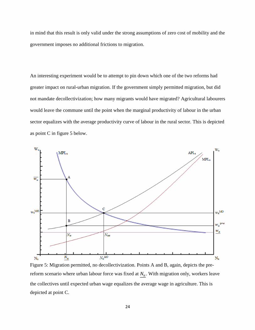
not mandate decollectivization; how many migrants would have migrated? Agricultural labourers

would leave the commune until the point when the marginal productivity of labour in the urban

sector equalizes with the average productivity curve of labour in the rural sector. This is depicted

as point C in figure 5 below.

Figure 5: Migration permitted, no decollectivization. Points A and B, again, depicts the pre-

reform scenario where urban labour force was fixed at 𝑁𝑢 . With migration only, workers leave

the collectives until expected urban wage equalizes the average wage in agriculture. This is

depicted at point C.

25

So far, we have made the strong assumptions of zero movement costs along with no government

imposed movement frictions.

4.3 Frictions to Migration: Costs and Obstacles

Rural to urban migration is not a free process; even without any government or externally

imposed obstacles, migrants will face movement costs such as transportation expenses, disutility

from leaving family home. Even upon reaching the urban sector, migrant workers face strong

discrimination in the urban sector. They do not have access to any of the institutional supports

such as child care, healthcare, unemployment benefits, nor are they able to collectively bargain

wages. These frictions which occur as a part of the movement without externally imposed

obstacles are considered to be “natural frictions” in this model. Intuitively, these natural frictions

will reduce the number of migrants.

Let 𝜃 denote this natural frictions parameter, expressed as a proportion of the expected urban

payout, 0 ≤ 𝜃 < 1.

We are also assuming that all workers in the rural sector face the same natural frictions. No

potential migrant have any advantage they could exploit when migrating to the urban sector.

The equilibrium migration condition between the urban and agricultural sector is now modified

to the following:

1 − 𝜃 𝛼𝐵𝐿𝑢(𝛼−1) = 𝛼𝐴𝐿𝑎

(𝛼−1) (13)

The left hand side is the modified urban expected payout and right hand side is the agricultural

wage. This equation implies that if 𝜃 is some positive constant then the payoffs from migration

26

decreases. With reduced payoffs from migration, then in equilibrium, the urban sector will be

smaller than the perfectly competitive case as less rural workers are willing to migrate.

Solving for (13) with the population condition (8) yields the labour force in the urban sector with

natural frictions:

𝐿𝑢𝑁𝐹 =

𝐵(1 − 𝜃)𝐴

11−𝛼

1 + 𝐵(1 − 𝜃)

𝐴

11−𝛼

𝑁

The labour force in agriculture with natural frictions is:

𝐿𝑎𝑁𝐹 =

1

1 + 𝐵(1 − 𝜃)

𝐴

11−𝛼

𝑁

The wage in the urban sector is:

𝑤𝑢𝑁𝐹 = 𝐵

𝐵(1 − 𝜃)𝐴

11−𝛼

1 + 𝐵(1 − 𝜃)

𝐴

11−𝛼

𝑁

−1+𝛼

𝛼

And wage in rural sector is:

𝑤𝑎𝑁𝐹 = 𝐴

1

1 + 𝐵(1 − 𝜃)

𝐴

11−𝛼

𝑁

−1+𝛼

𝛼

27

In competitive equilibrium with natural frictions, expected wages across both sectors equalizes at

a level below the case without natural frictions as there are obstacles in the urban sector which

imposes extra costs for workers who wishes to move into it.

𝑤𝑢𝑁𝐹 = 𝑤𝑎

𝑁𝐹 < 𝑤𝑢𝑐𝑜𝑚𝑝 = 𝑤𝑎

𝑐𝑜𝑚𝑝

This competitive equilibrium with natural friction is depicted in figure 6 below.

Figure 6: Competitive case with migration frictions. Ec depicts the competitive equilibrium

without migration frictions. MPLuNF

denotes the urban labour demand curve with the natural

friction parameter. The competitive equilibrium with migration frictions is the point ENF

when

the marginal productivity of urban labour with natural friction equalizes with the marginal

productivity of labour in agriculture.

28

4.4 Urban Wage Rigidities

The reason for the government to impose additional rigidities is to maintain the wage

level of urban sector at a level same as before migrations were permitted. People in the urban

sector were considered of higher class and held political sway over the government. The Chinese

central government’s first priority above all else is to stay in power; therefore, they had to keep

the urban population relatively happy. The government must prevent migrants from flooding the

urban sector labour supply, which would depress the urban wage. A sudden influx of people into

the urban cities would also stress its infrastructure which could cause the local residents

additional problems such as congestion and shortages of clean water and electricity. The Chinese

central government would have to control migration so the wage in the urban sector maintains at

the level without migration in order to keep the urban residents happy.

The central government could impose frictions in addition to the natural frictions to

maintain urban wages. These frictions would be imposing costs in some way to the migrants

either directly or directly. A direct example would be, since not all migrants migrated legally

through the Hukou process, there would be a probability that a migrant could be deported, which

would reduce the expected payouts to migration. This policy would also reduce expected

migration payout indirectly as firms who hire migrants know that there is a probability that these

workers will be detected as illegal and kicked out. This creates an extra cost for the firm as the

turnover rate will increase. Firms will pass this cost on to the migrant workers by paying them a

lower wage. Let 𝜙 denote any additional government imposed frictions to migration, 0 ≤ 𝜙 < 1.

The equilibrium migration condition between the urban and rural sector is now:

1 − (𝜃 + 𝜙) 𝛼𝐵𝐿𝑢𝛼−1 = 𝛼𝐴𝐿𝑎

(𝛼−1) (14)

29

Recall that 𝜃 denote the natural frictions to migration, equation (14) combines both the natural

frictions to migration in addition to the government imposed frictions. 𝜃 + 𝜙 < 1 is imposed

to prevent the frictions from being greater than the urban expected payout.

The government takes natural frictions as is, so 𝜃 is exogenous; 𝜙 is the government choice

variable. If the government wishes to pick 𝜙 at a level which keeps urban wage at the same level

as before the 1978 economic reforms, they must forcibly impose urban labour force to same as

before, at 𝐿𝑢 = 𝑁𝑢 . Solving for the government imposed friction yields the following:

𝜙 = 1 − 𝜃 −𝐴

𝐵 (

𝐿𝑢

𝑁 − 𝐿𝑢)(1−𝛼)

With this new government imposed friction parameter, the expected returns from migration to

the urban sector is reduced further. The total friction faced by the migrant is as following:

𝜃 + 𝜙 = 1 −𝐴

𝐵 (

𝐿𝑢

𝑁 − 𝐿𝑢)1−𝛼

Figure 7 below illustrates the scenario where government chooses the 𝜙 parameter to a level

which lowers the expected payout from migration so far that none would migrate.

30

Figure 7: Government chooses a 𝜙 which lowers expected payout to migration to a level where a

rural migrant will not be made better off by migrating.

All of this seems paradoxical, what is the point of permitting migration if the government

has to hold urban labour force fixed to exactly the same level as before migration was permitted

in order to maintain the urban wage? What we are missing is the fact that after the 1978

economic reforms, both the rural the urban sector experienced rapid technological growth. The

urban sector could absorb more workers once its industries became more efficient and labour

intensive.

31

4.5 Urban Technological Growth

Since the 1978 economic reforms, agricultural productivity increased significantly due to

decollectivization of agriculture and government abandonment of agricultural price control. In

the urban sector, with the shift from capital intensive heavy industries to more labour intensive

consumer goods industries, demand for labour increased drastically (Wu & Yao 2003). Labour

augmenting technologies drove up productivity multiple folds. Technological growth in the

urban sector greatly outpaced developments in the agricultural sector. Let g denote the

technological growth parameter. For simplicity the following analysis ignores growth in the

agricultural sector. Then the equilibrium can be rewritten as:

1 + 𝑔 𝛼𝐵𝑁𝑢(𝛼−1) = 𝛼𝐴𝑁𝑎

(𝛼−1)

We have previously assumed downward rigidity on the urban wage. Now let us say that urban

residents will be happy as long as their wages do not decrease, so that even with technological

improvement which enhances labour productivity, urban sector wage remains fixed. Urban wage

is then fixed at the same level as before the 1978 reforms, 𝑤𝑢 .

Recall from the pre-reform case:

𝑤𝑢 = 𝐵𝑁𝑢−1+𝛼𝛼

We can now set the new labour demand curve equal to the fixed pre-reform wage level:

1 + 𝑔 𝛼𝐵𝑁𝑢(𝛼−1) = 𝐵𝑁𝑢

−1+𝛼𝛼

Solving for the new labour force in urban sector with technological growth and fixed urban

wages yields:

32

𝑁𝑢𝑇𝐹 = 𝑁𝑢(1 + 𝑔)(

11−𝛼

)

where 𝑁𝑢𝑇𝐹 denote urban population with technological growth.

As the marginal productivity functions are strictly convex, increases in technology transfers to

more workers employed in the urban sector, the magnitude of this conversion depends on the

production parameter α.

The increase of urban sector workers is:

𝛥𝑁𝑢 = 1 + 𝑔 1

1−𝛼 𝑁𝑢 − 𝑁𝑢

The enlargement of the urban sector will have implications on rural labour force and wages.

Substituting the new urban labour force 𝑁𝑢𝑇𝐹 into the agricultural labour force condition (10)

yields the agricultural labour force with technological growth:

𝑁𝑎𝑇𝐹 = 𝑁 − 𝑁𝑢(1 + 𝑔)(

11−𝛼

)

As 𝑁𝑢(1 + 𝑔)(1

1−𝛼) > 𝑁𝑢 , the new agricultural sector is now smaller.

Agricultural wage also changes with this new lower level of agricultural labour force.

Substituting the new agricultural labour force 𝑁𝑎𝑇𝐹 into agricultural MPL equation (2) yields:

𝑤𝑎𝑇𝐹 = 𝛼𝐴(𝑁 − 𝑁𝑢 1 + 𝑔

11−𝛼

)𝛼−1

Where 𝑤𝑎𝑇𝐹 denote the wage in agriculture, which also increases as the agricultural labour force

decreases.

33

Figure 8 below depicts this outcome,

Figure 8: Increased urban labour demand with technological growth. MPLu is the original urban

labour demand curve and MPLuTF

is the urban demand curve with technological growth. 𝑤𝑢 is

fixed at the pre-reform level. Points A and B denote the urban and rural wages associated with

the no technological growth labour demand curve. This result is same as the case before the 1978

economic reforms waNT

denote the agricultural wage with no technological growth. Points C and

E are urban and agricultural wage results for the new level of urban labour force 𝑁𝑢𝑇𝐹 , which is

associated with the new labour demand curve, MPLuTF

. 𝑤𝑎𝑇𝐹 is the wage in agriculture with

technological growth. The distance between C and D depicts the technological improvement.

The result depicted here is very important as it illustrates that urban development, which

increases urban labour demand, will not only improve the situation in the urban sector, but will

34

also increase the wage in the rural sector. This implies that urban-focused development will not

exacerbate the problems of rural poverty; on the contrary, it will alleviate this persistent problem.

Finally, if we assume that even at the higher level of urban labour force, 𝑁𝑢𝑇𝐹 , it is still below

the competitive equilibrium, then it is of interest to determine what level of government friction

required to keep urban labour force at the new level of 𝑁𝑢𝑇𝐹 . The government friction parameter,

ϕ is solved as the following:

𝜙 = 1 − 𝜃 −𝐴

𝐵 (

𝑁𝑢𝑇𝐹

𝑁 − 𝑁𝑢𝑇𝐹)(1−𝛼)

The government friction choice parameter here is smaller than the case without technological

growth since 𝑁𝑢𝑇𝐹 > 𝑁𝑢 . This is the desired result as it shows that since the urban sector is able

to employee more workers, then in order for the government to maintain the urban wage, smaller

friction is required compared to the case where urban sector could only employee its own

population.

35

5. Conclusion

The greatest rural to urban migration in human history is happening right now in the

world’s fastest growing economy, China. The Lewis and Harris-Todaro models provide an

excellent foundation to modeling the migration history of China. This paper builds a simple

theoretical model while drawing upon assumptions and findings of the Lewis and H-T models.

The two-sector model built in this paper was able to depict the interactions between the rural and

urban sectors in China in the years of Mao Zedong (1949-1978), the catastrophic years of “The

Great Leap Forward” (1958-1961), and the economic reforms of Deng Xiaoping (1978). The rich

history of China makes it difficult to model all its unique aspects. This unique history makes

drawing policy conclusions an even greater challenge. The conclusion of this paper is similar to

the Lewis model’s conclusion of technological growth being the most consistent driving force of

growth. The Lewis model favours agricultural development as the best prescription to

developing nations. The model constructed in this paper illustrates that urban development,

which is a more politically feasible policy, will achieve the goal of alleviating rural poverty and

mitigate rural-urban wage differential. This conclusion is drawn under the assumption that there

is sufficient high agricultural output that there are no food shortages. This assumption is true in

China; however, this is not the case in many other developing nations. Therefore it is important

to analyze agricultural surplus before applying this policy to other developing countries with

excess rural workers.

36

References

Harris, J., and Todaro, M. (1970). “Migration, Unemployment, and Development: A Two-Sector

Analysis,” American Economic Review 40, 126-142.

Knight, J. (2007). China, South Africa and the Lewis Model. The Centre for the Study of African

Economies Working Paper Series, 271. Retrieved from

http://www.bepress.com/csae/paper271

Lewis, W. A. (1954). “Economic Development with Unlimited Supplies of Labor,” The

Manchester School of Economics and Social Studies 22, 139-191.

Malthus, T. R. (1826), “An Essay on the Principle of Population: A View of its Past and Present

Effects on Human Happiness; with an Inquiry into Our Prospects Respecting the Future

Removal or Mitigation of the Evils which It Occasions” (Sixth ed.), London: John Murray.

Prasad, S. (2009). "Is the Chinese Growth Miracle Built to Last," Chinese Economic Review,

20(1), 102-123.

Ranis, G (2004), “Arthur Lewis’s Contribution to Development Thinking and Policy,” The

Manchester School, Vol. 72, No. 6 (December), pp. 712-723

Rawski, T. (1999). China’s Economy After Fifty Years: Retrospect and Prospect. Retrieved from

http://www.pitt.edu/~tgrawski/paper99/rawski-intlj.htm

Wei, L. and D. T. Yang (2005). "The Great Leap Forward: Anatomy of a central planning

disaster," Journal of Political Economy 113 (4), 840–877.

Wu, Z., & Yao, S. (2003). "Intermigration and intramigration in China: A theoretical and

empirical analysis," China Economic Review, 14, 371-385.

Xu, Y (1994). “Trade Liberalization in China: A CGE Model with Lewis Rural Surplus Labor,”

China Economic Review, Vol. 5, No. 2, pp. 205-219