RTE DSE – Protection Demonstration
166
RTE DSE – Protection Demonstration Final Project Report T-59G Power Systems Engineering Research Center Empowering Minds to Engineer the Future Electric Energy System
Transcript of RTE DSE – Protection Demonstration

RTE DSE – Protection Demonstration
Final Project Report
T-59G
Power Systems Engineering Research Center Empowering Minds to Engineer
the Future Electric Energy System

RTE DSE – Protection Demonstration
Final Project Report
Project Team Sakis Meliopoulos, Project Leader
George Cokkinides Georgia Institute of Technology
Graduate Students Jiahao Xie Yuan Kong
Georgia Institute of Technology
PSERC Publication 18-09
September 2018

For information about this project, contact: Sakis A.P. Meliopoulos Georgia Institute of Technology School of Electrical and Computer Engineering Dept Mail Code: 0250 777 Atlantic Dr NW Atlanta, GA 30332 Phone: 404-894-2926 E-mail: [email protected] Power Systems Engineering Research Center The Power Systems Engineering Research Center (PSERC) is a multi-university Center conducting research on challenges facing the electric power industry and educating the next generation of power engineers. More information about PSERC can be found at the Center’s website: http://www.pserc.org. For additional information, contact: Power Systems Engineering Research Center Arizona State University 527 Engineering Research Center Tempe, Arizona 85287-5706 Phone: 480-965-1643 Fax: 480-727-2052 Notice Concerning Copyright Material PSERC members are given permission to copy without fee all or part of this publication for internal use if appropriate attribution is given to this document as the source material. This report is available for downloading from the PSERC website.
2018 Georgia Institute of Technology. All rights reserved.

i
Acknowledgements
This targeted PSERC research project was funded by RTE. We express our appreciation to RTE, and especially to Patrick Pancitici, Thibault Prevost, Aurelien Watare, and Christian Guibout for their support and guidance. We also express our appreciation for the support provided by RTE members and PSERC members.

ii
Executive Summary
This report describes the application of setting-less relay on the RTE digital substation. We describe the model developed to simulate various events, and then play back these events into the setting-less relays to assess their performance. Four protection zones have been identified within the RTE digital substation. Use cases for each one of these protection zones have been developed with multiple events. The protection of each one of these protection zones has been studied under multiple events. Sample use cases of this testing is included in this report. A new methodology for correcting measurement errors from the instrumentation has been also developed and tested. The basic idea of the setting-less protection relay has been inspired from the differential protection function which has a very important characteristic: it does not require coordination with any other protection functions. The differential protection monitors the validity of Kirchhoff’s current law (KCL) within a protection zone. The setting-less protection can be considered as an extension and generalization of differential protection, because it can be viewed as monitoring the validity of all physical laws within the protection zone, i.e. KCL, KVL, thermodynamics, mechanical motion, etc. depending on the type of protection zone. The setting-less relay does not require coordination with any other protection function, a very big advantage. The setting-less relay replaces all the protection functions that are typically apply to a protection use using legacy protection systems. Four protection zones have been identified within the RTE digital substation. The protection of these four zones has been studied extensively with numerical experiments as well as in the laboratory with hardware in the loop. In these studies we used a number of simulated test events. For the generation of the test events, a model of the RTE digital substation and the interconnected 220 kV and 90 kV system has been modeled with equivalent sources at the ends of the 220 kV and 90 kV transmission circuits. The model has been developed in WinIGS-T format (time domain). The report provides an overview of the model and the parameters of the major devices and the definition of the protection zones. The majority of the model parameters were provided by RTE. For missing parameter values, typical values were used. The model has been used to develop a large number of events for the purpose of testing the setting-less relay application on various protection zones of the RTE digital substation. A small number of these events are documented in a number of use cases which are included in this report. For secure and reliable protection of power components such as a generator, line, transformer, etc. a new approach has emerged based on component health dynamic monitoring. The proposed method uses dynamic state estimation, based on the dynamic model of the component, which accurately reflects the nonlinear characteristics of the component as well as the loading and thermal state of the component. The performance of any protection system is always dependent upon the quality and validity of the measurements, i.e. the input data into the relay. This has been recognized for any protective system and it is valid for the setting-less relays. The introduction of merging units offers a powerful way of correcting the measured sampled values in real time. Specifically, the model of the instrumentation channel can be used in a dynamic state estimation procedure to provide the estimated values of the primary quantities from the secondary quantities. This task can be

iii
performed on each one of the instrumentation channels independently from any other channel, i.e. it is a distributed computation process and it does not affect the operation of the relay other than a small latency that is only a fraction of the sampling period. The process provides the best estimate of the primary sampled values. The report describes the implementation of the method and demonstrates the method on an example test system. It is shown that the method performs remarkably well even in cases of severe saturation of instrument transformers. Project Publications: [1] A. P. Sakis Meliopoulos, George Cokkinides, Jiahao Xie, and Yuan Kong,
"Instrumentation Error Correction within Merging Units", Proceedings of the 2018 Georgia Tech Fault and Disturbance Analysis Conference, Atlanta, Georgia, April 30-May 1, 2018.
[2] A. P. Sakis Meliopoulos, G. J. Cokkinides, Hussain Albinali, Paul Myrda and Evangelos Farantatos, “Integrated Centralized Substation Protection”, Proceedings of the of the 51th Annual Hawaii International Conference on System Sciences, Hawaii, HI, January 3-6, 2018.
Student Theses: [1] Yuan Kong. Instrumentation Error Correction and its Effects on Transmission, PhD,
Georgia Institute of Technology, 2019 (expected). [2] Jiahao Xie. Centralized Substation Protection, PhD, Georgia Institute of Technology,
Expected Graduation: 2019 (expected).

i
Table of Contents
1. Introduction ................................................................................................................................1
1.1 Background ........................................................................................................................1
1.2 Overview of the Problem ...................................................................................................1
1.3 Report Organization ..........................................................................................................1
2. The Setting-less Protective Relay ...............................................................................................3
2.1 Setting-less Relay Testing with Hardware in the Loop .....................................................4
2.2 Data Correction within Merging Units ..............................................................................8
3. Sample Value Data Correction ...................................................................................................9
3.1 Method Description ...........................................................................................................9
3.2 Example Results...............................................................................................................13
4. Application to the RTE System ................................................................................................17
5. Example Test Results, RTE Protection Zone 1 ........................................................................22
5.1. Creating Protection Zone Models for EBP Relays ...........................................................23
5.1.1 Creating the Network Time Domain Model ..........................................................23
5.1.2 Creating Measurement Models for Merging Units ...............................................27
5.1.3 Exporting Measurement and Protection Zone Models ..........................................38
5.2 Creating Events and Storing in COMTRADE ..................................................................40
5.2.1 Event A: UseCase_01.A ........................................................................................40
5.2.2 Event B: UseCase_01.B ........................................................................................45
5.3 EBP Results .....................................................................................................................49
5.3.1 Event A: UseCase_01.A ........................................................................................49
5.3.2 Event B: UseCase_01.B ........................................................................................54
6. Example Test Results: RTE Protection Zone 04 .....................................................................60
6.1 Creating Protection Zone Models for EBP Relays ...........................................................61
6.1.1 Creating the Network Time Domain Model ...........................................................61
6.1.2 Creating Measurement Models for Merging Units ...............................................65
6.1.3 Exporting Measurement and Protection Zone Models ..........................................76
6.2 Creating Events and Storing in COMTRADE ..................................................................78
6.2.1 Event A: UseCase_01.A ........................................................................................78
6.2.2 Event B: UseCase_01.B ........................................................................................81
6.3 EBP Results .......................................................................................................................83

ii
6.3.1 Event a: UseCase_01.A .........................................................................................83
6.3.2 Event b: UseCase_01.B .........................................................................................89
7. Summary, Conclusions and Future Work ..................................................................................94
Appendix A: RTE Model: Device List and Parameters .................................................................95
Appendix B: BLOCAUX Substation 225 kV Section ...................................................................99
Appendix C: BLOCAUX Substation 90 kV Section ...................................................................107
Appendix D: Cables Between 225 kV and 90 kV Section ..........................................................108
Appendix E: 225 kV External System .........................................................................................111
Appendix F: 90 kV External System ...........................................................................................116
Appendix G: Definition of Protection Zones Under Consideration ............................................124
Protection Zone 1 ...................................................................................................................125
Protection Zone 2 ...................................................................................................................134
Protection Zone 3 ...................................................................................................................141
Protection Zone 4 ...................................................................................................................148
References ....................................................................................................................................152

iii
List of Figures
Figure 2-1: Conceptual Description of the Estimation Based Protection ....................................... 3
Figure 2-2: Block Diagram of Estimation Based Relay ................................................................. 5
Figure 2-3 Photograph of the PSCAL (Power System Control and Automation Laboratory) ....... 6
Figure 2-4: Example Visualizations of a Setting-less Relay Applied to a Transformer ................. 7
Figure 2-5: Error Correction within Merging Units ....................................................................... 8
Figure 3-1: Instrumentation Channel Subsystem – Voltage and Current Instrumentation Channel ........................................................................................................................................... 9
Figure 3-2: Typical Current Instrumentation Channel Configuration ......................................... 11
Figure 3-3: Equivalent Circuit of CT’s Primary Current Estimation .......................................... 11
Figure 3-4: Example System for Current Instrumentation Channel Error Correction................. 13
Figure 3-5: CT Secondary Current through the Burden Resistor ................................................. 14
Figure 3-6: Comparison between the CT Primary Current before and after Correction .............. 15
Figure 3-7: CT Secondary Current through the Burden Resistor ................................................. 15
Figure 3-8: Comparison between the CT Primary Current before and after Correction .............. 16
Figure 4-1: The RTE Subsystem Single Line Diagram ................................................................ 17
Figure 4-2: Single Line Diagram of 225 kV Section .................................................................... 18
Figure 4-3: Single Line Diagram of 90 kV Section ...................................................................... 18
Figure 4-4: RTE – BLOCAUX Substation – Protection Zone 1 .................................................. 19
Figure 4-5: RTE – BLOCAUX Substation – Protection Zone 2 .................................................. 20
Figure 4-6: RTE – BLOCAUX Substation – Protection Zone 3 .................................................. 20
Figure 4-7: RTE – BLOCAUX Substation – Protection Zone 4 .................................................. 21
Figure 5-1: Single Line Diagram of Protection Zone 1 ................................................................ 24
Figure 5-2: Parameters of the Three-Phase Three-Winding Transformer .................................... 25
Figure 5-3: Parameters of the Three-Phase Cable ........................................................................ 26
Figure 5-4: Merging Unit Main Parameter Dialog ....................................................................... 27
Figure 5-5: Merging Unit Instrumentation Channel List Dialog .................................................. 28
Figure 5-6: Example of a Voltage Instrumentation Channel Dialog ............................................ 28
Figure 5-7: Example of a Current Instrumentation Channel Dialog ............................................. 29
Figure 5-8: Instrument Transformer Library Dialog .................................................................... 32
Figure 5-9: Example Input Specifications of a GE MU320 Merging Unit ................................... 33
Figure 5-10: Measurement List Dialog ......................................................................................... 34

iv
Figure 5-11: Voltage Measurement Parameters Dialog ................................................................ 35
Figure 5-12: Current Measurement Parameters Dialog ................................................................ 35
Figure 5-13: Selecting Zone Power Devices and Merging Units ................................................. 38
Figure 5-14: EBP Export Dialog................................................................................................... 39
Figure 5-15: Message Window Indicating EBP File Creation Progress & File Paths .................. 39
Figure 5-16: Network Model with Fault between Phase A and Neutral at Bus TRNS1~90 ........ 40
Figure 5-17: Time Domain Simulation Parameters Dialog .......................................................... 41
Figure 5-18: Voltage and Current Measurements Obtained from Merging Unit 1 in Event A .... 42
Figure 5-19: Voltage and Current Measurements Obtained from Merging Unit 2 in Event A .... 43
Figure 5-20: Voltage and Current Measurements Obtained from Merging Unit 3 in Event A .... 44
Figure 5-21: Network Model with Fault between Phase A and Neutral at Bus A225D2 ............. 45
Figure 5-22: Voltage and Current Measurements Obtained from Merging Unit 1 in Event B .... 46
Figure 5-23: Voltage and Current Measurements Obtained from Merging Unit 2 in Event B .... 47
Figure 5-24: Voltage and Current Measurements Obtained from Merging Unit 3 in Event B .... 48
Figure 5-25: Opening the EBP Main Setup Form in the WinXFM Program ............................... 49
Figure 5-26: Importing Zone 1 Device and Measurement Definition Files ................................. 50
Figure 5-27: Opening the COMTRADE Setup Dialog................................................................. 51
Figure 5-28: Selecting the COMTRADE Data Files for Playback ............................................... 51
Figure 5-29: Plots of Some Actual/Estimated Measurements, Residuals, Confidence Level, and Trip Decision in Event A ....................................................................................................... 52
Figure 5-30: A List of Available Channels for Plotting ............................................................... 53
Figure 5-31: Importing Zone 1 Device and Measurement Definition Files ................................. 55
Figure 5-32: Opening the COMTRADE Setup Dialog................................................................. 56
Figure 5-33: Selecting the COMTRADE data files for Playback ................................................. 57
Figure 5-34: Plots of Some Actual/Estimated Measurements, Residuals, Confidence Level, and Trip Decision in Event B ........................................................................................................ 58
Figure 5-35: A List of Available Channels for Plotting ............................................................... 59
Figure 6-1: RTE System Network Model ..................................................................................... 62
Figure 6-2: RTE Substation Single Line Diagram (top) and Protection Zone 04 (bottom) ......... 63
Figure 6-3: Protection Zone 4 Parameters .................................................................................... 64
Figure 6-4: Merging Unit Main Parameter Dialog ....................................................................... 65
Figure 6-5: Merging Unit Instrumentation Channel List Dialog .................................................. 66
Figure 6-6: Example of a Voltage Instrumentation Channel Dialog ............................................ 66

v
Figure 6-7: Example of a Current Instrumentation Channel Dialog ............................................. 67
Figure 6-8: Instrument Transformer Library Dialog .................................................................... 70
Figure 6-9: Example Input Specifications of A GE MU320 Merging Unit ................................. 71
Figure 6-10: Measurement List Dialog ......................................................................................... 72
Figure 6-11: Voltage Measurement Parameters Dialog ................................................................ 73
Figure 6-12: Current Measurement Parameters Dialog ................................................................ 73
Figure 6-13: Selecting Zone Power Devices and Merging Units ................................................. 76
Figure 6-14: EBP Export Dialog................................................................................................... 77
Figure 6-15: Message Window Indicating EBP File Creation Progress & File Paths .................. 77
Figure 6-16: Network Model with Fault between Phase A and Neutral of REACTOR Bus ....... 78
Figure 6-17: Time Domain Simulation Parameters Dialog. ......................................................... 79
Figure 6-18: Time Domain Simulation Output Plot for Event A ................................................. 80
Figure 6-19: Network Model with Fault between Phase A and Neutral of Bus A225D2. ........... 81
Figure 6-20: Time Domain Simulation Output Plot for Event B.................................................. 82
Figure 6-21: Opening the EBP Main Setup Form in the WinXFM Program ............................... 83
Figure 6-22: Importing Zone 4 Device and Measurement Definition Files ................................. 84
Figure 6-23: Opening the COMTRADE Setup Dialog................................................................. 85
Figure 6-24: Selecting the COMTRADE data files for Playback ................................................. 85
Figure 6-25: Starting the EBP Relay Using Playback Data (COMTRADE)................................ 86
Figure 6-26: Plots of Measurement and Estimated Values, Confidence Level and Trip Decision during Event A ............................................................................................................... 87
Figure 6-27: Available Data for Plotting on the Main WinXFM Window................................... 88
Figure 6-28: Importing Zone 4 Device and Measurement Definition Files ................................. 89
Figure 6-29: Opening the COMTRADE Setup Dialog................................................................. 90
Figure 6-30: Selecting the COMTRADE Data Files for Playback ............................................... 91
Figure 6-31: Starting the EBP Relay Using Playback Data (COMTRADE)................................ 92
Figure 6-32: Plots of Measurement and Estimated Values, Confidence Level and Trip Decision during Event B ............................................................................................................... 93
Figure A-1: Single Line Diagram of the RTE System including the BLOCAUX Substation and Its External Links ................................................................................................................... 98
Figure B-1: Single Line Diagram of 225 kV Section ................................................................... 99
Figure B-2: 245 kV Shunt Reactor Parameters........................................................................... 100
Figure B-3: 225/93/10.5 kV Transformer 641 Parameters ......................................................... 101

vi
Figure B-4: 225/93/9.9 kV Transformer 642 Parameters ........................................................... 102
Figure B-5: 225/93/10.0 kV Transformer 643 Parameters ......................................................... 103
Figure B-6: 2 Winding Transformer 1 Parameters ..................................................................... 104
Figure B-7: 2 Winding Transformer 2 Parameters ..................................................................... 105
Figure B-8: 2 Winding Transformer 3 Parameters ..................................................................... 106
Figure C-1: Single Line Diagram of 90 kV Section ................................................................... 107
Figure D-1: 90 kV cable 1 Parameters, Inside Substation .......................................................... 108
Figure D-2: 90 kV cable 2 Parameters, Inside Substation .......................................................... 109
Figure D-3: 90 kV cable 3 Parameters, Inside Substation .......................................................... 110
Figure E-1: Single Line Diagram of the External 225 kV System ............................................. 111
Figure E-2: 225 kV Source Limeux Parameters ......................................................................... 112
Figure E-3: 225 kV Source Argeouves Parameters .................................................................... 113
Figure E-4: 225 kV Trasmission Line From S-Limeux to Limeux Parameters ......................... 114
Figure E-5: 225 kV Trasmission Line From Argeouves to S-Argevs Parameters ..................... 115
Figure F-1: Single Line Diagram of the External 90 kV System ............................................... 116
Figure F-2: 90 kV Transmission Line From Fouilloy1 to L-Fouillo Parameters ....................... 117
Figure F-3: 90 kV Transmission Line From L-Croixra to Croixraul Parameters ....................... 118
Figure F-4: 90 kV Transmission Line From L-Bourbel to Bourbel Parameters......................... 119
Figure F-5: 90 kV Transmission Line From L-Aumale1 to Aumale1 Parameters ..................... 120
Figure F-6: 90 kV Transmission Line From Alleux~F2 to L-Allx-F2 Parameters .................... 121
Figure F-7: 90 kV Transmission Line From Alleux1 to L-Alleux1 Parameters......................... 122
Figure F-8: 90 kV Transmission Line From L-NFCHAUM to NFCH~AUM2 Parameters ...... 123
Figure G-1: Protection Zone 1 .................................................................................................... 125
Figure G-2: 225 kV / 93 kV / 10.5 kV Transformer 641 Parameters ......................................... 126
Figure G-3: 90 kV Cable 1 Parameters ....................................................................................... 127
Figure G-4: Merging Unit 1 (Captures the Measurements of 225 kV/93 kV /10.5 kV Transformer 641) ........................................................................................................................ 128
Figure G-5: Instrumentation Channels of Merging Unit 1 ......................................................... 129
Figure G-6: Measurement Channels of Merging Unit 1 ............................................................. 129
Figure G-7: Merging Unit 2 (Captures the Measurements of 90 kV Cable 1) .......................... 130
Figure G-8: Instrumentation Channels of Merging Unit 2 ......................................................... 131
Figure G-9: Measurement Channels of Merging Unit 2 ............................................................. 131
Figure G-10: Merging Unit 8 (captures the voltage measurements of bus B1B2~225 kV) ....... 132

vii
Figure G-11: Instrumentation Channels of Merging Unit 8 ....................................................... 133
Figure G-12: Measurement Channels of Merging Unit 8 ........................................................... 133
Figure G-13: Protection Zone 2 .................................................................................................. 134
Figure G-14: 225 kV / 93 kV Transformer 642 Parameters ....................................................... 135
Figure G-15: 90 kV Cable 2 Parameters ..................................................................................... 136
Figure G-16: Merging Unit 3 (Captures the Measurements of 225 kV/93 kV Transformer 642) ............................................................................................................................................. 137
Figure G-17: Instrumentation Channels of Merging Unit 3 ....................................................... 138
Figure G-18: Measurement Channels of Merging Unit 3 ........................................................... 138
Figure G-19: Merging Unit 4 (Captures the Measurements of 90 kV Cable 2) ......................... 139
Figure G-20: Instrumentation Channels of Merging Unit 4 ....................................................... 140
Figure G-21: Measurement Channels of Merging Unit 4 ........................................................... 140
Figure G-22: Protection Zone 3 .................................................................................................. 141
Figure G-23: 225 kV / 93 kV Transformer 643 Parameters ....................................................... 142
Figure G-24: 90 kV Cable 3 Parameters ..................................................................................... 143
Figure G-25: Merging Unit 5 (Capture the Measurements of 225 kV/93 kV Transformer 643) ............................................................................................................................................. 144
Figure G-26: Instrumentation Channels of Merging Unit 5 ....................................................... 145
Figure G-27: Measurement Channels of Merging Unit 5 ........................................................... 145
Figure G-28: Merging Unit 6 (Captures the Measurements of 90 kV Cable 3) ......................... 146
Figure G-29: Instrumentation Channels of Merging Unit 6 ....................................................... 147
Figure G-30: Measurement Channels of Merging Unit 6 ........................................................... 147
Figure G-31: Protection Zone 4 .................................................................................................. 148
Figure G-32: 245 kV Shunt Reactor Parameters ........................................................................ 149
Figure G-33: Merging Unit 7 (Captures the Measurements of 245 kV Shunt Reactor) ............. 150
Figure G-34: Instrumentation Channels of Merging Unit 7 ....................................................... 151
Figure G-35: Measurement Channels of Merging Unit 7 ........................................................... 151

viii
List of Tables
Table 5-1: Instrumentation Channel Parameters – User Entry Fields .......................................... 30
Table 5-2: Measurement Parameters – User Entry Fields ............................................................ 36
Table 5-3: Instrumentation Channels of Merging Units in Protection Zone 1 ............................. 37
Table 6-1: Instrumentation Channel Parameters – User Entry Fields .......................................... 68
Table 6-2: Measurement Parameters – User Entry Fields ............................................................ 74
Table A-1: Tabulation of Major Devices Included in the Model ................................................. 95

1
1. Introduction
1.1 Background
Georgia Tech and EPRI, over the last few years, they have been developing the Dynamic State Estimation based protection method (a.k.a. setting-less protection). This technology has been demonstrated in the laboratory and also a demonstration project with NYPA under NYSERDA sponsorship is in progress. The objective of the proposed project is to demonstrate the technology on the digital substation that RTE is developing. A DSE based relay has been developed for the protection of selected protection zones of the RTE’s digital substation and factory tested at the Georgia Tech laboratory. The plan is to install this relay to an RTE substation. As of the end of this project, this installation has not been completed due to schedules beyond the control of the investigators. The plan is to install the relay in the field when the conditions will permit in the future. This report describes the application of setting-less relay on the RTE digital substation. The report describes the model developed to simulate various events, and then play back these events into the setting-less relays to assess their performance. Four protection zones have been identified within the RTE digital substation. Use cases for each one of these protection zones have been developed with multiple events. The protection of each one of these protection zones has been studied under multiple events. Sample use cases of this testing are included in this report.
1.2 Overview of the Problem
For the generation of the test events, a model of the RTE digital substation and the interconnected 220 kV and 90 kV system has been modeled with equivalent sources at the ends of the 220 kV and 90 kV transmission circuits. The model has been developed in WinIGS-T format (time domain). The report provides an overview of the model and the parameters of the major devices and the definition of the protection zones. The majority of the model parameters were provided by RTE. For missing parameter values, typical values were used. The model has been used to develop a large number of events for the purpose of testing the setting-less relay application on various protection zones of the RTE digital substation. A small number of these events are documented in a number of use cases which are included in this report.
1.3 Report Organization
The report is organized as follows: Section 2 provides a brief description of setting-less protection relay. Section 3 introduces the sample data correction method for the instrumentation channel. Section 4 together with Appendices A, B, C, D, E and F provides the parameters of the major devices included in the model. The EBP setting-up is also included in Section 4.

2
Section 5 and section 6 present a number of events for protection zones. The events include various fault and non-fault conditions and they are used for laboratory evaluation of the setting-less relays. Appendix G provides detailed description of protection zones of the BLOCAUX substation to be considered for implementation of the setting-less relay. It does not include all the protection zones of the substation.
3
2. The Setting-less Protective Relay
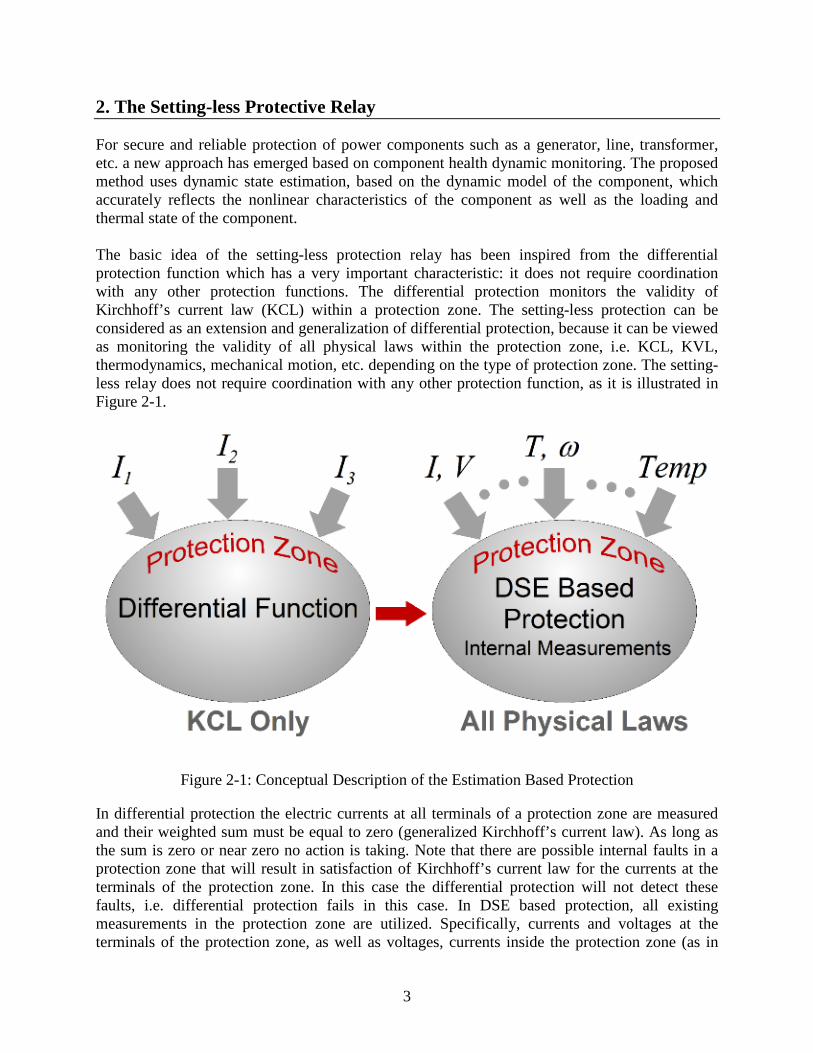
For secure and reliable protection of power components such as a generator, line, transformer, etc. a new approach has emerged based on component health dynamic monitoring. The proposed method uses dynamic state estimation, based on the dynamic model of the component, which accurately reflects the nonlinear characteristics of the component as well as the loading and thermal state of the component. The basic idea of the setting-less protection relay has been inspired from the differential protection function which has a very important characteristic: it does not require coordination with any other protection functions. The differential protection monitors the validity of Kirchhoff’s current law (KCL) within a protection zone. The setting-less protection can be considered as an extension and generalization of differential protection, because it can be viewed as monitoring the validity of all physical laws within the protection zone, i.e. KCL, KVL, thermodynamics, mechanical motion, etc. depending on the type of protection zone. The setting-less relay does not require coordination with any other protection function, as it is illustrated in Figure 2-1.
Figure 2-1: Conceptual Description of the Estimation Based Protection In differential protection the electric currents at all terminals of a protection zone are measured and their weighted sum must be equal to zero (generalized Kirchhoff’s current law). As long as the sum is zero or near zero no action is taking. Note that there are possible internal faults in a protection zone that will result in satisfaction of Kirchhoff’s current law for the currents at the terminals of the protection zone. In this case the differential protection will not detect these faults, i.e. differential protection fails in this case. In DSE based protection, all existing measurements in the protection zone are utilized. Specifically, currents and voltages at the terminals of the protection zone, as well as voltages, currents inside the protection zone (as in

4
capacitor protection) or speed, temperature and torque in case of rotating machinery or any other internal measurements. Then, the dynamic model of the device (consisting of physical laws such as KCL, KVL, motion laws, thermodynamic laws, etc.) is used to provide the inter-relationships among all measured quantities. When there is no fault within the protection zone, the measurements should satisfy the dynamic model of the protection zone. A dynamic state estimation procedure provides a systematic and mathematically rigorous way to verify that the measurements satisfy the mathematical model. When an internal fault occurs, the measurements do not fit the mathematical model of the protection zone and a protection action is triggered. The resulting method is a Dynamic State Estimation Based Protective relay (EBP relay). When an internal fault occurs, even high impedance faults or faults along a coil, etc., the dynamic state estimation reliably detects the abnormality and a trip signal can be issued. Three distinct dynamic state estimation algorithms (Extended Kalman Filter, Constraint Optimization and Unconstraint Optimization) have been developed and tested. Each algorithm requires the mathematical model of the protection zone, including instrumentation and the measurements. This basic approach has been extensively tested in the laboratory for several protection zones and presented in technical papers. It was named setting-less protection because of the simplicity of use and its lack of coordination issues with other relays, in the same way as differential protection does not require coordination. In addition, setting-less relays have been extensively tested in the laboratory with hardware in the loop.
2.1 Setting-less Relay Testing with Hardware in the Loop
Prototype setting-less protective relays have been developed in the laboratory, connected to a system represented with a simulator, digital to analog conversion, amplifiers and data acquisition systems (merging units). This setup enables testing with hardware in the loop. The setup consists of (a) merging units to perform data acquisition, (b) a process bus, and (c) a personal computer attached to the process bus and performing the protection functions (the personal computer “runs” the setting-less protection). The setting-less protective relay block diagram, as implemented in the laboratory is illustrated in Figure 2-2.

5
Figure 2-2: Block Diagram of Estimation Based Relay The physical system under protection (not shown in the figure) is simulated in the laboratory via a computer controlled system of digital to analog converters, amplifiers (we use Omicron amplifiers) that amplify the signal to relay instrumentation levels and then the signals are injected into the merging units, shown in Figure 2-2. From that point on, the setup uses actual equipment. The merging units are GE Hardfiber, Siemens or Reason (we can include more manufacturers of merging units as they become available). Merging units are connected to a process bus. A personal computer is connected to the process bus and retrieves the streaming data as they are reported by the merging units. The personal computer performs the setting-less protection functions and optionally displays the results or selective visualizations. The physical construction of the laboratory is shown in the photograph below.
6
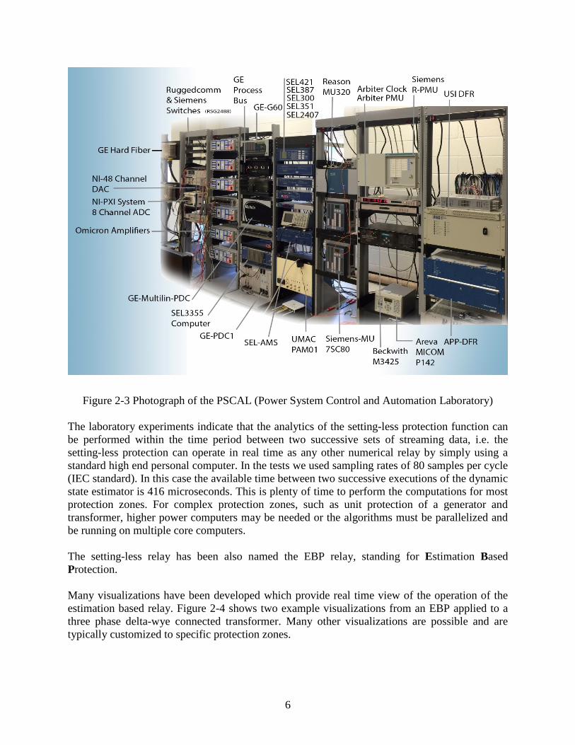
Figure 2-3 Photograph of the PSCAL (Power System Control and Automation Laboratory) The laboratory experiments indicate that the analytics of the setting-less protection function can be performed within the time period between two successive sets of streaming data, i.e. the setting-less protection can operate in real time as any other numerical relay by simply using a standard high end personal computer. In the tests we used sampling rates of 80 samples per cycle (IEC standard). In this case the available time between two successive executions of the dynamic state estimator is 416 microseconds. This is plenty of time to perform the computations for most protection zones. For complex protection zones, such as unit protection of a generator and transformer, higher power computers may be needed or the algorithms must be parallelized and be running on multiple core computers. The setting-less relay has been also named the EBP relay, standing for Estimation Based Protection. Many visualizations have been developed which provide real time view of the operation of the estimation based relay. Figure 2-4 shows two example visualizations from an EBP applied to a three phase delta-wye connected transformer. Many other visualizations are possible and are typically customized to specific protection zones.

7
Figure 2-4: Example Visualizations of a Setting-less Relay Applied to a Transformer The development of the EBP relay faced several challenges. A partial list of the challenges is given below. These challenges can be overcome with present technology. The project has demonstrated that these challenges are met.
1. Ability to perform the dynamic state estimation in real time 2. Initialization issues 3. Communications in case of a geographically extended component (i.e., lines) 4. New modeling approaches for components - connects well with the topic of modeling 5. Requirement for GPS synchronized measurements in case of multiple independent
data acquisition systems. The modeling issue is fundamental in this approach. For success the model must be dynamic and high fidelity so that the component dynamic state estimator will reliably determine the operating status (health) of the component. For example, consider a transformer during energization. The transformer will experience high in-rush current that represent a tolerable operating condition and therefore no relay action should occur. The component state estimator should be able to "track" the in-rush current and determine that they represent a tolerable operating condition. This requires a transformer model that accurately models saturation and in-rush current in the transformer. We foresee the possibility that a high-fidelity model used for protective relaying can be used as the main depository of the model which can provide the appropriate model for other applications. For example, for EMS applications, a positive sequence model can be computed from the high-fidelity model and send to the EMS data base. The advantage of this approach will be that the EMS model will come from a field validated model (the utilization of the model by the relay in real time provide the validation of the model). Since protection is ubiquitous, it makes economic sense to use relays for distributed model data base that provides the capability of perpetual model validation.

8
For this project, dynamic high fidelity models were developed for the four protection zones of the RTE substation. These protection zones include the following components: (a) three-phase 90 kV cables, (b) three winding transformers, and (c) three phase reactors. Dynamic high fidelity models of these components have been developed.
2.2 Data Correction within Merging Units
The technology used in the implementation of the setting-less relays provides another possibility. Specifically, merging units sample voltages and currents and transmit the sample values to the process bus and upstream applications. It is possible to provide intelligence to the merging units to make error correction on these measurements. Specifically, the instrumentation channel model is known. The instrumentation channel model together with the measurement at the burden of the channel at the merging unit can be used in a dynamic stat estimation procedure to provide the best estimate of the primary quantity. Note this process can be applied to any instrumentation channel independently of how many channels exist. It is also performed at the merging unit level so that the merging unit will stream the estimated values of the primary quantities. The implementation of this approach is shown in Figure 2-5. The details of the method and results are presented in section 3.
Figure 2-5: Error Correction within Merging Units We have demonstrated the feasibility of the method and the results are very good. The algorithm practically removes the errors from the non-ideal instrumentation components (instrument transformers, cables, burdens, etc.) and the estimated primary quantities are practically identical to the actual primary quantities. The study has been performed with a series of computational experiments. It is expected that in the future these algorithms will be impeded in merging units. This feature will have a very favorable impact on the performance of the setting-less relays as the quality of the data will drastically improve.

9
3. Sample Value Data Correction
The performance of any protection system is always dependent upon the quality and validity of the measurements, i.e. the input data into the relay. This has been recognized for any protective system. The introduction of merging units offers a powerful way of correcting the measured sampled values in real time. Specifically, the model of the instrumentation channel can be used in a dynamic state estimation procedure to provide the estimated values of the primary quantities from the secondary quantities. The dynamic state estimation has the inherent capability to correct the errors introduced by the instrumentation channel. While this approach works, it generates a very large dynamic model for the setting-less relay application. The dynamic model consists of the protection zone and all the instrumentation channel models. The dimensionality of this model is very large and impacts the ability of the setting-less relay to perform the computations within the time step between sampled values. One way to avoid this problem is to distribute the computations. Specifically, the instrumentation channel modeling and error correction can be performed for each individual instrumentation channel separately. This process can provide the best estimate of the primary sampled values. This approach is presented here.
3.1 Method Description
The instrumentation subsystem is to provide the proper interface between the high voltage electric power system and the relays that operate at relatively low voltage. In this report, we focus on instrumentation subsystems that are based on Merging Units (MU). In this case, the instrumentation subsystem consists of instrument transformers that convert the high voltage and/or high current of the power system into instrumentation level voltages and currents that can be fed into the Merging Unit. Standard voltages for Merging Units are 69 V and 115 V and standard currents are 5A and 1A.
Merging Unit
A/D
A/D
Voltage Transformer
Current Transformer
Copper Wires
Optical Fiber
Proc
esso
r
Figure 3-1: Instrumentation Channel Subsystem – Voltage and Current Instrumentation Channel

10
As shown in Figure 3-1, in general, the instrumentation subsystem consists of instrument transformers (voltage transformers and current transformers), copper wires and the merging unit/relay input circuit. The analog to digital conversion stage is contained in the Merging Unit. Ideally, these voltages and currents should be scaled replicas of the high voltages and currents of the electric power system. Practically, however, the instrumentation channels introduce errors that can distort the waveforms of the high voltage and currents. In some cases, these errors will even cause the mal-operation of the relay. Therefore, to make the protection scheme reliable, it is essential to correct the errors introduced by the instrumentation channels. We define instrumentation error as follows: Current Instrumentation Channels:
( ) ( )S P
range
k i t i tI
ε⋅ −
=
Where : ( )Si t is the secondary instantaneous current value ( )Pi t is the primary instantaneous current value rangeI is the CT’s primary current range Voltage Instrumentation channels:
( ) ( )S P
range
k v t v tV
ε⋅ −
=
Where: ( )Pv t is the primary instantaneous voltage value ( )Sv t is the secondary instantaneous voltage value rangeV is the PT’s primary voltage range There are four parts in the instrumentation channel introducing errors to the primary voltage and current:
Instrument Transformers Copper Wires Merging unit/relay input circuit Analog to Digital Converter
In the following analysis, we will focus on the error introduced by the instrument transformers, copper wires and the merging unit/relay input circuit in the following analysis. As for error introduced by a N bit Analog to Digital Converter (ADC), which is called the “Quadratuer Error”, it is typically very small for today’s IEDs and can be calculated as:
max 0.5*2
N
VQuadratuer Error =
Where Vmax is the scale voltage for the ADC.

11
A typical Current Instrumentation Channel configuration is shown in Figure 3-2. It has three components: the current transformer, the instrumentation cable and the burden resistor. The problem is stated as follows: a measurement is taken of the voltage or current through the burden to estimate the electric current in the primary of the CT. As shown in Figure 3-2, the measurement we have is the voltage across the burden resistor, which is “Vout”. The current we are going to compute is the current transformer primary current, which is 1i . Then, the dynamic state estimation method will be used to compute 1i .
Copper Wires
Vout
Burden Resistor
Prim
ary
Seco
ndar
y
Magnetic Core
1i2i
Figure 3-2: Typical Current Instrumentation Channel Configuration
1: n
1( )v t
2 ( )v t
( )pi t ( )ci t+
−
( )ce t ( )mi t
mgmL
1r1sg
1L1( )Li t 3( )v t
4 ( )v t
2r
3r
2sg
3sg
2L
3L
2 ( )Li t
3( )Li t
bR
gR
1I
2I
3I
4I
5I
6I
7I
8I
Figure 3-3: Equivalent Circuit of CT’s Primary Current Estimation
The equivalent circuit of CT’s primary current estimation is shown in Figure 3-3. To estimate the CT’s primary current, the measurement model will be constructed. The measurement model has 19 states, which is:
1
2 3
1 2 3 4
3
1 2 3 4 5
[ ( ) ( ) ( ) ( ) ( ) ( ) ( ) ( ) ( ) ( )
( ) ( )
( ) y ( ) y ( ) y ( ) y ( ) ]
p L c c m
L L s2 s
T
X v t v t v t v ti t i t i t e t i t t
i t i t v (t) v (t)
y t t t t t
λ=

12
In the measurement model, there are 24 measurements, including 1 actual measurement, 8 derived measurements, 1 pseudo measurement, and 14 virtual measurements. One approach to achieve the robustness of setting-less protection is to get the estimation of primary current (voltage) from the secondary current (voltage). Then, this estimated current and voltage will be used in the setting-less protection scheme. The weighted least square (WLS) method is used for the estimation. WLS method provides a solution that minimizes the sum of squares of the residuals for each single measurement equation. For the nonlinear measurement model, a local optimal solution can usually be reached using the Newton’s method. Taking the instrument transformer as an example, any measurement (actual, derived, pseudo or virtual measurement) can be expressed in terms of the transformers states and the transformer dynamic model in AQCF form:
, , ,
, ,
( ) ( ) ( )( ) ( ( ), ( )) ( ) ( )
( ) ( ) ( )
( ) ( ) ( )( ) ( ( ), ( ))
( ) ( ) ( )
Ti
t m t x t x t x t t tm m m
Ti
m tm m tm x tm xm m m
t t tt t t Y F N t h M t h K
t t t
t t tt t t Y F
t t t
η
= = + + − + − + +
= = +
x x xz h x x x i
x x x
x x xz h x x
x x x
, ( ) ( )tm x tm tm tmN t h M t h K η
+ − + − + +
x i
Where z is the measurement (actual, derived, pseudo or virtual measurement), x is the state variables. Mathematically, the WLS method can be written in the following way:
22
1 1
( ) n n
Ti ii
i ii
h x zMin J s Wη ηδ= =
−= = =
∑ ∑
Where ( )h x zη = − , ii
i
s ηδ
= and 21( , , )i
W diagδ
= ⋅ ⋅ ⋅ ⋅ ⋅ ⋅ and iδ is the standard deviation of the
meter by which the corresponding measurement z is measured. The best estimate of the system is obtained from the Gauss-Newton iterative algorithm:
1 1ˆ ˆ ˆ( ) ( ( ) )v v T T vx x H WH H W h x z+ −= − − Where ˆvx refers to the best estimate of the state vector x, and H is the Jacobian matrix of the
measurement equations: ( )h xHx
∂=
∂
The goodness of fit is defined as the probability that the distribution of the measurement errors are within the expected bounds. Consider the normalized residuals computed at the solution x , we have postulated that the normalized residuals are Gaussian random variables with zero mean and standard deviation 1. Now the goodness of fit is defined as the probability that the distribution of the measurement errors is within the expected bounds. This probability is computed as follows. Assume that the

13
state estimate has been computed with the least square approach. Consider the normalized residuals computed at the solution x . We have postulated that the normalized residuals is are Gaussian random variables with zero mean and standard deviation 1. Now consider the following variable
2 2
1
m
ii
sχ=
= ∑
The probability distribution function of a general chi-square distributed random variable
2Pr( , ) Prv xζ ζ = ≤ , with v degrees of freedom, where
2
2
1 1
( )( )m m
i ii
i i i
h x bs xζσ= =
−= =
∑ ∑ .
We will call this probability the confidence level of the state estimate. The confidence level is computed as follows. The confidence level is computed as follows. Consider the least squares solution x , this solution minimizes the sum of the squares of is , i.e. any other state vector x will result in a larger value of 2χ . The probability of above event, 2x ζ≥ is given by the chi-square distribution
2 2Pr 1 Pr 1 Pr( , )x x vζ ζ ζ ≥ = − ≤ − −
3.2 Example Results
An example test system is utilized to model instrumentation channels and merging units to create simulated data of primary currents and measured values at the merging units. Subsequently, the measured values at the merging unit are used in the dynamic state estimation to provide the best estimate of primary current. Since the primary current is known form the simulation, the absolute error of the method can be computed, thus providing and excellent measure of performance of the proposed method. The example test system is presented in Figure 3-4. It comprises a 115-kV transmission system. A current transformer measures phase A current of the line that is located on the left hand side of the figure. The CT ratio is 800:5A, and the error class for the CT is 10C100. The instrumentation cable is #10 cable with the length 96 meters. The burden resistance is 0.1 Ω.
Figure 3-4: Example System for Current Instrumentation Channel Error Correction

14
Event 1: Low CT saturation: A phase A to ground fault at bus MID (middle of Figure 3-4) was simulated. This fault yields fault current that causes low CT saturation of the instrumentation channel. The merging unit measures the CT secondary current through the burden resistor, as shown in Figure 3-5. It can be seen in Figure 3-5 that the CT secondary current is moderately distorted.
Figure 3-5: CT Secondary Current through the Burden Resistor Application of the current instrumentation channel error correction algorithm provides the best estimate of the CT primary current. Figure 3-6, top set of traces, provides a graph of the estimated primary current, the actual primary current and the primary current computed by simply multiplying the measurement secondary current time the transformation ratio. The last quantity is referred to as “Ratio*CT Secondary Current”. Note a sizable difference between the last quantity and the actual primary current. On the other hand the estimated primary current tracks very well the actual primary current. The bottom set of traces of Figure 3-6 provides the error between the uncorrected primary current and the actual primary current as well as the error between the estimated and actual primary current. Note that without error correction the error reaches 50% while with error correction the error is below 1%.
118.5 A
-105.3 A
I_CT_SEC (A)
26.51 ms 77.70 ms

15
Figure 3-6: Comparison between the CT Primary Current before and after Correction Event 2: Deep CT Saturation: A phase A to phase C fault at bus MID (middle of Figure 3-4) was simulated. This fault yields fault current that causes high CT saturation of the instrumentation channel. The merging unit measures the CT secondary current through the burden resistor, as shown in Figure 3-7. It can be seen in Figure 3-7 that the CT secondary current is highly distorted.
Figure 3-7: CT Secondary Current through the Burden Resistor
302.9 A
-182.7 A
I_CT_SEC (A)
26.98 ms 77.82 ms

16
Application of the current instrumentation channel error correction algorithm provides the best estimate of the CT primary current. Figure 3-8, top set of traces, provides a graph of the estimated primary current, the actual primary current and the primary current computed by simply multiplying the measurement secondary current time the transformation ratio. The last quantity is referred to as “Ratio*CT Secondary Current”. Note a large difference between the last quantity and the actual primary current. On the other hand the estimated primary current tracks very well the actual primary current. The bottom set of traces of Figure 3-8 provides the error between the uncorrected primary current and the actual primary current as well as the error between the estimated and actual primary current. Note that without error correction the error exceeds 200% while with error correction the error is below 2.5%.
Figure 3-8: Comparison between the CT Primary Current before and after Correction
This section presented an on-line current instrumentation channel error correction method using dynamic state estimation. The method can be integrated with the merging units so that they directly provide corrected values of the primary quantities. The method has been demonstrated on current instrumentation channels. It can reliably reproduce the primary current under various saturation conditions of the CT. The computation of the method can be performed within a fraction of one sampling interval of merging units. This additional latency does not cause any problems in the streaming of the data from the merging units. The method can be applied equally well on voltage instrumentation channels.

17
4. Application to the RTE System
This section describes the relay setup and laboratory tests with hardware in the loop for the eventual installation of the DSE based relays (aka setting-less relays) in an RTE substation. In order to prepare for the installation of the DSE-protection method to the RTE system, the RTE system has been modeled in the software WinIGS for the purpose of simulating a variety of faults and examining the performance of the relay with hardware in the loop. A single line diagram of the modeled system is given in Figures 4-1, 4-2 and 4-3. Figure 4-1 shows the single line diagram of the modeled power system which includes the BLOCAUX substation and its external links to a 225 kV and 90 kV system. Specifically the BLOCAUX substation is connected to the power grid which is represented with equivalent sources at the next substations. There are two 225 kV circuits and several 90 kV circuits.
Figure 4-1: The RTE Subsystem Single Line Diagram

18
The substation BLOCAUX consists of the 225 kV section and the 90kV section, which are interconnected via transformers and short cables inside the substation. The 225 kV and 90 kV bus configurations of the substation are shown in Figure 4-2 and Figure 4-3, respectively.
Figure 4-2: Single Line Diagram of 225 kV Section
Figure 4-3: Single Line Diagram of 90 kV Section

19
The BLOCAUX substation has many protection zones. For the purpose of this project four protection zones have been selected for laboratory testing and eventual installation in the substation. In other words, these zones are targeted for application of the setting-less protective relay.
Figure 4-4: RTE – BLOCAUX Substation – Protection Zone 1

20
Figure 4-5: RTE – BLOCAUX Substation – Protection Zone 2
Figure 4-6: RTE – BLOCAUX Substation – Protection Zone 3

21
Figure 4-7: RTE – BLOCAUX Substation – Protection Zone 4 A detailed description of the four protection zones is provided in Appendix G. The detailed description of each protection zone includes (a) The physical system to be protected. The protection zone is connected to the rest of the system with interrupting devices (breakers), (b) the merging units with the data acquisition system (instrumentation channels) that perform measurements; and the definition of the output measurements by the merging units. In the next section we present the overall process for setting up and installing the EBP relay for each one of the protection zones. We also provide example test results with several test events. We refer to these descriptions and results as use cases. Note that protection zones 1, 2 and 3 comprise a three-phase three-winding transformer and a three-phase cable. Since protection zones 1, 2 and 3 are similar, we present a use case for protection zone 1 and a use case for protection zone 4.

22
5. Example Test Results, RTE Protection Zone 1
This section describes a use case for preparing and running the setting-less relay for the specific protection zone 1 of the RTE substation BLOCX. Protection Zone 1 consists of a three-phase three-winding transformer XFM641 (225 kV/90 kV/10.5 kV), a 90-kV cable 1, four breakers, and two switches. First, the protection zone model is developed in the program WinIGS-T. Once the protection zone model has been defined, it is exported into two files that are readable by the Estimation Based Protection (EBP) program. The first file contains the model of the protection zone power components. Note that a protection zone may include one or more components, for example protection zone 1 contains a transformer, a cable and breakers. Each protection zone component model is represented in its SCPAQCF format (State, Control, and Parameter Algebraic Quadratic Companion Form). The second file contains the definition of the measurements. The measurements definition provides the IED , Merging unit providing the measurement, type of measurement, and where on the protection zone the measurement was taken. The measurement definition is key-word oriented. A number of events have been simulated with the program WinIGS-T, using the RTE BLOCAUX substation model. The results of the simulation provided by the merging units of the Protection Zone 1 are stored in COMTRADE format. These files are used for playback through a series of conversions and amplifiers into merging units connected to the EBP relay in the laboratory. The use case demonstrates the EBP setup and testing procedure consisting of the following steps:
• Read model and measurement files
• Read event data (COMTRADE files)
• Run the setting-less relay. This report includes several simulated events as well as the EBP results.

23
5.1. Creating Protection Zone Models for EBP Relays
WinIGS-T includes a tool which automatically generates the model of the user selected protection zone in the SCPAQCF syntax. The protection zone can be a single component protection zone or it may comprise several components and/or breakers. The estimation based protective relay (EBP, a.k.a. setting-less relay) requires the model of the protection zone in SCPAQCF standard. The user should select the components that constitute the protection zone and which must be exported in the SCPAQCF syntax into a file. In addition, the user must specify the merging units providing data to the EBP relay in order to generate a second file describing the measurement parameters. These two files are read by the WinXFM-EBP program that executes the estimation based protective relay algorithm.
5.1.1 Creating the Network Time Domain Model
The procedure to generate the EBP model file begins by building a system model in WinIGS-T. The WinIGS-T model could include the entire or part of the large system (for simulation studies and for generating events) and must also include the models of the protection zone under study. Specifically:
• The power devices comprising the EBP protection zone.
• The instrumentation channels available to the EBP relay via merging units.
• The breakers/switches that enable the protection of the zone. The WinIGS-T model for the RTE system, including the necessary merging unit information is provided along with this document. The single line diagram of the interested protection zone (i.e., Protection Zone 1) is illustrated in Figure 5-1. Protection Zone 1 contains a three-phase three-winding transformer, a cable, four breakers, and two switches. The diagram also includes three Merging Units that capture the voltages and currents from the transformer and the cable.

24
Figure 5-1: Single Line Diagram of Protection Zone 1
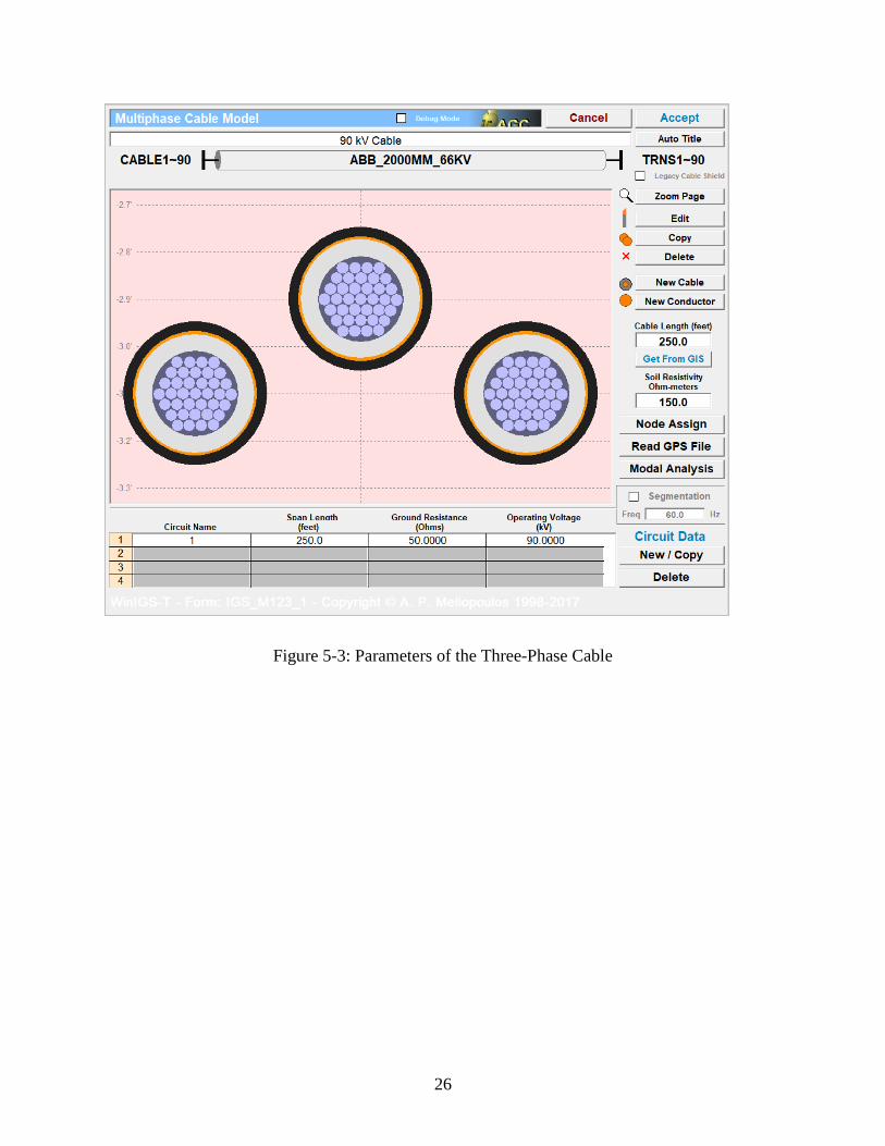
The parameter dialog of the three-phase three-winding transformer and the cable are illustrated in Figure 5-2 and Figure 5-3, respectively. This dialog can be accessed via left button double clicking on the device icon.

25
Figure 5-2: Parameters of the Three-Phase Three-Winding Transformer
26
Figure 5-3: Parameters of the Three-Phase Cable

27
5.1.2 Creating Measurement Models for Merging Units
The instrumentation channel and measurement parameters to be used by the EBP relay for the Protection Zone 1 are modeled in the Merging Unit (see MU icon in Figure 5-1). In this example, three merging units are set up to monitor the phase currents and voltages in the protection zone. The total number of measurements obtained from merging units is 24 at time t. The merging unit model parameters and instrumentation channel list can be edited by clicking on the merging unit icon. This action will bring the user interface illustrated in Figure 5-4. Click on the Instrumentation button to open the instrumentation channel list dialog, illustrated in Figure 5-5. Double-click on each list table entry to inspect the instrumentation channel parameters. Figures 5-6 and 5-7 illustrate examples of a voltage and a current channel, respectively. Note that a WinIGS-T instrumentation channel model includes models of the instrument transformer, instrumentation cable, burdens, and data acquisition device. A short description of the instrumentation channel parameters is presented in Table 5-1.
Figure 5-4: Merging Unit Main Parameter Dialog

28
Figure 5-5: Merging Unit Instrumentation Channel List Dialog
Figure 5-6: Example of a Voltage Instrumentation Channel Dialog

29
Figure 5-7: Example of a Current Instrumentation Channel Dialog

30
Table 5-1: Instrumentation Channel Parameters – User Entry Fields
Parameter Description
Data Type Specifies the type of the measured quantity. Valid options for merging units are Voltage Time Domain Waveform and Current Time Domain Waveform.
Bus Name The bus name where the measurement is taken
Power Device Identifies the power device into which the current is measured (not used for voltage measurements)
Phase The phase of the measured quantity (A, B, C, N, etc.)
Current Direction
The direction of current flow which is considered positive. For example, checking into device indicates that the positive current flow is into the power device terminal (See also Power Device parameter above)
Standard Deviation Quantifies the expected error of the instrumentation channel in per unit of the maximum value that the channel can measure (See also channel scale parameter).
Meter Scale
The maximum peak value that the channel can measure defined at the instrument transformer primary side. Note that this value can be directly entered by the user, or automatically computed from the instrument transformer and data acquisition device characteristics. In order to automatically compute the, click on the Update button located below the Meter Scale field.
Instrument Transformer Code
Name
An identifier of the instrument transformer associated with this channel. Note that WinIGS uses this identifier to generate the channel name. For example, the phase A voltage channel is automatically named V_VT1_AN, if the instrument transformer name is set to VT1.
Instrument Transformer Type
and Tap
Selects instrument transformer parameters from a data library. The library includes parameters needed to create instrument channel models such as turns ratio, frequency response, etc. To select an instrument transformer model, click on the type or tap field to open the instrument transformer data library dialog (See also Figure 5-8)
L-L Nominal Primary Voltage The line to line voltage at the instrument transformer primary side.
Instrumentation Cable Length
The length of the instrumentation cable connecting the instrument transformer secondary with the data acquisition device.
Cable Type The instrumentation cable type and size. Clicking on this field opens the cable library selection window. Note that if the desired cable is not found in the library, a cable library editor is available allowing adding and modifying cable parameters (See WinIGS-T

31
user’s manual for details).
Attenuator Attenuation value of any additional voltage or current reduction divider. Set to 1.0 if none.
Burden The equivalent resistance of the burdens attached to the instrument transformer secondary.
IED
Selects data acquisition device from an IED library. This setting retrieved the data acquisition device frequency response for the purpose of applying error correction. Set to UNITY if this information is not available.
Maximum Peak Value
Set to the maximum instantaneous (peak) voltage or current value that will not saturate the data acquisition device input. This value can be found in data acquisition device specifications. For example, the GE Merging unit voltage and current max peak values can be derived from the voltage and current range specifications shown in Figure 5-9. Note that the range is specified in RMS so these Figures must be multiplied by 2 to obtain the peak values (i.e.: 325.3 Volts and 282.8 Amperes)
Calibration Factor The channel output is multiplied by this value. Set to 1.0 if none required.
Calibration Offset This value is added to the channel output. Set to 0.0 if none required.
Time Skew Time delay in seconds of this channel with respect to time reference. Set to zero for no delay.

32
Figure 5-8: Instrument Transformer Library Dialog

33
Figure 5-9: Example Input Specifications of a GE MU320 Merging Unit

34
Note that the order of the instrumentation channels can be modified using the MoveUp and MoveDown buttons of the instrumentation channel list dialog (Shown in Figure 5-5). Once the instrumentation channel parameter entry is completed, click on the Accept button of the instrumentation channel list dialog, to save the channel parameters. Note that the instrumentation channel parameters are saved in an ASCII file named:
CASENAME_Fnnnnn.ich where CASENAME is the WinIGS-T network model file name root, and nnnnn is a 5-digit integer. These files are stored in the same directory as the WinIGS-T network model file. The next step is to define the measurements to be used for the EBP relay, in terms of the defined instrumentation channels. This is accomplished by clicking on the Measurement button of the merging unit ASDU dialog (Shown in Figure 5-4). This action opens the Measurement List Dialog illustrated in Figure 5-10. For most cases (including the protection zone 1 described in this document), the measurement parameters can be created automatically using the Auto Create button in the Measurement List Dialog.
Figure 5-10: Measurement List Dialog Measurement parameters can be manually created and edited using the New and Edit buttons of the Measurement List dialog (Figure 5-10), which open the measurement parameter dialog illustrated in Figures 5-11 and 5-12. The fields in this dialog are briefly described in Table 5-2.

35
Figure 5-11: Voltage Measurement Parameters Dialog
Figure 5-12: Current Measurement Parameters Dialog

36
Table 5-2: Measurement Parameters – User Entry Fields
Parameter Description
Measurement Formula
Mathematical expression giving measurement value in terms of instrumentation channel values. Note that the measurement formula for automatically created measurements form instrument channels is simply the instrument channel name. However, a measurement can be manually defined as any expression involving all available instrument channels.
Measurement Name
Voltage measurements names are automatically formed based on the bus name, phase and measurement type. For example, a phase A voltage measurement on Bus TRNS1~225 is automatically named V_TRNS1~225_AN. Similarly, current measurements are automatically formed by identifying a power device and a specific terminal into which the measured current is flowing. For example, the phase A current into the transformer at Bus TRNS1~225 is named C_TRNS1~225_TRNS1~90_TRNS1~T_1_TRNS1~225_A, where the part TRNS1~225_TRNS1~90_TRNS1~T_1 identifies the power device as circuit 1 connected to the bus TRNS1~225, and the last part _TRNS1~225 identifies the terminal into which the measured current is flowing. Note that the name part 1 is the user specified Circuit Name of the transformer.
Name at IED
The measurement name as defined by the merging unit or other IED used. The default channel names vary with IED manufacturers and IED types. For example, the GE MU320 merging units default channel names are Ia_1, Ib_1, Ic_1, for the current channels and Va_1, Vb_1, Vc_1, for voltage channels.
IED Channel Order
An order number (starting with 1) indicating the ordering of the channels in the Sample Value packets. For example, GE MU320 merging units SV packets have four current channels followed by four voltage channels. Thus, the current channel order numbers are 1, 2, 3, 4 for phase A, B, C N, and the voltage channel order numbers are 5, 6, 7, and 8 for phases A, B, C, and N.
Merging Unit Scale Factor and
Merging Unit Offset
These values define the conversion from the 32 bit integer Sample Values to actual values in Volts and Amperes. Specifically: Vk = a Xk + b where Vk is a voltage sample in volts, a is the Scale Factor, Xk is the sample value voltage sample (32 bit integer), and b is the Merging Unit Offset. The default merging unit scale factor for voltage channels is 0.01, while for current channels is 0.001. Default offsets are zero.

37
Magnitude Calibration and
Phase Calibration
Measurement magnitude and a phase angle correction value. Default values are 1.0 and 0.0 respectively.
In this example, 3 merging units are placed in this protection zone for estimation based protection. The instrumentation channels of these merging units are listed in Table 5-3. The total number of these channels is 24.
Table 5-3: Instrumentation Channels of Merging Units in Protection Zone 1
MU Name Voltage Channels Current Channels # of
channels of this MU
MU1 AN, BN, CN at TRNS1~225
A, B, C at TRNS1~225 (into the XFMR) 9 A, B, C at TRNS1~T (into
the XFMR)
MU2
AN, BN, CN at TRNS1~90 A, B, C at TRNS1~90 (into
the XFMR) 9 AN, BN, CN at TRNS1~T
MU3 AN, BN, CN at CABLE1~90
A, B, C at CABLE1~90 (into the cable) 6

38
5.1.3 Exporting Measurement and Protection Zone Models
In order to generate the estimation based protective relay files (to be used in the XFM program EBP feature), perform the following steps:
1. Select the power devices belonging to the protection zone of interest. In this example select the transformer, cable, and two breakers in the protection zone 1. (NOTE: to select multiple objects, hold down the CTRL key, and left-click on the elements to be selected).
2. Select the merging units monitoring the voltages and currents to be used in the EBP relay. In this example, select the merging unit named “MU1”, “MU2”, and “MU3” in Figure 5-2. (NOTE: to select multiple objects, hold down the CTRL key, and left-click on the elements to be selected).
3. Execute the SCAQCF Export command of the Tools menu, or click on the toolbar icon:
(See also Figure 5-13).
Figure 5-13: Selecting Zone Power Devices and Merging Units
This command/toolbar button opens the dialog window illustrated in Figure 5-14.

39
Figure 5-14: EBP Export Dialog
4. Click on the entry field under the Export File Path label in order to select the file path of
the files to be generated.
5. Click on the Export button to generate the files. Optionally click on the Report button to verify that the process was completed successfully (See Figure 5-15)
Figure 5-15: Message Window Indicating EBP File Creation Progress & File Paths
The generated files are next used to automatically setup the EBP relay in the XFM program.

40
5.2 Creating Events and Storing in COMTRADE
For the above stated purpose, we use WinIGS-T to define events, simulate the events and store the results in COMTRADE format. Two such events are described below.
5.2.1 Event A: UseCase_01.A
Event A is defined with a phase A to neutral fault at TRNS1~90 bus within the protection zone. Figure 5-16 shows the fault model and fault model parameters dialog. This is a fault occurring inside Zone 1 which should be cleared by opening the two breakers connected to this zone. The fault is initiated at 0.5 seconds from the start of the simulation.
Figure 5-16: Network Model with Fault between Phase A and Neutral at Bus TRNS1~90
The simulation is executed for a period of one second. The measurements generated during the simulation are stored in a COMTRADE file. Figure 5-17 shows the time domain simulation parameters dialog where the simulation time step, duration, as well as the COMTRADE output is specified. Note that the time step is selected to match the standard merging unit sampling rate at 80 samples per cycle. For a 50 Hz system this is achieved by selecting the time step at: Δt = 1,000,000 / ( 50 x 80 ) = 250 microseconds. The voltages and currents captured by the three merging units are plotted in Figure 5-18 to Figure 5-20. The WinIGS-T case files is named RTE_PZone1_EVENT_A.NMT and is provided with this report. The generated COMTRADE configuration and data files are named RTE_PZone1_EVENT_A_BLOCX.cfg and RTE_PZone1_EVENT_A_BLOCX.dat respectively.

41
Figure 5-17: Time Domain Simulation Parameters Dialog

42
Figure 5-18: Voltage and Current Measurements Obtained from Merging Unit 1 in Event A
-195
-93
9
112
214kV
V_TRNS1~225_ANV_TRNS1~225_BNV_TRNS1~225_CN
195.5 kV (peak) 188.5 kV (peak) 194.4 kV (peak)
-0.973
-0.494
-0.016
0.463
0.941
kA
C_TRNS1~225_TRNS1~90_TRNS1~T_1_TRNS1~225_AC_TRNS1~225_TRNS1~90_TRNS1~T_1_TRNS1~225_BC_TRNS1~225_TRNS1~90_TRNS1~T_1_TRNS1~225_C
957.0 A (peak) 82.15 A (peak) 98.85 A (peak)
-0.107
-0.053
0.002
0.056
0.110
A
C_TRNS1~225_TRNS1~90_TRNS1~T_1_TRNS1~T_AC_TRNS1~225_TRNS1~90_TRNS1~T_1_TRNS1~T_BC_TRNS1~225_TRNS1~90_TRNS1~T_1_TRNS1~T_C
104.8 mA (peak) 105.7 mA (peak) 107.1 mA (peak)
0.000 0.167 0.333 0.500 0.667 0.833 1.000Time (Seconds)

43
Figure 5-19: Voltage and Current Measurements Obtained from Merging Unit 2 in Event A
-77.8
-35.6
6.6
48.8
91.0kV
V_TRNS1~90_ANV_TRNS1~90_BNV_TRNS1~90_CN
80.84 kV (peak) 74.89 kV (peak) 77.46 kV (peak)
-2.36
-1.16
0.04
1.24
2.44
kA
C_TRNS1~225_TRNS1~90_TRNS1~T_1_TRNS1~90_AC_TRNS1~225_TRNS1~90_TRNS1~T_1_TRNS1~90_BC_TRNS1~225_TRNS1~90_TRNS1~T_1_TRNS1~90_C
2.395 kA (peak) 209.9 A (peak) 233.0 A (peak)
-8.14
-3.45
1.23
5.92
10.60
kV
V_TRNS1~T_ANV_TRNS1~T_BNV_TRNS1~T_CN
9.370 kV (peak) 8.126 kV (peak) 8.134 kV (peak)
0.000 0.167 0.333 0.500 0.667 0.833 1.000Time (Seconds)

44
Figure 5-20: Voltage and Current Measurements Obtained from Merging Unit 3 in Event A
-77.8
-35.6
6.6
48.8
91.0kV
V_CABLE1~90_ANV_CABLE1~90_BNV_CABLE1~90_CN
80.83 kV (peak) 74.89 kV (peak) 77.46 kV (peak)
-4.70
-2.37
-0.05
2.28
4.60
kA
C_CABLE1~90_TRNS1~90_1_CABLE1~90_AC_CABLE1~90_TRNS1~90_1_CABLE1~90_BC_CABLE1~90_TRNS1~90_1_CABLE1~90_C
4.650 kA (peak) 209.8 A (peak) 234.5 A (peak)
0.000 0.167 0.333 0.500 0.667 0.833 1.000Time (Seconds)

45
5.2.2 Event B: UseCase_01.B
Event B is defined as a phase A to neutral fault at bus A225D2 (an external fault). Figure 5-21 shows the fault model and fault model parameters dialog. This is a fault occurring outside protection zone 1 and therefore the breakers of zone 1 should not operate. The fault is initiated at 0.5 seconds from the start of the simulation and lasts 0.1 second.
Figure 5-21: Network Model with Fault between Phase A and Neutral at Bus A225D2
The simulation is executed for a period of one second. The measurements generated during the simulation are stored in a COMTRADE file. The time step is selected to match the standard merging unit sampling rate at 80 samples per cycle, which for a 50 Hz system is 250 microseconds (i.e. same as for Event A). The voltages and currents captured by the three merging units are plotted from Figure 5-22 to Figure 5-24. The WinIGS-T case file is named as RTE_PZone1_EVENT_B.NMT and is provided with this report. The generated COMTRADE configuration and data files are named RTE_PZone1_EVENT_B_BLOCX.cfg and RTE_PZone1_EVENT_B_BLOCX.dat, respectively.

46
Figure 5-22: Voltage and Current Measurements Obtained from Merging Unit 1 in Event B
-206
-101
4
109
214kV
V_TRNS1~225_ANV_TRNS1~225_BNV_TRNS1~225_CN
195.8 kV (peak) 198.3 kV (peak) 204.6 kV (peak)
-105.6
-52.6
0.4
53.4
106.4
A
C_TRNS1~225_TRNS1~90_TRNS1~T_1_TRNS1~225_AC_TRNS1~225_TRNS1~90_TRNS1~T_1_TRNS1~225_BC_TRNS1~225_TRNS1~90_TRNS1~T_1_TRNS1~225_C
90.81 A (peak) 84.25 A (peak) 106.0 A (peak)
-0.107
-0.053
0.002
0.056
0.110
A
C_TRNS1~225_TRNS1~90_TRNS1~T_1_TRNS1~T_AC_TRNS1~225_TRNS1~90_TRNS1~T_1_TRNS1~T_BC_TRNS1~225_TRNS1~90_TRNS1~T_1_TRNS1~T_C
104.8 mA (peak) 105.7 mA (peak) 107.1 mA (peak)
0.000 0.167 0.333 0.500 0.667 0.833 1.000Time (Seconds)

47
Figure 5-23: Voltage and Current Measurements Obtained from Merging Unit 2 in Event B
-81.7
-38.5
4.7
47.8
91.0kV
V_TRNS1~90_ANV_TRNS1~90_BNV_TRNS1~90_CN
80.91 kV (peak) 78.62 kV (peak) 81.40 kV (peak)
-247
-124
-0
123
247
A
C_TRNS1~225_TRNS1~90_TRNS1~T_1_TRNS1~90_AC_TRNS1~225_TRNS1~90_TRNS1~T_1_TRNS1~90_BC_TRNS1~225_TRNS1~90_TRNS1~T_1_TRNS1~90_C
219.1 A (peak) 218.2 A (peak) 247.0 A (peak)
-8.15
-3.46
1.23
5.91
10.60
kV
V_TRNS1~T_ANV_TRNS1~T_BNV_TRNS1~T_CN
9.378 kV (peak) 8.126 kV (peak) 8.134 kV (peak)
0.000 0.167 0.333 0.500 0.667 0.833 1.000Time (Seconds)

48
Figure 5-24: Voltage and Current Measurements Obtained from Merging Unit 3 in Event B
-81.7
-38.5
4.7
47.8
91.0kV
V_CABLE1~90_ANV_CABLE1~90_BNV_CABLE1~90_CN
80.91 kV (peak) 78.62 kV (peak) 81.40 kV (peak)
-247
-124
-0
123
247
A
C_CABLE1~90_TRNS1~90_1_CABLE1~90_AC_CABLE1~90_TRNS1~90_1_CABLE1~90_BC_CABLE1~90_TRNS1~90_1_CABLE1~90_C
215.8 A (peak) 218.4 A (peak) 247.1 A (peak)
0.000 0.167 0.333 0.500 0.667 0.833 1.000Time (Seconds)

49
5.3 EBP Results
This section presents the results obtained from the EBP relay for the use case and events described in Section 5.2. The EBP relay has been implemented within the WinXFM Program. In order to setup the EBP relay and run the use cases, execute the WinXFM program, open one of the provided WinXFM files, and click on the EBP button as indicated in Figure 5-25.
Figure 5-25: Opening the EBP Main Setup Form in the WinXFM Program
5.3.1 Event A: UseCase_01.A
As described in Section 5.2, Event A is defined as a phase A to neutral fault at bus TRNS1~90. To run the EBP relay using the Event A data, execute the WinXFM program and open the WinXFM file:
RTE-SYSTEM-B-EVENT-A
Note: this file is provided with this report under the file name RTE-SYSTEM-B-EVENT-A.xfm Click on the Import button of the main EBP dialog window to open the “Device and Measurement File” dialog shown in Figure 5-25. Verify that the Zone_1 Device and Measurement files have been selected and that the model domain and model kind are selected as “Time Domain” and “Algebraic Companion Form”. Click on the Import button, and verify that the selected protection zone devices are listed and the active column is checked as illustrated in Figure 5-26. Click on the Accept button to close the Device and Measurement File dialog. This procedure imports the measurement definition and device model data generated using the WinIGS-T program and stored in the data files:
• PZone1.TDMDEF (Measurement Definition File)

50
• PZone1.TDSCAQCF (Device Model File)
Figure 5-26: Importing Zone 1 Device and Measurement Definition Files
Next click on the Setup button of the COMTRADE Data block of the main EBP dialog (See Figure 5-27) to open the COMTRADE Data Playback dialog (shown in Figure 5-28). Verify that the COMTRADE File Name field indicating the Event A waveform data has been selected: (file name: RTE_PZone1_EVENT_A_BLOCX). Also verify the following:
• Playback rate is set at 4000 samples per second for 50 Hz systems.
• Speed Factor radio button is selected and the speed factor is set to 5.0. The speed factor option allows the relay response to be observed in slow motion. Otherwise, if you select the real-time option, the playback will occur in real time and the whole process will be completed in one second, i.e., the duration of the waveform data stored in the COMTRADE file. Click on the Close button to close the COMTRADE Data Playback dialog.

51
Figure 5-27: Opening the COMTRADE Setup Dialog
Figure 5-28: Selecting the COMTRADE Data Files for Playback

52
At this point, the system is ready to execute the EBP relay using the Event A data. It is recommended to click on the Save ( ) button of the main WinXFM user interface (Horizontal Tool-Bar) in order to save all entered setup parameters. Click on the Start button of the EBP Relay block to start the EBP relay, then on the Start button of the COMTRADE Data block to start streaming the data to the relay. The performance metrics of this event is illustrated in Figure 5-29. Note that the confidence level is 100% before the fault, and reaches to zero immediately upon the fault initiation. The trip decision is then made within a certain delay that can be determined by clicking the Relay Settings button in Figure 5-27. In addition to the channels shown in Figure 5-29, a list of available channels for plotting is shown in Figure 5-30. This can be achieved by clicking on the Select Channels to Display ( ) button in the main WinXFM user interface (Horizontal Tool Bar).
Figure 5-29: Plots of Some Actual/Estimated Measurements, Residuals, Confidence Level, and
Trip Decision in Event A

53
Figure 5-30: A List of Available Channels for Plotting

54
5.3.2 Event B: UseCase_01.B
Event B is defined as a phase A to neutral fault at bus A225D2 (an external fault). To run the EBP relay using the Event B simulated waveforms, execute the WinXFM program and open the WinXFM file:
RTE-SYSTEM-B-EVENT-B
Note: this file is provided with this report under the file name RTE-SYSTEM-B-EVENT-B.xfm Click on the Import button of the main EBP dialog window to open the “Device and Measurement Files” dialog shown in Figure 5-31. Verify that the Zone_1 Device and Measurement files have been selected and that the model domain and model kind are selected as “Time Domain” and “Algebraic Companion Form”. Click on the Import button, and verify that the selected protection zone devices are listed and the active column is checked as illustrated in Figure 5-31. Click on the Accept button to close the Device and Measurement Files dialog. This procedure imports the measurement definition and device model data generated using the WinIGS-T program and stored in the data files:
• PZone1.TDMDEF (Measurement Definition File)
• PZone1.TDSCAQCF (Device Model File)

55
Figure 5-31: Importing Zone 1 Device and Measurement Definition Files
Next click on the Setup button of the COMTRADE Data block of the main EBP dialog (See Figure 5-32) to open the COMTRADE Data Playback dialog (shown in Figure 5-33).

56
Figure 5-32: Opening the COMTRADE Setup Dialog
Verify that the COMTRADE File Name field indicates that the Event B waveform data has been selected: (file name: RTE_PZone1_EVENT_B_BLOCX). Also verify the following:
• Playback rate is set at 4000 samples per second for 50 Hz systems.
• Speed Factor radio button is selected and the speed factor is set to 5.0. The speed factor option allows the relay response to be observed in slow motion. Otherwise, if you select the real-time option, the playback will occur in real time and the whole process will be completed in one second, i.e., the duration of the waveform data stored in the COMTRADE file. Click on the Close button to close the COMTRADE Data Playback dialog.

57
Figure 5-33: Selecting the COMTRADE Data files for Playback
At this point, the system is ready to execute the EBP relay using the Event B data. It is recommended to click on the Save ( ) button of the main WinXFM user interface (Horizontal Tool-Bar) in order to save any modified setup parameters. Click on the Start button of the EBP Relay block to start the EBP relay, then on the Start button of the COMTRADE Data block to start streaming the data to the relay. The performance metrics of this event is illustrated in Figure 5-34. Note that the confidence level is nearly 100% before the fault, as well as during the fault. Only small spikes occur when the fault is initiated and ended. Note that the breakers remain closed (as expected) during the whole event since the fault is outside the protection zone. In addition to the channels shown in Figure 5-34, a list of available channels for plotting is shown in Figure 5-35. This can be achieved by clicking on the Select Channels to Display ( ) button in the main WinXFM user interface (Horizontal Tool Bar).

58
Figure 5-34: Plots of Some Actual/Estimated Measurements, Residuals, Confidence Level, and
Trip Decision in Event B

59
Figure 5-35: A List of Available Channels for Plotting

60
6. Example Test Results: RTE Protection Zone 04
This section describes a use case for preparing and running the setting-less relay for the specific protection zone 4 of the RTE substation BLOCX. Protection Zone 4 is a shunt reactor bank at the 225 kV section of the BLOCKX substation. The inductor bank is connected to breaker and a main/transfer bus arrangement. First, the protection zone model is developed in the program WinIGS-T. Once the protection zone model has been defined, it is exported into two files that are readable by the Estimation Based Protection (EBP) program. The first file contains the model of the protection zone power components. Note that a protection zone may include one or more components, for example protection zone 4 contains a reactor and breakers. Each protection zone component model is represented in its SCPAQCF format (State, Control, and Parameter Algebraic Quadratic Companion Form). The second file contains the definition of the measurements. The measurements definition provides the IED (Merging unit providing the measurement, type of measurement, and where on the protection zone the measurement was taken. The measurement definition is key-word oriented. A number of events have been simulated with the program WinIGS-T, using the RTE BLOCAUX substation model. The results of the simulation provided by the merging units of the Protection Zone 4 are stored in COMTRADE format. These files are used for playback through a series of conversions and amplifiers into merging units connected to the EBP relay in the laboratory. The use case demonstrates the EBP procedure consisting of the following steps:
• Read model and measurement files
• Read event data (COMTRADE files)
• Run the setting-less relay. This report includes several simulated events as well as the EBP results.

61
6.1 Creating Protection Zone Models for EBP Relays
WinIGS-T includes a tool which automatically generates the model of the user selected protection zone in the SCPAQCF syntax. The protection zone can be a single component protection zone or it may comprise several components and/or breakers. The estimation based protective relay (EBP, a.k.a. setting-less relay) requires the model of the protection zone in SCPAQCF standard. The user should select the components that constitute the protection zone and which must be exported in the SCPAQCF syntax into a file. In addition, the user must specify the merging units providing data to the EBP relay in order to generate a second file describing the measurement parameters. These two files are read by the WinXFM-EBP program which executes the estimation based protective relay algorithm.
6.1.1 Creating the Network Time Domain Model
The procedure to generate the EBP model file begins by building a system model in WinIGS-T. The WinIGS-T model could include the entire or part of the large system (for simulation studies and for generating events) and must also include the models of the protection zone under study. Specifically:
• The power devices comprising the EBP protection zone.
• The instrumentation channels available to the EBP relay via merging units.
• The breakers/switches that enable the protection of the zone. The WinIGS-T model for the RTE system, including the necessary merging unit information is provided along with this document. The RTE network model is shown in Figure 6-1. Note that the RTE substation of interest is represented by the circular icon labelled SUB BLOCKX. Double click on this icon to open the substation single line diagram view, illustrated in Figure 6-2. Next zoom in to view the protection zone if interest i.e. Protection Zone 4, containing a 3-Phase shunt reactor bank and a breaker. The diagram also includes a Merging Unit which captures the reactor voltages and currents.

62
Figure 6-1: RTE System Network Model

63
Figure 6-2: RTE Substation Single Line Diagram (top) and Protection Zone 04 (bottom)

64
The parameters dialog of the shunt inductor bank is illustrated in Figure 6-3. This dialog can be accessed via left button double clicking on the inductor icon. Note that the model parameters are typical nameplate information such as rated voltage and reactive power. Ensure that the reactor model parameters are correctly set. The magnetizing current of the inductor are calculated by a non-linear function in terms of the flux through the core.
Figure 6-3: Protection Zone 4 Parameters

65
6.1.2 Creating Measurement Models for Merging Units
The instrumentation channel and measurement parameters to be used by the EBP relay for the Zone 4 Protection are modeled in the Merging Unit (see MU icon in Figure 6-2). In this example the EBP relay monitors the phase currents and voltages at the reactor bank terminals. The merging unit model parameters and instrumentation channel list can be edited by clicking on the merging unit icon. This action will bring the user interface illustrated in Figure 6-4. Click on the Instrumentation button to open the instrumentation channel list dialog, illustrated in Figure 6-5. Double-click on each list table entry to inspect the instrumentation channel parameters. Figures 6-6 and 6-7 illustrate examples of a voltage and a current channel respectively. Note that a WinIGS-T instrumentation channel model includes models of the instrument transformer, instrumentation cable, burdens, and data acquisition device (i.e. a merging unit in these example). A short description of the instrumentation channel parameters is presented in TABLE 6-1.
Figure 6-4: Merging Unit Main Parameter Dialog

66
Figure 6-5: Merging Unit Instrumentation Channel List Dialog
Figure 6-6: Example of a Voltage Instrumentation Channel Dialog

67
Figure 6-7: Example of a Current Instrumentation Channel Dialog

68
Table 6-1: Instrumentation Channel Parameters – User Entry Fields
Parameter Description
Data Type Specifies the type of the measured quantity. Valid options for merging units are Voltage Time Domain Waveform and Current Time Domain Waveform.
Bus Name The bus name where the measurement is taken
Power Device Identifies the power device into which the current is measured (not used for voltage measurements)
Phase The phase of the measured quantity (A, B, C, N, etc.)
Current Direction The direction of current flow which is considered positive. For example, checking into device indicates that the positive current flow is into the power device terminal (See also Power Device parameter above)
Standard Deviation Quantifies the expected error of the instrumentation channel in per unit of the maximum value that the channel can measure (See also channel scale parameter).
Meter Scale The maximum peak value that the channel can measure defined at the instrument transformer primary side. Note that this value can be directly entered by the user, or automatically computed from the instrument transformer and data acquisition device characteristics. In order to automatically compute the ,click on the Update button located below the Meter Scale field.
Instrument Transformer Code
Name
An identifier of the instrument transformer associated with this channel. Note that WinIGS uses this identifier to generate the channel name. For example the phase A voltage channel is automatically named V_REACTOR_AN, if the instrument transformer name is set to REACTOR.
Instrument Transformer Type
and Tap
Selects instrument transformer parameters from a data library. The library includes parameters needed to create instrument channel models such as turns ratio, frequency response, etc. To select an instrument transformer model, click on the type or tap field to open the instrument transformer data library dialog (See also Figure 6-8)
L-L Nominal Primary Voltage
The line to line voltage at the instrument transformer primary side.
Instrumentation Cable Length
The length of the instrumentation cable connecting the instrument transformer secondary with the data acquisition device.
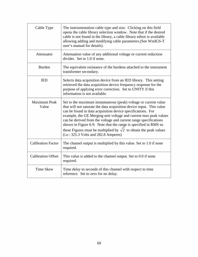
69
Cable Type The instrumentation cable type and size. Clicking on this field opens the cable library selection window. Note that if the desired cable is not found in the library, a cable library editor is available allowing adding and modifying cable parameters.(See WinIGS-T user’s manual for details).
Attenuator Attenuation value of any additional voltage or current reduction divider. Set to 1.0 if none.
Burden The equivalent resistance of the burdens attached to the instrument transformer secondary.
IED Selects data acquisition device from an IED library. This setting retrieved the data acquisition device frequency response for the purpose of applying error correction. Set to UNITY if this information is not available.
Maximum Peak Value
Set to the maximum instantaneous (peak) voltage or current value that will not saturate the data acquisition device input. This value can be found in data acquisition device specifications. For example, the GE Merging unit voltage and current max peak values can be derived from the voltage and current range specifications shown in Figure 6-9. Note that the range is specified in RMS so these Figures must be multiplied by 2 to obtain the peak values (i.e.: 325.3 Volts and 282.8 Amperes)
Calibration Factor The channel output is multiplied by this value. Set to 1.0 if none required.
Calibration Offset This value is added to the channel output. Set to 0.0 if none required.
Time Skew Time delay in seconds of this channel with respect to time reference. Set to zero for no delay.

70
Figure 6-8: Instrument Transformer Library Dialog

71
Figure 6-9: Example Input Specifications of A GE MU320 Merging Unit

72
Note that the order of the instrumentation channels can be modified using the MoveUp and MoveDown buttons of the instrumentation channel list dialog (Shown in Figure 6-5). Once the instrumentation channel parameter entry is completed, click on the Accept button of the instrumentation channel list dialog, to save the channel parameters. Note that the instrumentation channel parameters are saved in an ASCII file named:
CASENAME_Fnnnnn.ich where CASENAME is the WinIGS-T network model file name root, and nnnnn is a 5-digit integer. These files are stored in the same directory as the WinIGS-T network model file. The next step is to define the measurements to be used for the EBP relay, in terms of the defined instrumentation channels. This is accomplished by clicking on the Measurement button of the merging unit ASDU dialog (Shown in Figure 6-4). This action opens the Measurement List Dialog illustrated in Figure 6-10. For most cases (including the protection zone 4 described in this document) the measurement parameters can be created automatically using the Auto Create button if the Measurement List Dialog.
Figure 6-10: Measurement List Dialog
Measurement parameters can be manually created and edited using the New and Edit buttons of the Measurement List dialog (Figure 6-10), which open the measurement parameter dialog illustrated in Figures 6-11 and 6-12. The fields in this dialog are briefly described in Table 6-2.

73
Figure 6-11: Voltage Measurement Parameters Dialog
Figure 6-12: Current Measurement Parameters Dialog

74
Table 6-2: Measurement Parameters – User Entry Fields
Parameter Description
Measurement Formula
Mathematical expression giving measurement value in terms of instrumentation channel values. Note that the measurement formula for automatically created measurements form instrument channels is simply the instrument channel name. However, a measurement can be manually defined as any expression involving all available instrument channels.
Measurement Name
Voltage measurements names are automatically formed based on the bus name, phase and measurement type. For example, a phase A voltage measurement on Bus REACTOR is automatically named V_REACTOR_A. Similarly, current measurements are automatically formed by identifying a power device and a specific terminal into which the measured current is flowing. For example, the phase A current into the shunt reactor connected to bus reactor is named C_REACTOR_R1_REACTOR_A, where the part REACTOR_R1 identifies the power device as circuit the R1 connected to the bus REACTOR, and the last part _REACTOR_A identifies the terminal into which the measured current is flowing. Note that the name part R1 is the user specified Circuit Name of the reactor connected at bus REACTOR.
Name at IED The measurement name as defined by the merging unit or other IED used. The default channel names vary with IED manufacturers and IED types. For example the GE MU320 merging units default channel names are Ia_1, Ib_1, Ic_1, ... for the current channels and Va_1, Vb_1, Vc_1, ... for voltage channels.
IED Channel Order
An order number (starting with 1) indicating the ordering of the channels in the Sample Value packets. For example GE MU320 merging units SV packets have four current channels followed by four voltage channels. Thus the current channel order numbers are 1, 2, 3, 4 for phase A, B, C N, and the voltage channel order numbers are 5, 6, 7, and 8 for phases A, B, C, and N.
Merging Unit Scale Factor and
Merging Unit Offset
These values define the conversion from the 32 bit integer Sample Values to actual values in Volts and Amperes. Specifically:
Vk = a Xk + b where Vk is a voltage sample in volts, a is the Scale Factor, Xk is the sample value voltage sample (32 bit integer), and b is the Merging Unit Offset. The default merging unit scale factor for voltage channels is 0.01, while for current channels is 0.001. Default offsets are zero.

75
Magnitude Calibration and
Phase Calibration
Measurement magnitude and a phase angle correction value. Default values are 1.0 and 0.0 respectively.

76
6.1.3 Exporting Measurement and Protection Zone Models
In order to generate the estimation based protective relay files (to be used in the XFM program EBP feature), perform the following steps:
6. Select the power devices belonging to the protection zone of interest. In this example select the shunt reactor bank connected to bus REACTOR and also the breaker connected in series with the shunt reactor bank. (NOTE: to select multiple objects, hold down the CTRL key, and left-click on the elements to be selected).
7. Select the merging units monitoring the voltages and currents to be used in the EBP relay. In this example select the merging unit named “Reactor Merging Unit” in Figure 6-2. (NOTE: to select multiple objects, hold down the CTRL key, and left-click on the elements to be selected).
8. Execute the SCAQCF Export command of the Tools menu, or click on the toolbar icon:
(See also Figure 6-13)
Figure 6-13: Selecting Zone Power Devices and Merging Units
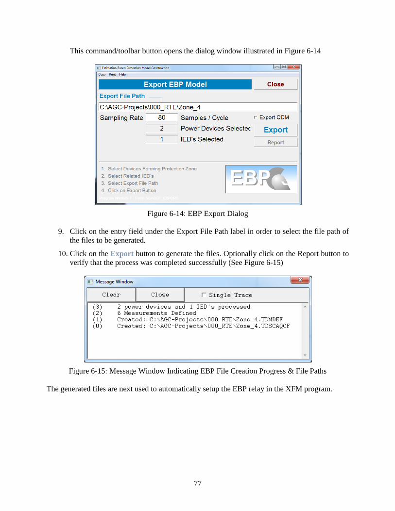
77
This command/toolbar button opens the dialog window illustrated in Figure 6-14
Figure 6-14: EBP Export Dialog
9. Click on the entry field under the Export File Path label in order to select the file path of
the files to be generated.
10. Click on the Export button to generate the files. Optionally click on the Report button to verify that the process was completed successfully (See Figure 6-15)
Figure 6-15: Message Window Indicating EBP File Creation Progress & File Paths
The generated files are next used to automatically setup the EBP relay in the XFM program.

78
6.2 Creating Events and Storing in COMTRADE
For the above stated purpose, we use WinIGS-T to define events, simulate the events and store the results in COMTRADE format. Two such events are described below.
6.2.1 Event A: UseCase_01.A
Event A is defined with a Phase A to neutral fault on the REACTOR bus within the protection zone. Figure 6-16 shows the fault model and fault model parameters dialog. This is a fault occurring inside Zone 4 which should be cleared by opening the reactor breaker. The fault is initiated at 0.5 seconds from the start of the simulation.
Figure 6-16: Network Model with Fault between Phase A and Neutral of REACTOR Bus The simulation is executed for a period of one second. The measurements generated during the simulation are stored in a COMTRADE file. Figure 6-17 shows the time domain simulation parameters dialog where the simulation time step, duration, as well as the COMTRADE output is specified. Note that the time step is selected to match the standard merging unit sampling rate at 80 samples per cycle. For 50 Hz system this is achieved by selecting the time step at:
Δt = 1.000.000 / ( 50 x 80 ) = 250 microseconds. The voltages and currents captured by the reactor bank merging unit are plotted in Figure 6-18.
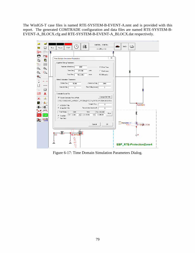
79
The WinIGS-T case files is named RTE-SYSTEM-B-EVENT-A.nmt and is provided with this report. The generated COMTRADE configuration and data files are named RTE-SYSTEM-B-EVENT-A_BLOCX.cfg and RTE-SYSTEM-B-EVENT-A_BLOCX.dat respectively.
Figure 6-17: Time Domain Simulation Parameters Dialog.

80
Figure 6-18: Time Domain Simulation Output Plot for Event A
-245
-105
35
174
kVV_B~REACTOR_AN209.3 kV (peak)
-197 -65
66 198
kV
V_B~REACTOR_BN197.3 kV (peak)
-204 -68
67 202
kV
V_B~REACTOR_CN200.2 kV (peak)
-4.18 -1.60 0.99 3.57
kA
C_B~REACTOR_2_B~REACTOR_A3.877 kA (peak)
-373 42
457 872
A
C_B~REACTOR_2_B~REACTOR_B388.5 A (peak)
-0.859-0.435
-0.011 0.412
kA
C_B~REACTOR_2_B~REACTOR_C428.2 A (peak)
0.213 0.345 0.476 0.607 0.738 0.869 1.000Time (Seconds)

81
6.2.2 Event B: UseCase_01.B
Event B is defined a Phase A to neutral fault on the bus A225D2. Figure 6-19 shows the fault model and fault model parameters dialog. This is a fault occurring outside Zone 4 and therefore the reactor breaker should not operate. The fault is initiated at 0.5 seconds from the start of the simulation and lasts 0.2 seconds.
Figure 6-19: Network Model with Fault between Phase A and Neutral of Bus A225D2. The simulation is executed for a period of one second. The measurements generated during the simulation are stored in a COMTRADE file. The time step is selected to match the standard merging unit sampling rate at 80 samples per cycle, which for a 50 Hz system is 250 microseconds (i.e. same as for Event A). The voltages and currents captured by the reactor bank merging unit are plotted in Figure 6-20 The WinIGS-T case files is named RTE-SYSTEM-B-EVENT-B.nmt and is provided with this report. The generated COMTRADE configuration and data files are named RTE-SYSTEM-B-EVENT-B_BLOCX.cfg and RTE-SYSTEM-B-EVENT-B_BLOCX.dat respectively.

82
Figure 6-20: Time Domain Simulation Output Plot for Event B
-245
-105
35
174
kVV_B~REACTOR_AN209.6 kV (peak)
-197 -66
66 197
kV
V_B~REACTOR_BN197.2 kV (peak)
-202 -67
67 202
kV
V_B~REACTOR_CN202.2 kV (peak)
-351 -137 77 291
A
C_B~REACTOR_2_B~REACTOR_A321.2 A (peak)
-373 -114
145 404
A
C_B~REACTOR_2_B~REACTOR_B388.5 A (peak)
-454 -165
123 412
A
C_B~REACTOR_2_B~REACTOR_C432.9 A (peak)
0.302 0.418 0.534 0.650 0.767 0.883 0.999Time (Seconds)

83
6.3 EBP Results
This section presents the results obtained with the EBP relay for the use case and events described in Section 6.2. The EBP relay has been implemented within the WinXFM Program. In order to setup the EBP relay to run the use cases, execute the WinXFM program, open one of the provided WinXFM files, and click on the EBP button as indicated in Figure 6-21.
Figure 6-21: Opening the EBP Main Setup Form in the WinXFM Program
6.3.1 Event a: UseCase_01.A
As described in Section 6.2, event A is defined as a Phase A to neutral fault on the REACTOR bus. To run the EBP relay using the Event A data, execute the WinXFM program and open the WinXFM file:
RTE-SYSTEM-B-EVENT-A
Note: this file is provided with this report under the file name RTE-SYSTEM-B-EVENT-A.xfm Click on the Import button of the main EBP dialog window to open the “Device and Measurement File” dialog shown in Figure 6-22. Verify that the Zone_4 Device and Measurement files have been selected and that the two checkboxes titled Time Domain and Algebraic Companion Form are checked. Click on the Import button, and verify that the selected protection zone devices are listed and the active column is checked as illustrated in Figure 6-22. Click on the Accept button to close the Device and Measurement File dialog. This procedure imports the measurement definition and device model data generated using the WinIGS-T program and stored in the data files:

84
• Zone_4.TDMDEF (Measurement Definition File) • Zone_4.TDSCAQCF (Device Model File)
Figure 6-22: Importing Zone 4 Device and Measurement Definition Files Next click on the Setup button of the COMTRADE Data block of the main EBP dialog (See Figure 6-23) to open the COMTRADE Data Playback dialog (shown in Figure 6-24). Verify that the COMTRADE File Name field indicates that the Event A waveform data has been selected: (file name: RTE-SYSTEM-B-EVENT-A_BLOCX). Also verify the following:
• Playback rate is set at 4000 samples per second for 50 Hz systems.
• Speed Factor radio button is selected and the speed factor is set to 20.0. The speed factor option allows the relay response to be observed in slow motion. Otherwise, if you select the real time option, the playback will occur in real time and the whole process will be completed in one second i.e. the duration of the waveform data stored in the COMTRADE file. Click on the Close button to close the COMTRADE Data Playback dialog.

85
Figure 6-23: Opening the COMTRADE Setup Dialog
Figure 6-24: Selecting the COMTRADE Data files for Playback

86
At this point, the system is ready to execute the EBP relay using the Event A data. It is
recommended to click on the Save ( ) button of the main WinXFM user interface (Horizontal Tool-Bar) in order to save all entered setup parameters. Click on the Start button of the EBP Relay block to start the EBP relay, then Click on the Start button of the COMTRADE Data block. (See Figure 6-25 for the location of these buttons).
Figure 6-25: Starting the EBP Relay Using Playback Data (COMTRADE)
A number of plots can be viewed on the main WinXFM user interface such as measured and estimated values trip decision etc. An example of such plots is given in Figure 6-26. A list of the available channels for plotting is shown in Figure 6-27. Note that the confidence level is nearly 100% before the fault, and reaches to almost zero immediately upon the fault initiation.

87
Figure 6-26: Plots of Measurement and Estimated Values, Confidence Level and Trip Decision
during Event A
3541.3 A
-4183.1 A
Actual_Inst_Current_B~REACTOR_A (A)Est_Meas_Actual_Inst_Current_B~REACTOR_A (A)
975.7 kV
-1922.2 kV
Actual_Inst_Voltage_B~REACTOR_A_B~REACTOR_N (V)Est_Meas_Actual_Inst_Voltage_B~REACTOR_A_B~REACTOR_N
100.00
0.000
Confidence_Level
1.000
0.000
Trip_Decision
0.378 s 0.589 s

88
Figure 6-27: Available Data for Plotting on the Main WinXFM Window

89
6.3.2 Event b: UseCase_01.B
Event B is defined as a Phase A to neutral fault on bus A225D2. To run the EBP relay using the Event B simulated waveforms, execute the WinXFM program and open the WinXFM file:
RTE-SYSTEM-B-EVENT-B Note: this file is provided with this report under the file name RTE-SYSTEM-B-EVENT-B.xfm Click on the Import button of the main EBP dialog window to open the “Device and Measurement File” dialog shown in Figure 6-28. Verify that the Zone_4 Device and Measurement files have been selected and that the two checkboxes titled TDSCAQCF and TDMDEF are checked. Click on the Import button, and verify that the selected protection zone devices are listed and the active column is checked as illustrated in Figure 6-28. Click on the Accept button to close the Device and Measurement File dialog. This procedure imports the measurement definition and device model data generated using the WinIGS-T program and stored in the data files:
• Zone_4.TDMDEF (Measurement Definition File)
• Zone_4.TDSCAQCF (Device Model File)
Figure 6-28: Importing Zone 4 Device and Measurement Definition Files

90
Next click on the Setup button of the COMTRADE Data block of the main EBP dialog (See Figure 6-29) to open the COMTRADE Data Playback dialog (shown in Figure 6-30).
Figure 6-29: Opening the COMTRADE Setup Dialog
Verify that the COMTRADE File Name field indicates that the Event B waveform data has been selected: (file name: RTE-SYSTEM-B-EVENT-B_BLOCX). Also verify the following:
• Playback rate is set at 4000 samples per second for 50 Hz systems.
• Speed Factor radio button is selected and the speed factor is set to 20.0. The speed factor option allows the relay response to be observed in slow motion. Otherwise, if you select the real time option, the playback will occur in real time and the whole process will be completed in one second i.e. the duration of the waveform data stored in the COMTRADE file. Click on the Close button to close the COMTRADE Data Playback dialog.

91
Figure 6-30: Selecting the COMTRADE Data Files for Playback
At this point, the system is ready to execute the EBP relay using the Event B data. It is recommended to click on the Save ( ) button of the main WinXFM user interface (Horizontal Tool-Bar) in order to save any modified setup parameters. Click on the Start button of the EBP Relay block to start the EBP relay, then Click on the Start button of the COMTRADE Data block. (See Figure 6-31 for the location of these buttons).
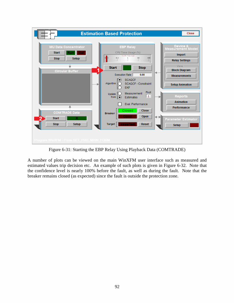
92
Figure 6-31: Starting the EBP Relay Using Playback Data (COMTRADE)
A number of plots can be viewed on the main WinXFM user interface such as measured and estimated values trip decision etc. An example of such plots is given in Figure 6-32. Note that the confidence level is nearly 100% before the fault, as well as during the fault. Note that the breaker remains closed (as expected) since the fault is outside the protection zone.

93
Figure 6-32: Plots of Measurement and Estimated Values, Confidence Level and Trip Decision
during Event B
292.3 A
-360.7 A
Actual_Inst_Current_B~REACTOR_A (A)Est_Meas_Actual_Inst_Current_B~REACTOR_A (A)
174.4 kV
-244.9 kV
Actual_Inst_Voltage_B~REACTOR_A_B~REACTOR_N (V)Est_Meas_Actual_Inst_Voltage_B~REACTOR_A_B~REACTOR_N (V)
100.00
99.69
Confidence_Level
1.000 u
-1.000 u
Trip_Decision
0.388 s 0.751 s

94
7. Summary, Conclusions and Future Work
The application of setting-less protection on the RTE substation BLOCAUX has been demonstrated on selected protection zones of the substation. The application was testing with numerical experiments and at the laboratory with hardware in the loop. The application was focused on four protection zones of the BLOCAUX substation. Three of the protection zones represent a unit protection. Specifically the protection zone consists of a 90 kV three phase cable and a three winding transformer protected as a single unit. The forth protection zone consists of a three phase reactor bank. The results demonstrate the feasibility of the approach. The report also describes a new development, the ability to correct for instrumentation channel errors within a merging unit. The method has been demonstrated with numerical examples. The method performs remarkably well correcting the instrumentation channel error even in cases when the instrument transformer experiences high saturation. The future plan is to install the setting-less relays in the field. The timetable will depend on the utility.

95
Appendix A: RTE Model: Device List and Parameters
The list of devices that have been modeled is provided in Table A-1. The columns provide information about the device location, type (transmission line, transformer, etc.) and name. The device name consists of its operating voltage, device type and the bus/buses that the device is connected to.
Table A-1: Tabulation of Major Devices Included in the Model
Location Device Type Name
Outside of Substation
3 phase Voltage Source
225 kV SOURCE LIMEUX
225 kV SOURCE ARGOEUVES
Transmission Line
225 kV Transmission Line From S-LIMEUX To LIMEUX
225 kV Transmission Line From ARGEOUVES To S-ARGEVS
90 kV Transmission Line From L-NFCHAUM To NFCH~AUM2
90 kV Transmission Line From L-BOURBEL To BOURBEL
90 kV Transmission Line From L-CROIXRA To CROIXRAUL
90 kV Transmission Line From L-AUMALE1 To AUMALE1
90 kV Transmission Line From ALLEUX~F2 To L-ALLX-F2
90 kV Transmission Line From FOUILLOY1 To L-FOUILLO

96
90 kV Transmission Line From ALLEUX1 To L-ALLEUX1
Load
90 kV Load NEUFCHATEL-AUMALE 2
90 kV Load BOURBEL
90 kV Load CROIXRAULT
90 kV Load AUMALE1
90 kV Load ALLEUX FOUILLOY2
90 kV Load FOUILLOY 1
90 kV Load ALLEUX1
Inside the Substation
Underground Cable
90 kV cable 1
90 kV cable 2
90 kV cable 3
3-Winding Transformer
225/93/10.5 kV Transformer 641
225/93/9.9 kV Transformer 642
225/93/10 kV Transformer 643
2- Winding Transformer
10.5/0.23 kV Transformer 1
9.9/0.23 kV Transformer 2

97
10.0/0.23 kV Transformer 3
3-Phase Reactor 245 kV 3 phase shunt reactor
The parameters of the major devices of the model are provided in this section. Most of the parameters are taken from the documents provided by RTE. The objective of this part of the report is to provide a working document on which RTE personnel will mark the correct parameters of the various components. The single line diagram of the modeled power system including the BLOCAUX substation and its external links are shown in Figure A-1. The substation is connected to the power grid via two 225 kV transmission lines terminated to two substations. The remaining system past these two substations is represented as two equivalent sources. On the 90 kV level, seven 90 kV transmission lines connect the substation to several substations of the power grid. Because of lack of information, the rest of the 90 kV power grid is represented with loads – this may change, most likely we need an equivalent. The parameters of the major components of the system are provided in several Appendices. Appendix B provides the parameters of all components in the 225 kV section of the substation BLOCAUX. Appendix C provides the parameters of all components in the 90 kV section of the substation BLOCAUX. Appendix D provides the parameters of all components connecting the 90 kV and 225 kV sections of the substation BLOCAUX. Appendix E provides the parameters of all components in the external 225 kV system. Appendix F provides the parameters of all components in the external 90 kV system. Appendix G provides the protection zones of the BLOCAUX substation which were considered for protection using the setting-less relay.
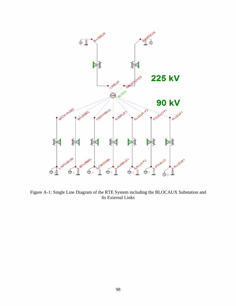
98
Figure A-1: Single Line Diagram of the RTE System including the BLOCAUX Substation and
Its External Links
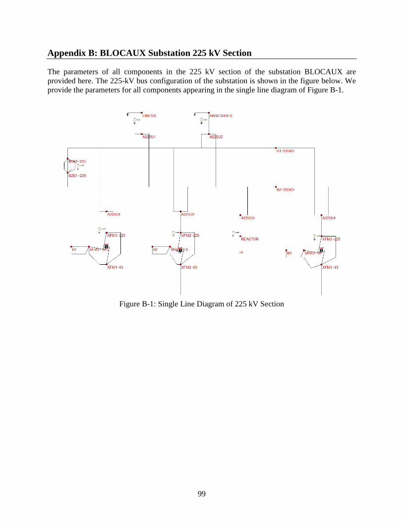
99
Appendix B: BLOCAUX Substation 225 kV Section
The parameters of all components in the 225 kV section of the substation BLOCAUX are provided here. The 225-kV bus configuration of the substation is shown in the figure below. We provide the parameters for all components appearing in the single line diagram of Figure B-1.
Figure B-1: Single Line Diagram of 225 kV Section

100
Figure B-2: 245 kV Shunt Reactor Parameters

101
Figure B-3: 225/93/10.5 kV Transformer 641 Parameters

102
Figure B-4: 225/93/9.9 kV Transformer 642 Parameters

103
Figure B-5: 225/93/10.0 kV Transformer 643 Parameters

104
Figure B-6: 2 Winding Transformer 1 Parameters

105
Figure B-7: 2 Winding Transformer 2 Parameters
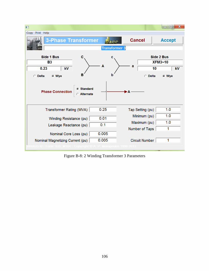
106
Figure B-8: 2 Winding Transformer 3 Parameters

107
Appendix C: BLOCAUX Substation 90 kV Section
The parameters of all components in the 90 kV section of the substation BLOCAUX are provided here. The 90-kV bus configuration of the substation is shown in Figure C-1. We provide the parameters for all components appearing in the single line diagram of Figure C-1.
Figure C-1: Single Line Diagram of 90 kV Section

108
Appendix D: Cables Between 225 kV and 90 kV Section
The parameters of the three cables connecting the 225 kV and 90 kV sections of the substation BLOCAUX are provided here. The three 90 kV cables connect the 90 kV section to the 90 kV side of the transformers in the 225 kV section.
Figure D-1: 90 kV cable 1 Parameters, Inside Substation

109
Figure D-2: 90 kV cable 2 Parameters, Inside Substation

110
Figure D-3: 90 kV cable 3 Parameters, Inside Substation

111
Appendix E: 225 kV External System
The parameters of all components in the external 225 kV system are provided here. The single line diagram is shown in Figure E-1.
Figure E-1: Single Line Diagram of the External 225 kV System
There are two voltage sources and two transmission lines connecting the sources to the substation BLOCAUX. The parameters of the voltage sources Limeux and Argeouves are given in the Figure E-2 and Figure E-3, respectively. The 225 kV transmission line parameters are given as in Figures E-4 and Figure E-5.

112
Figure E-2: 225 kV Source Limeux Parameters

113
Figure E-3: 225 kV Source Argeouves Parameters

114
Figure E-4: 225 kV Transmission Line From S-Limeux to Limeux Parameters The detailed data of this transmission line is not provided by Feb 05, 2017. It is modelled using the same tower structure as for line From Argeouves to BLOCAUX substation. Table below provides a comparison of the modeled line parameters with the provided data.
blocaux limeux WinIGS Model Rd 0.721 0.813 Xd 5.419 5.242 R0 4.68 4.126 X0 7.652 14.62

115
Figure E-5: 225 kV Trasmission Line From Argeouves to S-Argevs Parameters
Based on the provided data, it is seen that this line has different sections with and without the guard conductor. Also, the guard conductor is different and there are two types of those. Therefore, both guard conductor types are modelled as well as the phase conductors. Tower structure is also modified to with-guard and no-guard. Table below provides a comparison of the modeled line parameters with the provided data.
argoeuvre blocaux WinIGS Model
Rd 2.47 2.726 Xd 16.443 17.589 R0 8.79 10.841 X0 52.472 61.797

116
Appendix F: 90 kV External System
The parameters of all components in the external 90 kV system are provided here. The system is shown in Figure F-1.
Figure F-1: Single Line Diagram of the External 90 kV System
Because of lack of information, we applied a load at the other ends of the 90 kV lines. We expect that in the final model we will have an equivalent representation of the stem at the other end of the 90 kV circuits. The parameters of the external 90 kV transmission lines are given in Figures F-2 to F-8.

117
Figure F-2: 90 kV Transmission Line From Fouilloy1 to L-Fouillo Parameters
Table below provides a comparison of the modeled line parameters with the provided data.
Blocaux - Fouil 1 WinIGS Model Rd 0.79 0.809 Xd 2.11 1.954 R0 2.209 2.369 X0 6.639 5.908

118
Figure F-3: 90 kV Transmission Line From L-Croixra to Croixraul Parameters
Similar to the “argoeuvre blocaux” line, this line (“blocaux croiraux”) has also sections with and without guard conductor. Therefore, both cases are considered in the model. Table below provides a comparison of the modeled line parameters with the provided data.
blocaux croiraux WinIGS Model Rd 3.28 3.328 Xd 8.44 8.063 R0 7.153 7.282 X0 28.989 29.515
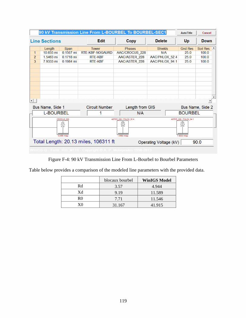
119
Figure F-4: 90 kV Transmission Line From L-Bourbel to Bourbel Parameters
Table below provides a comparison of the modeled line parameters with the provided data.
blocaux bourbel WinIGS Model Rd 3.57 4.944 Xd 9.19 11.589 R0 7.71 11.546 X0 31.167 41.915

120
Figure F-5: 90 kV Transmission Line From L-Aumale1 to Aumale1 Parameters
Table below provides a comparison of the modeled line parameters with the provided data.
aumal blocaux WinIGS Model Rd 0.32 0.369 Xd 0.83 0.906 R0 0.746 0.744 X0 2.778 3.355

121
Figure F-6: 90 kV Transmission Line From Alleux~F2 to L-Allx-F2 Parameters
Table below provides a comparison of the modeled line parameters with the provided data. The difference between the provided data and the modelled values might be due to the fact that the model considers all the line sections in parameter calculation from the “Blocaux” substation up to the load at the end of the line. However, as the line name shows: “ALLEUX (GRANDVILLIERS-BLOCAUX-FOUILLIOY 2”, it has a substation on the way. Thus, it is highly probable that the provided data is only for one of these sections since they are lower than the modeled values.
Blocaux - Fouil 2 WinIGS Model Rd 0.78 2.601 Xd 2.08 6.280 R0 1.867 6.283 X0 6.79 22.381

122
Figure F-7: 90 kV Transmission Line From Alleux1 to L-Alleux1 Parameters
Table below provides a comparison of the modeled line parameters with the provided data.
Alleux blocaux WinIGS Model Rd 2.518 2.522 Xd 6.702 6.072 R0 6.672 6.684 X0 21.033 20.689

123
Figure F-8: 90 kV Transmission Line From L-NFCHAUM to NFCH~AUM2 Parameters
Table below provides a comparison of the modeled line parameters with the provided data. Again, since the line has passed a substation on the way to the load, the provided data that is for only one of these sections differs from the the modeled values that are calculated for the line from “Blocaux” substation to the load.
aumal blocaux WinIGS Model Rd 0.31 4.024 Xd 0.82 12.392 R0 0.733 9.001 X0 2.685 46.476

124
Appendix G: Definition of Protection Zones Under Consideration
This Appendix defines four protection zones. These zones are targeted for application of the setting-less protective relay. It should be understood that these zones do not represent all the protection zones of this substation. Each protection zone is presented in terms of the following:
1. The physical system to be protected. The protection zone is connected to the rest of the system with interrupting devices (breakers).
2. The merging units or data acquisition system that perform measurements at the protection zone. The specific measurements are identified.

125
Protection Zone 1
This protection zone comprises the 90 kV Cable 1 plus the 225 kV/93 kV/10.5 kV Transformer 641. The protection zone can be isolated from the system by the breakers: the Breaker 1_1 and Breaker 1_2. Three merging units (Merging Unit 1, 2 and 8) collect measurements to be fed into the setting-less relay.
Figure G-1: Protection Zone 1

126
Figure G-2: 225 kV / 93 kV / 10.5 kV Transformer 641 Parameters

127
Figure G-3: 90 kV Cable 1 Parameters

128
Figure G-4: Merging Unit 1 (Captures the Measurements of 225 kV/93 kV /10.5 kV Transformer
641)

129
Figure G-5: Instrumentation Channels of Merging Unit 1
Figure G-6: Measurement Channels of Merging Unit 1

130
Figure G-7: Merging Unit 2 (Captures the Measurements of 90 kV Cable 1)

131
Figure G-8: Instrumentation Channels of Merging Unit 2
Figure G-9: Measurement Channels of Merging Unit 2

132
Figure G-10: Merging Unit 8 (Captures the Voltage Measurements of Bus B1B2~225 kV)

133
Figure G-11: Instrumentation Channels of Merging Unit 8
Figure G-12: Measurement Channels of Merging Unit 8

134
Protection Zone 2
This protection zone comprises the 90 kV Cable 2 plus the 225 kV/93 kV/9.9 kV Transformer 642. The protection zone can be isolated from the system by the breakers: the Breaker 2_1 and Breaker 2_2. Three merging units (Merging Unit 3, 4 and 8) collect measurements to be fed into the setting-less relay.
Figure G-13: Protection Zone 2

135
Figure G-14: 225 kV / 93 kV Transformer 642 Parameters

136
Figure G-15: 90 kV Cable 2 Parameters

137
Figure G-16: Merging Unit 3 (Captures the Measurements of 225 kV/93 kV Transformer 642)

138
Figure G-17: Instrumentation Channels of Merging Unit 3
Figure G-18: Measurement Channels of Merging Unit 3

139
Figure G-19: Merging Unit 4 (Captures the Measurements of 90 kV Cable 2)

140
Figure G-20: Instrumentation Channels of Merging Unit 4
Figure G-21: Measurement Channels of Merging Unit 4

141
Protection Zone 3
This protection zone comprises the 90 kV Cable 3 plus the 225 kV/93 kV/10.0 kV Transformer 643. The protection zone can be isolated from the system by the breakers: the Breaker 3_1 and Breaker 3_2. Three merging units (Merging Unit 5, 6 and 8) collect measurements to be fed into the setting-less relay.
Figure G-22: Protection Zone 3

142
Figure G-23: 225 kV / 93 kV Transformer 643 Parameters

143
Figure G-24: 90 kV Cable 3 Parameters

144
Figure G-25: Merging Unit 5 (Capture the Measurements of 225 kV/93 kV Transformer 643)

145
Figure G-26: Instrumentation Channels of Merging Unit 5
Figure G-27: Measurement Channels of Merging Unit 5

146
Figure G-28: Merging Unit 6 (Captures the Measurements of 90 kV Cable 3)

147
Figure G-29: Instrumentation Channels of Merging Unit 6
Figure G-30: Measurement Channels of Merging Unit 6

148
Protection Zone 4
This protection zone comprises the 245 kV Shunt Reactor. The protection zone can be isolated from the system by the breaker: the Breaker 4. Two merging unit (Merging Unit 7 and 8) collect measurements to be fed into the setting-less relay.
Figure G-31: Protection Zone 4

149
Figure G-32: 245 kV Shunt Reactor Parameters

150
Figure G-33: Merging Unit 7 (Captures the Measurements of 245 kV Shunt Reactor)

151
Figure G-34: Instrumentation Channels of Merging Unit 7
Figure G-35: Measurement Channels of Merging Unit 7

152
References
[1] A. P. Sakis Meliopoulos, Anjan Bose, PSERC Publication 10-17, Substation of the Future: A Feasibility Study, October 2010.
[2] A. P. Sakis Meliopoulos, G. Cokkinides, R. Huang, E. Farantatos, S. Choi, Y. Lee , “Wide Area Dynamic Monitoring and Stability Controls”, IREP Symposium 2010, Bulk Power System Dynamics and Control VIII, Buzios, Brazil, August 1-6, 2010.
[3] P. Sakis Meliopoulos, George Cokkinides, Renke Huang, Evangelos Farantatos, Sungyun Choi, Yonghee Lee and Xuebei Yu, "Smart Grid Technologies for Autonomous Operation and Control", IEEE Transactions on Smart Grid, Vol 2, No 1, March 2011.
[4] Sungyun Choi, Yonghee Lee, George Cokkinides and A. P. Sakis Meliopoulos, "Transformer Dynamic State Estimation Using Quadratic Integration", Proceedings of the 2011 Power Systems Conference & Exposition, Phoenix, AZ, March 20-23, 2011.
[5] Sungyun Choi, Yonghee Lee, George Cokkinides, and A. P. Meliopoulos, "Dynamically Adaptive Transformer Protection Using Dynamic State Estimation", Proceedings of the PAC World Conference 2011, Dublin, Ireland, June 27-30, 2011.
[6] A. P. Sakis Meliopoulos, George Cokkinides, Sungyun Choi, Evangelos Farantatos, Renke Huang and Yonghee Lee, "Symbolic Integration and Autonomous State Estimation: Building Blocks for an Intelligent Power Grid", Proceedings of the 2011 ISAP, Xersonissos, Crete, Greece, September 25-28, 2011.
[7] P. Meliopoulos, E. Polymeneas, Zhenyu Tan, Renke Huang, and Dongbo Zhao, “Advanced Distribution Management System”, IEEE Transsactions on Smart Grid.
[8] Sungyun Choi, Yonghee Lee, George Cokkinides, and A. P. Meliopoulos, "Dynamically Adaptive Transformer Protection Using Dynamic State Estimation", Proceedings of the PAC World Conference 2011, Dublin, Ireland, June 27-30, 2011.
[9] E. Farantatos, R. Huang, G. Cokkinides, A. P. Sakis Meliopoulos, B. Fardanesh, and G. Stefopoulos, "Advanced Disturbance Recording and Playback Enabled by a Distributed Dynamic State Estimation Including Bad Data Detection and Topology Change Identification", Proceedings of the IEEE-PES 2012 General Meeting, San Diego, CA, July 22-26, 2012.
[10] M. Kezunovic, V. Vittal, S. Meliopoulos, M. Venkatasubramanian and A. Sprintson, "Synchrophasors and the Smart Grid", Proceedings of the IEEE-PES 2012 General Meeting, San Diego, CA, July 22-26, 2012.
[11] A. P. Sakis Meliopoulos, "Update on the Substation Based Distributed State Estimator and Field Experience", Proceedings of the IEEE-PES 2012 General Meeting, San Diego, CA, July 22-26, 2012.
[12] A. P. Sakis Meliopoulos, George Cokkinides, Zhenyu Tan, Sungyun Choi, Yonghee Lee, and Paul Myrda, "Setting-less Protection: Feasibility Study", Proceedings of the of the 46st Annual Hawaii International Conference on System Sciences, Maui, HI, January 7-10, 2013.
[13] Sungyun Choi, A. P. Meliopoulos and Ratnesh Sharma, “Autonomous State Estimation Based Diagnostic System in Smart Grid”, Proceedings of the 2013 IEEE PES Innovative Smart Grid Technologies, Washington, DC, Feb 24-27, 2013.