Using Clustering Of Electricity ConsumersTo Produce More Accurate Predictions#1 R<-Slovakia meetup

Peter Laurinec22.3.2017

FIIT STU

R <- Slovakia

0

Why are we here? Rrrr

CRAN - about 10300 packages -https://cran.r-project.org/web/packages/.Popularity - http://redmonk.com/sogrady/:

1

Why prediction of electricity consumption?

Important for:

• Distribution (utility)companies. Producers ofelectricity. Overload.

• Deregularization of market

• Buy and sell of electricity.

• Source of energy - wind andphoto-voltaic power-plant.Hardly predictable.

• Active consumers. producer+ consumer⇒ prosumer.

• Optimal settings of bill.

2

Smart grid

• smart meter

• demand response

• smart cities

Good for:

• Sustainability - Blackouts...

• Green energy

• Saving energy

• Dynamic tariffs⇒ savingmoney

3

Slovak data

• Number of consumers are 21502. From that 11281 are OK. Enterprises.• Time interval of measurements: 01.07.2011 – 14.05.2015. But mainly fromthe 01.07.2013. 96 measurements per day.

Irish data:• Number of consumers are 6435. From that 3639 are residences.• Time interval: 14.7.2009 – 31.12.2010. 48 measurements per day. 4

Smart meter data

OOM_ID DIAGRAM_ID TIME LOAD TYPE_OF_OOM DATE ZIP

1: 11 202004 −45 4.598 O 01/01/2014 40132: 11 202004 195 4.087 O 01/01/2014 40133: 11 202004 −30 5.108 O 01/01/2014 40134: 11 202004 345 4.598 O 01/01/2014 40135: 11 202004 825 2.554 O 01/01/2014 40136: 11 202004 870 2.554 O 01/01/2014 4013

41312836: 20970 14922842 90 18.783 O 14/02/2015 401141312837: 20970 14922842 75 20.581 O 14/02/2015 401141312838: 20970 14922842 60 18.583 O 14/02/2015 401141312839: 20970 14922842 45 18.983 O 14/02/2015 401141312840: 20970 14922842 30 17.384 O 14/02/2015 401141312841: 20970 14922842 15 18.583 O 14/02/2015 4011 5

Random consumer from Kosice vol. 1

6

Random consumer from Kosice vol. 2

7

Aggregate load from Zilina

8

Random consumer from Ireland

9

Aggregate load from Ireland

10

R <- ”Forecasting”

10

STLF - Short Term Load Forecasting

• Prediction (forecast) for 1 day ahead (96 resp. 48measurements). Short term forecasting.

• Strong time dependence. Seasonalities (daily, weekly,yearly). Holidays. Weather.

• Accuracy of predictions (in %) - MAPE (Mean AbsolutePercentage Error).

MAPE = 100× 1n

n∑t=1

|xt − x̂t|xt

11

Methods for prediction of time series

Time series analysisARIMA, Holt-Winters exponential smoothing, decomposition TS...

Linear regressionMultiple linear regression, robust LR, GAM (Generalized AdditiveModel).

Machine learning

• Neural nets

• Support Vector Regression

• Regression trees and forests

Ensemble learningLinear combination of predictions.

12

Weekly profile

13

Time series analysis methods

ARIMA, exponential smoothing and co.

• Not best for multiple seasonal time series.

• Solution: Creation of separate models for different daysin week.

• Solution: Set higher period - 7 ∗ period. We need at least 3periods in training set.

• Solution: Double-seasonal Holt-Winters (dshw, tbats).

• Solution: SARIMA. ARIMAX - ARIMA plus extra predictors by FFT(auto.arima(ts, xreg)).

14

Fourier transform

fourier in forecastload_msts <- msts(load,

seasonal.periods = c(freq, freq * 7))fourier(load_msts, K = c(6, 6*2))

15

Time series analysis

• Solution: Decomposition of time series to three parts - seasonal, trend,remainder (noise).

• Many different methods. STL decomposition (seasonal decompositionof time series by loess).

• Moving Average (decompose). Exponential smoothing...

16

Decomposition - STL

stl, ggseas with period 48

17

Decomposition - STL vol.2

stl, ggseas with period 48 ∗ 7

18

Decomposition - EXP

tbats in forecast

19

Temporal Hierarchical Forecasting

thief - http://robjhyndman.com/hyndsight/thief/

20

Regression methods

• MLR (OLS), RLM 1 (M-estimate), SVR 2

• Dummy (binary) variables3

Load D1 D2 D3 D4 D5 D6 D7 D8 D9 … W1 W2 …

1: 0.402 1 0 0 0 0 0 0 0 0 1 02: 0.503 0 1 0 0 0 0 0 0 0 1 03: 0.338 0 0 1 0 0 0 0 0 0 1 04: 0.337 0 0 0 1 0 0 0 0 0 1 05: 0.340 0 0 0 0 1 0 0 0 0 1 06: 0.340 0 0 0 0 0 1 0 0 0 1 07: 0.340 0 0 0 0 0 0 1 0 0 1 08: 0.338 0 0 0 0 0 0 0 1 0 1 09: 0.339 0 0 0 0 0 0 0 0 1 1 0... . . . ...

...

1rlm - MASS2ksvm(..., eps, C) - kernlab3model.matrix(∼ 0 + as.factor(Day) + as.factor(Week))

21

Linear Regression

Interactions! MLR and GAM 4.

4https://petolau.github.io/22

Trees and Forests

• Dummy variables aren’t appropriate.• CART 5, Extremely Randomized Trees 6, Bagging 7.

Daily and Weekly seasonal vector:

Day = (1, 2, . . . , freq, 1, 2, . . . , freq, . . . )

Week = (1, 1, . . . , 1, 2, 2, . . . , 2, . . . , 7, 1, 1, . . . ),

where freq is a period (48 resp. 96).

5rpart6extraTrees7RWeka

23

rpart

rpart.plot::rpart.plot

24

Forests and ctree

• Ctree (party), Extreme Gradient Boosting (xgboost), RandomForest.

Daily and weekly seasonal vector in form of sine and cosine:

Day = (1, 2, . . . , freq, 1, 2, . . . , freq, . . . )

Week = (1, 1, . . . , 1, 2, 2, . . . , 2, . . . , 7, 1, 1, . . . )

sin(2π Dayfreq ) + 12 resp.

cos(2π Dayfreq ) + 12

sin(2πWeek7 ) + 12 resp.

cos(2πWeek7 ) + 12 ,

where freq is a period (48 resp. 96).

• lag, seasonal part from decomposition

25

Neural nets

• Feedforward, recurrent, multilayer perceptron (MLP), deep.

• Lagged load. Denoised (detrended) load.

• Model for different days - similar day approach.

• Sine and cosine

• Fourier

Figure 1: Day Figure 2: Week26

Ensemble learning

• We can’t determine which model is best. Overfitting.

• Wisdom of crowds - set of models. Model weighting⇒ linearcombination.

• Adaptation of weights of prediction methods based onprediction error - median weighting.

etj = median(| xt − x̂tj |)

wt+1j = wtjmedian(et)

etjTraining set – sliding window.

27

Ensemble learning

• Heterogeneous ensemble model.

• Improvement of 8− 12%.• Weighting of methods – optimization task.Genetic algorithm, PSO and others.

• Improvement of 5, 5%. Possible overfit.

28

Ensemble learning with clustering

ctree + rpart trained on different data sets (sampling withreplacement). ”Weak learners”.Pre-process - PCA→ K-means. + unsupervised.

29

R <- ”Cluster Analysis”

30

Creation of more predictable groups of consumers

Cluster Analysis! Unsupervised learning...

32

Cluster analysis in smart grids

Good for:

• Creation of consumer profiles, which can help byrecommendation to customers to save electricity.

• Detection of anomalies.• Neater monitoring of the smart grid (as a whole).• Emergency analysis.• Generation of more realistic synthetic data.• Last but not least, improve prediction methods toproduce more accurate predictions.

33

Cluster analysis in smart grids

Good for:

• Creation of consumer profiles, which can help byrecommendation to customers to save electricity.

• Detection of anomalies.• Neater monitoring of the smart grid (as a whole).• Emergency analysis.• Generation of more realistic synthetic data.• Last but not least, improve prediction methods toproduce more accurate predictions.

33

Cluster analysis in smart grids

Good for:

• Creation of consumer profiles, which can help byrecommendation to customers to save electricity.

• Detection of anomalies.

• Neater monitoring of the smart grid (as a whole).• Emergency analysis.• Generation of more realistic synthetic data.• Last but not least, improve prediction methods toproduce more accurate predictions.

33

Cluster analysis in smart grids

Good for:

• Creation of consumer profiles, which can help byrecommendation to customers to save electricity.

• Detection of anomalies.• Neater monitoring of the smart grid (as a whole).

• Emergency analysis.• Generation of more realistic synthetic data.• Last but not least, improve prediction methods toproduce more accurate predictions.

33

Cluster analysis in smart grids

Good for:

• Creation of consumer profiles, which can help byrecommendation to customers to save electricity.

• Detection of anomalies.• Neater monitoring of the smart grid (as a whole).• Emergency analysis.

• Generation of more realistic synthetic data.• Last but not least, improve prediction methods toproduce more accurate predictions.

33

Cluster analysis in smart grids

Good for:

• Creation of consumer profiles, which can help byrecommendation to customers to save electricity.

• Detection of anomalies.• Neater monitoring of the smart grid (as a whole).• Emergency analysis.• Generation of more realistic synthetic data.

• Last but not least, improve prediction methods toproduce more accurate predictions.

33

Cluster analysis in smart grids

Good for:

• Creation of consumer profiles, which can help byrecommendation to customers to save electricity.

• Detection of anomalies.• Neater monitoring of the smart grid (as a whole).• Emergency analysis.• Generation of more realistic synthetic data.• Last but not least, improve prediction methods toproduce more accurate predictions.

33

Approach

Aggregation with clustering

1. Set of time series of electricity consumption

2. Normalization (z-score)

3. Computation of representations of time series

4. Determination of optimal number of clusters K

5. Clustering of representations

6. Summation of K time series by found clusters

7. Training of K forecast models and the following forecast

8. Summation of forecasts and evaluation

34

Approach

Aggregation with clustering

1. Set of time series of electricity consumption

2. Normalization (z-score)

3. Computation of representations of time series

4. Determination of optimal number of clusters K

5. Clustering of representations

6. Summation of K time series by found clusters

7. Training of K forecast models and the following forecast

8. Summation of forecasts and evaluation

34

Approach

Aggregation with clustering

1. Set of time series of electricity consumption

2. Normalization (z-score)

3. Computation of representations of time series

4. Determination of optimal number of clusters K

5. Clustering of representations

6. Summation of K time series by found clusters

7. Training of K forecast models and the following forecast

8. Summation of forecasts and evaluation

34

Approach

Aggregation with clustering

1. Set of time series of electricity consumption

2. Normalization (z-score)

3. Computation of representations of time series

4. Determination of optimal number of clusters K

5. Clustering of representations

6. Summation of K time series by found clusters

7. Training of K forecast models and the following forecast

8. Summation of forecasts and evaluation

34

Approach

Aggregation with clustering

1. Set of time series of electricity consumption

2. Normalization (z-score)

3. Computation of representations of time series

4. Determination of optimal number of clusters K

5. Clustering of representations

6. Summation of K time series by found clusters

7. Training of K forecast models and the following forecast

8. Summation of forecasts and evaluation

34

Approach

Aggregation with clustering

1. Set of time series of electricity consumption

2. Normalization (z-score)

3. Computation of representations of time series

4. Determination of optimal number of clusters K

5. Clustering of representations

6. Summation of K time series by found clusters

7. Training of K forecast models and the following forecast

8. Summation of forecasts and evaluation

34

Approach

Aggregation with clustering

1. Set of time series of electricity consumption

2. Normalization (z-score)

3. Computation of representations of time series

4. Determination of optimal number of clusters K

5. Clustering of representations

6. Summation of K time series by found clusters

7. Training of K forecast models and the following forecast

8. Summation of forecasts and evaluation

34

Approach

Aggregation with clustering

1. Set of time series of electricity consumption

2. Normalization (z-score)

3. Computation of representations of time series

4. Determination of optimal number of clusters K

5. Clustering of representations

6. Summation of K time series by found clusters

7. Training of K forecast models and the following forecast

8. Summation of forecasts and evaluation

34

Approach

Aggregation with clustering

1. Set of time series of electricity consumption

2. Normalization (z-score)

3. Computation of representations of time series

4. Determination of optimal number of clusters K

5. Clustering of representations

6. Summation of K time series by found clusters

7. Training of K forecast models and the following forecast

8. Summation of forecasts and evaluation

34

Pre-processing

Normalization of time series - consumers.Best choice is to use z-score:

x− µ

σ

Alternative:x

max(x)

35

Representations of time series

36

Representations of time series

Why time series representations?

1. Reduce memory load.2. Accelerate subsequent machine learning algorithms.3. Implicitly remove noise from the data.4. Emphasize the essential characteristics of the data.

37

Methods of representations of time series

PAA - Piecewise Aggregate Approximation. Non data adaptive.n -> d. X̂ = (x̂1, . . . , x̂d).

x̂i =dn

(n/d)i∑j=(n/d)(i−1)+1

xj.

Not only average. Median, standard deviation, maximum...DWT, DFT...

38

Back to models - model based methods

• Representations based on statistical model.• Extraction of regression coefficients⇒ creation of dailyprofiles.

• Creation of representation which is long as frequency oftime series.

yi = β1xi1+β2xi2+ · · ·+βfreqxifreq+βweek1xiweek1+ · · ·+βweek7xiweek7+ εi,

where i = 1, . . . ,n

New representation: β̂ = (β̂1, . . . , β̂freq, β̂week1, . . . , β̂week7).Possible applicable methods:MLR, Robust Linear Model, L1-regression, Generalized AdditiveModel (GAM)...

39

Model based methods

• Triple Holt-Winters Exponential Smoothing.Last seasonal coefficients as representation.

1. Smoothing factors can be set automatically or manually.

• Mean and median daily profile.

40

Comparison

41

Comparison

42

Clipping - bit level representation

Data dictated.

x̂t ={

1 if xt > µ

0 otherwise

43

Clipping - RLE

RLE - Run Length Encoding. Sliding window - one day.

0 1 0 1 0 1 0 1 0 1 0 1 0 1 0 1 0 1 0 1 0 0 1 0 1 0 1 0 1 0 1 0 1 0 0 1 0 1 0 1 0 1 0 1 0 1 0 1 0 1 0

6 1 12 7 2 1 1 10 2 6 20 7 2 2 1 1 5 1 7 1 1 4 1 15 3 13 1 2 1 3 1 2 1 1 3 1 5 1 6 1 6 4 5 1 3 3 3 1 2 1 2

44

Clipping - final representation

1 7 1 10 6 7 2 1 1 1 1 3 1 1 1 1 1 1 1 4 1 3 1 1

6 12 2 1 2 20 2 1 5 7 0 4 15 13 2 3 2 1 3 5 6 6 5 3

Feature extraction: average, maximum, -average, -maximum …

45

Figure 3: Slovakia - factories Figure 4: Ireland - residential

Figure 5: Ireland - median daily profile

K-means

Euclidean distance. Centroids.

K-means++ - careful seeding of centroids.K-medoids, DBSCAN... 48

Finding optimal K

Manually or automatically set number of clusters. By internvalidity measure. Davies-Bouldin index...

1 2 3 4 5 6 7 8 9 10 11 12 13 14 15 16 17 18 19123 90 139 477 11 468 263 184 94 136 765 224 195 55 81 82 160 90 2

49

Results

Static data setOne clustering→ prediction with sliding window.Irish. GAM, RLM, PAA - 5.23% → okolo 4.22% MAPE.Slovak. Clip10, LM, DWT - 4.15% → okolo 3.97% MAPE.STL + EXP, STL + ARIMA, SVR, Bagging. Comparison of 17representations.

Batch processingBatch clustering→ prediction with sliding window (14 days).Irish. RLM, Median, GAM. Comparison of 10 prediction methods.Significant improvement in DSHW, STL + ARIMA, STL + ETS, SVR,RandomForest, Bagging and MLP.Best result: Bagging with GAM 3.68% against 3.82% MAPE.

55

R <- Tips and Tricks

55

Packages

List of all packages by name + short description.(https://cran.r-project.org/web/packages/available_packages_by_name.html)

56

Task Views

List of specific tasks (domains) - description of available packages andfunctions. (https://cran.r-project.org/web/views/)

57

Matrix Calculus

MRO 8. The Intel Math Kernel Library (MKL).

β̂ = (XTX)−1XTy8https://mran.microsoft.com/documents/rro/multithread/

58

Fast! SVD and PCA

Alternative to prcomp:

library(rARPACK)pc <- function(x, k) {# First center dataxc <- scale(x, center = TRUE, scale = TRUE)# Partial SVDdecomp <- svds(xc, k, nu = 0, nv = k)return(xc %*% decomp$v)

}

pc_mat <- pc(your_matrix, 2)

59

data.table

Nice syntax9:DT[i, j, by]

R i j bySQL where select or update group by

9https://github.com/Rdatatable/data.table/wiki/Getting-started

60

data.table

Advantages

• Memory efficient• Fast• Less code and functions

Reading large amount of .csv:files <- list.files(pattern = "*.csv")DT <- rbindlist(lapply(files, function(x)

cbind(fread(x), gsub(".csv", "", x))))

61

data.table

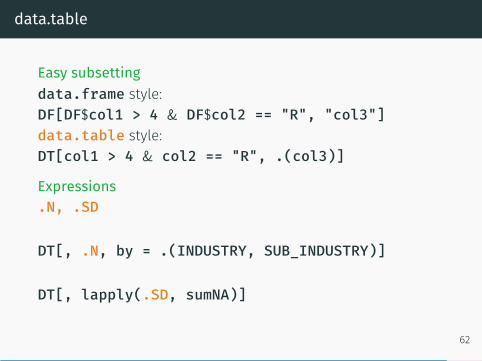
Easy subsettingdata.frame style:DF[DF$col1 > 4 & DF$col2 == "R", "col3"]data.table style:DT[col1 > 4 & col2 == "R", .(col3)]

Expressions.N, .SD

DT[, .N, by = .(INDUSTRY, SUB_INDUSTRY)]

DT[, lapply(.SD, sumNA)]

62

data.table

Changing DT by reference10

:=, set(), setkey(), setnames()

DF$R <- rep("love", Inf)DT[, R := rep("love", Inf)]

for(i in from:to)set(DT, row, column, new value)

10shallow vs deep copy

63

Vectorization and apply

library(parallel)

lmCoef <- function(X, Y) {beta <- solve(t(X) %*% X) %*% t(X) %*% as.vector(Y)as.vector(beta)

}

cl <- makeCluster(detectCores())clusterExport(cl, varlist = c("lmCoef", "modelMatrix",

"loadMatrix"), envir = environment())lm_mat <- parSapply(cl, 1:nrow(loadMatrix), function(i)

lmCoef(modelMatrix, as.vector(loadMatrix[i,])))stopCluster(cl)

64

Spark + R

sparklyr - Perform SQL queries through the sparklyr dplyrinterface. MLlib + extensions.

sparklyr http://spark.rstudio.com/index.htmlSparkR https://spark.apache.org/docs/2.0.1/sparkr.htmlComparison http://stackoverflow.com/questions/39494484/sparkr-vs-sparklyrHPC https://cran.r-project.org/web/views/HighPerformanceComputing.html 65

Graphics

ggplot2, googleVis, ggVis, dygraphs, plotly, animation, shiny...

66

Summary

• More accurate predictions are important.

• Clustering of electricity consumers have lot of applications.

• Prediction methods - different methods needs differentapproaches.

• Tips for more effective computing (programming) in R.

Blog: https://petolau.github.io/

Publications:https://www.researchgate.net/profile/Peter_Laurinec

Contact: laurinec.peter@gmail.com

67