RPL layer in Contiki with the Z1 Slide 1 Lower Layers PART...
23
Slide 1 Lower Layers PART 3: RPL layer in Contiki with the Z1 1 Remark: all numerical data refer to the parameters defined in IEEE802.15.4 for 32.5 Kbytes/s transmission in the 2.4 GHz frequency band. Kris Steenhaut - Jacques Tiberghien
Transcript of RPL layer in Contiki with the Z1 Slide 1 Lower Layers PART...
Slide 1
Lower Layers PART 3:
RPL layer in Contiki with the Z1
1
Remark: all numerical data refer to the parameters defined in IEEE802.15.4 for
32.5 Kbytes/s transmission in the 2.4 GHz frequency band.
Kris Steenhaut - Jacques Tiberghien

Slide 2
Routing in Wireless Sensor and Actuator Networks
2
• Almost all WSANs use multi-hop communication, thus requiring routing of messages through the network.
• Power grows at least as the square of the distance, but more often as the 4th power.
d d
P ~ (2d)2 = 4d2
P ~ d2 + d2 = 2d2

Slide 3
Routing in WSANs
Communication needs: 1. Collect : M2PFrom sensors to gatewayTo collect field data2. Distribute : P2MFrom gateway to sensorsTo download commands, parameters and software.3. Sensor to Sensor : P2PFrom one sensor to an otherTo run distributed data processing algorithms.
The Internet
Sensors
Radio links
Gateway(sink node)
The collect function is by far the most important, as most of the Wireless Sensor Networks are mainly intended for collecting data from the field. Power economy is often essential for extending lifetime and/or reducing maintenance costs. Latency can be an issue when the sensors can generate alarms. In most Wireless Sensor Networks the distribute protocol is only used for (exceptional) maintenance functions. Sensor to sensor communication is gaining importance because, as nodes become more powerful, local data pre-processing and data clustering can reduce the volume of data to send to the gateway. In Wireless Sensor and Actuator networks, the Distribute function is used to give commands to local actuators. Latency and reliability can be important issues. Some references: Philip Levis, Eric Brewer, David Culler, David Gay, Sam Madden, Neil Patel, Joe Polastre, Scott Shenker, Robert Szewczyk, Alec Woo: The Emergence of a Networking Primitive in Wireless Sensor Networks, Communications of the ACM, Volume 51, Number 7, July 2008.

Slide 4
Contiki Communication stacksConceptual view
M2P / P2MP2P
TCP/UDP
IP+RPL
6LOWPAN
MAC
RDC
Physical Layer
P2P + BROAD
M2P
COLLECT
Rime UIP6
Services
16 bit addresses 64 bit addresses
The Net subsystem of Contiki implements the communications facilities. This slide shows the simplified layered structure. Two different communication stacks are available: rime and UIP6. The rime stack offers simple, Contiki specific, communication facilities, including single-hop unicast (P2P) or broadcast (BROAD) and multi-hop multipoint to point (M2P) functionality. The UIP6 stack offers, multi-hop multipoint to point (M2P), point to multipoint (P2M) and point to point (P2P) functionality via the RPL routing protocol. By bypassing the transport and network layers, single hop unicast (P2P) and broadcast (BROAD) functionality is also available. The MAC, RDC and physical layers are common to both stacks, but their code contains many if(IPV6) and if(!IPV6) statements. The RPL routing protocol uses additional information about links gathered by the MAC and RDC layers. The most common example of this is the Estimated number of Transmissions needed to cross a specific link which is commonly used as a cost function for links.

Slide 5
IPv6 on Low Power and Lossy Networks?
5
Applications
TCP/UDP
MAC&PHY
IPv6
Applications
TCP/UDP
IEEE 802.15.4
RPL
6LowPan
A
GFE
I J K
B CD
H
L M
The Internet
The Low Power network is just one subnetThe sink node plays the role of a router
It is attractive to integrate low power and lossy networks in the internet, as it makes their access from anywhere and the development of applications much simpler. As these networks will often have a large number of nodes, only the IPv6 internet protocol has provisions for enough addresses. However, as low power networks have limitations, such as very limited memory capacity in the nodes, that other parts of the internet don’t have, their integration will need a specific architecture and specific protocols. The low power network will be considered as a specific subnet, connected to the internet through its sink node(s), which behave(s) like routers between the subnet and the internet. Reference : JeongGil Ko, Andreas Terzis, Stephen Dawson-Haggerty, David E. Culler, Jonathan W. Hui and Philip Levis: Connecting Low-Power and Lossy Networks to the Internet, IEEE Communications Magazine, April 2011, pp.96-101.

Slide 6
6LowPan – Why ?
6
TCP/UDP
IEEE 802.15.4
RPL
6LowPan
• Frame length : IPv6: <= 1280 bytes; IEEE 802.15.4: <= 81 bytes.Frame fragmentation & defragmentation
• Header length : IPv6 header >= 40 bytes; TCP header = 20 bytes, … No version field, no flow label, One subnet : 64 instead 128 bit addresses,Header compression
• Connectivity inside the subnet :• Single broadcast domain vs. multi-hop connectivityRoute-over architecture (see next slide)
001 resTLA SLANLA
3 13 8 24 18
INT
64
IPv6 address :
As specific protocols for low power and lossy networks using IPv6, there is first an adaptation layer between the network and the MAC layer. This layer is needed for several reasons: - first there is the length of the MAC frames: max 1280 bytes according to IPv6, while in
some configurations, IEEE 802.15.4 frames can be as short as 81 bytes. 6LowPan has to provide facilities to fragment and rebuild frames.
- Second, there is the size of the IPv6 headers. An IPv6 header, without extensions requires 40 bytes. If one adds a TCP header (20 bytes) to that, there are, in the shortest IEEE 802.15.4 frames just 21 bytes left for data. Fortunately, in the context of low power and lossy networks, lots of redundant or useless information can be removed from the headers. The version field is not needed as 6LowPan uses, by definition, v6. The flow label is also useless as no connection oriented, high-throughput data flows will be established in a low power and lossy network. As the entire low power network is considered as a single IPv6 subnet, the 64 most significant bits of the IPv6 addresses, which identify the subnet, are not needed for addressing inside the subnet.
- Third, an IPv6 subnet generally constitutes a single broadcast domain, while a low power and lossy network offers, most often, multi-hop connectivity, with the need for routing frames through the subnet. The RPL routing protocol has been proposed for this purpose and modified versions of the IPv6 Neighbor Discovery and configuration protocols can be used with RPL to integrate a low power and lossy network in an IPv6 internet.

Slide 7
Routing Protocol for Low Power and Lossy Networks
• RPL origin: “The Internet of things”.
– IETF working group for IPv6 routing.
– None of the existing protocols is adequate!
– New design combining interesting ideas of all.
• RPL Basic Mechanisms
– Routing based upon one or more Destination Oriented Directed Acyclic Graphs (DODAGs)
• Optimal routes between sink and all other nodes for both the collect and distribute data traffics.
• Redundant equivalent routes are kept for reliability in case of link or node failure.
– Multiple DODAGs if different optimisation criteria.
7
Some references: Internet Engineering Task Force (IETF), Request for Comments: 6550 - RPL: IPv6 Routing Protocol for Low-Power and Lossy Networks, ISSN: 2070-1721 , March 2012. Internet Engineering Task Force (IETF), Request for Comments: 6551 - Routing Metrics Used for Path Calculation in Low-Power and Lossy Networks, ISSN: 2070-1721, March 2012. Internet Engineering Task Force (IETF), Request for Comments: 6552 - Objective Function Zero for the Routing Protocol for Low-Power and Lossy Networks (RPL), 2070-1721, March 2012.

Slide 8
RPL: the DODAG
8
F
B
K
Flo
atin
g D
AG
J
A “floating DAG”
has no connection
with the sink. E.g :
failure of link A-B
A “grounded
DODAG” contains
the sink node and
offers routes from
all its nodes to
that sink node.
A
H
C
G
ED
I
NML
Grounded
DODAG
DODAG =
Destination
Oriented,
Directed,
Acyclic
Graph..
Routing in the RPL protocol is based upon the DODAG concept. It is a distributed data structure build-up and maintained during the WSAN usage. It is a kind of distributed routing table, build by the RPL algorithm and used for routing frames through the network. • DODAG = Destination Oriented Directed Acyclic Graph
Destination Oriented = All routes end in a Root Directed: one way edges Acyclic: no loops Nodes and links map into to those of the physical network
• Root = Node with no outgoing links • Roots interconnect the low power and lossy network with external networks such as
the Internet. DODAG roots correspond to the “sink” nodes traditionally used in the WSAN literature.

Slide 9
DODAG: neighbors and parents
9
The neighbors of a node are all the
nodes that can be reached via a single-
hop radio link.
The neighbors of G are C,D,H and L
A
H
C
G
ED
I
NML
Grounded
DODAG
The parents of a node are all
the neighbors that are on a
possible route from the node
to the sink.
Parents of G are C,D and H.
The preferred parent of a node is the
neighbor that is on the “best” route
from the node to the sink.
The preferred parent of G is H (will
be explained in a later slide).
To understand the building of a DODAG the concepts of neighbor, parent and preferred parent need to be introduced: - In a WSAN nodes communicate by radio. The neighbors of a node are all the nodes that
can communicate via single-hop radio links with that node. (To simplify this introduction, all radio links are supposed symmetric).
- A DODAG defines routes from all nodes to the root. The parents of a node are the neighbors of that node that belong to such a route. When a node has to send a message to the route, it suffices that it sends it to one of its parents.
- The quality of a route can be defined according to criteria dependent on the application (“Routing Metric”). A node should select among its parents the one that ensures the “best” route to the root, according to the selected criterion. This parent is the “preferred parent”.
- A node will always use its preferred parent to send messages to the route, unless the preferred parent is unavailable. In this case the node can use its other parents as back-up.

Slide 10
DODAG: the Routing Metric
10
1 2 -> 61
5 1
1
13
511 1
C1
D1
E4
G3
H2
I3
L4
M3
N3
A0
Each link and each node has an
associated cost, defined in terms of
the specific Routing Metric.
In this example nodes have no cost.
Each node computes the cost of the
best route to the root by adding to
the cost of the preferred parent the
cost to reach that preferred parent
3
Of course, no loops can be allowed
in the routing scheme. The situation
shown here could occur if suddenly
the cost of the link EA increases
For selecting the best route to the sink a “Routing Metric” is defined. This metric is similar to the “distance” parameters used in algorithms like Distance Vector. It gives the cost for reaching the sink from a specific node. The routing metric normally takes into account, depending on the application, not only the cost of traveling along a link, but also some node specific dynamic parameters such as the state of the battery. When a node has to select between several parents its preferred parent, that selection should minimize the routing metric. Of course, no loops may exist in the routes towards the root, because they would make the root unreachable from certain nodes.

Slide 11
DODAG: the RANK of nodes
11
1 21
5 11
511 1
C1/1
D1/1
E1/2
G3/3
H2/2
I2/3
L4/4
M3/3
N3/3
A0/0
3
1
All nodes have a rank, which is
some measure of the distance
between node and root. In this
example it is simply the hop-count.
To prevent the creation of routing
loops, all parents of a node must
have a rank lower than the rank of
that node. When a node joins the
DODAG, its rank is computed from
the data provided in the DIO
message. However a node is
authorized to increase its rank to
expand the set of its parents. In
this example G has increased its
rank from 2 to 3 in order to add H
to its parents.
To avoid creation of loops in the DODAG, the notion of “rank” has been introduced. In a DODAG, all nodes have a rank. This rank expresses in some way the distance from the node to the sink. This distance could be a simple hop-count or it could be a much more complex function, such as the average number of times a message needs to be retransmitted by radio to reach the root. The rank of a node is computed by an “Objective Function” (OF, not defined in the standard, because it should be specific for the application) , that takes into account the properties of the nodes and the links along the route between the node and the root. • The rank of a node should always be higher than the rank of its parents (this prevents
the creation of loops) • In older versions of the proposal nodes with the same rank were called “siblings”. • A node can voluntarily increase its rank in order to increase the set of its parents. • In these introductory slides, rank is considered equal to the hop count to the root.

Slide 12
RPL : Building the DODAG (1)
12
5 11
511 1
G3/3
H2/2
I2/3
L4/4
M3/3
N3/3
3
1
1 21
C1/
D1/
E1/
A0/0
The root initiates the building of a
new DODAG by sending DIO
messages to all its neighbors.
Nodes C,D and E join the DODAG.
and set their rank = 1.
Building a new DODAG is initiated by the root node of that DODAG. It assigns a unique DODAG identity to the new DODAG and sends DODAG Information Object (DIO) messages to all its neighbors. Each DIO messages carries the identity of the new DODAG, the rank of its sender (0 by definition for the root), the cost to reach the root from its sender (0 by definition for the root itself) as well as data about the link between its sender and its destination. The nodes receiving these DIO messages join the new DODAG. Their rank is, with the simple hop-count Objective Function used for this example, 1 as they are at one hop from the root.

Slide 13
RPL : Building the DODAG (2)
13
511 1
L M N
Nodes C,D and E have only one
parent, A. It is automatically their
preferred parent.
5 11
G H I
1 21
C1/1
D1/1
E1/2
A0/0
3
1
Nodes C,D and E set their cost
function
• The neighbors of the root have each one parent, the root, and their cost to the root is determined by the cost of the link from the root. Obviously the root is also their preferred parent.
Slide 14
RPL : Building the DODAG (3)
14
511 1
L M N
Node A ignores the DIO
messages because they
come from neighbors with a
higher rank.
Nodes G,H and I join the
DODAG. and set their rank.
1 21
5 11
C1/1
D1/1
E1/2
G2/
H2/
I2/
A0/0
3
1
Nodes C,D and E start sending DIO
messages to their neighbors
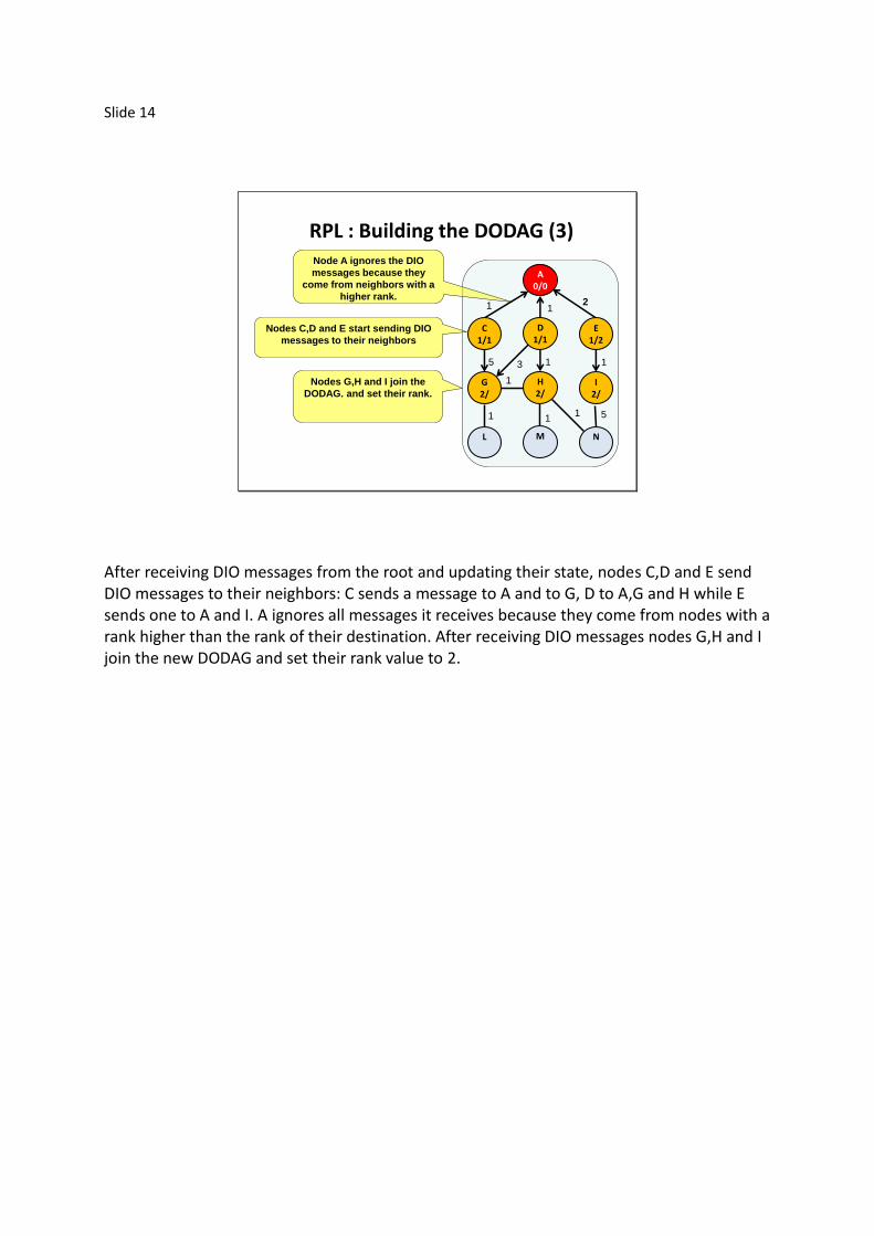
After receiving DIO messages from the root and updating their state, nodes C,D and E send DIO messages to their neighbors: C sends a message to A and to G, D to A,G and H while E sends one to A and I. A ignores all messages it receives because they come from nodes with a rank higher than the rank of their destination. After receiving DIO messages nodes G,H and I join the new DODAG and set their rank value to 2.

Slide 15
RPL : Building the DODAG (4)
15
511 1
L M N
Nodes G,H and L set up their list of
parents and select a preferred parent
5 11
G2/4
H2/2
I2/3
3
1Nodes G,H and L update their cost
figures
1 21
C1/1
D1/1
E1/2
A0/0
At this point the parents of G are C and D, with D as preferred parent. H and I each have only one parent, respectively D and E, wich become automatically preferred parents. G,H and I can now update their cost figures by adding to the cost of their preferred parent the cost of the link towards that preferred parent.

Slide 16
RPL : Building the DODAG (5)
16
511 1
L3/
M3/
N3/
Nodes C,D and ignore the
DIO messages from G,H
and I, because they come
from nodes with a higher
rank
5 11
G2/4
H2/2
I2/3
3
1
Nodes G,H and L send DIO
messages to all their neighbors
1 21
C1/1
D1/1
E1/2
A0/0
Nodes G,H and L join the
DODAG and set their rank
Nodes G,H and I now start sending DIO messages to their neighbors. G sends one to C,D,H and L. H sends one to D,G,M and N. I just sends one to E and N. C,D and E ignore the DIO messages they receive because the come from a node with a higher rank. L,M and N join the DODAG and set their rank to 3.

Slide 17
RPL : Building the DODAG (6)
17
511 1
L4/
M3/
N3/
5 11
G3/3
H2/2
I2/3
3
1
Nodes G discovers that using
neighbor H as a preferred parent
would result in a better cost figure,
but H has the same rank as G and
therefore can not be a parent of G.1 2
1
C1/1
D1/1
E1/2
A0/0
G now has to send DIO messages
to its neighbors, to inform them of
the change in rank.
Node G decides to increment its
rank to be allowed to adopt H as a
parent.
H can not become a parent of G, nor G a parent of H because G and H have the same rank but G discovers that the cost via H (3) is lower than the cost via its preferred parent D (4). Therefor G increments its rank by one unit. Now H can become a parent of G and it even beciomes its preferred parent. This change in its rank obliges G to send again DIO messages to its neighbors C,D,H and L. C,D and H ignore these messages because they come from a node with a higher rank. L will increment its own rank to 4.

Slide 18
RPL : Building the DODAG (7)
18
511 1
L4/4
M3/3
N3/3
5 11
G3/3
H2/2
I2/3
3
1
Now nodes L,M and N can select
their parents and their preferred
parent.
1 21
C1/1
D1/1
E1/2
A0/0
At this stage nodes L,M and N can set up their parents list and select their preferred parents. This completes the building of the DODAG as now all nodes are included.

Slide 19
RPL: Messages for routing
19
A
HF
C
G
EDB
I
NMLK
Grounded
DODAG
Flo
atin
g D
AG
J
DA
O
1 1 1
1 1 1
DIO
DIS
DIO (Destination Information Object) Transmitted downward by root and nodes in the DODAG for discovery, construction and maintenance.
DAO (Destination Advertisement Object) Propagates upwards destination information along the DODAG to populate the routing tables of ancestor nodes in support of the distribute traffic.
DIS (DODAG Information Solicitation) Discovers DODAGs in the neighborhood for grounding a floating DODAG. A DIS message is answered by a DIO

Slide 20
RPL: Collect, Distribute and P2P routing
20
A
H
C
G
ED
I
NML
1 1 1
1 1 1
A
H
C
G
ED
I
NML
1 1 1
1 1 1
A
H
C
G
ED
I
NML
1 1 1
1 1 1
Collect (M2P) Distribute (P2M) P2P
The collect protocol is used to collect data from all the nodes and to send it to the sink node (A). The routing simply consist in following the DODAG. The distribute protocol is just the opposite: data from the sink is sent to specific nodes. When connected to the DODAG, each node has sent to the sink a DAO message containing the name of its starting point. This message is augmented in each traversed node with the information necessary to retrace the itinerary in the opposite direction. These messages are kept in the sink and are used to establish the route of messages to be distributed. In the Peer to Peer mode, a message is first sent to the sink, and from there to its destination. If the nodes have enough memory to keep locally the information contained in the DOA messages, there is no need to go by the sink if the collect and distribute itineraries have common links.

Slide 21
RPL : Maintaining the DODAG
21
Basic mechanism:Each node sends DIO messages to its neighbors
When they receive DIO messages from their parentsWhen their local trickle timer expires
These DIO messages inform childrenAbout nodes leaving the DODAG (rank = ∞)About rank and/or cost changes
These DIO messages can cause DODAG repairs
The trickle timer is a timer with variable period.Whenever a change occurs the period decreasesIf no changes the period increases
DODAGs are maintained by means of DIO messages. These messages, issued by the root or by any node inform the children of each node of any changes that have occurred between that node and the root. This can be simple variations in the value of the cost function, it can be more important changes that cause a node to change its rank, possibly forcing other nodes to also change their rank (children need to have a rank higher than their parents). When a node wants to leave a DODAG (for instance when its battery gets low), it broadcasts an infinite rank, forcing all children to choose other parents. The trickle timers ensure that the DODAG structure is periodically checked by means of DIO messages. If links and nodes are stable the period of the trickle timers increases progressively up to a maximum value. When changes occur, that period returns to its minimum value, to ensure fast adaptations of the DODAG to new conditions.

Slide 22
The ETX cost function
22
ETX = Estimated number of transmissions from x to y.= Number of times a frame needs to be transmitted
over a link before being acknowledged.= (dxy x dyx)
-1 dxy = success rate from x to y.
Each node broadcasts precisely once per second a short message, each receiver counts during 10 seconds the number of broadcasts it receives from each neighbor.
dxy = (number of frames received from x by y) / 10
In the Contikimac RDC protocol, the number of times a frame is retransmitted is counted and averaged. This is used as ETX.
The ETX cost function has been introduced in 2003 and is considered a good cost function for multi-hop radio networks. It can easily be measured during network operation, it gives a realistic estimation of the amount of energy used for transmission. Reference: Douglas S. J. De Couto, Daniel Aguayo, John Bicket and Robert Morris: A High-Throughput Path Metric for Multi-Hop Wireless Routing, in the proceedings of MobiCom ’03, September 14–19, 2003, San Diego, California, USA.

Slide 23
Mac Layer optimization for RPL
23
511 1
L4/4
M3/3
N3/3
5 11
G3/3
H2/2
I2/3
3
1
1 21
C1/1
D1/1
E1/2
A0/0
Wake-up = t0 - δt
Wake-up = t0 - 2δt
Wake-up = t0 - 3δt
Wake-up = t0 – 4δtWake-up = t0 - 3δt
Synchronize receiver wake-ups to minimize latency along specific routes.
If mostly collect or distribute traffic exists, most messages follow a predictable path determined by a DODAG. This could be used to minimize message latency in a network using Radio Duty Cycling to optimize power usage. The DMAC protocol proposes to schedule the wake up periods of receivers along the paths taken by messages, so that on a multi-hop route, waiting times for receiver wake-ups should be minimized. The Contikimac protocol could be modified to schedule receiver wake-ups along DODAG routes to minimize wake up waiting. For collect traffic, the wake-up times should follow the ranks of the nodes. Reference: Gang Lu, Bhaskar Krishnamachari, Cauligi S. Raghavendra: An Adaptive Energy-Efficient andLow-Latency MAC for Data Gathering in Wireless Sensor Networks, Proceedings of the 18th International Parallel and Distributed Processing Symposium (IPDPS’04), 2004.