RPA: Design Tool for Liquid Rocket Engine...

RPA: Design Tool for Liquid Rocket Engine AnalysisAlexander Ponomarenko

[email protected]

http://www.lpre.de/resources/software/RPA_en.htm

January 2009

AbstractRPA (Rocket Propulsion Analysis) is a design tool for the performance prediction of the liquid-propellant rocket engines. RPA is written in Java and can be used under any operating system that has installed Java Runtime Environment (e.g. Mac OS ® X, Sun Solaris™, MS Windows™, any Linux etc). The tool can be used either as a standalone GUI application or as an object-oriented library.

This document presents the equations used for the combustion equilibrium and performance calculations. Results obtained from implementing these equations will be compared with results from equilibrium codes CEA2 and TDC.

1

mailto:[email protected]

http://www.lpre.de/resources/software/RPA_en.htm

ContentsSymbols.................................................................................................................................................3Analysis methods..................................................................................................................................4

Governing Equations for Combustion Equilibrium..........................................................................4Iteration Equations for Combustion Equilibrium.............................................................................7Iteration Procedure for Combustion Equilibrium.............................................................................8Thermodynamics Derivatives from Equilibrium Solution...............................................................8

Derivatives from Composition With Respect to Pressure............................................................8Derivatives from Composition With Respect to Temperature.....................................................9Derivatives from perfect gas state equation.................................................................................9Heat Capacity and Specific Heat.................................................................................................9Velocity of sound.......................................................................................................................11Density ......................................................................................................................................11Thermodynamic Derivatives for Frozen Flow...........................................................................11

Thermodynamic Data.....................................................................................................................12Theoretical Rocket Engine Performance........................................................................................12

Combustion Chamber Conditions..............................................................................................12Throat Conditions for Infinite-area combustion chamber.........................................................12Throat Conditions for Finite-area combustion chamber............................................................13Nozzle Exit Conditions..............................................................................................................15

Equilibrium Conditions.........................................................................................................15Frozen Conditions.................................................................................................................15

Theoretical Rocket Engine Performance...................................................................................16Computer Program RPA......................................................................................................................17

Graphical User Interface.................................................................................................................17Input Parameters........................................................................................................................17Output Data................................................................................................................................18

Verification.....................................................................................................................................19Conclusion...........................................................................................................................................22References...........................................................................................................................................23

2

SymbolsA area, m2 F area ratioNS total number of species, gaseous and condensedNG number of gaseous species

number of chemical elementsa ij stoichiometric coefficient, number of the atoms of element i per mole of the species

jn j moles of species j

N g moles of gaseous speciesR molar (universal) gas constant, R = 8.314472 J⋅K−1⋅mol−1 (ref. 9)H j

0 molar standard-state enthalpy for species j, J⋅mol−1

S j0 molar standard-state entropy for species j, J⋅K−1⋅mol−1

G j0 molar standard-state Gibbs energy for species j

p pressure, PaT temperature, Kw velocity, m/s density, kg/m3

V volume, m3

I s specific impulse, m/s

c∗ characteristic exhaust velocity, m/sC F thrust coefficient

Superscripts:

0 symbol for standard state symbol for molar parameter

symbol for dimensionless parameter

Subscripts:

inj injector face

c end of combustion chamber, or nozzle inlet section

t nozzle throat section

e nozzle exit section

0 symbol for assigned, initial or stagnation condition

3

Analysis methods

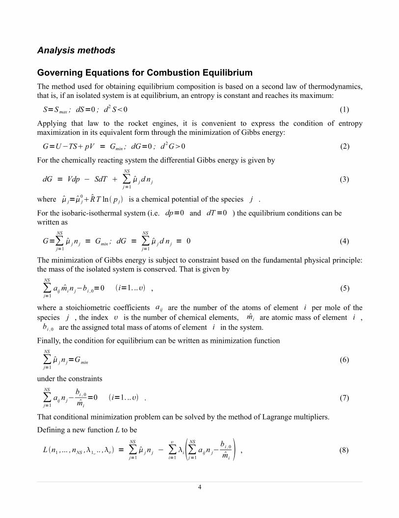
Governing Equations for Combustion EquilibriumThe method used for obtaining equilibrium composition is based on a second law of thermodynamics, that is, if an isolated system is at equilibrium, an entropy is constant and reaches its maximum:

S=S max ; dS=0 ; d2 S0 (1)

Applying that law to the rocket engines, it is convenient to express the condition of entropy maximization in its equivalent form through the minimization of Gibbs energy:

G=U−TS pV = Gmin ; dG=0 ; d 2G0 (2)

For the chemically reacting system the differential Gibbs energy is given by

dG = Vdp − SdT ∑j=1

NS

j d n j (3)

where j= j0 R T ln p j is a chemical potential of the species j .

For the isobaric-isothermal system (i.e. dp=0 and dT=0 ) the equilibrium conditions can be written as

G=∑j=1

NS

j n j = Gmin ; dG = ∑j=1

NS

j d n j = 0 (4)

The minimization of Gibbs energy is subject to constraint based on the fundamental physical principle: the mass of the isolated system is conserved. That is given by

∑j=1

NS

aij mi n j−b i ,0=0 i=1. .. , (5)

where a stoichiometric coefficients a ij are the number of the atoms of element i per mole of the species j , the index is the number of chemical elements, mi are atomic mass of element i ,

b i ,0 are the assigned total mass of atoms of element i in the system.

Finally, the condition for equilibrium can be written as minimization function

∑j=1

NS

j n j=Gmin (6)

under the constraints

∑j=1

NS

aij n j−bi , 0

mi=0 i=1. .. . (7)

That conditional minimization problem can be solved by the method of Lagrange multipliers.

Defining a new function L to be

L n1 ,... , nNS ,1,. .. , = ∑j=1

NS

j n j − ∑i=1

i∑j=1

NS

a ij n j−b i ,0

mi , (8)

4

where i are Lagrange multipliers, the condition for equilibrium becomes

j−∑i=1

i aij = 0 j=1... NS (9a)

∑j=1

NS

aij n j−bi , 0

mi= 0 i=1. .. (9b)

where

j={ j0 R T ln

n j

N g R T ln p

p0 j=1,... , NG

j0 j=NG1,... , NS } , j

0 =G j

0

n j= G j

0 , (10)

N g=∑j=1

NG

n j is the total mole number of gaseous species, and p0 is a standard-state pressure.

Reducing expressions and separating terms for gaseous and condensed phases, the final equations become

G j0 R T ln

n j

N g R T ln p

p0−∑

i=1

i a ij = 0 j=1... NG (11a)

G j0−∑

i=1

i a ij = 0 j=NG1. .. NS (11b)

∑j=1

NS

aij n j−bi , 0

mi= 0 i=1. .. (11c)

∑j=1

NG

n j−N g = 0 (11d)

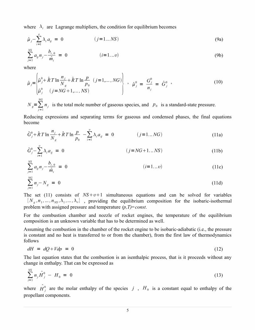
The set (11) consists of NS1 simultaneous equations and can be solved for variables{N g ,n1 , ... , nNS ,1 ,... ,} , providing the equilibrium composition for the isobaric-isothermal

problem with assigned pressure and temperature (p,T)=const. For the combustion chamber and nozzle of rocket engines, the temperature of the equilibrium composition is an unknown variable that has to be determined as well.

Assuming the combustion in the chamber of the rocket engine to be isobaric-adiabatic (i.e., the pressure is constant and no heat is transferred to or from the chamber), from the first law of thermodynamics follows

dH = dQVdp = 0 (12)

The last equation states that the combustion is an isenthalpic process, that is it proceeds without any change in enthalpy. That can be expressed as

∑j=1

NS

n jH j

0 − H 0 = 0 (13)

where H j0 are the molar enthalpy of the species j , H 0 is a constant equal to enthalpy of the

propellant components.

5

The final equations that permit the determination of equilibrium composition for thermodynamics state specified by an assigned pressure and enthalpy become

G j0 R T ln

n j

N g R T ln p

p0−∑

i=1

i aij = 0 j=1... NG (14a)

G j0−∑

i=1

i a ij = 0 j=NG1. .. NS (14b)

∑j=1

NS

aij n j−bi , 0

mi= 0 i=1. .. (14c)

∑j=1

NG

n j−N g = 0 (14d)

∑j=1

NS

n jH j

0 − H 0 = 0 (14e)

The set (14) consists of NS2 simultaneous equations and can be solved for variables{N g ,n1 , ... , nNS ,1 ,... , ,T } , providing the equilibrium composition for the isobaric-isenthalpic

problem with assigned pressure and enthalpy (p,H)=const.In order to determine the equilibrium composition for the nozzle flow, it is assumed that the entropy of the composition remains constant during expansion through the nozzle:

∑j=1

NS

n jS j − S 0 = 0 (15a)

S j={S j0− R ln

n j

N g− R ln p

p0 j=1,. .. , NG

S j0 j=NG1,... , NS } (15b)

where N g=∑j=1

NG

n j is the total mole number of gaseous species, p0 is a standard-state pressure, and

S0 is an entropy of the composition at the end of the combustion chamber.

Substituting last terms into the initial equations, and separating equations for gaseous and condensed phases, the final equations become

G j0 R T ln

n j

N g R T ln p

p0−∑

i=1

i a ij = 0 j=1... NG (16a)

G j0−∑

i=1

i a ij = 0 j=NG1. .. NS (16b)

∑j=1

NS

aij n j−bi , 0

mi= 0 i=1. .. (16c)

∑j=1

NG

n j−N g = 0 (16d)

6

∑j=1

NG

n j S j0− R ln

n j

N g− R ln p

p0 ∑

j=NG1

NS

n jS j

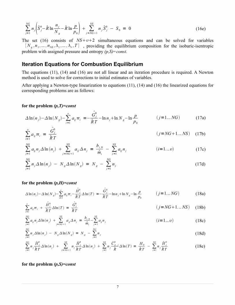
0 − S 0 = 0 (16e)

The set (16) consists of NS2 simultaneous equations and can be solved for variables{N g ,n1 , ... , nNS ,1 ,... , ,T } , providing the equilibrium composition for the isobaric-isentropic

problem with assigned pressure and entropy (p,S)=const.

Iteration Equations for Combustion EquilibriumThe equations (11), (14) and (16) are not all linear and an iteration procedure is required. A Newton method is used to solve for corrections to initial estimates of variables.

After applying a Newton-type linearization to equations (11), (14) and (16) the linearized equations for corresponding problems are as follows:

for the problem (p,T)=const

ln n j− ln N g−∑i=1

aij i =−G j

0

R T−ln n jln N g−ln p

p0

j=1... NG (17a)

∑i=1

a ij i =G j

0

R T j=NG1. .. NS (17b)

∑j=1

NG

aij n j ln n j ∑j=NG1

NS

a ij n j =b i ,0

mi− ∑

j=1

NS

aij n j i=1. .. (17c)

∑j=1

NG

n j ln n j − N g ln N g = N g − ∑j=1

NG

n j (17d)

for the problem (p,H)=const

ln n j − lnN g−∑i=1

aiji−H j

0

R T ln T =−

G j0

R T−lnn jln N g−ln p

p0

j=1... NG (18a)

∑i=1

aiji H j

0

R Tln T =

G j0

R T j=NG1. .. NS (18b)

∑j=1

NG


NS

a ijn j =bi , 0

mi−∑

j=1

NS

aij n j i=1... (18c)

∑j=1

NG

n jln n j − N g ln N g = N g − ∑j=1

NG

n j (18d)

∑j=1

NG

n j

H j0

R T ln n j ∑

j=NG1

NS

n j

H j0

R T ln n j ∑

j=1

NS

n j

C p , j0

R ln T =

H 0

R T− ∑

j=1

NS

n j

H j0

R T(18e)

for the problem (p,S)=const

7

ln n j − ln N g−∑i=1

aiji−H j

0

R T ln T =−

G j0

R T−ln n jln N g−ln p

p0

j=1... NG (19a)

∑i=1

aiji H j

0

R Tln T =

G j0

R T j=NG1. .. NS (19b)

∑j=1

NG


NS

a ijn j =bi , 0

mi−∑

j=1

NS

aij n j i=1. .. (19c)

∑j=1

NG

n jln n j − N g ln N g = N g − ∑j=1

NG

n j (19d)

∑j=1

NG [ S j0

R− lnn j−ln N g ln p

p01]n jln n j ∑

j=NG1

NS

n j

S j0

Rln n j ∑

j=1

NS

n j

C p , j0

R lnT

∑j=1

NG

n j ln N g =S 0

R− ∑

j=1

NG [ S j0

R− ln n j−ln N gln p

p0 ]n j − ∑j=NG1

NS

n j

S j0

R

(19e)

The set (17) consists of NS1 linear simultaneous equations and can be solved for correction variables { ln N g , ln n1 , ... , ln nNG , nNG1 ,... ,nNS ,1, ... ,} . The sets (18) and (19) each consist of NS2 linear simultaneous equations and can be solved for correction variables{ ln N g , ln n1 , ... , ln nNG ,n NG1 , ... ,nNS ,1, ... , , lnT } . Here a new variable i

defined as i=i

R T.

Iteration Procedure for Combustion EquilibriumThe solutions proceeds by solving the appropriate set of linear simultaneous equations and incrementally updating the number of moles for each species n j , the total moles N g and the temperature T (for the (p,H) and (p,S) problems) until the correction variables are within a specified tolerance. At each iteration, the updated set of linear equations is solved using a Lower-Upper (LU) matrix decomposition algorithm.

An initial estimates and controlling the divergence are made, as suggested by Gordon and McBride (ref. 3).

Thermodynamics Derivatives from Equilibrium Solution

Derivatives from Composition With Respect to PressureDifferentiating equations (11) with respect to pressure gives

∑i=1

a ij i

ln p T ln N g

ln p T− ln n j

ln p T = 1 j=1,... , NG (20a)

∑i=1

a ij i

ln p T = 0 j=NG1,. .. , NS (20b)

8

∑j=1

NG

akj n j ln n j

ln p T ∑j=NG1

NS

akj n j

ln p T = 0 k=1,. .. , (20c)

∑j=1

NG

n j ln n j

ln p T− N g ln N g

ln p T= 0 (20d)

The set (20) consists of NS1 linear simultaneous equations and can be solved for unknown

terms ln n1

ln p T , ... , ln nNS

ln p T

, ln N g

ln p T

, 1

ln p T ,... ,

ln p T .

Derivatives from Composition With Respect to TemperatureDifferentiating equations (11) with respect to temperature gives

∑j=1

NG

aij n j ln n j

ln T p ∑

j=NG1

NS

a ij n j

ln T p= 0 i=1,... , (21a)

∑i=1

aij i

ln T p= −

H j0

R T j=NG1,. .. , NS (21b)

∑j=1

NG

aij n j ln n j

ln T p ∑

j=NG1

NS

a ij n j

ln T p= 0 i=1,... , (21c)

∑j=1

NG

n j ln n j

ln T p− N g ln N g

ln T p= 0 (21d)

The set (21) consists of NS1 linear simultaneous equations and can be solved for unknown

terms ln n1

lnT p

, ... , ln nNS

ln T p

, ln N g

ln T p

, 1

lnT p, ... ,

ln T p.

Derivatives from perfect gas state equation

Differentiating equation of state pV =N gR T with respect to temperature gives

ln V ln T p

= ln N g

ln T p1 (22)

Differentiating equation of state with respect to temperature gives

ln V ln p T = ln N g

ln p T−1 (23)

Heat Capacity and Specific HeatHeat capacity of the thermodynamic system at constant pressure is defined as

9

C p = HT p

= [∑j=1

NS

n jH j

0]T

p

(24)

and after differentiation gives

C p = ∑j=1

NG

n j

H j0

T ln n j

ln T p ∑

j=NG1

NS H j0

T n j

ln T p ∑

j=1

NS

n jC p , j

0 (25)

Molar heat capacity and specific heat are

C p =C p

∑j=1

NS

n j(26)

and

c p =C p

m=

C p

m∑j=1

NS

n j

=C p

m (27)

correspondingly.

Relation between heat capacities can be expressed as

C p−C v = −TVT

p

2

V p T

= −T

V 2

T 2 ln V ln T p

2

Vp ln V

ln p T= − pV

T ln V lnT

p

2

lnV ln p T

= −N gR ln V ln T p

2

ln V ln p T

(28)

After substitution (22) and (23) into equation (28), the heat capacity of the thermodynamic system at constant volume can be found from the previous equation:

C v = C p N gR ln V lnT

p

2

ln V ln p T

(29)

Molar heat capacity and specific heat are

C v =C v

∑j=1

NS

n j(30)

and

cv =C v

m=

C v

m∑j=1

NS

n j

=C v

m (31)

correspondingly.

10

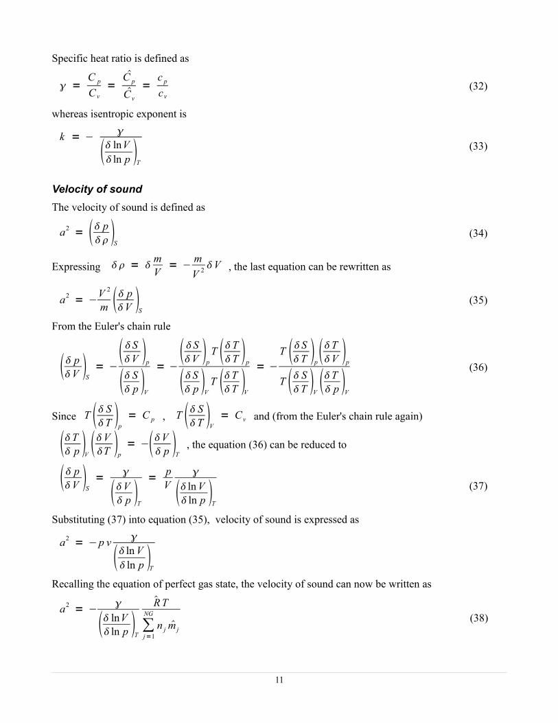
Specific heat ratio is defined as

=C p

C v=

C p

C v

=c p

cv (32)

whereas isentropic exponent is

k = −

lnV ln p T (33)

Velocity of soundThe velocity of sound is defined as

a2 = p S (34)

Expressing = mV

= − mV 2 V , the last equation can be rewritten as

a2 = −V 2

m pV

S(35)

From the Euler's chain rule

pV

S= −

SV

p

S p V

= −SV

pT T

T p

S p V T T

T V= −

T ST p

TV

p

T ST V T

p V(36)

Since T ST p

= C p , T ST V = C v and (from the Euler's chain rule again)

T p V V

T p= −V

p T , the equation (36) can be reduced to

pV

S=

V p T

= pV

ln V ln p T (37)

Substituting (37) into equation (35), velocity of sound is expressed as

a2 = −p v

ln V ln p T

Recalling the equation of perfect gas state, the velocity of sound can now be written as

a2 = −

lnV ln p T

R T

∑j=1

NG

n j m j(38)

11

Density

= p1000 N g

R T∑j=1

NS

n j m j

Thermodynamic Derivatives for Frozen FlowIt can be shown, that for the “frozen” flow where composition remains fixed, the mentioned derivatives can be reduced to

C p , f = ∑j=1

NS

n jC p , j

0 , (39)

C v , f = C p , f ∑j=1

NS

n jR , (40)

k f = f =C p , f

C v , f=

C p , f

C v , f

=c p , f

cv , f(41)

a f2 = k f

Rm

T (42)

Thermodynamic DataThe program supports the thermodynamic database in ASCII format (ref. 6) and can utilize original NASA database of McBride (ref. 4) as well as its enlargements (e.g. provided by Burcat and Ruscic, ref. 7). Both databases are included with the current program distribution.

For each reaction species the thermodynamic functions heat capacity, enthalpy and entropy as functions of temperature are given in the polynomial form using 9 constants as follows:

C p0

R= a1T−2 a2 T−1 a3 a4 T a5 T 2 a6T 3 a7T 4 (43)

H 0

RT= −a1T−2 a2ln T T−1 a3

a4

2T

a5

3T 2

a6

4T 3

a7

5T 4 a8T−1 (44)

S 0

R= −

a1

2T−2 − a2T−1 a3ln T a4 T

a5

2T 2

a6

3T 3

a7

4T 4 a9 (45)

Theoretical Rocket Engine PerformanceThe following assumptions are made for the calculation of the theoretic rocket performance: adiabatic, isenthalpic combustion; adiabatic, isentropic (frictionless and no dissipative losses) quasi-one-dimensional nozzle flow; ideal gas law; no dissipative losses.

Combustion Chamber ConditionsThe analysis is started by obtaining the combustion chamber equilibrium composition assuming the isobaric-isenthalpic combustion, followed by calculation of the thermodynamics derivatives from the equilibrium solution. The results include the number of moles for each species, combustion

12

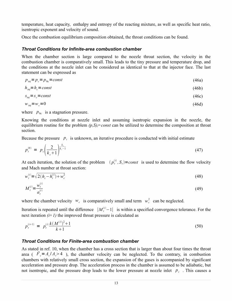
temperature, heat capacity, enthalpy and entropy of the reacting mixture, as well as specific heat ratio, isentropic exponent and velocity of sound.

Once the combustion equilibrium composition obtained, the throat conditions can be found.

Throat Conditions for Infinite-area combustion chamberWhen the chamber section is large compared to the nozzle throat section, the velocity in the combustion chamber is comparatively small. This leads to the tiny pressure and temperature drop, and the conditions at the nozzle inlet can be considered as identical to that at the injector face. The last statement can be expressed as

p inj=pc=p0c=const (46a)

h inj=hc=const (46b)

sinj=sc=const (46c)

w inj=w c=0 (46d)

where p0c is a stagnation pressure.

Knowing the conditions at nozzle inlet and assuming isentropic expansion in the nozzle, the equilibrium routine for the problem (p,S)t=const can be utilized to determine the composition at throat section.

Because the pressure p t is unknown, an iterative procedure is conducted with initial estimate

p t0 = pc 2

k c1 k c

k c−1 (47)

At each iteration, the solution of the problem p t i , S t =const is used to determine the flow velocity

and Mach number at throat section:

w ti =2hc−ht

i wc2 (48)

M ti =

wti

a ti (49)

where the chamber velocity w c is comparatively small and term w c2 can be neglected.

Iteration is repeated until the difference ∣M ti −1∣ is within a specified convergence tolerance. For the

next iteration (i+1) the improved throat pressure is calculated as

p ti1 = pt

i k M i21k1

(50)

Throat Conditions for Finite-area combustion chamberAs stated in ref. 10, when the chamber has a cross section that is larger than about four times the throat area ( F c=Ac /A t4 ), the chamber velocity can be neglected. To the contrary, in combustion chambers with relatively small cross section, the expansion of the gases is accompanied by significant acceleration and pressure drop. The acceleration process in the chamber is assumed to be adiabatic, but not isentropic, and the pressure drop leads to the lower pressure at nozzle inlet pc . This causes a

13

small loss in specific impulse.

Because both nozzle inlet pressure pc and nozzle throat pressure p t are unknown, two-level iterative procedure is conducted with initial estimates

pc0 = 1

c [1 k inj M c2

T pinj ] (51a)

where c is a characteristic Mach number at nozzle inlet obtained for subsonic flow from equation

1F c=k1

2 1

k−1c1− k−1k1

c2

1k−1 with assumption k=k inj ; M c is a Mach number that

corresponds to the calculated characteristic Mach number;

T=− lnV ln p T

pand c=1− k−1

k1c

2k

k−1 also with assumption k=k inj ;

c0= inj (51b)

For the assigned chamber contraction area ratio F c=Ac /At , the iteration proceeds as follows:

1. Assuming that velocity at injector face can be neglected, the velocity at the nozzle inlet is obtained from the momentum equation for steady one-dimensional flow:

wci = p inj−pc

i

ci (52)

2. If acceleration process in the chamber is adiabatic, the total enthalpy per unit mass is constant. Recalling that velocity at injector face can be neglected, the specific enthalpy at nozzle inlet can be expressed as

hc i=hinj−

w c i2

2(53)

3. Solution of the problem (p,H)c=const for the nozzle inlet section provides the entropy at nozzle inletSci .

4. Known conditions at nozzle inlet and assumption about an isentropic expansion in the nozzle allow to obtain the throat conditions (including throat pressure p t

i and density ti ), utilizing the

procedure similar to that for the infinite-area combustion chamber (equations 47 to 50).

5. From the continuity equation for steady quasi-one-dimensional flow, find the velocity at the nozzle inlet for the specified chamber contraction ratio:

wc=t w t

c i

1Fc

(54)

6. From the momentum equation, find the pressure at injector face that corresponds to the calculated pressure and velocity at the nozzle inlet:

p inj=pci c

i w c2 (55)

14

Iteration is repeated until the relative deviation∣p inj−p inj∣

pinjis within a specified convergence

tolerance. The improved nozzle inlet pressure for the next iteration (i+1) is calculated as

pci1=pc

i pinj

pinj(56)

The stagnation pressure at nozzle inlet section can be computed from

p0c= pc[1k c−1w c

2c

2k c pc ]k c

kc−1 (57)

Nozzle Exit Conditions

Equilibrium ConditionsEquilibrium conditions at section specified by assigned pressure pe

Knowing the conditions at nozzle throat and assuming isentropic expansion in the nozzle, the equilibrium routine for the problem (p,S)e=const can be directly utilized to determine the composition at nozzle exit section.

The corresponding nozzle area ratio can be obtained from

F e=t a t

e we(58)

Equilibrium conditions at section specified by assigned nozzle area ratio F e=Ae /A t

Knowing the conditions at nozzle throat and assuming isentropic expansion in the nozzle, the equilibrium routine for the problem (p,S)e=const can be utilized to determine the composition at nozzle exit section.

Because the pressure pe is unknown, an iterative procedure is conducted with initial estimate

pe0 =pc1− k−1

k1e

2k

k−1 with assumption k=k t (59)

where e is a characteristic Mach number at nozzle exit obtained for supersonic flow from equation

1F e=k1

2 1

k−1e1− k−1k1

e2

1k−1 also with assumption k=k t .

At each iteration, the solution of the problem p i , S e=const is used to determine the nozzle area ratio that corresponds to the assumed nozzle exit pressure:

wei =2 hc−h t

i wc2 (60)

F e i=

t at

e i we

i (61)

15

Iteration is repeated until the relative deviation∣ F e−F e

i∣F e

is within a specified convergence

tolerance. The improved nozzle exit pressure for the next iteration (i+1) is calculated as

pei1=pe

i F e i

Fe 2

(62)

Frozen ConditionsFor the frozen conditions it is assumed that chemical equilibrium is established within the nozzle section r between nozzle throat and nozzle exit. Once the reaction products passed through that section, the composition is considered to be invariant (frozen), and does not change.

That is, the nozzle exit composition is defined as {N g ,n1 , ... , nNS }e={N g , n1 , ... , nNS }r=const .

The remainder procedure is as follows.

Frozen conditions at section specified by assigned pressure pe

In that case the unknown variable T e can be determined from equation

∑j=1

NS

n jS je − S r = 0 (63a)

where S j={S j0− R ln

n j

N g− R ln p

p0 j=1,. .. , NG

S j0 j=NG1,... , NS } (63b)

Frozen conditions at section specified by assigned nozzle area ratio F e=Ae /A t

In that case the unknown variables {T e , pe} can be found from the following equations:

∑j=1

NS

n jS je − S r = 0 (64a)

where S j={S j0− R ln

n j

N g− R ln p

p0 j=1,. .. , NG

S j0 j=NG1,... , NS }

pg∑j=1

NG

n j m j = N gR T (64b)

F r =wtwr

(64c)

h w2

2 e= h

w 2

2 r

(64d)

The set of simultaneous equations (64a) to (64d) can be solved for variables {p , T , , w}e .

16

Theoretical Rocket Engine PerformanceThe following equations for the theoretical rocket engine performance obtained from ref. 10 and 11.

Characteristic exhaust velocity:

c∗=p0c

at t(65)

Specific impulse in a vacuum:

I svac=we

pe

we e(66)

Specific impulse at ambient pressure pH :

I sH=we

pe−pH

we e(67)

Optimum specific impulse ( pe=pH ):

I sopt=we (68)

Thrust coefficient in vacuum:

C Fvac=

I svac

c∗(69)

Optimum thrust coefficient:

C Fopt=

I sopt

c∗(70)

Note that the equation (67) can be used for nozzle conditions without flow separation caused by over-expansion. In order to correctly predict the nozzle performance under highly over-expanded conditions, a more accurate model that considers flow separation and shock waves is required.

Computer Program RPA

Graphical User Interface

Input ParametersThe minimal set of input parameters include

– combustion chamber pressure (expressed in Pascal, atm, bar or psia)

– propellant combination

– mixture ratio "O/F" or relative abundance of oxidizer (α) or mass fractions of each component;

– list of components at standard conditions or at assigned temperature (K);

– assigned enthalpy (kJ/kg or J/mol, optional).

When the minimal set of parameters is defined, the program calculates combustion equilibrium and

17

determines the properties of the reaction products.

Additional set of input parameters include nozzle analysis options:

– nozzle exit conditions

assigned nozzle exit pressure (Pascal, atm, bar od psia) or nozzle exit area ratio;

– nozzle inlet conditions (optional)

assigned chamber contraction area ratio or mass flow rate per unit combustion chamber area ( kg /m2⋅s );

– frozen flow (optional)

freezing at the assigned pressure (Pascal, atm, bar or psia) or at the assigned nozzle area ratio.

The complete set of input parameters can be stored in and loaded from the file system.

The program supports the following optional command-line switches:

language=en|de|ru to select the language of the user interface

country=US|DE|RU to select the country that affects the data output format

useEn=yes|no to allow the usage of thermodynamic database enlargement (provided by Burcat and Ruscic)

useEx=<path> to specify the external thermodynamic database

Output DataFor the minimal set of input parameters, results of thermodynamic calculations include combustion parameters and composition.

18

Illustration 1. Input parameters GUI

For the set of input parameters that includes nozzle analysis options, conditions at nozzle throat and nozzle exit, as well as theoretical rocket engine performance, will be determined.

VerificationThe tool was compared with a code CEA2 (Chemical Equilibrium and Applications 2) developed by Gordon and McBride (ref. 4) at NASA Glenn/Lewis Research Center, and TDC (ThermoDynamic Сalculation for LRE) developed at Moscow Aviation Institute (ref. 12).

To verify the RPA model and implementation, six test cases were selected (see Table 1).

Table 1. Test casesTest case 1 Test case 2 Test case 3 Test case 4 Test case 5 Test case 6

Oxidizer/Temperature, K LOX / 90.17 LOX / 90.17 LOX / 90.17 LOX / 90.17 LOX / 90.17 LOX / 90.17

Fuel/Temperature, K LH / 20.27 LH / 20.27 CH4 (L) / 111.643 CH4 (L) / 111.643 RP-1 / 298.15RG-1 / 293

RP-1 / 298.15

O/F ratio 5.5 5.5 3.2 3.2 2.6 2.6

Chamber pressure, MPa 10 10 10 10 10 10

Chamber contraction area ratio – 2 – 2 – 2

Nozzle exit area ratio 70 70 70 70 70 70

For all test cases, RPA and CEA2 were executed with identical input parameters.

Due to the fact that TDC does not support the calculation of rocket performance with finite area combustion chamber, RPA and TDC were compared for test cases 1, 3 and 5. Input parameters for both programs were identical excepting the test case 5: because of the differences in the used thermodynamic databases, RPA calculated the combustion of the fuel RP-1 at initial temperature 298.15 K whereas TDC calculated the combustion of the fuel RG-1 at initial temperature 293 K.

Tables 2 to 10 provide the results of thermodynamic calculations.

Perfect agreement was obtained between RPA and CEA2 codes.

19

Illustration 2. Output data GUI

Very good agreement with small deviations was obtained between RPA and TDC codes.

Table 2. Results of thermodynamics calculations for Test case 1RPA CEA2 TDC

Chamber temperature, K 3432.01 3432.01 3436.10

Characteristic velocity, m/s 2345.30 2345.30 2346.35

Thrust coefficient 1.87 (opt) 1.94 (vac)

1.8728 (opt)–

–1.93950 (vac)

Specific impulse, vac, m/s 4549.28 4549.20 4550.86

Specific impulse, opt, m/s 4392.36 4392.30 4393.77

Nozzle exit Mach number 4.69 4.69 4.67

Table 3. Results of thermodynamics calculations for Test case 2RPA CEA2

Chamber temperature, K 3432.01 3432.01

Nozzle inlet pressure, MPa 8.98100 8.98130

Characteristic velocity, m/s 2344.62 2344.60

Thrust coefficient (opt) 1.870 1.873

Specific impulse, vac, m/s 4548.97 4548.90

Specific impulse, opt, m/s 4391.94 4391.90

Nozzle exit Mach number 4.69 4.69

Table 4. Mole fractions in combustion chamber for Test cases 1 and 2Species RPA CEA2 TDC

H 0.02775 0.02775 0.02800

H2 0.30152 0.30152 0.30089

H2O 0.64016 0.64016 0.64195

H2O2 0.00001 0.00001 0.0

HO2 0.00001 0.00001 0.0

O 0.00140 0.00140 0.00143

O2 0.00115 0.00115 0.00116

OH 0.02799 0.02800 0.02658





1.9083 (opt)–

–1.9888 (vac)




20








Nozzle exit Mach number 4.43 4.43


CO 0.19733 0.19733 0.19811

CO2 0.11704 0.11704 0.11604

COOH 0.00002 0.00002 0.0

H 0.02155 0.02155 0.02224

H2 0.09898 0.09898 0.09868

H2O 0.49169 0.49169 0.49185

H2O2 0.00002 0.00002 0.0

HCO 0.00002 0.00002 0.0

HO2 0.00009 0.00009 0.0

O 0.00641 0.00641 0.00685

O2 0.01221 0.01221 0.01294

OH 0.05463 0.05463 0.05334





1.9152 (opt)–

–1.9888 (vac)








21

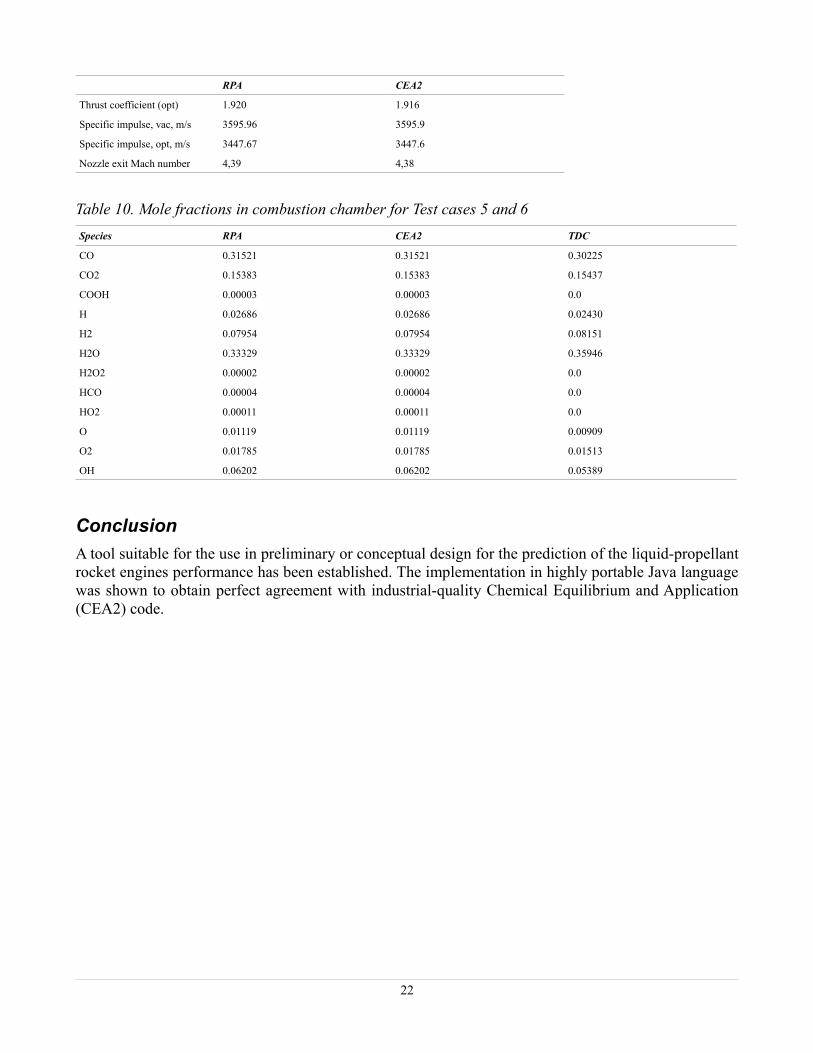
RPA CEA2




Nozzle exit Mach number 4,39 4,38


CO 0.31521 0.31521 0.30225

CO2 0.15383 0.15383 0.15437

COOH 0.00003 0.00003 0.0

H 0.02686 0.02686 0.02430

H2 0.07954 0.07954 0.08151

H2O 0.33329 0.33329 0.35946

H2O2 0.00002 0.00002 0.0

HCO 0.00004 0.00004 0.0

HO2 0.00011 0.00011 0.0

O 0.01119 0.01119 0.00909

O2 0.01785 0.01785 0.01513

OH 0.06202 0.06202 0.05389

ConclusionA tool suitable for the use in preliminary or conceptual design for the prediction of the liquid-propellant rocket engines performance has been established. The implementation in highly portable Java language was shown to obtain perfect agreement with industrial-quality Chemical Equilibrium and Application (CEA2) code.

22

References1. Болгарский А.В., Мухачев Г.А., Щуки В.К. Термодинамика и теплопередача. Учебн. для

вузов. Изд. 2-е, перераб. и доп. — М., «Высш. Школа», 1975. (http://www.k204.ru/books/Bolgarsky.djvu)

2. Дзюбенко Б.В. Термодинамика. Учебное пособие для студентов высших учебных заведений. — Москва, 2006.

3. Gordon, S. and McBride, B.J. Computer Program for Calculation of Complex Chemical Equilibrium Compositions and Applications. NASA Reference Publication 1311, Oct. 1994. (http://www.grc.nasa.gov/WWW/CEAWeb/RP-1311.htm)

4. The NASA Computer program CEA2 (Chemical Equilibrium with Applications 2) (http://www.grc.nasa.gov/WWW/CEAWeb)

5. Глушко В.П. (ред.) и др. Термодинамические свойства индивидуальных веществ и химических соединений в 4-х т. — М.:Наука, 1982.

6. Format for Thermodynamic Data Coefficients. (http://cea.grc.nasa.gov/def_formats.htm)

7. Burcat, A. and Ruscic, B. Third Millennium Ideal Gas and Condensed Phase Thermochemical Database for Combustion with Updates from Active Thermochemical Tables. Technion/Argonne National Laboratory. Sep. 2005 (ftp://ftp.technion.ac.il/pub/supported/aetdd/thermodynamics/)

8. Синярёв Г.Б., Ватолин Н.А., Трусов Б.Г., Моисеев Г.К. Применение ЭВМ для термодинамических расчётов металлургических процессов. — М.:Наука, 1982.

9. CODATA Recommended Values of the Fundamental Physical Constants (http://physics.nist.gov/cuu/Constants/codata.pdf)

10. Sutton, G.P. and Biblarz, O. Rocket Propulsion Elements, 7th Edition. John Wiley & Sons, 2001.

11. Алемасов В.Е., Дрегалин А.Ф., Тишин А.П. Теория ракетных двигателей. Под. ред. Глушко В.П. — М.: Машиностроение, 1989.

12. Computer program TDC - ThermoDynamic Сalculation for LRE. Moscow Aviation Institute. (http://www.mai202.ru/ENG/tools.htm)

23

http://www.mai202.ru/ENG/tools.htm

http://physics.nist.gov/cuu/Constants/codata.pdf

ftp://ftp.technion.ac.il/pub/supported/aetdd/thermodynamics/

http://cea.grc.nasa.gov/def_formats.htm

http://www.grc.nasa.gov/WWW/CEAWeb/RP-1311.htm

http://www.grc.nasa.gov/WWW/CEAWeb





http://www.k204.ru/books/Bolgarsky.djvu

RPA: Design Tool for Liquid Rocket Engine...

Documents

Transcript of RPA: Design Tool for Liquid Rocket Engine...