Routing on the Geometry of Wireless Ad Hoc Networks ETH NO. 18573 TIK-Schriftenreihe Nr. 108 Routing...
144
DISS ETH NO. 18573 TIK-Schriftenreihe Nr. 108 Routing on the Geometry of Wireless Ad Hoc Networks A dissertation submitted to ETH ZURICH for the degree of Doctor of Sciences presented by Roland Flury accepted on the recommendation of Prof. Dr. Roger Wattenhofer, examiner Prof. Dr. S´ andor P. Fekete, co-examiner Prof. Dr. Leonidas J. Guibas, co-examiner 2009
Transcript of Routing on the Geometry of Wireless Ad Hoc Networks ETH NO. 18573 TIK-Schriftenreihe Nr. 108 Routing...

DISS ETH NO. 18573
TIK-Schriftenreihe Nr. 108
Routing on the Geometryof Wireless Ad Hoc Networks
A dissertation submitted to
ETH ZURICH
for the degree of
Doctor of Sciences
presented by
Roland Flury
accepted on the recommendation of
Prof. Dr. Roger Wattenhofer, examinerProf. Dr. Sandor P. Fekete, co-examiner
Prof. Dr. Leonidas J. Guibas, co-examiner
2009

Abstract
The routing of messages is one of the basic operations any computer networkneeds to provide. In this thesis, we consider wireless ad hoc and sensornetworks and present several routing protocols that are tailored to the limitedhardware capabilities of network participants such as sensor nodes. Theconstraint memory and computing power as well as the limited energy ofsuch devices requires simplified routing protocols compared to the IP basedrouting of the Internet. The challenge is to build light routing protocols thatstill find good routing paths, such as to minimize not only the number offorwarding steps but also the energy consumption.
In the first part of this work we focus on the protocol design and analyzethe properties of our routing algorithms under simplifying network models.In particular, we describe a location service that supports geographic routingeven if the destination node is constantly moving. Such a location serviceis important as the geographic routing technique bases each routing step onthe position of the destination node by repeatedly forwarding a message tothe neighbor which is geographically closest to its destination. If there is nosuch neighbor, the message has reached a local minimum. This is a nodeat the boundary of a network hole around which the message needs to beled before it can continue its greedy path. We extend the classic notion ofnetwork holes to 3-dimensional unit ball graphs and propose several random-ized recovery techniques to escape from local minima in such networks. Inaddition, we show that it is possible to forward messages greedily withoutever falling in a local minimum. We do so by embedding the network intoan higher-dimensional space such that there is a greedy path between anytwo nodes. Similarly, we describe a renaming technique in combination withsmall routing tables that ensures good routing paths not only for unicast,but also for anycast and multicast.
In the second part of this thesis, we examine the design of applicationsand come up with a programming technique to efficiently translate protocolsto the limited hardware of sensor networks. We describe the slotted program-ming paradigm that fosters modular programming and decouples unrelatedsoftware components temporally. We demonstrate the advantages of our ap-proach with two case studies: (1) an efficient clock synchronization module,and (2) an alarming module through which all nodes of a network can beawaken efficiently and reliably.

Zusammenfassung
Das Routing von Nachrichten ist eine Funktionalitat, die jedesComputernetzwerk anbieten muss. In dieser Dissertation untersuchenwir Routing Protokolle fur drahtlose Ad-hoc- und Sensornetzwerke, wo dieNetzwerkteilnehmer, wie zum Beispiel Sensorknoten, oftmals sehr limitierteHardware zur Verfugung haben. Dabei muss nicht nur die Rechen- undSpeicherkapazitat, sondern auch der Energiehaushalt von solchen Geratenberucksichtigt werden. Dies bedingt einerseits vereinfachte Protokolle imVergleich zum IP-Routing, andererseits aber auch qualitativ gute Protokolle,welche gute Pfade finden um Energie zu sparen.
Im ersten Teil dieser Arbeit beschaftigen wir uns mit demDesign von Protokollen und analysieren mehrere Routingtechniken anvereinfachenden Netzwerkmodellen. Wir starten mit einem Positionsdienst,der geographisches Routing zu mobilen Knoten ermoglicht. Dies ist wichtig,da jeder Routingschritt auf den Koordinaten des Zieles beruht, indemdie Nachricht jeweils zu dem Nachbar gesandt wird, der am nachstenzum Ziel liegt. Falls kein solcher Nachbar existiert, hat die Nachricht einlokales Minimum erreicht. Dies ist ein Knoten am Rande eines Loches imNetzwerk, um welches die Nachricht geroutet werden muss. Wir erweiterndie klassische Notation von Lochern zu dreidimensionalen Unit-Ball-Graphenund zeigen mehrere randomisierte Techniken auf, die aus lokalen Minima insolchen Netzwerken herausfuhren. Des Weiteren beschreiben wir eine virtuelleEinbettung von einem Netzwerk in einen mehrdimensionalen Raum, so dasszwischen allen Knotenpaaren ein direkter Pfad ohne Locher besteht. DasUmbenennen von Knoten benutzen wir ebenfalls fur eine Routingtechnikmit kleinen Routingtabellen, welche auch Multicasting und Anycastingunterstutzt.
Im zweiten Teil erortern wir die Konstruktion von Applikationen undprasentieren eine Programmiertechnik, die ein effizientes Implementierenvon Protokollen fur die limitierte Hardware von Sensorknoten erlaubt.Die beschriebene Technik fordert eine modulare Programmstruktur undsepariert die verschiedenen Softwarekomponenten zeitlich, so dass dieKomponenten unabhangig bleiben. Wir demonstrieren die Vorteile derProgrammiertechnik anhand von zwei Beispielen: (1) einem Modul furenergieeffiziente Uhrensynchronisation und (2) einem Alarmmodul, durchwelches alle Knoten in einem Netzwerk effizient aufgeweckt werden konnen.

Acknowledgements
I look back at exciting years as a PhD student at ETH Zurich – last butnot least because of the many people who supported me. In particular, Iwould like to thank my advisor Roger Wattenhofer for his guidance throughthe scientific jungle. Roger, I appreciate your patience with which you ledme through the ups and downs of the past four years.
I would also like to thank my co-examiners Sandor Fekete and LeonidasGuibas for their willingness to serve on my committee board and workthrough this thesis.
Furthermore, my thanks also go to the members of Da C ool Gang. Ste-fan Schmid, my office mate number 1, thanks for not only sharing your office,but also your passion for running. I will never forget our nightly Sola Duorace. Roland Mathis, my office mate number 2, thanks for showing me thesecrets of our servers and strengthen the Nidwalden-force in our group. Fur-thermore, I would like to thank Nicolas Burri for organizing all the coffee,Raphael Eidenbenz for helping to torture our DES students, Michael Kuhnfor exploring our taste of music, Christoph Lenzen for beating everybody inchess, Remo Meier for knowing everything about Java, Johannes Schneiderfor surviving Iceland’s summer storms, Benjamin Sigg for eating no killedanimal, Jasmin Smula fur dis Interassi a Schwizerdutsch, Philipp Sommerfor synchronizing our motes, Pascal von Rickenbach for putting our nodesto sleep, Thomas Locher for teaching me how to use a Chinese dictionary,Yvonne Anne Pignolet for showing me how a real marriage works, OlgaGoussevskaia for taking me to a favela disco in Rio de Janeiro, and AaronZollinger, Fabian Kuhn, Thomas Moscibroda, Keno Albrecht, and ReginaO’Dell for the amusing table soccer matches.
Last but not least I would like to thank my parents Margrit and Peter andmy two sisters Barbara and Regula who have supported me during my entireeducation in so many ways. Finally, my very special thanks are reserved formy darling Bea for the wonderful time we spent together.
Contents
1 Introduction 11.1 Geographic Routing . . . . . . . . . . . . . . . . . . . . . . . 21.2 Thesis Overview . . . . . . . . . . . . . . . . . . . . . . . . . 3
I Protocol Design 5
2 Routing in Mobile Networks 62.1 Related Work . . . . . . . . . . . . . . . . . . . . . . . . . . . 72.2 Model . . . . . . . . . . . . . . . . . . . . . . . . . . . . . . . 92.3 Position Information . . . . . . . . . . . . . . . . . . . . . . . 102.4 Lookup . . . . . . . . . . . . . . . . . . . . . . . . . . . . . . 132.5 Lazy Publishing . . . . . . . . . . . . . . . . . . . . . . . . . . 142.6 Concurrency . . . . . . . . . . . . . . . . . . . . . . . . . . . . 162.7 The MLS Algorithm . . . . . . . . . . . . . . . . . . . . . . . 182.8 Analysis . . . . . . . . . . . . . . . . . . . . . . . . . . . . . . 202.9 Simulation . . . . . . . . . . . . . . . . . . . . . . . . . . . . . 32
3 Routing in 3D Networks 353.1 Random Walks . . . . . . . . . . . . . . . . . . . . . . . . . . 363.2 Notation and Model . . . . . . . . . . . . . . . . . . . . . . . 373.3 Lower Bound . . . . . . . . . . . . . . . . . . . . . . . . . . . 373.4 Towards 3D Routing Algorithms . . . . . . . . . . . . . . . . 403.5 Dual Graph . . . . . . . . . . . . . . . . . . . . . . . . . . . . 413.6 Routing on the Dual Graph . . . . . . . . . . . . . . . . . . . 473.7 Simulation . . . . . . . . . . . . . . . . . . . . . . . . . . . . . 49
4 Greedy Routing 514.1 Related Work . . . . . . . . . . . . . . . . . . . . . . . . . . . 524.2 Background, Results, and Approach . . . . . . . . . . . . . . 554.3 Greedy Embeddings of CUDGs . . . . . . . . . . . . . . . . . 604.4 Simulation . . . . . . . . . . . . . . . . . . . . . . . . . . . . . 63

5 Compact Routing with Any- and Multicast 675.1 Related Work . . . . . . . . . . . . . . . . . . . . . . . . . . . 705.2 Definitions and Preliminaries . . . . . . . . . . . . . . . . . . 715.3 Dominance Net . . . . . . . . . . . . . . . . . . . . . . . . . . 725.4 Routing . . . . . . . . . . . . . . . . . . . . . . . . . . . . . . 775.5 Multicasting . . . . . . . . . . . . . . . . . . . . . . . . . . . . 815.6 Anycast . . . . . . . . . . . . . . . . . . . . . . . . . . . . . . 815.7 Distributed Dominance Net Construction . . . . . . . . . . . 82
6 Conclusion 87
II Application Design 89
7 Simulation 907.1 sinalgo . . . . . . . . . . . . . . . . . . . . . . . . . . . . . . . 917.2 Simulation modes . . . . . . . . . . . . . . . . . . . . . . . . . 937.3 Mobility . . . . . . . . . . . . . . . . . . . . . . . . . . . . . . 937.4 Discussion . . . . . . . . . . . . . . . . . . . . . . . . . . . . . 94
8 Slotted Programming 978.1 Related Work . . . . . . . . . . . . . . . . . . . . . . . . . . . 998.2 Background . . . . . . . . . . . . . . . . . . . . . . . . . . . . 1008.3 Slotted Programming . . . . . . . . . . . . . . . . . . . . . . . 1028.4 The slotos Reference Implementation . . . . . . . . . . . . . . 105
9 Slotted Clock Synchronization 1109.1 Synchronized Transmission . . . . . . . . . . . . . . . . . . . 1119.2 Pipelined Synchronization . . . . . . . . . . . . . . . . . . . . 1119.3 Initialization . . . . . . . . . . . . . . . . . . . . . . . . . . . 1129.4 Experiments . . . . . . . . . . . . . . . . . . . . . . . . . . . . 1139.5 Discussion . . . . . . . . . . . . . . . . . . . . . . . . . . . . . 113
10 Low-Power Signaling 11510.1 Pipelining . . . . . . . . . . . . . . . . . . . . . . . . . . . . . 11610.2 Signaling of Binary States . . . . . . . . . . . . . . . . . . . . 11610.3 RSSI vs Waves . . . . . . . . . . . . . . . . . . . . . . . . . . 11710.4 Slotted Signaling . . . . . . . . . . . . . . . . . . . . . . . . . 11910.5 Test Application . . . . . . . . . . . . . . . . . . . . . . . . . 120
11 Conclusion 127

1Introduction
Wireless sensor networks and wireless mesh networks in general have receiveda lot of attention lately, last but not least because of their countless applica-tions in various fields. The data collected by the nodes’ sensors is valuableas it provides the basis to understand the monitored processes in more detailand react to predefined events. For example, we could imagine to equip ourhomes with sensors to monitor the usage of water and electricity to identifysaving potentials. Similarly, the control of the heating and air conditioningmay be driven by several environmental parameters such as the tempera-ture inside and outside the building, humidity of the air, presence of people,or whether the doors and windows are open or closed. Independent of theapplication, the sensor readings only reveal their full potential if they areanalyzed in a broader context, for example in combination with the readingsof neighboring sensors. Therefore, the sensor nodes need to be equipped witha communication device to either share their sensor readings with close-byneighbors or to send the data to a central processing unit.
In this thesis, we will focus on sensors nodes that are equipped with awireless communication device. In contrast to a wired solution, wireless com-munication allows for autonomous sensors if they are powered by a battery.On the one hand, such autonomous sensor nodes drastically simplify the de-ployment and reduce the installation cost as no wiring is necessary. On theother hand, however, the communication on wireless networks is much moreinvolved and requires dedicated algorithms. Generally, the action of sendinga message from a sender node to a target node is driven by a routing algo-rithm which guides messages through the network towards their destination.Being such an integral part of any network, there already exists a large di-versity of routing algorithms, including the IP routing of today’s Internet,communication protocols that connect robots exploring our solar system, andalgorithms that ensure message delivery in ad hoc networks. The different

CHAPTER 1. INTRODUCTION 2
needs and characteristics of the various networks impose many challenges, re-quiring appropriate routing techniques. Throughout this thesis, we examineseveral routing algorithms for large wireless ad hoc networks such as sensorand mobile ad hoc networks.
In contrast to the IP based Internet routing, which relies on large for-warding tables, routing algorithms for wireless ad hoc networks face not onlythe problem of unstable networks, but also that of rather limited networkparticipants. The instability of the network may be caused due to mobilityof the network nodes, or just by fluctuations of the wireless communicationmedium which is far more vulnerable than a wired network. The limitationson the network nodes are manifold, including hardware constraints such assmall memory and low processing power, as well as power supply limitations.
1.1 Geographic Routing
Exploiting the geometry of the network to perform routing is a prominentapproach to overcome the challenges posed by such limited ad hoc networks.Geographic routing protocols forward the packet to a neighbor geographicallycloser to the target, until the message reaches its destination. Thus, a re-quirement for geographic routing is that each node knows its own, as well asits neighbors’ Euclidean coordinates. A node can learn its position throughhardware support such as GPS. Alternatively, the position can be obtainedthrough localization algorithms, of which a variety has been proposed in re-cent years, e.g. [16, 50, 73]. Furthermore, the position of the target nodeneeds to be known, as each routing step is based on this information. Be-cause learning the position of the target node may come at a certain cost,the sender node includes this information in the message for reuse in furtherrouting decisions by the nodes along the route. The initial request for theposition of a remote network node can be handled by a location service whichdetermines the position of a node given its ID. Such services have been stud-ied for static ad hoc networks [2, 24], and a probabilistic approach for mobilenetworks was presented in [45].
We define a geographic routing algorithm to base its decision solely onthe position of the current node, the neighbors, and the destination, andwe require the network nodes to be memoryless, i.e. not store any state formessages they see. This not only binds the routing state uniquely to themessages, but also removes an additional storage overhead from the nodes,which could limit the number of messages forwarded by a node if its memoryis too small. As a matter of fact, the size of the memory is not the onlychallenge. The problem of storing message state is that this data arrivesdynamically, and it is hard to predict how much of this data needs to bestored at any given time. Dynamic memory allocation would partially solvethe problem, but introduces a computational overhead that many devices

CHAPTER 1. INTRODUCTION 3
cannot afford. Consequently, the number of messages for which a node maystore the state needs to be determined at compile time, jeopardizing routingsuccess if more messages than anticipated need to be handled.
Another important property of geographic routing algorithms is that theirdecisions are only based on local information, which can easily be refreshedupon changes in the network. This stands in sharp contrast to routing al-gorithms that rely in some way on a global view of the network. Whereasthese global routing schemes provide excellent routing paths, the construc-tion of their routing information is rather expensive, and any change of thenetwork may require a complete, network wide reconfiguration of the routinginformation. As a result, these routing algorithms are an excellent choice forstatic networks, but not for (wireless) ad hoc networks, where a continuouschange of the network topology is unavoidable.
A key concept of geographic routing is greedy forwarding, where each nodeforwards a received message to the neighbor that is geographically closestto the target. This constitutes a very simple, yet efficient way of routingmessages. Greedy routing, however, is not always successful in delivering thepacket. When a packet reaches a node, whose neighbors are all further awayfrom the target than the node itself, greedy forwarding fails, and we say thatthe message has reached a local minimum. Such local minima are especiallycommon in sparse networks and in networks with holes, i.e. regions in thenetwork where no network nodes are placed, and around which a messageneeds to be led. For 2-dimensional networks, face routing and several variantsthereof are the most prominent solutions to escape local minima. In thegreedy-face-greedy approach [13, 25], a message routes greedily until it getsstuck in a local minimum. It then routes along the face of the networkhole until it finds a node closer to the target than the local minimum, fromwhere it continues greedily. Techniques to proactively avoid routing voidsare presented in [36] and a worst case optimal, but still average case efficientrouting algorithm was obtained by constraining the range of the face routingin [59, 60]. Unless the the voids of the network are described through aboundary detection system [56], the latter two protocols require a planarizednetwork graph to route along the faces.
1.2 Thesis Overview
In this thesis, we discuss several routing techniques that exploit the geome-try of the underlying network to provide efficient routes. In the first part ofthis work we focus on the protocol design and analyze the proposed protocolsunder simplified network models. We start with the description of a loca-tion server for geographic routing that allows to deliver messages even if thedestination node is constantly moving. Whereas we restrain our analysis to2-dimensional networks for the location server, we also consider geographic

CHAPTER 1. INTRODUCTION 4
routing in 3-dimensional networks where the recovery from local minima can-not be resolved deterministically using only local information. In particular,we extend the classic notion of network holes to 3-dimensional networks anddescribe several randomized recovery techniques to escape from local minima.Finally, we discuss two routing techniques that assign special coordinates toeach network participant. On the one hand, we show that the coordinatescan be assigned such that there is a greedy path between any two nodes. Onthe other hand, we describe a coordinate assignment that uses small routingtables to ensure good routes not only for the unicast, but also for anycastand multicast requests.
In the second part of this thesis, we shift our focus to the applicationdesign where we discuss the verification of such protocols and how the cor-responding applications can be programmed for the limited hardware of sen-sor nodes. We first describe the simulation tool we used to examine thealgorithms described in the first part. Afterwards, we propose a novel pro-gramming paradigm that eases the implementation of applications for sensornodes. We conclude this thesis with two case studies that demonstrate thepower of our programming approach: An efficient clock synchronization mod-ule and a low-power signaling module through which all nodes of a networkcan be alarmed efficiently.

Part IProtocol Design

2Routing in Mobile Networks
For systems where each node is equipped with a location sensing device,geographic routing has received much attention recently and is considered tobe an efficient and scalable routing paradigm. However, geographic routingalgorithms assume that the sender knows the position of the destinationnode. This introduces a high storage overhead if each node keeps trackof the position of all other nodes. Even more challenging is the situationwith mobile nodes: In a mobile ad hoc network (MANET), nodes might bemoving continuously and their location can change even while messages arebeing routed towards them. Clearly, a node cannot continuously broadcastits position to all other nodes while moving. This would cause a high messageoverhead.
In the so-called home-based approach, each node is assigned a globallyknown home where it stores its current position. A sender first queries thehome of the destination node to obtain the current position and then sendsthe message. This can be implemented using distributed or geographic hash-ing [81], and is a building block of many previous ad hoc routing algorithms,including [34, 80, 93, 98]. Despite of its broad usage, the home-based ap-proach is not desirable, as it does not guarantee a good performance: Thedestination might be arbitrarily close to the sender, but the sender first needsto learn this by querying the destination’s home, which might be far away.Similarly, a large overhead is introduced by moving hosts, which need to peri-odically update their homes, which might be far away. Even more importantis the observation that the destination node might have moved to a differentlocation by the time the message arrives. Thus, simultaneous routing andnode movement require special consideration.
In this chapter, we present a routing framework called MLS (for M obileLocation Service) in which each node can send messages to any other nodewithout knowing the position of the destination node. The routing (lookup)algorithm works hand in hand with a publish algorithm, through which mov-

CHAPTER 2. ROUTING IN MOBILE NETWORKS 7
ing nodes publish their current location on a hierarchical data structure. Wecompare the length of the routes found by our protocol to the correspondingoptimal routes and define the stretch to be the maximal factor by which theroutes of our lookup algorithm are longer than the corresponding optimalroutes. We formally prove that the stretch of the lookup algorithm is inO(1) and show in extensive simulation that the constant hidden in the O()-notation is approximately 6. The amortized message cost induced by thepublish algorithm of a moving node is in O(d log d), where d is the distancethe node moved. Again, our simulations show that the hidden constantsof the O()-notation for the publish overhead are small, the average being4.3 · d log d. Finally, MLS only requires a small amount of storage on eachnode. For evenly distributed nodes, the storage overhead is logarithmic inthe number of nodes (with high probability).
We formally prove the correctness of MLS for concurrent lookup requestsand node movement. That is, while a message is routed, the destination nodemight move considerably, but the lookup stretch remains O(1). To prove thisproperty, we derive the maximum node speed vnodemax at which nodes mightmove. We express this speed as a fraction of vmsgmin , the speed at whichmessages are routed. Clearly, if vnodemax ≥ vmsgmin , a message may not reach itsdestination at all. As a main result of this chapter, we show that MLS iscorrect if vnodemax ≤ vmsgmin/15 in the absence of lakes1. I.e. we show that thelookup stretch remains in O(1) even though the destination node might moveat a speed up to 1/15 of the message speed. To the best of our knowledge,this is the first work that determines the maximum node speed to allowconcurrent lookup and node movement.
2.1 Related Work
Routing on ad hoc networks has been in the focus of research for the lastdecade. The proposed protocols can be classified as proactive, reactive, orhybrid. Proactive protocols distribute routing information ahead of timeto enable immediate forwarding of messages, whereas the reactive routingprotocols discover the necessary information only on demand. In betweenare hybrid routing protocols that combine the two techniques.
Much work has been conducted in the field of geographic routing wherethe sender knows the position of the destination. Face routing is the mostprominent approach for this problem [13]. AFR [60] was the first algorithmthat guarantees delivery in O
`d2´
in the worst case, and was improved toan average case efficient but still asymtotically worst case optimal routingin GOAFR+ [59]. Similar techniques were chosen for the Terminode routing[11], Geo-LANMAR routing [26], and in [36]. All of them combine greedy
1In the presence of lakes, vnodemax is reduced by a factor equal to the largest routingstretch caused by the lakes.

CHAPTER 2. ROUTING IN MOBILE NETWORKS 8
routing with ingenious techniques to surround routing voids. Georouting isnot only used to deliver a message to a single receiver, but also for geocasting,where a message is sent to all receivers in a given area. All these georoutingprotocols have in common that the sender needs to know the position of thereceiver.
If we consider a MANET, a sender node needs some means to learn thecurrent position of the destination node. A proactive location disseminationapproach was proposed in DREAM [10], where each node maintains a rout-ing table containing the position of all other nodes in the network. Eachnode periodically broadcasts its position, where nearby nodes are updatedmore frequently than distant nodes. In addition to the huge storage anddissemination overhead, DREAM does not guarantee delivery and relies ona recovery algorithm, e.g. flooding.
An alternative to the fully proactive DREAM is the hybrid home-basedlookup approach, as utilized in [34, 80, 93, 98]. However, this approach doesnot allow for low stretch routing, as outlined in the introduction.
Awerbuch and Peleg [8] proposed to use regional matchings to build ahierarchical directory server, which resembles our approach. However, tohandle concurrent lookup and mobility, a Clean Move Requirement was in-troduced, which hinders nodes to move too far while messages are routedtowards them. With other words, a lookup request can (temporarily) stopits destination node from moving. Furthermore, the lookup cost of [8] ispolylogarithmic in the size of the network, which restrains scalability.
A novel position dissemination strategy was proposed by Li et al. in [63]:For each node n, GLS stores pointers towards n in regions of exponentiallyincreasing size around n. In each of these regions, one node is designatedto store n’s position based on its ID. The lookup path taken by GLS isbounded by the smallest square that surrounds the sender and destinationnode. As outlined in [2], GLS cannot lower bound the lookup stretch andlacks support for efficient position publishing due to node movement. Xieet al. presented an enhanced GLS protocol called DLM in [99], and Yuet al. proposed HIGH-GRADE [101], which is similar to [64]. In contrastto GLS, DLM and HIGH-GRADE do not store the exact position of thecorresponding nodes, which reduces the publish cost. Nevertheless, neitherof them can lower bound the publish cost (e.g. due to the problem describedin Figure 2.3) and they do not tackle the concurrency issue described above.
Abraham et al. proposed LLS [2], a locality aware lookup system withworst case lookup cost of O
`d2´, where d is the length of the shortest
route between the sender and receiver2. Similar to GLS, LLS publishes
2The quadratic overhead for lookups in LLS has two reasons. First, the proposedmodel utilizes an underlying routing algorithm such as GOAFR+ with a quadratic worstcase overhead. But even with a constant-stretch routing algorithm, the worst case lookupcost of LLS remains in O
`d2´. This is due to a flooding technique that is interleaved
with the spiral lookup to find a first pointer to the destination node. The authors

CHAPTER 2. ROUTING IN MOBILE NETWORKS 9
position information on a hierarchy of regions (squares) around eachnode. A lookup requests circles around the sender node with increasingradius until it meets one of the position pointers of the destination node,and then follows this pointer. MLS borrows some ideas from LLS andHIGH-GRADE, adding support for concurrent mobility and routing, im-proving the lookup to have linear stretch and bounding the publish overhead.
In the following sections, we present the MLS algorithm. We start withour model assumptions and the hierarchical lookup system through whichmessages are routed. Then, we discuss in more detail the routing of messages,and define a policy when a moving node needs to update its position datain Chapter 2.5. We introduce the issues of concurrent message routing andnode movement in Chapter 2.6 and present the MLS algorithm in a conciseand formal way in Chapter 2.7, such that we can prove its correctness in thesequel. Finally, we describe our simulation setup.
2.2 Model
For the analysis of our algorithm, we consider a world built of land and lakes.The nodes are distributed on the land areas, whereas no nodes can be placedon lakes. In order to allow for total connectivity, we assume that there are noislands, i.e. there are no disconnected land areas. The nodes are expected tocontain a positioning system such as GPS, Cricket [89], cell tower or WLANtriangulation. Furthermore, each node is equipped with a communicationmodule that provides reliable inter-node communication with minimal rangermin.
In our model, the nodes actively participate in ad hoc routing to delivermessages. To guarantee the reachability of any location on land, we considera relatively dense node distribution and require that for any position p onland, there is a node at most λ = rmin/3 away. Furthermore, this invariantshould hold over time while nodes are moving.
Using MLS, each node can send messages to any other node without know-ing the position of the destination. To perform this task, MLS stores informa-tion about the nodes’ whereabout in well defined positions (see Chapter 2.3).Then, the messages are routed to some of these special positions, where theylearn about the current location of their destination. Because the positions
motivated the bounded flooding to overcome extreme situations due to the underlyingrouting algorithm. However, LLS allows worst case scenarios in which the destinationcan only be found through flooding. One such case can be observed when a node n1moves along the diagonal of its publish squares. In that case, n1 can approach anothernode n2 on the same diagonal up to an ε-distance without writing any new pointers intothe lookup range of n2. This is possible due to the delayed publish strategy of the movingnodes, and the limited and gird-aligned lookup range. This quadratic lookup overheadmight be overcome relatively easily, but it is much harder to add support for concurrencyto LLS, which was not considered in its current version.
CHAPTER 2. ROUTING IN MOBILE NETWORKS 10
of the intermediate destinations are known, this underlying routing might beperformed by a geographic routing algorithm.
For the rest of this chapter, we abstract from this low level routing andassume the following communication capability: For any two positions psand pt on land, a node s in the λ-proximity of ps can send a message to anode in the λ-proximity of pt. The time to route the message is boundedby η · |pspt|, where |pspt| is the Euclidean distance3 between ps and pt. Weassume that this underlying routing algorithm selects the shortest path if ithas a choice.
Note that this underlying routing capability is orthogonal to the mainrouting problem discussed in this chapter, where the sender does not knowthe position of the receiver.
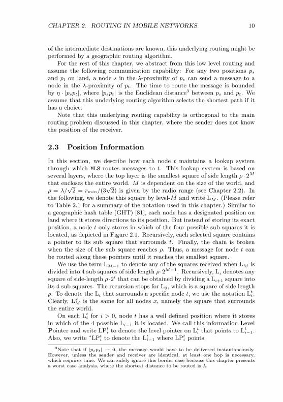
2.3 Position Information
In this section, we describe how each node t maintains a lookup systemthrough which MLS routes messages to t. This lookup system is based onseveral layers, where the top layer is the smallest square of side length ρ · 2Mthat encloses the entire world. M is dependent on the size of the world, andρ = λ/
√2 = rmin/(3
√2) is given by the radio range (see Chapter 2.2). In
the following, we denote this square by level-M and write LM . (Please referto Table 2.1 for a summary of the notation used in this chapter.) Similar toa geographic hash table (GHT) [81], each node has a designated position onland where it stores directions to its position. But instead of storing its exactposition, a node t only stores in which of the four possible sub squares it islocated, as depicted in Figure 2.1. Recursively, each selected square containsa pointer to its sub square that surrounds t. Finally, the chain is brokenwhen the size of the sub square reaches ρ. Thus, a message for node t canbe routed along these pointers until it reaches the smallest square.
We use the term LM−1 to denote any of the squares received when LM isdivided into 4 sub squares of side length ρ·2M−1. Recursively, Li denotes anysquare of side-length ρ·2i that can be obtained by dividing a Li+1 square intoits 4 sub squares. The recursion stops for L0, which is a square of side lengthρ. To denote the Li that surrounds a specific node t, we use the notation Lti.Clearly, LxM is the same for all nodes x, namely the square that surroundsthe entire world.
On each Lti for i > 0, node t has a well defined position where it storesin which of the 4 possible Li−1 it is located. We call this information LevelPointer and write LPti to denote the level pointer on Lti that points to Lti−1.Also, we write ∗LPti to denote the Lti−1 where LPti points.
3Note that if |pspt| → 0, the message would have to be delivered instantaneously.However, unless the sender and receiver are identical, at least one hop is necessary,which requires time. We can safely ignore this border case because this chapter presentsa worst case analysis, where the shortest distance to be routed is λ.

CHAPTER 2. ROUTING IN MOBILE NETWORKS 11
ρ · 2M
tLPtM−1
LPtM
LtM−1
LtM t
LPt1
LPt2
ρ
Lt2
Lt0 =∗LPt1
Lt1 =∗LPt2
Figure 2.1: The left figure shows the entire world surrounded by LM , thesquare of side length ρ · 2M . The land masses are filled with solid color(green), lakes are filled with waves. For each node t, Lti contains a levelpointer LPti that points to the sub square Lti−1 of size ρ · 2i−1 that containst. The right picture shows the smallest three levels around t and how eachlevel for i > 0 contains a pointer that points to the next smaller level.
We have seen that every node t stores a LPti on each of its levels Lti. Thisinformation needs to be hosted on a node somewhere in Lti. But because thenodes are mobile, we cannot designate a specific node on each Lti to storethe LPti. Therefore, we propose to store this pointer at a specific position pon land in Lti. Due to the minimal node density, we know that there existsat least one node in the λ-proximity of p, which we can use to store LPti. Ifthere are several nodes in the λ-proximity of p, we pick the one closest to p.The selected node then hosts LPti until it moves away from p by more than λ.At that point, it passes on LPti to its neighbor node closest to p, which mustexist due to the minimal node density. Over time, the LPti is not necessarilystored on the node closest to p, but by an arbitrary node in the λ-proximityof p.
Each node t stores a LPti at a well defined position pt on land within Lti,where pt is determined through the unique IDt of t. Any consistent hashfunction that maps the ID of a node onto a position on land can be used forthis purpose, as long as the chosen positions are evenly distributed over theland area for different IDs.
One possible function is the following, where we use two hash-functionsH1() and H2() to map the ID of t to real numbers in the range ]0, 1]. ptis determined as an offset (∆x,∆y) from the top left corner of Lti. ∆y is

CHAPTER 2. ROUTING IN MOBILE NETWORKS 12
Lti Level that contains t with side-length ρ · 2i(Lsi )
8 The 8 surrounding squares of LsiLPti Level pointer on Li for node t; points to Li−1∗LPti The Li−1 where LPti points to
δti distance of a node t to ∗LPti+1
FPti Forwarding pointer if LPti /∈ ∗LPti+1∗FPti The Li where ∗FPti points
TFPti Temporary forwarding pointer, before a pointer to t is removed∗TFPti The Li where TFPti points
TTLi Time to live of a TFPivnodemax Max. speed of nodes
rmin Min. communication range of a node
λ Min. distance to a node from any land point
ρ Side length of L0; ρ = λ/√
2 = rmin/(3√
2)
M LM surrounds the entire world
α When δti ≥ α · ρ · 2i, LPti+1 is updated
β(βT ) Max. number of forwarding hops to reach LPti from a FPti(TFPti)
γ See Lemma 2.4
η Routing overhead to route to a given position
Table 2.1: Nomenclature used throughout this chapter.
chosen such that, when only considering Lti, the fraction of land above ∆yis H1(IDt). Once ∆y is fixed, we must choose ∆x such that pt lies on land.We concatenate the line-segments where pt can be placed to a single line anddetermine ∆x such that the length of the line left to pt is H2(IDt) of thetotal line length.
Given this mapping, any node can determine the potential position ptwhere a node t might store a LPti for any Lti. All the node needs to knowis the ID of the receiver and the position of the lakes. Amongst others, thisis necessary to route a message along the level pointers towards t: Once amessage has been routed to a LPti, the node hosting LPti determines p′t in∗LPti and forwards the message to LPti−1, which is located at p′t.
We can already see that the number of levels only depends on the sizeof the deployment area and the transmission radius rmin. Therefore, everynode needs to maintain only a constant number of level pointers. Because thepositions of the level pointers are chosen randomly on the different levels, thestorage overhead is balanced smoothly on the nodes if the nodes themselvesare evenly distributed. This is an important property of MLS, and avoidsoverloading a few nodes with excessive amounts of data.

CHAPTER 2. ROUTING IN MOBILE NETWORKS 13
2.4 Lookup
Because messages are routed to a priori unknown positions, we denote themas lookup requests. When a sender node s wants to send a message to a des-tination node t, it issues a lookup request for node t, which encapsulates themessage to be sent. So far, we have described where each node publishes itslevel pointers and how a lookup request is forwarded along the level pointerstowards t once a first LPti has been found. This section is devoted to the firstphase of the lookup algorithm, which routes the lookup request to the firstLPti.
We propose a lookup algorithm that first searches t in the immediateneighborhood of s and then incrementally increases the search area until aLPti is found. From there, the lookup request can be routed towards thesmaller levels, as described in the previous section. Using this approach, wefind t quickly if it is close to s. In particular, we prove that the lookup timeis linear in the distance between s and t. As for the search areas, we use anextended version of the levels of node s, who issued the lookup request. Foreach Lsi , we define (Lsi )
8 to be the 8 Li squares adjacent to Lsi .In the very first step of a lookup, node s checks whether t is in its im-
mediate neighborhood. In this case, the message can be sent directly to t.Otherwise, the lookup request is sent to Ls1 to check whether it finds a LPt1.If this is not the case, the lookup request is forwarded in sequence to the 8squares of (Ls1)8, where it tries to find LPt1. This step is repeated recursively:while the lookup request fails to find a LPti on Lsi and (Lsi )
8, it is forwarded toLsi+1 and then in sequence to squares of (Lsi+1)8, where it tries to find LPti+1.A possible lookup path through the first 3 levels is depicted in Figure 2.2.Note that when the lookup request is forwarded through the levels of (Lsi )
8,the sequence is chosen such that the last visited Li is contained in Lsi+1, andthe request is always forwarded to a neighboring Li that shares an edge withthe current Li. (Skip Li that are completely covered by lakes.)
In the first phase of the lookup algorithm, the lookup request is routed toa series of levels Li, where it tries to find a level pointer LPti. In the followinglemma, we provide an upper bound for the time needed to search i levels.Note that this also gives an upper bound for the time needed to find LPti onLi, given that LPti ∈ Li.
Lemma 2.1. The accumulated time for searching a level pointer of node ton the levels 0 through i is bounded by η2i+1ρ(
√2 + 8
√5).
Proof. When a lookup request for node t issued by a node s starts its searchon Lj , it first queries for LPtj in Lsj . From the lookup algorithm presentedabove, we know that the lookup request tries4 to end its search of the lev-
4This fails, if Lsj−1 is the only sub-level of Lsj covering land. In this case, the lookup
request first needs to move into Lsj . This additional overhead is well compensated on the
previous level, where at least 3 Lsj−1 were not visited.

CHAPTER 2. ROUTING IN MOBILE NETWORKS 14
s
Figure 2.2: When s issues a lookup request for node t, the request is for-warded to the potential positions of a LPti in Lsi ∪ (Lsi )
8 for increasing i. Thebold gray squares in the left image indicate the first 4 levels of node s. Notethat we have only drawn the nodes visited by the chosen route. The rightimage shows a lookup path found by our simulation framework. The squaredots indicate the LP of the destination node. Because no lakes were presentin the lookup area, the lookup path is regular and draws quadratic shapes.
els Lj−1 on a node in Lsj . Thus, in the worst case, the request has to berouted over the diagonal of Lsj to reach the potential place of LPtj , which
implies a maximal route-time of η2jρ√
2. Then, to check for LPtj in (Lsj)8,
the lookup request is repeatedly sent to a neighboring Li to which the pre-vious Li shares an edge. At the worst, this takes η2jρ
√5 for each of the
8 neighbors. Thus, the total time to query for LPtj on level j is at most
η2jρ(√
2 + 8√
5), and the accumulated time to query i levels is bounded byt ≤
Pij=0 η2jρ(
√2 + 8
√5) < η2i+1ρ(
√2 + 8
√5).
Because LM is the same square for all nodes, we are sure that a lookuprequest finds a level pointer for t at the latest on LsM
5. In a later section,we give an upper bound on the time the lookup request needs to find a firstLPti based on the distance between s and t.
2.5 Lazy Publishing
In this and the following section, we analyze the implications of mobile nodes.In particular, this section focuses on the publish algorithm, through whichevery node keeps its level pointers up to date when it moves. Remember that
5This holds also under lazy publishing and in the concurrent setting, two conceptsthat are introduced in the following sections.

CHAPTER 2. ROUTING IN MOBILE NETWORKS 15
a b
LPti+2
LPti
LPti+1
LPti
LPti+1 LPti+1
αρ2i αρ2i
LPti+1
A B
B’A’
ρ2i t
Figure 2.3: If a node t oscillates between the two points a and b in the leftpicture, immediate updating of its level pointers would cause an enormousamount of traffic. In black are the level pointers necessary if t is at a, thelevel pointers necessary at b are gray. Lazy publishing delays the updatingof LPti+1 until node t has moved away from ∗LPti+1 by more than αρ2i, asdepicted in the right picture. Only when t moves across A, LPti+1 is updatedto A’. Similarly, only when t crosses B, A’ is deleted and B’ is added.
every node t maintains a LPti on each of its Lti for 0 < i ≤ M . Clearly, ifa node t must update its LPti+1 as soon as it changes Lti, the publish costmight be extremely high. The left part of Figure 2.3 depicts a situationwhere many level pointers would have to be updated due to an arbitrarilysmall move of node t. If t oscillates between the two points a and b, andimmediately sends messages to update the level pointers after moving an ε-distance, an enormous amount of traffic would be generated. To reduce thisoverhead, we employ lazy publishing, a concept that is similar to the lazyupdate technique utilized in [2].
Lazy publishing allows a node t to move out of ∗LPti+1 up to a certaindistance without updating LPti+1, and reduces the overhead due to oscillatingnodes. The following publish policy defines when a node t needs to updateits LPti.
We use the notation δti to denote the air distance of node t to ∗LPti+1.Formally, δti is the shortest distance of t to any edge of ∗LPti+1 if t /∈ ∗LPti+1.Otherwise, δti = 0.
Definition 2.2. (Publish Policy) When a node t has moved away from∗LPti+1 by more than α·ρ·2i, it needs to update LPti+1, such that LPti+1 pointsto the current Lti. Formally, a node t must update LPti+1 if δti ≥ α · ρ · 2i, fora fixed α ∈ R+.

CHAPTER 2. ROUTING IN MOBILE NETWORKS 16
We need to consider two cases while updating a LPti+1: If the outdatedLPti+1 is in Lti+1, it suffices to change the value of LPti+1 such that it points toLti. In the right half of Figure 2.3, this is the case when t moves over the linemarked A. However, if t has moved to a different Li+1, the outdated LPti+1
needs to be removed and a new one must be added to Lti+1. An example ofthis case is depicted in Figure 2.3, when t moves over the line marked B.
The implementation of such an update is straight forward: Node t sendsan update message to the outdated LPti+1 to change its value. If a new LPti+1
needs to be created, t sends a remove message to the outdated LPti+1 and acreate message to the position of the new LPti+1.
2.6 Concurrency
Clearly, the lookup algorithm presented in Chapter 2.4 does not supportlazy publishing in its second phase, where the lookup request follows thelevel pointers in order to find a destination node t. So far, we have assumedthat for i > 1, ∗LPti contains a LPti−1. However, under the lazy publishingpolicy, LPti−1 might be outside ∗LPti. We now derive modifications to thelookup and publish algorithms such that they support lazy publishing. Atthe same time, we introduce the issue of simultaneous lookup and publishrequests.
2.6.1 Forwarding Pointer
MLS uses a forwarding pointer to guide a lookup request to LPti. If LPti /∈∗LPti+1, ∗LPti+1 contains a forwarding pointer at the location where the LPtiwould be. This forwarding pointer points to the neighboring Li that containsLPti. In the following, we denote such a forwarding pointer by FPti and write∗FPti to denote the Li where FPti points. Figure 2.4 depicts a situation wherea FP is necessary. Note that we restrict the value of α to the range [0, 1[ suchthat a FPti might only point to an adjacent Li. This simplifies our analysis,but does not restrain the final result, where α is chosen clearly smaller than1 in order to maximize the allowed speed at which nodes may move.
With the forwarding pointers, a lookup request has an easy means to findthe LPti if LPti /∈ ∗LPti. However, this simplistic approach only works in astatic setup, where all publish requests of node t have terminated before alookup request queries for t. Consider again Figure 2.4 and suppose that tmoves upwards. When δti > αρ2i−1, t needs to send three messages: one toremove LPti from [C], one to add a new LPti in [D] and one to change thedirection of FPti in [B]. Because the messages might be delayed randomly bythe presence of lakes, it is possible that a lookup request reads FPti beforeit is updated, and then fails to find LPti in ∗FPti because LPti was alreadyremoved. This is a racing condition between a lookup request and the publishrequest which we need to avoid.

CHAPTER 2. ROUTING IN MOBILE NETWORKS 17
LPti
ρ2i
LPti+1
t
αρ2i
αρ2i−1
FPti
[A] [D]
[B] [C]
Figure 2.4: A node t is outside ∗LPti+1, but does not need to update LPti+1.Instead of removing its LPti in ∗LPti+1, t maintains a FPti that points to theneighboring Li there LPti can be found. When t moves upwards along theindicated (solid) path, it eventually leaves ∗LPti by more that αρ2i−1 andneeds to add a new LPti in [D], update FPti in [B] and remove the LPti in [C].To prevent a racing condition with a concurrent lookup, LPti in [C] is notremoved, but transformed to a TFPti that points to [D].

CHAPTER 2. ROUTING IN MOBILE NETWORKS 18
2.6.2 Temporary Forwarding Pointer
Inspired by the fact that the racing condition in the previous example arosebecause of a LPti that was removed too early, MLS does not remove LPtiimmediately, but leaves behind a Temporary Forwarding Pointer, denotedTFPti. Such a TFPti points to the neighboring Li where t was located whenit decided to remove the LPti. We will write ∗TFPti to denote the Li wherethe TFPti points.
To come back to Figure 2.4, t changes the LPti in [C] to a TFPti insteadof removing it. A lookup request that follows the outdated FPti then mightfind such a TFPti instead of the expected LPti and follows the TFPti to finallyfind LPti in [D].
At the time when LPti+1 is updated, the FPti in ∗LPti+1 becomes obsoleteand needs to be removed. But deleting the FPti could cause similar rac-ing conditions with a concurrent lookup request as when a LPti is removed.Therefore, MLS overwrites a FPti with a TFPti instead of removing the FPti.
According to its name, a TFP does only exist for a limited time. TFPare automatically removed after a given time, which we denote TTLi for aTFPti. Thus, the lifetime TTLi of a TFPti depends on the value of i. Wegive constraints on the value of TTLi while proving the correctness of MLS.Given that TTLi can be determined statically, a TFPti can be removed bythe hosting node without any interaction of node t.
2.7 The MLS Algorithm
We have now gathered all parts of MLS and present it here in a concise formbefore proving its correctness and performance. As before, the algorithmcomes in two parts, the publish and the lookup algorithm. The publishalgorithm is executed permanently by each moving node as to maintain validinformation on its hierarchy of levels, whereas the lookup algorithm is usedto route a message to a given node.
2.7.1 MLS Publish
During the startup phase of node t, initialize all level pointers LPti+1 to pointto Lti. While t is moving, it executes the protocol shown in Algorithm 2.1.In the initialization phase, t sends a message to the position of LPti on eachLi. This message tells the receiving node to store LPti, which points to Lti−1.We assume that there are no lookup requests for t during this initial phase.
While t is moving, it utilizes lazy publishing where it only performs anaction on level i if δti (its distance to ∗LPti+1) is above the given threshold(Line 1). If t updates LPti+1, FPti becomes obsolete and is changed to aTFPti that points to Lti (Line 2). The simplest case arises when only thevalue of LPti+1 needs to be changed, because LPti+1 can still point to the

CHAPTER 2. ROUTING IN MOBILE NETWORKS 19
Algorithm 2.1: Publish protocol of node t
if δti ≥ α · ρ · 2i then1
if i > 0 then change FPti in ∗LPti+1 to TFPti2
if LPti+1 ∈ Lti+1 then3
change LPti+1 to point to Lti4
else5
if LPti+1 ∈ ∗LPti+2 then6
change LPti+1 to FPti+1 that points to Lti+17
else if Lti+1 = ∗LPti+2 then8
change LPti+1 to TFPti+1 that points to Lti+19
else10
change LPti+1 to TFPti+1 that points to Lti+111
change FPti+1 to point to Lti+112
end13
on Lti+1, add LPti+1 that points to Lti14
end15
if i >0 and LPti /∈ Lti then16
add FPti on Lti that points to Li 3 LPti17
end18
end19
current Lti (Lines 3,4). This corresponds to the situation in the right part ofFigure 2.3 where t crosses A. Otherwise, LPti+1 is added to the current Li+1
of t (Line 14). In between, we update the forwarding pointers according tothe three different cases: (1) If the old LPti+1 is on the lookup-path becauseit is in ∗LPti+2, it is modified to a FPti+1 (Lines 6,7). (2) If t returned to∗LPti+2, we replace the old LPti+1 with a temporary forwarding pointer to∗LPti+2 (Lines 8,9). The FPti+1 in ∗LPti+2 is implicitly overwritten by Line 14.(3) In all other cases where t moves from one square to another in (∗LPti+2)8,we replace the old LPti+1 with a temporary forwarding pointer to the new Liand update FPti+1, which is located in ∗LPti+2 (Lines 11,12). Finally, if thenew LPti+1 does not point to the Li that contains LPti, a forwarding pointeris added to Lti. This FPti points to the Li that contains LPti (Lines 16, 17).This last case arises for example in Figure 2.4 when t moves along the dashedpath, such that the publish algorithm is triggered at the circled area. In thatcase, a FPti is added in square [D] and points to square [C], which holds LPti.
When t needs to update a pointer (LPti or FPti) on an arbitrary Li, t sendsa command message to the node that hosts the pointer, where the commandmessage indicates how the pointer should be modified. In order to createa new pointer on a Li, t sends a create message to the node closest to theposition pt in Li. If t sends a create message to set a LPti or FPti at positionpt, but there already exists a pointer (LPti, FPti or TFPti) at this position,the existing pointer is overwritten.

CHAPTER 2. ROUTING IN MOBILE NETWORKS 20
Algorithm 2.2: Lookup protocol of node s to route to node t
if t ∈ Ls0 ∪ (Ls0)8 then exit1
for i = 1; true; i++ do2
if P ti ∈ Lsi or P ti ∈ (Lsi )8 then3
p = P ti4
break5
end6
end7
Follow p until LPt1 is reached8
Route to a node closest to an arbitrary point on land in ∗LPt19
Forward to t10
2.7.2 MLS Lookup
A lookup request for node t issued by a node s is routed according to Algo-rithm 2.2. If the destination node t is in the same unit square or an immediateneighbor, node s and t can communicate directly over their radio. Becauses needs to know all its neighbors in Ls0 ∪ (Ls0)8 for routing, this situation canbe detected immediately and the lookup stops (Line 1).
Then, for increasing size of the levels, s searches a pointer of t in Lsiand then in the squares of (Lsi )
8. Note that the lookup request accepts anykind of pointer of node t, whether it is an LPti, FPti or TFPti. Furthermore,remember from Chapter 2.4 that the squares of (Lsi )
8 need to be accessed ina given order.
In the second phase of the lookup algorithm, the lookup request is routedalong the pointers until it reaches LPt1 (Line 8). Because ∗LPt1 does notcontain a LPt0, the lookup picks an arbitrary position p on land in ∗LPt1 androutes the lookup request to the node closest to p (Line 9). From that node,the lookup can be sent directly to t (Line 10).
2.8 Analysis
We devote this section to the analysis of MLS. In particular, we show thatMLS works in a concurrent setup, where publish requests and lookup requestsoccur simultaneously. We prove that a lookup request finds its destination inO(d) hops, where d is the distance between the sender and the destination.Also, we show that the amortized cost for publishing the position data isO(d log d), where d denotes the distance a node has moved. In order to provethese properties, we need to limit the maximum speed of nodes, denotedvnodemax . Throughout the proofs, we introduce different constraints on the valueof vnodemax . After proving the correctness of MLS, we determine the maximumnode speed that satisfies all these constraints.
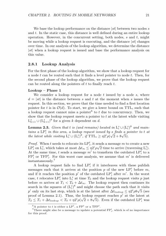
CHAPTER 2. ROUTING IN MOBILE NETWORKS 21
We base the lookup performance on the distance |st| between two nodes sand t. In the static case, this distance is well defined during an entire lookupoperation. However, in the concurrent setting, both nodes, s and t, mightbe moving while a lookup request is executing, and the distance |st| changesover time. In our analysis of the lookup algorithm, we determine the distance|st| when a lookup request is issued and base the performance analysis onthis value.
2.8.1 Lookup Analysis
For the first phase of the lookup algorithm, we show that a lookup request fora node t can be routed such that it finds a level pointer to node t. Then, forthe second phase of the lookup algorithm, we prove that the lookup requestcan be routed along the pointers of t to finally reach t.
Lookup – Phase 1We consider a lookup request for a node t issued by a node s, where
d = |st| is the distance between s and t at the moment when s issues therequest. In this section, we prove that the time needed to find a first locationpointer for t is in O(d). To start, we give a lower bound on TTLi such thata lookup request cannot miss a pointer6 to t due to concurrency. Then, weshow that the lookup request meets a pointer to t at the latest while visitingLsk+1 ∪ (Lsk+1)8 for a given k dependent on d.
Lemma 2.3. Given that t is (and remains) located in Lsi ∪ (Lsi )8 and main-
tains a LPti in this area, a lookup request issued by s finds a pointer to t atthe latest while visiting Lsi ∪ (Lsi )
8, if TTLi ≥ η2iρ(√
2 + 8√
5).
Proof. When t needs to relocate its LPti, it sends a message m to create a newLPti on Lti, which takes at most ∆tm ≤ η2iρ
√2 time to arrive (traversing Lti).
At the same time, t sends a message m′ to transform the outdated LPti to aFPti or TFPti. For this worst case analysis, we assume that m′ is deliveredinstantaneously.7
A lookup request fails to find LPti if it interleaves with these publishmessages such that it arrives at the position p of the new LPti before m,and if it reaches the position p′ of the outdated LPti after m′. In the worstcase, t relocates LPti into Lsi at time T0 and the lookup request visits p justbefore m arrives at T1 < T0 + ∆tm. The lookup request then continues itssearch in the squares of (Lsi )
8 and might choose the path such that it visitsp′ only on its last step, which is at the latest after ∆tlookup ≤ η2iρ8
√5 (see
proof of Lemma 2.1). Thus, the lookup request reaches p′ at the latest atT2 ≤ T1 + ∆tlookup < T0 + η2iρ(
√2 + 8
√5). Even if the outdated LPti was
6A pointer to t is either a LPt, a FPt or a TFPt.7There might also be a message to update a potential FPti, which is of no importance
for this proof.

CHAPTER 2. ROUTING IN MOBILE NETWORKS 22
transformed to a TFPti at T0, the TFPti exists at least until T0 + TTLi > T2
and the lookup request finds the TFPti. (Note that if the outdated LPti istransformed to a FPti, the time during which p′ hosts a pointer to t is evenlonger, because the FPti is transformed to a TFPti after t updates LPti+1.)
In the static case where publish requests and lookup requests do notinterfere, a lookup request finds a pointer to t at the latest while visitingLsk+1∪ (Lsk+1)8, if the side length of Lk is at least d (d ≤ ρ2k). (We can arguethat s ∈ Lsk+1 and thus t is at most d away from Lsk+1. At the same time,the distance from t to any Lk outside Lsk+1 ∪ (Lsk+1)8 is at least ρ2k ≥ d.Because α < 1, t must have created a LPtk+1 in Lsk+1 ∪ (Lsk+1)8.)
For the concurrent case, we weaken this result and show that the lookuprequest finds a pointer to t at the latest while visiting Lsk+γ ∪ (Lsk+γ)8, where
ρ2k ≥ d > ρ2k−1 and γ ∈ N+, if the maximum node speed is bounded by
vnodemax <1− α
2− 2−γ
η√
2(2.1)
and the temporary forwarding pointers exist long enough:
TTLi ≥ η2i+1ρ(1/√
2 + 8√
5) (2.2)
Note that increasing the value of γ results in a higher node speed, but alookup request might need to search longer until it finds a first pointer to t.We keep γ ≥ 1 as a parameter of MLS to tune its performance.
Lemma 2.4. Consider a lookup request for t issued by s and let d be thedistance |st| at the moment when the request is issued. For any γ ≥ 1,k ∈ N such that ρ2k−1 < d ≤ ρ2k, and if the Equations (2.1) and (2.2) hold,the lookup request finds a pointer to t at the latest on one of the levels inLsk+γ ∪ (Lsk+γ)8.
Proof. In a first step, we show that t has created a LPtk+γ in Lsk+γ ∪ (Lsk+γ)8
at the latest when the lookup request is issued. This property is necessaryto ensure that the lookup request cannot arrive too early on Lk+γ and missLPtk+γ because it is not yet created.
By definition, s ∈ Lsk+γ and thus t is at most d ≤ ρ2k away from Lsk+γ . Atthe same time, the distance from t to any Lk+γ−1 outside Lsk+γ∪(Lsk+γ)8 is at
least ρ(2k+γ−2k). Furthermore, we know that t sent off a message to create aLPtk+γ in Lsk+γ ∪ (Lsk+γ)8 when it entered this region by more than α2k+γ−1ρ
(lazy publishing). Thus, t moved at least a distance ∆d = ρ2k(2γ(1− α2
)−1)after sending off the message to create LPtk+γ and when the lookup requestwas issued.
At the limit, the update message to create LPtk+γ needs to be sent across
Lk+γ which needs ∆tupdate ≤ η2k+γρ√
2. But the lookup request is only

CHAPTER 2. ROUTING IN MOBILE NETWORKS 23
issued after t has moved ∆d, which takes at least ∆tmove ≥ ∆dvnodemax
. By
Equation (2.1), ∆tmove > η2k+γρ√
2 ≥ ∆tupdate, which shows8 that thelookup request is issued after a LPtk+γ has been created in Lsk+γ ∪ (Lsk+γ)8.
To conclude the proof, we show that a TFPtk+γ lives long enough to catchall cases where the lookup request does not find a LPtk+γ . From Lemma 2.3we know that the lookup request finds a pointer to t while t remains insideLsk+γ ∪ (Lsk+γ)8. Before t can relocate LPtk+γ outside Lsk+γ ∪ (Lsk+γ)8, it must
move at least ∆d′ = ρ2k(2γ(1 + α2
) − 1) after the lookup was issued, which
takes at least ∆t ≥ ∆d′
vnodemax> η2k+γρ
√2 by (2.1). Thus, t might create a
TFPtk+γ in Lsk+γ ∪ (Lsk+γ)8 at least ∆t after the lookup request was issued.By Lemma 2.1, the lookup request finishes visiting the levels of Lk+γ at
the latest after ∆tlookup ≤ η2k+γ+1ρ(√
2 + 8√
5). Thus, to ensure that theTFPtk+γ has not expired, it must have lived for at least ∆tlookup−∆t, whichholds by Equation (2.2).
The previous lemma states that a lookup request can find a pointer tot. We now show that the lookup request meets another pointer to t whenit is routed along a forwarding pointer (or temporary forwarding pointer).However, we need to restrain the maximum node speed to
vnodemax <α
η · 2(3√
2 + α)(2.3)
to ensure that this holds in all situations.
Lemma 2.5. A lookup request that finds a FPti or a TFPti also finds a pointerto t in ∗FPti or ∗TFPti, respectively, if the maximum node speed satisfiesEquation (2.3).
Proof. We need to show that [a] a pointer p′ for t has been written in ∗FPti(∗TFPti) before the lookup request following FPti (TFPti) arrives, and that[b] p′ cannot expire before the lookup request arrives, if p′ has been trans-formed to a temporary forwarding pointer. Let us denote the found FPti(TFPti) by p, the Li that contains p by A, and the Li where p points by B.Throughout the proof, we refer to the lines of the publish algorithm presentedin Chapter 2.7.1.
The found pointer p was created by one of the Lines 2, 7, 9, 11, 12, or 17.If p = TFPti was created by Line 2, it points to the Lti where t was locatedwhen t sent the message m to change the FPti to p. By the Lines 16-18, weknow that if B = ∗TFPti did not contain LPti, t sent a message m′ to createa FPti in B. If p = FPti was created by Line 17, B = ∗FPti contains LPti by
8Note that we did not consider that the lookup request needs some time to visitthe levels 1...k + γ − 1, because there are situations where this time is negligible small.Including this time would allow for a slightly better vnodemax , but unnecessarily complicatethe proofs.

CHAPTER 2. ROUTING IN MOBILE NETWORKS 24
definition. If p was created by Line 7, 9, 11, or 12, t sent a message m′ tocreate a LPti in B at the same time while sending a message m to create p.
Because t sends the message m′ to create the necessary pointer p′ in B nolater than m that creates p, the lookup request cannot arrive at the locationof p′ in B before m′. Otherwise, m′ would have been sent over a sub-optimalroute contradicting the triangle inequality. Therefore, condition [a] holds.
Consider the case where p is a TFPti and T0 is the time when t sentmessage m to crate p. Then, B (where p points) is the Li where t waslocated at T0, and B contains as p′ either a LPti or a FPti (Lines 14, 16-18).Because t is located in B at T0, it needs to move at least α2i−1ρ away fromB until p′ is changed to a TFPti. Also, at T0, t is at most α2iρ away fromA (Line 1), and therefore m arrives no later than T1 ≤ T0 + η2iρ(
√2 + α)
to create p = TFPti. At the limit, the lookup request reads p just beforeit expires at time T2 = T1 + TTLi, and then moves to p′ in B. Becausethe air-distance p− p′ is bounded by 2iρ
√8, the lookup request might arrive
at p′ no later than T3 ≤ T2 + η2iρ√
8 ≤ T0 + TTLi + η2iρ(3√
2 + α). Bythis time, p′ must not be expired, which requires that it was created afterT4 > T3 − TTLi. Before T4, t moved at most ∆d = (T4 − T0) · vnodemax . ByEquation (2.3), ∆d < ρ2i−1α, which shows that t has changed p′ to a TFPtiafter T4 and that p′ cannot expire before the lookup request arrives.
For the second case where p is a FPti, we use the fact that p is changedto a TFPti if t moves away from A by more than α · 2iρ (Lines 1,2), andtherefore an update message m′′ from t to p sent at T0 arrives at the latestat T1 ≤ T0 + η2iρ(
√2 +α). If t moves out of B and modifies p′ to a TFPti at
T0, it sends a message m′′ to p (Line 2 or 12). In the worst case, the lookuprequest reads p just before m′′ arrives and visits p′. Because the air distancep − p′ is bounded by 2iρ
√8, the lookup request arrives at p′ no later than
T2 ≤ T1 + η2iρ√
8 ≤ T0 + η2iρ(α + 3√
2). From Equation (2.2), we knowthat TTLi ≥ η2i+1ρ(1/
√2 + 8
√5). Because α < 1, p′ cannot expire before
the lookup request arrives.
We have shown that a lookup request can find a pointer to t and thatit can follow pointers to find new pointers. In the following, we give upperbounds on the time needed to find a LPti after a lookup request has beenrouted to an arbitrary FPti or TFPti. We tackle this problem by limitingthe maximum number of forwarding hops that the lookup request has tofollow until it reaches LPti. If the lookup request finds a FPti, we show thatit is routed to the corresponding LPti in at most β forwarding hops, if themaximum node speed is bounded by
vnodemax ≤α(β − 2)
2η(√
2 + α+ β√
8)(2.4)

CHAPTER 2. ROUTING IN MOBILE NETWORKS 25
and β > 2. If the lookup request finds a TFPti, we show that it is routed tothe corresponding LPti in at most βT forwarding hops, if the maximum nodespeed is bounded by
vnodemax ≤α2i−1ρ(βT − 2)
η2iρ(√
2 + α+ βT√
8) + TTLi(2.5)
and βT > 2. The values of β and βT become two additional tuning param-eters of MLS which influence vnodemax and the time a lookup needs to find itsdestination.
We will use the following helper lemma, which says that a node t needsto move at least a certain distance between consecutive updates to its LPti.
Lemma 2.6. Between successive updates to LPti, node t moves at least∆dupdate ≥ α2i−1ρ.
Proof. When a node t updates LPti, the new LPti points to Lti, the Li thatcontains t. Due to the publish policy (Definition 2.2), t only needs to updateLPti after it has moved out of Lti by α2i−1ρ and thus t must move at least∆dupdate before it needs to update LPti.
Lemma 2.7. Given a lookup request for a node t that has found a FPti, andthat vnodemax satisfies Equation (2.4), the lookup request can be routed to thecorresponding LPti in at most ∆t ≤ βη2iρ
√8 for a given β > 2.
Proof. Node t maintains FPti as long as δti < α2iρ (Lines 1,2 of the publishalgorithm in Chapter 2.7.1) and t does not return to ∗LPti+1 (Line 9). Whent updates its LPti, it also sends an update to FPti, which takes at most∆tupdate ≤ η2iρ(
√2 + α) time to arrive. When δti = α2iρ, t updates LPti+1
and changes the FPti to a TFPti (Line 2). Thus, when the lookup requestreads FPti, it reads a direction that is at most ∆tupdate outdated.
Consider the case where a node t moved from level X to Y and sent anupdate m to FPti, such that FPti points to Y instead of X. If a lookup requestreads FPti before m arrives, it first visits XY , where it finds a TFPti thatpoints to Y 9. By Lemma 2.5, this TFPti has not yet expired.
For each forwarding (FPti or TFPti), the lookup request has to move anair distance bounded by 2iρ
√8. Thus, the last lookup request relayed by X
arrives in Y at most ∆tupdate+2η2iρ√
8 after m was sent off. But during thistime, t might have moved - and left behind yet other (possibly temporary)forwarding pointers.
In order to limit the routing time to βη2iρ√
8, the lookup request canfollow at most β forwarding pointers until it reaches LPti. Thus, the totaltime between sending m and when the lookup request reaches LPti is ∆ttot ≤
9It is possible that ∗FPti does not contain a TFPti that points to Y . We discuss thiscase later on.
CHAPTER 2. ROUTING IN MOBILE NETWORKS 26
∆tupdate + βη2iρ√
8 ≤ η2iρ(√
2 + α + β√
8). During this time, t moves atmost ∆d ≤ ∆ttot ·vnodemax . By Equation (2.4), ∆d ≤ ρ(β−2)α ·2i−1 and causesat most ∆d/∆dupdate ≤ β − 2 additional forwarding pointers by Lemma 2.6.Including the two forwarding hops to visit X and Y , the lookup request hasto follow maximally β pointers, which takes at most βη2iρ
√8.
If ∗FPti does not contain a TFPti that points to Y , then t must havereturned to X and overwritten the TFPti with a LPti, a FPti or a more recentTFPti. Following such a FPti or TFPti short-cuts the path to LPti, and thelookup request finds LPti even faster.
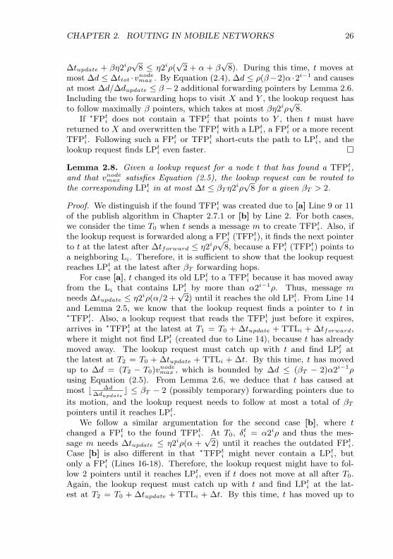
Lemma 2.8. Given a lookup request for a node t that has found a TFPti,and that vnodemax satisfies Equation (2.5), the lookup request can be routed tothe corresponding LPti in at most ∆t ≤ βT η2iρ
√8 for a given βT > 2.
Proof. We distinguish if the found TFPti was created due to [a] Line 9 or 11of the publish algorithm in Chapter 2.7.1 or [b] by Line 2. For both cases,we consider the time T0 when t sends a message m to create TFPti. Also, ifthe lookup request is forwarded along a FPti (TFPti), it finds the next pointerto t at the latest after ∆tforward ≤ η2iρ
√8, because a FPti (TFPti) points to
a neighboring Li. Therefore, it is sufficient to show that the lookup requestreaches LPti at the latest after βT forwarding hops.
For case [a], t changed its old LPti to a TFPti because it has moved awayfrom the Li that contains LPti by more than α2i−1ρ. Thus, message mneeds ∆tupdate ≤ η2iρ(α/2 +
√2) until it reaches the old LPti. From Line 14
and Lemma 2.5, we know that the lookup request finds a pointer to t in∗TFPti. Also, a lookup request that reads the TFPti just before it expires,arrives in ∗TFPti at the latest at T1 = T0 + ∆tupdate + TTLi + ∆tforward,where it might not find LPti (created due to Line 14), because t has alreadymoved away. The lookup request must catch up with t and find LPti atthe latest at T2 = T0 + ∆tupdate + TTLi + ∆t. By this time, t has movedup to ∆d = (T2 − T0)vnodemax , which is bounded by ∆d ≤ (βT − 2)α2i−1ρusing Equation (2.5). From Lemma 2.6, we deduce that t has caused atmost b ∆d
∆dupdatec ≤ βT − 2 (possibly temporary) forwarding pointers due to
its motion, and the lookup request needs to follow at most a total of βTpointers until it reaches LPti.
We follow a similar argumentation for the second case [b], where tchanged a FPti to the found TFPti. At T0, δti = α2iρ and thus the mes-sage m needs ∆tupdate ≤ η2iρ(α +
√2) until it reaches the outdated FPti.
Case [b] is also different in that ∗TFPti might never contain a LPti, butonly a FPti (Lines 16-18). Therefore, the lookup request might have to fol-low 2 pointers until it reaches LPti, even if t does not move at all after T0.Again, the lookup request must catch up with t and find LPti at the lat-est at T2 = T0 + ∆tupdate + TTLi + ∆t. By this time, t has moved up to

CHAPTER 2. ROUTING IN MOBILE NETWORKS 27
∆d = (T2−T0)vnodemax , which is bounded by ∆d ≤ (βT −2)α2i−1ρ using Equa-tion (2.5). From Lemma 2.6, we deduce that t has caused d ∆d
∆dupdatee ≤ βT−2
(possibly temporary) forwarding pointers due to its motion. (Note that weneeded to round up the number of forwarding pointers because t did notupdate LPti at T0.) Therefore, the lookup request needs to follow at most atotal of βT pointers until it reaches LPti.
We are now ready to assemble the first pieces of the puzzle and show thata lookup request finds a first LPt in bounded time.
Lemma 2.9. Given that vnodemax satisfies the Equations (2.1), (2.3), (2.4) and(2.5), and TTLi satisfies Equation (2.2) for fixed values of 0 < α ≤ 1, γ ≥ 1,β > 2, and βT > 2, then, a lookup request for node t issued by node s findsa level pointer LPt in O(d) time, where d is the distance |st| at the momentwhen the request is issued.
Proof. By combination of the Lemmas 2.4, 2.7, and 2.8: A first pointer p to tis found at the latest in one of the squares Lsu∪ (Lsu)8, where u = dlog2
dρe+γ
(Lemma 2.4). The necessary time the lookup request needs to visit all theselevels is bounded by T1 ≤ η2u+1ρ(
√2 + 8
√5) (Lemma 2.1). If p is a FPti, the
lookup request reaches the corresponding LPti in T2 ≤ βη2iρ√
8 (Lemma 2.7),and if p is a TFPti, the lookup request reaches the corresponding LPti inT3 ≤ βT η2iρ
√8 (Lemma 2.8). For T2 and T3, i ≤ u. The total time T to
find a first LPti is bounded by
T ≤ T1 + max(T2, T3)
≤ η2dlog2 (d/ρ)e+γ+1ρ(√
2 + 8√
5 + max(β, βT )√
2)
≤ d · η2γ+2(√
2 + 8√
5 + max(β, βT )√
2)| z constant
∈ O(d)
Lookup – Phase 2For the second phase of the lookup algorithm, we need to show that once
a lookup request has found a first LPti, it can follow the pointers and find thedestination node t. We start with another helper lemma stating that if LPtipoints to Li−1 and t is at most α2i−1ρ away from Li−1, then Li−1 containsa LPti−1 or a FPti−1.
Lemma 2.10. As long as δti < α2iρ, ∗LPti+1 contains a node that hostseither a LPti or a FPti.

CHAPTER 2. ROUTING IN MOBILE NETWORKS 28
Proof. By inspection of the publish algorithm presented in Chapter 2.7.1.The only places where pointers are transformed to TFPti are on the Lines 2,9 and 11. On Line 2, a FPti is removed, because LPti+1 will no longer pointto the level that contains the FPti. But this only happens when δti ≥ αρ2i
(Line 1).Line 9 or 11 is executed when δti−1 ≥ αρ2i−1. However, if Line 9 or 11
executes, we know from Line 6 that the LPtj that is overwritten is not in∗LPtj+1. We conclude that the pointer for t in ∗LPti+1 is transformed to aTFPti iff δti ≥ αρ2i.
The following lemma states that a lookup request that has reached a LPtican be routed along LPti and find LPti−1.
Lemma 2.11. Under the condition that i > 0, and all constraints on vnodemax
and TTLi are satisfied, a lookup request can follow LPti+1 and find LPti after∆t ≤ η2iρ
√8(1 + max(β, βT )).
Proof. First, we show that ∗LPti+1 contains a pointer p to t when the lookuprequest arrives. Then, we apply Lemma 2.7 and Lemma 2.8 to bound thetime to find LPti.
While δti < αρ2i, ∗LPti+1 contains a LPti or a FPti (by Lemma 2.10). AtT0, when δti ≥ αρ2i, the FPti in ∗LPti+1 is changed to a TFPti (Line 2 ofthe publish algorithm in Chapter 2.7.1) and a message m is sent to changeLPti+1, where it arrives at T1 ≤ T0 + η2iρ(α +
√8). A lookup request that
follows the outdated LPti+1 before m arrives reaches the TFPti in ∗LPti+1 atthe latest at T2 = T1 + η2iρ
√8 ≤ T0 + η2iρ(α + 4
√2). By Equation (2.2),
TTLi > T2−T0, and thus the TFPti does not expire before the lookup requestarrives.
So far, we have shown that the lookup finds a pointer to t in ∗LPti+1.Following LPti+1 to reach p takes at most η2iρ
√8. If p is a FPti, the additional
time to route to LPti is bounded by βη·2iρ√
8 (Lemma 2.7). If p is a TFPti, theadditional time to route to LPti is bounded by βT η2iρ
√8 (Lemma 2.8). Thus,
the total time to LPti is upper-bounded by ∆t ≤ η2iρ√
8(1+max(β, βT )).
Using the previous lemma, we can show that a lookup request can berouted from a LPti to LPti−1 until it reaches LPt1, from where it is forwardedto ∗LPt1. It remains to verify that the lookup request can be sent directly tot from within ∗LPt1, which we show under the constraint that
vnodemax <
√2− α
η(α+ 4√
2)(2.6)
Lemma 2.12. If vnodemax satisfies (2.6), a lookup request that has found LPt1can be sent directly to t from within ∗LPt1.

CHAPTER 2. ROUTING IN MOBILE NETWORKS 29
Proof. When t moves out of ∗LPt1 by more than αρ, it sends an updatemessage m to change LPt1 at time T0 (Definition 2.2). This message arrivesat T1 ≤ T0 + ηρ(α +
√8). A lookup request that reads LPt1 just before m
arrives, is forwarded to ∗LPt1. Because ∗LPt1 does not contain a LPt0, thelookup request is routed towards an arbitrary point on land in ∗LPt1, andmight end up on a node u that is up to λ away from ∗LPt1 (Lines 8-10 ofthe lookup algorithm in Chapter 2.7.2). At the limit, this forwarding to urequires to traverse Lt1, and the lookup request arrives at u at T2 ≤ T1+ηρ
√8.
By this time, t has moved ∆d ≤ (T2 − T0)vnodemax < ρ(√
2− α) and is at most∆d+αρ ≤ λ away from ∗LPt1. Both, u and t are at most λ away from ∗LPt1,and the diameter of ∗LPt1 is ρ
√2 = λ. Thus, the total distance between
u and t is at most 3λ = rmin, which shows that u can forward the lookuprequest directly to t.
Theorem 2.13. (Lookup) Given that vnodemax satisfies the Equations (2.1),(2.3), (2.4), (2.5), and (2.6), and that TTLi satisfies the Equation (2.2) forfixed values of 0 < α ≤ 1, γ ≥ 1, β > 2, and βT > 2, then, a lookup requestfor a node t issued from a node s takes O(d) time to reach t, where d = |st|is the distance between s and t when the request is issued.
Proof. By Lemma 2.9, we know that the time to find a first level pointeris bounded by T1 ≤ d · η2γ+2(
√2 + 8
√5 + max(β, βT )
√2) Also, we know
that this first level pointer is found at the latest on level dlog2dρe+ γ. From
Lemma 2.11, we deduce that following the level pointers from level dlog2dρe+
γ downto 1 takes
T2 ≤dlog2 d/ρe+γX
j=1
η2jρ√
8(1 + max(β, βT ))
and the time to forward the lookup request from LPt1 to t can be boundedusing Lemma 2.12 to
T3 ≤ ηρ√
8(1 + max(β, βT ))
The total time until the lookup request reaches t is therefore bounded by
Tlookup ≤ T1 + T2 + T3
≤ T1 +
dlog2 d/ρe+γXj=0
η2jρ√
8(1 + max(β, βT ))
< T1 + dη2γ+2√
8(1 + max(β, βT ))
≤ d · η2γ+2(3√
2(1 + max(β, βT )) + 8√
5)| z constant
∈ O(d)

CHAPTER 2. ROUTING IN MOBILE NETWORKS 30
2.8.2 Maximum Node Speed
While proving the lemmas in the previous section, we formulated constraintson the value of vnodemax and TTLi. In this section, we collect all of theseconstraints and present the maximum node speed for which MLS is provento work. The value of TTLi only needs to satisfy Equation (2.2). Becauseenlarging TTLi implies a reduction of vnodemax by Equation (2.5), we chooseTTLi as small as possible:
TTLi = η2i+1ρ(1/√
2 + 8√
5) (2.7)
To determine the maximum vnodemax , we need to fix the parameters 0 < α <1, β > 2, γ ≥ 1 and βT > 1. The value of η is given indirectly by the topologyand the underlying routing algorithm. While maximizing vnodemax , we opt tominimize Tlookup, the worst case time of a lookup request, which dependson the same parameters. Thus, we need to determine α, β, γ and βT , suchas to maximize vnodemax and minimize Tlookup under the constraints that theEquations (2.1), (2.3), (2.4), (2.5) and (2.6) are satisfied.
For γ → ∞; β → ∞, βT → ∞, we receive that vnodemax ≈ 0.0845η
forα ≈ 0.863. This is an unreachable upper bound, because the maximum costof a lookup request would grow to infinity. Clearly, there is a tradeoff be-tween maximizing vnodemax and minimizing Tlookup. The higher we choose themaximum node speed, the longer is the worst-case time of a lookup request.But while Tlookup increases exponentially with γ, the value of γ barely in-creases vnodemax . Similarly, β and βT have an impact on vnodemax while they arebelow 20, higher values only increase Tlookup. Twiddling the parameters, wefound γ = 1, β = 5, and βT = 19 to optimize the tradeoff between vnodemax
and Tlookup. Using these values, vnodemax becomes maximal for α = 0.8. Wecan now state our lower bound on the maximum node speed for which MLS isproven to work.
Theorem 2.14. For α = 0.8, β = 5, βT = 19 and γ = 1, the nodes mightmove at speed vnodemax ≤ 1
15·η without breaking MLS.
Proof. By plugging the parameters into the Equations (2.1), (2.3), (2.4),(2.5) and (2.6).
In the absence of lakes, 1/η can be interpreted as the minimum speed atwhich messages are routed by the underlying routing algorithm. Therefore,the above result shows that nodes might move at a speed that is only 15times smaller than the routing speed, which is remarkably fast. If we considerreal-world nodes such as the mica2 nodes from UC Berkeley, a data packetexperiences around 50 ms delay while being forwarded by a node. Thus, apacket can be sent about 40 hops per second. If we assume that a message isforwarded around 10 meters per hop, the message speed reaches around 400meters per second. In this setup and in the absence of lakes, the maximum
CHAPTER 2. ROUTING IN MOBILE NETWORKS 31
node speed is bounded by 400/16 = 25 meters per second (90 km/h, about 56mph), which exceeds by far the node speed in typical network applications.
2.8.3 Publish Analysis
Last but not least, we need to consider the cost of the publish algorithm.While a node is moving, it continuously sends updates onto its different levels.This produces messages that need to be routed by the nodes of the system.Thus, bounding the message overhead of the publish algorithm is of criticalimportance to ensure that the overall routing cost induced by the movingnodes is reasonable. First, we derive the maximum cost of publishing to alevel. Then, we determine the amortized message cost for publishing while anode is moving.
Until now, we made use of an underlying routing algorithm that candeliver a message to its destination in η·d time, when the air distance betweenthe sender and destination is d. For the following, we assume that the numberof routing hops needed to send a message over a distance d is proportional tothe routing time and write η ·d to denote the number of routing hops neededto route a message to a target that is d away.
Lemma 2.15. The cost to publish on level-i is bounded by η2i+2ρ(√
8 + α)message-hops.
Proof. By inspection of the publish algorithm in Chapter 2.7.1. We deter-mine the message cost c of each individual line to pick the execution withmaximum cost.
On Line 2, FPti is in the neighboring level-i, which t just left by morethan α · 2i, thus c2 ≤ η2iρ(α +
√2). For the Lines 4, 7, 9, and 11, the
distance from t to LPti+1 is maximally 2i(α +√
8) and the message cost isc4,7,9,11 ≤ η2iρ(α +
√8). FPti+1 on Line 12 is contained in (Lti+1)8, but
only as long as δti+1 < α2i+1. Thus, the cost to send a message to FPti+1 isbounded by c12 ≤ η2iρ(2α +
√8). For Line 14, LPti+1 is contained in Lti+1,
and therefore the cost is c14 ≤ η2iρ√
8. Finally, for Line 17, t reaches FPti inc17 ≤ η2iρ
√2 hops, as FPti ∈ Lti. The execution with maximum cost visits
the Lines 2, 11, 12, 14 and 17. Summing up the corresponding costs resultsin the indicated number of hops.
Using an amortized analysis, we can now show that the expected messageoverhead induced by the publish method can be bounded.
Theorem 2.16. (Publish)The amortized message cost of a node induced by the publish method is at
most O(d log d) message hops, where d denotes the distance the node moved.

CHAPTER 2. ROUTING IN MOBILE NETWORKS 32
Proof. A node t updates its LPti when δti−1 ≥ αρ2i−1 (Definition 2.2). Afteran update to LPti, t ∈ ∗LPti and thus t needs to move at least αρ2i−1 beforeit needs to issue another update for LPti (Lemma 2.6). Therefore, t needs toupdate LPti at most d/(αρ2i−1) times while moving a distance d. The cost topublish on Li is maximally η2i+2ρ(
√8 +α) (Lemma 2.15), and the total cost
for updating Li while moving the distance d is bounded by dη8ρ(√
8 +α)/α.The total publish cost is given by the sum of the cost of each level to whicht has to publish. Because ∀j : δtj = 0 after the initialization phase of thepublish method, t only needs to publish on Li if d ≥ αρ2i−1, and the totalpublish cost is bounded by d log2(2d/α)η8ρ(
√8 + α)/α ∈ O(d log d). Note
that the total number of levels is M (Chapter 2.2) and the publish cost isfurther bounded by dMη8ρ(
√8 + α)/α.
2.9 Simulation
We support our theoretical results with a series of simulations, through whichwe show that the average lookup time and publish cost are well below theworst case costs. Our simulation framework implements mobile nodes thatselect their route using the random waypoint model and maintain their hi-erarchical lookup data according to Chapter 2.7.1. However, being mainlya proof of concept, the simulation abstracts from the underlying routing10,where we delay messages according to the route length, but do not simulatethe node-to-node routing. Also, we simulate only a (random) sub-set of thenodes as to improve the run-time. As a consequence, the storage of pointersis performed by the framework and relieves us from ensuring the minimumnode density.
The techniques of Le Boudec et al. [61] to obtain a stationary regimecannot be applied, because the nodes are not memoryless with respect totheir lookup hierarchy. Therefore, we obtain a close to stationary regimethrough a long first phase, during which each node moves at least to itsfirst waypoint before any lookup request is issued. Afterwards, the nodesissue lookup requests to randomly chosen nodes, where each node only sendsanother lookup request when the previous request arrived.
We ran the simulation with 5000 nodes issuing a total of 100000 lookuprequests and repeated it for different node speeds and two different worldmaps. Map1 corresponds to the world shown in Figure 2.1. The maximalrouting stretch due to lakes is 10, the side-length is 5300 units and ρ waschosen to be 1 unit. Map2 is of the same size, but contains no lakes atall. The average lookup stretch is shown in the left plot of Figure 2.5. Forincreased node speed (1 corresponds to vnodemax ), nodes produce more TFP,which helps lookup requests to find a first pointer to their destination, which
10Remember that the underlying routing can route a message to a given position. Thisis orthogonal to our main goal, where the location of the destination node is unknown.
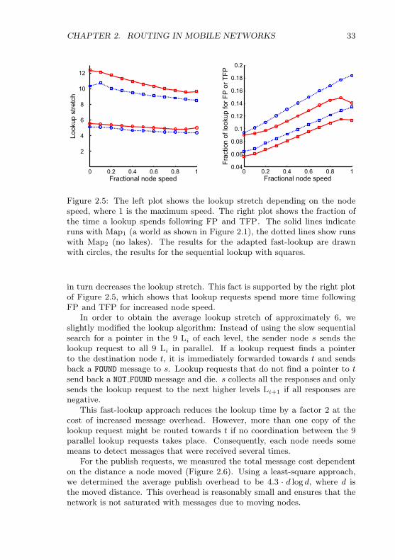
CHAPTER 2. ROUTING IN MOBILE NETWORKS 33
0 0.2 0.4 0.6 0.8 1
2
4
6
8
10
12
Fractional node speed
Look
up s
tretc
h
0 0.2 0.4 0.6 0.8 10.04
0.06
0.08
0.1
0.12
0.14
0.16
0.18
0.2
Fractional node speed
Frac
tion
of lo
okup
for F
P o
r TFP
Figure 2.5: The left plot shows the lookup stretch depending on the nodespeed, where 1 is the maximum speed. The right plot shows the fraction ofthe time a lookup spends following FP and TFP. The solid lines indicateruns with Map1 (a world as shown in Figure 2.1), the dotted lines show runswith Map2 (no lakes). The results for the adapted fast-lookup are drawnwith circles, the results for the sequential lookup with squares.
in turn decreases the lookup stretch. This fact is supported by the right plotof Figure 2.5, which shows that lookup requests spend more time followingFP and TFP for increased node speed.
In order to obtain the average lookup stretch of approximately 6, weslightly modified the lookup algorithm: Instead of using the slow sequentialsearch for a pointer in the 9 Li of each level, the sender node s sends thelookup request to all 9 Li in parallel. If a lookup request finds a pointerto the destination node t, it is immediately forwarded towards t and sendsback a FOUND message to s. Lookup requests that do not find a pointer to tsend back a NOT FOUND message and die. s collects all the responses and onlysends the lookup request to the next higher levels Li+1 if all responses arenegative.
This fast-lookup approach reduces the lookup time by a factor 2 at thecost of increased message overhead. However, more than one copy of thelookup request might be routed towards t if no coordination between the 9parallel lookup requests takes place. Consequently, each node needs somemeans to detect messages that were received several times.
For the publish requests, we measured the total message cost dependenton the distance a node moved (Figure 2.6). Using a least-square approach,we determined the average publish overhead to be 4.3 · d log d, where d isthe moved distance. This overhead is reasonably small and ensures that thenetwork is not saturated with messages due to moving nodes.

CHAPTER 2. ROUTING IN MOBILE NETWORKS 34
Figure 2.6: We captured over 600000 node motions during our simulation.This figure shows the publish overhead caused by a moving node plottedagainst the distance the node moved. The (least-square) average is indicatedwith the dashed line.
3Routing in 3D Networks
We have seen that the geographic routing approach is very scalable as it isbased solely on local information. In the preceding chapter, we have describeda lookup system through which messages can even be delivered to nodes thatare constantly moving. But all results we have seen so far are valid onlyfor 2-dimensional networks. In this chapter, we examine how the geographicrouting technique needs to be adapted to reliably deliver messages in 3-dimensional networks. In contrast to the previous chapter, however, we onlyconsider the simpler case of static networks.
Clearly, messages can still be greedily forwarded towards their destina-tion, which is likely to work fine in dense networks. But the recovery fromlocal minima becomes more challenging, as the faces surrounding the networkhole now expand in two dimensions and are much harder to capture. We showin Chapter 3.6.1 that it is indeed possible to describe the surface of networkholes using only local information. Our approach is quite different from 2Das there is no equivalent to the planarization of a graph in 3D. Furthermore,we used the right/left hand rule in 2D to route along the 1-dimensional face,but there is no simple analogon in 3D to visit all nodes delimiting the surfaceof a hole. In fact, Durocher et al. have proved that there is no determinis-tic local routing algorithm for 3D networks that guarantees the delivery ofmessages if the nodes are not allowed to store any message state [30]. Asan immediate consequence, there is neither a local memoryless algorithm totraverse all nodes on a given surface in a deterministic manner.
The proof in [30] has two parts: First, the authors show that the existenceof a k-local1 geographic routing algorithm for UBG implies the existenceof a 1-local geographic routing algorithm for any connected graph. In thesecond part, they show that any deterministic 1-local routing algorithm can
1A k-local routing algorithm can base its routing decision on a k-neighborhood of thecurrent node.

CHAPTER 3. ROUTING IN 3D NETWORKS 36
be defeated, disproving the existence of a k-local routing algorithm. In fact,even very simple graph structures do not allow for deterministic routingalgorithms.
In the sequel, we present memoryless and local geographic routing pro-tocols for 3-dimensional networks and compare them to other routing tech-niques. Unlike the deterministic greedy-face-greedy solutions in 2D, our ap-proach applies a randomized recovery to lead messages out of local minima.
3.1 Random Walks
The non-existence of local, memoryless routing algorithms that delivermessages deterministically [30] has many direct and indirect consequences.Whereas it is possible to deterministically traverse a planar subdivision andreport all nodes and faces [12], there is no corresponding algorithm in 3D.However, it has been shown in [27] that for any undirected graph, it is pos-sible to assign each node a local ordering of its edges such that a routingalgorithm can visit all nodes in O(n) time (deterministically!) by leaving anode through the edge succeeding the edge through which it entered. Unfor-tunately, the construction of the local edge-orderings requires a global viewof the graph and has construction time cubic in the number of nodes. Thegreedy geographic routing we would like to apply to our 3D graphs is actuallyclose to optimal - as long as the messages do not get stuck at local minima.But as there is also no deterministic recovery algorithm that could lead themessages out of local minima, we need to fall back to randomized recoverytechniques which we describe breifly in this section.
A message moving around randomly in a network may seem very ineffi-cient and too simplistic, but there is quite some work in this area indicatingthat random walks need not be as bad as it looks at a first glance. The twoprominent models to capture a random walk on a graph G = (V,E) are (1)the Markov chain, and (2) the flow in an electrical network obtained from Gby replacing every edge by a resistance of 1Ω. See [68] for a survey of thetopic. In the following, we use n := |V | and m := |E|.
For our purpose, the hitting time Huv, and the cover time CG turn outto be most interesting. Huv is the expected time until the random walk firstvisits vertex v when starting its walk at u, and CG is the expected timeneeded to visit all nodes of G at least once. For arbitrary graphs, we haveCG = O(n ·m) = O
`n3´
[9], which poses also an upper bound on Huv. Thecomplete graph has optimal cover time Θ(n logn), and the worst cover timeof Θ
`n3´
is obtained from the lollipop graph [38]. The 2D mesh has a non-optimal cover-time O
`n log2 n
´, whereas the 3D mesh has optimal cover-time
O(n logn) [20]. Using the electrical resistance approach, the cover time ofan arbitrary graph can be bounded to CG ≤ 2mRspan [20], where Rspan isthe minimum resistance of a spanning tree in G. Since Rspan ≤ n − 1 for

CHAPTER 3. ROUTING IN 3D NETWORKS 37
any graph, we obtain that CG ≤ 2m(n− 1). The hitting time Huv seems tobe intrinsically difficult to capture, but the somewhat related commute timeκuv, the expected time to travel from u to v and back again, can be expressedby Huv < κuv = 2mRuv, where Ruv is the effective resistance between u andv [20].
A random geometric graph is obtained by placing n nodes uniformly atrandom in the unit square and connect two points if their distance is at mostr. The minimal value of r such as to obtain a connected graph is subject of
the percolation theory. It has been shown that if r ≥ rcon = Θ“p
logn/n”
,
the graph is connected w.h.p. [78]. Random geometric graphs with r ≥√8rcon have optimal cover time of O(n logn) [5]. Whereas this model seems
appealing for wireless networks at the first moment, we need to keep inmind that the analysis only holds for n → ∞. Furthermore, a connectedrandom geometric graph requires so many network nodes that the graphtends to have no routing voids at all, causing no local minima to the greedyrouting algorithm. In addition, wireless networks are obviously not randomgeometric graphs: There tend to be many holes in the network, where nonodes are deployed, which is ignored completely in this model.
3.2 Notation and Model
We now summarize the notation used to describe our 3D routing protocolsbefore we show a lower bound on the routing stretch of any local routingalgorithm in 3D. Whereas this lower bound applies for arbitrary graphs, werestrict our attention to unit ball graphs in Chapter 3.5. Unit ball graphs(short UBG) are the 3D equivalent to the unit disk graphs in 2D, and con-stitute a basic model for wireless networks where we assume that any twonetwork nodes are connected iff their distance is below a certain thresh-old rmax, the maximal transmission radius2. W.l.o.g. we will assume thatrmax = 1 unit. As usual, we describe the network as a graph G = (V,E),where V is the set of network nodes, and E the set of connections betweennodes. The number of nodes is denoted by n := |V |, and the number of edgesby m := |E|. Furthermore, we use the notation Sr(v) to denote the sphereof radius r around a given node v, and the set of neighbors of a node v isabbreviated by N (v).
3.3 Lower Bound
We start by deriving a lower bound for the performance of geographic routingalgorithms in 3 dimensions. The following theorem states that any random-
2We are aware that a UBG is a very simplistic model for wireless networks, where thetransmission range is far from circular. Our main routing techniques presented in thiswork, however, are valid for real wireless networks.

CHAPTER 3. ROUTING IN 3D NETWORKS 38
ized geographic routing algorithm has at least a cubic stretch. (This lowerbound would also hold for deterministic algorithms, which we know to notexist at all.)
Theorem 3.1. Let d be the length of the optimal path between a given sourceand destination in a 3-dimensional network. There are networks for whichthe route found by any randomized geographic routing algorithm has expectedlength Ω
`d3´.
Proof. The proof idea is similar to the lower bound for 2-dimensions pre-sented in [60]. We consider the following family of networks: For a positiveinteger r, construct a 3-dimensional graph as shown in Figure 3.1: Firstplace nodes on the surface of a sphere with radius r such that the mutualdistance between any two nodes is at least 2. Obtain a first set of surface-nodes from S1 := (r · sin(2i · arcsin(1/r)), 0, r · cos(2i · arcsin(1/r))) | i ∈[0, b0.5π/ arcsin(1/r)c]. In Figure 3.1, these nodes are drawn as solid squareson the left boundary of the sphere. The remaining surface points, also drawnas solid squares, are obtained from this initial set: For each (x, y, z) ∈ S1, add(x · sin(2i · arcsin(1/x)), x · cos(2i · arcsin(1/x)), z) | i ∈ [1, bπ/ arcsin(1/x)c]to an initially empty set S2. As a second step, add intermediate nodes on thesurface (drawn as small diamonds) that connect nearby surface nodes. (Themath is nearly the same as for the surface nodes and is omitted.) Further-more, append to each surface-node a line of b(r− 1)/2c nodes. The distancebetween nodes on the line is 1, and the line is directed towards the center ofthe sphere. These line-nodes are represented with round (red colored) dotsin Figure 3.1. Finally, select an arbitrary surface node w, and append to itsline further nodes until the center of the sphere, node t, is reached.
Note that there is no edge between nodes on different lines, as the linesare mounted on surface-points at least 2 units apart, and the length of thelines is less than r/2. Furthermore, the number of points per line is Θ(r). Todetermine the number of surface nodes, we use (a) α/2 < arcsin(α) < 2α,and (b) sin(α) > α/2 for α ∈ [0, 1]. For a surface-node in S1 with a given x-coordinate, the number of surface-nodes added to S2 is bπ/ arcsin(1/x)c > xfor x ≥ 1.4, using (a). Thus, we can bound |S2| by summing up the valuesof the x-coordinates of the nodes in S1 using (a) and (b):
|S2| ≥ 2 ·
12
jπ
2 arcsin(1/r)
kXi=1
r · sin(2i · arcsin1
r) ≥
r/2Xi=1
i ∈ Θ`r2´ .
The total number of nodes in the graph is (|S1|+ |S2|) ·Θ(r) = Θ`r3´.
We now route from an arbitrary node s on the surface to node t in thecenter of the sphere. An optimal routing algorithm routes along the surfaceuntil it hits w and then follows the line until it reaches t. The path on thesurface consists of at most 2.5 surroundings of the sphere, requiring O(r)

CHAPTER 3. ROUTING IN 3D NETWORKS 39
w
t
Figure 3.1: Lower bound graph for geographic routing algorithms. Nodesrepresented by solid squares lie on the surface of a sphere with mutual dis-tance at least 2. Nodes printed as diamonds lie also on the surface andconnect these points. The round (red colored) nodes lie on lines leading fromthe surface-nodes towards the center. A single dedicated surface-node w hasan extended line leading to node t in the center of the sphere. This imagewas created with sinalgo, our simulator for network algorithms described inChapter 7.
hops. The line contains at most r nodes to traverse, which results in a totalcost of O(r) hops for the optimal algorithm.
A geographic routing algorithm, on the other hand, needs to find thesurface-node w on whose line-end the destination node t is located. Since onlylocal routing information is available, this can only be achieved by exploringthe lines by descending from the surface-nodes until t is found. For anyrandomized routing algorithms, the adversary can attach the line leading tot to a random surface-node, requiring the algorithm to explore Ω
`r2´
linesuntil it finds t, which requires Ω
`r3´
hops, which shows that the expectedrouting stretch is at least cubic.

CHAPTER 3. ROUTING IN 3D NETWORKS 40
3.4 Towards 3D Routing Algorithms
For our geographic routing algorithm, we use a greedy-random-greedy ap-proach, short GRG, where the message is forwarded greedily until a localminimum is encountered. To resolve local minima, a randomized recoveryalgorithm kicks in. Unlike the deterministic face-routing in 2D, there is nodeterministic recovery algorithm for 3D networks [30]. Therefore, our recov-ery technique is bound to be randomized.
Of course, the recovery part also needs to be memoryless and local, whichimmediately rules out flooding techniques3 which could quickly find a nodecloser to the destination than the local minimum. We propose to use randomwalks (short RW), which constitute a very simple, yet surprisingly efficientrecovery technique. We apply the following four techniques to ensure theperformance of random walks:(1 ) Region Limited Random Walks: When applying a RW to escape a localminimum at node u, the message is likely to explore large parts of the entirenetwork until hitting a node v which is closer to the target than u, requiringO(n ·m) hops. In most cases, however, such an extensive exploration is notneeded: Let v be the node closet to u such that v is closer to the target thanu, and let k be the length of the shortest path connecting u and v. Then,exploring Sk(u) with a RW would have been sufficient in order to find v. Asthe value of k is not known, the recovery algorithm performs an exponentialsearch by limiting the RW in sequence to S2i(u) with i ∈ 2, 3, . . . until anode closer to the target is found. For each sphere of radius r, the recoveryalgorithm performs O
`r6´
RW hops, which corresponds to the cover time forthe sparse subgraph contained in the sphere, bounding the recovery cost toO`k6´
hops (see Theorem 3.5).(2 ) RW on the surface: Similar to the face routing in 2D graphs, we canfurther restrict the RW to nodes delimiting the hole which causes the localminimum and which needs to be surrounded. Chapter 3.6.1 describes howthe nodes can locally determine the surface in a UBG, using the dual graphof Chapter 3.5.(3 ) Sparse Subgraph: We have seen that for arbitrary graphs, Huv =2mRuv < 2mn, and CG ≤ 2mRspan < 2mn. Both Huv and CG grow linearlyin m and n, and we can improve Huv and CG by removing nodes in denseregions, and any edge that is not critical for the connectivity of the graph.We can achieve both points relatively easy by performing the RW on a con-nected dominating set, e.g. see [94], which implicitly also reduces the numberof edges. Similarly, topology control algorithms build sparse subgraphs con-sidering the network characteristics, and tend to be more stable [83, 97]. A
3Needless to say that we could implement a memoryless flooding algorithm whereeach node rebroadcasts a message whenever its TTL permits to do so, allowing multipletransmissions from the same node. However, such a scheme comes with an impracticaloverhead growing exponentially with the TTL.
CHAPTER 3. ROUTING IN 3D NETWORKS 41
truly sparse subgraph could be obtained by limiting the RW to an arbitraryspanning tree, reducing CG and Huv to 2n2. But as a spanning tree cannotbe constructed locally, this approach is rather impractical for unstable net-works. The dual graph presented in 3.5 is not only sparse, but also also fulfillsthe property that any Sr(u) contains at most O
`r3´
dual nodes, limiting thecover time of a RW restricted to Sr(u) to O
`r6´.
(4 ) Power of choice for RW: The cover time of a RW can be improved bynot returning to the previous node, if applicable. I.e. when the message issent from n to m, and if n is not the only neighbor of m, then m forwards themessage to a random neighbor, but not n. This improvement derives fromthe power of choice for RW [6].
3.5 Dual Graph
We now describe the construction of a dual graph eG = (eV , eE) of G = (V,E),on which our routing schemes are based. The position of the dual vertices(short DV ) is bound to the intersection points of a regular cubic (imaginary)grid, covering the entire space. The DV are only placed nearby networknodes in order to populate the grid in regions where G is present. EachDV is owned by exactly one nearby network node, relating eG to G. Therelation from G to eG is a bit more involved, as the relation is not bijective.In order to switch from a node v ∈ V to eG, v chooses the DV d closest to v.We will see that d is owned by either v or a neighbor of v.
Edges in eG are only present between direct neighbors in the underlyinggrid. The dual graph is defined such that the connectivity of G is preservedin eG. I.e. a path between eu, ev ∈ eV in eG implies a path in the original graphbetween own(eu) and own(ev), where own(x) denotes the owner of x. Similarly,a path between u, v ∈ V in G implies a path between the correspondingDV in eG. As a result, we can perform a virtual routing on eG, and executethe corresponding routing steps on G. Finally, eG is sparse in the sense thateach d ∈ eV has constant out-degree, and ‖eV ‖ is linear in the volume ofSv∈V S1(v), the volume G occupies. In the remainder of this section, we
show the following theorem:
Theorem 3.2. eG is a sparse, connectivity preserving virtual graph of G,which can be constructed locally.
The construction of eG consists of the following two steps. First, eachnode determines the set of DV it owns. Then, the edges eE are added to eGsuch that two DV are connected iff they are direct neighbors in the virtualgrid: (x1, x2) ∈ eE ⇔ ‖x1x2‖ = η, where η denotes the cell-side-length ofthe grid, whose value we determine in Chapter 3.5.2. This step basicallyrequires each node to determine all neighboring DV owned by other nodes.

CHAPTER 3. ROUTING IN 3D NETWORKS 42
Algorithm 3.1: Construction of G (Code for node v)
Ownership Selection1
foreach(DV d ∈ Sρ(v))2
if(@u ∈ N (v) s.t. u.ID < v.ID∧‖ud‖ ≤ ρ)3
v selects d as RDV4
foreach(u ∈ N (v))5
S := DV d | dist(d, vu) ≤ h ∧ ‖vd‖ < ‖ud‖6
remove from S all DV already known to be RDV7
TDV= TDV ∪ S8
send TDV to N (v)9
drop multi-owned DV if v.ID > ID of other owner10
Connect11
send(RDV ∪ TDV ) to 3-hop neighborhood of v12
Determine the edges adjacent to any owned DV13
The construction of eG is completely local, and each of the network nodesonly knows a very limited local view of eG at any time.
3.5.1 Ownership Selection
The DV are positioned only on specific positions in space, defined by theintersection points of a regular cubic grid. The set of possible positions for aDV is given by (iη, jη, kη) | i, j, k ∈ N. Our algorithm will ensure (locally!)
that at most one DV is added to eV for any of these positions.The ownership selection algorithm executed by each node v ∈ V deter-
mines for each node the set of DV v owns, see Algorithm 3.1. It consists oftwo substeps. First, v determines its regular dual vertices (short RDV ), forwhich v can determine statically whether it owns them (Lines 2–4). Nodev chooses as RDV all DV which are most ρ away from v. In addition, forevery selected RDV d, v may not have a neighbor u with a lower ID, whosedistance to d is bounded by ρ. Formally, the set of RDV of node v is d | dis a DV ∈ Sρ(v) ∧ @u ∈ N (v)(u.ID < v.ID ∧d ∈ Sρ(u)). The exclusion ofsome nodes based on their ID is to ensure that each DV is owned by exactlyone network node. In Figure 3.2, the sphere with radius ρ around v denotesthe region where v selects its RDV. The value of ρ at least as large as toensure that Sρ(v) contains at least one DV, further information about ρ isgiven in Chapter 3.5.2. Please note that if a node v ∈ V does not own anyRDV, then the DV ∈ Sρ(v) are owned by (direct) neighbors of v.
The second substep of the ownership selection ensures connectivity in thedual graph by adding additional DV to eG. In contrast to the first substep,there may be several nodes v ∈ V that decide to own the same DV. The reso-lution of these conflicts is straight forward, but requires communication withthe 1-hop neighborhood in G. Therefore, each node calls the DV selected

CHAPTER 3. ROUTING IN 3D NETWORKS 43
in this substep tentative dual vertices (short TDV ). To ensure connectivity,the TDV depend on the neighborhood N (v) of node v. For each neighboru, node v determines all DV at most h =
√3η/2 away from the line vu and
closer to v than to u4. Then, v selects as TDV only the DV which it doesnot already own (as RDV or TDV ), and are not already known to be regu-larly owned by a direct neighbor (Lines 5–8). Figure 3.2 depicts the regionwhere node v chooses its TDV with a cylinder enclosing the line vu. Foreach RDV node v keeps, it also remembers the reason, i.e. the node u dueto which the RDV was considered in the first place.
For the removal of multiple owners for the same TDV introduced inthis second step, each node v sends its TDV list to its neighbors (Line 9).Assume v selects TDV d due to its neighbor u, and also another node nchoose d. Again, we resolve the conflict using the IDs, and let the lowerID win. Assume w.l.o.g. that n.ID < v.ID. Then, v needs to learn that itshould drop its ownership of d. The value of η, and therefore the value of h,is chosen such that in such a situation, either (a) n ∈ N (v) or (b) n ∈ N (u),see Chapter 3.5.2 for more details. In case (a), v receives the TDV list from ndirectly and therefore learns about n’s ownership of d. In the second case (b),u receives the TDV lists from both, v and n, and u can detect the conflict.u then determines whether u was v’s reason for the conflicting TDV d, andif n /∈ N (v). If (and only if) both conditions hold, u sends a withdraw(d)message to v, indicating that v should not own d.
After this second substep is completed, each DV (RDV and TDV ) is sureto have exactly one owner v ∈ V . When the DV are connected as describedin the introduction of this section, we are ready to state a first connectivityproperty of eG: If there is a path between two nodes v1, v2 ∈ V , there alsoexists a path between d1, d2 ∈ eV , where di is the closest DV to vi. Thisproperty follows directly from Lemma 3.3, which is formulated for a singlehop in G.
Lemma 3.3. Given two neighboring nodes (v1, v2) ∈ E and two dual vertices
d1, d2 ∈ eV s.t. di is the closest DV to vi, we can ensure that d1 and d2 areconnected in eG by adding to eV all DV at most h =
√3η/2 away from the
line ` = v1v2.
Proof. Because the side length of the grid is η, we know that the di themselvesare at most h away from vi. This forms the base-case of our inductive proof.As for the induction step, we consider a point P that moves along ` from v1
to v2, and a DV x which is at most h away from `. Let Q be the positionof P when P leaves Sh(x). We show that when P moves out of Sh(x), thereis a DV x′ whose distance to Q is strictly smaller than h, and that x′ isconnected to x in eG.
4In case of equal distance, the node with smaller ID may own the DV.
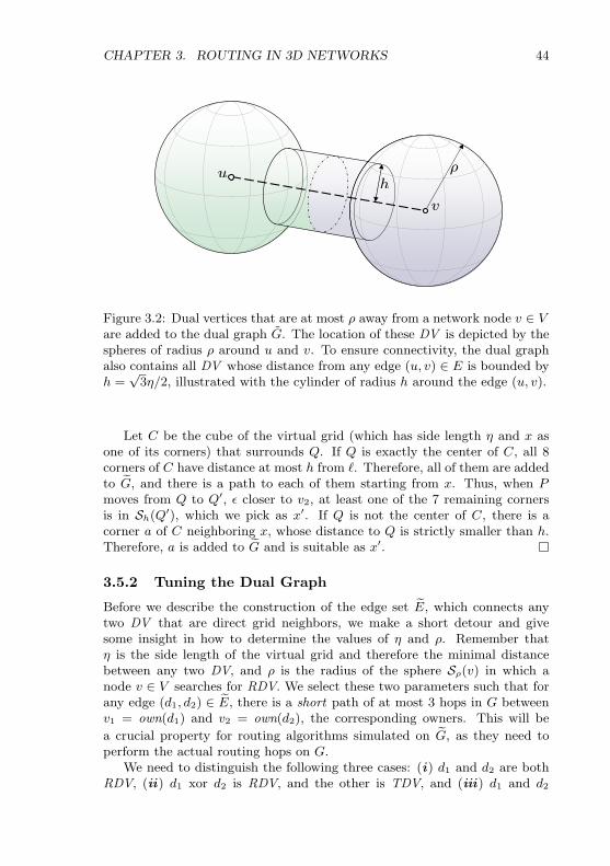
CHAPTER 3. ROUTING IN 3D NETWORKS 44
v
u
h
ρ
Figure 3.2: Dual vertices that are at most ρ away from a network node v ∈ Vare added to the dual graph G. The location of these DV is depicted by thespheres of radius ρ around u and v. To ensure connectivity, the dual graphalso contains all DV whose distance from any edge (u, v) ∈ E is bounded byh =√
3η/2, illustrated with the cylinder of radius h around the edge (u, v).
Let C be the cube of the virtual grid (which has side length η and x asone of its corners) that surrounds Q. If Q is exactly the center of C, all 8corners of C have distance at most h from `. Therefore, all of them are addedto eG, and there is a path to each of them starting from x. Thus, when Pmoves from Q to Q′, ε closer to v2, at least one of the 7 remaining cornersis in Sh(Q′), which we pick as x′. If Q is not the center of C, there is acorner a of C neighboring x, whose distance to Q is strictly smaller than h.Therefore, a is added to eG and is suitable as x′.
3.5.2 Tuning the Dual Graph
Before we describe the construction of the edge set eE, which connects anytwo DV that are direct grid neighbors, we make a short detour and givesome insight in how to determine the values of η and ρ. Remember thatη is the side length of the virtual grid and therefore the minimal distancebetween any two DV, and ρ is the radius of the sphere Sρ(v) in which anode v ∈ V searches for RDV. We select these two parameters such that forany edge (d1, d2) ∈ eE, there is a short path of at most 3 hops in G betweenv1 = own(d1) and v2 = own(d2), the corresponding owners. This will be
a crucial property for routing algorithms simulated on eG, as they need toperform the actual routing hops on G.
We need to distinguish the following three cases: (i) d1 and d2 are bothRDV, (ii) d1 xor d2 is RDV, and the other is TDV, and (iii) d1 and d2

CHAPTER 3. ROUTING IN 3D NETWORKS 45
are both TDV. From the ownership selection algorithm, we deduce that themaximal distance of a RDV from its owner is ρ.
In the first case (i), there should be an edge (d1, d2) ∈ eE only if (v1, v2) ∈E, requiring (a) 2ρ + η < 1. Otherwise, it could happen that the pathbetween v1 and v2 is of length O(|V |), which we wanted to avoid. For (ii),assume w.l.o.g. that d1 is a TDV selected by v1 due to its connection withr1 (the reason for d1), and that d2 is a RDV. Then, the distance from v2 tod1 is at most ρ+η, and the distance from v2 to v1r1 is bounded by ρ+η+h.By requiring (b) ρ+ η+ h ≤
√3/2, we ensure that v2 ∈ S1(v1)∪S1(r1), and
that v2 is a neighbor of either v1 or r1. As a result, we can route from v1
to v2 either directly, or via r1. For (iii), where vi choose di as TDV due to
a node ri, there should be an edge (d1, d2) ∈ eE only if v1 or r1 is neighborof at least one of v2 or r2: (N (v1) ∪ N (r1)) ∩ (v2 ∪ r2) 6= ∅. Otherwise, itcould again happen that the path between v1 and v2 requires O(|V |) hops.Assume the situation where (N (v1) ∪ N (r1)) ∩ (v2 ∪ r2) = ∅. Then, d2 canbe placed closest to v1r1 if ‖v1r1‖ = ‖v2r2‖ = 1 and if v2 and r2 are placedon S1(v1) ∩ S1(r1). Then, the minimal distance between the two lines v1r1
and v2r2 is 1/√
2. As the di may be placed h away from their corresponding
line, we need that (c) 1/√
2− 2h > η s.t. (d1, d2) /∈ eE. Thus, if (d1, d2) ∈ eE,this constraint ensures that there is a route from v1 to v2, either directly orvia r1 and r2, requiring at most 3 hops.
Our goal is to maximize η such that ‖ eE‖ is as small as possible. Consider-ing condition (c), we need to choose h as small as possible. In Chapter 3.5.1,we have seen that h =
√3η/2 satisfied our requirements. In fact, choosing
h any smaller could break the connectivity of eG. Using (c), we deduce thatη < 1/(
√2+√
6). As for ρ, we would like to choose its value as large as possi-ble to maximize the number of statically determinable RDV. Constraint (a)yields ρ=0.37 for η=0.258, which also satisfies condition (b). We have justshown the following lemma:
Lemma 3.4. Given two DV d1, d2 from the dual graph, and vi = own(di),
the corresponding owners of the di. Then, if (d1, d2) ∈ eE, i.e. the distancebetween d1 and d2 is η, there is a path from v1 to v2 in G of at most 3 hops.
Proof. The lemma is satisfied by setting the values of η, ρ and h as describedabove.
3.5.3 Connecting the Dual Graph
In the remainder of this section, we describe the construction of the edgeset eE. The dual edges connect any two DV which are direct grid neighbors,which limits the outdegree of any DV to 6. For our local construction, thismeans that the owner own(d) = v of a DV d needs to determine which of the

CHAPTER 3. ROUTING IN 3D NETWORKS 46
Algorithm 3.2: RW step (On node v, previous node p, Sr(s))
if(target ∈ (v ∪N (v))) v or one of its neighbors is the target1
deliver the message and return2
if(number of hops for this sphere-size has been performed)3
r = 2r Increase the sphere delimiting the region of the RW4
N := set of owners of N (v) s.t. ∀n ∈ N : ‖ns‖ ≤ r5
Only select the owners which are in Sr(s)
if(N = p) RW can only return to p, no choice6
send message to p7
else Apply “power of choice”8
send message to random node in (N \ p)9
6 potential neighbors of d exist. For each existing neighbor n, v determinesthe owner own(n), and the path over which own(n) can be reached in G.
We know from Lemma 3.4 that the owner own(n) is at most 3 hopsaway from v. Therefore, it is sufficient if each node broadcasts5 the set ofDV it owns to its 3-hop neighborhood (Line 11 of Algorithm 3.1). Alongthe broadcasting path, every node that forwards the message can add itsown ID, such that the receiver can easily determine the path (in G) to reachthe sender. Please note that any node owns only O(1) DV, and thereforethe storage overhead to remember the local view of the dual graph does notexceed the desired size.
Finally, we have seen all the pieces to state the proof of Theorem 3.2:
Proof of Theorem 3.2. From the ownership selection algorithm we deducethat the maximal distance between any DV and its owner is below 1. Withother words, a network node v ∈ V only owns DV that lie in S1(v). Thus,
any u ∈ eV lies in Q =Sv∈V S1(v). As the volume Q is composed of spheres
of radius 1, there are no arbitrarily thin areas in Q, and we can concludethat Q contains O(Q) DV. In combination with the fact that the outdegree
of any DV is at most 6, this shows that eG is sparse.The connectivity of the dual graph eG is an immediate consequence of
Lemma 3.4 and Lemma 3.3, and an algorithm to construct eG locally hasbeen presented in this section.
5Broadcasting from a node v to its 3-hop neighborhood can be implemented quiteefficiently without retransmissions in the following way: The message contains a TTLcounter initially set to 3 and a variable s storing the sender v. Upon reception of amessage m at node u, u first decrements the TTL. Then, u rebroadcasts the messageonly if the following three conditions hold. TTL > 0, m.s 6= u, and m.s /∈ N (u) ifTTL = 1.

CHAPTER 3. ROUTING IN 3D NETWORKS 47
3.6 Routing on the Dual Graph
Our simplest routing scheme, called pureRW, performs region limited randomwalks (see Chapter 3.4) until it finds the target. The spheres delimiting theregions to explore are centered at the sender node, and the random walkapplies the “power of choice” technique. Note that pureRW does not performany greedy routing steps at all.
The RW selects its next hop based on the sparse dual graph eG, the se-lection algorithm is described in Algorithm 3.2. If the sender node s doesnot own any DV itself, it first sends the message to its neighbor which ownsthe DV closest to s. (The existence of such a neighbor is given, see Chap-ter 3.5.1.) We use the following additional notation: For a node v, let v.DV
denote the set of DV owned by v, and eN (v) the set of DV which are neigh-boring a DV in v.DV, excluding the ones owned by v itself.
The number of random hops for a sphere of radius r is O`r6´, the cover
time of the nodes contained in the sphere. The routing stretch of pureRW canbe bounded as following:
Theorem 3.5. Let Sopt be the stretch of the optimal geographic routing al-gorithm for 3D graphs. The expected stretch of pureRW is O
`Sopt
2´.
Proof. For any source-target pair (s, t), let k be the length of the optimalroute between s and t, and j the smallest integer s.t. 2j ≥ k. pureRW performsa RW limited to S2i(s) for i ∈ 2, 3, . . . , j. For any sphere of radius r, itperforms O
`r6´
random hops, which results in a total of O`k6´
random hops.As any optimal algorithm has cubic stretch requiring O
`k3´
hops in the worstcase (Theorem 3.1), the stretch of pureRW is O
`Sopt
2´.
Clearly, pureRW is not a practical routing scheme as its expected deliverytime is just as bad as its stretch. Therefore, we try to route much moreoptimistically using the GRG approach, at the cost of that we are unable toanalytically express its performance.
The greedy routing step of the GRG routing scheme selects the DV ineN (v) closest to the target and forwards the message to its owner (Line 3 ofAlgorithm 3.3). Initially, if the sender s of the message does not own anyDV, it sends the message to its neighbor which owns the DV closest to s.The message is greedily forwarded until the target is found (Line 2), or alocal minimum is reached (Line 5).
The recovery algorithm chosen by the GRG is either the region limitedRW described in Algorithm 3.2, or a region limited RW that is also boundto the surface of the hole which needs to be surrounded.

CHAPTER 3. ROUTING IN 3D NETWORKS 48
Algorithm 3.3: Dual Greedy Step (On node v)
if(target ∈ (v ∪N (v))) v or one of its neighbors is the target1
deliver the message and return2
select d ∈ (N (v) ∪ v.DV ) closest to the target3
if(d is owned by v) v is in a local minimum for the target4
start recovery5
else6
send message to own(d)7
3.6.1 Routing on the Surface
We describe the surface of a hole in the network with the aid of the virtual 3Dgrid introduced in Chapter 3.5. The surface S is described by a list of grid-cubes which delimit the boundary between the hole and the network. Eachnode has only its local view of S, which it determines using the presence,respectively absence of DV.
When the greedy routing described in Algorithm 3.3 reaches a local min-imum at node v (Line 5), the DV d closest to the target is owned by v itself.Therefore, at least one of the 6 grid-neighbors of d is not present, otherwise,d would not be closest to the target. Let i be the non-present grid-neighborwhich is closest to the target, i.e. i is an intersection point of the grid neigh-boring d, where no DV was placed. Then, the four grid-cubes delimited bythe cube-edge di are part of the surface S. The remaining grid-cubes describ-ing v’s view of S are obtained iteratively: Until S does not change anymore,v does the following for every grid-cube q ∈ S: For every corner c of q forwhich v owns the corresponding DV, v determines c1, c2, c3, the three cor-ners adjacent to c on q. For each ci, v adds to S the 4 grid-cubes delimitedby the cube-edge cci iff no DV was placed on ci. When the iteration stops,S contains the grid-cubes delimiting the surface around the local minimum,as seen by v.
Let SN (v) be the set of owners which own a DV lying on the cornerof a grid-cube q ∈ S, and exclude v from SN (v). This set describes theneighbors of v which also lie on the surface S, and from which the RW picksan arbitrary node to forward the message to. If node v decides to forwardthe message to u ∈ SN (v), it needs to describe the surface to u. It does soby including each q ∈ S which has a corner owned by u. Upon receiving themessage, u sets its initial view S of the surface to this subset and determinesthe remaining grid-cubes describing u’s view of the surface by applying theiterative algorithm described above.
Thus, the description of the surface changes constantly, but remainsstrictly local. In fact, when v sends the surface description to u, it is possiblethat u determines yet more grid-cubes which touch DV of v as well. Thiscan happen when the surface S touches v in two or more independent places,

CHAPTER 3. ROUTING IN 3D NETWORKS 49
such that v cannot determine locally the relationship. In situations whereu is the only node that knows that the surface bends back to v, we needto ensure that u sends its view of the surface to v from time to time. Butthis requires that we drop the ‘power of choice” optimization presented inChapter 3.4. Otherwise, we risk falling into an infinite loop, as the RW maynot explore the entire surface.
3.7 Simulation
In order to validate our geographic routing algorithms for 3D networks, weperformed a series of simulations in Sinalgo, our Java-based simulation frame-work for testing and validating network algorithms described in Chapter 7.We chose a fairly large simulation area of 20 × 20 × 10 units and deployedbetween 2000 and 40000 nodes to cover the range between very sparse anddense networks. In order to obtain more realistic networks, we first placed100 randomly rotated and randomly positioned cuboids of 2× 2× 1 units inthe simulation area. The cuboids were areas where no node could be placed,and they enforced holes in the network, such that, especially for dense net-works, the messages could not be forwarded greedily without surroundingany holes.
Sparse graphs tend to be heavily twisted, which challenges our GRGrouting algorithms with many local minima. To account for this fact, weperformed more simulations for sparse networks, which can also be seen bythe accumulation of samples for small n in Figure 3.3. For each initial de-ployment of n nodes, we first connected the nodes to a UBG, and kept onlythe giant component, the largest connected part of the network.
For each network, we selected 5000 random sender/target node pairs (s, t)and sent a message from s to t using the following five recovery algorithmswhen the message got stuck in a local minimum: RW on the dual, RW onthe surface, RW on the Graph, bounded DFS on a spanning tree, and abounded flooding. All RW were limited to exponentially growing regions(see Chapter 3.4), and all but the RW on the surface implemented the powerof choice technique. The bounded DFS on an arbitrary spanning tree isnot a local algorithm and was chosen for comparison. In that algorithm,we first built a spanning tree, and then perform a DFS on the tree, wherethe maximal depth to explore the graph increases exponentially. Finally,we implemented a recovery algorithm that uses flooding to escape a localminimum. The flooding relies on a mark-bits to avoid repetitions of themessage, and is thus not memoryless. The TTL of the flooding message wasincremented exponentially to obtain an optimal search time.
Figure 3.3 compares the overhead (measured in routing hops) of the fiverecovery algorithms. For ease of interpretation, we plotted against the over-head of the flooding algorithm, such that the y-axis shows how much more

CHAPTER 3. ROUTING IN 3D NETWORKS 50
0
2
4
6
8
10
12
14
16
18
0 5000 10000 15000 20000 25000 30000 35000 40000
Number of deployed nodes (n)
RW Graph
RW Dual
DFS Tree
RW Surface
Routi
ng o
verh
ead c
om
pare
d t
o f
loodin
g
Figure 3.3: The overhead of our routing techniques compared against a non-memoryless flooding algorithm. The x-axis indicates how many nodes weredeployed, the y-axis how much more routing-messages our routing algorithmsinduced.
overhead the other routing algorithms induced.A first important observation is that limiting the RW to the surface of
the hole does in fact not help at all. Unless the network is very dense, ittends to have a single huge face covering nearly the entire network. I.e. theholes in the network are nearly never completely closed and most of themare interconnected over the surface. As a result, the restriction to the facedoes not reduce the number of nodes to visit.
We can further observe that the overhead of the RW on the dual is belowthe overhead of the RW on the graph, which shows that we achieved our goalsof obtaining a sparse network graph via the dual graph. The astonishinggood performance of the DFS on the spanning tree for the sparse networkscan be traced back to the fact that the nodes of these networks have verylow degree, resulting in a tree-like network. For denser networks, however,the RW approaches perform much better. In particular, the RW on the dualand the RW on the surface perform even better than the flooding for verydense networks, as they operate on a sparser network.
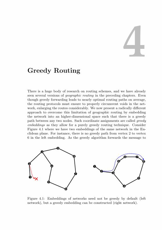
4Greedy Routing
There is a huge body of research on routing schemes, and we have alreadyseen several versions of geographic routing in the preceding chapters. Eventhough greedy forwarding leads to nearly optimal routing paths on average,the routing protocols must ensure to properly circumvent voids in the net-work, enlarging the routes considerably. We now present a radically differentapproach to overcome this limitation of geographic routing by embeddingthe network into an higher-dimensional space such that there is a greedypath between any two nodes. Such coordinate assignments are called greedyembeddings as they allow for a purely greedy routing technique. ConsiderFigure 4.1 where we have two embeddings of the same network in the Eu-clidean plane. For instance, there is no greedy path from vertex 2 to vertex6 in the left embedding. As the greedy algorithm forwards the message to
1
2
3
9
4
5
6
1
23
9
88
7
4
5
6
7
Figure 4.1: Embeddings of networks need not be greedy by default (leftnetwork), but a greedy embedding can be constructed (right network).
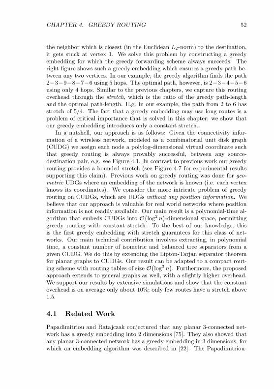
CHAPTER 4. GREEDY ROUTING 52
the neighbor which is closest (in the Euclidean L2-norm) to the destination,it gets stuck at vertex 1. We solve this problem by constructing a greedyembedding for which the greedy forwarding scheme always succeeds. Theright figure shows such a greedy embedding which ensures a greedy path be-tween any two vertices. In our example, the greedy algorithm finds the path2−3−9−8−7−6 using 5 hops. The optimal path, however, is 2−3−4−5−6using only 4 hops. Similar to the previous chapters, we capture this routingoverhead through the stretch, which is the ratio of the greedy path-lengthand the optimal path-length. E.g. in our example, the path from 2 to 6 hasstretch of 5/4. The fact that a greedy embedding may use long routes is aproblem of critical importance that is solved in this chapter; we show thatour greedy embedding introduces only a constant stretch.
In a nutshell, our approach is as follows: Given the connectivity infor-mation of a wireless network, modeled as a combinatorial unit disk graph(CUDG) we assign each node a polylog-dimensional virtual coordinate suchthat greedy routing is always provably successful, between any source-destination pair, e.g. see Figure 4.1. In contrast to previous work our greedyrouting provides a bounded stretch (see Figure 4.7 for experimental resultssupporting this claim). Previous work on greedy routing was done for geo-metric UDGs where an embedding of the network is known (i.e. each vertexknows its coordinates). We consider the more intricate problem of greedyrouting on CUDGs, which are UDGs without any position information. Webelieve that our approach is valuable for real world networks where positioninformation is not readily available. Our main result is a polynomial-time al-gorithm that embeds CUDGs into O
`log2 n
´-dimensional space, permitting
greedy routing with constant stretch. To the best of our knowledge, thisis the first greedy embedding with stretch guarantees for this class of net-works. Our main technical contribution involves extracting, in polynomialtime, a constant number of isometric and balanced tree separators from agiven CUDG. We do this by extending the Lipton-Tarjan separator theoremfor planar graphs to CUDGs. Our result can be adapted to a compact rout-ing scheme with routing tables of size O
`log3 n
´. Furthermore, the proposed
approach extends to general graphs as well, with a slightly higher overhead.We support our results by extensive simulations and show that the constantoverhead is on average only about 10%; only few routes have a stretch above1.5.
4.1 Related Work
Papadimitriou and Ratajczak conjectured that any planar 3-connected net-work has a greedy embedding into 2 dimensions [75]. They also showed thatany planar 3-connected network has a greedy embedding in 3 dimensions, forwhich an embedding algorithm was described in [22]. The Papadimitriou-

CHAPTER 4. GREEDY ROUTING 53
Ratajczak conjecture was settled by Moitra and Leighton [72] who presenta polynomial-time algorithm for constructing a greedy embedding of a given3-connected planar graph. In this chapter, we study the embedding of acombinatorial UDG where only the connectivity information but no positioninformation of the vertices is given. The absence of such geometrical informa-tion eliminates the possibility of planarizing the network and using a triangu-lation technique. The embedding of a UDG in combination with routing hasbeen studied widely [16, 43, 80, 86], but none of these approaches guaranteesa greedy embedding. In fact, finding an exact embedding is NP-hard [14]and cannot be approximated arbitrarily well [58]: If non-neighboring ver-tices must have a distance larger than 1, it can be shown that there maybe neighbors with distance
p3/2. The best known approximation algorithm
for this problem is described in [77] and may induce distances in O`log2.5 n
´.
Even if each vertex knows the exact distance to any of its neighbors or theexact angles at which the neighbors are located, the problem of finding anexact embedding remains NP-hard [4, 16].
As a way of avoiding these difficulties and finding embeddings for CUDGs,anchor based routing was introduced, e.g. [37, 41, 96]. The main idea of theserouting schemes is that a few vertices are elected as anchor nodes and eachvertex stores the length of its shortest path to all anchor nodes. The set ofthese distances can be seen as a virtual coordinate on which greedy routingcan be applied. To ensure a greedy embedding, however, Θ(n) anchors needto be chosen in the worst case [96], which renders this approach unattractive.
Kleinberg proposed a greedy embedding of arbitrary networks into thehyperbolic plane [52], which was improved by Eppstein et al. such thatcoordinates of the embedding only need O(logn) bits [33]. As of this writing,such greedy embeddings into hyperbolic space are only known for trees, i.e.given a general network, only a spanning tree thereof is embedded. Thereduced connectivity information of a spanning tree has severe consequencesfor the routing performance: Close-by vertices in the network may be far awayon the tree on which the routing takes place, introducing a linear worst-casestretch. To the best of our knowledge, we present the first greedy embeddingwith guaranteed sublinear stretch. For CUDGs, a generalization of planargraphs, our embedding guarantees a constant stretch and for general graphs,the stretch is in O(logn).
Compact routing is one of the most prominent routing paradigms. Com-pact routing studies the tradeoff between the efficiency of a routing algorithm(i.e. the stretch) and its space requirements for the routing tables. For gen-eral graphs, there is a stretch-k routing algorithm with an average routing
table size of O“k3n1/k logn
”and O(logn) bit labels[76]. Renaming (label-
ing) of the vertices is a widely used technique to reduce the routing tablesize. In fact, any routing algorithm that does not rename the vertices andrequires a stretch below 3 may need routing tables of Ω(n) bits on general

CHAPTER 4. GREEDY ROUTING 54
Figure 4.2: Most compact routing results are analyzed for the general classof doubling metrics and provide excellent results if the metric has a smallconstant doubling dimension. Unfortunately, many reasonable metric spacesinduced by even common network models do not have a constant doublingdimension. For example, consider the hop-metric induced by the UDG shownin this figure: A ball of radius 2r around v covers all vertices, whereas
√n
balls of radius r are needed. Note that the if we take the nodes in the networkto be embedded in the plane as shown, then the induced Euclidean metrichas constant doubling dimension. But, for network routing the hop-metricmay be more relevant.
graphs [42]. Many impressive compact routing results have been developedfor constant doubling metrics with doubling dimension α. These networkshave the property that the set of vertices in any ball of radius 2r can becovered by at most 2α balls of radius r. We refer the interested reader toChapter 5 for an overview of the results in this area. Note that many graphclasses, including UDGs, do not have a constant doubling dimension (seeFigure 4.2).
Greedy routing schemes, such as the one presented here, are close rela-tives to compact routing schemes: as the greedy routing decision is basedsolely on the coordinates of the neighbors, this neighborhood informationcould be stored locally, which is equivalent to the routing table in compactrouting. Using this transformation, we show that our greedy routing forCUDGs can be transformed to a compact routing scheme with O
`log3 n
´bit
routing tables, beating any known compact routing scheme for this class ofnetworks.

CHAPTER 4. GREEDY ROUTING 55
4.2 Background, Results, and Approach
The focus of this chapter is on combinatorial unit disk graphs. For points pand q in Euclidean space we use |pq| to denote the Euclidean distance in L2
norm between p and q. A graph G = (V,E) is a unit disk graph (UDG) ifthere is an embedding φ : V → R2 of the vertices of G into the Euclideanplane such that u, v ∈ E iff |φ(u)φ(v)| ≤ 1. The embedding φ is called arealization of G. UDGs are widely used as models of wireless networks andthis is what motivates our focus on this class of graphs. A UDG may bespecified by its realization and in such a setting coordinates of all verticesare known. Alternately, a UDG may be specified as a combinatorial object,e.g., a collection of vertices and a collection of edges. In such a settingthe neighbors of each node are known, but no geometric information suchas node coordinates, pairwise Euclidean distances, etc. are known. Thesetwo specifications are fundamentally different from a computational point ofview. Given a realization of a UDG, it is trivial to construct a combinatorialrepresentation of it; on the other hand given a combinatorial representationof a UDG, it is impossible (unless P = NP) [14] to compute its realization.We work in the latter setting, in which we are given a UDG merely as acombinatorial object, with no recourse to any geometric information. Toemphasize this we refer to these graphs as combinatorial UDGs (CUDG).This makes our approach robust to situations in which geometric informationis missing or is only partially available or is erroneous.
Let f : Rd × Rd → R be a function that assigns to each pair of points inRd a non-negative real. For any vertex v, let N(v) denote the set of neigh-bors of v. A greedy embedding of an undirected graph G = (V,E) into thespace (Rd, f) is a mapping φ : V → Rd such that for any pair s, t ∈ V ofdistinct vertices, there exists a vertex u ∈ N(s) such that f(u, t) < f(s, t).Greedy embeddings formally characterize embeddings for which the greedyrouting algorithm will guarantee message delivery and were first defined inthis manner by Papadimitriou and Ratajczak [75]. These authors were con-cerned with greedy embeddings into R2 and the function f was taken tobe the Euclidean distance between pairs of points. In our case, d will typi-cally be poly-logarithmic in n, the number of vertices of G, and f will be a“min-max” function that turns out to be a natural “distance” measure for usbecause the space Rd into which we embed G is obtained by “gluing” togethera bunch of lower dimensional subspaces. In each subspace, an estimation ofthe distance is obtained through the L∞ norm, and the overall distance isobtained by taking the minimum of these estimated distances. Note thateven though using the min-max function is not as natural as using the L1, L2
or the L∞ norm, it is computationally as easy to deal with as any of thesenorms. Formally, the min-max is defined as follows. Let c be a factor of dand let s = (s1, s2, . . . , sd) and t = (t1, t2, . . . , td) be two points in Rd. Foreach j, 0 ≤ j < d/c let

CHAPTER 4. GREEDY ROUTING 56
Dj = maxc·j+1≤i≤c·(j+1)
|si − ti|.
Then the function min-maxc is defined as
min-maxc(s, t) = min0≤j<d/c
Dj .
The min-maxc function essentially views the space Rd as a compositionof d
cc-dimensional spaces, takes the L∞ norm of the projections of s and t
into those spaces, and finally takes the smallest of those L∞ distances as the“distance” between s and t. Often c will either be irrelevant or be understoodfrom the context and we will usually write min-maxc as min-max.
Let φ be a greedy embedding of G into (Rd, f). An st-path P = (s =v1, v2, . . . , vk = t) in G is called a greedy st-path (or just a greedy path,if s and t are clear from the context) if for each i, 1 ≤ i < k, vi+1 =argminu∈N(vi)
f(u, t). In other words, among all neighbors of vi, the vertexvi+1 is the neighbor that is closest to the destination t. A greedy embeddingφ of G into (Rd, f) is said to have stretch ρ if for all distinct s, t ∈ V and forall greedy st-paths P , |P | ≤ ρ ·dG(s, t). Here |P | denotes the number of hopsin path P and dG(s, t) denotes the shortest path hop-distance between s andt in G. We will use the latter notation widely throughout the remainder ofthis chapter with different graphs serving as the subscript of “d” to denotethe shortest hop-distance between pairs of vertices in that graph.
4.2.1 Results
Our main result is a polynomial-time algorithm for constructing a low-dimensional greedy embedding with constant stretch of a given CUDG. Ouralgorithm constructs, for any given n-vertex CUDG, a greedy embeddinginto (Rd, min-max), where d = O
`log2 n
´. Furthermore, each coordinate of
each vertex has size O(logn) bits, implying a total of O`log3 n
´bits for
each vertex-label. Therefore our solution can be easily transformed into aconstant-stretch, labeled, compact routing scheme for UDG hop-metrics thatuses labels of size O
`log3 n
´per vertex1.
The main ingredient of our approach is the construction of small-sizeconstant-stretch tree covers. Given a graph G = (V,E), a tree cover of size kand stretch ρ is a family T = T1, T2, . . . , Tk of spanning subtrees of G suchthat for every u, v ∈ V , there is a tree Ti such that dTi(u, v) ≤ ρ ·dG(u, v). A
1To obtain the compact routing scheme, each node locally stores the labels of itsneighbors in a routing table. By only embedding an MIS of the network and by routingon this virtual topology, only O(1) neighbors need to be stored.

CHAPTER 4. GREEDY ROUTING 57
tree cover T with stretch 1 is called an exact tree cover2. The main technicalcontributions are as follows.
• We show that every CUDG has an O(logn)-size tree cover with con-stant stretch and that such a tree cover can be computed in polynomialtime even for CUDGs. This is comparable to the result of Gupta etal. [47] who show how to construct a constant-stretch O(logn)-size treecover for planar graphs.
• The above tree cover result is obtained via an extension to CUDGsof the Lipton-Tarjan Separator theorem for planar graphs [66]. Thealgorithm implied by the Lipton-Tarjan Theorem makes explicit use ofa planar embedding of the given planar graph. Similarly, recent workby Chen et al. [21] constructs separators for UDGs, but again withexplicit use of a given UDG realization. As mentioned in Chapter 4.1,recovering a realization of a CUDG is intractable and our result is thefirst to show that Lipton-Tarjan type separators can be constructedfor UDGs even without any geometric information.
Our approach works for any class of graphs for which small-size, small-stretch tree covers can be constructed. For example, via the result of Awer-buch and Peleg (Lemma 6.8 in [7]) we can compute anO(logn)-stretch greedyembedding of arbitrary graphs into (Rd, min-max), where d = O
`log3 n
´.
4.2.2 Overall Approach
At a high level, our algorithm, which we call GREEDY-EMBED, consist of thethree steps of Algorithm 4.1, which are depicted in the Figures 4.3–4.6. Thefollowing theorem about algorithm GREEDY-EMBED drives the rest of this chap-ter.
Theorem 4.1. Algorithm GREEDY-EMBED takes as input an n-vertex graphG and returns a greedy embedding of G into (Rd, min-maxb) with stretch ρ,where d = k · c logn and each coordinate of each vertex uses logn bits.
Proof. Let s and t be an arbitrary pair of vertices in G and let Ti ∈ T bea tree containing a shortest st-path, among all trees in T . Then dTi(s, t) ≤ρ ·dG(s, t). Let u be the neighbor of s along the unique, simple st-path in Ti.Then the L∞ distance between φi(u) and φi(t) is smallest over all neighborsof s and over all trees. The min-maxb function will therefore lead the messageto vertex u. Now the message is at a node that is at most ρ ·dG(s, t)−1 hops
2In literature on tree covers, see e.g., Awerbuch and Peleg [7], the trees in the treecover are not required to be spanning. Furthermore, the size of a tree cover is defined asthe maximum number of trees that a vertex participates in. For the purposes of greedyrouting, it is more convenient to require all trees to be spanning and therefore the sizeof a tree cover can simply be defined as the number of trees in the collection.
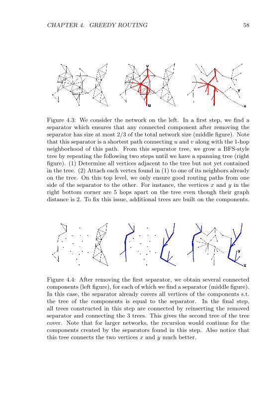
CHAPTER 4. GREEDY ROUTING 58
Figure 4.3: We consider the network on the left. In a first step, we find aseparator which ensures that any connected component after removing theseparator has size at most 2/3 of the total network size (middle figure). Notethat this separator is a shortest path connecting u and v along with the 1-hopneighborhood of this path. From this separator tree, we grow a BFS-styletree by repeating the following two steps until we have a spanning tree (rightfigure). (1) Determine all vertices adjacent to the tree but not yet containedin the tree. (2) Attach each vertex found in (1) to one of its neighbors alreadyon the tree. On this top level, we only ensure good routing paths from oneside of the separator to the other. For instance, the vertices x and y in theright bottom corner are 5 hops apart on the tree even though their graphdistance is 2. To fix this issue, additional trees are built on the components.
Figure 4.4: After removing the first separator, we obtain several connectedcomponents (left figure), for each of which we find a separator (middle figure).In this case, the separator already covers all vertices of the components s.t.the tree of the components is equal to the separator. In the final step,all trees constructed in this step are connected by reinserting the removedseparator and connecting the 3 trees. This gives the second tree of the treecover. Note that for larger networks, the recursion would continue for thecomponents created by the separators found in this step. Also notice thatthis tree connects the two vertices x and y much better.

CHAPTER 4. GREEDY ROUTING 59
Figure 4.5: Given the tree cover, each tree is embedded in a O(logn)-dimensional space. Note that each coordinate uses at most logn bits, re-sulting in coordinates of size O
`log2 n
´bits. In our example, 6 dimensions
per tree are enough.
Figure 4.6: Finally, the coordinates assigned for the trees are combinedto a single coordinate for each vertex. Using at most O(logn) trees, thesize of the coordinates is bounded by O
`log3 n
´bits. To send a message
from x to y, x compares the label of y to its neighbors n1 and n2 andforwards to the closer neighbor. The comparison is done tree by tree,e.g. for n1 we have L∞(10 7 7 2 8 1, 10 7 7 6 8 2) = 4 for the first tree andL∞(1 11 8 4 1 1, 0 12 9 3 2 1) = 1 for the second tree, giving an estimated dis-tance of 1 from n1 to y. Similarly, the estimated distance from n2 to y is 1as well. Therefore, x forwards the message to either of its neighbors.
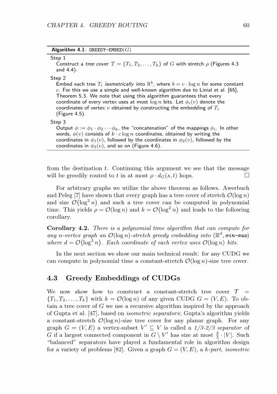
CHAPTER 4. GREEDY ROUTING 60
Algorithm 4.1: GREEDY-EMBED(G)
Step 1Construct a tree cover T = T1, T2, . . . , Tk of G with stretch ρ (Figures 4.3and 4.4).
Step 2Embed each tree Ti isometrically into Rb, where b = c · logn for some constantc. For this we use a simple and well-known algorithm due to Linial et al. [65],Theorem 5.3. We note that using this algorithm guarantees that everycoordinate of every vertex uses at most logn bits. Let φi(v) denote thecoordinates of vertex v obtained by constructing the embedding of Ti(Figure 4.5).
Step 3Output φ := φ1 · φ2 · · ·φk, the “concatenation” of the mappings φi. In otherwords, φ(v) consists of k · c logn coordinates, obtained by writing thecoordinates in φ1(v), followed by the coordinates in φ2(v), followed by thecoordinates in φ3(v), and so on (Figure 4.6).
from the destination t. Continuing this argument we see that the messagewill be greedily routed to t in at most ρ · dG(s, t) hops.
For arbitrary graphs we utilize the above theorem as follows. Awerbuchand Peleg [7] have shown that every graph has a tree cover of stretch O(logn)and size O
`log2 n
´and such a tree cover can be computed in polynomial
time. This yields ρ = O(logn) and k = O`log2 n
´and leads to the following
corollary.
Corollary 4.2. There is a polynomial time algorithm that can compute forany n-vertex graph an O(logn)-stretch greedy embedding into (Rd, min-max)where d = O
`log3 n
´. Each coordinate of each vertex uses O(logn) bits.
In the next section we show our main technical result: for any CUDG wecan compute in polynomial time a constant-stretch O(logn)-size tree cover.
4.3 Greedy Embeddings of CUDGs
We now show how to construct a constant-stretch tree cover T =T1, T2, . . . , Tk with k = O(logn) of any given CUDG G = (V,E). To ob-tain a tree cover of G we use a recursive algorithm inspired by the approachof Gupta et al. [47], based on isometric separators; Gupta’s algorithm yieldsa constant-stretch O(logn)-size tree cover for any planar graph. For anygraph G = (V,E) a vertex-subset V ′ ⊆ V is called a 1/3-2/3 separator ofG if a largest connected component in G \ V ′ has size at most 2
3· |V |. Such
“balanced” separators have played a fundamental role in algorithm designfor a variety of problems [82]. Given a graph G = (V,E), a k-part, isometric
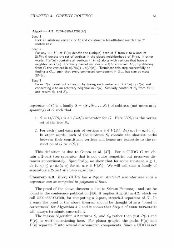
CHAPTER 4. GREEDY ROUTING 61
Algorithm 4.2: CUDG-SEPARATOR(G)
Step 1Pick an arbitrary vertex r of G and construct a breadth-first search tree Trooted at r.
Step 2For any u ∈ V , let P (u) denote the (unique) path in T from r to u and letN(P (u)) denote the set of vertices in the closed neighborhood of P (u). In otherwords, N(P (u)) contains all vertices in P (u) along with vertices that have aneighbor on P (u). For every pair of vertices u, v ∈ V construct Guv by deletingfrom G the vertices in N(P (u)) ∪ N(P (v)). Terminate this step successfully onfinding a Guv such that every connected component in Guv has size at most2|V |/3.
Step 3From P (u) construct a tree S1 by taking each vertex v in N(P (u)) \ P (u) andconnecting v to an arbitrary neighbor in P (u). Similarly construct S2 from P (v)and return S1 and S2.
separator of G is a family S = S1, S2, . . . , Sk of subtrees (not necessarilyspanning) of G such that
1. S = ∪iV (Si) is a 1/3-2/3 separator for G. Here V (Si) is the vertexset of the tree Si.
2. For each i and each pair of vertices u, v ∈ V (Si), dSi(u, v) = dG(u, v).In other words, each of the subtrees Si contain the shortest pathsbetween their constituent vertices and hence are isometric to the re-striction of G to V (Si).
This definition is due to Gupta et al. [47]. For a CUDG G we ob-tain a 2-part tree separator that is not quite isometric, but preserves dis-tances approximately. Specifically, we show that for some constant ρ ≥ 1,dSi(u, v) ≤ ρ · dG(u, v) for all u, v ∈ V (Si). We will call such a family ofseparators a 2-part stretch-ρ separator.
Theorem 4.3. Every CUDG has a 2-part, stretch-3 separator and such aseparator can be computed in polynomial time.
The proof of the above theorem is due to Sriram Pemmarju and can befound in the conference publication [40]. It implies Algorithm 4.2, which wecall CUDG-SEPARATOR, for computing a 2-part, stretch-3 separator of G. Ina sense the proof of the above theorem should be thought of as a “proof ofcorrectness” for Algorithm 4.2 and it shows that Step 2 of CUDG-SEPARATOR
will always terminate successfully.The reason Algorithm 4.2 returns S1 and S2 rather than just P (u) and
P (v), is worth mentioning here. For planar graphs, the paths P (u) andP (v) separate T into several disconnected components. Since a UDG is not
CHAPTER 4. GREEDY ROUTING 62
planar, it is possible to “hop” between the components by following edgesthat cross P (u) or P (v). However, UDGs have the nice property that if apair of edges cross then at least one pair of end points of the crossing edgesare neighbors. Therefore, if a path P is crossed by an edge u, v then eitheru or v is a neighbor of a vertex in P . Therefore, by removing Si, the pathPi along with its neighborhood, we ensure that the components are reallydisconnected and Si separates the given graph.
The tree cover of G can now be constructed by recursively applying al-gorithm CUDG-SEPARATOR for finding a 2-part, stretch-3 separator of G. Con-sider the trees S1 and S2 returned by the above algorithm. For each i = 1, 2,grow a BFS-style tree Ti from Si in the following way: Initially, set Ti = Si.While Ti is not spanning, repeat the following two actions: (1) Determinethe set of nodes N that are adjacent to Ti, but not yet on Ti. (2) For eachn ∈ N , connect n to an arbitrary neighbor on Ti \N .
T1 and T2 are the first two trees in the tree cover being constructed. Nowrecurse on the connected components in Guv. More specifically, supposethat the connected components in Guv are C1, C2, . . . , Ct and suppose thatfor each Ci we find Si1, Si2, a 2-part, stretch-3 separator and obtain thecorresponding trees T i1 , T i2. The collection T 1
1 , T21 , . . . , T
t1 is a forest and
we arbitrarily add vertices and edges to this forest to obtain a spanning treeof G. We similarly extend the forest T 1
2 , T22 , . . . , T
t2 to a spanning tree of
G, thus obtaining two more spanning trees for each level of the recursion.
Theorem 4.4. Given an n-vertex CUDG G, there is a polynomial-time algo-rithm that computes a constant-stretch tree cover T1, T2, . . . , Tk of G withk = O(logn). In addition, the stretch of the tree cover is upper-bounded by4.
Proof. The size of the tree cover is inO(logn) as the separator ensures a 1/3−2/3 cut such that each recursion step operates on a connected componentwhose size is reduced at least by a factor 2/3 compared to the previous step.A naive algorithm finds such a separator by testing each node pair u, v inStep 2 of Algorithm 4.2, requiring at most O
`n2´
tests for each level of therecursion. The test itself is trivial and can be done in O(n) operations. Theoverhead for the construction of corresponding BFS trees and the assemblyof the forests to a spanning tree is in O(n). Thus, the overall complexity forbuilding the tree cover is polynomial in n.
As for the stretch, consider an arbitrary non-neighboring pair s, t ofvertices in G. There are two cases depending on whether or not s and t areseparated by a separator Si constructed by Algorithm CUDG-SEPARATOR. Inthe following, we use the fact that Si is a shortest path Pi along with nodesin the neighborhood of Pi.

CHAPTER 4. GREEDY ROUTING 63
1. Vertices s and t are not separated in any level of the recursion. Inthis case s and t together lie on a separator S and we can show thatdS(s, t) ≤ 3 · dG(s, t). We need to analyze three cases: (a) If both, sand t lie on P , the connection along S is optimal (as P is a shortestpath). (b) Assume w.l.o.g. that only s lies on P and t is attached toan arbitrary neighbor y on P . Then, dP (s, y) ≤ dG(s, t) + 1, otherwiseP would not be a shortest path between s and y. (c) Similarly, if s andt are attached to x and y on P , respectively, dP (x, y) ≤ dG(s, t) + 2.As a result, dS(s, t) = dP (x, y) + 2 ≤ dG(s, t) + 4 ≤ 3 · dG(s, t) fornon-neighboring s and t.
2. Suppose that s and t are separated by a separator S1∪S2 in some levelof the recursion. Then, the shortest path between s and t intersectseither S1 or S2 in a point u. W.l.o.g. assume that it intersects S1.We now consider the tree T of the tree cover which was built from S1
and show that dT (s, t) ≤ 3 · dG(s, t) + 2 using an argument similar toTheorem 5.1 of Gupta et al. in [47]. Let s′ (t′) be the vertex on P1
closest to s (t) on the tree T . For our argument, we distinguish twocases: (a) if the optimal path from s to t passes through a point u on P1,we have that dT (s, s′) ≤ dG(s, u) and dT (t, t′) ≤ dG(t, u). In addition,dT (s′, t) ≤ dT (s, s′) + dG(s, t) + dG(t, t′). Combining the inequalities,we get that dT (s, t) = dT (s, s′) + dT (s′, t′) + dT (t′, t) ≤ 3 · dG(s, t).(b) If the optimal path between s and t does not pass through anyvertex of P1 (this is possible as we do not have a planar network), thenu is a node neighboring a node in P1. In that case, we can boundthe path to reach a first node in S1 by dT (s, s′) − 1 ≤ dG(s, u) anddT (t, t′) − 1 ≤ dG(t, u). dT (s′, t′) can be bounded as in the first case,and we obtain that dT (s, t) ≤ 3 · dG(s, t) + 2 ≤ 4 · dG(s, t) for non-neighboring s and t.
In both cases, there is a tree T along which the distance dT (s, t) is at most4 times longer than the optimal distance dG(s, t) on the graph G.
Theorem 4.5. There is a polynomial time algorithm that can compute forany n-vertex CUDG an O(1)-stretch greedy embedding into (Rd, min-max)where d = O
`log2 n
´. Overall, each coordinate uses O
`log3 n
´bits.
Proof. The claim follows directly from Theorem 4.1 and Theorem 4.4.
4.4 Simulation
Extensive simulations on large, randomly generated networks show that onaverage our embedding algorithms provide extremely low stretch routes, theaverage stretch being much smaller than the worst case guarantees proved

CHAPTER 4. GREEDY ROUTING 64
0
50
100
150
200
250
300
24
68
1012
1416
18201
1.05
1.1
1.15
1.2
Length of optimal pathAverage vertex degree
Ave
rage
str
etch
Figure 4.7: Average stretch as a function of the average vertex degree andthe length of the optimal path. Note that our greedy embedding guaranteesan upper bound on the stretch for any UDG. In practice, the stretch is alwaysbelow this bound and depends not only on the network topology, but also onthe length of the optimal route.
in the previous sections. We considered a range from very sparse to densenetworks for each of which we sampled random source and destination vertexpairs. The average routing overhead is around 10% and the worst stretch weever encountered is 3. Of course, such a simulation is much weaker than ourformal proof (Theorem 4.5) on the maximum stretch. However, it provides agood approximation for the average case and also helps to validate the overallapproach.
We used the sinalgo simulator described in Chapter 7 to construct thedesired network topologies which all live in an area of size 100 × 100 units.For each network, we deployed n vertices at random positions, constructedthe UDG with a transmission radius of 1 unit, and kept the giant connectedcomponent for the embedding. Varying n from 10,000 to 60,000 yields net-works in the desired density and size range. In the following, we characterizethe resulting networks by their average degree of the vertices, which growslinearly with n. With over 2,000 networks and 50,000 random source anddestination pairs, the simulation analyzed over 108 routing paths with anaverage length of 74 hops.
Figure 4.7 shows the average stretch as a function of the network density(the average degree of the vertices) and the length of the optimal path forwhich the samples were taken. It is interesting to note that the averagestretch partially depends on the length of the chosen route: close vertex pairstend to have at least one tree connecting them nearly optimally, yielding a
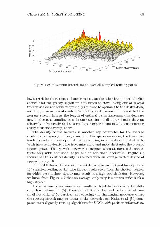
CHAPTER 4. GREEDY ROUTING 65
050
100150
200250
300
24 6 8 10 12
14 16 18 20
1
1.5
2
2.5
3
Length of optimal pathAverage vertex degree
Max
str
etch
Figure 4.8: Maximum stretch found over all sampled routing paths.
low stretch for short routes. Longer routes, on the other hand, have a higherchance that the greedy algorithm first needs to travel along one or severaltrees which do not connect optimally (or close to optimal) to the destination,resulting in an increased stretch. While Figure 4.7 seems to indicate that theaverage stretch falls as the length of optimal paths increases, this decreasemay be due to a sampling bias: in our experiments distant s-t pairs show uprelatively infrequently and as a result our experiments may be encounteringcostly situations rarely, as well.
The density of the network is another key parameter for the averagestretch of our greedy routing algorithm. For sparse networks, the tree covertends to include many optimal paths resulting in a nearly optimal stretch.With increasing density, the trees miss more and more shortcuts, the averagestretch grows. This growth, however, is stopped when an increased connec-tivity only adds additional edges but no additional shortcuts. Figure 4.7shows that this critical density is reached with an average vertex degree ofapproximately 10.
Figure 4.8 shows the maximum stretch we have encountered for any of the108 sampled routing paths. The highest peaks stem from the shortest routes,for which even a short detour may result in a high stretch factor. However,we know from Figure 4.7 that on average, only very few routes suffer such ahigh stretch.
A comparison of our simulation results with related work is rather diffi-cult. For instance in [52], Kleinberg illustrated his work with a set of verysmall networks of 50 vertices, not covering the challenging networks wherethe routing stretch may be linear in the network size. Kuhn et al. [59] com-pared several greedy routing algorithms for UDGs with position information.
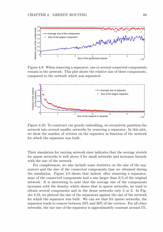
CHAPTER 4. GREEDY ROUTING 66
0 1 2 3 4 5 6
x 104
0
0.1
0.2
0.3
0.4
0.5
0.6
0.7
Size of the partitioned networkRel
ativ
e si
ze o
f the
com
pone
nts
Average size of the components
Size of the largest component
Figure 4.9: When removing a separator, one or several connected componentsremain in the network. This plot shows the relative size of these components,compared to the network which was separated.
0 1 2 3 4 5 6
x 104
0
0.2
0.4
0.6
0.8
1
Fra
ctio
n of
the
vert
ices
on
the
sepa
rato
r
Size of the network to separate
Average size of separator
Size of the largest separator
Figure 4.10: To construct our greedy embedding, we recursively partition thenetwork into several smaller networks by removing a separator. In this plot,we show the number of vertices on the separator in function of the networkfor which the separator was built.
Their simulation for varying network sizes indicates that the average stretchfor sparse networks is well above 3 for small networks and increases linearlywith the size of the network.
For completeness, we also include some statistics on the size of the sep-arators and the size of the connected components that we obtained duringthe simulation. Figure 4.9 shows that indeed, after removing a separator,none of the connected components had a size larger than 2/3 of the originalnetwork. It is interesting to note that the average size of the componentsincreases with the density, which shows that in sparse networks, we tend toobtain several components and in the dense networks only 2 or 3. In Fig-ure 4.10, we plotted the size of the separators against the size of the networkfor which the separator was built. We can see that for sparse networks, theseparator tends to remove between 10% and 30% of the vertices. For all othernetworks, the size size of the separator is approximately constant around 5%.

5Compact Routing with Any- and
Multicast
We finish this first thesis part on algorithm design with a routing scheme thatis slightly different from the previous routing techniques in that the nodesare allowed to store small routing tables. In return, the presented routingscheme not only supports unicast transmissions, but also offers efficient any-casting and multicasting. Thereby, we not only consider how fast a messageis delivered, but also how much overhead the algorithm generates. For in-stance, optimal routing is straightforward if each node stores in its routingtable the optimal path to every other node in the network. But this comesat a cost of O(n) routing entries, which easily exceeds the memory capacityof hardware limited network devices.
The multicasting feature may be extremely helpful to execute a queryonly on a subset of nodes. E.g. consider a fire detection system wherea coordinator first determines the set of nodes measuring a critical state.In subsequent rounds, it may only need to survey these nodes. Talking
u u
Figure 5.1: Support for efficient multicasting is crucial. If node u sendsa separate message to all destination nodes marked with solid circles (leftimage), it causes a much higher message overhead than if it utilizes an efficientmulticast algorithm (right image).

CHAPTER 5. COMPACT ROUTING WITH ANY- AND MULTICAST68
to each of them individually introduces a much higher message overheadthan efficiently multicasting a single message, see Figure 5.1. The gain ofmulticasting becomes even more substantial when the receiver set tends tobe clustered. In contrast to multicasting, anycasting becomes interestingwhen a node needs to send some data to any node of a given set. In theexample of the fire detection network, this may arise when a node measuringa critical state wants to inform one of several coordinators. The anycastingalgorithm picks the coordinator as to minimize transmission cost.
In addition to the routing tables, each node is assigned a special labelthat encodes routing information. This is similar to the greedy embeddingof Chapter 4 where we assigned a special set of coordinates to each node.But in contrast to the greedy embedding, we now talk about labels insteadof coordinates as the labels themselves cannot be used to deliver messages.Furthermore, remember that the size of the coordinates in the greedy embed-ding was in O
`log3 n
´bits for CUDGs and even in O
`log4 n
´bits for general
graphs. The labels used in this final routing scheme only require O(c · logn)bits for a small constant c that depends on the network topology. Thus, byadding a routing table on each node, we can drastically reduce the size of thelabels. But just as important as the size of the labels is the size of the rout-ing tables and the overhead of the message delivery. We will show that ourrouting tables are relatively small and prove our scheme to provide close tooptimal unicasting, and constant approximations to anycast and multicast.In addition, our assumption about the capabilities of the nodes is minimal:we only require that each node has a unique ID and that it can communicatewith its direct neighbors.
Unfortunately, the often studied UDG or UBG connectivity models arenot really appropriate for wireless networks because they do not considerperturbations of the wireless medium, e.g. caused by obstacles, and assumethe transmission radius to be perfectly circular. However, to ensure applica-bility of the proposed algorithms, the analysis should be on a connectivitymodel that characterizes wireless networks as accurately as possible. Clearly,any network connectivity can be described using a general graph. But takinginto account the limited range of wireless devices, we observe that nodes aremostly connected with other nodes in their proximity, which results in a farmore regular connectivity graph than a general graph. Although close-bynodes may be out of communication range due to obstacles, a node is typi-cally highly connected to nodes in its surroundings. In other words, even inenvironments with many obstacles, the total number of mutually indepen-dent1 neighbors of a node is likely to be small [84].
We exploit the slightly more general formulation of this property thattakes into account the multi-hop nature of the network: Given a h-hop neigh-borhood of a node v, it is possible to cover all these nodes with only a small
1Two nodes are independent if they are not (direct) neighbors.

CHAPTER 5. COMPACT ROUTING WITH ANY- AND MULTICAST69
number of h2
-hop neighborhoods. Similar to before, this property states thatin any h-hop neighborhood, one can pick only a relatively small subset ofnodes with pairwise distance larger than h
2. Figure 5.2 shows the deployment
of 39 sensor nodes in our office building and how the nodes are connected[31]. In this network, the 2-hop neighborhood of any node can be covered byat most five 1-hop neighborhoods. The figure shows the 2-hop neighborhoodof node v, which is covered by four 1-hop neighborhoods.
These observations motivate to characterize the network connectivity byA, the maximum number of half-sized neighborhoods that are necessary tocover any given neighborhood. This number is expected to be quite smallfor most wireless networks, e.g. a small two-digit number. Being the onlyparameter to describe the network, we can adjust A to apply our analysis tovirtually any wireless network topology, including obstacle-rich deploymentsin 3D and worst case scenarios. Furthermore, because the presented routingalgorithms are self-adaptive and need not to know the value of A, they aregood for any network. It is only the performance of the routing algorithmsthat depends on the value of A.
In the sequel we describe the network connectivity by a weighted graphG = (V,E) where each network node is mapped to a node of the graph, and aweighted edge is present between any two nodes within mutual transmissionrange. We observe that the coverability property described above matchesthe definition of a constant doubling metric2 on G (see Definition 5.2). Thedistance metric M associated with G corresponds to the metrization of Gusing the cost-function dM(a, b) which assigns to each pair (a, b) ∈ V ×V thecost of the least cost path between a and b. Our analysis holds for a moregeneral class of networks, where each link may be assigned a cost, e.g. thenumber of retransmissions needed to send a message over the link. Settingall link costs to 1, we obtain the hop-metric discussed above.
Definition 5.1 (Ball). Given a node v ∈ V , the ball Bv(r) with radius r de-notes the set of nodes with distance at most r from v: Bv(r) = u|dM(v, u) ≤r.
Definition 5.2 (Constant Doubling Metric). A graph G = (V,E) fulfillsthe doubling metric property if any ball Bv(r) can be covered 3 by a constantnumber of balls B( r
2) with half the radius: For r ≥ 0 and ∀v ∈ V : ∃U ⊆ Bv(r)
such that |U | = O(1) and Bv(r) ⊆Su∈U Bu( r
2). If |U | is bounded by 2α for a
constant α, we say that the metric associated with G has doubling dimensionα.
We point out that the value of α = dlog2Ae is quite small for mostwireless networks, e.g. around 3 or 4.
2A metric assigns to each node-pair (a, b) ∈ V × V a cost satisfying non-negativity,identity of indiscernibles, symmetry and triangle inequality.
3A ball B is covered by a set of balls b1, . . . , bn if ∀u ∈ B : ∃i such that u ∈ bi.

CHAPTER 5. COMPACT ROUTING WITH ANY- AND MULTICAST70
v
Figure 5.2: The figure shows a deployment of 39 nodes in an office buildingand how they are connected. The nodes in black denote a 2-hop neighborhoodof node v. These nodes can be covered by four 1-hop neighborhoods indicatedwith the dashed lines and rooted at the nodes with the small white dot.
5.1 Related Work
One milestone in the area of compact routing schemes was laid by Pelegand Upfal in [76], where they examine the trade-off between the efficiencyof a routing algorithm and its space requirements. They present a stretch-krouting algorithm for general graphs with an average routing table size of
O“k3n1/k logn
”bits and O(logn) bit labels. The renaming (labeling) of the
network nodes is a widely used technique to reduce the routing table size.In fact, any routing algorithm that does not rename the nodes and requiresa stretch below 3 may need routing tables of Ω(n) bits [42]. For constantdoubling metrics, we know that the stretch is above 9−ε if the routing tables
size is o“n(ε/60)2
”[53].
In his recent work [91], Talwar described a (1 + ε) stretch routing schemefor α-doubling metrics with routing tables of O(1/(εα))α log2+α Θ bits andlabel-size O(α log Θ) bits where Θ is the diameter of the network. This workwas improved by Chan et al. in [19] by reducing the storage overhead to(α/ε)O(α)(log Θ)(log ∆) bits per node and a label size of O
`α log (ε−1)
´log Θ
bits, with ∆ denoting the maximal degree of any node.Slivkins presented two improved compact routing schemes in
[88]. The first uses (ε)−O(α)(log Θ)(log ∆) bits per routing ta-ble and O
`α log (ε−1)
´log Θ bits per label, whereas the second
scheme uses ε−O(α)(log Θ)(log log Θ)(logn) routing table bits and2O(α)(logn) log (ε−1 log Θ) bits for each label.
In their seminal work [3], Abraham et al. presented the first

CHAPTER 5. COMPACT ROUTING WITH ANY- AND MULTICAST71
compact routing scheme with dlogne bit labels and routing tables ofε−O(α) logn log (min (Θ, n)) bits. This work emphasized on scale-freedom,i.e. independence of Θ. Dropping this constraint, their technique easilyyields O(Θ) bit labels. In addition, the authors provide a scale-free name-independent routing scheme, including the matching lower bounds.
Our work does not quite achieve the bounds of [3], our routing ta-bles are of size O
`1ε
´α(log Θ)(O(α) + log ∆) and the routing labels require
2αdlog Θe+dlogne bits4. This small overhead allows us to build an all-in-onerouting scheme that not only supports unicasting (Chapter 5.4), but also pro-vides constant approximations to anycasting (Chapter 5.6) and multicasting(Chapter 5.5). Furthermore, we present a distributed algorithm to constructthe labeling and routing tables in Chapter 5.7.
5.2 Definitions and Preliminaries
We first define some further terms and state properties of doubling metricsthat will turn out to be handy. We start with the definition of a ρ−net,which is closely related to maximal independent sets and dominating sets.
Definition 5.3 (ρ−net). A subset U of the node-set V of a graph G = (V,E)is a ρ−net if each node in V has distance at most ρ to at least one node inU , and the mutual distance between any two nodes in U is strictly larger thanρ. Formally, a set U ⊆ V is a ρ−net of G = (V,E) if
∀v ∈ V : ∃u ∈ U : dM(v, u) ≤ ρ and∀u1, u2 ∈ U : dM(u1, u2) > ρ.
We say that a node u ∈ ρ−net covers the nodes contained in Bu(ρ). Thus,each node of the network is covered by at least one u ∈ ρ−net. In the sequel,we denote the nodes of a ρ−net as net-centers of the ρ−net.
Given a constant doubling metric, we know that for every ball Bv(r), it ispossible to cover all nodes in Bv(r) with 2α balls of half the radius. However,this is only a feasibility statement and does not give an upper bound on thenumber of B( r
2) that may be deployed to cover Bv(r). The following property
gives an upper bound on the number net-centers of r2−net a ball Bv(r) may
cover.
Property 5.4 (Sparseness). For x ∈ N0, each ball Bv(2xρ) covers at most2(1+x)α nodes from an arbitrary ρ−net on the same graph with constant dou-bling dimension α.
Proof. By recursively applying the definition of the doubling metric, we ob-serve that it is possible to cover Bv(2xρ) with at most 2(1+x)α balls of radiusρ2. Assume we know such a covering C with |C| ≤ 2(1+x)α.
4Note that even for a huge network of 106 nodes, diameter 104, and α = 4, the routinglabels are still below the size of an IPv6 address and fit in the tiny messages of today’ssensor nodes.
CHAPTER 5. COMPACT ROUTING WITH ANY- AND MULTICAST72
In order to see that Bv(2xρ) covers at most 2(1+x)α net-centers U =u1, u2, ..., u|U| from any ρ−net, we first observe that the distance betweenany two distinct nodes in U exceeds ρ. Secondly, by the definition of a cover,each uj ∈ U is covered by at least one ball from the cover C. Because theballs in C have radius ρ
2and the distance between any two uj is more than
ρ, any c ∈ C covers at most one uj ∈ U . Thus, |U | ≤ |C| ≤ 2(1+x)α, whichcompletes the proof.
Along with this upper bound on the number of net-centers covered by aball, we can give an upper bound on the number of net-centers of a givenρ−net that may cover any given node v. In particular, we are interested inthe maximum number of net-centers of a ρ−net that cover a node v, if eachnet-center u covers an extended ball Bu(2xρ).
Property 5.5 (Dominance). Given a ρ−net on a α-doubling metric repre-sented by the graph G = (V,E) where each net-center u covers Bu(2xρ) withx ∈ N0, then any node v ∈ V is covered by at most 2(x+1)α net-centers fromthe ρ−net.
Proof. If v is covered by a net-center u, then u is at most 2xρ away fromv. Therefore, it is sufficient to show that Bv(2xρ) contains at most 2(x+1)α
ρ−net-centers, which follows from Property 5.4.
Corollary 5.6 (Dominance II). Given a ρ−net on a α-doubling metric rep-resented by the graph G = (V,E) where each net-center u covers Bu(iρ) withi ∈ R+, i > 1, then any node v ∈ V is covered by at most 22αiα net-centersfrom the ρ−net.
5.3 Dominance Net
Due to our minimal assumptions about the nodes’ capabilities (unique IDand communication with direct neighbors), our routing algorithms need somemeans to characterize the network.
We propose to obtain this information through a dominance net, which isa hierarchic locality-preserving decomposition of the network. In a nutshell,the dominance net is built of several layers of ρ−nets with exponentiallyincreasing radius ρ, each of which covers the entire network. In the sequel,we will show how to build a dominance net with the following properties:
1. The number of layers is at most 1 + dlog Θe, where Θ is the diameterof the network.5
2. Each node is dominated by at most O(log Θ) nodes.
5Throughout this chapter, log stands for the binary logarithm.
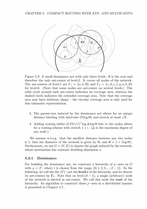
CHAPTER 5. COMPACT ROUTING WITH ANY- AND MULTICAST73
v
R
ab
c
de
fg
Figure 5.3: A small dominance net with only three levels. R is the root andtherefore the only net-center of level-2. It covers all nodes of the network.The net-centers of level-1 are Γ1 = a, b, R and Γ0 = c, d, e, f, g, a, b, Rfor level-0. (Note that some nodes are net-center on several levels.) Thesolid circle around each net-center indicates its coverage area, whereas thedashed circle indicates the extended coverage area. Note that the coveragearea may have arbitrary shape – the circular coverage area is only used forthis schematic representation.
3. The parent-tree induced by the dominance net allows for an uniquedistance labeling with label-size O(log Θ) and stretch at most
√6.
4. Adding routing tables of O(1/ε)α log ∆ log Θ bits to the nodes allowsfor a routing scheme with stretch 1 + ε. (∆ is the maximum degree ofany node.)
We assume w.l.o.g. that the smallest distance between any two nodesis 1, that the diameter of the network is given by Θ, and ϑ = 1 + dlog Θe.Furthermore, we use G = (V,E) to denote the graph induced by the network,whose metrization has constant doubling dimension α.
5.3.1 Dominance
For building the dominance net, we construct a hierarchy of ρ−nets on Gwith ρ = 2i, where i is chosen from the range 0, 1, 2, 3, ..., ϑ − 1. In thefollowing, we call the the (2i)−net the level-i of the hierarchy, and we denoteits net-centers by Γi. Note that on level-(ϑ − 1), a single (arbitrary) nodeof the network is elected as net-center. We call this node the root of thehierarchy. An algorithm to construct these ρ−nets in a distributed manneris presented in Chapter 5.7.

CHAPTER 5. COMPACT ROUTING WITH ANY- AND MULTICAST74
R
1s
1p
2p
2s3p
21
1
2
R2
3
1
Figure 5.4: The left picture shows the dominance-tree corresponding to thedominance-net of Figure 5.3. The tree on the right is the cover-tree ofnode v, a tree-representation of v’s label. At depth i, this tree containsthe enumeration-values of the net-centers of level-(ϑ− i− 1) which cover v.The letter p indicates a primary net-center, s a secondary net-center.
We define the dominance on this ρ−net hierarchy in the following way:A net-center γi ∈ Γi is dominated by a net-center γ ∈ Γi+1 iff γi ∈ Bγ(2i+1).Thus, each net-center (except the root) is dominated by at least one net-center of the next higher level.
5.3.2 Naming Scheme
Given the dominance-net, we name the net-centers in the following way: Eachnet-center v except for the root node selects exactly one6 of its dominators tobe its parent P(v). This results in a dominance-tree with depth ϑ−1. Eachparent enumerates its children and informs each of them about the assignedenumeration value. The naming scheme is defined recursively: The root hasan empty name, while any other net-center obtains its name by appendingits enumeration value to its parents name.
Figure 5.3 shows a sample dominance net with only three levels. Theleft picture of Figure 5.4 shows the corresponding dominance-tree with theassigned enumeration values. The name of a net-center is obtained by walkingfrom the corresponding node of the dominance-tree towards the root andconcatenating the enumeration values of the visited nodes. E.g. the nameof net-center g is R:1:2 whereas the name of c is R:2:3. The uniquenessof the names is guaranteed due to the tree structure, where each net-centeris identified through its parent and the enumeration value assigned by theparent.
Because any net-center may be parent of at most 22α net-centers (Prop-erty 5.4), the enumeration values can be represented with at most 2α bits.Thus, the name may grow by 2α bits on each level, which results in a maxi-mum name size of 2αdlog Θe = O(log Θ) bits for net-centers on level-0.
6For performance reasons, each net-center may choose the closest net-center of thenext higher level.

CHAPTER 5. COMPACT ROUTING WITH ANY- AND MULTICAST75
5.3.3 Dominance Labeling
Based on the dominance-net and the corresponding naming scheme, eachnode v of the graph G assigns itself a label L(v) of size O(log Θ) whichallows for efficient routing, multicasting, anycasting, and distance labeling.In the remainder of this section, we show the following theorem:
Theorem 5.7 (Compact Labels). The nodes of G can be assigned uniquelabels of size O(log Θ) allowing approximate distance queries of stretch
√6
between any two nodes.
We use an extended dominance net for the labeling, where a net-centerγ ∈ Γi covers all nodes in Bγ(2i+1), cf. Figure 5.3. This extension results inan overlap of the net-covers, which allows to rule out borderline effects wheretwo close-by neighbors are not covered by common net-centers. Given thisextended dominance set, each node v determines the net-centers by whichit is covered. Essentially, the label of v contains the name of all net-centersthat cover v.
In order to obtain the desired label size for a node v, we cannot simplystore all names of the covering net-centers: By construction, there are at mostϑ levels, each of which has at most 22α net-centers covering v (Property 5.5).From the previous section, we know that the naming for the net-centers usesat most 2α(ϑ− i−1) bits on level-i, which bounds the maximum label lengthtoPϑi=0 22α2α(ϑ− i− 1) = O
`ϑ2´
= O`log2 Θ
´. To receive the O(log Θ)
label size, we make use of the following lemma which shows that only partialnet-center names need to be stored for each covering net-center.
Lemma 5.8 (Parental Cover). If a net-center c ∈ Γi covers a node v in theextended dominance net, then its parent P(c) ∈ Γi+1 covers v as well.
Proof. The net-center c on level-i only covers nodes in Bc(2i+1) in the ex-tended dominance net. Therefore, dM(v, c) ≤ 2i+1. Because the par-ent P(c) of c is chosen from the ordinary7 dominance net and P(c) ∈Γi+1, dM(c,P(c)) ≤ 2i+1. Using the triangle inequality we receive thatdM(v,P(c)) ≤ dM(v, c) + dM(c,P(c)) ≤ 2i+2. The claim follows becauseP(c) covers BP(c)(2
i+2) in the extended dominance net, which includes v.
5.3.4 Cover Tree
The label L(v) of a node v is the flat representation of a cover tree thatefficiently describes all net-centers that cover v. This tree is rooted at theroot node. The body of the cover tree is defined recursively: At depth i, thetree contains the net-centers γ ∈ Γϑ−i−1 that cover v. Each γ in the covertree is connected to its parent P(γ). This is possible because we know from
7Ordinary means not in the extended dominance net.
CHAPTER 5. COMPACT ROUTING WITH ANY- AND MULTICAST76
Lemma 5.8 that if γ covers v, then also P(γ) covers v and therefore must bepresent in the cover tree.
Because the name of a net-center is defined as the recursive concate-nation of the enumeration values of its parents in the dominance net (seeChapter 5.3.2) and the same parenthood persists in the cover tree, each nodeof the cover tree only needs to store the enumeration value of its correspond-ing net-center. The name of a net-center c in the cover tree can be obtainedby prefixing the enumeration value of c with the name of P(c), which is ob-tained recursively. Therefore, each node of the cover tree carries at most 2αbits, see Figure 5.4 for an example. We also know from Property 5.5 thatthere are at most 22α net-centers per level covering node v. Because thedepth of the tree is at most ϑ − 1, we deduce that the cover tree holds atmost α22α+1ϑ bits. The serialization of the cover tree to a flat data structureis straightforward and can be done introducing only two additional bits pernet-center, which leads to a label size of (2α+ 2)22αϑ ∈ O(log Θ) bits.
In the remainder of this discussion, we rely on a slightly enhanced nodelabeling where each node v not only stores the net-centers by which it iscovered, but also indicates their type. We distinguish two types of net-centersdepending on their distance to v: A net-center c ∈ Γi is called primary ifv ∈ Bc(2i). Otherwise, the net-center is called secondary, i.e. a secondarynet-center covers v only in the extended dominance net, whereas a primarynet-center covers v already in the ordinary dominance net. This additionalbit per net-center does not significantly increase the size of the cover tree,which becomes at most (2α + 3)22αϑ = O(log Θ) bits. This proves the firstpart of Theorem 5.7.
5.3.5 Distance Approximation
To obtain the distance between two nodes a and b given their labels L(a)and L(b), we determine the smallest level-i for which a and b have at leastone common net-center. Let ρ = 2i be the ordinary coverage radius of level-iand C ⊆ Γi the set of common net-centers on level-i.
We immediately get a lower bound on the distance between a and b byobserving that if dM(a, b) ≤ ρ/2, there exists a net-center c ∈ Γi−1 thatcovers both a and b. Therefore, dM(a, b) > ρ/2. For the remainder of thisproof, we need to consider the following three cases only:
1. If there is a net-center c ∈ C s.t. c is primary for both a and b,then dM(a, b) ≤ 2ρ and therefore dM(a, b) ∈ (ρ/2, 2ρ]. This prop-erty holds due to the triangle inequality: Because a and b are pri-mary, dM(a, c) ≤ ρ and dM(b, c) ≤ ρ, which implies that dM(a, b) ≤dM(a, c) + dM(c, b) ≤ 2ρ.
2. If all net-centers c ∈ C are secondary for a and b, dM(a, b) ∈ (ρ, 4ρ].Again, the upper bound is given by the triangle inequality: dM(a, c) ≤

CHAPTER 5. COMPACT ROUTING WITH ANY- AND MULTICAST77
2ρ and dM(b, c) ≤ 2ρ, and therefore dM(a, b) ≤ 4ρ. The lower boundstems from the fact that any primary net-center of a would cover b ifdM(a, b) ≤ ρ, and vice versa.
3. Finally, if there is at least one net-center c ∈ C s.t. c is primary foreither a xor b, then dM(a, b) ∈ (ρ/2, 3ρ]. W.l.o.g. assume that c isprimary for node a. Then dM(a, c) ≤ ρ and dM(c, b) ≤ 2ρ. Therefore,dM(a, b) ≤ dM(a, c) + dM(c, b) ≤ 3ρ.Note: If for either a xor b there is no c ∈ C s.t. c is primary for thenode, then dM(a, b) ∈ (ρ, 3ρ]. The increase in the lower bound holdsbecause no primary net-center of a xor b covers the other node, whichis only possible if dM(a, b) > ρ.
Given the interval (r1, r2] for the possible values of dM(a, b), we setdM(a, b) =
√r1r2, the geometric mean of the two bounds. The maximum
factor by which the approximation is off from the actual distance ispr2/r1.
Therefore, our labeling scheme suffers from a maximum stretch in the thirdcase, which is at most
√6. This concludes the proof of Theorem 5.7.
5.4 Routing
We present a single destination routing algorithm (SDR) which will be usedas a building block for multicasting and anycasting. In SDR, a message needsto be forwarded from a sender node s to a single target node t. The stretchSA of a routing algorithm A is defined as SA = maxs,t∈V
dA(s,t)dM(s,t)
where
dA(s, t) is the length of the path found by the routing algorithm. Clearly,we desire the stretch to be as small as possible, but this comes at a certaincost. In our approach, the stretch is coupled with the routing table size,i.e. lowering the stretch induces bigger routing tables. Our unicast routingresult is summarized in the following theorem, where Θ is the diameter ofthe network, and ∆ stands for the maximum degree of a node.
Theorem 5.9. For a fixed ε with 0 < ε ≤ 2, SDR routes messages withstretch (1 + ε) such that the chosen path by SDR is at most (1 + ε)dM(s, t).The header size of each message is at most 2αdlog Θe+ dlogne bits, and therouting tables stored at each node require only O
`1ε
´α(log Θ)(O(α) + log ∆)
bits.
The routing scheme is based on the node labeling introduced in Chap-ter 5.3.4 and is quite simple: The sender node s extracts from L(t) the nameN of an arbitrary primary net-center γ ∈ Γ0 that covers the target node t.This name N and the ID of t serve as header information in the message,which uses at most 2αdlog Θe+ dlogne bits (see Chapter 5.3.2). Rememberthat N is a concatenation of the enumeration values of γ and its ancestors

CHAPTER 5. COMPACT ROUTING WITH ANY- AND MULTICAST78
in the dominance tree. Therefore, N encodes the names of exactly one net-center (primary or secondary) per level that covers t (Lemma 5.8). Let usdenote these net-centers by c0, c1, c2, c3, . . . , 2ϑ−2, where ci is the net-centeron level-i. The forwarding mechanism works as follows: Each node that re-ceives a message finds the net-center ci on the lowest level for which it hasrouting information and forwards the message in this direction. This is re-peated until the message hits a direct neighbor of t which sends the messagedirectly to t based on its neighborhood list.
In order to support this forwarding scheme, each node needs to store howto reach some of the net-centers in its surroundings. For this purpose, eachnet-center γ ∈ Γi advertises itself to Bγ(η2i) with η = 8
ε+ 6. I.e. every
node in this ball stores how to reach γ on an optimal path. In fact, it sufficesto store the neighbor node lying on the optimal path. This correspondsto the shortest path problem (in a restricted area) and can be obtained bydistributed versions of the Dijkstra algorithm. Thus, the routing table of eachnode v stores how to reach any net-center γ ∈ Γi iff dM(v, γ) ≤ η2i. Thiscan be seen as a mapping from the name of the net-center γ to the neighborof v which lies on the shortest path to γ. Before we show in Chapter 5.4.2that the routing information can be stored efficiently, we prove that SDRfinds good routing paths.
5.4.1 (1 + ε)-Stretch Routing
We first observe that once the message has reached a net-center covering t,it can be forwarded to a net-center covering t on a lower level:
Lemma 5.10 (Net-Center Hopping). Given a net-center ci ∈ Γi that coversthe destination node t, the routing table of ci contains entries for all net-centers ci−x ∈ Γi−x covering t. This holds for x ≤ blog2
η−22c.
Proof. Suppose that cj ∈ Γj with j < i is a net-center of t. Due to therouting table construction, all nodes in Bcj (η2j) have routing table entriesto cj . Using the triangle inequality, we know that dM
`cj , ci
´≤ 2j+1 + 2i+1.
Therefore, ci is sure to have a routing table entry if dM`cj , ci
´≤ η2j , which
holds if x = i− j ≤ blog2η−2
2c.
The following proof of the routing stretch describes the worst case scenariowhere the message visits the net-centers ci, ci−x, ci−2x, . . . , where ci isthe net-center towards which s forwards the message, cf. Figure 5.5.
Proof. (Routing Stretch) Let ci be the net-center on the lowest level for whichs has routing information. Following the routing algorithm, the message isfirst forwarded to ci, from where it can be forwarded to ci−x with x =blog2
η−22c (Lemma 5.10). This step is repeated until the message reaches

CHAPTER 5. COMPACT ROUTING WITH ANY- AND MULTICAST79
s tdM(s, t)
ci
ci−x
ci−2x
Figure 5.5: Schematic illustration (out of scale) of the worst case scenariowhere a message to be sent from s to t first visits ci, then ci−x and so on, untilit reaches a level-0 net-center covering t which directly delivers the message.
a net-center on level-0, which directly delivers the message. Thus, the totaldistance dSDR(s, t) of SDR is bounded by
dM“s, ci
”+ dM
“ci, ci−x
”+ dM
“ci−x, ci−2x
”+ · · ·+ 1
Using the triangle inequality, we obtain that dM`s, ci
´≤ dM(s, t)+2i+1 and
for j ≥ 0 : dM“ci−jx, ci−(j+1)x
”≤ 2 · 2i−jx + 2 · 2i−(j+1)x. Therefore,
dSDR(s, t) ≤ dM(s, t) + 4
∞Xj=0
2i−jx (5.1)
= dM(s, t) + 4
∞Xj=0
2i
2blog2η−22 cj
(5.2)
≤ dM(s, t) + 2i+2∞Xj=0
„4
η − 2
«j(5.3)
≤ dM(s, t) + 2i+2 η − 2
η − 6(5.4)
We obtain (3) from (2) by observing that 2blog2η−22 cj ≥ 2j log2
η−24 =
((η − 2)/4)j . To obtain (4), note that the sum in (3) sums the elements of ageometric series with factor 4
η−2= ε
2+ε< 1.
Because s does not have a routing table entry for cj with j < i, we deducethat dM(s, t) > (η − 2)2i−1. This holds because dM
`ci−1, t
´≤ 2 · 2i−1 and
ci−1 advertises itself to Bci−1(η2i−1). Therefore, s has a routing entry toci−1 if dM(s, t) ≤ (η − 2)2i−1.
Putting together the two results, we obtain that the routing stretch ofSDR is

CHAPTER 5. COMPACT ROUTING WITH ANY- AND MULTICAST80
SSDR ≤ dSDR(s, t)
dM(s, t)≤ 1 +
2i+2 η−2η−6
2i−1(η − 2)
= 1 +8
η − 6= 1 + ε.
This constitutes the proof for the routing stretch statement in Theo-rem 5.9.
Throughout the proof, we assumed that the message visits the net-centersci, ci−x, ci−2x, . . . , which is the worst case scenario. A considerable per-formance boost can be achieved in the average case if the routing algorithmtests in each step for a closer net-center. The key idea is that while themessage is being routed towards cj , it tests after each hop whether the cur-rent node can route towards a closer net-center ck with k < j. If this is thecase, the message immediately routes towards ck. This produces a shortcuttowards t, reducing the routing path and therefore the stretch.
5.4.2 Compact Tables
The construction of the routing table is similar to the cover tree presentedin Chapter 5.3.4 with the main difference that each net-center γ ∈ Γi coversan area which depends on ε, namely Bγ(( 8
ε+ 6)2i). Because of this mutable
coverage radius, we need to restate Lemma 5.8:
Lemma 5.11 (Parental Cover II). If a node v has routing information aboutnet-center γ ∈ Γi, then v also has a routing entry to P(γ) unless γ is theroot node.
Proof. Node v has routing information about γ ∈ Γi iff v ∈ Bγ(η2i) withη = 8
ε+ 6. Because dM(γ,P(γ)) ≤ 2i+1 and dM(γ, v) ≤ η2i, dM(v,P(γ)) ≤
(η+ 2)2i using the triangle inequality. Therefore, it is sufficient to show that(η + 2)2i ≤ η2i+1 such that v ∈ BP(γ)(η2i+1). The inequality holds becauseη = 8
ε+ 6 ≥ 2.
Using the same arguments as in Chapter 5.3.4, we can show that all net-centers for which a node v needs to store routing information can be be storedin a tree, where each tree node corresponds to one net-center. Each node ofthe tree only holds the enumeration value of the corresponding net-center γand the routing information on how to reach γ. Recall that the enumerationvalue fits in 2α bits and the routing information is the neighbor node whichlies on the optimal path between v and the corresponding net-center. Thus,the routing information uses at most log ∆ bits, where ∆ is the maximumdegree of a node.

CHAPTER 5. COMPACT ROUTING WITH ANY- AND MULTICAST81
Each node v needs to keep routing information for at most 22α`
8ε
+ 6´α
net-centers per level (Corollary 5.6). Because there are at most ϑ levels, thetree has at most 22α
`8ε
+ 6´αϑ nodes, each of which needs to store 2α+log2 ∆
bits. We have already noted that such a tree can be stored in a flat datastructure adding only two bits per node, which results in a total routing tablesize of (2α+ log2 ∆ + 2)22α
`8ε
+ 6´αϑ = O
`1ε
´α(log Θ)(O(α) + log ∆) bits.
This concludes the proof of Theorem 5.9.
5.5 Multicasting
We now have developed all tools that allow for efficient multicasting from asender node s to a set U of receivers. In a nutshell, the sender s approximatesa minimum spanning tree (MST) on the set s∪U using Kruskal’s algorithmand then routes the message along this tree towards all receivers. Note thatin contrast to the centralized multicasting presented in [95], our approach isdistributed. We show the following result:
Theorem 5.12. Consider a network G = (V,E) on which a dominance netwith the associated labeling and routing tables was created. Then, any sendernode s ∈ V can multicast messages to any set U ⊂ V with constant stretch.The cost associated with the multicasting is at most 12(1+ε) times the cost ofan optimal multicasting algorithm, which knows the entire network topology.
Proof. We need to show that the path along the MST approximation is atmost 12(1 + ε) longer than the optimal path, which is given by a minimumSteiner tree (MStT) on the set s ∪ U and the remaining nodes as Steinerpoints. The stretch is composed of three parts: First, a MST on s ∪ U is a2-approximation of the corresponding MStT. This result was shown by Kouet al. in [54]. The (1+ ε) part is caused by the SDR routing scheme, which isresponsible to forward the message along the tree. Lastly, the construction ofthe MST is based on the stretch-
√6 distance labeling. As a result, Kruskal’s
algorithm may not choose the shortest, but up to a factor 6 longer edges ineach step, which results in a MST approximation at most 6 times longer thanthe MST.
5.6 Anycast
As for the special case of anycasting, where a message has to be routedto exactly one node of a given node set U , we provide a constant stretchalgorithm to deliver the message:
Theorem 5.13. The node labeling from Chapter 5.3.4 and SDR from Chap-ter 5.4 allow for a 6(1 + ε)-approximation to anycast.

CHAPTER 5. COMPACT ROUTING WITH ANY- AND MULTICAST82
Proof. Based on the distance labeling, pick the node u ∈ U which seemsclosest to the sender node s and send the message to u. Because of thestretch of the distance labeling, this approach may pick a receiver that is upto 6 times further away from s than the optimal receiver. The (1 + ε) factorstems from the SDR routing scheme.
5.7 Distributed Dominance Net Construction
In this last section, we describe an efficient distributed algorithm to buildthe ρ−nets that constitute the dominance net. Recall from Chapter 5.3.1that the dominance net consists of ϑ ρ−nets with exponentially increasing ρchosen from 1, 2, 4, ..., 2ϑ−1.
To start, we would like to point out that a centralized algorithm to builda ρ−net on G = (V,E) is straightforward: Greedily pick an arbitrary v ∈ V ,add v to Γ and remove all nodes in Bv(ρ) from V . Repeat until V is theempty set. By construction, the distance between any two net-centers islonger than ρ and each node v ∈ V is covered by at least one net-center.
For our distributed algorithm, we exploit the fact that a ρ−net is a max-imal independent set (MIS) for the ρ metric closure8 Gρ = (V,Eρ). Thisimmediately leads to a simple distributed algorithm to create a ρ−net: cre-ate a ρ metric closure where each node v ∈ V has all nodes in Bv(ρ) asdirect neighbors. Then, run a distributed MIS algorithm on the closure andpick the nodes in the MIS to be the net-centers of the ρ−net. There existsa broad assortment of distributed MIS algorithms, e.g. there is an elegantrandomized algorithm with expected running time in O(logn) by Luby [69].More recently, Kuhn et al. [57] described a deterministic MIS constructionfor bounded independence graphs with running time O(log ∆ log∗ n).
The above algorithm is realistic for small values of ρ. However, whenρ approaches Θ, the nodes tend to have huge neighborhoods, consisting ofnearly all other nodes of the network. This may quickly exceed the memorycapabilities of simple network nodes, especially when considering large net-works. To overcome this issue, we present not only a relatively fast, but alsomemory conservative algorithm to construct the ρ−net hierarchy.
5.7.1 Sequential ρ−nets
Algorithm 5.1 describes in high-level pseudocode the steps each node v ofthe network performs in order to create the dominance nets. At the end ofthe algorithm, each node knows for which ρ−nets it is a net-center, and italready holds the complete routing table for the SDR routing scheme pre-sented in Chapter 5.4. In a nutshell, the algorithm is recursive and performsthe following two steps to build the ρ−net of level-i.
8The n metric closure of a graph G = (V,E) is the graph Gn = (V,En) withEn = (u, v)|u, v ∈ V ∧ u 6= v ∧ dM(u, v) ≤ n

CHAPTER 5. COMPACT ROUTING WITH ANY- AND MULTICAST83
Algorithm 5.1: Dominance Net (Code for node v)
state = active1
Main()2
N = nodes in Bv(1)3
Build MIS with neighbor set N4
if v /∈ MIS then5
state = passive6
else7
Inform Bv(1) v is a net-center of level-08
Add routing entries to v in Bv(η) η = 4ε + 39
JoinMIS(1)10
end11
JoinMIS(i)12
ρ = 2i13
N = active nodes at most ρ away14
Build MIS with neighbor set N15
if v /∈ MIS then16
state = passive17
v is not covered if @ net-center u of level-i s.t. v ∈ Bu(ρ)
while ∃w ∈ Bv( ρ2 ) s.t. w not covered do18
P = arbitrary uncovered node in Bv( ρ2 )19
Send EXC(i) to P and wait for answer20
end21
Send ACK(i) to N22
else23
Inform Bv(ρ) v is a net-center of level-i24
Add routing entries to v in Bv(ηρ)25
Collect ACK(i) from all neighbors N26
JoinMIS(i+ 1)27
end28
ReceiveMessage(EXC(i) from u)29
state = excited, ρ = 2i30
Add temporary routing entries to v in Bv(ρ)31
N = excited nodes at most ρ away32
Build MIS with neighbor set N33
if v ∈ MIS then34
state = active35
Inform Bv(ρ) v is a net-center of level-i36
Add/validate routing entries to v in Bv(ηρ)37
JoinMIS(i+ 1)38
else39
state = passive40
Remove temporary routing entries to v in Bv(ρ)41
end42
Send ACK(state) to u43
1. Approximate a ρ−net given the ρ2−net, i.e. build a MIS on the ρ
metric closure of Γi−1, the independent nodes join Γi. Note that this
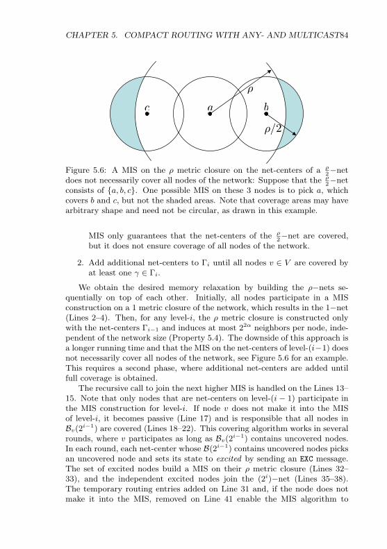
CHAPTER 5. COMPACT ROUTING WITH ANY- AND MULTICAST84
ρa bc
ρ/2
Figure 5.6: A MIS on the ρ metric closure on the net-centers of a ρ2−net
does not necessarily cover all nodes of the network: Suppose that the ρ2−net
consists of a, b, c. One possible MIS on these 3 nodes is to pick a, whichcovers b and c, but not the shaded areas. Note that coverage areas may havearbitrary shape and need not be circular, as drawn in this example.
MIS only guarantees that the net-centers of the ρ2−net are covered,
but it does not ensure coverage of all nodes of the network.
2. Add additional net-centers to Γi until all nodes v ∈ V are covered byat least one γ ∈ Γi.
We obtain the desired memory relaxation by building the ρ−nets se-quentially on top of each other. Initially, all nodes participate in a MISconstruction on a 1 metric closure of the network, which results in the 1−net(Lines 2–4). Then, for any level-i, the ρ metric closure is constructed onlywith the net-centers Γi−1 and induces at most 22α neighbors per node, inde-pendent of the network size (Property 5.4). The downside of this approach isa longer running time and that the MIS on the net-centers of level-(i−1) doesnot necessarily cover all nodes of the network, see Figure 5.6 for an example.This requires a second phase, where additional net-centers are added untilfull coverage is obtained.
The recursive call to join the next higher MIS is handled on the Lines 13–15. Note that only nodes that are net-centers on level-(i − 1) participate inthe MIS construction for level-i. If node v does not make it into the MISof level-i, it becomes passive (Line 17) and is responsible that all nodes inBv(2i−1) are covered (Lines 18–22). This covering algorithm works in severalrounds, where v participates as long as Bv(2i−1) contains uncovered nodes.In each round, each net-center whose B(2i−1) contains uncovered nodes picksan uncovered node and sets its state to excited by sending an EXC message.The set of excited nodes build a MIS on their ρ metric closure (Lines 32–33), and the independent excited nodes join the (2i)−net (Lines 35–38).The temporary routing entries added on Line 31 and, if the node does notmake it into the MIS, removed on Line 41 enable the MIS algorithm to

CHAPTER 5. COMPACT ROUTING WITH ANY- AND MULTICAST85
exchange messages on the optimal path between any two neighbors in thecorresponding metric closure.
For simplicity, we did not address the following issues in the pseudocodeof Algorithm 5.1.
• If a node v receives several EXC requests in the same round, it executesLines 30–42 only once, but finally acknowledges on Line 43 to all nodesthat sent the request.
• The net-centers need to obtain their enumeration values (see Chap-ter 5.3.2) in order to construct their labels. Because these labels areincomplete until all ρ−nets are constructed, the routing table entries(constructed on Lines 9, 25, 31, 37) are built using a partial labeling.
• The algorithm requires a rough synchronization between consecutiveMIS constructions, such that a MIS construction only starts when theprevious one finished. This can be obtained during the construction ofthe metric closure for the next MIS (Lines 14 and 32), where any nodecan ask the others to wait. To support this synchronization, each nodethat joined the ρ−net waits until all of its neighbors (in the metricclosure) have terminated the coverage procedure (Line 26).
• Whenever N = ∅ on Line 14, node v trivially joins the MIS and testswhether it covers all nodes of the network. If this is the case, v becomesthe root of the network and stops the recursive call to JoinMIS().
• Before the first MIS can be constructed, the nodes need to determinethe lowest cost associated with any edge of the network, as to determinethe scaling factor that scales this cost to 1.
Theorem 5.14. Algorithm 5.1 constructs a dominance net as described inChapter 5.3.1. Furthermore, the algorithm requires to build a total of at mostϑ(1 + 23α) = O(log Θ) MIS, which gives an upper bound on its running time.
Proof. We show the first property by induction on the levels: Initially, allnodes participate in a MIS election on the 1-metric-closure, which corre-sponds to building a MIS on the network where only the edges with cost 1are considered. By construction, the resulting MIS is a 1−net.
Given the points Γi−1 of a 2i−1−net, the algorithm first approximates Γiby a MIS on the 2i metric closure of Γi. By construction, a, b ∈ Γi =⇒dM(a, b) > 2i. Because only nodes that are not covered by Γi may becomeexcited (Line 19), the addition of any excited node to Γi does not breakthis property. Furthermore, the excited nodes added to Γi in one round areindependent with respect to the 2i metric closure on the set of excited nodes(Lines 32–34). Therefore, the minimum distance between net-centers of level-i is preserved. Because every γ ∈ Γi−1 repeats the completion process until

CHAPTER 5. COMPACT ROUTING WITH ANY- AND MULTICAST86
all nodes in Bγ(2i−1) are covered (Line 18), Γi finally covers all nodes and isa valid 2i−net.
As for the running time, we show that the algorithm may have to build atmost 1 + 23α MIS per level: The first MIS is built on Line 15, the remainingones on Line 33. Therefore, we need to show that a node v may executethe while-loop of Line 18 at most 23α times until all nodes in Bv(2i−1) arecovered. We first note that an excited node P (Line 19) may not join theMIS if another excited node Q with dM(P,Q) ≤ 2i joins. Therefore, anyexcited node Q that may interfere with P must lie in Bv(3 · 2i−1), and thenet-center that excited Q in Bv(2i+1). By Property 5.5, there are at most23α net-centers of level-i−1 in Bv(2i+1) and therefore at most 23α−1 excitednodes that may interfere with P . Just looking at P , we know that either Por one of its interfering nodes is selected in each round of the while loop.Thus, after at most 23α − 1 rounds, P can join the MIS, which shows thatat most 1 + 23α MIS are necessary per level. Because there are at most ϑlevels, the number of MIS to construct is bounded by ϑ(1 + 23α).

6Conclusion
In the preceding chapters we have described several routing protocols forwireless ad hoc networks. We started with a location service for mobilenetworks which is a prerequisite for any geographic routing approach whenthe nodes may change their position over time. The described protocol isnovel in the sense that we can show that messages are successfully deliveredeven if the destination node is constantly moving. The formalism introducedto prove this property, however, is based on rather strong model assumptionssuch as a dense node distribution, reliable communication, and the knowledgeof the position of lakes. In fact, by abstracting from the underlying routinglayer that forwards a message to a given position, we have hidden one of themost difficult tasks in dynamic networks. For example, consider Figure 6.1which depicts two networks A and B that are connected through two edgese1 and e2 and assume that a message needs to be routed from a node withinA to a node within B. In a worst case scenario, the two components arealways connected either by e1 or e2, but when the message is at a1, e1 is not
B
e1
a1
b1
A
e2 b
2a2
Figure 6.1: In a dynamic scenario, the two links e1 and e2 may come and goin a worst case fashion preventing communication between the two networkcomponents A and B.
CHAPTER 6. CONCLUSION 88
available. Similarly, if the message is at a2, the connection to b2 is broken.Thus, even though the two networks are constantly connected, it is hard toroute the message to its destination. Consequently, any protocol that wishesto provably ensure message delivery either needs to be able to detect andhandle such situations or it needs to be analyzed under a network modelthat prohibits such dynamic scenarios. But this raises the question on whatmodel should be chosen such that the model is simple enough to analyzethe protocols as well as realistic enough to represent the most importantproperties of wireless networks. Of course, the construction of simplifyingmodels is a tightrope walk and may not be possible at all without losing someimportant aspects. For instance, the UDG connectivity model abstracts fromtemporary link failures and the non-circular transmission range of physicalradios.
Despite of the theoretical nature of our results and their analysis undersomewhat strong models, we believe them to be a valuable starting point forfurther discussions and we hope that they may lay the basis for protocolstailored to more aspects of wireless networks, analyzed on more realisticmodels. For instance, many geometric routing algorithm for wireless ad hocnetworks were studied solely for 2-dimensional networks. In Chapter 3, wedescribed several randomized recovery techniques to escape local minimain 3-dimensional networks, which are by far more complex to handle thanin the 2-dimensional counterparts. Even though the fine grained analysisand the detection of the face was examined only under the simplified UBGconnectivity model, the results hold also for general graphs. Similarly, weshowed that any CUDG has a greedy embedding with constant stretch intoO`log2 n
´dimensions. Without the simplified network model, our approach
is still valid, but requires O`log3 n
´dimensions for the embedding and may
experience a stretch in O(logn). The compact routing result in Chapter 5was based on a networking model that seems to match the properties of awireless network better than the circular transmission radii of a UDG. Butthe construction of the labels and the routing tables suffers from the sameproblem as the construction of our greedy embedding: the labels cannot becomputed strictly locally and they hardly support network dynamics. Thus,there are still many open questions which we hope to see resolved in thecoming years.

Part IIApplication Design

7Simulation
The application development for distributed systems introduces new chal-lenges compared to the traditional application design. Most importantly,the actors of a distributed setup often need some means of coordination tocollaborate on a given task. Depending on the quality of the communicationmedium, a broad range of potential failures needs to be handled to guaran-tee a smooth operation, increasing the complexity of this coordination. Evenin the absence of such low-level failures, however, the design of distributedapplications remains challenging as it is often hard to foresee the interac-tion patterns between a (possibly large) set of concurrently executing actors.While hand-crafted toy examples give a basic insight into the applicationbehavior, they are limited to small systems and tend to be cumbersome.Computer aided simulations can help to quickly grasp the functioning ofa given protocol also in large settings, offering the possibility to verify thedesired behavior under a variety of operational conditions.
In this thesis, we consider wireless sensor networks which can be seen aslarge distributed systems: the sensor nodes collaborate to exchange messagesand perform the assigned surveillance tasks. For the design and validationof protocols for such sensor networks, we have developed sinalgo, a simula-tor for network algorithms that not only supports the development process,but is also suitable to run large scale simulations. We have used a prelim-inary version of sinalgo for the simulation of the MLS algorithm describedin Chapter 2.9. The simulations of the random walks on the dual graph inChapter 3.7 and the greedy embedding in Chapter 4.4 have been performedwith the final version available on sourceforge [39]. In all of our projects,the customizable visualization of sinalgo was helpful to understand and toperfect the algorithms before launching large scale batch simulations.

CHAPTER 7. SIMULATION 91
7.1 sinalgo
sinalgo offers a node-centric view of the network where each node may send amessage to a given neighbor or to all its neighbors, react to received messages,and set timers to schedule an action in the future. Similarly to real sensornodes, our software nodes are passive by default and act only upon receiving amessage or when one of their timers fires. Therefore, the core task of sinalgois to schedule message deliveries, fire timers, and advance the simulationtime. For more complex simulation scenarios, additional simulation modelscan be hooked up as needed. For instance, the simulation abstracts fromthe hardware layer and provides no real MAC layer. To simulate messageloss sinalgo provides several plug-ins to drop messages randomly or basedon a interference models such as the SINR model. The connectivity modelsdefine when two nodes are in communication range, UDG or QUDG arethe most prominent examples. Finally, mobility models describe how nodeschange their position over time, influencing indirectly the connectivity andinterferences models.
To allow for the greatest possible flexibility, each node holds its owninstance of a mobility, connectivity, and interference model. Thus, sinalgocan simulate networks consisting of nodes with heterogeneous properties.In addition to the described models, each node also implements a radioreliability model which may drop messages ad libitum. This model can beuseful to test an algorithm under the conditions of a lossy network withoutrequiring the computational overhead of a complete interference model.
The implementation of a given network protocol in sinalgo consists of thefollowing two steps: First, the properties of the network need to be definedby setting the appropriate models for the connectivity, mobility, and the in-terference. Furthermore, the desired amount of nodes must be deployed inthe simulation area according to a given placement model. As sinalgo alreadyships with an implementation of the most common models, this initial stepshould not require much work. In the second step, the behavior of the nodesmust be specified by implementing their reaction to received messages andfired timers. In addition, it must be defined how the progress of the algorithmis visualized and how the user can interact with an ongoing simulation. Asfor the visualization, nodes can be drawn with user defined shapes and colorsand may also display text. Figure 7.1 shows a screen shot of sinalgo whiledeveloping the routing algorithms on 3D networks of Chapter 3. This visual-ization tool not only enabled us to understand in more detail the constructionof the dual graph, but also facilitated the implementation and debugging ofthe simulation. To simplify user interaction at runtime, each node offers acontext sensitive pop-up menu through which arbitrary actions on the nodemay be initiated. Furthermore, the application code can be modified evenat run-time via hot-code replacement as sinalgo is written entirely in Java.

CHAPTER 7. SIMULATION 92
Figure 7.1: sinalgo in action showing the dual graph (light cubes) of a 3Dnetwork (bold lines). The customizable visualization can be used to displaycomplex constructs while the GUI’s rotation and zoom functions help tosee the third dimension. The right panel contains the simulation control,custom buttons for additional operations and logging output; it also showswhich part of the entire network is currently being displayed.

CHAPTER 7. SIMULATION 93
Algorithm 7.1: Synchronous simulation round
Increment Time The time advances by 1 unit1
PreRound Simulation specific initializations for this round2
Mobility Move each node according to its mobility model3
Connectivity Recompute the connections4
Interference Drop messages that experience too much interference5
On each node:6
Receive messages7
Handle fired timers8
PostRound Simulation specific cleanup code for this round9
These two tools turned out to be convenient for testing special cases anddifferent versions of an algorithm.
7.2 Simulation modes
The sinalgo simulator offers two simulation modes: a synchronous roundbased simulation and an asynchronous event driven simulation. In the lat-ter, each event (a message reception or the firing of a timer) executes at a welldefined time. sinalgo only needs to temporally order these events and executethem sequentially. Whereas an asynchronous simulation mode reflects wellthe asynchronous nature of wireless networks, it also breaks up the algorithmin its atomic pieces, making it harder to grasp the overall picture. For thisreason, algorithms are often designed and analyzed in a round based model,where the algorithm advances in rounds. In this model, the time advancesin discrete steps from round to round and the nodes perform their actionssynchronously during these rounds. I.e. a message sent in round i arrives atthe earliest in round i+ 1. Algorithm 7.1 shows the actions sinalgo performsin each round: After initializing the round in Line 2, the mobility and con-nectivity models move and reconnect the nodes and the interference modeldrops messages if necessary (Lines 3–5). After this step, sinalgo iterates overall nodes to signal message receptions and the firing of timers (Lines 7,8).Please note that the order in which the nodes are processed is not importantas messages sent within this round will arrive at the earliest in the followinground. Finally, the round is concluded on Line 9 to perform cleanup andlogging operations specific to the simulation.
7.3 Mobility
The simulation of mobile nodes is quite involved if continuous paths shouldbe analyzed, especially in combination with interference and connectivity
CHAPTER 7. SIMULATION 94
models which are based on the geometry of the network. Therefore, sinalgooffers only a simplified node mobility where the nodes move in discrete steps.In the synchronous simulation mode, the nodes are moved according to theirmobility model at the beginning of each round (Line 3 of Algorithm 7.1)such that the following connectivity check can reestablish connections. Ifnecessary, a finer resolution of the moved paths can be obtained by advancingthe time in each round by a smaller amount (Line 1). Consequently, messagesneed more rounds until they are delivered and are therefore tested severaltimes for interference and dropped connections. For most simulations ofmobile networks, however, the default resolution is enough, as messages mayalso be dropped through the reliability model, simulating message loss dueto arbitrary effects. In contrast to the synchronous mode, sinalgo does notsupport mobility in the asynchronous simulation mode. A discrete mobilitycould be implemented, but we did not want to break the purely event drivenscheme.
The simulation of mobile networks is computationally involved as eachnode constantly needs to validate its connections and establish links to nodesthat have moved into its communication range (Line 4). For general connec-tivity models, all node pairs need to be compared, costing O
`n2´
operations,where n is the number of nodes. But as we mostly consider geometric net-works where the connectivity depends on the distance between nodes, wecan bring down this overhead to O(n · d), where d is the expected node de-gree. To achieve this performance gain, sinalgo stores the nodes accordingto their position such that range queries can be answered efficiently. For 2Dnetworks, the deployment area is subdivided into a quadratic grid with a cellside length of rmax, the maximum transmission range of the nodes. For eachof these grid cells, sinalgo remembers which nodes are located within the cell.Therefore, all neighbors of a node located in a cell c are either in c or one ofthe 8 cells adjacent to c. Similarly, 3D networks are subdivided into cubicgrids of side length rmax such that a set of potential neighbors can be foundefficiently.
7.4 Discussion
sinalgo is a simulation tool for testing and validating wireless network pro-tocols. It is written in Java and ships with a set of common operationalmodes such that the initial overhead to prototype a protocol is low. For abasic simulation, it is sufficient to implement only the behavior of the nodesbefore gradually fine tuning the simulation by customizing the simulationmodels, the run-time environment, or the visualization. To obtain an effi-cient framework, sinalgo operates on a message passing model that abstractsfrom the physical properties of hardware devices. As a result, sinalgo onlyprovides limited support for the simulation of MAC layers. For simulations

CHAPTER 7. SIMULATION 95
that should consider the entire networking stack, the ns-2 simulator for wire-less networks [74] is a widely used option. In contrast to sinalgo, however,ns-2 focuses on the simulation and provides less support for the developmentprocess, e.g. there is only a trace-based visualization that displays the in-teractions after the simulation finished. The simulation tool most similar tosinalgo is Shawn [55] which also abstracts from the networking layer to focuson the protocol implementation. Shawn is written in C++ and outclassessinalgo in terms of performance when simulating huge networks. On thecontrary, sinalgo offers more visualization options and interaction with anongoing simulation.
Independent of the simulation tool in use, we need to keep in mind that nosimulation replaces a real experiment, especially in wireless networks wherethe operational conditions often change over time. In addition, it is oftenhard to predict how good simulation results match reality, especially if thesimulation was based on simplistic models. For instance, sinalgo offers theconvenient round based simulation mode where nodes advance synchronouslyto perform their actions in parallel. This viewpoint helps to describe the al-gorithms in a simpler form hiding the asynchronous nature of distributedhardware. However, it raises the question on how such a synchronous proto-col can be implemented on hardware after a successful simulation. In fact,the transition from a simulation prototype to the hardware implementationis challenging as any adaptation of the code must be verified to not breakthe overall behavior. The TOSSIM emulator [62] for TinyOS applicationsavoids this problem by using the same code base for the simulation as wellas for the device. To generate the simulation, TOSSIM requires a specialcompilation procedure which redirects hardware calls to the simulation coreof TOSSIM which then simulates the corresponding interrupts to keep thesystem running. Whereas this tool is great to emulate code prior to deploy-ment, it requires the protocols to be written in nesC and the applicationmust already be tailored to a specific hardware platform. But both, the Clanguage and the platform dependence are highly undesirable for prototyp-ing and testing new protocols, rendering high level simulation tools such assinalgo attractive.
To facilitate the transition between a simulation and the implementa-tion for the hardware, we have studied how to port synchronous protocols toasynchronous hardware such as our sensor nodes. In fact, the synchronousapproach not only facilitates simulations, but would also be handy for thedevice software as the different steps of the protocols are automatically sep-arated and synchronized, giving the execution an implicit structure. Wepresent first steps towards this goal in the remaining chapters of this thesis.In particular, we propose a novel programming paradigm that challenges thetraditional asynchronous applications with a synchronized execution envi-ronment where the nodes perform their operations in a series of synchronous

CHAPTER 7. SIMULATION 96
time slots. Even though our system does not work exactly as the synchronoussimulation mode described in Algorithm 7.1, we believe it to be powerfulenough to ease the implementation of protocols that were initially designedin a synchronous context.

8Slotted Programming
After the design and simulation of novel protocols for wireless networks,they need to be implemented on the hardware devices. This final step oftenrequires a major redesign of the program code used for the simulation, ashardware specific constraints need to be taken into account. In this chapter,we focus on the software development for wireless sensor networks and presenta novel programming style to facilitate this rather involved task.
In general, software for distributed systems tends to be “heavy”, con-sisting of several components and layers that interact with each other in anon-trivial way to cope with various transient or permanent failures and mostlikely also some kind of dynamics. The icing on the cake is the whole pro-cess of software development, e.g. issues such as debugging between remotenodes. But programming embedded systems is no picnic either. Embeddedsystems ask for “light” software that does not waste resources such as mem-ory, processing power, or energy. In addition, the systems often need to meettight run-time requirements and guarantee a predictable execution. Againthe software development cycle is tedious, as the programmer does not havedirect access to the hardware, but must go through cross-compilation andcross-debugging.
Wireless sensor networks clearly inherit all the problems from networkeddistributed systems as well as embedded systems. To make matters worse,running “heavy” distributed systems software on “light” embedded systemshardware sounds like an insurmountable contradiction at first. However,sensor networks can be done. While early deployments have suffered in termsof bad reliability, high energy consumption, or bad scalability, more recentdevelopments overcome these issues with novel algorithms such as energy-efficient MAC protocols [51, 90, 100] which can be tuned to suit a givenapplication best.
The work to build such energy efficient protocols and applications shallnot be underestimated. Current energy efficient implementations need to be

CHAPTER 8. SLOTTED PROGRAMMING 98
optimized across the entire application. This comes at the price of a non-modular design. Adding further functionality may require drastic changes incode, and even small adaptations to parameters or changes of the environ-ment may trigger a serious investment in re-testing.
Not surprisingly, there is a trend towards simplifying and standardiz-ing the programming environment. Some proposals abandon the idea ofenergy efficient hardware altogether, and instead advocate a Linux or JavaVM framework [15, 49, 85]. Some other proposals [51] envision an IP layerhiding a general purpose low-power networking stack. Clearly, all these ef-forts are fine for rapid prototyping. However, as we will argue later in thischapter, these abstractions are not suitable for real-world implementations.For instance, the energy efficiency of many applications could be improvedby an order of magnitude when writing special purpose communication pro-tocols. In addition, the abstractions hide the complexity of the underlyingimplementation. This is dangerous especially for time sensitive tasks, wherehardware devices such as the CPU or the radio must be available exactly ata given time.
In this chapter we outline the slotted programming paradigm which sup-ports both modularity and energy-efficiency. This programming approach isnot orthogonal to the current trend of providing high level abstractions. Itrather extends the abstractions with a predictable execution scheme, givingback full control to the application developer. Our concept is simple: Weconsider the different tasks of a sensor node such as clock synchronization,routing, topology control, sensing, or code updates. Each of these tasks isgiven time slots during which it performs its operations in parallel on allnodes. The time slots need to be assigned in a non-overlapping way suchthat at any time, at most one task executes its code. If a job has not ter-minated at the end of its assigned time slot, it must be suspended and mayonly continue its execution during its next time slot. Thus, tasks do notinterfere with each other, and they do not interrupt each other. Therefore,each task can be implemented as an independent module which can be ex-changed easily. Indeed, alternative modules for the same task can be testedand compared within the same application. Moreover, different modules cancommunicate with incompatible packet formats, e.g. IPv6 packets vs. AM-packets, as they will not disturb each other. In fact, we will demonstratein Chapter 10 that it is even possible to use the radio in radically differ-ent ways, e.g. packets vs “waves”. All in all, we believe that our approachfosters modular programming where modules can be exchanged easily. Inaddition, we show that also modular applications allow for highly optimizedand energy efficient code. For instance, our clock synchronization describedin Chapter 9 turns on the radio only for 0.06% of the time even though itreceives and sends one message every 32 seconds.

CHAPTER 8. SLOTTED PROGRAMMING 99
8.1 Related Work
The application development for sensor networks combines techniques fromembedded systems, networking, and also real time systems. To support thisdelicate task, dedicated operating systems were built already in the earlydays. The most prominent OS is TinyOS [92], which was a purely eventdriven framework supporting many hardware platforms. Over time, TinyOSwas extended with new features to ease application development and reduceprogramming errors. Most recently, a safe type-system [23] and support formulti-threaded programming [71] were added.
However, the quest for an optimal programming environment was notonly led by TinyOS. For instance, the MANTIS OS [1] supported preemp-tive multi-threading well before TinyOS did, and Contiki [28] is based onlightweight protothreads [29]. The notion of virtual memory was introducedin the t-kernel [46] to protect the operating system from being corrupted bythe user application, and SOS [48] supports the dynamic loading of modules,avoiding the static linking at compile time. All operating systems above arebased on the low level C programming language or a dialect thereof, butthere have been efforts to support Java [15, 49, 85], requiring the nodes torun a virtual machine to execute the byte-code.
Besides these low-level OS developments, explicit support for energyaware programming was proposed. Whereas Nano-RK [35] is a real-timeoperating system with static resource allocation, the pixie OS [67] allowsfor a dynamic resource allocation at runtime, predicting the energy draw ofthe operations in an online fashion. As the radio is among the primary en-ergy consumers, much work has also been put into building energy efficientcommunication protocols. In asynchronous low power listening schemes suchas WiseMAC [32] or B-MAC [79], each node periodically samples the radiofor packet announcements. Whenever a node wishes to send a message, itfirst sends a rather long preamble to announce the forthcoming packet. X-MAC [17], SCP-MAC [100], RI-MAC [90] and [51] outline several approachesto reduce this overhead. TP-MAC [44] is probably the most related work toour signaling described in Chapter 10. The authors of [44] propose a pipelinedwake-up schedule but do not consider interference. We extend this idea andprovide an interference resilient signaling which we also tested on real hard-ware. To the best of our knowledge, this work is the first to describe andimplement a fully functional wake-up signaling that is resilient to interfer-ence.
To reduce the learning curve and simplify the development of sensornetwork applications, TinyOS and other operating systems support multi-threaded programs. Furthermore, low power listening protocols can be usedto provide a basic MAC layer to the application developer. In fact, Hui andCuller [51] envision a IPv6 stack on top of such a MAC layer to hide theunderlying networking to the application developer. We embrace this trend

CHAPTER 8. SLOTTED PROGRAMMING 100
towards a standardized communication framework and believe it to be per-fect for prototyping sensor network applications. However, when it comesto the development of real-world applications, we would like to express ourreservation to this approach for several reasons. Firstly, the execution ofa multi-threaded application is hard to predict. As a result, the develop-ment and also debugging is much more involved as some errors may occuronly sporadically under a specific preemption. Similarly, the introduction ofa networking abstraction such as a low power listening MAC introduces arather unpredictable use of the CPU and the radio device, possibly delay-ing other tasks. Thus, the developer does not have complete control overthe application, which makes it hard to ensure a bug-free program. Lastbut not least, the resulting applications are by far not as energy efficientas they could be. For instance, the task of collecting a message from ev-ery node once a minute causes a duty-cycle of 0.65% with the IPv6 networkstack of [51]. In Dozer [18], a data gathering protocol with a dedicated MAClayer, a message was collected every 30 seconds. The duty-cycle for thistask was reported to be only 0.167%, reducing the overhead by a factor of8. However, this improvement comes at the price of a higher latency anda completely asynchronous application that is hard to maintain. For com-parison, our clock synchronization algorithm described in Chapter 9 receivesand sends one message every 32 seconds and requires an average duty-cycleof only 0.06%. Of course, these numbers cannot be compared directly, butthey indicate that there is still a lot of potential for saving energy. With theslotted programming paradigm, we demonstrate that it is indeed possible towrite modular applications that are also energy efficient.
8.2 Background
Access to the different hardware components such as the radio module,timers, flash chip, or the sensors is often done through software arbitrationor the explicit knowledge that no other code fragment is using the desiredcomponent. Clearly, the latter approach is not only prone to undetected con-flicts, but also renders code reuse a nightmare. But software arbitration aloneis not enough to write modular applications as we outline in the followingpoints.
Real time applications The load of the CPU is hard to predict, as otherpieces of the application may require computational complex tasks at anytime. As a result, tasks and synchronous events may execute with a non-negligible delay, which poses problems to the implementation of time criticalapplications where some actions should happen exactly at the prescribedtime. This is in sharp contrast to classic real time systems, where the tasksshould execute within a larger time window before a given deadline. For
CHAPTER 8. SLOTTED PROGRAMMING 101
instance, even the simple task of enabling the radio on two neighboring nodesat exactly the same time is hard to achieve, as any of the nodes may beoccupied with other tasks and therefore delay the power-on command.
A common approach to suppress this problem is to introduce a guard-time, which specifies how much before the arranged time the radio should beturned on. Apart from the fact that it is hard to predict good guard-times,applications use more energy than necessary and also gain in complexity.
Alternatively, the radios could be powered on in an asynchronous codeblock, ensuring instantaneous execution if no other asynchronous event in-terferes. However, implementations which rely on preemptive code execution(e.g.[18]) are quite hard to maintain, as any modification or extension mayaffect any other part of the system. As such asynchronous systems are oftenvery complex and even the slightest anomaly in the code can lead to misbe-havior such as memory corruption or even a deadlock, we believe that thisapproach should be avoided whenever possible.
Multi-threaded operating systems are not improving the situation, as theyeven explicitly permit preemption of tasks, delaying operations even further.Prioritization of the threads does not resolve the problem, as the thread withthe lower priority still experiences a delay.
Modularity In most sensor network scenarios, each network node needsto fulfill several tasks, e.g. clock synchronization, sense the environment,process the measurements, and disseminate the sensed data. To obtain ahighly optimized application that uses as little energy as possible, the usualapproach is to combine the required tasks as well as possible. In our example,this could mean that the messages required for the clock synchronization arepiggybacked onto the data gathering messages or vice versa. Whereas suchan implementation can be very energy efficient, it is also highly specific to thegiven problem instance. Therefore, any modification or extension needs totake into account the entire application, and partial code reuse in a differentapplication is cumbersome.
Incomplete algorithm design We have already argued that any twotasks running in parallel may interfere by reducing the responsiveness of thenode. Similarly, the software arbitration may temporarily block the accessto a hardware resource such as the radio module while another task is usingit. Also, if two hardware components happen to be connected to the CPUthrough a shared bus, at most one of them may be accessed at any time. Thisis the desired behavior, but it is often difficult or even impossible to predictsuch conflict patterns. Therefore, algorithms for sensor nodes are normallydesigned under the simplifying assumption of immediate access to the hard-ware, ignoring the fact that another task may run in parallel competing forthe same resources. Adapting these algorithms to the existing hardware con-
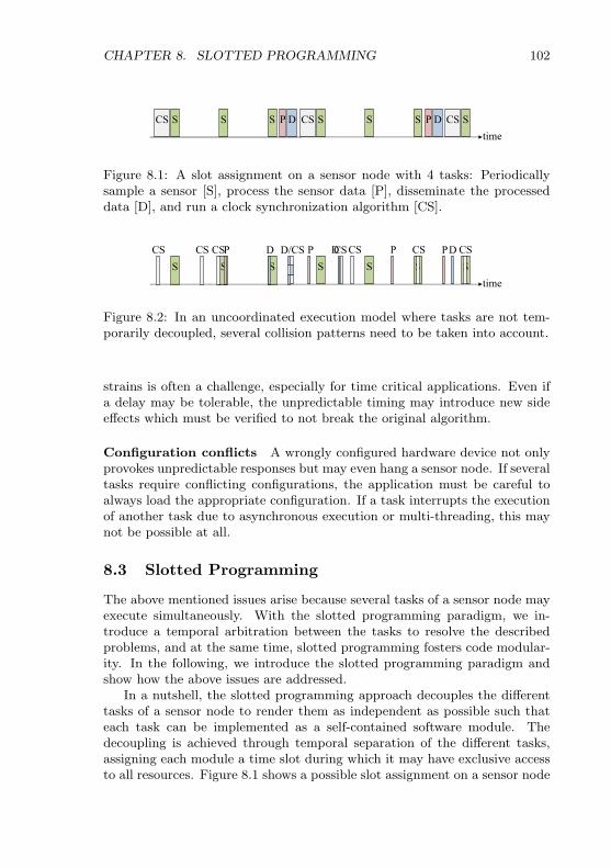
CHAPTER 8. SLOTTED PROGRAMMING 102
time
S CS S S S S S CSP D CSP D S
Figure 8.1: A slot assignment on a sensor node with 4 tasks: Periodicallysample a sensor [S], process the sensor data [P], disseminate the processeddata [D], and run a clock synchronization algorithm [CS].
time
S S S S S S S
P DCS
D/CS
P P P
D D
CS
CS CS
CS CS
CS
Figure 8.2: In an uncoordinated execution model where tasks are not tem-porarily decoupled, several collision patterns need to be taken into account.
strains is often a challenge, especially for time critical applications. Even ifa delay may be tolerable, the unpredictable timing may introduce new sideeffects which must be verified to not break the original algorithm.
Configuration conflicts A wrongly configured hardware device not onlyprovokes unpredictable responses but may even hang a sensor node. If severaltasks require conflicting configurations, the application must be careful toalways load the appropriate configuration. If a task interrupts the executionof another task due to asynchronous execution or multi-threading, this maynot be possible at all.
8.3 Slotted Programming
The above mentioned issues arise because several tasks of a sensor node mayexecute simultaneously. With the slotted programming paradigm, we in-troduce a temporal arbitration between the tasks to resolve the describedproblems, and at the same time, slotted programming fosters code modular-ity. In the following, we introduce the slotted programming paradigm andshow how the above issues are addressed.
In a nutshell, the slotted programming approach decouples the differenttasks of a sensor node to render them as independent as possible such thateach task can be implemented as a self-contained software module. Thedecoupling is achieved through temporal separation of the different tasks,assigning each module a time slot during which it may have exclusive accessto all resources. Figure 8.1 shows a possible slot assignment on a sensor node

CHAPTER 8. SLOTTED PROGRAMMING 103
Slot Scheduler
Clock
Sync
Module
M1 M2 Mi M3 . . .
Figure 8.3: Schematic view of a slotted system: The slot scheduler starts andstops the software modules, the clock synchronization module is responsiblefor obtaining the network time.
with 4 distinct tasks. This is in sharp contrast to an uncoordinated executionmodel, where tasks my collide and experience unpredictable side effects asillustrated in Figure 8.2.
8.3.1 The Basics
The slotted programming paradigm builds on a synchronous execution model.It requires that all nodes have a global notion of time, i.e. they need to runsome kind of clock synchronization algorithm. This network time is used toschedule the execution of the software modules, such that the same softwaremodule executes simultaneously on all nodes.
Each task of a sensor node is implemented as an independent softwaremodule providing the desired functionality. E.g. there may be a clock syn-chronization module, a data gathering module, a sampling module, and adata processing module. To obtain the temporal decoupling with other soft-ware modules, each software module must ensure that its code executes onlywithin an assigned time slot and that it causes no side effects outside thisslot.
The software modules are then integrated into the slotted system by allo-cating time slots for each of them. Whereas arbitrary complex schedules canbe built, simple periodic schedules similar to the one shown in Figure 8.1 arealready sufficient for most applications. The only restriction for the overallschedule is that there may be no region where slots overlap, otherwise thetemporal decoupling would be broken. Depending on the scheduling com-plexity, this property can already be tested at compile time. Alternatively, arun-time check may be applied.
The basic support for slotted programs is provided by two components:A clock synchronization module and a scheduler module. The latter executesthe desired schedule by signaling each module the start and end of its timeslots. Figure 8.3 illustrates a schematic view of a slotted system. Interesting

CHAPTER 8. SLOTTED PROGRAMMING 104
to note is the tight coupling of the clock synchronization module and theslot scheduler: Whereas the slot scheduler depends on the network time toschedule the modules, the clock synchronization module itself is scheduledby the slot scheduler. This circular dependency is no problem as soon as thenode is roughly synchronized, but special care needs to be taken while a nodeis not synchronized. See Chapter 8.4.2 for more details on this topic.
8.3.2 Guidelines for Slotted Programming
Given an operating system that provides the basic functionality for slottedprogramming (clock synchronization and a slot scheduler), the developmentof a sensor node application boils down to the following three steps:
(A) Modularization of the application. In this preliminary software designstep, we identify the tasks which can be implemented as self-containedsoftware modules. This first step intentionally leaves open a broadrange of design decisions such as to not restrict the programmingparadigm to a narrow field of applications. The focus of this step,however, should be on the reusability of the individual modules andon the temporal decoupling of the implemented tasks.
(B) Implementation of each individual module. First, define the time slotsduring which the given module is allowed to operate. Whenever pos-sible, this choice should be parametrized such that an overall schedulecan be obtained easily when assembling several modules (see below).The implementation of the module must ensure that its code onlyruns between the startSlot() and stopSlot() events generated by theslot scheduler.
(C) Determine an overall schedule. The integration of the desired modulesrequires a non-overlapping scheduling of all time slots. Ideally, eachmodule parametrizes the execution time of its time slots, such that theglobal schedule can be obtained by tuning these parameters. When themodules adapt their schedule dynamically at runtime, this task mayquickly become quite complex. But as periodic schedules are sufficientfor most applications, a valid schedule can often be found quickly.
8.3.3 Discussion
With the slotted programming paradigm, we foster modular programs forsensor nodes. The key component is the temporal decoupling of moduleswhich guarantees that at any time, at most one module is running its codewithout being preempted. This decoupling lays the basis for the followingproperties of slotted programming:
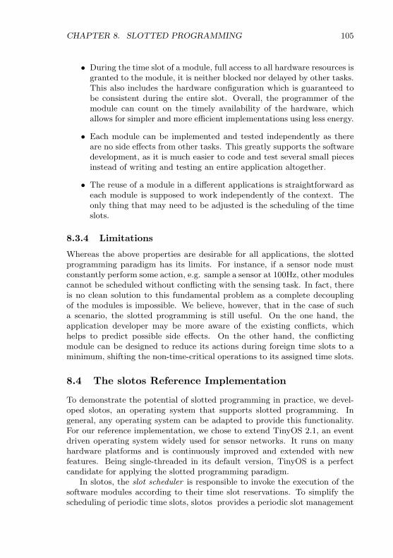
CHAPTER 8. SLOTTED PROGRAMMING 105
• During the time slot of a module, full access to all hardware resources isgranted to the module, it is neither blocked nor delayed by other tasks.This also includes the hardware configuration which is guaranteed tobe consistent during the entire slot. Overall, the programmer of themodule can count on the timely availability of the hardware, whichallows for simpler and more efficient implementations using less energy.
• Each module can be implemented and tested independently as thereare no side effects from other tasks. This greatly supports the softwaredevelopment, as it is much easier to code and test several small piecesinstead of writing and testing an entire application altogether.
• The reuse of a module in a different applications is straightforward aseach module is supposed to work independently of the context. Theonly thing that may need to be adjusted is the scheduling of the timeslots.
8.3.4 Limitations
Whereas the above properties are desirable for all applications, the slottedprogramming paradigm has its limits. For instance, if a sensor node mustconstantly perform some action, e.g. sample a sensor at 100Hz, other modulescannot be scheduled without conflicting with the sensing task. In fact, thereis no clean solution to this fundamental problem as a complete decouplingof the modules is impossible. We believe, however, that in the case of sucha scenario, the slotted programming is still useful. On the one hand, theapplication developer may be more aware of the existing conflicts, whichhelps to predict possible side effects. On the other hand, the conflictingmodule can be designed to reduce its actions during foreign time slots to aminimum, shifting the non-time-critical operations to its assigned time slots.
8.4 The slotos Reference Implementation
To demonstrate the potential of slotted programming in practice, we devel-oped slotos, an operating system that supports slotted programming. Ingeneral, any operating system can be adapted to provide this functionality.For our reference implementation, we chose to extend TinyOS 2.1, an eventdriven operating system widely used for sensor networks. It runs on manyhardware platforms and is continuously improved and extended with newfeatures. Being single-threaded in its default version, TinyOS is a perfectcandidate for applying the slotted programming paradigm.
In slotos, the slot scheduler is responsible to invoke the execution of thesoftware modules according to their time slot reservations. To simplify thescheduling of periodic time slots, slotos provides a periodic slot management

CHAPTER 8. SLOTTED PROGRAMMING 106
Time
0
128 [s]
256
348 512
Figure 8.4: The slot scheduler repeats a partial schedule generating a periodicexecution of the allocated time slots.
Interface 8.1: Slot scheduler interfaceevents
void init()void startSlot(slotID, slotCmd, syncQuality, syncStatus)void stopSlot(slotID)
commandsslotID addTimeSlot(startTime, length, slotCmd)void modifyTimeSlot(slotID, startTime, length, slotCmd)bool testSchedule()
void stopScheduling()void continueScheduling()...
with an allocation window of 128 seconds. Each module allocates its timeslots within this allocation window which is repeated periodically by the slotscheduler to obtain the overall schedule, see Figure 8.4 for an example. Withthis scheduling approach, slotos facilitates the allocation of periodic timeslots which we believe to be sufficient for most applications. The size ofthe allocation window is currently set to 128 seconds, but it may be set towhatever fits best the application needs. For more sophisticated schedules,the dynamic time slot reservation of slotos may be used to reorganize theschedule at run-time.
Interface 8.1 sketches the interface of the slot scheduler. During theinit() event, which is called upon booting the node, each module allocatesits time slots. addTimeSlot() is used to reserve an additional time slot, andmodifyTimeSlot() reschedules an existing time slot. Whenever a time slotstarts, the startSlot() event is signaled on the corresponding module indi-cating an estimate of the current synchronization quality. Finally, the end ofthe slot is signaled by the stopSlot() event.
CHAPTER 8. SLOTTED PROGRAMMING 107
8.4.1 Policy Enforcement
The temporal decoupling of the modules is the key of slotted programming.Whereas a static schedule can be checked at compile-time to have no over-lapping regions, dynamically generated schedules can only be verified atrun-time. slotos implicitly detects overlapping time slots and refrains fromscheduling them simultaneously. Instead, it provides a best-effort service de-laying the start of the later time slot until the end of the active time slot. It isimportant to note that this error handling approach should not be exploitedas a feature of the slot scheduler. It is rather a last resort to guarantee acontinuous execution of all reserved time slots, based on the assumption thatthe broken schedule is only of temporal nature.
In addition to a non-overlapping schedule, the temporal decoupling alsorequires that the software modules operate only during their assigned timeslots. This property, however, is much harder to verify or even enforce, asthe modules should be allowed to execute arbitrary actions within their timeslots. For instance, a module may set a timer to fire outside its time slot orinitiate a split phase command whose callback returns only after the time slotterminates. Whereas the timer issue can be addressed by cancelling timersthat are set outside the current time slot, callbacks from the hardware aredevice specific and often hard to predict. The current implementation ofslotos does not try to detect or avoid activity outside the assigned time slotsand requires the module developer to adhere strictly to the time constraints.Thus, slotos does not enforce slotted programming but only provides a suit-able execution environment.
8.4.2 Clock Synchronization
Clock synchronization is an integral part of slotos; it ensures that the softwaremodules are scheduled simultaneously on all nodes. Its task is to maintain theclocks synchronized with neighboring nodes and react to topology changeswhich may leave the node unsynchronized for an arbitrary amount of time.
As clock synchronization is implemented as a self-contained module, itneeds to be scheduled by the slot scheduler, but the slot scheduler itselfrelies on the synchronization. slotos supports two approaches to break thiscircular dependency.
(A) The clock synchronization module may temporarily turn off the slotscheduler. During this time, no other module is scheduled to executeand the synchronization module is free to access the radio for an ex-tended time to receive synchronization messages. Once an approximatesynchronization is available, the slot scheduler can be turned on again.
(B) It is often undesirable to completely shut down the slot scheduler asthis also stops any other activity on the sensor node, including the
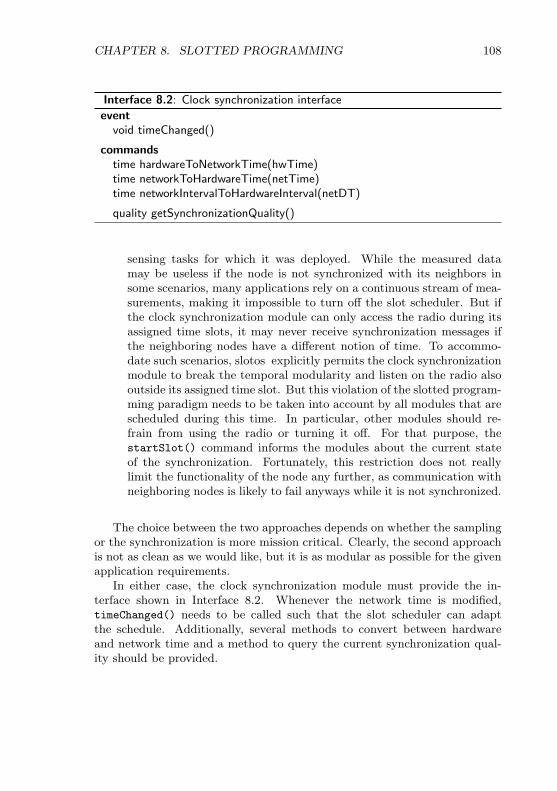
CHAPTER 8. SLOTTED PROGRAMMING 108
Interface 8.2: Clock synchronization interface
eventvoid timeChanged()
commandstime hardwareToNetworkTime(hwTime)time networkToHardwareTime(netTime)time networkIntervalToHardwareInterval(netDT)
quality getSynchronizationQuality()
sensing tasks for which it was deployed. While the measured datamay be useless if the node is not synchronized with its neighbors insome scenarios, many applications rely on a continuous stream of mea-surements, making it impossible to turn off the slot scheduler. But ifthe clock synchronization module can only access the radio during itsassigned time slots, it may never receive synchronization messages ifthe neighboring nodes have a different notion of time. To accommo-date such scenarios, slotos explicitly permits the clock synchronizationmodule to break the temporal modularity and listen on the radio alsooutside its assigned time slot. But this violation of the slotted program-ming paradigm needs to be taken into account by all modules that arescheduled during this time. In particular, other modules should re-frain from using the radio or turning it off. For that purpose, thestartSlot() command informs the modules about the current stateof the synchronization. Fortunately, this restriction does not reallylimit the functionality of the node any further, as communication withneighboring nodes is likely to fail anyways while it is not synchronized.
The choice between the two approaches depends on whether the samplingor the synchronization is more mission critical. Clearly, the second approachis not as clean as we would like, but it is as modular as possible for the givenapplication requirements.
In either case, the clock synchronization module must provide the in-terface shown in Interface 8.2. Whenever the network time is modified,timeChanged() needs to be called such that the slot scheduler can adaptthe schedule. Additionally, several methods to convert between hardwareand network time and a method to query the current synchronization qual-ity should be provided.

CHAPTER 8. SLOTTED PROGRAMMING 109
8.4.3 Timers
It is often the case that two neighboring nodes wish to wake up simultaneouslyto exchange messages or perform other operations. Slotted programs supportsuch interactions as the software modules are scheduled simultaneously onall nodes. Thus, it is sufficient for a module to set a timer to be waken up atthe arranged time. To obtain a truly decoupled system, the modules shouldrespect the following guidelines when setting timers:
• Most importantly, timers may only be set to fire within the currenttime slot. If a timer should fire during a later time slot, the moduleshould remember this and start the timer only at the beginning of thedesired time slot. Thanks to this restriction, timers never need to beupdated to reflect a modified network time because no timer is activewhen the clock synchronization module resets the network time.
• Whenever possible, timers should be started relative to the start timeof the current time slot. This results in a more precise timing thanwhen using offset timers, as their fire time depends on the time whenthey are set. In TinyOS, this can be done using the startOneShotAt()
method of the Timer interface.
• Interactions with other nodes should be arranged based on the commonnetwork time. The timers in slotos, however, operate on the localtime of the node, requiring a conversion from the network time to thecorresponding local time. The methods offered by the synchronizationmodule can be used for this conversion, see Interface 8.2.
• To account for fluctuations of the clock synchronization, a module mayapply guard times to ensure that it does not miss an arranged meeting.In the case of a scheduled message transmission, the receiver wakes upa bit earlier and the sender sends the message a bit later to ensurethat the two meet. The estimation of the clock synchronization passedon in the startSlot() event may be used to adaptively set the guardtimes.
In the following we demonstrate the advantages of the slotted program-ming approach at two applications. We start by describing the design andimplementation of a slotted time synchronization module in Chapter 9. InChapter 10, we describe a novel signaling technique which can be used topropagate alarms efficiently and reliably through a network. While the sig-naling technique itself is of interest, the simplicity of its integration into ourtest application demonstrates the power of slotos.

9Slotted Clock Synchronization
As clock synchronization is a central part of slotos and slotted programmingin general, we now describe in more detail the clock synchronization modulethat comes with slotos. Being implemented itself as a software module, weuse this synchronization module to demonstrate the advantages of the slottedprogramming paradigm.
Due to its simplicity, we provide a variant of the FTSP algorithm [70]where an elected root node dictates its time to the remaining nodes. Incontrast to the original FTSP algorithm, we apply a simplified version thereofwhere a dedicated root node dictates its time to the remaining nodes. Nodesin the immediate neighborhood of the root node learn the network timedirectly from the root node. Once a node is synchronized, it disseminatessynchronization messages itself such that nodes not directly connected to theroot synchronize indirectly. Each node selects a single parent node to which itsynchronizes, resulting in a tree algorithm. Furthermore, our synchronizationalgorithm relies on a static root node. Whereas our implementation is notreally fine-tuned and experiences an average synchronization error of 44µs perhop, this is already sufficient for many applications. In fact, as our hardwaretimers are based on a rather slow 32.768 kHz oscillator, it is hard to obtaina synchronization error below one time unit (30µs). Overall, we focused onobtaining an energy efficient solution rather than a perfectly synchronizedsystem.
slotos offers a time window of 128 seconds to schedule the execution ofthe software modules. Our clock synchronization module reserves 4 time slotsof 1 second in regular intervals such that the module is launched every 32seconds, see Figure 9.1. Within these assigned time slots, the module mayperform any actions as the slotted programming guarantees that no othertask interferes. In our case, the module only needs to receive a sync messagefrom its parent and to broadcast a sync message for its children.

CHAPTER 9. SLOTTED CLOCK SYNCHRONIZATION 111
t
0 12832 64 96
Clock Sync
38 37 39 40 41
Figure 9.1: The default clock synchronization module of slotos allocates 4time slots of 1 second. The time slots are spread over the allocation windowof the slot scheduler such that the module is invoked every 32 seconds. Theremaining time slots can be used arbitrarily by other software modules.
9.1 Synchronized Transmission
In order to avoid collisions, each node chooses its transmission time of thesync message randomly within the assigned time slot. In each transmittedmessage, the sender includes the seed value of the random number generatorthat will be used to send forthcoming sync messages. From this information,the receiving child can predict when its parent sends the next sync messageand enable its radio just for the required time period. The child can evenpredict the arrival of a sync message when it has missed several messagesin between. This is possible as we use a circular random number generatorwhere the generated number is used as the seed for the following draw.
Synchronization fluctuations render it impossible for the receiver to wakeup just in time to receive the message. We apply an adaptive guard timewhich is decreased for each successful reception and increased otherwise. Thisleads to a close to optimal message reception overhead, ensuring low energyconsumption.
9.2 Pipelined Synchronization
When sending the sync message at a random time within the assigned slot,a child may forward its sync message before receiving the sync message fromits parent. As a result, the sync message sent by the child may be inaccurateas it is based on a synchronization which is at least 32 seconds old. Toovercome this issue, our implementation pipelines the transmission along thesynchronization tree. The synchronization module achieves this by dividingits time slot into k cells of equal length (see Figure 9.2) and restricting thetransmission of the sync message to one specific cell. This cell assignmentis based on the number of hops the node is away from the root node (onthe synchronization tree). A node which is h hops away from the root node

CHAPTER 9. SLOTTED CLOCK SYNCHRONIZATION 112
39 40t
0 1 2 3 4 5 6 7
Figure 9.2: The synchronization module divides its time slot into k logicalcells (in our case, k = 8). The root node broadcasts its sync message in thefirst cell with ID 0. The immediate children of the root receive this messageand transmit their sync message within the second cell with ID 1. In general,a node that is h hops away from the root receives a sync message from itsparent in the cell (h − 1) mod k and sends its sync message in the cell (hmod k).
chooses to send its sync message in the cell (h mod k). Note that nodes witha distance of k or more hops to the root reuse cells already assigned to nodesmuch closer to the root.
The choice of k is driven mainly by two constraints. On the one hand,k should be chosen as small as possible such that the sync messages can bespred over a longer cell, reducing the probability of collisions. On the otherhand, if a node is i · k hops away from the root (with i ∈ N+), the nodesends its sync message in the cell with ID 0, but receives the sync messagefrom its parent only in the last cell with ID k − 1, not achieving the desiredpipelining. Thus, the larger k is, the fewer nodes break the pipelining. Inthe current implementation of slotos , we have set k = 8 to ensure pipeliningfor our sample networks.
9.3 Initialization
When a node is (at least roughly) synchronized to its parent node, the abovetechniques are applied to keep the node synchronized. But after booting orwhen the node has lost its synchronization parent, a special initialization stepis required to find a suitable parent. As the node has no a priori knowledgeabout the network time, the techniques from Chapter 8.4.2 are required toestablish a first meeting point and obtain an initial synchronization. In ourimplementation of slotos, we chose to keep the slot scheduler running whilethe synchronization module listens for sync messages also outside its assignedtime slots.

CHAPTER 9. SLOTTED CLOCK SYNCHRONIZATION 113
9.4 Experiments
We have logged the performance of our clock synchronization algorithm whiletesting our alarming system described in Chapter 10. During the 168 hoursof the experiment, a total of 18900 synchronization rounds were performed.
To measure the quality, a node determines its clock offset to its parentwhenever it receives a sync message. Throughout the experiment, we mea-sured an average offset of 1.45 time units with a variance of 1.21. This isequivalent to an average offset of 44µs as our hardware clock runs at 32768Hz.
The energy consumption of the clock synchronization is dominated by theenergy used to send and receive messages. To get a first approximation on theenergy usage, each node logged how long the radio module was enabled foreach synchronization round. The cumulated up-time of the nodes is plottedin Figure 9.3. Note that the root node has a much smaller slope than theremaining nodes as it does not receive sync messages. It is also interesting tonote that the lines of the non-root nodes diverge the longer the experimentruns. The varying slopes are due to our synchronization algorithm which triesto keep the guard time for receiving the sync messages as short as possible.Nodes that tend to loose packets adapt a larger guard time, slightly increasingtheir up-time. For instance node 12 (see also Figure 10.4) has the steepestslope. During the experiment, this node changed its parent several times,sometimes even synchronizing to node 7 across the building. The peaks inFigure 9.4 indicate when node 12 was looking for a new parent.
On average, the non-root nodes required an overall duty cycle of 0.06%for the synchronization, node 12 has the highest duty cycle of 0.07%. Thetemporal progress of the duty cycle is shown in Figure 9.3. The curves showthe average (maximum) duty-cycle for the preceding 200 synchronizationrounds. Again, the peaks fall together with parent elections.
9.5 Discussion
We sketched the implementation of a clock synchronization algorithm withthe slotted programming approach, leaving out quite some details. For in-stance, the choice of a reliable parent is intrinsically difficult as the qualityof a parent may change over time. Our goal was not to provide a synchro-nization that matches or even exceeds the best existing algorithms, but todemonstrate that it is indeed possible to write a modular clock synchro-nization that can be replaced by any other synchronization module withoutconsequences for the remaining application. Furthermore, we would like topoint out that even a simple implementation as the one described above canbe quite energy efficient.
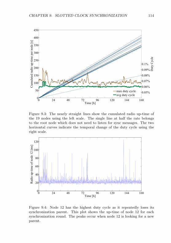
CHAPTER 9. SLOTTED CLOCK SYNCHRONIZATION 114
0 24 48 72 96 120 144 1680
50
100
150
200
250
300
350
400
450
Time [h]
Cum
ulat
ed ra
dio
up-ti
me
per n
ode
[s]
0.05%
0.06%
0.07%
0.08%
0.09%
0.1%
Dut
y C
ycle
max duty cycleavg duty cycle
Figure 9.3: The nearly straight lines show the cumulated radio up-time ofthe 19 nodes using the left scale. The single line at half the rate belongsto the root node which does not need to listen for sync messages. The twohorizontal curves indicate the temporal change of the duty cycle using theright scale.
0 24 48 72 96 120 144 1680
20
40
60
80
100
120
Time [h]
Rad
io u
p-tim
e of
nod
e 12
[ms]
Figure 9.4: Node 12 has the highest duty cycle as it repeatedly loses itssynchronization parent. This plot shows the up-time of node 12 for eachsynchronization round. The peaks occur when node 12 is looking for a newparent.

10Low-Power Signaling
As a case study for slotted programming, this chapter describes the construc-tion of an alarm system in which any node or any subset of nodes can alarmall other nodes. The reliability of such a system is often guaranteed throughthe following two phases: In the first phase, the nodes are awaken throughan energy efficient wake-up mechanism. Once the nodes are awake, the veri-fication phase kicks in to rule out false alarms, authenticate the originator(s)of the alarm, and perform other security relevant tasks before relaying thealarm to the upper layer. Whereas this second phase may be costly in termsof energy, this is no issue for most scenarios where alarms can be assumed tooccur rarely. On the contrary, the wake-up functionality should be as powerefficient as possible because it must be constantly available. In addition, thewake-up should provoke as few false alarms as possible in order not to triggerthe second phase unnecessarily.
In this chapter, we only consider the wake-up phase and present a noveltechnique to reliably transmit a wake-up signal. Our idea is the following:Instead of transmitting ordinary messages to announce an alarm, a nodesends an unmodulated wave at a constant frequency. With this approach, wesolve two problems at one fell swoop. Firstly, several nodes may announcean alarm at the same time without causing interference. This holds becausethe superposition of several waves of the same frequency is received as awave of the given frequency. Secondly, we can build tight schedules for thesignal propagation. Previously, this was possible only with RSSI sniffs whichtend to give many false alarms when used outdoors. Both, the interferenceresistance and the tight scheduling lay the basis for our energy efficient wake-up phase. We propose a pipelined dissemination of the alarm signal such thatthe dissemination delay is minimized. For each execution of the pipeline, thenodes need to power the radio module for a total of 14ms in the currentimplementation. Thus, the overall energy consumption of the wake-up phase

CHAPTER 10. LOW-POWER SIGNALING 116
depends on the frequency at which these pipelines are scheduled. E.g. havinga dissemination every 30 seconds causes a radio duty cycle of only 0.04%, butalso delays the delivery of a potential alarm by up to 30 seconds. Clearly,this parameter is application specific.
A special configuration of the radio module is required to generate thedesired waves. As the radio also needs to support standard messages, theapplication must ensure the required radio configuration at any time. Thisguarantee comes nearly for free with a slotted application where the tasks,and therefore also the conflicting configurations, are temporally decoupled.
10.1 Pipelining
The end-to-end delay of such an alarm can be minimized by pipelining thetransmissions of the nodes. But as any node of the network may initiatean alarm, the pipelining would need to provide an any-to-all support. Toovercome this complex task, we reduce the problem to the following twopipelinings: any-to-root and root-to-all, where the root is a dedicated node,e.g. a sink node or the node leading the clock synchronization. This resultsin a 2-phase approach, where the initiating node first signals the root nodeabout the alarm (any-to-root) and the root then signals the alarm to theentire network (root-to-all).
The classic approach to both pipelinings is to build a BFS tree from theroot node. When sending messages to transmit the alarm, however, carehas to be taken to not cause interference. In the root-to-all phase, the rootnode first broadcasts its message to all its direct children in the tree. Uponreceiving the message, the children should be coordinated to not forward themessage at the same instant. The same problem exists in the any-to-rootphase, where several children of a parent may wish to signal an alarm, oran alarm is propagated on several branches of the BFS tree. This issue canbe solved by either using a global schedule or by applying randomizationtechniques. But both solutions are not satisfactory as they increase the end-to-end delay. Furthermore, the overhead to maintain a global schedule maybe considerable.
10.2 Signaling of Binary States
As we are interested only in binary states (e.g. alarm ON, alarm OFF), amuch simpler solution is possible. For instance, the value ON may be encodedby sending a message and the value OFF by being quiet. In the any-to-rootcase, each parent only needs to detect whether any of its children sends amessage, and depending on the outcome, send a message itself or not. Todo so, the parent only needs to detect the activity on the radio channel,e.g. through an RSSI sniff, eliminating the interference problem. Therefore,
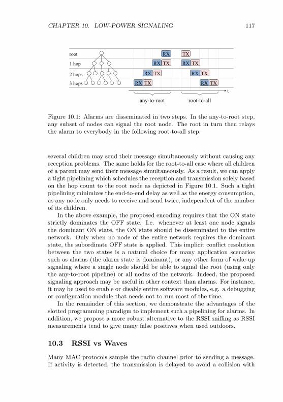
CHAPTER 10. LOW-POWER SIGNALING 117
root
1 hop
2 hops
3 hops RX TX
RX TX
RX TX
RX TX
RX TX
RX TX
RX TX
t
any-to-root root-to-all
Figure 10.1: Alarms are disseminated in two steps. In the any-to-root step,any subset of nodes can signal the root node. The root in turn then relaysthe alarm to everybody in the following root-to-all step.
several children may send their message simultaneously without causing anyreception problems. The same holds for the root-to-all case where all childrenof a parent may send their message simultaneously. As a result, we can applya tight pipelining which schedules the reception and transmission solely basedon the hop count to the root node as depicted in Figure 10.1. Such a tightpipelining minimizes the end-to-end delay as well as the energy consumption,as any node only needs to receive and send twice, independent of the numberof its children.
In the above example, the proposed encoding requires that the ON statestrictly dominates the OFF state. I.e. whenever at least one node signalsthe dominant ON state, the ON state should be disseminated to the entirenetwork. Only when no node of the entire network requires the dominantstate, the subordinate OFF state is applied. This implicit conflict resolutionbetween the two states is a natural choice for many application scenariossuch as alarms (the alarm state is dominant), or any other form of wake-upsignaling where a single node should be able to signal the root (using onlythe any-to-root pipeline) or all nodes of the network. Indeed, the proposedsignaling approach may be useful in other context than alarms. For instance,it may be used to enable or disable entire software modules, e.g. a debuggingor configuration module that needs not to run most of the time.
In the remainder of this section, we demonstrate the advantages of theslotted programming paradigm to implement such a pipelining for alarms. Inaddition, we propose a more robust alternative to the RSSI sniffing as RSSImeasurements tend to give many false positives when used outdoors.
10.3 RSSI vs Waves
Many MAC protocols sample the radio channel prior to sending a message.If activity is detected, the transmission is delayed to avoid a collision with

CHAPTER 10. LOW-POWER SIGNALING 118
the ongoing transmission. This sampling is called clear channel assessment(CCA) and is often performed by an RSSI module on the radio chip whichindicates the received signal strength. If the value is above a given threshold,the channel is assumed to be occupied. We propose to use exactly this toolto circumvent interference problems while signaling an alarm. Indeed, theapproach works surprisingly well - as long as all nodes are deployed indoors.But as soon as we placed nodes on the roof of our building, the RSSI modulestarted to intercept foreign signals, leading to roughly 30% false positives,i.e. the RSSI module indicates activity on the channel even though none ofthe nodes is sending. Whereas this degrades the performance but may stillbe acceptable for some MAC protocols, the state signaling task requires afar more reliable solution as false alarms or unnecessary wake-ups can becostly. Ideally, an alternative approach still allows for a tight pipelining ofthe transmissions without causing interference.
In the presented RSSI approach, the transmitters send arbitrary messagesas the receiver only looks for activity on the radio channel. To reduce thenumber of false positives during silent phases, we propose to slightly changethe scheme and require all transmitters to send the exactly same messagewhich needs to be decoded by the receiver. Consequently, the probabilityto decode the expected message even though no node is transmitting dropsexponentially. Whereas this method resolves the problem of false positives, itis prone to interference, as all transmitters would need to be highly synchro-nized to send each bit of the message at exactly the same time. Therefore,we carefully choose the message such that the resulting radio signal is an un-modulated wave of constant frequency. This solves the interference problemat one fell swoop as the mixture of several waves of the same frequency isreceived as a wave signal of the given frequency. But whereas MIMO andSIMO radios make explicit use of this property to amplify the radio signal ina certain location, we have no influence on the phase at which the distributedtransmitters send. As a result, some receivers may get an attenuated signal.Fortunately, the probability for a complete attenuation is extremely low, andour experiments indicate that the number of false negatives is in the range of0.1% and comparable to the RSSI approach (See Table 10.1). In summary,the proposed approach encodes the dominant state by sending an unmodu-lated signal of constant frequency, and the subordinate state is encoded bybeing quiet.
The desired radio wave can be generated easily with our XE1205 radiomodule as it applies an FSK modulation. In this modulation technique, abinary ’0’ is encoded by sending a wave at frequency f0 and a binary ’1’ is en-coded by sending a wave at frequency f1. For sending and receiving standardmessages, the radio runs in a buffered mode utilizing a bit synchronizer andpattern recognition block. When generating or sampling waves, we switch toa continuous mode through which we can send raw data or directly access

CHAPTER 10. LOW-POWER SIGNALING 119
wave
RSSI
enable
radio
enable
radio
2ms 5ms 8.5ms
sample wave send wave
2ms 5ms
send RSSI packet sample RSSI
Figure 10.2: When a node is scheduled within the pipeline, it enables its ra-dio, samples the RSSI or the wave, and depending on the outcome, transmitsitself an RSSI packet or a wave, respectively.
the received signal. Please refer to Chapter 10.5.1 for a description of theused hardware and more details on its usage. Also note that the generationof these waves may be harder to obtain on packet-based radios or on radiosthat apply an encoding such as Manchester or NRZI.
10.4 Slotted Signaling
In the remainder of this section we outline the implementation of a testapplication to compare the RSSI and the wave approach for the signalingtask. Similar to the first case study, our focus is on the software architecture,rather than the implementation details.
Signaling Module The task of the signaling module is to run an any-to-root sweep to detect requests to change a state, followed by a root-to-allsweep to disseminate a potential request to the entire network. Both sweepsare implemented in a pipelined fashion as described in Chapter 10.1. As thetimings for the RSSI as well as the wave approach are similar, we can use thesame pipelining for the comparison, see Figure 10.2. The time to enable theradio is approximately 2ms and the time to send an RSSI message is 4.5ms.The RSSI value is sampled three times in a row, indicating a signal only if allthree measurements show high activity on the radio channel. We hoped toreduce the number of false positives with this approach, but the experimentsdid not show a significant improvement compared to a single RSSI sniff,indicating a high correlation of the RSSI measurements. The sampling timefor the wave is set to 5ms yielding 378 samples, and the transmission time fora wave is set to a total of 8.5ms to account for synchronization fluctuations.
The signaling module allocates itself a time slot of 1 second. The first500ms is reserved for the any-to-root pipeline and the second 500ms for theroot-to-all pipeline. As the overlap of the sender and receiver is only 7ms ineach pipeline step, the depth of the pipelines may be up to 60 hops (leaving

CHAPTER 10. LOW-POWER SIGNALING 120
some time gap at the beginning and the end of the time slot). Thus, thecurrent settings theoretically allow for large networks with a diameter up to120 hops if the root node is chosen in the center.
Whenever startSlot() is called, the signaling module retrieves the node’shop-count to the root from the clock synchronization module and determinesits start-time in the any-to-root and the root-to-all pipeline. An adaptation ofthis hop-count is however necessary, as the links used by the synchronizationtree may be unidirectional. This adaptation is implemented by a simpleonline search that is launched whenever the root-to-all sweep does not reflecta request sent on the any-to-root sweep.
Energy Cost of Signaling The energy cost of the signaling is dominatedby the energy used by the radio module for sampling and sending. In manyapplication scenarios, a signal will only be disseminated rarely on specialevents. During the silent periods, a node needs to enable its radio once forthe any-to-root and once for the root-to-all pipeline, requiring an up-time of14ms. In the event of a signaling, a node may enable its radio up to 31msto participate in the two pipelines. The overall energy cost for the signalingdepends on the frequency at which the signaling module is scheduled andhow often signals are disseminated.
10.5 Test Application
The integration of the signaling module into an application, in our case a testapplication to compare the RSSI and the wave signaling, is straight forward.All we need to do is to assign time slots to each module such as to obtaina non-overlapping schedule. In our test application, we utilize the followingsoftware modules:
• Clock synchronization module
• RSSI signaling module
• Wave signaling module
• Remote control module
• Feedback composition module
The remote control module is used for collecting the logs of an ongoingexperiment and for debugging the application. The module supports multi-hop message forwarding to deliver log messages at a base station such that wecan track the progress of an ongoing experiment. In addition, it can also routecommand messages from the base station to any given node in the network,

CHAPTER 10. LOW-POWER SIGNALING 121
C
S
RC W R W R W R W R W R W R W R W R F
9 10 11 12 13 14 15 16
32 64
C
S
RC W R W R W R W R W R W R W R W R
17 18 19
64 96
C
S
RC W R W R W R W R W R W R W R W R F
random subset
96 128
C
S
RC W R W R W R W R W R W R W R W R
1 2 3 4 5 6 7 8
0 32
Figure 10.3: The test application to compare the wave signaling and the RSSIsignaling allocates a total of 74 time slots within the scheduling window of128 seconds. The following abbreviations are used for the modules: CS -Clock Synchronization, RC - Remote Control, F - Feedback composition, W- wave signaling, and R - RSSI signaling. The numbers above the time slotsindicate the ID of the node which triggers an alarm.

CHAPTER 10. LOW-POWER SIGNALING 122
Figure 10.4: The nodes 5, 15, 16, 17, 18, and 19 are placed outside thebuilding and are powered by battery. Whereas the nodes 15, 18, and 19are on the roof, the nodes 5, 16, and 17 are placed on the facade along thefour floors to the roof to establish a radio connection with the nodes onthe roof. Node 1 is configured to be the root for the clock synchronizationand the signaling. The dashed lines show an instance of the dynamic clocksynchronization tree.
which was convenient to debug the application in its initial phase. Thefeedback composition module collects and preprocesses the local data fromthe experiment and feeds the remote control module with the log messages.Both of these modules support our experiments, but they do not influencethe synchronization and signaling tasks in any way as they are temporallydecoupled. Therefore, they could be removed from the application withoutconsequences for the other modules.
The test application uses an allocation window of 128 seconds withinwhich it schedules its modules, see Figure 10.3. The clock synchronizationmodule is scheduled every 32 seconds, followed by the remote control modulethat gathers the log messages. Every 64 seconds, the feedback compositionmodule prepares the log messages which are sent in the forthcoming remotecontrol time slot. The RSSI signaling module and the wave signaling moduleare assigned a total of 64 time slots within the remaining allocation windowto test as many signaling rounds as possible. The two approaches are testedin an alternating fashion such that they undergo similar external influences.

CHAPTER 10. LOW-POWER SIGNALING 123
10.5.1 Deployment and Experiment Setup
We performed our experiments with the TinyNode 584 from ShockfishSA [87]. This sensor node features an MSP430 CPU with 10kB RAM and48kB program space and works with the Xemics XE1205 radio which appliesan FSK modulation. For receiving data packets, the radio is configured ina buffered mode with a built-in bit synchronizer and a pattern detector. Asthe bit synchronizer requires at least some bit transitions every now and thento operate correctly, we cannot use the buffered mode for detecting alarms,as they consist of a wave of a given frequency. We therefore use the con-tinuous mode of the radio which skips the bit synchronization and patternrecognition and outputs the raw bit sequence on a data pin. Our applicationsamples this stream during 5ms to obtain the described sampling. Whereaswe could transmit waves in the buffered mode by sending a message withevery bit set to 1 (or 0), this requires quite some modification on the radiostack. In continuous mode, the transmission of a wave is straight forward, asthe radio sends the pattern that is applied to a given pin. Keeping the pinat 1 (or 0) results in the desired wave.
For our experiment, we have deployed a total of 19 nodes, 6 of them areoutside the building, see Figure 10.4. Node 1 acts as base station and asroot for the clock synchronization. The goal of the experiment is to testthe reliability of the proposed wave signaling and compare it to the RSSIapproach. In particular, we are interested in the following two errors: A“false negative” signaling happens when a node fails to detect a signal sentby a neighboring node. This type of error is especially undesirable in alarmsystems where the system should immediately react to a new situation. A“false positive” signaling occurs when a node detects a signal even thoughno node is transmitting. This fault is often called a “false alarm”.
To test for these errors, the following scenario is run through in eachwindow of the slot scheduler, Figure 10.3 depicts the setup.
• Exactly one node triggers an alarm in the first 38 time slots. Eachnode is assigned a time slot pair (consisting of a time slot for the wavesignaling and one for the RSSI signaling) during which it triggers analarm. This is done by sending a wave or an message, respectively, atthe assigned time within the any-to-root pipeline.
• None of the nodes triggers an alarm during the following 16 time slots.
• A randomly chosen subset of the nodes triggers an alarm in the remain-ing 5 time slot pairs. This last test case is used to explicitly examinethe decoding resistance when several nodes signal synchronously.
For each of these time slots, we decide whether the signaling was successfulor not. As the signaling module described in Chapter 10.4 performs an any-

CHAPTER 10. LOW-POWER SIGNALING 124
0 24 48 72 96 120 144 1680
2000
4000
6000
8000
10000
12000C
umul
ated
# o
f RSS
I fal
se a
larm
s
Time [h]
10%
20%
30%
40%
50%
% o
f fal
se a
larm
s
Figure 10.5: The solid line shows the cumulated number of false positiveswhen using RSSI sniffs (left scale). The bumpy curve depicts the temporalvariability of the error probability (using the right scale).
to-root sweep followed by a root-to-all sweep, all nodes are supposed to havethe same state at the end of the signaling time slot. Therefore, if one orseveral nodes fail to detect the signal in the root-to-all sweep, we count thetime slot as false negative. Similarly, if one or several nodes detect a signal inone of the 16 silent time slots, we count the time slot as false positive. Pleasenote that we test the overall signaling procedure rather than each individualsignal decoding as the latter is prone to report subsequent errors.
10.5.2 Results
We have run the above experiment for 168 hours. During this time, theschedule of Figure 10.3 was repeated 4725 times, generating 113400 roundsin which at least one node triggered an alarm and 37800 silent rounds withoutalarm. Table 10.1 summarizes the overall outcome of the experiment. Onaverage, the RSSI had false alarms in 31% of the silent rounds, compared toonly 0.8% of the wave approach. The probability for a dropped alarm (falsenegative) is comparable for both the wave and RSSI approach.
Figure 10.5 depicts the cumulated number of RSSI false alarms, and thehorizontal curve shows how the error probability changes over time. WhereasRSSI suffers from false alarms in 31% on average, the curve shows that theerror probability is sometimes as low as 10% for an extended period of time.

CHAPTER 10. LOW-POWER SIGNALING 125
Table 10.1: Performance of the wave and the RSSI signaling.Wave RSSI Numbersignaling signaling of tests
False positives 304 (0.8%) 11815 (31%) 37800
False negatives 94 (0.08%) 132 (0.11%) 113400
24 48 72 96 120 144 1680
50
100
150
200
250
300
350
Cum
ulat
ed n
umbe
r of e
rror
s
Time [h]
wave false positiveswave false negativesRSSI false negatives
Figure 10.6: Cumulated number of errors without the RSSI false positives.Please note that errors tend to happen in bursts.
This fact can also be observed on the cumulative curve, where the slopeflattens temporarily during the early afternoon of the first and last day ofthe experiment. (Please note that all plots start at midnight.) We belivethat this improvement could be related to the weather, as only the first andlast day of the experiment was sunny.
In contrast to the RSSI approach, the wave signaling has much less falsealarms. Figure 10.6 shows the temporal developing of the false positives andfalse negatives of the wave signaling as well as the false negatives of the RSSIapproach. Please note that most errors come in bursts, indicating a temporalcorrelation between successive samplings of the same kind. So far, we haveno explanation for these errors.
When decoding a wave transmission, a node samples the radio channelduring 5ms resulting in 378 samplings. As our radio module applies an

CHAPTER 10. LOW-POWER SIGNALING 126
70% 75% 80% 85% 90% 95% 100%
101
102
103
104
105
106
Num
ber o
f rec
eive
d si
gnal
ings
Wave sampling percentage
Figure 10.7: For each decoded wave, the nodes remembered the percentageof correct bits. This plot shows that a large majority of the alarms hasall or nearly all bits correctly, and that the probability for errors decreasesexponentially.
FSK decoding, each sample indicates which of the two frequencies is morelikely. If no wave is being transmitted, the radio module decodes whitenoise indicating either frequency with a probability of 50%. However, if aneighboring node transmits a wave at frequency fx, the radio module reportsall samples to be at frequency fx. The node counts the number of sampleswith the expected frequency and indicates an alarm only if this number isabove a given threshold. In our implementation, at least 70% of the samplesmust indicate the expected frequency.
Figure 10.7 shows the number of received alarms as a function of the de-coding percentage. For over 63% of the decoded alarms, all samples indicatedthe expected frequency. In 99.9% of the detected alarms, at least 75% of thesamples indicated the expected frequency. Thus, setting 70% as thresholdseems reasonable.

11Conclusion
In the second part of this thesis, we proposed a novel signaling technique tobuild energy efficient alarm systems. Our wave based approach is resilient tointerference, allows for a tight pipeline scheduling without unnecessary hop-by-hop delay, is energy efficient at a duty cycle of less than 0.1%, and causesfew false alarms even when used outdoors. We believe that our signalingscheme is a valuable alternative to traditional message based approacheswhich need to handle interference. For instance, low power listening schemesassume that messages are transmitted only sporadically such that messagecollisions are rare. In an alarming scenario, however, a possibly large subsetof nodes may detect an abnormal state and trigger an alarm at the sameinstant. While message-based approaches are burdened with the overheadto avoid interference, the proposed wave signaling is specifically designed tosupport simultaneous alarms, allowing for a better energy efficiency.
The implementation of such an alarm system is rather involved. Firstly,the transmission and reception of waves requires a special configuration ofthe radio module which does not support data messages. Thus, the appli-cation must ensure a suitable configuration at all times. Secondly, the tightpipelining for the alarm dissemination requires each node to enable its radioexactly at the assigned time. If this operation is delayed by another task run-ning on the node, a potential alarm may not be detected. With the slottedprogramming approach, both issues are solved with the temporal separationof the modules. In addition, the modularity of the software components al-lowed us to setup a rather complex application to compare the RSSI and thewave signaling with little effort.
Overall, we feel that the slotted programming approach greatly sup-ported our work and we believe the slotted programming paradigm to bea valuable tool for developing sensor network applications in general. Butthe advantages are not only in the facilitated software development. Just as
CHAPTER 11. CONCLUSION 128
important are the modularity and temporal separation of the different taskswhich allow for a predictable execution of the application. This predictabilityis also a basic requirement to build systems for which certain properties canbe guaranteed. In fact, the development of provably correct software is veryhard in general. The core difficulty lies in the fact that it is hard to comparethe application (written in a programming language) and the specification(written in a descriptive language). The slotted programming paradigmcannot solve this problem, but it shortens the gap between the two worldsby reducing the complexity of the software implementation, rendering thecomparison easier. Most importantly, the slotted programming achievesthis by temporally decoupling independent tasks such that the differentcomponents can be checked separately. In addition, the temporal decouplingrenders unnecessary many asynchronous code blocks as timely executionis ensured implicitly by the slotted execution model. For instance, theapplication to evaluate the alarming system of Chapter 10 requires noasynchronous code block except for the system events. Such synchronouscode is much easier to analyze as there are much fewer execution patternsto be considered and the simplified code itself reduces the risk of bugs.
Wireless sensor networks will gain more attention in the near future asengineers in various fields become aware of the novel technology and its ca-pabilities. But as wireless ad hoc networking is still in its infancy it needsto go a long path to unfold its full potential. Towards this goal, the technol-ogy first needs to gain acceptance by proving reliability and practicability.Therefore, we not only need to build appropriate hardware, but also providesuitable tools to efficiently develop the corresponding software. We believethat it is important to facilitate the software development process for wire-less sensor networks such that programming is not only easier, but also morebug-resistant. Within this context, the slotted programming paradigm isonly a small piece of a huge puzzle through which we hope to contribute toa more efficient development of energy efficient software for sensor networks.
Bibliography
[1] H. Abrach, S. Bhatti, J. Carlson, H. Dai, J. Rose, A. Sheth, B. Shucker,J. Deng, and R. Han. MANTIS: System Support for Multimodal Net-works of In-Situ Sensors. In WSNA, 2003.
[2] I. Abraham, D. Dolev, and D. Malkhi. LLS: a Locality Aware LocationService for Mobile Ad Hoc Networks. In DIAL-M-POMC, 2004.
[3] I. Abraham, C. Gavoille, A. Goldberg, and D. Malkhi. Routing inNetworks with Low Doubling Dimension. In ICDCS, 2006.
[4] J. Aspnes, D. K. Goldenberg, and Y. R. Yang. On the ComputationalComplexity of Sensor Network Localization. In ALGOSENSORS, 2004.
[5] C. Avin and G. Ercal. On the Cover Time and Mixing Time of RandomGeometric Graphs. Theoretical Computer Science, 380(1-2):2–22, 2007.
[6] C. Avin and B. Krishnamachari. The Power of Choice in RandomWalks: An Empirical Study. In MSWiM, 2006.
[7] B. Awerbuch and D. Peleg. Sparse Partitions (Extended Abstract). InFOCS, 1990.
[8] B. Awerbuch and D. Peleg. Online Tracking of Mobile Users. Journalof the ACM, 42(5):1021–1058, 1995.
[9] G. Barnes and U. Feige. Short Random Walks on Graphs. In STOC,1993.
[10] S. Basagni, I. Chlamtac, V. R. Syrotiuk, and B. A. Woodward. A Dis-tance Routing Effect Algorithm for Mobility (DREAM). In MobiCom,1998.
[11] L. Blazevic, J.-Y. Le Boudec, and S. Giordano. A Location-BasedRouting Method for Mobile Ad Hoc Networks. IEEE Trans. Mob.Comput., 4(2):97–110, 2005.

BIBLIOGRAPHY 130
[12] P. Bose and P. Morin. An Improved Algorithm for Subdivision Traver-sal without Extra Storage. In ISAAC, 2000.
[13] P. Bose, P. Morin, I. Stojmenovic, and J. Urrutia. Routing With Guar-anteed Delivery in Ad Hoc Wireless Networks. In DIAL-M, 1999.
[14] H. Breu and D. G. Kirkpatrick. Unit Disk Graph Recognition is NP-hard. Computational Geometry, Theory and Applications, 9(1-2):3–24,1998.
[15] N. Brouwers, P. Corke, and K. Langendoen. A Java Compatible VirtualMachine for Wireless Sensor Nodes. In SenSys, 2008.
[16] J. Bruck, J. Gao, and A. A. Jiang. Localization and Routing in SensorNetworks by Local Angle Information. In MobiHoc, 2005.
[17] M. Buettner, G. V. Yee, E. Anderson, and R. Han. X-MAC: A ShortPreamble MAC Protocol for Duty-Cycled Wireless Sensor Networks.In SenSys, 2006.
[18] N. Burri, P. von Rickenbach, and R. Wattenhofer. Dozer: Ultra-LowPower Data Gathering in Sensor Networks. In IPSN, April 2007.
[19] H. T.-H. Chan, A. Gupta, B. M. Maggs, and S. Zhou. On HierarchicalRouting in Doubling Metrics. In SODA, 2005.
[20] A. K. Chandra, P. Raghavan, W. L. Ruzzo, and R. Smolensky. TheElectrical Resistance of a Graph Captures its Commute and CoverTimes. In STOC, 1989.
[21] J. Chen, A. Jiang, I. A. Kanj, G. Xia, and F. Zhang. Separability andTopology Control of Quasi Unit Disk Graphs. In INFOCOM, 2007.
[22] M. B. Chen, C. Gotsman, and C. Wormser. Distributed Computationof Virtual Coordinates. In SCG, 2007.
[23] N. Cooprider, W. Archer, E. Eide, D. Gay, and J. Regehr. EfficientMemory Safety for TinyOS. In SenSys, 2007.
[24] S. M. Das, H. Pucha, and Y. C. Hu. Performance Comparison of Scal-able Location Services for Geographic Ad Hoc Routing. In INFOCOM,2005.
[25] S. Datta, I. Stojmenovic, and J. Wu. Internal Node and Shortcut BasedRouting with Guaranteed Delivery in Wireless Networks. ICDCSW,5(2):169–178, 2002.

BIBLIOGRAPHY 131
[26] F. de Rango, M. Gerla, B. Zhou, and S. Marano. Geo-LANMAR Rout-ing: Asymptotic Analysis of a Scalable Routing Scheme with GroupMotion Support. In BROADNETS, 2005.
[27] S. Dobrev, J. Jansson, K. Sadakane, and W.-K. Sung. Finding ShortRight-Hand-on-the-Wall Walks in Graphs. In SIROCCO, 2005.
[28] A. Dunkels, B. Gronvall, and T. Voigt. Contiki – a Lightweight andFlexible Operating System for Tiny Networked Sensors. In Emnets,2004.
[29] A. Dunkels, O. Schmidt, T. Voigt, and M. Ali. Protothreads: Simpli-fying Event-Driven Programming of Memory-Constrained EmbeddedSystems. In SenSys, 2006.
[30] S. Durocher, D. Kirkpatrick, and L. Narayanan. On Routing withGuaranteed Delivery in Three-Dimensional Ad Hoc Wireless Networks.In ICDCN, 2008.
[31] M. Dyer, J. Beutel, and L. Thiele. S-XTC: A Signal-Strength BasedTopology Control Algorithm for Seonsor Networks. In ISADS, 2007.
[32] A. El-Hoiydi and J.-D. Decotignie. WiseMAC: An Ultra Low PowerMAC Protocol for the Downlink of Infrastructure Wireless Sensor Net-works. In Computers and Communications, 2004.
[33] D. Eppstein and M. T. Goodrich. Succinct Greedy Graph Drawing inthe Hyperbolic Plane. In GD, 2008.
[34] J. Eriksson, M. Faloutsos, and S. Krishnamurthy. Scalable Ad HocRouting: The Case for Dynamic Addressing. In INFOCOM, 2004.
[35] A. Eswaran, A. Rowe, and R. Rajkumar. Nano-RK: An Energy-AwareResource-Centric RTOS for Sensor Networks. In RTSS, 2005.
[36] Q. Fang, J. Gao, and L. J. Guibas. Locating and Bypassing RoutingHoles in Sensor Networks. In INFOCOM, 2004.
[37] Q. Fang, J. Gao, L. J. Guibas, V. Silva, and L. Zhang. GLIDER:Gradient Landmark-Based Distributed Routing for Sensor Networks.In INFOCOM, 2005.
[38] U. Feige. A Tight Upper Bound on the Cover Time for Random Walkson Graphs. Random Struct. Algorithms, 6(1):51–54, 1995.
[39] R. Flury. Sinalgo - Simulator for Network Algorithms. http://
sinalgo.sourceforge.net, May 2009.

BIBLIOGRAPHY 132
[40] R. Flury, S. Pemmaraju, and R. Wattenhofer. Greedy Routing withBounded Stretch. In INFOCOM, 2009.
[41] R. Fonseca, R. Fonseca, S. Ratnasamy, S. Ratnasamy, D. Culler,D. Culler, S. Shenker, S. Shenker, I. Stoica, and I. Stoica. BeaconVector Routing: Scalable Point-To-Point Routing in Wireless Sensor-nets. In NSDI, 2005.
[42] C. Gavoille and M. Gengler. Space-Efficiency for Routing Schemes ofStretch Factor Three. Journal of Parallel and Distributed Computing,61(5):679–687, 2001.
[43] C. Gotsman and Y. Koren. Distributed Graph Layout for Sensor Net-works. In GD, 2004.
[44] A. Grilo, M. Macedo, and M. Nunes. An Energy-Efficient Low-LatencyMulti-sink MAC Protocol for Alarm-Driven Wireless Sensor Networks.LNCS, 2007.
[45] M. Grossglauser and M. Vetterli. Locating Mobile Nodes WithEASE: Learning Efficient Routes From Encounter Histories Alone.IEEE/ACM Transactions on Networking, 14(3):457–469, 2006.
[46] L. Gu and J. A. Stankovic. t-kernel: Providing Reliable OS Supportto Wireless Sensor Networks. In SenSys, 2006.
[47] A. Gupta, A. Kumar, and R. Rastogi. Traveling with a Pez Dis-penser (or, Routing Issues in MPLS). SIAM Journal on Computing,34(2):453–474, 2004.
[48] C.-C. Han, R. Kumar, R. Shea, E. Kohler, and M. Srivastava. ADynamic Operating System for Sensor Nodes. In MobiSys, 2005.
[49] T. Harbaum. NanoVM. http://www.harbaum.org/till/nanovm,March 2009.
[50] T. He, C. Huang, B. M. Blum, J. A. Stankovic, and T. Abdelzaher.Range-Free Localization Schemes for Large Scale Sensor Networks. InMobiCom, 2003.
[51] J. W. Hui and D. E. Culler. IP is Dead, Long Live IP for WirelessSensor Networks. In SenSys, 2008.
[52] R. Kleinberg. Geographic Routing Using Hyperbolic Space. In INFO-COM, 2007.
[53] G. Konjevod, A. W. Richa, and D. Xia. Optimal-Stretch Name-Independent Compact Routing in Doubling Metrics. In PODC, 2006.
BIBLIOGRAPHY 133
[54] L. Kou, G. Markowsky, and L. Berman. A Fast Algorithm for SteinerTrees. Acta Informatica, 15:141–145, 1981.
[55] A. Kroeller, D. Pfisterer, C. Buschmann, S. P. Fekete, and S. Fischer.Shawn: A New Approach to Simulating Wireless Sensor Networks. InDASD, 2005.
[56] A. Kroller, S. P. Fekete, D. Pfisterer, and S. Fischer. DeterministicBoundary Recognition and Topology Extraction for Large Sensor Net-works. In SODA, 2006.
[57] F. Kuhn, T. Moscibroda, T. Nieberg, and R. Wattenhofer. FastDeterministic Distributed Maximal Independent Set Computation onGrowth-Bounded Graphs. In DISC, September 2005.
[58] F. Kuhn, T. Moscibroda, and R. Wattenhofer. What Cannot Be Com-puted Locally! In PODC, July 2004.
[59] F. Kuhn, R. Wattenhofer, Y. Zhang, and A. Zollinger. Geometric Ad-Hoc Routing: of Theory and Practice. In PODC, 2003.
[60] F. Kuhn, R. Wattenhofer, and A. Zollinger. Asymptotically OptimalGeometric Mobile Ad Hoc Routing. In DIAL-M, 2002.
[61] J.-Y. Le Boudec and M. Vojnovic. Perfect Simulations and Stationarityof a Class of Mobility Models. In INFOCOM, 2005.
[62] P. Levis, N. Lee, M. Welsh, and D. Culler. TOSSIM: Accurate andScalable Simulation of Entire TinyOS Applications. In SenSys, 2003.
[63] J. Li, J. Jannotti, D. S. J. D. Couto, D. R. Karger, and R. Morris. AScalable Location Service for Geographic Ad Hoc Routing. In Mobi-Com, 2000.
[64] M. Li, W.-C. Lee, and A. Sivasubramaniam. Efficient Peer-to-PeerInformation Sharing over Mobile Ad Hoc Networks. In MobEA, 2004.
[65] N. Linial, E. London, and Y. Rabinovich. The Geometry of Graphs andSome of its Algorithmic Applications. Combinatorica, 15(2):215–245,1995.
[66] R. J. Lipton and R. E. Tarjan. A Separator Theorem for Planar Graphs.SIAM Journal on Computing, 36(2):177–189, 1979.
[67] K. Lorincz, B. Chen, J. Waterman, G. Werner-Allen, and M. Welsh.Resource Aware Programming in the Pixie OS. In SenSys, 2008.
BIBLIOGRAPHY 134
[68] L. Lovasz. Random Walks on Graphs: A Survey. Combinatorics,2:353–398, 1996.
[69] M. Luby. A Simple Parallel Algorithm for the Maximal IndependentSet Problem. SIAM Journal on Computing, 15:1036–1053, 1986.
[70] M. Maroti, B. Kusy, G. Simon, and A. Ledeczi. The Flooding TimeSynchronization Protocol. In SenSys, 2004.
[71] W. P. McCartney and N. Sridhar. Abstractions for Safe ConcurrentProgramming in Networked Embedded Systems. In SenSys, 2006.
[72] A. Moitra and T. Leighton. Some Results on Greedy Embeddings inMetric Spaces. In FOCS, 2008.
[73] D. Moore, J. Leonard, D. Rus, and S. Teller. Robust DistributedNetwork Localization With Noisy Range Measurements. In SenSys,2004.
[74] ns-2. http://nsnam.isi.edu/nsnam/index.php, May 2009.
[75] C. H. Papadimitriou and D. Ratajczak. On a Conjecture Related toGeometric Routing. Theoretical Computer Science, 344(1):3–14, 2005.
[76] D. Peleg and E. Upfal. A Trade-Off between Space and Efficiency forRouting Tables. J. ACM, 36(3):510–530, 1989.
[77] S. V. Pemmaraju and I. A. Pirwani. Good Quality Virtual Realizationof Unit Ball Graphs. In ESA, 2007.
[78] M. Penrose. The Longest Edge of the Random Minimal Spanning Tree.The Annals of Applied Probability, 7(2):340–361, 1997.
[79] J. Polastre, J. Hill, and D. Culler. Versatile Low Power Media Accessfor Wireless Sensor Networks. In SenSys, 2004.
[80] A. Rao, C. Papadimitriou, S. Shenker, and I. Stoica. Geographic Rout-ing Without Location Information. In MobiCom, 2003.
[81] S. Ratnasamy, B. Karp, L. Yin, F. Yu, D. Estrin, R. Govindan, andS. Shenker. GHT: a Geographic Hash Table for Data-Centric Storage.In WSNA, 2002.
[82] A. L. Rosenberg and L. S. Heath. Graph Separators, with Applications.Springer: Frontiers in Computer Science, 2000.
[83] P. Santi. Topology Control in Wireless Ad Hoc and Sensor Networks.ACM Computing Surveys, 2005.

BIBLIOGRAPHY 135
[84] S. Schmid and R. Wattenhofer. Algorithmic Models for Sensor Net-works. In WPDRTS, April 2006.
[85] Sentilla. Sentilla Perk. http://sentilla.com/perk, May 2009.
[86] Y. Shang and W. Ruml. Improved MDS-based localization. In INFO-COM, 2004.
[87] Shockfish SA. TinyNode. http://www.tinynode.com, November 2008.
[88] A. Slivkins. Distance Estimation and Object Location via Rings ofNeighbors. In PODC, 2005.
[89] A. Smith, H. Balakrishnan, M. Goraczko, and N. B. Priyantha. Track-ing Moving Devices with the Cricket Location System. In MobiSys,2004.
[90] Y. Sun, O. Gurewitz, and D. B. Johnson. RI-MAC: a Receiver-InitiatedAsynchronous Duty Cycle MAC Protocol for Dynamic Traffic Loads inWireless Sensor Networks. In SenSys, 2008.
[91] K. Talwar. Bypassing the Embedding: Algorithms for Low DimensionalMetrics. In STOC, 2004.
[92] TinyOS Alliance. TinyOS. http://www.tinyos.net, May 2009.
[93] A. C. Viana, M. D. de Amorim, S. Fdida, Y. Viniotis, and J. F.de Rezende. Easily-Managed and Topology-Independent Location Ser-vice for Self-Organizing Networks. In MobiHoc, 2005.
[94] P.-J. Wan, K. M. Alzoubi, and O. Frieder. Distributed Constructionof Connected Dominating Set in Wireless Ad Hoc Hetworks. MobileNetworks and Applications, 9(2):141–149, 2004.
[95] P.-J. Wan, G. Calinescu, and C.-W. Yi. Minimum-Power MulticastRouting in Static Ad Hoc Wireless Networks. IEEE/ACM Transactionson Networking, 12(3):507–514, 2004.
[96] M. Wattenhofer, R. Wattenhofer, and P. Widmayer. Geometric Rout-ing Without Geometry. In SIROCCO, 2005.
[97] R. Wattenhofer and A. Zollinger. XTC: A Practical Topology ControlAlgorithm for Ad-Hoc Networks. In WMAN, April 2004.
[98] S.-C. M. Woo and S. Singh. Scalable Routing Protocol for Ad HocNetworks. Wireless Networks, 7(5):513–529, 2001.

BIBLIOGRAPHY 136
[99] Y. Xue, B. Li, and K. Nahrstedt. A Scalable Location ManagementScheme in Mobile Ad-Hoc Networks. In LCN, 2001.
[100] W. Ye, F. Silva, and J. Heidemann. Ultra-Low Duty Cycle MAC withScheduled Channel Polling. In SenSys, 2006.
[101] Y. Yu, G.-H. Lu, and Z.-L. Zhang. Enhancing Location Service Scala-bility with HIGH-GRADE. In MASS, 2004.

Curriculum Vitae
September 10, 1980 Born in Stans, Switzerland
1987–2000 Primary and secondary schools in Oberdorf, NW,Switzerland and high school at the Kollegium St. Fi-delis in Stans, Switzerland
2000–2005 Studies in Computer Science, EPFL, Switzerland
2002/2003 Exchange year at the Carnegie Mellon University inPittsburgh, PA, USA
April 2005 MSc in Computer Science, EPFL, Switzerland
2005–2009 PhD student, research and teaching assistant at theDistributed Computing Group of Prof. Dr. RogerWattenhofer, ETH Zurich, Switzerland
September 2009 PhD degree, Distributed Computing Group, ETHZurich, SwitzerlandAdvisor: Prof. Dr. Roger WattenhoferCo-examiners: Prof. Dr. Sandor P. Fekete,
TU Braunschweig, GermanyProf. Dr. Leonidas J. Guibas,Stanford University, USA

Publications
The following list enumerates the publications I co-authored during my PhDat ETH Zurich.
1. Slotted Programming for Sensor Networks. Roland Flury and RogerWattenhofer. Under submission.
2. Greedy Routing with Bounded Stretch. Roland Flury, Sriram Pem-maraju, and Roger Wattenhofer. In 28th Annual IEEE Conference onComputer Communications (INFOCOM), Rio de Janeiro, Brazil April2009.
3. Randomized 3D Geographic Routing. Roland Flury and Roger Wat-tenhofer. In 27th Annual IEEE Conference on Computer Communi-cations (INFOCOM), Phoenix, USA, April 2008.
4. Routing, Anycast, and Multicast for Mesh and Sensor Networks.Roland Flury and Roger Wattenhofer. In 26th Annual IEEE Confer-ence on Computer Communications (INFOCOM), Anchorage, Alaska,USA, May 2007.
5. MLS: An Efficient Location Service for Mobile Ad Hoc Networks.Roland Flury and Roger Wattenhofer. In 7th ACM International Sym-posium on Mobile Ad Hoc Networking and Computing (MOBIHOC),Florence, Italy, May 2006.