Routing of a Hazmat Truck in the Presence of

Weather Systems

by

Vedat AkgunEmery WorldwideOne Emery Plaza

Vandalia, Ohio 45377, USA

Amit Parekh and Rajan Batta 1

Department of Industrial EngineeringUniversity at Buffalo

State University of New York342 Lawrence D. Bell Hall

Buffalo, NY 14260-2050, USA

Christopher M. RumpDepartment of Applied Statistics and Operations Research

Bowling Green State UniversityBowling Green, Ohio 43403, USA

August 2003

1To whom all correspondence should be addressed. Email: batta@eng.buffalo.edu

Abstract

This paper focuses on the effects of weather systems on hazmat routing. We start by

analyzing the effects of a weather system on a vehicle traversing a single link. This helps

characterize the time-dependent attributes of a link due to movement of the weather systems.

This analysis is used as a building block for the problem of finding a least risk path for hazmat

transportation on a network exposed to such weather systems. Several methods are offered

to solve the underlying problem, and computational results are reported. We draw two

conclusions from this paper. First, it is possible to determine the time dependent attributes

for links on a network provided that some assumptions on the nature of the weather system

are made. Second, heuristics can provide effective solutions for practical size problems while

allowing for parking the vehicle to avoid weather system effects.

Scope and Purpose

Shipment of hazmat exposes the public to risk in case of an accident. Routing decisions

for hazmat are dynamically affected by weather systems, since these systems dramatically

change the accident probabilities, the impact radius of the hazmat, and the speed of the

vehicle. The focus of this paper is on characterizing these effects under certain assumptions

about weather systems, and on the development and testing of practical solution methods

for this problem.

1

1 Introduction and Literature Review

The code of Federal Regulations [1] has a special chapter (49 CFR Parts 100-177) for hazmat

listings, hazmat transportation, oil transportation and pipeline safety. Approximately 1.5

billion tons of hazmat (of which 65% are carried by truck and rail) are being transported

yearly in the United States [2]. Worldwide generation of hazmat is estimated as 3-4 billion

tons per year [3].

Routing is a critical factor to consider in hazmat logistics. Although the fatalities due to

hazmat-related traffic accidents are almost negligible as compared to the deaths in ordinary

traffic accidents, hazmat risks are considered unacceptable [4]. The main objective of hazmat

routing is to determine the optimal path(s) for routing the hazmat on a network subject to

certain criteria. The objective, which can be either a single or multiple criteria, is typically

based on risk, equity and cost considerations. The choice of objective criteria will highly

influence the selection of the “best” route in the presence of a NTMBY (Not Through

My BackYard) syndrome. We consider routing of the hazmat truck with the objective to

minimize the “risk” involved in the transport. Risk is represented in different ways in the

literature. It has be modeled as expected consequence [5], or the population exposed to

consequences due to impact [6], incident probability [7], or conditioned on the probability of

the first incident [8].

Many models for hazmat routing have been proposed. The reader is referred to papers

by Erkut and Verter ([4], [3] and [10]) for a complete review of such work. In what follows we

provide a brief summary of some key papers. Abkowitz and Cheng [11] developed a model

that incorporates risk as a cost into a framework for optimizing the routing of hazardous

materials. Batta and Chiu [6] consider the problem of routing an undesirable vehicle on a

network. The objective is to find a path that minimizes the weighted sum of lengths over

which the vehicle is within a threshold distance from the population centers. Chin and Paul

[12] lay out a bicriterion problem that minimizes the distance traveled and the population

at risk within a fixed band width along the path. Gopalan et al. [13] focus on development

and analysis of a model to generate an equitable set of routes for hazardous material trans-

2

portation. Lindner et al. [14] follow-up on the observation that risk equity between these

zones is achieved only after all the shipments are done, and may be severely violated due

to an accident at an intermediate stage of the shipment process. Kalelkar and Brooks [15]

use decision analysis in optimizing choices regarding material transportation. Scanlon and

Cantilli [16] propose a new measure for risk assessment in hazardous material transportation

rather than simply risk-of-incident. Zografos and Davis [17] examine a systemwide routing

of hazardous materials as a means of reducing the threat to the population residing along

the links of an entire transportation network. Cox and Turnquist [18] solve a closely related

problem to routing, that of scheduling of these shipments in the presence of curfews. Wi-

jeratne [19] developed a stochastic multiobjective shortest path algorithm to find the set of

non-dominated paths in a network that minimizes all objectives, where some or all of the

attributes are uncertain. Our work is new in that it analyzes hazmat routing under the

influence of weather systems.

Weather systems dynamically affect the accident probabilities, risk, equity and costs

involved. There are several articles in the modelling of wind effects, Karkazis and Boffey [20]

propose a model which incorporates meteorological conditions in determining the dispersion

of pollutants. Patel and Horowitz [21] considered the diffusion of gases over wide areas from

possible spills during transportation of hazardous material while determining the least risk

path through the network. They consider specific wind direction, uniform average wind

direction, maximum concentration wind direction, wind-rose averaged wind directions and

speeds and multiday routing with uncertain weather conditions. However, there is a need

to analyze other elements to a weather system. For example, a rain or a snow event will

change both the node and link accident probabilities as well as the travel speed through the

affected sections of the network. Akgun [22] considers these factors and develops model for

routing in the presence of weather systems.

Weather systems are usually modelled as a front having a certain bandwidth of effect

and a direction of movement. They will effect a portion of the network for a certain amount

of time. Therefore, routing and scheduling decisions of hazmat shipments based on weather

3

effects will bring new alternatives such as delaying the shipment, changing the route(s),

re-routing, etc. In this case, a path with the minimum accident probability might become

a path with a higher accident probability, or the one with minimum travel time may now

be dominated by another path(s). These ramifications are, of course, due to the dynamic

nature of the weather system and hence the time-varying nature of the weights on links

in the transportation network. Finding a shortest path between an origin location and

destination in this dynamic network gives rise to a time-dependent shortest path problem

(TDSPP), which was first introduced by Cooke and Halsey [23]. Their proposed algorithm

solves the TDSPP from every node to the destination using finite departure times. Thus

all the link travel times also are elements of a finite set. The algorithm has theoretical

computational complexity O(V 3M). Dreyfus [24] suggested a label setting procedure that

is a generalization of Djikstra’s [25] static shortest path algorithm. This approach calculates

the TDSP between two nodes for one departure time step in O(V 2). Orda and Rom [26]

proposed a procedure which unlike the Dreyfus approach is not limited to FIFO (First-in-

First-out) links. They studied the problem in the context of unrestricted waiting and source

waiting models. Ziliaskopoulos and Mahmassani [27] introduce an algorithm that calculates

the TDSP’s from all nodes to the destination for every time step over a given time horizon.

To solidify the motivation for this work, we now briefly discuss a study that relates acci-

dent probabilities on roadways with weather conditions. Saccomano and Chan [7] analyzed

the truck accident data for Toronto and estimated the probability of an accident on a dry

urban expressway to be 2.379× 10−6 per mile for unrestricted visibility and 4.054× 10−6 for

restricted visibility. This amounts to a 60% increase due to night travel or weather systems.

They state that regardless of the strategy selected, random variations in the environmental

influences can have significant effect on safety. Also, they conclude that minimizing risk is

the best strategy to adopt. It produces incremental benefits to society which significantly

exceed the incremental costs. Although transport costs increase, the savings in damages

from fewer accidents and their effects is significantly greater. In the light of these conclu-

sions we aim to minimize the expected risk for routing of hazardous material in the presence

4

of weather systems. This paper makes two contributions. First, it develops a method by

which the effect of weather systems on link attributes and risk can be characterized. Second,

it develops and tests practical solution algorithms for routing a hazmat truck in the presence

of such weather systems, while allowing for the possibility of parking.

The rest of this paper is organized as follows. In Section 2 we characterize the dynamic

variations of attributes of a link of the network due to movement of the weather systems.

In Section 3, these time-varying link weights are utilized by our solution algorithms - which

include an exact TDSPP routing algorithm (due to Ziliaskopolus and Mahmassani [27]) and

a variety of heuristic methods. In Section 4, the network and other implementation details

of the computational study are described. Section 5 includes a comparison of the heuristics

to the optimal solution for small-scale problems and a comparison of performance among

the heuristics on large-scale problems. Finally, we suggest directions for future research.

2 Characterizing Link Attributes

To characterize link attributes it is sufficient to focus on a single link. To maintain the

analytical tractability of the approach we assume circular weather systems that move in

a linear direction. In essence, we extend the model developed by Batta and Chiu [6] by

incorporating the effects of a dynamic weather system e.g., modified travel speed, accident

probabilities, and threshold distance of the hazmat being transported.

2.1 Notation

Let G = (N, E) be a connected, undirected and planar transportation network with node set

N and link set E. A point s on the plane has Cartesian coordinates (xs, ys). A node i has

positive weight wi that typically signifies the population at this point. Similarly, a positive

weight g(i,j) is associated with a link (i, j). In addition, a population density function f(i,j)(z)

is associated with link (i, j), where z ranges from 0 to l(i,j), the length of the link (i, j). The

population density function f(i,j)(z) is normalized such that∫ l(i,j)0 f(i,j)(z)dz = 1. For a single

5

link (i, j), we assume, without loss of generality, that this link is horizontal to the Cartesian

plane with the coordinates of node j being (0, l(i,j)). Distances on the plane are measured

by the Euclidean metric, with the distance between two points a and b on the plane being

d(a, b) =√

[xa − xb]2 + [ya − yb]2.

Let W be a weather system that is assumed to be circular with radius r and center

(xw(0), yw(0)) = (xw, yw) at time t = 0. The weather system travels on a straight line with

a θ-degree angle from the horizontal at a constant speed of vw. The center of W at time t is

denoted by (xw(t), yw(t)), where

xw(t) = xw + (vw cos θ)t, and

yw(t) = yw + (vw sin θ)t.(1)

Let v be the travel speed of the hazmat-carrying vehicle. There are finite probabilities,

hi and hj, of an accident when the vehicle travels through node i and j, respectively. Along

the link (i, j) there is an associated function of accident rate, q(i,j), measured in probability

of an accident per unit length of movement. In general (see [6]), the values of hi and hj are

on the order of 10−7, and the value of q(i,j) is on the order of 10−7/mile.

We assume that the travel speed of the vehicle and the accident probabilities (at nodes

and links) change in the presence of a weather system, and are denoted by v′, h′i, h′j, q

′(i,j).

For most situations we would expect that travel will be slower and the accident probabilities

will increase inside W . Therefore, we assume v′ ≤ v, hi ≤ h′i, hj ≤ h′j, and q(i,j) ≤ q′(i,j).

2.2 Weather Effects on Travel Time

Assume that the vehicle starts at node i at time t = 0 and travels towards node j. There

are three possible cases:

1. The vehicle is never in W ,

2. The vehicle starts outside W , and then enters W and

6

3. The vehicle starts in W .

In the latter two cases, the vehicle either

(a) stays in W until node j is reached, or

(b) exits W before reaching node j.

Note that the vehicle (while traveling from node i to node j on the straight-line link

(i, j)) cannot re-enter W once it exits. This follows from the fact that W is assumed to be

circular in shape with a linear motion.

Let (x(t), y(t)) denote the location of the vehicle along the horizontal link (i, j) at time t.

When the vehicle is traveling at speed v starting at time t = 0, these coordinates are given

by x(t) = vt, y(t) = 0. The distance between the vehicle and the center of W at time t, d(t),

is such that

d2(t) = [x(t)− xw(t)]2 + [y(t)− yw(t)]2 = At2 + Bt + C,

where, using (1),

A = v2 − 2vvw cos θ + v2w,

B = 2xwvw cos θ + 2ywvw sin θ − 2vxw, and

C = x2w + y2

w.

The amount of time to traverse the link (i, j) under normal conditions is τ(i,j) = l(i,j)/v.

Let t∗1 be the first time the vehicle enters W (defined to be 0 if the vehicle starts in W), t∗w

be the time it stays inside W , and t∗2 = t∗1 + t∗w be the time that the vehicle leaves W .

We now present a simple method to determine the case that applies to a particular set

of the parameters (v, v′, vw, xw, yw and θ), and to compute the values of t∗1 and t∗2. To find

t∗1 we solve the equation d2(t1) = r2 using the vehicle location x(t1) = vt1, y(t1) = 0 and

the coordinates of the weather system xw(t1) = xw(0) + (vw cos θ)t1 and yw(t1) = yw(0) +

(vw sin θ)t1 given by (1) at time t = t1. Let the roots of this quadratic equation be

t±1 =−B ±

√B2 − 4A(C − r2)

2A.

7

The smaller root, t−1 , corresponds to an entrance time. (The larger root, t+1 , corresponds to

an exit time only under the assumption that the vehicle maintains a speed v′ = v inside W .)

Suppose the roots are real; if not, then we are in Case 1 and assign t∗1 = t∗2 = −∞. If t−1 ≤ 0,

then t∗1 = 0 and we are in Case 3; else if t−1 ≤ τ(i,j), then t∗1 = t−1 and we are in Case 2; else

we are in Case 1 and assign t∗1 = t∗2 = −∞.

In Cases 2 and 3, to find the time t∗w spent inside W we orient around the entrance

time t∗1 and solve d2(tw) = r2 using the values x(tw) = vt∗1 + v′tw, y(tw) = 0, xw(tw) =

xw(t∗1) + (vw cos θ)tw and yw(tw) = yw(t∗1) + (vw sin θ)tw. Since the vehicle is starting at

time t∗1 in W , there exist real-valued roots t±w to this quadratic equation, where t−w ≤ 0

(since the vehicle starts in W) and t+w corresponds to the exit time (starting from time t∗1). If

vt∗1+v′t+w ≥ lij, then we are in subcase (a) with t∗w = (l(i,j)−vt∗1)/v′; else we are in subcase (b)

with t∗w = t+w . In either case, the vehicle leaves the weather system at time t∗2 = t∗1 + t∗w.

In the above analysis, we assume that the vehicle begins travelling at time 0. To gen-

eralize, suppose it were possible to start travel at any time s in the time window [0, Ts],

where Ts is the latest permissible start time. Since the weather system remains moving,

whether the vehicle is or not, the above analysis can be modified to incorporate this general

vehicle start time s ∈ [0, Ts] by replacing the coordinates of the weather system’s initial

location (xw, yw) with xsw = xw + vw cos θ · s and ys

w = yw + vw sin θ · s in equation (1). In

this case, the distance between the vehicle and the center of W at time t, d(t), is such that

d2(t) = At2 + B(s)t + C(s), where

B(s) = B + 2vw(vw − v cos θ) · s, and

C(s) = C + v2w · s2 + 2(xwvw cos θ + ywvw sin θ)s.

In doing so, we discover that the time spent in the weather system while traversing the link

is concave in the start time ts, as established in Theorem 1.

Theorem 1 The time that the vehicle spends in the weather system while traversing a link

is concave in the starting time s ∈ [0, Ts].

8

Proof. The time in the weather system, t∗w(s), is now a function of s. We examine the

two subcases above corresponding to whether the vehicle stays in the weather system until

reaching the end of the link or not.

(a) If the vehicle stays until reaching node j, t∗w(s) = (l(i,j) − vt∗1(s))/v′, where t∗1(s) is

the time the vehicle enters the weather system, given that the vehicle starts at time

s. Thus, the concavity of t∗w(s) can be established by showing the convexity of t∗1(s).

From the above analysis, only Case 2 is of interest. (Otherwise, t∗1(s) = 0, which is

clearly convex in s.) Here, t∗1(s) = t−1 (s), where

t−1 (s) = −(B(s) +

√B2(s)− 4AC(s)

)/2A ∈ [0, τ(i,j)].

Differentiation with respect to s gives

8A · (t−1 )′′(s) = −4B′′(s) + [B(s)2 − 4AC(s)]−3/2[2B(s)B′(s)− 4AC ′(s)]2

−2[B(s)2 − 4AC(s)]−1/2[2B′(s)B′(s) + 2B′′(s)B(s)− 4AC ′′(s)],

where B′(s) = 2vw(vw− v cos θ), B′′(s) = 0, C ′(s) = 2v2w · s+2(xwvw cos θ + ywvw sin θ)

and C ′′(s) = 2v2w. Also, A ≥ 0 since v2− 2vvw cos θ + v2

w ≥ v2− 2vvw + v2w = (v− vw)2.

Since the root t−1 (s) is real-valued, only the sign of the last term in brackets is uncertain.

This term reduces to 8v2v2w(cos2 θ−1) ≤ 0, which establishes that (t−1 )′′(s) ≥ 0. Hence,

t∗1(s) is convex, which completes the proof.

(b) If the vehicle exits the weather system before reaching node j, t∗w = t+w(s). Since t+w(s)

is the larger root of the solution to a quadratic equation, a similar analysis establishes

its concavity in s.

This concavity result suggests that in order to minimize exposure to the weather system,

a vehicle should begin travel on a link at one of the endpoints of the permissible travel

window, [0, Ts].

9

2.3 Weather Effects on Risk

A hazmat release at point c poses a threat to point z if it is within a threshold distance,

λ, of point z. However, if the point c is in W , the threshold distance is λ′, which may be

greater or smaller than λ depending on the type of weather system and the type of hazmat.

We accordingly define the indicators:

δ(z, c) =

1 , if d(z, c) ≤ λ

0 , otherwise,

and

δ′(z, c) =

1 , if d(z, c) ≤ λ′

0 , otherwise.

We now calculate R(i,j), the risk of travel on link (i, j). To do this, we need to find F (z; i, j),

the threat that travelling on link (i, j) poses on a point z. Once we do this, we can compute

R(i,j) =∑

z∈N

wzF (z; i, j) +∑

(l,k)∈A

∫ l(l,k)

0g(l,k)f(l,k)(z)F (z; i, j)dz. (2)

An explanation of equation (2) is as follows. The first term accounts for the potential

damage that the vehicle could do to nodal population centers on the network. The second

term does the same for population that resides on links of the network (which is continuously

distributed).

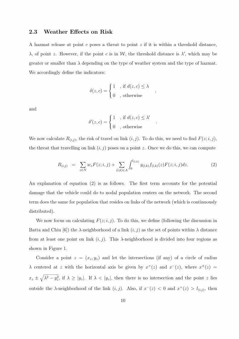
We now focus on calculating F (z; i, j). To do this, we define (following the discussion in

Batta and Chiu [6]) the λ-neighborhood of a link (i, j) as the set of points within λ distance

from at least one point on link (i, j). This λ-neighborhood is divided into four regions as

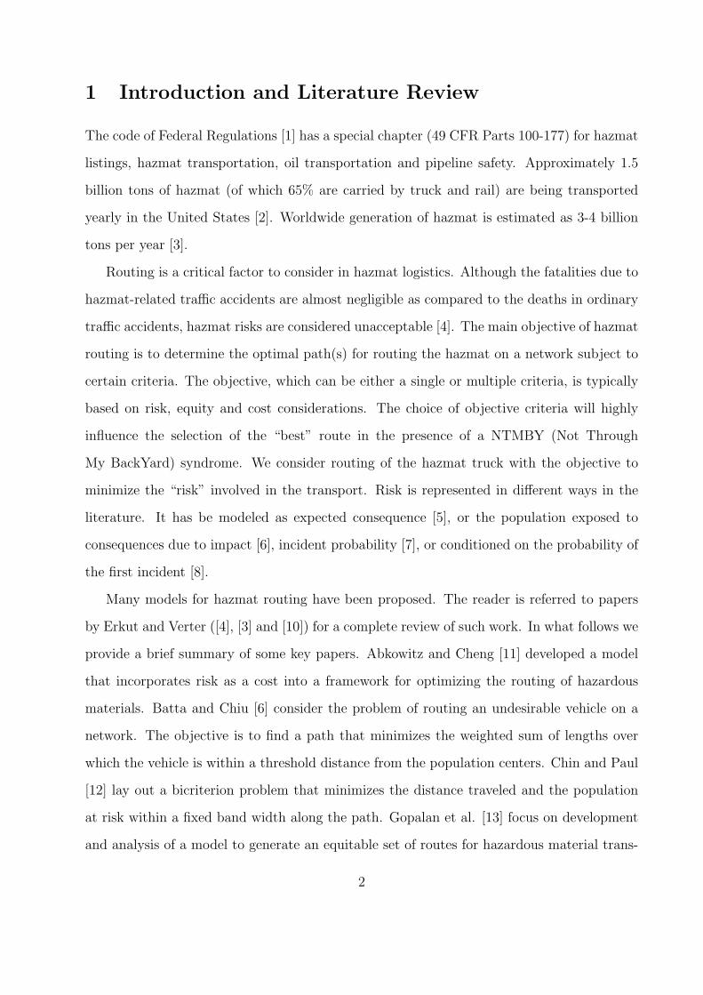
shown in Figure 1.

Consider a point z = (xz, yz) and let the intersections (if any) of a circle of radius

λ centered at z with the horizontal axis be given by x+(z) and x−(z), where x±(z) =

xz ±√

λ2 − y2z , if λ ≥ |yz|. If λ < |yz|, then there is no intersection and the point z lies

outside the λ-neighborhood of the link (i, j). Also, if x−(z) < 0 and x+(z) > l(i,j), then

10

IV

IV

II IIII

λλ

i j

Figure 1: λ-Neighborhood of Link (i, j).

the point z lies outside the λ-neighborhood of the link (i, j). The remaining situations are

identified by the regions labelled I, II, III and IV in Figure 1.

We are now armed with the notation and concepts we need to calculate F (z; i, j), the

threat that travelling on link (i, j) poses on a point z. Consider the case x(t∗1) ∈ (0, l(i,j))

and x(t∗2) ∈ (0, l(i,j)). (Other cases will be handled similarly.) Clearly, x(t∗1) ≤ x(t∗2). For

this situation,

F (z; i, j) = hiδ(z, i) +∫ x(t∗1)

0q(i,j)δ(z, (y, 0))dy +

∫ x(t∗2)

x(t∗1)q′(i,j)δ

′(z, (y, 0))dy

+∫ l(i,j)

x(t∗2)q(i,j)δ(z, (y, 0))dy + hjδ(z, j). (3)

Equation (3) can be explained as follows. The first and last terms account for the possibility

of an accident at node i and node j, respectively, which in this case occur with the vehicle

outside the weather systemW . The second and fourth terms are to account for the possibility

of an accident along the link before entering and after exiting W , respectively. The third

term is for an accident along the link while in W .

We note that equation (3) is valid for the case where the vehicle starts at i and ends at j.

When computing the total risk of a path that had multiple links, using equation (3) would

double count accident probabilities on intermediate nodes of the path. As pointed out in

11

Batta and Chiu [6], this can be handled by using hi/2 and hj/2 (instead of hi and hj) for

intermediate nodes i and j. Thus, equation (3) and its variants (that account for the other

cases) can be used together with equation (2) to find the total risk associated with a specific

path for the vehicle on the network.

3 Routing Methods

In Section 2, we analyzed the movement of a vehicle to determine the risk of travel on the

link and the time taken to traverse the link in the presence of a weather system crossing the

link. These time-varying link weights are now utilized to route the vehicle across a network.

Suppose that the vehicle must start at an origin node, O, at time t = 0, and reach the

destination node, D, by time t = T . Our objective is to find the least risk path for this

vehicle from the origin to the desitnation. Since the risk and time to traverse a link are time

dependent due to weather systems, this reduces to an one-to-one time-dependent shortest

path problem (TDSPP).

3.1 Time Dependent Shortest Path Problem (TDSPP)

We can solve the TDSPP using an “exact” algorithm – this method is exact under the

premise that time has been discretized finely enough. To do this we can use a O(|N |3M2)

label correcting algorithm that is described in Ziliaskopolus and Mahamassani [27], here M is

a large integer such that t0 to t0 +Mδ is time interval of interest, t0 is the starting time, and

δ is a small time interval during which weather conditions remain unchanged. We refer the

reader to [27] for details about the procedure. The only modification in our implementation of

this procedure is that we use the modified link lengths calculated as described in Section 2.3.

Memory and computational requirements can be reduced by finding an upper bound, Ui,

and lower bound, Li for the possible arrival times at node i. In this way there are fewer

labels for each node. This can be achieved as follows:

1. Find for each link the minimum possible travel time t∗ij = min{t∗ij(t)} t = 1, 2, . . . , T .

12

2. Use Djikstra’s labeling algorithm to find the minimum travel time (using t∗ij ) between

the origin and all other nodes (including the destination). Let the minimum arrival

time to a node j be Lj. Therefore the minimum time label for node j is t = Lj.

3. Use Djikstra’s labeling algorithm to find the minimum travel time (using t∗ij ) between

a node and the destination. Let the minimum arrival time from node j to destination

be Uj. Then T − Uj is the latest possible departure time from node j so that the

destination is not reached later than T . Therefore this is the maximum time label for

node j.

The TDSPP algorithm essentially permits parking after every δ units of time. Thus an

optimal path may have numerous instances of parking, i.e. the vehicle may be scheduled to

stop several times enroute to the destination. In practice there are likely to be limitations on

the number of times the hazmat carrying truck can park and also the minimum/maximum

amount of time that it should park. The algorithm doesn’t take this into consideration.

Hence the algorithm will give much lower risk values than are practically possible. Also, due

to memory and computation time limitations, this algorithm can be used realistically only

for small-sized networks. The computational runs showed that the algorithm could solve

a path between O-D pairs whose path length varied from 122 to 845 miles with run times

varying from 3 to 51 minutes. In these runs, time was discretized in intervals of 5 minutes.

As the time intervals are made smaller and/or the network size increases, the computational

time and memory requirements become highly intensive. For this reason, in the rest of this

section we describe several heuristic methods (based on similar algorithms available in the

literature) which can be used for solving practical problems. These methods are designed to

work in reasonable time and also limit the number of parking opportunities to just one.

3.2 k-Shortest Path Heuristic (KPATH)

A logical approach is to search through a set of paths and select the best one. In this

heuristic, a set of k-shortest paths is found for the network with time-invariant weights and

13

these paths are then evaluated using time-variant weights. The paths are evaluated for

improvement due to parking at a node, and the path with the least weight is selected. The

steps involved in the KPATH heuristic are as follows:

1. Yen’s k-shortest path algorithm [29] is used with static weights i.e. the expected risk

calculated ignoring the weather system effects. The expected risk ignoring the weather

system effects is calculated using the procedure laid out in [6]. This is used as link

weights to generate the k shortest paths.

2. After this set of shortest paths is found, the weight of each path is evaluated with the

dynamic weights.

3. The slack time for each path is calculated. The initial value of slack time is the

difference between the travel time of the path and T , the maximum time allowed by

which the shipment has to reach destination node D.

4. Each path is evaluated for improvement by assigning all the slack time to a node on

the path.

5. If the destination is not reached by time T due to addition of this slack, i.e. parking on

the node, then the slack is reduced by one unit and the procedure is repeated iteratively

till the time constraint is met.

6. Steps 4 and 5 are repeated for each node on the vehicle’s path and the best solution is

reported.

Thus, each path is optimized by considering parking at every node on the path such

that the T time limit is met. The path with the least consequence is selected. For the

problems we considered, the travel time is less than ten hours, so in a practical sense the

driver would stop at most once, rather than making several small stops as suggested by the

TDSPP algorithm. The fact that we choose to do an “all or nothing” parking assignment is

justified by the result of Theorem 1.

14

A potential drawback of this heuristic is the fact that most of the k shortest paths are

small variations of each other. Therefore, it will likely be difficult to find spatially dissimilar

and feasible paths to avoid the weather systems unless k is very large – which increases the

computational time and memory requirements substantially.

3.3 Dissimilar Path Heuristic (DISSIM)

Another heuristic is based on the dissimilar path method [30]. In this heuristic, a set of paths

is first found by using either the KPATH or IPM [31]. The dissimilar path method [30] is

then applied to obtain a subset of paths of maximum disparity. A stricter time limit of T ∗

is set, which accounts for the travel time increase due to weather systems. Paths obtained

from the dissimilar path method with travel time greater than T ∗ are discarded. Then the

remaining paths are evaluated with the dynamic weights, and for benefits due to parking

using the same procedure as in the KPATH Heuristic. The advantage of this method is

that it has the potential of identifying spatially dissimilar paths that may avoid the weather

systems.

3.4 Iterative Weather System Heuristic (IWS)

This heuristic is based on the “Iterative Penalty Method” [31], where the procedure first finds

the shortest path, and then penalizes the arcs (or nodes) on this path using a preset penalty

factor. The two-step procedure continues until the desired number of alternate paths are

found. In the IWS the penalties are based on the dynamic weights induced by the weather

system(s). Steps of the heuristic are as follows:

1. Find the optimal path with static weights and save it as an incumbent solution.

2. Calculate the link weights by incorporating the weather system effects.

(a) If there is no change in the link weights, then the current path is optimal.

(b) Else update the weights for the affected links.

3. Repeat until

(a) there is no change in the link weights, or

15

(b) the current path is identical to the incumbent path.

The advantages of this heuristic over the IPM are (i) the penalty mechanism is simple

and fixed, and (ii) only the links that are affected by the weather system are penalized.

However, there are drawbacks: these penalties are permanent. When a link is penalized,

it is based on the time when the vehicle enters the link. However, the same weight is used

in the subsequent iterations even though the entry time of the link may be different under

different paths that utilize that link.

The stopping criteria could be changed so that even if the current path is identical to

the incumbent, the links affected could be penalized again, and a new path could be found

either until no weight change occurs or a threshold number of iterations are performed with

no change in the incumbent path. The path obtained using the IWS is then evaluated for

improvement using the available slack time as described in Section 3.2.

3.5 Myopic Shortest Path Heuristic (MYOPIC)

This heuristic uses time-dependent link weights in a greedy manner to find a solution to

the time-dependent shortest path problem. The only difference between this method and

traditional shortest path method is that the link weights are calculated dynamically due to

the time-dependent weights. First the minimum temporary label is selected and then it is

made permanent after the adjacent nodes with temporary labels are checked for updates.

The final path got from the heuristic is evaluated for improvement due to parking using the

method described in Section 3.2.

The drawback of this heuristic is that it keeps just one label for each node regardless of

the entrance time to the node. For example, consider two partial paths P1 and P2 from the

origin to node i with total weights of w1 and w2 and with arrival times t1 and t2, respectively.

Assume that w1 < w2 and t1 6= t2. According to the heuristic, P1 will dominate P2 even

though t1 and t2 are not equal. It is very well possible that the path P2 could end with

a shorter path since the weight of the further links are time-dependent. The only way to

overcome this drawback is to keep multiple labels for each node, which turns out to be the

16

exact algorithm for this problem.

4 Computational Framework

In this section we describe the computational framework that we developed to test the

TDSPP algorithm and the heuristics developed in Section 3. The analysis was conducted

under a variety of conditions. All methods were coded using C++ and Java and implemented

on a Pentium III, 800 Mhz personal computer with 392 MB of memory. The TDSPP

algorithm was implemented by dynamically increasing the number of labels for nodes instead

of allocating the memory at the beginning. Dynamic memory usage was also employed with

the heuristics whenever applicable.

4.1 Network Development

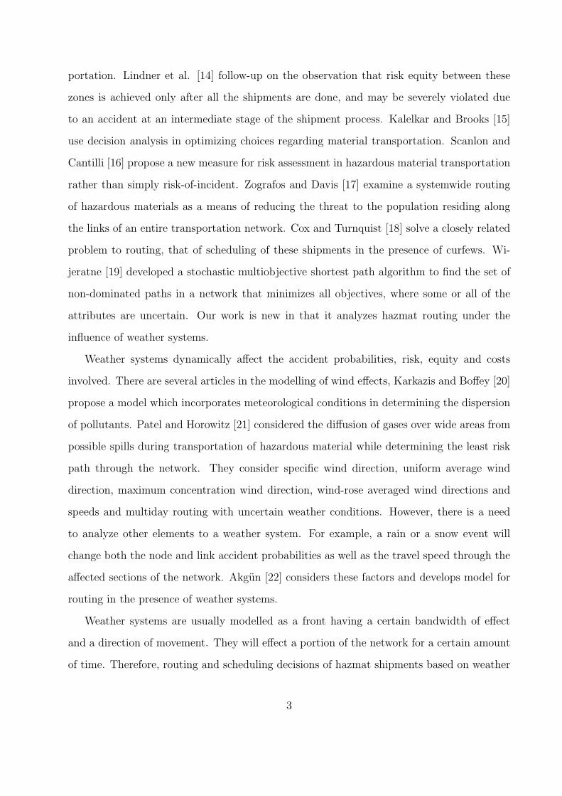
The network of the State of Texas is used to implement the exact algorithm and heuristics.

We used the road data from the National Transportation Atlas Databases (1997), NTAD97,

from the Bureau of Transportation Statistics. We included interstate, US and State highways

in the network. County highways, local and rural roads have been excluded. There are 5,521

nodes and 6,756 links in our network, which is depicted in Figure 2.

Average speeds for the interstate, US and State highways were considered to be 65, 55 and

50 miles per hour, respectively. Certain link attributes such as accident rates and population

at risk are not included in NTAD97. Calculation of these attributes as well as incorporating

weather systems are discussed below.

4.2 Calculation of Link Attributes

4.2.1 Accident Rates

For illustrative purposes in this research, we used the accident rates from a Highway Safety

Information System report [28] that used truck accident data from Utah for 1985-1987 to

determine truck accident rates as a function of road type. We assumed that the adverse

17

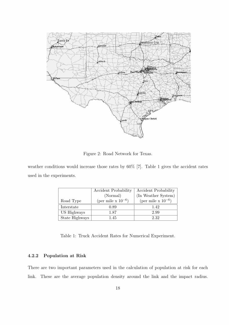
Figure 2: Road Network for Texas.

weather conditions would increase those rates by 60% [7]. Table 1 gives the accident rates

used in the experiments.

Accident Probability Accident Probability(Normal) (In Weather System)

Road Type (per mile x 10−6) (per mile x 10−6)Interstate 0.89 1.42US Highways 1.87 2.99State Highways 1.45 2.32

Table 1: Truck Accident Rates for Numerical Experiment.

4.2.2 Population at Risk

There are two important parameters used in the calculation of population at risk for each

link. These are the average population density around the link and the impact radius.

18

Population at risk is calculated by multiplying the population density within the area of a

circle of the given radius. The impact radius is entered by the user and was taken as two

miles for the initial analysis. Note that the radius may depend on the type of hazardous

materials and weather conditions.

Link population densities were calculated by using census data from the 1990 TIGER

database. The entire US is divided into polygons by the census bureau. Population within

each polygon and the area of each polygon are known. Population density is assumed to

be uniform within a polygon. Each link is defined by shape points so that the location of

the link could be portrayed graphically. For example, a link with 14.68 miles length in our

network has 73 shape points, each of which is defined by longitude and latitude. In order to

determine the average population density of a link, we overlayed the shape points of the link

with the census polygons by using Geographic Information System (GIS) software, recording

the population density for each shape point. Then, we took the average of these values to

find the approximate population density of the link.

Using approximate population densities, we were able to approximate the expected pop-

ulation at risk for a given radius. There are different ways of calculating the population at

risk such as calculating the total population at risk for a given bandwidth around the link.

Since our main objective is to focus on the effects of weather systems, we chose one of these

methods for illustrative purposes.

4.2.3 Weather Systems

We assume the weather systems to be circular with a constant radius, speed and direction.

We also assume that the initial location of a weather system is known. The number of

weather systems varied between three and five. As defaults, we set the impact radius of a

weather system as two miles and assumed the vehicle travel speed is 25% less in a weather

system. The method explained in Section 2 was used to calculate the link travel time and

accident probabilities dynamically.

If there are multiple weather systems affecting the same link, entrance and departure

19

times are calculated for each weather system. Then, the union of these intervals is found. For

example, consider a link that is affected by three weather systems, which have entrance and

departure time intervals of [1, 3], [2, 4] and [5, 7]. The union of these intervals is {[1, 4], [5, 7]}.The underlying assumption in this calculation is that the slower travel due to the first weather

system does not affect the critical times for the second weather system and so on. Given the

fact that the link lengths are very small in the NTAD97 database, it would be unlikely for

a short link to be affected by more than one weather system at different time intervals, so

this drawback is not significant.

5 Computational Experiments

We focused on three goals for the numerical experiments. Firstly, we test the behavior of

the TDSPP algorithm for different values of δ since its performance depends on how finely

time is discretized. We then empirically determine the size of problems that can be solved

to optimality in less than one hour. Our main goal was to determine how well the heuristics

perform for these problems. Finally, we implemented the heuristics on larger-scale problems

to compare them in terms of solution quality and solution time.

We limited the number of paths for the KPATH heuristic to ten paths. Also we imple-

mented the DISSIM heuristic by using the ten paths generated by the KPATH heuristic,

selecting five dissimilar ones. Expected consequence is the sum-product of the accident

probabilities and the population for the links on the selected path.

In the tables that follow, algorithm runtime is given in seconds, travel distance is given

in miles, and travel time in minutes. The ‘number of nodes’ column represents the number

of nodes on the solution path.

5.1 Performance Analysis of TDSPP Algorithm

The performance of the exact algorithm is studied for ten origin-destination (O-D) pairs, for

different values of δ. The values of δ considered are 1, 5, 10, 15, 20, and 25. For these ten

problems the computational runtime decreases as the δ is increased. The number of weather

20

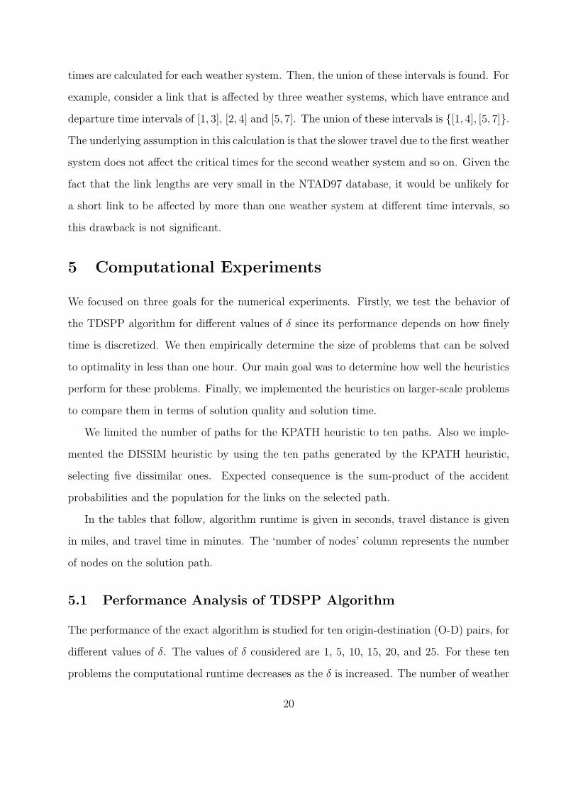
systems was varied between one to five. Since the results show similar characteristics across

the O-D pairs, we only present the results for one such O-D pair in Table 2.

Origin - Destination Pair 1

Time Travel Travel No. of Expected Algorithm

Interval Distance Time Nodes Effect Runtime

δ x 10−4

1 115.5 163 14 1.29 1819

5 115.5 165 14 1.29 1714

10 15.5 160 3 2.41 467

15 15.5 150 3 2.41 202

20 15.5 140 3 2.41 119

25 15.5 125 3 2.41 65

Table 2: Performance of TDSPP Algorithm for O-D Pair 1.

Here, the large difference in travel distances is because the first two solution paths (for

δ = 1, 5), minimize the risk of the path by taking a longer route with little parking. The

path taken avoids the weather system by selecting links that are not affected by the weather

system. The remaining paths (for δ = 10, 15, 20 and 25) follow a much shorter route in terms

of travel distance (this is also reflected in the number of nodes visited by the paths) and

exhibit extensive parking times. The results prove the importance of selecting an appropriate

value for δ. It can be observed that as the value of δ is decreased the computational runtime

increases dramatically. It should be also stated that as δ decreases the memory requirements

increases as we are storing labels for each time interval. Furthermore, it must be noted that

as the value of δ is increased the solution obtained from the algorithm varies. It can be seen

in Table 2 that the path obtained from the algorithm changes for a value of δ > 5 minutes.

Thus the value of δ affects solution quality. The question we are faced with is: How finely

should the time be discretized to assure the optimality of the algorithm? The answer to this

depends on the network, the time limit for reaching the destination, the weather systems,

acceptable runtime and memory constraints.

21

5.2 Comparison of Heuristic Methods with TDSPP

We determined ten origin-destination (O-D) pairs, for which the length of the minimum

consequence path varied between 122 and 845 miles. For these ten problems, the solution

time of the TDSPP algorithm varied between 3 seconds and 51 minutes. The solution time

for the TDSPP algorithm strongly depends on the location of the origin and the destination

if the road network is dense, then the solution time tends to be higher.

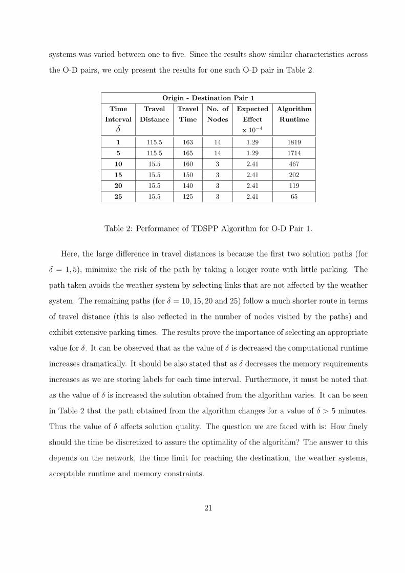
Since the results for the different O-D pairs are similar, we present the results for one

of the time consuming O-D pair in Table 3. We normalized the expected consequence value

along the optimal route between this O-D pair to a baseline of 1.0 in order to make the

comparison easier.

Algorithmic Travel Travel No. of Normalized Algorithm

Method Distance Time Nodes Expected Runtime

Effect

KPATH 701.1 765 42 1.16 425

DISSIM 701.1 765 42 1.16 589

IWS 571.4 803 48 1.14 405

MYOPIC 652.5 1014 56 1.13 388

TDSPP 652.5 934 56 1.00 1853

Table 3: Comparison of Heuristic Methods with TDSPP.

For this O-D Pair, none of the heuristics was able to find the minimum consequence path

of TDSPP, yet all, found a path within 16% of optimality. Also, all the heuristics required

much less computation time than the optimal algorithm. The main reason due to which

there is such a significant difference in the solution quality between the TDSPP algorithm

and the heuristics is parking. The TDSPP method allows for a very large number of parking

opportunities, whereas the heuristics only allow for at most one such opportunity. Since,

in practice, there are significant limitations on the number of times parking can be done

to avoid weather systems, the heuristic results are likely to be much more reasonable than

would be otherwise indicated by Table 3.

22

Comparing the heuristics we find that KPATH and DISSIM perform the worst. Of the

other heuristics, MYOPIC found the best path. Its best path (near 13% of optimality) was

not found by the other heuristics. The second-best path (at 14%) was found by IWS and

the third-best path (at 16%) was found by KPATH and DISSIM. The path for the KPATH

and DISSIM heuristics are identical, which is not surprising given the fact that the DISSIM

heuristic selected from the KPATH set of paths.

The effect of the weather systems on the consequence is apparent if we examine the paths

that are generated. The paths try to avoid links that are affected by the weather systems.

The main reason for this is the increase in accident probabilities and hence consequence

due to the weather systems. Details of these paths are not shown for the sake of brevity.

Interested readers can view these details in the recent thesis by Parekh [32].

5.3 Comparison of Heuristics for Large Problems

As the size of the problem increases, the TDSPP algorithm becomes very slow and compu-

tationally demanding. For larger-scale problems, we suggest that the heuristic methods be

used. We therefore, test the heuristics for larger problems.

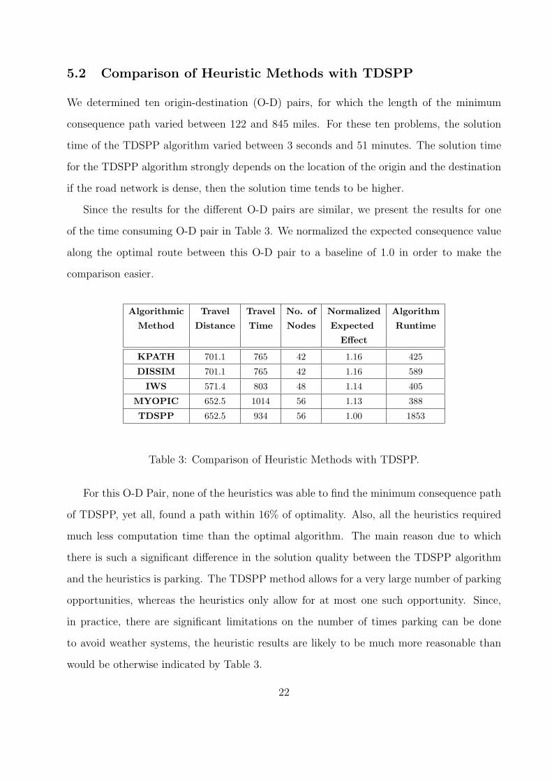
We again selected ten O-D pairs, for which the length is about three times larger than

the routes considered in Section 5.2. The computational results for three representative O-D

Pairs 1, 3 and 6 are presented in Tables 4, 5 and 6, respectively.

Origin - Destination Pair 1

Algorithmic Travel Travel No. of Expected Algorithm

Method Distance Time Nodes Effect Runtime

x 10−3

KPATH 2369.8 2567 127 9.1538 1236

DISSIM 2369.8 2567 127 9.1538 536

IWS 2193.2 2393 108 5.7831 344

MYOPIC 2193.2 2393 108 5.3015 294

Table 4: Comparison of Heuristic Methods for O-D Pair 1.

23

Origin - Destination Pair 3

Algorithmic Travel Travel No. of Expected Algorithm

Method Distance Time Nodes Effect Runtime

x 10−3

KPATH 97.5 107 25 2.0276 116

DISSIM 37.8 42 20 3.5384 38

IWS 87.6 98 23 1.1573 276

MYOPIC 81.1 119 19 1.0211 63

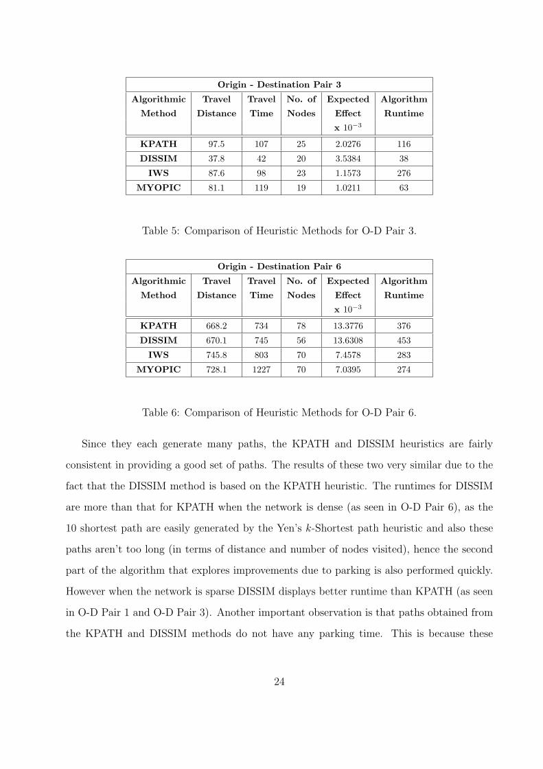
Table 5: Comparison of Heuristic Methods for O-D Pair 3.

Origin - Destination Pair 6

Algorithmic Travel Travel No. of Expected Algorithm

Method Distance Time Nodes Effect Runtime

x 10−3

KPATH 668.2 734 78 13.3776 376

DISSIM 670.1 745 56 13.6308 453

IWS 745.8 803 70 7.4578 283

MYOPIC 728.1 1227 70 7.0395 274

Table 6: Comparison of Heuristic Methods for O-D Pair 6.

Since they each generate many paths, the KPATH and DISSIM heuristics are fairly

consistent in providing a good set of paths. The results of these two very similar due to the

fact that the DISSIM method is based on the KPATH heuristic. The runtimes for DISSIM

are more than that for KPATH when the network is dense (as seen in O-D Pair 6), as the

10 shortest path are easily generated by the Yen’s k-Shortest path heuristic and also these

paths aren’t too long (in terms of distance and number of nodes visited), hence the second

part of the algorithm that explores improvements due to parking is also performed quickly.

However when the network is sparse DISSIM displays better runtime than KPATH (as seen

in O-D Pair 1 and O-D Pair 3). Another important observation is that paths obtained from

the KPATH and DISSIM methods do not have any parking time. This is because these

24

heuristics use paths that avoid the weather system.

Among the heuristics, the IWS and MYOPIC heuristics typically find the best solution.

Also, the IWS and MYOPIC heuristics usually have shorter runtimes than the other heuris-

tics. It should be noted though that when we have most of the links of the path affected by

weather systems, as in Table 4 for O-D Pair 3, the runtimes for IWS are significantly higher.

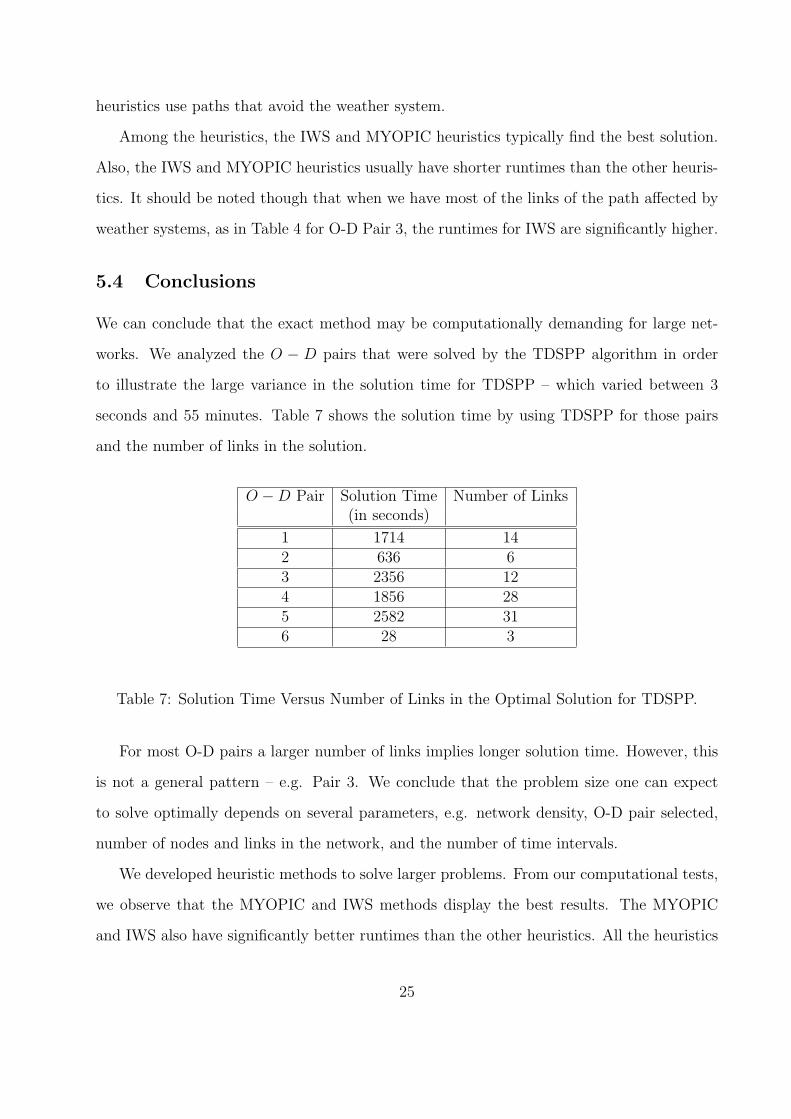
5.4 Conclusions

We can conclude that the exact method may be computationally demanding for large net-

works. We analyzed the O − D pairs that were solved by the TDSPP algorithm in order

to illustrate the large variance in the solution time for TDSPP – which varied between 3

seconds and 55 minutes. Table 7 shows the solution time by using TDSPP for those pairs

and the number of links in the solution.

O −D Pair Solution Time Number of Links(in seconds)

1 1714 142 636 63 2356 124 1856 285 2582 316 28 3

Table 7: Solution Time Versus Number of Links in the Optimal Solution for TDSPP.

For most O-D pairs a larger number of links implies longer solution time. However, this

is not a general pattern – e.g. Pair 3. We conclude that the problem size one can expect

to solve optimally depends on several parameters, e.g. network density, O-D pair selected,

number of nodes and links in the network, and the number of time intervals.

We developed heuristic methods to solve larger problems. From our computational tests,

we observe that the MYOPIC and IWS methods display the best results. The MYOPIC

and IWS also have significantly better runtimes than the other heuristics. All the heuristics

25

evaluate for improvement by allowing parking at a single node on the path. The heuristics

either avoid the weather system effects by parking at a strategic location and time (MY-

OPIC and IWS) or by using alternate links that are not influenced by the weather system

(KPATH and DISSIM). The latter strategy, however, results in paths that have higher travel

distances.

6 Future Research

We end this paper by stating two directions for future work in this area.

A possible extension of this work is for an environment in which there is uncertainty

associated with the size and movement of a weather system. The level of complexity in such

a situation can be decreased by using Geographical Information Systems (GIS) to capture,

store, manipulate, analyze and display the spatially referenced and associated tabular data

needed for these algorithms [33].

Another fruitful direction for future research is to incorporate the risk due to parking

in the model. We have assumed that there is zero risk when the vehicle carrying hazmat

is parked. This is not realistic since accidents are possible (though admittedly less likely)

when a vehicle is parked.

References

[1] Code of Federal Regulations, 49 CFR Parts 1995;100-177.

[2] Abkowitz M, Cheng PD, Lepofsky M. Use of Geographic Information Systems in Manag-

ing Hazardous Materials Shipments. Transportation Research Record 1990;1261:35–43.

[3] Erkut E, Verter V. Hazardous Materials Logistics: A review. Drezner, Z. (ed.). Facility

Location: A Survey of Applications and Methods. NY: Springer-Verlag, 1994.

26

[4] Erkut E, Verter V. Hazardous Materials Logistics: An Annotated Bibliography. Op-

erations Research and Environmental Management. Haurie A, Carraro C. (eds.):

KLUWER International Series on Economics, Energy and Environment, 1994.

[5] Erkut E, Verter V. A Framework for Hazardous Materials Transport Risk Assessment.

Risk Analysis 1995;15:589–601.

[6] Batta R, Chiu S. Optimal Obnoxious Paths on a Network: Transportation of Hazardous

Materials. Operations Research 1988;36(1):84–92.

[7] Saccomanno FF, Chan AY-W. Economic Evaluation of Routing Strategies for Hazardous

Road Shipments. Transportation Research Record 1985;1020:12–18.

[8] Abkowitz M, Cheng PD. Selecting Criteria for Designing Hazardous Materials Highway

Routes. Transportation Research 1992;1333:30–35.

[9] Sivakumar RA, Batta R, Karwan MH. A Multiple Route Conditional Risk Model

for Transporting Hazardous Materials. Information Systems and Operational Research

1995;33:20–33.

[10] Erkut E, Verter V. Modeling of Transport Risk for Hazardous Materials. Operations

Research 1999;77(7):777–787.

[11] Abkowitz M, Cheng PD. Developing a Risk-Cost Framework for Routing Truck Move-

ments of Hazardous Materials. Accident Analysis & Prevention 1988;20:39–51.

[12] Chin S, Paul DC. Bicriterion Routing Scheme for Nuclear Spent Fuel Transportation.

Transportation Research Record 1989;1245:60–64.

[13] Gopalan R, Kolluri S, Batta R, Karwan M. Modeling Equity of Risk in the Transporta-

tion of Hazardous Materials. Operations Research 1990;38(6):961–973.

[14] Lindner-Dutton L, Batta R, Karwan M H. Equitable Sequencing of a Given Set of

Hazardous Materials Shipments. Transportation Science 1991;25(2):124–137.

27

[15] Kalelkar AS, Brooks RE, Use of Multidimensional Utility Functions in Hazardous Ship-

ment Decisions. Accident Analysis & Prevention 1978;10:251–265.

[16] Scanlon RD, Cantilli EJ. Assessing the Risk and Safety in the Transportation of Haz-

ardous Materials. Transportation Research Record 1985;1020:6–11.

[17] Zografos KG, Davis CF. Multi-objective Programming Approach for Routing Hazardous

Materials. Journal of Transportation Engineering 1989;115(6):661–673.

[18] Cox RG, Turnquist MA. Scheduling Truck Shipments of Hazardous materials in the

Presence of Curfews. Transportation Research Record 1986;1063:21–26.

[19] Wijeratne AB. Routing and Scheduling Decisions in the Management of Hazardous

Material Shipments; Ph.D. Dissertation, Department of Civil and Environmental Engi-

neering, Cornell University, Ithaca, NY, 1990.

[20] Karkazis J, Boffey TB. Optimal Location of Routes for Vehicles Transporting Hazardous

Materials. European Journal of Operational Research 1995;86:201–215.

[21] Patel MH, Horowitz AJ. Optimal Routing of Hazardous Materials Considering Risk of

Spill. Transportation Research-A 1994;28A(2):119–132.

[22] Akgun, V. Routing of Hazardous Materials in the Presence of Weather Systems, Unpub-

lished Ph.D. Dissertation, Department of Industrial Engineering, University at Buffalo,

SUNY, Buffalo, NY, 14260, 2001.

[23] Cooke KL, Halsey, E. The Shortest Route Through a Network with Time-Dependent

Inter-Nodal Transit Times. Journal of Mathematical Analysis and Applications

1966;14:493–498.

[24] Dreyfus SE. An Appraisal of Some Shortest-Path Algoritms. Operations Research

1969;17:395–412.

[25] Djikstra EW. A Note on Two Problems in Connexion with Graphs. Numerical Mathe-

matics 1959;1:269–271.

28

[26] Orda A, Rom R. Shortest-Path and Minimum-Delay Algorithms in Networks with Time-

Dependant Edge-Lengths. Journal of the ACM 1990;37:607–625.

[27] Ziliaskopoulos AK, Mahmassani HS. Time-Dependent, Shortest-Path Algorithm for

Real-Time Intelligent Vehicle Highway System Applications. Transportation Research

Record 1993;1408:94–100.

[28] US Department of Transportation, Truck Accident Models. HSIS Summary Report.

FHWA-RD-94-022, 1994.

[29] Yen JY. Finding the K-Shortest Loopless Paths in a Network. Management Science

1971;17(11):712-716.

[30] Akgun V, Erkut E, Batta R. On Finding Dissimilar Paths. European Journal of Oper-

ational Research 2000;121:232–246.

[31] Johnson PE, Joy DS, Clarke DB, Jacobi JM. HIGHWAY 3.01, An Enhanced Highway

Routing Model: Program, Description, Methodology, and Revised User’s Manual, Oak

Ridge National Laboratory, ORNL/TM-12124, Oak Ridge, TN, 1992.

[32] Parekh A. Time Dependent Shortest Path Algorithms For Routing of Hazardous Ma-

terials in the Presence of Weather Systems. Unpublished M.S. Thesis, Department of

Industrial Engineering, University at Buffalo, SUNY, Buffalo, NY, 14260, 2003.

[33] Fischer MM, Nijkamp P. Geographic Information Systems, Spatial Modeling, and Policy

Evaluation: Springer-Verlag, 1993.

29