ROUTING IN MIXED WIRED AND WIRELESS NETWORKS

APPROVED BY SUPERVISING COMMITTEE:

Dr. Rajendra V. Boppana, Supervising Professor

Dr. Ki Hwan Yum

Dr. Ali S. Tosun

Accepted:

Dean of Graduate School

ROUTING IN MIXED WIRED AND WIRELESS NETWORKS

by

ZHI ZHENG, B.E

THESISPresented to the Graduate Faculty of

The University of Texas at San Antonioin Partial Fulfillmentof the Requirementsfor the Degree of

MASTER OF SCIENCE IN COMPUTER SCIENCE

THE UNIVERSITY OF TEXAS AT SAN ANTONIOCollege of Sciences

Department of Computer ScienceDecember 2004

Acknowledgements

I would like to express sincere gratitude for the time, encouragement and guidance by Dr. Rajendra V.

Boppana, my supervisor. His intelligence, insights and hardworking has been very valuable for this thesis

and for myself.

Thanks for Dr. Ali S. Tosun and Dr. Ki Hwan Yum for serving on my committee and thanks for all the

support from my colleagues and the computer science department in UTSA. I express my gratitude to the

Computer Science Division and its staff for extending excellent co-operation at all the times.

May 2004

iii

ROUTING IN MIXED WIRED AND WIRELESS NETWORKS

Zhi Zheng, B.E.The University of Texas at San Antonio, 2004

Supervising Professor: Dr. Rajendra V. Boppana

The last decade has witnessed an explosion in wireless networking technologies such as cellular and Wi-

Fi. While these new technologies provide flexible and mobile networkings, they are either expensive or

unreliable. So, we believe the future local and metropolitan area network will consist of fixed or stationary

devices acting as infrastructure nodes and wireless devices connecting mobile users.

Recent advances in technology make such networks feasible and desirable. Such networks can replace

DSL/Cable modem or cellular service. Problems to be solved to make such networks viable include the de-

sign and update of network hardware devices, the software such as routing protocol, the security mechanism

and applications.

Our research focuses on the design of a suitable routing protocol and performance evaluation of networks

with mixed broadcast type wireless and point-to-point (p2p) links. In this thesis, we present ADV static

(ADVS) routing algorithm which can use both p2p and broadcast (wireless) links to route messages. ADVS

is based on the Adaptive Distance Vector (ADV) routing protocol, designed for mobile ad hoc networks. We

use simple changes to route selection logic to promote the use of wired links when feasible. We implemented

ADVS in the Glomosim simulator, which is widely used in wireless ad hoc network studies. We also

modified Glomosim to simulate networks with (a) both wireless and p2p links and (b) mobile and fixed

nodes simultaneously.

iv

To evaluate the performance benefits of mixed networks over ad hoc wireless networks, we simulated

both types of networks with ADVS as the routing protocol. We considered UDP and TCP traffic patterns. In

all cases, the mixed networks provide better throughput and packet delays. The throughput gains with a few

point-to-point links added to an otherwise ad hoc network can double throughput and halve packet delays

even when point-to-point and wireless links have the same bandwidth.

v

TABLE OF CONTENTS

Acknowledgements . . . . . . . . . . . . . . . . . . . . . . . . . . . . . . . . . . . . . . . . . . . . . . . . . . . . . . . . . . . . . . . . . . . . . . . iii

Abstract . . . . . . . . . . . . . . . . . . . . . . . . . . . . . . . . . . . . . . . . . . . . . . . . . . . . . . . . . . . . . . . . . . . . . . . . . . . . . . . . . . iv

List of Figures . . . . . . . . . . . . . . . . . . . . . . . . . . . . . . . . . . . . . . . . . . . . . . . . . . . . . . . . . . . . . . . . . . . . . . . . . . . . viii

1 Introduction 11.1 Next Generation Wireless Networks . . . . . . . . . . . . . . . . . . . . . . . . . . . . . . 21.2 Designing and Using Mixed Networks . . . . . . . . . . . . . . . . . . . . . . . . . . . . . 51.3 Contributions of This Thesis . . . . . . . . . . . . . . . . . . . . . . . . . . . . . . . . . . 61.4 Organization . . . . . . . . . . . . . . . . . . . . . . . . . . . . . . . . . . . . . . . . . . . 7

2 Background 82.1 Overview of IEEE 802.11 MAC layer . . . . . . . . . . . . . . . . . . . . . . . . . . . . . 10

2.1.1 Carrier Sense Multiple Access (CSMA) Protocol . . . . . . . . . . . . . . . . . . . 112.2 Routing Algorithms for Ad Hoc Networks . . . . . . . . . . . . . . . . . . . . . . . . . . . 14

3 Glomosim Simulator 183.1 Passing information across nodes . . . . . . . . . . . . . . . . . . . . . . . . . . . . . . . . 193.2 Simulating fixed and mobile nodes together . . . . . . . . . . . . . . . . . . . . . . . . . . 24

4 A Routing Algorithm for Mixed Wired and Wireless Networks 264.1 ADV Static (ADVS) Routing Algorithm . . . . . . . . . . . . . . . . . . . . . . . . . . . . 264.2 Implementation of ADV Static (ADVS) algorithm . . . . . . . . . . . . . . . . . . . . . . . 30

4.2.1 Modifications to ADV . . . . . . . . . . . . . . . . . . . . . . . . . . . . . . . . . 304.2.2 Route maintenance . . . . . . . . . . . . . . . . . . . . . . . . . . . . . . . . . . . 31

5 Performance Analysis 345.1 Simulation Setup . . . . . . . . . . . . . . . . . . . . . . . . . . . . . . . . . . . . . . . . 34

5.1.1 Node Mobility . . . . . . . . . . . . . . . . . . . . . . . . . . . . . . . . . . . . . 345.1.2 Types of Links . . . . . . . . . . . . . . . . . . . . . . . . . . . . . . . . . . . . . 355.1.3 Types of Networks . . . . . . . . . . . . . . . . . . . . . . . . . . . . . . . . . . . 355.1.4 Traffic Models . . . . . . . . . . . . . . . . . . . . . . . . . . . . . . . . . . . . . 365.1.5 Routing protocols . . . . . . . . . . . . . . . . . . . . . . . . . . . . . . . . . . . . 385.1.6 Static Routes . . . . . . . . . . . . . . . . . . . . . . . . . . . . . . . . . . . . . . 385.1.7 Metrics and Parameters . . . . . . . . . . . . . . . . . . . . . . . . . . . . . . . . . 38

5.2 Small Ad Hoc Networks . . . . . . . . . . . . . . . . . . . . . . . . . . . . . . . . . . . . 39

vi

5.2.1 UDP traffic . . . . . . . . . . . . . . . . . . . . . . . . . . . . . . . . . . . . . . . 395.2.2 TCP traffic . . . . . . . . . . . . . . . . . . . . . . . . . . . . . . . . . . . . . . . 43

5.3 Large Ad Hoc Networks . . . . . . . . . . . . . . . . . . . . . . . . . . . . . . . . . . . . 455.3.1 TCP Traffic . . . . . . . . . . . . . . . . . . . . . . . . . . . . . . . . . . . . . . . 48

6 Conclusions 50

Bibliography . . . . . . . . . . . . . . . . . . . . . . . . . . . . . . . . . . . . . . . . . . . . . . . . . . . . . . . . . . . . . . . . . . . . . . . . . . . . . 52

Vita 54

vii

List of Figures

1.1 Example of an ad hoc wireless network. . . . . . . . . . . . . . . . . . . . . . . . . . . . . 21.2 One-hop wireless networks. . . . . . . . . . . . . . . . . . . . . . . . . . . . . . . . . . . . 31.3 Mixed wired and wireless networks. . . . . . . . . . . . . . . . . . . . . . . . . . . . . . . 5

2.1 Protocol layer structure. . . . . . . . . . . . . . . . . . . . . . . . . . . . . . . . . . . . . . 92.2 DCF and PCF. (Taken from [7]) . . . . . . . . . . . . . . . . . . . . . . . . . . . . . . . . 102.3 Wireless islands or independent basic service sets (IBSS). . . . . . . . . . . . . . . . . . . . 112.4 Connected wireless islands (extended service sets, ESS). . . . . . . . . . . . . . . . . . . . 112.5 CSMA/CA. . . . . . . . . . . . . . . . . . . . . . . . . . . . . . . . . . . . . . . . . . . . 122.6 Hidden Terminal. . . . . . . . . . . . . . . . . . . . . . . . . . . . . . . . . . . . . . . . . 122.7 Transmitting a data frame in 802.11 . . . . . . . . . . . . . . . . . . . . . . . . . . . . . . 132.8 Backoff procedure in IEEE 802.11. (Taken from [7].) . . . . . . . . . . . . . . . . . . . . . 14

3.1 The event driven model and different protocol layers in Glomosim. . . . . . . . . . . . . . . 203.2 The protocol layer structure for wired and wireless transmission. . . . . . . . . . . . . . . . 213.3 The structure of network layer and MAC layer for wired transmission. . . . . . . . . . . . . 223.4 The structure of MAC layer for wireless transmission. . . . . . . . . . . . . . . . . . . . . . 233.5 The structure of radio layer. . . . . . . . . . . . . . . . . . . . . . . . . . . . . . . . . . . . 24

4.1 Dissemination of routing information in ad hoc wireless networks. . . . . . . . . . . . . . . 274.2 Dissemination of routing information in mixed wired and wireless networks. . . . . . . . . . 274.3 Data transmission in ad hoc wireless networks. . . . . . . . . . . . . . . . . . . . . . . . . 294.4 Data transmission in mixed wired and wireless networks. . . . . . . . . . . . . . . . . . . . 29

5.1 Fifty-node wireless network in a field of 1500m x 1500m. . . . . . . . . . . . . . . . . . . . 365.2 Fifty nine-node wireless network with 50 mobile and 9 fixed nodes. . . . . . . . . . . . . . 375.3 Mixed network with 50 mobile nodes and 9 fixed nodes. . . . . . . . . . . . . . . . . . . . 375.4 Throughputs achieved for CBR traffic on 50/59-node ad hoc networks. . . . . . . . . . . . . 405.5 Delivery rate on 50/59-node ad hoc networks. . . . . . . . . . . . . . . . . . . . . . . . . . 405.6 The number of wireless hops taken by each data packet on 50/59-node ad hoc networks. . . 405.7 Overheads on wireless links achieved for CBR traffic on 50/59-node ad hoc networks. . . . . 405.8 Average Network Allocation Vector(NAV) on 50/59-node ad hoc networks. . . . . . . . . . 425.9 Average broken routes on 50/59-node ad hoc networks. . . . . . . . . . . . . . . . . . . . . 425.10 Average delays achieved for CBR traffic on 50/59-node ad hoc networks. . . . . . . . . . . 425.11 Average delays (offerloads from 0 to 80 kbps) achieved for CBR traffic on 50/59-node ad

hoc networks. . . . . . . . . . . . . . . . . . . . . . . . . . . . . . . . . . . . . . . . . . . 425.12 Throughputs achieved for HTTP traffic on 50/59-node ad hoc networks. Each server has

one client. . . . . . . . . . . . . . . . . . . . . . . . . . . . . . . . . . . . . . . . . . . . . 43

viii

5.13 Throughputs achieved for HTTP traffic on 50/59-node ad hoc networks. . . . . . . . . . . . 435.14 Overheads on wireless links achieved for HTTP traffic on 50/59-node ad hoc networks. . . . 445.15 Overheads on wireless links achieved for HTTP traffic on 50/59-node ad hoc networks. . . . 445.16 Throughputs achieved for FTP traffic on 50/59-node ad hoc networks. . . . . . . . . . . . . 445.17 Overheads achieved for FTP traffic on 50/59-node ad hoc networks. . . . . . . . . . . . . . 445.18 Throughputs achieved for CBR traffic on 1000-node ad hoc networks. . . . . . . . . . . . . 455.19 Delivery rates for CBR traffic on 1000-node ad hoc networks. . . . . . . . . . . . . . . . . . 455.20 The number of wireless hops taken by a data packet in 1000-node ad hoc networks. . . . . . 475.21 Overheads on wireless links achieved for CBR traffic on 1000-node ad hoc networks. . . . . 475.22 Average Network Allocation Vector(NAV) value for various 1000-node ad hoc networks. . . 475.23 Average broken routes in CBR simulation on 1000-node ad hoc networks. . . . . . . . . . . 475.24 Average delays achieved for CBR traffic on 1000-node ad hoc networks. . . . . . . . . . . . 485.25 Average delays (offerloads from 0 to 500 kbps) achieved for CBR traffic on 1000-node ad

hoc networks. . . . . . . . . . . . . . . . . . . . . . . . . . . . . . . . . . . . . . . . . . . 485.26 Throughputs achieved for HTTP traffic on 1000-node ad hoc networks. Each server has five

clients. . . . . . . . . . . . . . . . . . . . . . . . . . . . . . . . . . . . . . . . . . . . . . . 495.27 Throughputs achieved for HTTP traffic on 1000-node ad hoc networks. Each server has ten

clients. . . . . . . . . . . . . . . . . . . . . . . . . . . . . . . . . . . . . . . . . . . . . . . 49

ix

Chapter 1

Introduction

The current Internet consisting of primarily wired links, stationary hosts and routers has become the most

important and efficient communication tool all over the world today. Many governments and companies have

invested thousands of millions of dollars in the research of protocols and routing algorithms for network to

design new network equipment and construct Internet infrastructure. Due to these efforts, services that

wired networks provide now are highly reliable, span large distances and are inexpensive to use. However,

the wired Internet is not suitable for mobile users.

During the past decade, mobile ad hoc networks (MANETs) have become a hot research topic. A MANET

is a collection of wireless mobile nodes dynamically forming a temporary network without the use of any

existing network infrastructure or centralized administration. MANETs are especially useful in areas where

there is little or no wired communication infrastructure or the existing infrastructure is too expensive or

inconvenient to use. MANETs are characterized by multi-hop wireless connectivity in a frequently changing

network topology. So the research related to ad hoc networks developed quickly in the last few years

[20, 28, 3]. An example MANET with 50 nodes is shown in Figure 1.1.

1

2

������

13

17

40

12

21 22

5

412930

35

18

4945

31

4

6

7

15

23

2

19

9

36

3

14

1

4648

47

3337

38

43

34

28

42

50

44

11

26

20

27

24

25

10

816

39

32

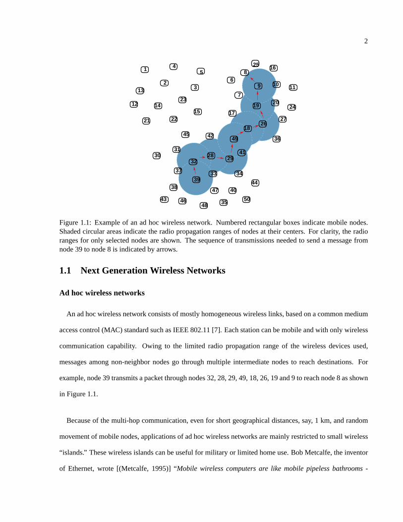
Figure 1.1: Example of an ad hoc wireless network. Numbered rectangular boxes indicate mobile nodes.Shaded circular areas indicate the radio propagation ranges of nodes at their centers. For clarity, the radioranges for only selected nodes are shown. The sequence of transmissions needed to send a message fromnode 39 to node 8 is indicated by arrows.

1.1 Next Generation Wireless Networks

Ad hoc wireless networks

An ad hoc wireless network consists of mostly homogeneous wireless links, based on a common medium

access control (MAC) standard such as IEEE 802.11 [7]. Each station can be mobile and with only wireless

communication capability. Owing to the limited radio propagation range of the wireless devices used,

messages among non-neighbor nodes go through multiple intermediate nodes to reach destinations. For

example, node 39 transmits a packet through nodes 32, 28, 29, 49, 18, 26, 19 and 9 to reach node 8 as shown

in Figure 1.1.

Because of the multi-hop communication, even for short geographical distances, say, 1 km, and random

movement of mobile nodes, applications of ad hoc wireless networks are mainly restricted to small wireless

“islands.” These wireless islands can be useful for military or limited home use. Bob Metcalfe, the inventor

of Ethernet, wrote [(Metcalfe, 1995)] “Mobile wireless computers are like mobile pipeless bathrooms -

3

78

1

2

3

4

5

9

6

10

1215

16 17

11

1314

A

B

C

D

E

F

G

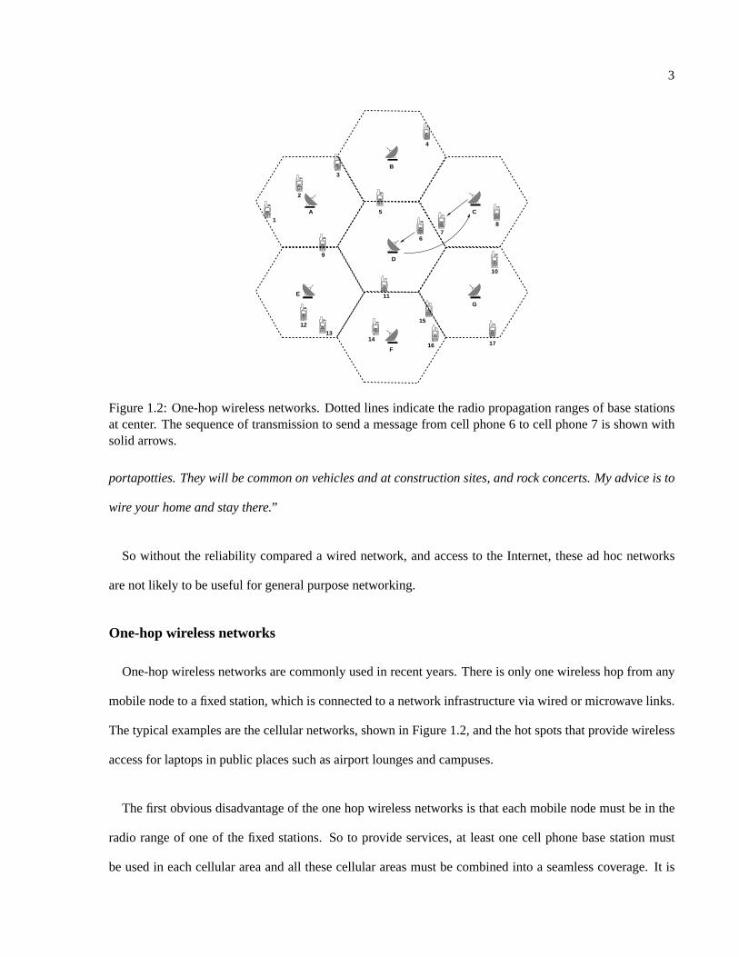
Figure 1.2: One-hop wireless networks. Dotted lines indicate the radio propagation ranges of base stationsat center. The sequence of transmission to send a message from cell phone 6 to cell phone 7 is shown withsolid arrows.

portapotties. They will be common on vehicles and at construction sites, and rock concerts. My advice is to

wire your home and stay there.”

So without the reliability compared a wired network, and access to the Internet, these ad hoc networks

are not likely to be useful for general purpose networking.

One-hop wireless networks

One-hop wireless networks are commonly used in recent years. There is only one wireless hop from any

mobile node to a fixed station, which is connected to a network infrastructure via wired or microwave links.

The typical examples are the cellular networks, shown in Figure 1.2, and the hot spots that provide wireless

access for laptops in public places such as airport lounges and campuses.

The first obvious disadvantage of the one hop wireless networks is that each mobile node must be in the

radio range of one of the fixed stations. So to provide services, at least one cell phone base station must

be used in each cellular area and all these cellular areas must be combined into a seamless coverage. It is

4

expensive and sometimes impractical to maintain these ideal cellular coverage for large areas.

The second disadvantage is the waste of time, bandwidth and energy. For example, even though cell

phones 6 and 7 in Figure 1.2 are in each other’s radio propagation range, they still have to transmit messages

to base stations D and C. Then D and C complete the path by using an infrastructure connection. With ad

hoc networking, however, phones 6 and 7 can communicate directly.

The third disadvantage is the inefficient use of resources. To avoid the “crosstalk”, the base station C and

D have to use different channels. We can’t take advantage of high shared bandwidth and have to assign for

each base station individual low bandwidth.

Mixed wired and wireless networks

Given the strengths and weaknesses of ad hoc and one-hop wireless networks, we believe that mixed

networks consisting of fixed infrastructure and mobile user nodes are suitable for a medium range network

spanning, for example, a metropolitan area; point-to-point wired or wireless links among fixed nodes and

wireless links for all nodes can be used for connectivity. These networks take advantage of both reliability

and high bandwidth of wired infrastructure backbone and flexibility and low cost of wireless links using

ad hoc networking concepts. Because these networks make use of ad hoc networking, there is no need for

fixed nodes to cover all the desired area. If a fixed node is unavailable as a neighbor, a mobile node can

send its data through other mobile nodes to the destination or to the nearest fixed node. To illustrate our

view of mixed networks, we incorporated fixed nodes with point-to-point (p2p) links among them in the

ad hoc network example shown earlier. The resulting mixed network is shown in Figure 1.3. For ease of

description, (a) we use p2p links and wired links synonymously and (b) wireless links to indicate short-haul

wireless channels among nodes.

Let us consider the communication between 39 and 8. In the mixed network, node 39 will transmit

messages to the fixed station B in its radio propagation range, and B will forward these messages to its

5

13

17

40

12

21 22

5

412930

35

18

4945

31

4

6

7

15

23

2 9

36

3

1

4648

47

32

37

38

43

28

50

44

11

26

20

27

24

25

10

816

A

14

33

C

19

B

42

39

34

Figure 1.3: Mixed wired and wireless networks. Rectangular boxes with rounded corners and numbersinside indicate mobile STAs. Diamond shape boxes with letters inside indicate fixed infrastructure nodes.Shaded circles indicate the radio propagation ranges of nodes at center. Solid lines AB, AC and BC indicatep2p links such as wired links or long-haul wireless links. All nodes are capable of using a short-haulwireless technology such as 802.16. Two sequences of transmissions are indicated. The wireless links usedare indicated by shaded circles. One is sending a message from node 39 to node 8 which use p2p linksbetween fixed infrastructure nodes B and C. The other is sending a message from node 49 to node 34 whichuse only ad hoc wireless links.

wired neighbor C. Then, these messages pass an intermediate node 9 and reach its destination node 8. This

long distance transmission involved both fixed infrastructure nodes and mobile wireless nodes. At the same

time node 49 transmits some message via wireless neighbors 41 to reach node 34. This short distance

transmission only involved wireless hops locally. These two transmissions don’t interfere with each other.

Such parallel use of wireless channels is greatly improved in mixed networks.

1.2 Designing and Using Mixed Networks

With the advent of new technologies, it is feasible to design the proposed mixed networks. The IEEE

802.11 [7] is a popular MAC protocol for ad hoc wireless networks. With a radio range of up to 376 m,

the 802.11 is a short haul wireless link protocol. The fixed infrastructure nodes are also not difficult to set

up. They can be already existing fixed nodes (access points or base stations, for example) connected via

6

p2p links. These p2p links can be wired links or long haul wireless links. For example, the new IEEE

802.16 [9] provides a long haul (less than 10 km) wireless link protocol. Recently, a few researchers have

started investigating the benefits of mixed networks [2, 21, 25].

However, there are three main challenges to using these mixed networks. First, there are no efficient

routing protocols to take advantage of both reliability and flexibility of mixed types of links. Second, many

security issues need to be solved. Third, current applications may need to be modified since the bandwidth

and quality of mixed networks may not be as good as wired networks.

1.3 Contributions of This Thesis

Our focus is on designing a routing algorithm for mixed wired and wireless networks. The current Internet

routing algorithms such as Routing Information Protocol (RIP) [18], Open Shortest Path First (OSPF) [26]

do not work well for wireless networks, while the zone routing protocol (ZRP) for ad hoc networks [17],

the cluster based routing protocol (CBRP) for ad hoc networks [19], the core extraction distributed ad hoc

routing (CEDAR) [15], associativity based routing protocol (ABR) for ad hoc networks [31], highly dynamic

destination-sequenced distance vector (DSDV) for mobile computers [27], Ad hoc On demand Distance

Vector (AODV) [28], Dynamic Source Routing (DSR) [20]and Adaptive Distance Vector (ADV) [3] focus

only on ad hoc wireless networks and do not take advantage of p2p links. The performance analysis and

comparison on several routing algorithms for ad hoc network can be found in [24, 30, 4, 14]

In this thesis, we present a new routing algorithm ADV Static (ADVS) routing algorithm, which is based

on ADV [3]. It can use specified static routes and discover and maintain any other needed routes dynam-

ically using ad hoc routing concepts. It is especially suitable for metropolitan area networks with mixed

wired and wireless links, which usually have some fixed base stations connected to the backbone of the

Internet infrastructure. ADVS routing algorithm takes into account the performance characteristics such as

bandwidth, delay and reliability of wired and wireless links and uses the existing wired network resources

as much as possible.

7

Another contribution of this thesis is implementation of ADVS in a commonly used Glomosim simulator

and enhancing Glomosim to simulate mixed networks.

To evaluate the performance benefits of mixed networks over ad hoc wireless networks, we simulated

both types of networks with ADVS as the routing protocol. We consider both UDP and TCP traffic patterns.

In all cases, mixed networks provide better throughput and packet delays. A few point to point links added

to an otherwise ad hoc network can double the throughput and halve the packet delays even when point to

point links and wireless links have the same bandwidth.

1.4 Organization

The rest of the thesis is organized as follows. Chapter 2 gives the background on the commonly used

MAC and routing protocols for MANETS. Chapter 3 introduces the Glomosim simulator and describes our

modifications to the same to facilitate simulation of mixed networks. Chapter 4 describes the ADV Static

(ADVS) routing protocol that we have developed and discusses the related design and implementation issues.

Chapter 5 presents a comparison of mixed and ad hoc networks’ performance for various types of network

traffic and different network sizes. Chapter 6 concludes the thesis.

Chapter 2

Background

We first give an overview of the MAC (medium access control) protocol used to design MANETs. Next,

we describe a few commonly used current routing algorithms for ad hoc networks. First, we define some

commonly used acronyms.

AP: Access point

BSS: Basic service set

CSMA: Carrier sense multiple access

CSMA/CA: Carrier sense multiple access/collision avoidance

CSMA/CD: Carrier sense multiple access/collision detection

DCF: Distribution coordination function

DIFS: DCF interframe space

DS: Distribution system

DSS: Distribution system service

EIFS: Extended interframe space

ESS: Extended service set

IBSS: Independent basic service set

LLC: Logical link control

MAC: Media access control

8

9

IP

TCP/ UDP

LLC

MAC

Source Host

LLC LLC

MAC MAC

Edit Host Destination Host

IP IP

TCP/ UDP

Transport Layer

LayerNetwork

Layer MAC LLC

MAC

Edit Host

IP

Figure 2.1: Protocol layer structure.

NAV: Network allocation vector

PCF: Point coordination function

PC: Point coordinator

PHY: Physical layer

SIFS: Short interframe space

STA: Station

The network protocol layer structure is shown in Figure 2.1. TCP and UDP are the commonly used

transport layer protocols. IP is the basic protocol in network layer. All routing protocols reside in network

layer and this is an active research area. There are also various standards for MAC layer protocols such

as Bluetooth [8], ultrawide band, [16], IEEE’s 802.11 [7], 802.16 [9] and 802.20 [10]. Bluetooth and

ultrawide band [16] are suitable for personal area networks since their communication range is often 10m or

less. 802.16 and 802.20 are useful for long-range wireless protocols. The 802.11 has a radio range of 100s

of meters, available inexpensively, and is suitable for battery powered devices. So it is used on the wireless

link protocol in ad hoc network designs. Since our research is based on IEEE 802.11, we will describe it

next.

10

Coordination Function

Distributed

(DCF)

Function

Coordination

Point

(PCF) ServiceContentionUsed for

Used for

FreeContention

Service

Extent MAC

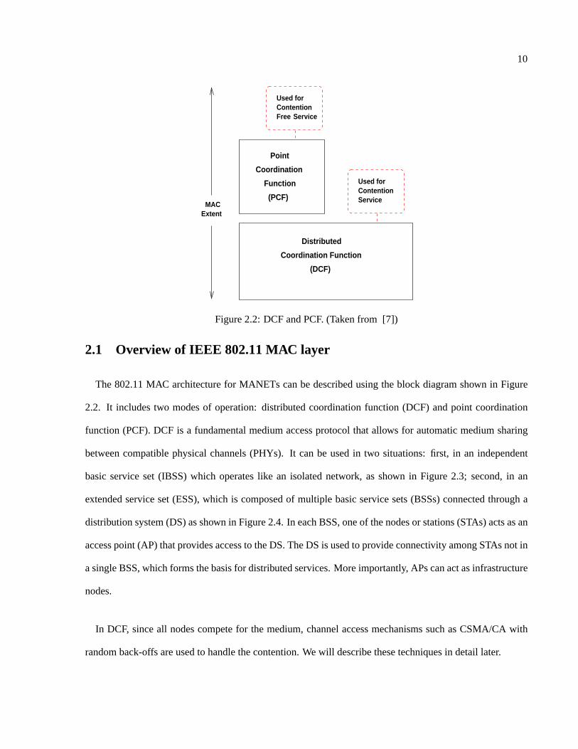
Figure 2.2: DCF and PCF. (Taken from [7])

2.1 Overview of IEEE 802.11 MAC layer

The 802.11 MAC architecture for MANETs can be described using the block diagram shown in Figure

2.2. It includes two modes of operation: distributed coordination function (DCF) and point coordination

function (PCF). DCF is a fundamental medium access protocol that allows for automatic medium sharing

between compatible physical channels (PHYs). It can be used in two situations: first, in an independent

basic service set (IBSS) which operates like an isolated network, as shown in Figure 2.3; second, in an

extended service set (ESS), which is composed of multiple basic service sets (BSSs) connected through a

distribution system (DS) as shown in Figure 2.4. In each BSS, one of the nodes or stations (STAs) acts as an

access point (AP) that provides access to the DS. The DS is used to provide connectivity among STAs not in

a single BSS, which forms the basis for distributed services. More importantly, APs can act as infrastructure

nodes.

In DCF, since all nodes compete for the medium, channel access mechanisms such as CSMA/CA with

random back-offs are used to handle the contention. We will describe these techniques in detail later.

11

802.11 ComponentsBSS 1

BSS 2

STA 1

STA 2

STA 3

STA 4

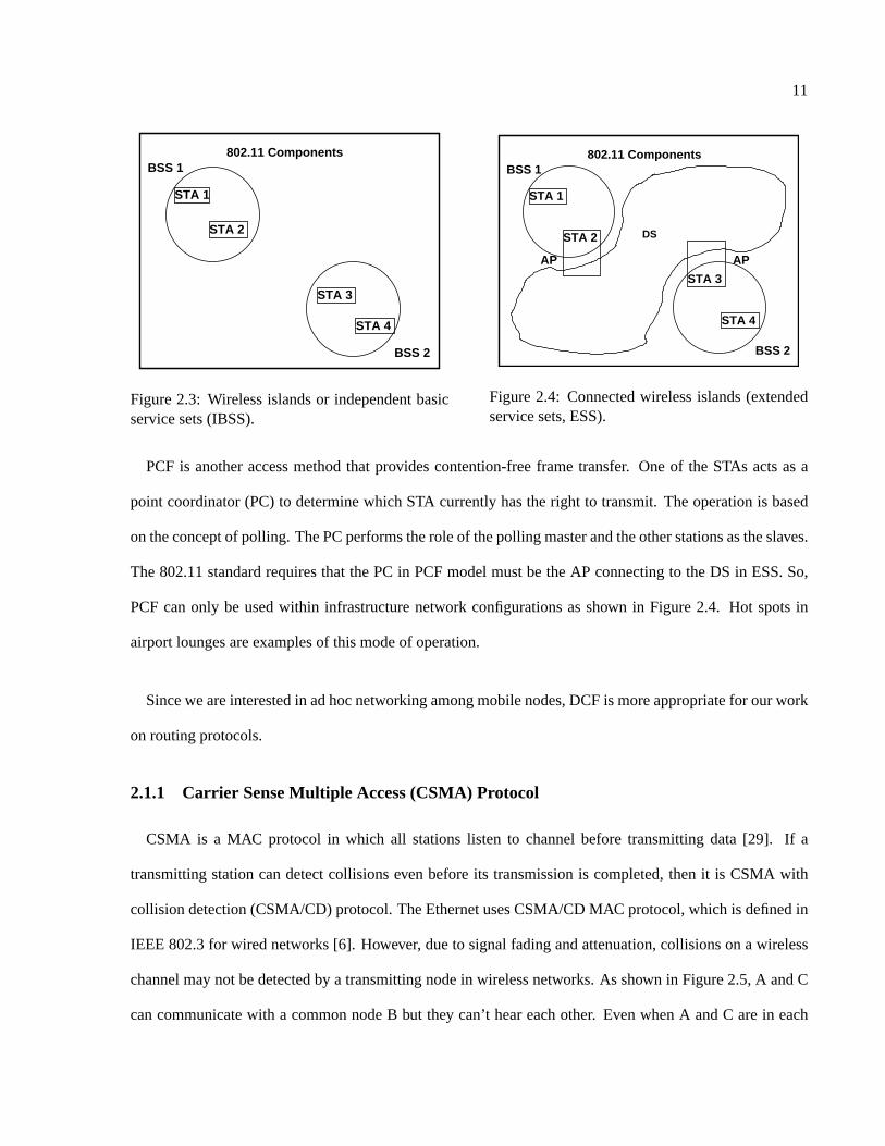
Figure 2.3: Wireless islands or independent basicservice sets (IBSS).

802.11 Components

DS

AP AP

BSS 1

STA 1

BSS 2

STA 3

STA 2

STA 4

Figure 2.4: Connected wireless islands (extendedservice sets, ESS).

PCF is another access method that provides contention-free frame transfer. One of the STAs acts as a

point coordinator (PC) to determine which STA currently has the right to transmit. The operation is based

on the concept of polling. The PC performs the role of the polling master and the other stations as the slaves.

The 802.11 standard requires that the PC in PCF model must be the AP connecting to the DS in ESS. So,

PCF can only be used within infrastructure network configurations as shown in Figure 2.4. Hot spots in

airport lounges are examples of this mode of operation.

Since we are interested in ad hoc networking among mobile nodes, DCF is more appropriate for our work

on routing protocols.

2.1.1 Carrier Sense Multiple Access (CSMA) Protocol

CSMA is a MAC protocol in which all stations listen to channel before transmitting data [29]. If a

transmitting station can detect collisions even before its transmission is completed, then it is CSMA with

collision detection (CSMA/CD) protocol. The Ethernet uses CSMA/CD MAC protocol, which is defined in

IEEE 802.3 for wired networks [6]. However, due to signal fading and attenuation, collisions on a wireless

channel may not be detected by a transmitting node in wireless networks. As shown in Figure 2.5, A and C

can communicate with a common node B but they can’t hear each other. Even when A and C are in each

12

CA B

Figure 2.5: CSMA/CA. Dotted circles indicate theradio propagation ranges of nodes at center.

A

CB

Figure 2.6: Hidden Terminal. Dotted circles indi-cate the radio propagation ranges of nodes at cen-ter. The solid black shape between node A and Cis obstacle.

other’s radio propagation range, they might not detect each other’s transmission because of the physical

obstruction as shown in Figure 2.6. In both situations, undetectable collisions can result if both two stations

believe the channel to be idle and try to transmit data to B simultaneously.

So the IEEE 802.11 uses CSMA/CA techniques to solve this problem for wireless networks. The CSMA

with collision avoidance (CSMA/CA) protocols attempt to prevent a station from transmitting simultane-

ously with other stations within its transmitting range by requiring each mobile host to ensure that the

channel is idle before transmitting. It uses the Request-to-send/Clear-to-send (RTS/CTS) exchange to re-

serve the wireless channel for transmission of a data packet. The process is as follows: (a) The sender sends

a short control packet, denoted RTS, to notify its neighbors including its intended receiver that it has data

to send. (b) If the receiver successfully received the sender’s RTS, it sends a short control packet, denoted

CTS, to notify its neighbors of pending channel use and to indicate to a sender that it is ready to receive

data. (c) The sender sends the data if it successfully receives CTS from receiver. (d) The receiver sends a

short control packet, ACK, if it receives the data successfully. The RTS/CTS exchange process is illustrated

in Figure 2.7. Both RTS and CTS frames contain a Duration/ID field that defines the period of time that

the medium is reserved for this transmission sequence. This duration field is used by the neighbor stations

to set up virtual carrier sensing. Each node maintains the network allocation vector (NAV), a record of

13

WindowContention

SIFS SIFS SIFS

DIFS

CTS ACK

Data

NAV (CTS)

NAV (RTS)

Source

Destination

Other

RTS

DIFS

Defer Access Backoff after Defer

Figure 2.7: Transmitting a data frame in 802.11. SIFS and DIFS are interframe spacings between transmis-sions. (Taken from [7].)

future traffic on the medium based on the duration information that is announced in RTS/CTS frames prior

to the actual exchange of data. 802.11 uses both virtual carrier sense mechanism (determined by NAV) and

physical carrier sense mechanism (based on the signal or noise level on the channel) to determine whether a

channel is busy.

Broadcast packets are sent only when the physical and virtual carrier senses indicate that the medium is

clear but they are not preceded by an RTS/CTS and are not acknowledged by their recipients.

The main advantage of the RTS/CTS exchange is that it performs fast collision interference and a trans-

mission path check. If the corresponding CTS is not detected by the STA originating an RTS, the originating

STA may repeat the process more quickly than if the long data frame had been transmitted and a return ACK

frame had not been detected.

The RTS/CTS exchange reserves the wireless channel for transmission of a data packet. So in the period

of the current transmission, all other STAs which can receive the RTS/CTS will think that the channel is

14

Frame

Frame

Station B

Station A

Station C

Station D

Station E

Defer

Defer

Defer

DIFS

CWindow

Backoff

CWindow

Defer

Frame

FrameCWindow

CWindow

Frame

Figure 2.8: Backoff procedure in IEEE 802.11. (Taken from [7].)

busy and execute a random back-off procedure if they also have data packets to send. To begin the back-off

procedure, the STA will set its backoff timer to a random back-off time. The backoff timer is counted down

when the channel is idle (after a DCF interframe space (DIFS) period during if the medium is determined to

be idle or the last frame is received correctly or after extended interframe space (EIFS) during if the medium

is determined to be idle or the last frame transmission was incorrect).

Randomized backoffs minimize collisions during contention between multiple STAs that have been de-

ferring to the same event. When multiple STAs are deferring and go into random back-off, then the STA

selecting the smallest back-off time will win the contention. This process is as shown in Figure 2.8.

2.2 Routing Algorithms for Ad Hoc Networks

This section will focus on the routing algorithms developed for mobile ad hoc networks. In recent years,

there are several routing algorithms designed for wireless networks. In general, they can be put into two

different groups: on-demand and proactive. The on-demand routing algorithms build or maintain only

the routing paths that have changed and are needed to send the data packets currently in the network. The

15

proactive routing algorithms disseminate routing information among all the nodes in the network irrespective

of the need for any such route. AODV [28] and DSR [20] belong to the first group. ADV [3] is a proactive

technique but exhibits some on-demand characteristics: only the existing routes are maintained and new

routes are discovered on demand.

Ad hoc On-demand Distance Vector (AODV): The Ad hoc On-demand Distance Vector routing protocol

enables multi-hop routing between participating mobile nodes wishing to establish and maintain an ad hoc

network. AODV is based on the distance vector algorithm, developed for the traditional wired network, and

treats each mobile host as a router. The basic property of distance vector routing algorithm is proactive:

each node broadcasts routing updates to its neighbors periodically or more frequently even when there is

no change in routes. However, AODV discovers a route only when needed and does not require nodes to

maintain routes to destinations that are not actively used in communications. This makes AODV an on

demand or reactive routing protocol. The needed routes are discovered using network-wide flooding of

control packets (denoted RREQs) and the replies (denoted RREPs) by target nodes. The routes discovered

are maintained in a routing table similar to that used in distance vector routing algorithm.

Dynamic Source Routing (DSR): DSR shares AODV’s on-demand characteristics in that it discovers

routes via a similar route discovery process. However, it adopts a different mechanism to store or represent

routes. A routing entry in DSR contains all the intermediate nodes to be visited by a packet rather than

just the next hop information maintained in AODV. A source puts the entire routing path in the data packet

header, and the packet is sent through the intermediate nodes specified in its header. The routing decision is

therefore made at the source. The advantage with this approach is that it is very easy to avoid routing loops.

Also the intermediate nodes need not keep routing information because the path is explicitly specified in the

data packet. The disadvantage is that packet headers are longer and of variable size.

Adaptive Distance Vector (ADV): The adaptive distance vector is a combination of proactive and on-

demand techniques. ADV shows proactive characteristics by disseminating routing information among all

16

neighbor nodes using triggered or periodic updates like in a distance vector routing protocol. It varies the

frequency and the size of the routing updates based on the network conditions.

Unlike some DV, distance vector, protocols which advertise and maintain routes for all nodes in the net-

work, ADV maintains routes to only active receivers to reduce the number of entries advertised. A node is

an active receiver if it is the receiver of any currently active connection. At the beginning of a new con-

nection, the source broadcasts (floods) network-wide with anInitconnectionadvertising that its destination

node is an active receiver. A node that receivesInitconnectionpacket marks the target ofInitconnection

as active receiver and start advertising the routes to the receiver in future updates. The target destination

node upon receiving theInitconnectionpacket responds, if it is not marked as an active receiver already,

by broadcasting network-wide with aReceiveralertpacket. Unlike the route discovery process in the on-

demand protocols, the connection-initiation process in ADV is mainly intended to advertise a destination as

an active receiver, though as a side effect the routes to the destination are also known to all nodes initially.

When a node receives such a control packet it creates an reverse path entry to the source of the control packet

in its routing table if it doesn’t have a entry to the source already. After this process, routes to the receiver

are maintained using routing updates.

ADV adaptively triggers partial and full updates such that periodic full updates are obviated. In this

protocol, a node triggers an update under three conditions: (a) if it has some buffered data packets due to

lack of routes, (b) if one or more of its neighbors make a request for fresh routes, and (c) if it is a forwarding

node that intends to advertise any fresh route to the destination so as to keep the route fresh. The impact

of all the events that require a triggered update is quantified and captured in a variable called trigger meter.

Each node keeps track of its own trigger meter. ADV adjusts the trigger meter based on the value of several

other parameters associated with the three conditions mentioned above. For example, each node categorizes

the network as HIGHSPEED or LOWSPEED based on the neighborhood changes perceived by the node.

If the number of neighbor changes is high (exceeds a certain value), then the node speed is high. Another

parameter is buffer threshold. When a new packet is buffered for lack of a route, a check is made if the

17

number of packets already buffered exceeds a preset number, called buffer threshold. If it exceeds, the

trigger meter is incremented in order to force an update. The trigger threshold is used to decide when an

update needs to be triggered. The trigger meter is reset to zero after scheduling any update. This trigger

threshold is changed dynamically based on the recent history of trigger meter values at the time of previous

partial updates. More detailed description of ADV can be found in [3, 22, 11].

Chapter 3

Glomosim Simulator

GlomoSim is a scalable wireless and wired network simulator that has been developed by Bagrodiaet

al. at UCLA [1]. It is implemented in Pasec language, suitable for parallel discrete-event simulations.

The current version of Glomosim, 2.03, has several built-in ad hoc routing protocolsand an accurate 802.11

MAC protocol. In addition, Glomosim can be used to simulate networks with point-to-point links if all

routes are specified by the user. If all routes are static, then it is feasible to simulate mixed networks.

However, Glomosim can not simulate networks with mixed p2p and wireless links if one or more routes

are incompletely specified. So Glomosim needs to be enhanced to simulate the proposed mixed networks

in which some routes are static and the rest change dynamically and need to be discovered by an ad hoc

routing protocol.

Glomosim use a layered approach based on the open system interconnect (OSI) network architecture [29].

Standard APIs are used for interaction between different simulation layers. The models currently available

in Glomosim includes:

Application: TCPLIB (telnet, ftp), CBR (constant bit rate traffic), Replicated file system, HTTP

Transport: TCP (FreeBSD), UDP, NS TCP (Tahoe) and others

Unicast Routing Protocols: AODV, DSR, Fisheye, Flooding

MAC layer: CSMA, FAMA, MACA, IEEE 802.11

Radio: Radio with and without capture capability

18

19

Mobility: Random waypoint, Random drunken, Group mobility

Glomosim is written in Parsec (a C based parallel simulation language) and includes a visualization tool

named JavaGui written in JAVA to view positions of nodes and connections among them during simulation.

We describe below a couple of modifications we made to the Glomosim simulator to facilitate simulation

and evaluation of mixed networks.

3.1 Passing information across nodes

ADVS emphasizes stable routes. Since wired links are considered to be much more stable than wireless

links, it is necessary to keep track of wireless hops and wired hops in a route. Also we need to keep track

of wired and wireless hops taken by a packet. This is easy to ensure for the control packets managed by

the routing protocol. We simply add extra variables and perform the needed updates at the routing layer. It

is much harder for data packets since this will require changes to application, or Ip header. To avoid this,

we modified the basic message structure used by Glomosim withWiredLinkCountvariable to keep track

of wired hops taken by any packet (control or data) sent over multiple hops. This new information must

be preserved when a packet is broadcasted at MAC level by a node to its neighbors, which is simulated by

duplicating the packet and providing one copy to each of the neighbors. Since the new information is added

by us, we needed go through Glomosim MAC implementation and add extra code for copying the new

information. In order to explain our modifications, which can also be used for additional statistics gathering,

we introduce the structure of Glomosim.

Glomosim has a data structure namedGlomoPartitionwhich contains the list of all nodes in this partition.

Glomosim is event-driven. The events are maintained in a heap structure.GlomoPartitionkeeps a heap for

all the nodes in the partition, so that we can easily retrieve the earliest event in this partition. When any node

creates a event, a message is formatted and inserted into the heap. The main program of Glomosim takes

the lowest time stamped event from the heap and processes it.

20

GLOMO_CallLayer

GLOMO_GetNodeData

GLOMO_SplayTreeExtractMin

GLOMO_MAC_LAYERGLOMO_RADIO_LAYER GLOMO_NETWORK_LAYER GLOMO_TRANSPORT_LAYER

GLOMO_MsgSend

GLOMO_SplayTreeInsert

1 3 // Not modified // Not modified

GLOMO_APP_LAYER

2.1 2.2

Figure 3.1: The event driven model and different protocol layers in Glomosim.

The basic structure of Glomosim is shown in Figure 3.1. The functionGLOMO SplayTreeExtractMin

extracts the message from the heap. ThenGLOMO GetNodeDatawill decide how to handle the message. If

it is a normal packet, it will be passed toGLOMO CallLayerwhich will call the appropriate layer to handle

the message. These layers include radio layer, MAC layer, network layer, transport layer and application

layer. Since our research doesn’t modify transport and application layers, we do not describe them in detail

here. We will describe the radio layer, MAC layer and network layer in detail next.

Recall the Protocol layer structure that showed in Figure 2.1. Glomosim separates the handling of wireless

and wired transmission events. To simulate a transmission over a wired link, Glomosim combines the

processing between network and MAC layers in one function. This is represented as one branch in Figure

3.2. To simulate a transmission via a wireless link, Glomosim has two branches: One handles messages that

go down from network layer to MAC layer and then down to radio layer. The other handles messages that

go up from radio layer to MAC layer and then up to network layer (see Figure 3.2).

When the network layer receives a packet from transport layer or when the MAC layer receives a packet

via wired links, theGLOMO NETWORKLAYERor theWiredLinkLayerof GLOMO MAC LAYER, respec-

tively, are called. We show in Figure 3.3 the details of branches numbered 2.2 and 3 in Figure 3.1. There are

two types of incoming packets. First, if the node is the destination of the packet, the functionProcessPack-

21

Protocol Layer Structure for Wired Transmission

Network

MAC

Protocol Layer Structure for Wireless Transmission

Network

MAC

Radio

Network

Radio

MAC

Figure 3.2: The protocol layer structure for wired and wireless transmission.

etForMeFromMacis invoked, MAC layer passes the packet up to network layer and transport layer. Second,

if the node is an intermediate node on the route to packet’s destination, the functionProcessPacketForAn-

otherFromMacis invoked, and Glomosim uses the routing algorithm in network layer to find next hop for

the packet and sends it via either wired interface or wireless interface of MAC layer. It is noteworthy that the

functionNetworkSendPacketToMacLayerinserts the packet in the queue between network layer and MAC

layer. If the packet will go out via wired interface, the functionWiredLinkNetworkLayerHasPacketToSend

will dequeue the packet and sends it to the next node. This ensures thatwiredLinkCountfield is correctly

maintained as the packet progresses.

GLOMO NETWORKLayer branch is quite similar to that forProcessPacketForAnotherFromMac. The

only difference is that the packet comes from the transport layer within the node.

When MAC layer receives a packet via wireless links,Mac80211Layerof GLOMO MAC LAYERis

called. We show in Figure 3.4 the details of the branch with number 2.1 in a cycle in Figure 3.1. After

a chain of functions, it finally generates theGLOMO RADIO StartPropagationevent to invoke the radio

22

SendToUdp SendToTcp

GLOMO_MacNetworkLayerHasPacketToSend

QueueUpIpFragmentForMacLayer

RoutingAdvTransmitData

Mac802_11NetworkLayerHasPacketToSend WiredLinkNetworkLayerHasPacketToSend

Mac802_11StartTimer

GLOMO_MsgSetLayer(msg, GLOMO_TRANSPORT_LAYER) NetworkIpSendPacketToMacLayer

NetworkIpOutputQueueDequeuePacketFifoPacketQueueDequeue

NetworkIpOutputQueueInsertFifoPacketQueueInsert

NetworkIpLayer

GLOMO_NETWORK_LAYER

GLOMO_MsgSetLayer(msg, GLOMO_MAC_LAYER)

RoutingAdvRouterFunction

RoutingAdvHandleData

ProcessPacketForMeFromMac

RouteThePacketUsingLookupTableSourceRouteThePacket

RoutePacketAndSendToMac

ProcessPacketForAnotherFromMac

ProcessPacketFromMac

NetworkIpReceivePacketFromMacLayer

WiredLinkMessageFromWire

WiredLinkLayer

GLOMO_MAC_LAYER

// wireless transmission branch// is as shown in Figure 3.4

Figure 3.3: The structure of network layer and MAC layer for wired transmission. The details of brancheswith number 2.2 in a cycle and the number 3 in a cycle in Figure 3.1 is entailed in this figure.

23

Mac802_11Layer

GLOMO_RadioStartTransmittingPacket

RadioAccnoiseStartTransmittingPacket

GLOMO_MsgSetLayer(msg, GLOMO_RADIO_LAYER)

GLOMO_MsgSetEvent(msg, GLOMO_RADIO_StartPropagation)

Mac802_11HandleTimeout

Mac802_11TransmitFrame

Mac802_11TransmitDataFrameNetworkIpOutputQueueTopPacketForAPriority

FifoPacketQueueDequeue

StartTransmittingPacket

GLOMO_MAC_LAYER

// wired transmission branch// is as shown in Figure 3.3

Figure 3.4: The structure of MAC layer for wireless transmission. This illustrates the processing done inbranches 2.2 and 3 in Figure 3.1

layer, which we explain below. In the functionMac80211TransmitDataFrame, the Glomosim dequeues the

packet stored in the queue between network layer and MAC layer. Then it allocates space for the packet to

be passed to the radio layer and copies the appropriate fields of the old packet into the new packet. So, to

pass thewiredLinkCountinformation, we added code to copy this field from old packet to each new packet

created.

The ability to keep certain book-keeping information with the packet transmitted is also useful for gather-

ing other statistics such as packet delay at routing layer. (Glomosim application layer keeps track of packet

delay at the application level, but it is cumbersome to use it and analyze it at the routing layer level.)

When the radio layer receives theGLOMO RADIO StartPropagationevent,GLOMO RADIO LAYERis

called. We show in Figure 3.5 the detail of branch 1 indicated in Figure 3.1. First,GLOMO RADIO LAYER

generates aMSGRADIO FromChannelBeginevent to notify other nodes in its radio propagation range in-

cluding the destination node. Second, after it finished the transmission, it generatesMSGRADIO SwitchToIdle

event to report the status to MAC layer. The handling ofMSGRADIO FromChannelBeginwill finally gener-

ate theMSGRADIO FromChannelEndevent and the functionGLOMO MacReceivePacketFromRadiowill

24

GLOMO_RADIO_LAYER

RadioAccnoiseLayer

GLOMO_MacReceivePacketFromRadio

event: MSG_RADIO_FromChannelEndevent: MSG_RADIO_FromChannelBegin

/* Handle arrival radio signal */

GLOMO_MsgSetLayer(msg,GLOMO_RADIO_LAYER)

GLOMO_MsgSetEvent(msg, MSG_RADIO_FromChannelEnd)

RadioAccnoiseReportStatusToMac

GLOMO_MsgSetLayer(msg,GLOMO_RADIO_LAYER)

GLOMO_PropBroadcast

GLOMO_MsgSetEvent(msg, MSG_RADIO_FromChannelBegin)

Mac802_11ReceivePacketFromRadio

Mac802_11ProcessFrame

NetworkIpReceivePacketFromMacLayer

ProcessPacketFromMac

event: MSG_RADIO_SwitchToIdleevent: MSG_RADIO_StartPropagation

GLOMO_MsgSetLayer(msg,GLOMO_RADIO_LAYER)

GLOMO_MsgSetEvent(msg, MSG_RADIO_SwitchToIdle)

ProcessPacketForMeFromMac ProcessPacketForAnotherFromMac

//The following part is completely same as the part in Figure 3.8. . . . . . . .

. . . . . . .

Figure 3.5: The structure of radio layer. This illustrates the processing done in branches 2.1 in Figure 3.1

be called to hand the packet up to MAC layer and upper network layer. The part we omitted in the figure

here is the same as that shown in Figure 3.3.

3.2 Simulating fixed and mobile nodes together

The behavior of each node in the simulation is determined by two factors. One is the mobility model and

another is the distribution model of initial positions.

To simulate our hybrid networks, we need some nodes to be fixed base stations and other nodes as mobile

users. In addition, we would like to have the ability to place fixed nodes at certain locations, while the

mobile nodes may be randomly placed based on a random distribution function. (Different scenarios can

be created by keeping everything the same and changing the seed for the random number generator used

for node placement.) But Glomosim doesn’t provide such mixed network environments. So we modified

following files to achieve this goal.

We explain the modification for mobility model first. In the fileapi.h, we add a new variablefixed to

the structureGlomoNodeto indicate whether this node is the fixed node or a mobile one. Glomosim will

read all parameters such as the number of nodes in the scenario from an input file namedconfig.inbefore

25

it starts the simulation. This field is initialized to be 0 for all nodes in the functiondriver in driver.pc.

The information of all fixed nodes is given in the file NODE-PLACEMENT-FILE, which is specified in

the parameter file config.in. In the file nodes.pc, the functionDriverGenerateInputNodes, reads the file

NODE-PLACEMENT-FILE and sets the variablefixedto be 1 for the specified fixed nodes.

With the variablefixed set correctly, we just need to design different action for fixed nodes and mo-

bile nodes in the functionGLOMO MobilityRandomWaypointWrapin mobility wrap.pc. (We modified the

builtin node mobility model random waypoint to avoid clustering of nodes unnecessarily. We call the new

model random waypoint with wraparound, which is explained in Chapter 5.) This function determine the

new position of a node once in every short interval based on node mobility. So for fixed nodes, whosefixed

value is 1, we always make the new position equal to the original position. The movement of mobile nodes

are simulated exactly as in a completely ad hoc network.

The modification of distribution model of initial positions is related with the NODE-PLACEMENT pa-

rameter in config.in. Glomosim has two models: RANDOM and UNIFORM. To accommodate mixed net-

works, we added two new models: FIXED-RANDOM and FIXED-UNIFORM. Then in the functiondriver

in driver.pc, we add two cases to handle the FIXED-RANDOM and FIXED-UNIFORM. We still use the

functionDriverGenerateRandomNodesto generate random distribution model or use the functionDriver-

GenerateUniformNodesto generate uniform distribution model for all nodes. Then we call the function

GLOMO ReadStringto read the designated positions for fixed nodes stored in NODE-PLACEMENT-FILE.

Then we replace the current positions of the fixed nodes by these designated positions.

Thus we modified the simulator to construct the mixed wired and wireless networks. To be able to

simulate large realistic mixed networks, we need a routing algorithm that can learn routes dynamically

while preserving any supplied static routes. This is described in the next chapter.

Chapter 4

A Routing Algorithm for Mixed Wired andWireless Networks

In this chapter, we describe a routing protocol for the hybrid network with both wired and wireless ca-

pability, called ADV Static (ADVS). ADVS is based on the Adaptive Distance Vector (ADV), described in

Chapter 2, and behaves like ADV for networks with only wireless links, but can utilize point-to-point links

in mixed networks to improve throughput and routing stability. In addition it will preserve any static routes

specified. We use point to point links and wired links synonymously for easier description of the protocol.

4.1 ADV Static (ADVS) Routing Algorithm

ADVS is an enhanced version of the ad hoc network routing protocol ADV described in Chapter 2. So,

ADVS uses the control packets such as InitConnection and ReceiveAlert to learn new routes and routing

updates to disseminate and maintain routes. The difference is the additional logic to take advantage of wired

links among fixed nodes. In ADVS, these control packets are broadcasted via wireless interface to inform

wireless neighbors and unicasted via wired interfaces to inform all wired neighbors. ADVS routes the data

packets the same way as ADV does. But besides considering the sequence number and cost metric of a

routing entry, ADVS uses the number of wired links in selecting routes. Thus ADVS tends to selects routes

that have fewer route breaks. In addition, mixed networks with ADVS can provide the following advantages

over ad hoc networks.

26

27

13

17

40

12

21 22

5

412930

35

18

4945

31

4

6

7

15

23

2

19

9

36

3

14

1

4648

39

47

33

32

37

38

43

34

28

42

50

44

11

26

20

27

24

25

10

816

Figure 4.1: Dissemination of routing informationin ad hoc wireless networks. The sequence of dot-ted circles from small to big indicates the propaga-tion of routing information from the source node42 through whole networks. Node 42 is the centerof all dotted circles and the process is like a ripple.

13

17

40

12

21 22

5

412930

35

18

4945

31

4

6

7

15

23

2 9

36

3

1

4648

39

47

32

37

38

43

34

28

50

44

11

26

20

27

24

25

10

816

A

14

33

C

19

B

42

Figure 4.2: Dissemination of routing informationin mixed wired and wireless networks. After theinfrastructure node B gets the routing informationfrom source 42, it transmits the same via p2p linksto A and C. Then A, B and C act as new sources ofthe routing information besides the original sourcenode 42. The sequence of dotted circles from smallto big indicates the process of transmission of rout-ing information from multiple source nodes A, Band C through whole networks. This process islike having several simultaneous smaller ripples.

Accelerate the dissemination of routing information

In ADV algorithm, the source node uses broadcasts to find routes and disseminate routing tables. Each

node that receives the information re-broadcasts it to its neighbors if the information is new. If we view the

source of the control packet at the center of co-centric rings, the dissemination of routing information is like

a ripple as shown in Figure 4.1.

In ADVS, a node sends control packets via wired interfaces by unicast before broadcasting it via the

wireless interface. Each wired neighbor will transmit the information to its wired and wireless neighbors.

So, the dissemination of routing information via wireless channels can be viewed as many ripples with

different centers as shown in Figure 4.2.

28

By placing infrastructure nodes without overlap in their radio ranges, we can accelerate the dissemination

of the routing information. Usually the bandwidth of a wired link (campus-wide: 100-1000 Mb/s, City-wide:

45-155 Mb/s) is much higher than the bandwidth of a wireless link (11-54Mb/s) and they are normally full-

duplexed. So a broadcast can be distributed among fixed nodes much more quickly compared to broadcasts

on a wireless channel. The transmission process in ADVS is like starting multiple ripples instead of the only

one increasingly larger ripples in ADV.

Decrease the delay of transmission of data

ADVS can improve packet delays significantly. We show the process of data transmission with ADV

algorithm in Figure 4.3. Assume that node 39 is trying to communicate with node 8, the transmission

depends on the intermediate nodes 32, 28, 29, 49, 13, 26, 19, 9 on the route. Recall the the CSMA/CA

MAC protocol described in Chapter 2. If any other node which is in current node’s or its nexthop’s radio

propagation range is transmitting, the current node has to wait. With more wireless nodes involved in the

route, this can cause transmission delays and reduced bandwidth to the nodes using of the wireless channel.

Usually the delay to a wired neighbor is much lower than the delay to a wireless neighbor since the

bandwidth of a wired link is much higher than the bandwidth of a wireless link and there is no contention

on point to point links. So ADVS is designed to give higher priority to p2p links in selecting routes. We

illustrate this using an example illustrated in Figure 4.3 and Figure 4.4. In the example scenario, where

node 39 is trying to communicate with node 8, the delivery of a data packet in the mixed network depends

nodes B, C and 9 on the route in order. Since it involves only three wireless transmissions, the delay to send

packets to destinations is decreased, probably significantly.

Efficient use of wireless bandwidth

ADVS makes more simultaneous transmissions feasible. Due to the CSMA/CA MAC protocol, the trans-

mission of one node on a wireless channel prevents others’ transmissions which are in the radio propagation

range of this node. For example, in Figure 4.3, when node 28 is transmitting to 29, node 32, 33, 42 have

29

������

13

17

40

12

21 22

5

412930

35

18

4945

31

4

6

7

15

23

2

19

9

36

3

14

1

4648

47

3337

38

43

34

28

42

50

44

11

26

20

27

24

25

10

816

39

32

Figure 4.3: Data transmission in ad hoc wireless networks. Dotted circles indicate the radio propagationranges of nodes at center. The sequence of transmission to send a message from node 39 to node 8 isshaded.

13

17

40

12

21 22

5

412930

35

18

4945

31

4

6

7

15

23

2 9

36

3

1

4648

47

32

37

38

43

34

28

50

44

11

26

20

27

24

25

10

816

A

14

33

C

19

B

42

39

Figure 4.4: Data transmission in mixed wired and wireless networks. Dotted circles indicate the radiopropagation ranges of nodes at center. Solid lines between AB, AC and BC indicate point to point (p2p)links such as wired links or long haul wireless links. The sequence of transmission to send a message fromnode 39 to node 8 is shaded. This transmission uses p2p links between fixed infrastructure nodes B and C.

30

to wait. So, the actual throughput achieved using wireless links can be significantly less than the specified

bandwidth. Using a few fixed infrastructure nodes and wired links, as shown in Figure 4.4, can improve the

efficiency significantly by decreasing the use of wireless channels.

Increase stability of routes

Besides higher transmission delays, another important problem in ad hoc networks is the stability of the

routes. Since most mobile nodes move randomly and quickly, a node can lose its next hop which causes

route breaks. For example, in Figure 4.3, if node 18 moves out of node 49’s radio propagation range, all the

nodes in the upper right of the figure are isolated from the rest of the network. In a mixed network, such

instances are reduced.

4.2 Implementation of ADV Static (ADVS) algorithm

4.2.1 Modifications to ADV

The code for ADVS is in file namedadvs.pcwith the corresponding definitions inadvs.h. To facilitate

simultaneous use of wired and wireless links, we define two new variables:WIRELESSMETRIC, which

denotes the metric of one wireless hop, andWIREDWIRELESSRATIO, which denotes the ratio of the band-

width of wired links to the bandwidth of wireless links. So WIRELESS METRICWIREDWIRELESS RATIO will give us the

metric of one wired link hop. We add a variablewiredLinkCountto control packetsInitconnectionandRe-

ceiveralertand also to each entry in routing updates. To select a more stable route, we use this variable to

track the number of wired links in the route from the sender of the packet to current node. In the routing

table entry, we add two variableswiredLinkCountandinterfaceIdfor the same reason.

Specifying static routes: To facilitate specification of static routes to indicate infrastructure links, ADVS

can read static routes specified in a file and put them in appropriate nodes’ routing tables. These routing

entries are not modified by the dynamic route maintenance mechanism.

31

we have modified route discovery and maintenance as follows.

Route discovery ADVS uses the route discovery process described for ADV in Chapter 2 except that it

keeps track of wired links used by control packets as they are propagated. Also, ADVS sends control packets

on both wireless and wired links.

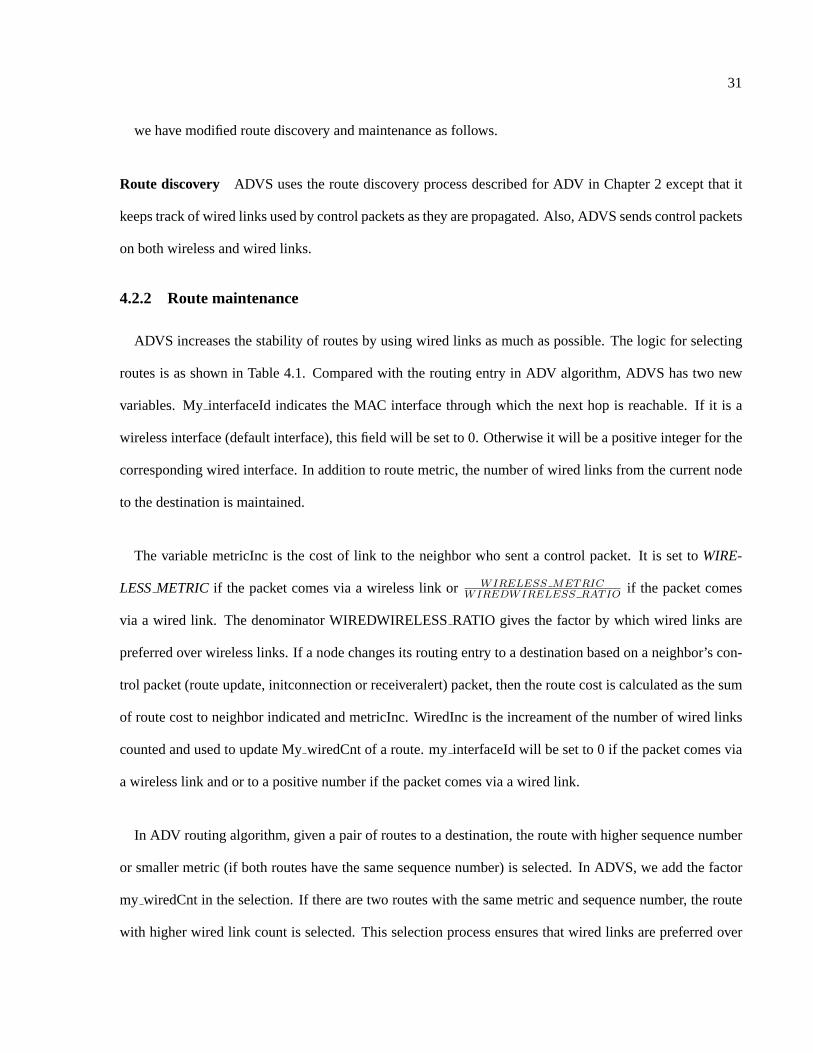
4.2.2 Route maintenance

ADVS increases the stability of routes by using wired links as much as possible. The logic for selecting

routes is as shown in Table 4.1. Compared with the routing entry in ADV algorithm, ADVS has two new

variables. MyinterfaceId indicates the MAC interface through which the next hop is reachable. If it is a

wireless interface (default interface), this field will be set to 0. Otherwise it will be a positive integer for the

corresponding wired interface. In addition to route metric, the number of wired links from the current node

to the destination is maintained.

The variable metricInc is the cost of link to the neighbor who sent a control packet. It is set toWIRE-

LESSMETRIC if the packet comes via a wireless link or WIRELESS METRICWIREDWIRELESS RATIO if the packet comes

via a wired link. The denominator WIREDWIRELESSRATIO gives the factor by which wired links are

preferred over wireless links. If a node changes its routing entry to a destination based on a neighbor’s con-

trol packet (route update, initconnection or receiveralert) packet, then the route cost is calculated as the sum

of route cost to neighbor indicated and metricInc. WiredInc is the increament of the number of wired links

counted and used to update MywiredCnt of a route. myinterfaceId will be set to 0 if the packet comes via

a wireless link and or to a positive number if the packet comes via a wired link.

In ADV routing algorithm, given a pair of routes to a destination, the route with higher sequence number

or smaller metric (if both routes have the same sequence number) is selected. In ADVS, we add the factor

my wiredCnt in the selection. If there are two routes with the same metric and sequence number, the route

with higher wired link count is selected. This selection process ensures that wired links are preferred over

32

My Entry ReceivedEntry Condition Action

Valid Valid my seqno< recv seqno Update MyEntry with Re-

ceivedEntrymy seqno == recvseqno && Update MyEntry with Re-

ceivedEntry(my metric> recv metric + metricInc||

my metric == recvmetric + metricInc &&my wiredCnt< recv wiredCnt + wiredInc)

my seqno == recvseqno && Less advertise the route.(my metric == recvmetric + meticInc &&

my wiredCnt == recvwiredCnt + wiredInc)(my seqno> recv seqno|| Set advertisement count to

help neighbors.my seqno == recvseqno &&

my metric< recv metric - metricInc)||(my seqno == recvseqno &&

my metric == recvmetric - metricInc &&my wiredCnt == recvwiredCnt + wiredInc)

Valid Invalid my seqno< recv seqno && Invalidate MyEntry since I

am dependent on thismy hop is source of this update neighbor

Set the advertisement countmy seqno>= recv seqno Set the advertisement count

recv dest == MyAddress && Set triggered updatereceiver flag == TRUE

Invalid Valid my seqno<= recv seqno Update MyEntry with Re-

ceivedEntrySet the advertisement count

my seqno> recv seqno Do nothingInvalid Invalid my seqno< recv seqno Copy recvseqno into

My Entrymy seqno> recv seqno Do nothing

Table 4.1: Processing new routing information in a control packet received. myseqno, mymetric,my interfaceId, mywiredCnt and myhop indicate the destination sequence number, hopcount, interface,and the number of wired links in the route and the next hop node currently stored in the entry forrecv dest in the routing table at the node which received this update. recvdest, recvseqno, recvmetricand recvwiredCnt indicate the values for the destination, sequence number, hop count and the number ofwired links in the route in the received routing update entry. myseqno, mymetric, and myhop indicate thedestination sequence number, hop count, and the next hop node currently stored in the entry for recvdest inthe routing table at the node which received this update. metricInc, wiredInc indicate the proper incrementof the recvmetric and wiredCnt.

33

wireless links.

Chapter 5

Performance Analysis

In this chapter, we present an analysis of mixed networks and ADVS and compare them with ad hoc

networks.

5.1 Simulation Setup

First, we describe the simulation environment.

5.1.1 Node Mobility

The Glomosim simulator has a built-in random node mobility model called random waypoint (RWP),

which is extensively used in ad hoc network simulations [13]. In RWP model, each node begins the sim-

ulation by remaining stationary for specified seconds, called the pause time, which can be set to 0. Then

it selects a random geographical destination in the simulated field. It moves to the destination at a speed

randomly selected between minimum and maximum specified node speeds. Upon reaching the geographical

destination, the node pauses again for the specified amount of pause time. This behavior is repeated for the

duration of the simulation. The RWP model has two disadvantages. If the geographical destination is not in

the field, the node will reselect a new destination. This is repeated until a geographical destination within

the field is selected. This causes all mobile nodes to move toward the center of the square with higher prob-

ability, which results in clustering of majority of nodes in the middle of the field. Another disadvantage is if

a node’s speed is chosen to be very low or 0 m/s, it could stay at that speed for the remainder of simulation.

34

35

So the average node speed tends to decrease with time if the minimum node speed is 0 m/s [32].

We modified the RWP model slightly to address the problem of clustering in the middle of the field. In our

model, a node may choose a geographical destination that is outside the field. If a node reaches the boundary

of a field, it reenters the field immediately from the other (parallel) side of the field with the same speed and

direction and completes the remaining distance. We call this RWP with wraparound model. We also choose

a random speed for node movement to vary between 1 m/s and 29 m/s (108Km/hr). This mitigates the

second disadvantage of RWP. We simulated only continuous node mobility with 0-second pause times.

5.1.2 Types of Links

We used two types of links for simulations. One type is the wireless link whose bandwidth is 2 Mb/s with

a radio range of 376 m. This is consistent with the 802.11 protocol implemented in Glomosim. The other

type is a point-to-point (p2p) link. This can be a wired or long haul wireless link based on, for example,

IEEE 802.16. Since wired links are supported by Glomosim, we used wired links with 2 Mb/s bandwidth,

2.5 µsec propagation delay and full-duplex capability as the p2p links among infrastructure nodes. We

limited the bandwidth of wired links to 2 Mb/s to show that even with such low bandwidth, mixed networks

can outperform ad hoc wireless networks significantly. For route selection purposes, we set the wired link

to wireless link ratio,r, to 10. Based on our experience and several published results [5], an ad hoc network

with 50-100 nodes and several simultaneous connections in a 1.5 to 2.5 sq. km area typically achieves a

throughput of about 1/5th of maximum wireless channel BW (2 Mbps in our simulations) for UDP traffic,

while a point-to-point link can achieve throughput very close to its nominal BW. Since we use full duplex

p2p links and half-duplex wireless links, a ratio of 10 seemed appropriate.

5.1.3 Types of Networks

We simulated small (50-nodes in a1.5×1.5 Km2 field) and large (1000 nodes in a6×6 Km2 field) ad hoc

and mixed networks. We simulated three types of small networks: (a) 50 mobile nodes with only wireless

capability (Figure 5.1), (b) 50 mobile nodes and additional 9 fixed nodes, with only wireless capability

36

22

30

15

23

11

25

42

45

31

17

7

1500 m

1500 m

12

3548

4643

3839

44

4047

33 34

413629

37

32

49

2726

1821

14

1920

24

28

910

86

5

3213

4 16

1

0

Figure 5.1: Fifty-node wireless network in a field of 1500m x 1500m. Rectangular boxes with roundedcorners and numbers inside indicate mobile nodes.

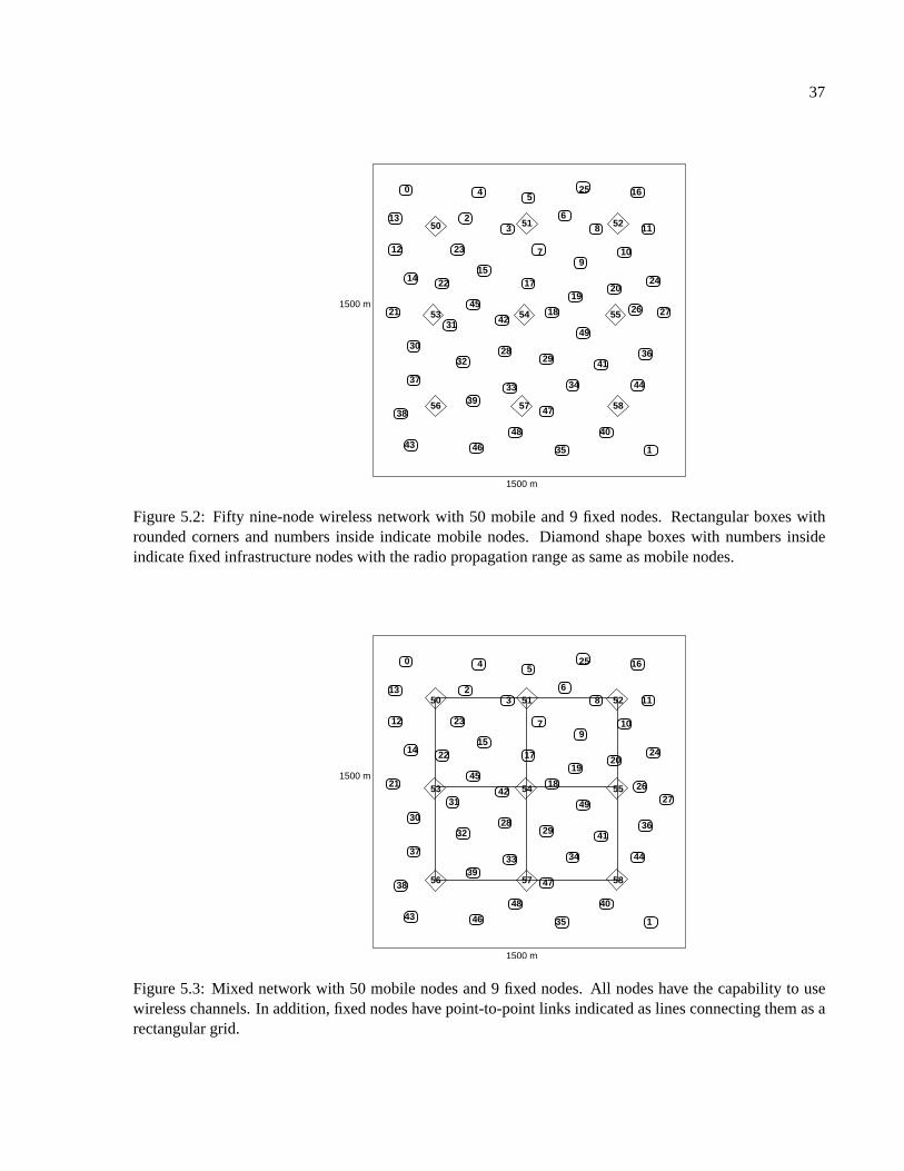
(Figure 5.2), and (c) 50 mobile nodes with wireless capability and 9 fixed nodes with wireless capability

and 12 wired links among them (Figure 5.3). The 9 fixed nodes form a3× 3 grid in the middle of the field.

The distance between adjacent fixed infrastructure nodes is 500m. So they can not communicate with one

another directly with wireless links. We simulated three large networks: (a) 1000 mobiles nodes with only

wireless capability; (b) 991 mobile nodes, 9 fixed nodes with wireless capability and 12 p2p links among

them; and (c) 975 mobiles and 25 fixed nodes with wireless capability and 40 p2p links. In both small and

large networks, we ensured that fixed nodes are neither source nor destination nodes.

As explained in chapter 3, we modified Glomosim simulator so that a specified list of stationary nodes

can be placed at predetermined locations, while the remaining nodes are placed randomly in the field with

the specified mobility model.

5.1.4 Traffic Models

We used UDP and TCP traffic patterns to evaluate mixed networks and ADVS . We used constant bit rate

(CBR) to simulate UDP traffic and HTTP and FTP to simulate TCP traffic. We vary the network load for

the case of CBR traffic by varying the packet rates of 25 CBR connections. The packet size is fixed at 512

37

22

30

15

23

11

25

42

45

31

17

7

1500 m

1500 m

12

48

4643

39

44

47

33 34

413629

37

32

49

271821

14

1920

24

28

910

86

5

32

4 16

26

38

40

35

13

0

50

1

51 52

53 54 55

56 57 58

Figure 5.2: Fifty nine-node wireless network with 50 mobile and 9 fixed nodes. Rectangular boxes withrounded corners and numbers inside indicate mobile nodes. Diamond shape boxes with numbers insideindicate fixed infrastructure nodes with the radio propagation range as same as mobile nodes.

22

30

15

23

11

25

42

45

17

7

1500 m

1500 m

12

48

4643

39

44

47

33 34

413629

37

32

49

1821

14

1920

24

28

910

86

5

32

4 16

38

13

40

35

2726

31

50

1

0

51 52

53 54 55

56 57 58

Figure 5.3: Mixed network with 50 mobile nodes and 9 fixed nodes. All nodes have the capability to usewireless channels. In addition, fixed nodes have point-to-point links indicated as lines connecting them as arectangular grid.

38

bytes. We vary the network load for TCP traffic by varying the number of HTTP and FTP connections.

HTTP traffic is generated using the built-in Glomosim model, which is based on the Zipf law [23].

For small networks, 10 scenarios are generated with different random mobile node placements at the

start of simulation. Each data point presented here is an average of 10 such simulations. This minimizes

any skewing of results based on a particularly good or bad scenario. For large networks, each data point

presented here is an average of 5 simulations. Each simulation is run for 600 seconds.

5.1.5 Routing protocols

We implemented ADVS in Glomosim. We used ADVS for all types of networks. For ad hoc wireless

networks, ADVS is the same as ADV. In addition, we also simulated AODV routing protocol for ad hoc

wireless networks (distributed with Glomosim code) to illustrate that the results obtained with ADV are rep-

resentative of the performance achievable in wireless ad hoc networks. So any performance improvements

by ADVS in mixed networks are clearly due to the use of p2p links.

5.1.6 Static Routes

Glomosim lets static route specification and usage when a dynamic routing protocol is not used. Because

of this, when static route option is used, all possible routes need to be specified, and the routes cannot change

during the simulation. This is not feasible with mobile nodes. So we implemented ADVS such that it can

read wired links with which two nodes are connected specified in a file and put them in appropriate nodes’

routing tables. The static p2p links do not fail and are not modified by the dynamic route maintenance

mechanism. Each p2p link indicates a 1-hop static route between the nodes it connects.

5.1.7 Metrics and Parameters

We used following metrics to evaluate the routing protocols and networks:

• Throughput:The total amount of data (in Kb/s) delivered to the destinations.

39

• Average packet latency:The time, in milliseconds, it takes for a data packet to reach its destination

from the time it is generated at the source and includes all the queuing and protocol processing delays

in addition to propagation and transmission delays.

• Routing Overhead on wireless links (pkts/s):The number of routing packets transmitted per second by

the routing layer to MAC layer. For packets sent over multiple hops, each transmission of the packet

(each hop) counts as one transmission. This is the routing overhead seen at the routing layer level.

We also examined secondary metrics such as MAC layer network allocation vector, which indicates chan-

nel contention, hop counts, and the rate of broken routes to illustrate the reasons for performance differences

among routing protocols and networks.

5.2 Small Ad Hoc Networks

ADVS is used to denote ADVS routing protocol in the 59-node mixed network and ADV 50 and ADV 59

are used to denote ADV in 50-node and 59-node wireless networks, respectively. AODV 50 indicates the

performance of AODV for the 50-node wireless network. The 25 CBR connections simulated use nodes 0-

24 as senders and nodes 25-49 as destinations. To avoid using senders or destinations as fixed nodes, which

could skew the results in favor of mixed networks, we have used 9 separate nodes as fixed infrastructure

nodes in the small ad hoc network case. For this reason we simulated a 59-node mixed network. To show

that adding 9 extra nodes without p2p links is not beneficial, we also simulated a 59-node wireless network

with 50 mobile and 9 fixed nodes.

5.2.1 UDP traffic

First, we evaluate the networks using UDP traffic, which is simulated using 25 CBR connections and the

size of each packet is 512 bytes. Figure 5.4 give the throughputs of ADVS, ADV 59, ADV 50 and AODV

50. Figure 5.5 gives the corresponding delivery rates, where a delivery rate is the fraction of the injected

packets that were delivered to destinations.

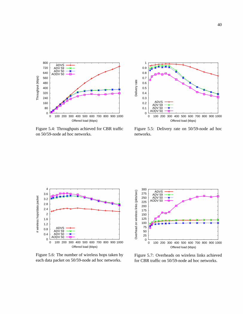
40

0

80

160

240

320

400

480

560

640

720

800

0 100 200 300 400 500 600 700 800 900 1000

Thr

ough

put (

kbps

)

Offered load (kbps)

ADVSADV 59ADV 50

AODV 50

Figure 5.4: Throughputs achieved for CBR trafficon 50/59-node ad hoc networks.

0

0.1

0.2

0.3

0.4

0.5

0.6

0.7

0.8

0.9

1

0 100 200 300 400 500 600 700 800 900 1000

Del

iver

y ra

te

Offered load (kbps)

ADVSADV 59ADV 50

AODV 50

Figure 5.5: Delivery rate on 50/59-node ad hocnetworks.

0

0.4

0.8

1.2

1.6

2

2.4

2.8

3.2

3.6

4

0 100 200 300 400 500 600 700 800 900 1000

# w

irele

ss h

ops/

data

pac

ket

Offered load (kbps)

ADVSADV 59ADV 50

AODV 50

Figure 5.6: The number of wireless hops taken byeach data packet on 50/59-node ad hoc networks.

0 25 50 75

100 125 150 175 200 225 250 275 300

0 100 200 300 400 500 600 700 800 900 1000

Ove

rhea

d on

wire

less

link

s (p

kts/

sec)

Offered load (kbps)

ADVSADV 59ADV 50

AODV 50

Figure 5.7: Overheads on wireless links achievedfor CBR traffic on 50/59-node ad hoc networks.

41

We notice in Figure 5.4 that the maximum throughput achieved with ad hoc wireless networks is 380

Kb/s. In the mixed network, the max throughput is 750 Kb/s, nearly twice as much. Since ADV 59 and

ADVS have the same number of mobile and fixed nodes, it is clear that the increase in performance is due to

p2p links. To understand the reasons for this increase in performance, we examined the number of wireless

hops taken by data packets. Figure 5.6 shows that the average number of wireless hops taken by a delivered

packet in mixed networks is around 2.35 and that for wireless networks with ADV 50, ADV 59 or AODV is

about 3.22. So the load placed on wireless links is reduced by3.22−2.352.35 = 37%. This accounts for some of

the throughput increase we observed.

The rest of the improvement in throughput with p2p links is due to two factors: (a) less interference

of transmission on wireless links because fewer wireless links used by a data packet; (b) ADVS reduces

the probability of broken routes and provides more stable routes by using wired links as much as possible.

To show that p2p links reduce interference on wireless channels significantly, we examined the network

allocation vector (NAV) at the MAC layer. This NAV indicates the duration wireless channel is reserved at

any instant of time; smaller NAV means reduced contention. We sampled NAV each time MAC protocol

needs to transmit a packet and calculated the average NAV. Figure 5.8 presents the average NAV observed

for various protocols and networks. The average NAV is indicative of the network performance before

the network is saturated (Beyond saturation, NAV does not indicate network performance properly due to

frequent broken routes and increased use of channel BW for control packets.) Based on this we see that

the average NAV for mixed network is about 50% smaller than that of the wireless networks. To examine

the second factor, we calculated the rate of route breaks in each type of network. The rate of broken routes

is shown in Figure 5.9. Mixed network has much fewer broken routes than the wireless networks. It is

particularly interesting to compare ADV and ADVS. The rate of broken routes increases rapidly for loads

beyond 300 Kbps for ADV, while it is more gradual for ADVS. AODV has a higher rate of broken routes

prior to saturation; this rate is bounded in saturation because it takes more time to repair routes compared to

other algorithms and most routes stay broken for extended periods of time.

42

0

4e-05

8e-05

0.00012

0.00016

0.0002

0.00024

0.00028

0.00032

0.00036

0.0004

0 100 200 300 400 500 600 700 800 900 1000

Ave

rage

NA

V

Offered load (kbps)

ADVSADV 59ADV 50

AODV 50

Figure 5.8: Average Network Allocation Vec-tor(NAV) on 50/59-node ad hoc networks.

0 5

10 15 20 25 30 35 40 45 50 55 60

0 100 200 300 400 500 600 700 800 900 1000

Bro

ken

rout

es/s

econ

d

Offered load (kbps)

ADVSADV 59ADV 50

AODV 50

Figure 5.9: Average broken routes on 50/59-nodead hoc networks.

0

400

800

1200

1600

2000

2400

2800

3200

3600

4000

0 100 200 300 400 500 600 700 800 900 1000

Ave

rage

del

ay (

ms)

Offered load (kbps)

ADVSADV 59ADV 50

AODV 50

Figure 5.10: Average delays achieved for CBRtraffic on 50/59-node ad hoc networks.

0

50

100

150

200

250

300

350

400

450

500

0 40 80 120 160 200 240 280 320 360 400

Ave

rage

del

ay (

ms)

Offered load (kbps)

ADVSADV 59ADV 50

AODV 50

Figure 5.11: Average delays (offerloads from 0 to80 kbps) achieved for CBR traffic on 50/59-nodead hoc networks.

It is noteworthy that even though the wired link bandwidth is 2 Mb/s, adding 12 p2p links nearly doubles

the throughput. If we use wired links with higher bandwidth, the throughput will be improved even further.

Figure 5.10 gives average packet delays. At low to moderate loads (less than 150 kbps), all networks have

comparable delays. As the load increases, the wireless networks saturate and packet delays grow rapidly.

However, the mixed network saturates at higher loads and packet latencies do not grows as fast as in the

other networks. Figure 5.11 gives an enlarged view of packet delays prior to saturation. This figure shows

loads varying from 0 to 400 kbps. It is clear that even in uncongested networks, mixed network provides

lower latencies.

43

0

50

100

150

200

250

300

350

400

450

500

0 5 10 15 20 25

Thr

ough

put (

kbps

)

HTTP connections

ADVSADV 59ADV 50

AODV 50

Figure 5.12: Throughputs achieved for HTTP traf-fic on 50/59-node ad hoc networks. Each serverhas one client.

0

50

100

150

200

250

300

350

400

450

500

0 5 10 15 20 25

Thr

ough

put (

kbps

)

HTTP connections

ADVSADV 59ADV 50

AODV 50

Figure 5.13: Throughputs achieved for HTTP traf-fic on 50/59-node ad hoc networks. Each serverhas three clients.

Figure 5.7 gives the CBR traffic overheads for the three networks. We notice that the overheads of ADVS,

ADV 59 and ADV 50 are nearly constant as the offered load increases. But AODV has significantly higher

overhead owing to its on demand approach of discovering and maintaining routes. Routing algorithms such

as ADV which control the number of control packets tends to perform better in congested networks.

5.2.2 TCP traffic

We have simulated TCP traffic using HTTP and FTP applications. In Figure 5.12, we show the throughput

achieved for the case where HTTP server serves one client. Figure 5.13 shows the throughput achieved for

the case when each server has three clients. Comparing these two figures, we find that the performance of

AODV drops slightly with the increase in the number of servers. ADV 50 and ADV 59 perform similarly

indicating that the infrastructure nodes by themselves do not improve performance. ADVS gives signifi-

cantly higher throughput (50% more) compared to ADV 50 and ADV 59. AODV underperforms ADV in

most instances.

Figure 5.14 and Figure 5.15 show the overheads of two HTTP configurations. In both cases, with the

increase in the number of connections, the overheads of ADV 50, ADV 59 and ADVS reach a maximum

value and do not exceed this value since the ADV algorithm limits update packets to 2 per second per

44

0

20

40

60

80

100

120

140

160

180

200

0 5 10 15 20 25

Ove

rhea

d on

wire

less

link

s (p

kts/

sec)

HTTP connections

ADVSADV 59ADV 50

AODV 50

Figure 5.14: Overheads on wireless links achievedfor HTTP traffic on 50/59-node ad hoc networks.Each server has one client.

0

20

40

60

80

100

120

140

160

180

200

0 5 10 15 20 25

Ove

rhea

d on

wire

less

link

s (p

kts/

sec)

HTTP connections

ADVSADV 59ADV 50

AODV 50

Figure 5.15: Overheads on wireless links achievedfor HTTP traffic on 50/59-node ad hoc networks.Each server has three clients.

0

120

240

360

480

600

720

840

960

1080

1200

0 5 10 15 20 25

Thr

ough

put (

kbps

)

FTP connections

ADVSADV 59ADV 50

AODV 50

Figure 5.16: Throughputs achieved for FTP trafficon 50/59-node ad hoc networks.

0

20

40

60

80

100

120

140

160

180

200

0 5 10 15 20 25

Ove

rhea

d on

wire

less

link

s (p

kts/

sec)

FTP connections

ADVSADV 59ADV 50

AODV 50

Figure 5.17: Overheads achieved for FTP traffic on50/59-node ad hoc networks.

node. But the overhead of AODV increases with the increase in number of connections, primarily due to

maintaining routes individually.

Figure 5.16 gives throughputs of various networks for FTP traffic. With the increase in the number of

connections, the throughput advantage of mixed network over other networks decreases. TCP uses backoff

when the network is congested and uses available bandwidth as much as possible. So, in ad hoc networks,

TCP performs better than UDP [12]. Since an FTP connection has infinite amount of data to transmit and the

available bandwidth of wired links has already been used as much as possible, even with a few connections,

the additional throughput realized with increased number of connections is reduced. Figure 5.17 give the

45

0

250

500

750

1000

1250

1500

1750

2000

2250

2500

0 300 600 900 1200 1500 1800 2100 2400 2700 3000

Thr

ough

put (

kbps

)

Offered load (kbps)

ADVS25FADVS9F

ADVAODV

Figure 5.18: Throughputs achieved for CBR trafficon 1000-node ad hoc networks.

0

0.1

0.2

0.3

0.4

0.5

0.6

0.7

0.8

0.9

1

0 300 600 900 1200 1500 1800 2100 2400 2700 3000

Del

iver

y ra

te

Offered load (kbps)

ADVS25FADVS9F

ADVAODV

Figure 5.19: Delivery rates for CBR traffic on1000-node ad hoc networks.

FTP traffic overheads which are similar to those seen for HTTP traffic.

To summarize our results for small networks, we note that the throughputs and average delays achieved

by ADV 59 are almost the same as those by ADV 50. That is because the 9 fixed nodes in ADV 59 have

only wireless capability and just act as intermediate nodes. But we can achieve significant improvement in

performance by adding wired point-to-point links among infrastructure nodes.

5.3 Large Ad Hoc Networks

ADVS25F denotes ADVS routing protocol in a 1000-node network with 25 fixed nodes and ADVS9F

the same for 1000-node network with 9 fixed nodes. ADV and AODV are used to denote ADV and AODV

routing protocols in networks with 1000 mobile nodes.

UDP traffic

We evaluate the networks using UDP traffic, which is simulated using 25 CBR connections sending 512-

byte packets. Figures 5.18 and 5.19 give the CBR traffic throughputs and delivery rates of ADVS25F,

ADVS9F, ADV and AODV.

46

The maximum throughput achieved with ad hoc wireless networks using ADV routing protocol is 835

kb/s. In the mixed network, the max throughput of ADVS9F is 1359 kb/s, 63% higher, and that of ADVS25F

is 2421 Kb/, 190% higher. Once again mixed networks provide significantly higher performance for similar

reasons: lower wireless channel contention (given in Figure 5.22), reduced number of wireless hops (shown

in Figure 5.20), and fewer broken routes (given in Figure 5.23). What is noteworthy, however, is that the

performance is improved with only a few fixed nodes and p2p links in the large network. The number of

fixed nodes is a small percentage (0.9 to 2.5%) of the total number of nodes. (In contrast, the number of

fixed nodes is 15% of the total nodes in the 59-node mixed network.) The number of p2p links used is 12

with 9 fixed nodes or 40 with 25 fixed nodes. Yet the performance improvement is even higher than that

seen for smaller networks.

Figure 5.20 show that the average number of wireless hops taken by a delivered packet. When the offered

load is 2000 Kb/s, the mixed network with 9 fixed nodes delivers a throughput of 1315 Kb/s with an average

of 6.9 wireless hops per delivered data packet. In contrast, the ad hoc network with no fixed nodes delivers

a throughput of 778 Kb/s with an average of 9.4 hops (all hops are wireless in this network) per delivered

data packet. So9.4−6.96.9 = 36% wireless hops are saved by adding 12 extra wired links. This accounts for

some of the 57% throughput increase we observed. Since in large ad hoc networks, each route involves

more wireless hops and is broken more easily, ADVS25F improves the performance even more since more

mobile nodes can directly access fixed nodes. The performances of ADV and AODV illustrate why pure ad

hoc networks can only be useful in small areas.

As shown in Figure 5.19, among the ad hoc protocols, ADV is able to perform adequately achieving 70%

or higher delivery rates prior to saturation and peak throughput of 835 Kbps. AODV does not perform well

and saturates much more quickly with a peak throughput of 608 Kbps. Even at low loads, its delivery rate is

less than 56%.

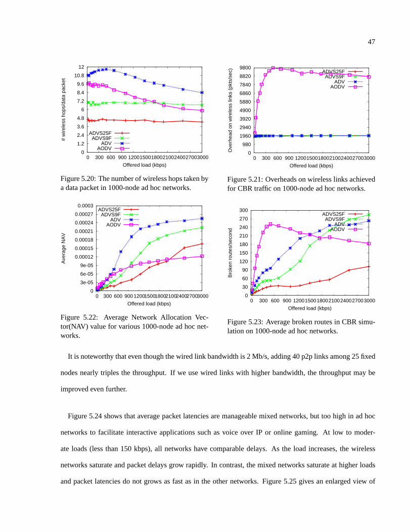
47

0

1.2

2.4

3.6

4.8

6

7.2

8.4

9.6

10.8

12

0 300 600 900 1200 1500 1800 2100 2400 2700 3000

# w

irele

ss h

ops/

data

pac

ket

Offered load (kbps)

ADVS25FADVS9F

ADVAODV

Figure 5.20: The number of wireless hops taken bya data packet in 1000-node ad hoc networks.

0

980

1960

2940

3920

4900

5880

6860

7840

8820

9800

0 300 600 900 1200 1500 1800 2100 2400 2700 3000

Ove

rhea

d on

wire

less

link

s (p

kts/

sec)

Offered load (kbps)

ADVS25FADVS9F

ADVAODV

Figure 5.21: Overheads on wireless links achievedfor CBR traffic on 1000-node ad hoc networks.

0

3e-05

6e-05

9e-05

0.00012

0.00015

0.00018

0.00021

0.00024

0.00027

0.0003

0 300 600 900 1200 1500 1800 2100 2400 2700 3000

Ave

rage

NA

V

Offered load (kbps)

ADVS25FADVS9F

ADVAODV

Figure 5.22: Average Network Allocation Vec-tor(NAV) value for various 1000-node ad hoc net-works.

0

30

60

90

120

150

180

210

240

270

300

0 300 600 900 1200 1500 1800 2100 2400 2700 3000

Bro

ken

rout

es/s

econ

d

Offered load (kbps)

ADVS25FADVS9F

ADVAODV

Figure 5.23: Average broken routes in CBR simu-lation on 1000-node ad hoc networks.

It is noteworthy that even though the wired link bandwidth is 2 Mb/s, adding 40 p2p links among 25 fixed

nodes nearly triples the throughput. If we use wired links with higher bandwidth, the throughput may be

improved even further.

Figure 5.24 shows that average packet latencies are manageable mixed networks, but too high in ad hoc

networks to facilitate interactive applications such as voice over IP or online gaming. At low to moder-

ate loads (less than 150 kbps), all networks have comparable delays. As the load increases, the wireless

networks saturate and packet delays grow rapidly. In contrast, the mixed networks saturate at higher loads

and packet latencies do not grows as fast as in the other networks. Figure 5.25 gives an enlarged view of

48

0

350

700

1050

1400

1750

2100

2450

2800

3150

3500

0 300 600 900 1200 1500 1800 2100 2400 2700 3000

Ave

rage

del

ay (

ms)

Offered load (kbps)

ADVS25FADVS9F

ADVAODV

Figure 5.24: Average delays achieved for CBRtraffic on 1000-node ad hoc networks.

0

20

40

60

80

100

120

140

160

180

200

0 50 100 150 200 250 300 350 400 450 500

Ave

rage

del

ay (

ms)

Offered load (kbps)

ADVS25FADVS9F

ADVAODV

Figure 5.25: Average delays (offerloads from 0 to500 kbps) achieved for CBR traffic on 1000-nodead hoc networks.

packet delays prior to saturation. This figure shows loads varying from 0 to 500 kbps. It is clear that even in

uncongested networks, mixed network provides lower latencies.

Figure 5.21 gives the CBR traffic overheads for the three networks. We notice that overheads with

ADVS25F, ADVS9F and ADV are nearly constant as the offered load increases. But AODV has significantly

higher overhead owing to its on demand approach of discovering and maintaining routes.

5.3.1 TCP Traffic

We have simulated TCP traffic using varying number of HTTP connections. Figure 5.26 shows the

throughput achieved for the case where each HTTP server serves five clients. Figure 5.27 shows the through-

put achieved for the case when each server has 10 clients.

It is noteworthy that the throughput goes up by almost 5 times in the mixed networks. We get even more

throughput improvement for HTTP than CBR since HTTP is based on TCP which makes connections before

transmission. The reliable route can keep the connection alive for even longer and reduce the overhead to

build connections. Since infrastructure nodes provide more reliable routes, the need for route discovery for

each HTTP session is reduced.

49

0

100

200

300

400

500

600

700

800

900

1000

0 10 20 30 40 50

Thr

ough

put (

kbps

)

HTTP connections

ADVS25FADVS9F

ADVAODV

Figure 5.26: Throughputs achieved for HTTP traf-fic on 1000-node ad hoc networks. Each server hasfive clients.

0

90

180

270

360

450

540

630

720

810

900

0 10 20 30 40 50

Thr

ough

put (

kbps

)

HTTP connections

ADVS25FADVS9F

ADVAODV

Figure 5.27: Throughputs achieved for HTTP traf-fic on 1000-node ad hoc networks. Each server hasten clients.

Chapter 6

Conclusions

With the advent of ad hoc wireless networks, there are more and more demands on them to take advantage

of the flexibility and provide easy access to the Internet, but still have the stable and high performance

characteristics of the traditional wired networks. We have proposed mixed networks that are primarily

ad hoc wireless networks with some fixed nodes with p2p links added to provide better performance and

reliability. Recently a few other researchers also started investigating mixed networks [2, 21, 4].

It is feasible to deploy the proposed mixed networks inexpensively. The IEEE 802.11 is a popular MAC

protocol for ad hoc wireless networks as a short-haul wireless link protocol. The p2p links among infrastruc-

ture nodes can be wired links or long haul wireless links such as IEEE 802.16 wireless link protocol. The

infrastructure nodes can even be already existing fixed nodes connected via p2p links (for example, access

points connected to the Internet). Or these to could be semi-permanent nodes that remain stationary for a

few hours and have p2p links implemented via a suitable wireless technology, for example, IEEE 802.16.

We proposed a routing algorithm, denoted ADVS, that can work well in ad hoc networks as well as mixed

networks we proposed. We implemented ADVS in the Glomosim simulator. Also, we modified Glomosim

to simulate mixed networks.

We have shown using simulations that mixed networks perform significantly better than ad hoc networks.

For UDP and TCP traffic, mixed networks can provide significantly higher throughput and lower packet

50

51

delays. We simulated a large ad hoc network with 1000 nodes in a 36 Km2 area to see the practicality of ad

hoc networking in a reasonably large geographical region. While pure ad hoc networks are unusable, adding

a few infrastructure nodes with p2p links offers high throughput and low delays.

Future work

In future, we would like to evaluate mixed networks and ADVS using real time video applications. An-

other interesting topic to explore is optimal placement of fixed nodes and links and possibly using multiple

wireless channels by fixed nodes. We also would like use 802.16 based wireless links instead of wired links

as point-to-point links among infrastructure nodes. We are also interested in robust low overhead security

protocols that take advantage of the infrastructure nodes in mixed networks to facilitate authentication and

key management.

Bibliography

[1] R Bagrodia et al. Glomosim: A scalable network simulation environment, v2.03. Parallel ComputingLab, UC Los Angeles, CA. http://pcl.cs.ucla.edu/projects/glomosim, December 2000.

[2] P. Bhagwat, B. Raman, and D. Sanghi. Turning 802.11 inside-out. InProceedings of HotNets-II, 2003.

[3] R. V. Boppana and S. P. Konduru. An adaptive distance vector routing algorithm for mobile, ad hocnetworks. InProceedings of IEEE Infocom, April 2001.

[4] S. R. Das, R. Castaneda, and J. Yan. Simulation based performance evaluation of mobile, ad hocnetwork routing protocols. InSeventh Int’l Conf. on Computer Communication and Networks, 1998.

[5] S. R. Das, C. E. Perkins, and E. M. Royer. Performance comparison of two on-demand routing proto-cols for ad hoc networks. InProceedings of IEEE Infocom 2000, March 2000.

[6] IEEE Standards Department. IEEE 802.3 standard for local area networks – carrier sense multipleaccess with collision detection (CSMA/CD) access method and physical layer specifications, 1985.

[7] IEEE Standards Department. IEEE 802.11 standard for wireless LAN, medium access control (MAC)and physical layer (PHY) specifications, 1997.

[8] IEEE Standards Department. IEEE Bluetooth standard: Wireless mac and phy specifications for wire-less personal area networks, 1997.

[9] IEEE Standards Department. IEEE 802.16 standard: Wirelessman standard for broadband wirelessmetropolitan area networks, 2004.

[10] IEEE Standards Department. IEEE 802.20 standard: Mobile broadband wireless access (MBWA),2004.

[11] T. D. Dyer. Design and Analysis of Adaptive Routing and Transport Protocols in Mobile Ad HocNetworks. PhD thesis, The University of Texas at San Antonio, 2002.

[12] T. D. Dyer and R. V. Boppana. A comparison of TCP performance over three routing protocols formobile ad hoc networks. InProceedings of ACM Mobihoc, October 2001.

[13] J. Broch et al. A performance comparison of multi-hop wireless ad hoc network routing protocols. InProceedings of ACM Mobicom’98, Oct. 1998.

[14] P. Johansson et al. Scenario-based performance analysis of routing protocols for mobile ad hoc net-works. InProceedings of ACM Mobicom, 1999.

52

53

[15] R. Sivakumar et al. Cedar: Core extraction distributed ad hoc routing.IEEE Journal on Selected Areasin Communication, Special Issue on Ad hoc Networks, pages Vol 17, No.8, 1999.

[16] J. Foerster, E. Green, S. Somayazulu, and D. Leeper. Ultrawide band technology for short or mediumrange wireless communications.Intel Technology Journal, pages vol. 5, no. 2, 2001.

[17] Z. J. Haas and M. R. Pearlman. The zone routing protocol (zrp) for ad hoc networks.IETF InternetDraft, draft-ietf-zone-zrp-00.txt, 1997.

[18] C. Hedrick. Routing information protocol.Internet RFC 1058, 1988.

[19] M. Jiang, J. Li, and Y.C. Tay. The cluster based routing protocol (cbrp) for ad hoc networks.IETFInternet Draft, draft-ietf-manet-cbrp-spec-01.txt, 1999.

[20] David B Johnson and David A Maltz. The dynamic source routing in ad hoc wireless networks. InInternet Draft, draft-ietf-manet-dsr-03.txt, 1999.

[21] R. Karrer, A. Sabharwal, and E. Knightly. Enabling large-scale wireless broadband: The case for taps.In Proceedings of HotNets-II, 2003.

[22] S. P. Konduru. An adaptive distance vector routing algorithm for mobile, ad hoc networks. Master’sthesis, The University of Texas at San Antonio, 2000.

[23] L.Breslau, P.Cao, L.Fan, G.Phillips, and S.Shenker. Web caching and zipf-like distributions: evidenceand implications. InProceedings of INFOCOM’99 (IEEE Press), 2000.

[24] S. Lee, Mario Gerla, and C. K. Toh. A simulation study of table-driven and on-demand routing proto-cols for mobile ad hoc networks.IEEE Network Magazine, August 1999.

[25] S. Mehra and C. Yu. Enhancing the performance of mobile ad hoc networks with the aid of internetgateways. InICWN 2004 International Conference, 2004.

[26] J. Moy. Ospf version 2. InInternet RFC 1583, March 1994.

[27] C. E. Perins and P. Bhagwat. Highly dynamic destination-sequenced distance vector (dsdv) for mobilecomputers. InProceedings of ACM SIGCOMM’94, pages 234–244, 1994.

[28] C. E. Perkins, E. M. Moyer, and S. R. Das. Ad hoc on demand distance vector (AODV) routing.IETF,Internet Draft, IEEE RFC 3561, http://www.ietf.org/rfc/rfc3561.txt?number=3561, July 2003.

[29] Peterson and Davie.Computer Networks: A systems approach, volume 3rd edition. Morgan Kaufmann,2003.

[30] E. Royer and C. K. Toh. A review of current routing protocols for ad hoc mobile wireless networks.IEEE Personal Communications Magazine, pages Vol 6, No.2, April 1999.

[31] C. Toh. Associativity based routing protocol (abr) for ad hoc networks.IETF Internet Draft, draft-ietf-manet-longlived-adhoc-routing-00.txt, 1999.

[32] J. Yoon, M. Liu, and B. Noble. Random waypoint considered harmful.IEEE INFOCOM, 2003.

Vita

Zhi Zheng was born in Xin Jiang, China on June 12, 1978, the son of Jingren Zheng and Lianrui Du.

In 2001, he graduated from Beijing University of Posts and Telecommunications, receiving the Bachelor of

Engineering with a major in Computer Science . He entered the graduate program at UTSA in 2002.

He can be reached attylerzheng@yahoo.com.

Publications in Computer Science

R.V. Boppana and Z.Zheng, ”Improving Performance of Wireless Ad Hoc Networks Using a Few Point-

to-Point Links.”, Wireless Network Communications Group(WCNG) Symposium, 2004.

R.V. Boppana and Z.Zheng, ”On the Performance of Wireless Metropolitan Area Networks.”, in the

Proceedings of IEEE Wireless Communications and Networking Conference (WCNC), 2005.

R.V. Boppana and Z.Zheng, ”Designing Ad Hoc Networks with Limited Infrastructure Support.”, in the

Proceedings of IEEE Wireless Consumer Communications and Networking Conference (CCNC) , 2005

54