Routing and Staffing in Large Call Centers withSpecialized and Fully Flexible Servers

Philippe ChevalierUniversité catholique de Louvain, chevalier@poms.ucl.ac.be

Robert A. ShumskyUniversity of Rochester, shumsky@simon.rochester.edu

Nathalie TabordonBelgacom Mobile/Proximus, nathalie.tabordon@proximus.net

Initial version: March, 2004. Latest revision: June, 2004

AbstractWe use models of loss systems and a queueing simulation to optimize routing and

staffing decisions in large call centers with any number of customer types and a mixtureof dedicated and completely flexible servers. Given that flexible servers are no fasterthan specialists for a particular customer type, we show that in the loss system it isalways optimal to send customers to specialists first. If all appropriate specialists arebusy, we show that it is always optimal to send the customer to a flexible server, as longas the service time distribution on the flexible server is independent of the customertype. To specify the optimal mixture of dedicated and flexible staff, we find that asimple 80/20 rule works well for a remarkably wide range of parameters. In particu-lar, for call centers that provide excellent service by setting a tight constraint on thecustomer loss rate or average waiting time, we find that 20% of the staffing budgetshould be spent on flexible servers while 80% should be spent on dedicated servers.We provide some intuition as to why a single proportional solution is so robust anddiscuss extensions to other types of systems.

Keywords: call centers, capacity flexibility, queueing networks, routing.

1 Introduction

An international call center outsourcer provides customer service, inbound sales, and tech-

nical support for three corporate clients. During business hours this call center staffs over

1

300 agents, most of whom provide support for the customers of a single client company.

However, the outsourcer has also trained a select group of “super-reps” who can handle calls

for all three clients. Because of their training and skills, the super-reps are more expensive

than the regular staff, but the firm argues that the capacity flexibility provided by these

cross-trained servers is worth the cost. In general, most call centers handle calls requiring a

variety of skills, and many call centers have arranged their staffs into configurations similar

to this outsourcer: groups of dedicated servers and a group of cross-trained servers to provide

some flexibility.

When using this configuration, a call center must answer two basic questions: (i) how

many specialist and cross-trained servers should be deployed? and (ii) given a particular

staffing level, when should a call be routed to a dedicated or a cross-trained server? Our

goal here is to provide general answers to these questions for large call centers. By ‘large,’

we mean call centers with over 40, and perhaps hundreds, of servers, and with offered loads

from each customer type equivalent to at least 20.servers. Our interest in large call centers

follows from industry trends. According to one study, the average call center in 2001

employed approximately 50 customer service agents (Ewalt, 2003), and it is not unusual to

find call centers with as many as 500 agents (Mitchell, 2001). In addition, for much of

this paper we focus on high-quality call centers that either aim to provide excellent service

(in terms of loss rates or the wait in queue) so that significant queues rarely form, or have

extremely impatient customers. Examples include premium-class call centers for banks or

airlines, call centers for emergency services, or business environments in which the caller pays

a significant surcharge for the connection. Our primary results are derived from a stochastic

model of a loss system in which customers who find all servers busy leave the system, and

we then test our results using a simulation of a queueing system.

For loss systems, the intuitive solution to question (ii) is the correct solution: calls should

be sent to a dedicated server if one is available, while cross-trained, or ‘flexible’ servers, should

2

be held in reserve. The answer to question (i) can depend upon the arrival, capacity and

cost parameters of the call center, but here we use a numerical approximation to show that

a simple 80/20 rule works well for a remarkably wide range of parameters. For high-quality

call centers, we find that 20% of the staffing budget should be spent on flexible servers

while 80% should be spent on dedicated servers. In a thorough series of numerical tests,

the performance of this heuristic is almost always superior to either ‘extreme’ solution (all-

specialized or all-flexible servers) and often performs nearly as well as the globally optimal

solution. Of course, the 80/20 rule is not optimal for all parameters. It is obvious that if

flexibility is costless then an all-flexible system is preferable, while for call centers offering

low-quality service (high loss rates or a relatively long wait in queue) an all-specialist system

is almost always nearly optimal. However, for high-quality call centers, the 80/20 staffing

is an excellent heuristic for most reasonable parameters, and it can be useful for aggregate

staff planning over long time horizons or as a starting point for more precise optimization

using detailed simulation.

We review the literature in the next section. Section 3 presents the basic model, Section

4 describes results on optimal call routing, and Section 5 describes the approximation we

use to find the optimal staffing configuration for a loss system. Sections 6 and 7 focus on

the optimization problem. Section 6 reports on the relative effectiveness of the 80/20 rule

for symmetric systems in which all customers have equal arrival and service rates, while

Section 7 describes a variety of alternative parameters and an alternative formulation of

the optimization problem. This section also describes the queueing simulation and the

performance of the heuristic when customers who find a busy system are not lost. Section

8 concludes with a summary of our findings and a description of future research.

2 Related Literature

Previous work on call-center staffing has focused primarily on systems with homogeneous

servers. An exhaustive survey by Gans, Koole and Mandelbaum (2003) traces the ‘square-

3

root staffing principle’ back to the work of Erlang in the 1920’s. More recently the rule has

emerged from a variety of queueing and staffing models, including those of Whitt (1992) and

Borst, Mandelbaum and Reimann (2004). Armony and Maglaras (2001, 2002) extend the

square-root principle to systems with two types of customers, those who desire immediate

service and those who are willing to accept a ‘call-back’ option. Garnett, Mandelbaum and

Reiman (2002) extend this principle to the case where customers have a stochastic reneging

time. In all of these papers, there is a single pool of servers with identical skills.

The literature on skill-based routing in call centers is also summarized in Gans et al.

(2003), and Hopp and van Oyen (2003) present a literature survey and research taxonomy

for cross-training in more general production settings. The system described in this paper

has pools of specialists and a pool of fully cross-trained servers, and therefore is an example

of the ‘M system’ described in Garnett and Mandelbaum (2001). In these systems, some

servers can only see a subset of customers, and the staffing problem is much more complex

than for systems with homogeneous servers. As the article by Gans et al. (2003) points

out, the staffing decision in a system with nonhomogeneous servers is intertwined with the

lower-level routing problem: which available server should a newly-arrived customer choose,

and which available customer should a newly-free server select? For this reason, much recent

work has focused on the dynamic routing problem in which the routing decision depends

upon the states of the queues and servers, e.g., see Gans and van Ryzin (1997) and Harrison

and López (1999) for heavy-traffic analyses of the problem. Iravani and Krishnamurthy

(2002) focus on finite-source queueing systems, e.g., the repairman problem. They allow for

an arbitrary mix of specialized and partially cross-trained servers and examine numerically

the performance of a variety of repairman-assignment rules. Borst and Seri (2000) propose

a routing heuristic that assigns customers to the available agent with the most specialized

set of skills, a generalization of the ‘specialist-first’ routing described below.

Örmeci (2002) analyzes a system with two types of calls and three pools of operators,

two dedicated and one cross-trained. The system described by Örmeci is both more general

4

than ours (different customer types may offer different rewards) and more restrictive (there

are two customer types). The article shows that it is optimal to serve a call with a dedicated

operator if one is available. If a dedicated server is not available, then there exist conditions

on the arrival rates, service times, and reward values that indicate whether it is always

optimal to send a customer to the cross-trained pool. Below, we extend certain results from

Örmeci (2002) to systems with more than two types of calls.

Another class of papers focus on performance evaluation, cross-training, and staffing

problems. Green (1985), Stanford and Grassmann (1993), and Shumsky (2003) analyze

systems with single pools of flexible and specialized servers (an ‘N’ system, using the termi-

nology of Garnett and Mandelbaum, 2001). Stolletz (2003, chapter 5) examines an M-system

with limited waiting space, customer balking, and reneging. Borst and Seri (2002) describe

a general cross-training scheme and develop sufficient conditions on the number of servers

of each type needed to satisfy given performance constraints. They also derive a set of

necessary conditions. For the system described in this paper, Borst and Seri’s sufficient

and necessary conditions for the total number of servers are equivalent to the bounds im-

plied by the two extreme cases: a system with only specialists and a system with all servers

fully cross-trained. Harrison and Zeevi (2003) use a stochastic fluid model to find optimal

long-run staffing configurations in large call centers with cross-training, under the assump-

tion that variations in the average arrival rate dominates short-term fluctuations around the

mean.

Other authors approximate the performance of more general queueing systems by limiting

the waiting-space (Gurumurthi and Benjaafar, 2001), by deriving bounds on the performance

(Aksin and Karaesmen, 2002) or by assuming that all servers are either specialized or fully

cross-trained (Agnihothri, 2003). In much of this paper (until Section 7.4), we assume that

there is an infinite customer population arriving to a loss system: if a customer finds all

the appropriate specialized servers and all the flexible servers busy, then that customer must

leave the system. Both Koole and Talim (2000) and Chevalier and Tabordon (2003) develop

5

performance evaluation methods for loss systems with general topologies.

The earlier papers by Green and by Stanford and Grassmann focused on methodology,

i.e., matrix-geometric methods for performance assessment. The more recent papers aim

to generate qualitative insights into the value of cross-training. Shumsky (2003) describes

the trade-off between the lower cost of dedicated servers and the flexibility of cross-trained

servers. Both Aksin and Karaesmen (2002) and Gurumurthi and Benjaafar (2001) examine

the value of a variety of cross-training schemes, including the value of server flexibility in both

symmetric and asymmetric systems, where a ‘symmetric system’ has the same arrival rate

and available capacity for each customer type. Using very different models, both find that

in asymmetric systems, more server flexibility does not necessarily lead to higher customer

throughput. Chakravarthy and Agnihothri (2003) and Agnihothri et. al. (2003) use numer-

ical methods and simulation, respectively, to evaluate the benefits of flexibility in queueing

systems similar to the one described here. While their system includes waiting-lines, they

focus on relatively small systems (up to 20 servers) with two customer types. Numerical

experiments in Stolletz (2003) also focus on systems with approximately 20 servers. These

experiments demonstrate how the optimal percentage of generalist servers is sensitive to a

variety of parameters, including the service rate of the generalists and their cost premium.

Finally, Wallace and Whitt (2004) examine systems with many customer types (e.g., six)

and an arbitrary cross-training matrix. They use heuristics and simulation to find the min-

imum number of cross-trained servers needed to satisfy performance goals for each customer

type. Their experiments demonstrate that most of the benefits of full cross-training can be

achieved by cross-training each server with just two skills.

In fact, many of these papers point out that ‘a little flexibility goes a long way.’ For

the system considered here, most of the benefits of flexibility are provided by a few flexible

servers. However, the optimum level of flexibility declines as the cost of cross-training

increases. Our goal is to generate specific guidelines for estimating the optimum number of

fully cross-trained servers for large call centers handling many types of calls.

6

3 The Loss Model

We assume that there are multiple customer types, each arrives according to a Poisson

process, and that all service times are distributed as independent, exponential random vari-

ables. For each type of customer there may be a pool of specialist servers, and there may

also be a separate pool of flexible servers who are able to handle any customer type, perhaps

at a lower service rate. The system is described by the following parameters:

M : number of customer types.

λi: arrival rate of type-i customers (i = 1...M).

µi: specialist’s service rate of a type-i customer.

ni: number of specialists who handle type-i customers.

µfi : flexible server’s service rate for a type-i customer.

nf : number of flexible servers.

Again, we assume that the call center is a loss system: customers who do not find a

specialist or flexible server available are lost. For the optimization problem described in

Section 6, we will specify a maximum system-wide loss rate, Ψ(n1, . . . , nM , nf) and will seek

to minimize the staffing cost, and in Section 7.1 we discuss the problem of minimizing the

loss rate, given an upper bound on the staffing costs. In Section 7.4 we present numerical

results that will help us to associate these loss probabilities with the performance measures

of a queueing system.

To specify the staffing costs we first normalize staffing wages and benefits so that the

expense per unit time of a specialist is ‘1’. We also assume that each additional skill

acquired by a flexible server has a cost premium of p, so that the cost per unit time of a

fully flexible server is 1+(M−1)p. For example, a call center for a European bank employscustomer service agents who speak up to four different languages (Dutch, English, French

7

and German). Managers at this bank estimate that the additional cost of a cross-trained

employee is 5% per language, so that p = 0.05.

4 Optimal Routing

In the call-center literature, specialist-first routing schemes are often assumed to be optimal

for systems with specialists and completely cross-trained servers (e.g., Agnihothri et al.,

2003; Stolletz, 2003). By using coupling arguments, Örmeci (2002) demonstrates that this

routing scheme is optimal for loss systems with two call types, and in the following theorem

we show that optimality also holds for our loss system withM call types. Moreover, Örmeci

(2002) defines conditions under which it is optimal to send a call to a flexible server when

no specialist is available. In Corollary 1, below, we find that if all customers have the same

service rate when assigned to a flexible server, then, again, no customers should be turned

away. When there are two call types, our results reduce to a particular case of the notion of

preferred classes, as defined in the article by Örmeci. Proofs are included in the Appendix.

Theorem 1 If µfi ≤ µi, i = 1...M , then it is optimal to route an arriving customer to a

specialist if one is available.

The proof formulates the problem as an undiscounted Markov Decision process and uses

value iteration to show that sending a customer to a specialist brings a higher expected

reward than using a cross-trained operator and that a policy maximizing the utilization of

the specialists is optimal.

Corollary 1 If µfi = µf , µf ≤ µi, i = 1...M , and no specialist is available, then it is optimal

to route an arriving customer to a flexible server if one is available.

The proof of the corollary also uses value iteration for this particular case, to show that

it is always optimal to increase the utilization of cross-trained servers.

Note that if µfi < µfj for some i, j, then it may sometimes be optimal to reject a type-i

customer when a flexible server is available, with the hope that a quicker type-j customer

8

may come along soon. Given that there are two customer classes, Örmeci (2002) describes a

state-dependent threshold rule for accepting a customer for service. However, in the following

sections we assume that all calls follow the ‘specialist-first’ routing and that calls are never

rejected if any server is available. Again, this routing policy is optimal when µfi = µfj for

all i, j, and is consistent with the routing policies found in most call centers.

5 An Approximation Based on Hayward’s Method

To determine the loss rate Ψ(n1, . . . , nM , nf), we might use numerical methods to find for the

steady-state behavior of a Markov-chain representation of the system. However, the exact

performance of many systems of this size cannot be evaluated numerically. For example,

Stolletz (2003, pg. 106) points out that the Markov matrix describing an M-system with

limited waiting space (a system similar to ours) can require a state space with over 1 million

states when there are 100 servers, 15 million states when there are 200 servers, and 7 billion

states when there are 1000 servers, Simulation is an alternative, and we will use simulation

in Section 7.4, but again, lengthy run-times are required to generate reliable estimates of

output parameters, and the run-times increase as the system size increases.

Here we propose an approximation procedure based on Hayward’s method (Fredericks,

1980) and developed in Tarbordon (2002). This approximation has three advantages over

numerical methods to find the ‘exact’ performance. First, it is extremely fast and is scal-

able. The computational requirement for performance evaluation in systems with hundreds

of servers is not significantly larger than for systems with just a few servers, so that loss

rates can always be found in a fraction of a second. Second, the system interpolates perfor-

mance results between integer servers. This allows us to use efficient numerical methods for

solving optimization problems, and enables us to see general patterns and trends without

the distortions that occur when the system is restricted to an integral number of servers.

Third, the approximation is extremely accurate for many parameter ranges, and is always

sufficiently accurate for our purposes (more on its accuracy, below).

9

The approximation requires three steps. First, compute the overflow from each pool

of dedicated servers. Second, merge the overflows from the dedicated pools to form the

arrival stream to the fully cross-trained operators. Third, compute the overflow at the fully

cross-trained pool and the overall loss probability of the call center. To begin, let B(n, ρ)

be Erlang’s loss function, given n servers and an offered load of ρ. Because we will allow

for a non-integral number of servers, we use the following interpolation of Erlang’s function,

proposed by Jagerman (1984) :

B(n, ρ) =

·ρ−neρ

Z ∞

ρ

e−yyndy¸−1

(1)

Note that the integral from ρ to ∞ is sometimes defined as the incomplete gamma function

and that B(n, ρ) is exactly equal to Erlang’s function when n is an integer. Let ρi = λi/µi,

so that the rate of overflow from each pool of specialists to the pool of flexible servers is

νi = λiB(ni, ρi) (2)

and let ρ0i = νi/µi.

Hayward’s approximation describes the stream of arrivals to the flexible pool in terms

of both the average arrival rates (νi) and the ‘peakedness’ of the arrivals. The peakedness

is a measure of the variability of the flow, and is defined as the ratio of (i) the variance in

the number of servers needed to serve all calls (assuming an M/G/∞ queue) and (ii) the

average number of servers needed to serve all calls. In particular, from Fredericks (1980),

the peakedness of the overflow from a single pool is

zi = 1− ρ0i +

ρini − ρi + ρ

0i + 1

. (3)

Because the pool of flexible servers sees overflows from allM pools of specialized servers,

it sees an average arrival rate λf =PM

i=1 νi and an offered load ρf = λf/µf . Following

Hayward’s method, we then approximate the peakedness of the flexible pool’s arrival stream

as

10

zf =1

λf

MXi=1

νizi. (4)

and the overall loss probability is

Ψ(n1, ...nM , nf) =

λfB(nf

zf, ρ

f

zf)PM

i=1 λi. (5)

Numerous studies have shown that the first two moments of an arrival stream, the arrival

rate and the peakedness, are often sufficient to compute reasonably accurate approximations

of the performance of loss networks (see, for example, the comparisons in Fredericks, 1980,

Guerin and Lien, 1990, and Tabordon, 2002). To supplement these results, we used both

simulation and numerical techniques to make three types of comparisons between results

obtained from the approximation and the performance of the actual system. In particular,

we compared the approximation and the actual system using (i) the calculated loss rates,

(ii) the optimal number of cross-trained servers, and (iii) the performance of our staffing

heuristics (as described in the next section). All of these experiments demonstrated that

for the large systems of interest here - those with 50 servers or more - the approximation

is extremely accurate. These results are consistent with Whitt (1984), who uses a heavy-

traffic approximation of the blocking probability to show that Hayward’s approximation

should perform well in systems with heavy loads. In the interest of brevity, we do not

present the results of comparisons (i) and (ii) here, although details are available from the

authors. We will summarize the results of the third set of comparisons at the end of the

next section.

6 Optimal Staffing for a Symmetric System: the 80/20

Rule

In this section we restrict our attention to systems in which all customers have the same

arrival rates (λi = λj = λ) and all service rates are independent of both the customer type

11

and the server type (µi = µj = µfi = µfj = µ). If there are dedicated servers, then it is

optimal to staff the same number of dedicated servers, n, for each customer type. Define

Ψ(n, nf) as the loss probability for a system with M pools of n dedicated servers, and one

pool of nf flexible servers. We consider the following optimization problem, that minimizes

cost subject to a constraint on the overall loss probability:

minn,nf

Mn+ (1 + (M − 1)p)nf (6)

s.t. Ψ(n, nf) ≤ Ln ≥ 0, nf ≥ 0.

By using the approximation described above to calculate Ψ, we found the optimal values of

n and nf for a variety of values for the exogenous parameters. In particular, we assumed a

normalized service rate (µ = 1) and we varied λ from 10 to 80, M from 2 to 5, the target

loss rate L from 0.01 to 0.2, and p from 0 to 0.25. This covers a wide range of call centers.

For example, the total load on the call center, Mλ, varies from 20 to 400 and the total cost

premium of a cross-trained server, 1 + (M − 1)p, varies from 0 to 100%.

Certain conclusions from the experiments are obvious, e.g., the optimal number of cross-

trained servers declines as p rises. However, we found that the optimal percentage of the

total budget spent on cross-trained servers, (1 + (M − 1)p)nf/ £Mn+ (1 + (M − 1)p)nf¤,at first declines rapidly as p rises, but then reaches a level that is relatively flat over a wide

range of p. For example, Figure 1 shows this plateau for M = 2, L = 0.01, and the entire

range of λ. Figure 2 shows a similar effect with L = 0.01, M = 2, 3, 4 and 5, and λ adjusted

for each value of M so thatMλ = 100. Figure 3 displays the optimum solution withM = 2

and λ = 20, while L varies. We noted that the plateau is often close to 0.2, and therefore

we proposed a ‘80/20 rule’: spend 80% of the budget on specialists and 20% of the budget

on cross-trained servers.

12

1

0.8

0.6

0.4

0.2

0.05 0.1 0.15 0.2 0.25Cross-training premium (p)

Opt

imal

fract

ion

ofbu

dget

spen

ton

cros

s-tra

ined

serv

ers

λ = 10

λ = 20

λ = 40

λ = 80

Figure 1: Optimal fraction of budget spent on cross-trained servers for systems with L = 0.01

and M = 2.

1

0.8

0.6

0.4

0.2

0.05 0.1 0.15 0.2 0.25Cross-training premium (p)

Opt

imal

fract

ion

ofbu

dget

spen

ton

cros

s-tra

ined

serv

ers

M = 2

M = 3

M = 4

M = 5

Figure 2: Optimal fraction of budget spent on cross-trained servers for systems with L = 0.01

and Mλ = 100.

13

Loss probability = 0.01

Loss probability = 0.05

Loss probability = 0.1

Loss probability = 0.2

Cross-training premium (p)

Opt

imal

fract

ion

ofbu

dget

spen

ton

cros

s-tra

ined

serv

ers

0.05 0.1 0.15 0.2 0.25

1

0.8

0.6

0.4

0.2

Figure 3: Optimal fraction of budget spent on cross-trained servers for systems with M = 2

and λ = 20.

This is certainly not an ‘exact’ result - the true optimum is 100% when p is very small,

or 0% when p and L are large, as is true when L = 0.2 in Figure 3. However, there are wide

parameter ranges over which the 80/20 rule is either close to the optimum, or, if not close,

performs well in terms of cost despite being sub-optimal. Figure 4 was generated using

L = 0.01, λ = 20, andM = 2, and the figure shows the cost penalty, the percentage increase

in the objective-function value under the 80/20 rule when compared with the true minimum

value from the optimization problem (6). We see that the cost penalty when using the ‘rule

of thumb’ is never greater than 2% and is often close to zero. On the same graph we see the

cost penalty of the best extreme solution is substantially higher for all but the very lowest

values of p (in this instance, an all-flexible configuration is the best extreme solution over

the range 0 ≤ p ≤ 0.125, and an all-specialist configuration is the best extreme solution forhigher values of p).

However, we also find that when L is high the 80/20 rule can perform poorly when

compared to the best extreme solution. Figure 5 shows the cost penalty, as in Figure 4,

but with L = 0.2 rather than 0.01. In this case, an all-specialist system is the preferred

14

0 0.05 0.1 0.15 0.2 0.250

0.01

0.02

0.03

0.04

0.05

0.06

0.07

0.08

0.09

cross-training premium (p)

% a

bove

opt

imum

cos

t

20% heuristicBest extreme solution

0 0.05 0.1 0.15 0.2 0.250

0.01

0.02

0.03

0.04

0.05

0.06

0.07

0.08

0.09

cross-training premium (p)

% a

bove

opt

imum

cos

t

20% heuristicBest extreme solution

Figure 4: Percentage above optimum cost for the 80/20 rule and the best extreme solution,

with L = 0.01, M = 2, and λ = 20.

0 0.05 0.1 0.15 0.2 0.250

0.005

0.01

0.015

0.02

0.025

0.03

0.035

cross-training premium (p)

% a

bove

opt

imum

cos

t

20% heuristicBest extreme solution

0 0.05 0.1 0.15 0.2 0.250

0.005

0.01

0.015

0.02

0.025

0.03

0.035

cross-training premium (p)

% a

bove

opt

imum

cos

t

20% heuristicBest extreme solution

Figure 5: Percentage above optimum cost for the 80/20 rule and the best extreme solution,

with L = 0.2, M = 2, and λ = 20.

15

extreme solution over a wide range (for p above 0.075), and there is an extreme solution that

outperforms the 80/20 rule on both endpoints. (Note, however, that if customers are allowed

to wait in queue the 80/20 rule is nearly optimal whenever p is low, even if the call center

offers poor service - see Section 7.4.) The 80/20 rule is also not appropriate for small systems

in which server integrality may have a large impact on performance (e.g., if Mλ < 40).

However, in that case it is not hard to combine our approximation with a combinatorial

optimization procedure to find the exact optimal solution. We have implemented such a

procedure using Java servlets, and this is available at a web site.1

However, the 80/20 rule is extremely robust for low values of L. Table 1, included in the

Appendix, compares both the rule and the best extreme solution with the optimal solution

for L = 0.01. The table shows the percentage increase in cost over the optimal solution,

the ‘cost penalty,’ when the 80/20 rule or the best extreme solution is used (in other words,

the entries in the tables are equivalent to the y-axis values in Figure 4). Instances where

the rule outperforms the best extreme solution are in bold font, and when the best extreme

solution is an all-flexible system the cost penalty is italicized. Again we see that for this low

value of L, the 80/20 rule is usually superior, and is often within 1% of the optimal solution.

As suggested above, the heuristic’s performance deteriorates as L grows, while one of

the extreme solutions - particularly the all-specialized solution - becomes more attractive.

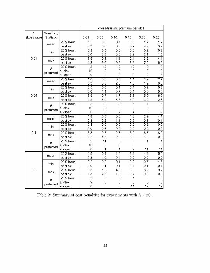
Table 2 shows this transition by summarizing the results of experiments with large call

centers - those with λ ≥ 20 - over a range of L. For each value of L and cross-training

premium p, the table summarizes the cost-penalties for the 12 different systems generated

by the parameters λ = 20, 40, 80, andM = 2, 3, 4, and 5. The column labeled ‘# preferred’

indicates the number of times out of 12 that the 80/20 heuristic, the all-flexible system, or

the all-specialist system had the lowest cost penalty. The first section of the table, with

L = 0.01, summarizes the results of Table 1 (excluding those centers with λ = 10): on

average, the 80/20 rule delivers a total cost 1% above the optimal solution.1See http://www.poms.ucl.ac.be:8080/CCServlet/servlet/home

16

In the table, we see that with L = 0.05 the 80/20 heuristic does not perform well for

the most extreme values of p, and for L = 0.1 and 0.2, the all-specialist solution is nearly

optimal except for the very lowest values of p. The square-root staffing rule reviewed in

Whitt (1992) helps to explain the superior performance of the all-specialist solution for large

L. Given an arrival load λ and a target grade of service γ, a variety of approximations

and numerical tests have shown that the level of staffing is roughly s(λ) = λ + γ√λ. The

proportional reduction in staffing achieved by crosstraining servers to handle M separate

arrival streams is,Ms(λ)− s(Mλ)

Ms(λ)=

γ¡1−M1/2

¢γ + λ1/2

. (7)

This proportion is increasing in the service grade γ and decreasing in the offered load λ.

Therefore, a very large call-center with a weak service constraint does not achieve significant

economies of scale and a significant reduction in the total number of servers by pooling cus-

tomer streams via cross-training. This implies that for our large call-centers with high values

of L, the all-specialized system is preferred for all but the lowest cross-training premiums,

and that there is a very narrow range of p in which the 80/20 heuristic is effective.

What accounts for the good performance of the 80/20 rule when L is low? Expressing

the amount of cross-training in terms of the budget, rather than in terms of the number of

servers, implicitly adjusts the solution as the cost of cross-training rises. In addition, a small

number of cross-trained servers provides most of the pooling benefits of flexibility. Therefore,

when the cross-training premium is low and the true optimal solution is to minimize the total

number of servers by having a large number of flexible servers, a small proportion of flexible

servers is sufficient to be close to the optimum.

More formally, suppose that bn > 0 and bnf > 0 are optimal interior solutions to opti-

mization problem (6). If Ψ(n, nf) is differentiable and convex in (n, nf), then the Karush-

Kuhn-Tucker (KKT) conditions are necessary and sufficient for the optimum. While it is

well-known that Erlang’s loss function is strictly convex (Messerli, 1972), the loss rate from

our network may not be convex in the number of servers for certain extreme parameters.

17

5 10 15 20 25

25

30

35

40

45

50

55

Number of Flexible Servers

Tota

l Num

ber o

f Spe

cial

ists

trade-off curve with L=-.01

optimal when p=0.25

optimal when p=0.05 tangent linewith slope -1.05

tangent linewith slope -1.25

Figure 6: Trade-off curve with L = 0.01, M = 2, and λ = 20

However, our numerical experiments indicate that the loss function is strictly convex for all

the systems considered here, and therefore the KKT conditions imply that,

−∂Ψ/∂nf |(bn,bnf )∂Ψ/∂n|(bn,bnf ) = −

(1 + (M − 1)p)M

. (8)

Define the trade-off curve n = g(nf) ≡ Ψ−1(L|nf), that is, g(nf) is the value of n, given nf ,such that Ψ(n, nf) = L. By the implicit function theorem, the left-hand side of expression

(8) is also the slope of g(nf). For low values of L, this trade-off curve has a sharp bend,

or ‘kink,’ when nf is small, so that a small range of (n, nf) satisfies expression (8) over a

wide range of M and p. However, as L rises, g(nf) becomes almost linear, and the optimal

solution moves quickly from one extreme to the other. As an example, Figure 6 shows the

total number of specialists, Mn = Mg(nf) as a function of nf for M = 2, L = 0.01 and

λ = 20. For p = 0.05 and 0.25, the figure shows the optimal solutions and the tangent lines

− (1 + (M − 1)p). Over this range of cost premiums, the optimal solution remains within

a relatively small range. In addition, if p were to rise above 0.25, the rate of change in the

18

solution will continue to decline because the trade-off curve rises even more quickly as one

moves to the left.

Finally, it is reasonable to ask whether these results are an artifact of the approximation.

To ensure that our results are accurate, we replicated a subset of the results in Tables 1 and

2 by solving numerically the balance equations of the Markov matrix for a system with two

types of customer (M = 2), and then used these ‘true’ performance measures to find the

optimal staffing configuration, the best extreme solution, and a solution guided by the 80/20

heuristic. Because of the integrality requirements, we implemented the 80/20 rule in the

actual system by choosing the configuration with spending on cross-trained servers as close

as possible to 20% of the budget (we usually found a system with flexible spending between

18% and 22%).

For the smallest systems, the difference between the results from the actual and approx-

imate systems can be large. In the most extreme example with λ = 10, L = 0.01, and

p = 0.01, the cost penalty for the 80/20 rule was 2% when using the approximation to cal-

culate the loss rate (see Table 1), but was 6.3% in the real system. This difference was due

to a combination of the integrality requirement and approximation inaccuracy. However,

significant differences disappear as the system size grows. For λ = 40 or 80, the cost penalty

incurred by the 80/20 rule for the actual system never differs from the results reported in

Tables 1 and 2 by more than 0.5%, and the average absolute difference is just 0.2%. In

addition, the additional experiments mentioned at the end of Section 5 demonstrated that

the approximation’s accuracy rises as M increases from 2 to 5. Therefore, we are confident

that for large systems our assessment of the 80/20 rule is correct.

7 Variations in the Formulation and Parameters

In the previous section we focused on the cost minimization problem, given a symmetric loss

system in which specialized and flexible servers both have equal capacity. In this section

we relax each of these assumptions. First, we consider an alternative formulation of the

19

problem: minimizing the loss probability, given a constraint on the labor budget. We also

consider systems in which flexible servers are slower than specialists and systems in which

arrival and service rates are unbalanced. We end the section by considering systems with

queueing.

7.1 Minimizing the Loss Probability with a Budget Constraint

Consider the following alternative formulation to the staffing problem:

minn,nf

Ψ(n, nf) (9)

s.t. Mn+ (1 + (M − 1)p)nf ≤ Cn ≥ 0, nf ≥ 0

where C is a budget constraint. For an interior solution to this problem, a KKT condition

is, again, (8). Therefore, it should not be surprising that the 80/20 rule works well when

solving this problem, as long as the budget C is large enough to ensure that the system has

a low loss probability.

Given this formulation, the 80/20 rule is particularly helpful for rough-cut staff planning.

Suppose that a manager knows the budget C, the cost of a specialist (say, w), and the cost

of a flexible server, wf ≡ (1 + (M − 1)p)w. The rule suggests that the manager should

deploy bn ≈ (0.8C)/(wM) specialists of each customer type as well as bnf ≈ 0.2C/wf flexibleservers. To make this staffing decision, the manager need not use a queueing model, unless

she also wishes to predict the actual system performance, given the budget.

7.2 Slower Cross-Trained Servers

Suppose that µi = µj = µ, µfi = µ

fj = µ

f , and µ > µf . We find that the 80/20 heuristic can

be extended by weighting the cost of each server by its service rate. For example, if the actual

20

1

0.8

0.6

0.4

0.2

0.05 0.1 0.15 0.2 0.25Cross-training premium (p)

Opt

imal

fract

ion

ofad

just

edbu

dget

spen

ton

cros

s-tra

ined

serv

ers Flexible servers identical to specialized

Flexible servers 10% slower than specialized

Flexible servers 20% slower than specialized

Flexible servers 30% slower than specialized

Figure 7: Optimal fraction of adjusted budget for cross-training, given slower flexible servers

(with parameters L = 0.01, M = 2, and λ = 20)

cost of a specialist is w and the actual cost of a flexible server is wf , then we can implement

an 80/20 rule using the adjusted cost per server, w = w/µ and wf = wf/µf . This extended

80/20 rule suggests that n and nf should be chosen so that wfnf/£wMn+ wfnf

¤= 0.2.

Figure 7 displays the value of this ratio for the true optimal solution with L = 0.01,M = 2

and λ = 20, and over a wide range of values for p and µ. As in Section 6, the rule is

extremely robust: results for larger M and λ are nearly identical.

7.3 Asymmetry in Service Rates and Arrival Rates

Suppose that λi 6= λj, µi 6= µj and/or µfi 6= µfj . In this case, the optimality results of Section4 may no longer hold. For example, if µfi << µ

fj , then it may at times be optimal for a

flexible server to accept a job of type i and reject a job of type j. To maintain our focus on

the optimal staffing problem, we assume that our call center maintains the routing scheme

proposed in the last section: jobs are offered to specialists, then to flexible servers, and are

never rejected if a server is available.

Given this routing policy, it is clear that the 80/20 rule is not appropriate for extreme

21

0.2

0.15

0.1

0.05

5 10 15 20

Loss prob. = 0.01

Loss prob. = 0.05

Loss prob. = 0.1

Loss prob. = 0.2O

ptim

alfra

ctio

nof

budg

etsp

ento

ncr

oss-

train

edse

rver

s

Ratio of arrival rates between type 1 and type 2 calls

Figure 8: Optimal fraction of budget for cross-trained servers, given imbalanced arrival rates

(λ1 + λ2 = 60 and p = 0.1)

cases. For example, if there are just two products, and if the load from product 1 is equivalent

to just 1 server while the load from product 2 is equivalent to 100 servers, then almost all

servers should be type-2 specialists. In this case, one also finds that the optimal system

follows an ‘N’ configuration (Garnett and Mandelbaum, 2001) with type-2 specialists, a few

cross-trained servers, and no type-1 specialists.

However, we have found that if the asymmetry is not one of these extremes, the 80/20

rule continues to work well. Figure 8 displays the optimal fraction of the budget spent on

cross-trained servers for a system with two call types over a range of values for L, the loss

probability. For all experiments we set the cross-training premium p = 0.1, µ1 = µ2 = µf = 1

and λ1 + λ2 = 60. We vary λ1/λ2, and this ratio is displayed on the horizontal axis of the

figure. For each value of λ1/λ2 and L, we found the cost-minimizing mix of dedicated and

flexible servers that met the loss probability constraint for both call types (i.e., we did not use

an aggregate loss rate, but instead provided the promised level of service to both customer

types). Our experiments suggest that while there is a slight decrease in the proportion of the

22

budget to be allocated to cross-trained server when the asymmetry increases, this decrease

is rather small (again this is especially true for small loss probabilities).

7.4 Systems with Queueing

As we mentioned in the introduction, our focus on a loss system applies directly to systems

in which significant queues rarely form either because the call center has sufficient staff

to consistently answer the call ‘on the first ring,’ or because the customers are impatient

and renege quickly. Tabordon (2002) shows that if queues are allowed to build but if the

customers’ average renege times are short (e.g., the same distribution as the service time),

then the rate of reneging is proportional to the loss probability in a system with no queues.

In this case, the 80/20 rule will again perform well if there is a tight constraint on the

reneging rate.

Now consider the other extreme: customers are infinitely patient (no reneging). We

assume that the firm’s goal is to minimize staffing costs, given a constraint on the average

waiting time - the ‘service criterion.’ To keep our focus on staffing questions, we assume

that the call center again uses simple routing and server assignment rules. Specifically,

arriving customers are first assigned to available specialists, and then to available flexible

servers (no customers are rejected). When a dedicated server becomes available, that server

is assigned a customer of its own type; when a flexible server becomes available, it is assigned

a customer from the longest queue. A similar system has been studied by Chakravarthy

and Agnihothri (2003).

To examine the performance of our heuristic for this queueing system, we first constructed

a discrete event simulation to generate performance statistics for a given staffing configura-

tion. To determine the length of each simulation run, we used a sequential procedure based

on the method of batch means (Law, 1983 pg. 998). Run lengths were sufficient to generate

a 95% confidence interval with a relative precision of 7.5%. Given that we could estimate

the performance of a particular server configuration, we used a simple search procedure to

23

find the optimal configuration, given a cross-training premium.

Using this optimization procedure, we conducted a series of tests similar to the experi-

ments that generated Tables 1 and 2, with two differences: (i) the service criterion was the

overall average wait in queue (1, 10, 30 and 60 seconds) rather than a loss probability and

(ii) because of the long run-times of the simulation we experimented with a small number of

moderately-sized systems. For each service criterion and cost-premium, we found the op-

timal configuration, 80/20 configuration, and best extreme configuration for 5 systems with

parameters M = 2, λ = 20, 40, 60, and M = 3, λ = 20, 40. Table 3 in Appendix B contains

a summary of these experiments. As in Table 2, the ‘# preferred’ indicates the number of

times out of 5 that the 80/20 heuristic, the all-flexible system, or the all-specialist system had

the lowest cost penalty. The table also shows the range of the probability of encountering a

queue, Pr{wait > 0}, for an all-flexible system in each set of five experiments. For example,when the total load Mλ = 40, Pr{wait > 0} = 0.43 for an M/M/s queue that satisfies thewaiting-time criterion of 10 sec., and when the total load Mλ = 120, Pr{wait > 0} = 0.62for the appropriate M/M/s queue.

The Table shows that the 80/20 heuristic again performs well in queueing systems with

tight service constraints, for it is always near-optimal when the service criterion is 1 sec. and

Pr{wait > 0} is around 15%. For these experiments the deviations from optimality and thecost penalties are sometimes amplified by the integrality constraint, but even so, the average

cost penalty for the 80/20 rule is usually 1% or less when the service constraint is 1 sec.

The heuristic also performs well under all service criteria when the cross-training premium

is low (p = 0.05 or below), providing more evidence that a small number of cross-trained

servers provides most of the benefits of flexibility. In fact, this phenomenon seems to be

even stronger when queueing is allowed; in this set of experiments the all-flexible system is

never preferred over the 80/20 heuristic or the all-specialist system. This preference will

not always be true (as when p = 0), but it seems that the heuristic is especially robust for

queueing systems with cross-training premiums that are relatively low. Finally, as we saw

24

in Section 6, when the service criterion is relaxed and the cross-training premium is high,

then the all-specialist system dominates. Here, this is true when the service criterion is

increased to 30 sec. or more, and the cross-training premium is higher than 0.1.

8 Summary and Additional Extensions

We have specified the optimal routing rule and proposed a simple, but effective, staffing

heuristic for large loss systems that employ both specialists and fully cross-trained severs.

This rule of thumb can be useful for managers making long-term, aggregate staffing decisions

and training decisions and can also be used as a starting point for more fine-tuning using

detailed queueing models.

Our model assumes that all service times are exponentially distributed. However, Er-

lang’s Loss function is exact with non-exponential service times, and, in general, Hayward’s

approximation works well too. Simulations performed in Tabordon (2002) demonstrate that

the performance of the approximation is not sensitive to the exponential assumption, but

we do not yet know whether the 80/20 rule continues to perform well with general service

times. We also suspect that a specialist-first routing scheme is optimal under more gen-

eral conditions, and we intend to investigate whether the optimality of the scheme holds for

systems with queues and for non-Markovian systems.

We also assume that all servers are either one-skill specialists or are trained in all skills.

In some facilities, customer service representatives may acquire multiple skills one-at-a-time,

over a long period of time. Therefore some servers may only have a subset of skills. Iravani

and Krishnamurthy (2002) consider this problem, and perform numerical experiments using

a variety of routing schemes. Some of their proposed rules, such as the “Least Skilled

Repairman” rule, are generalizations of the specialist-first rule proposed here. However,

Iravani and Krishnamurthy focus on the machine-repair problem and do not consider the

staffing problem. Finding optimal routing and staffing strategies for call centers with more

general cross-training configurations is an important and fruitful area for additional research.

25

In this article we have focused on simple, aggregate performance measures: the overall

system loss rate or average wait in queue, and the budget for labor. Given that the system

serves more than one customer type, there are a variety of alternative performance measures

to consider. If customers differ in their revenue potential, then the firm may maximize some

measure of overall profit and may offer differential service among customer types by using a

priority scheme (see Örmeci, 2002, for an analysis of revenue-based admission decisions in a

loss system) . The firm may also be concerned with balancing the workload among servers.

The specialist-first routing scheme tends to raise the utilization of specialists over the uti-

lization of the generalists, and, as suggested in Iravani and Krishnamurthy (2002), it may

be interesting to examine the trade-off between workload balancing and system efficiency.

Finally, adapting existing light-traffic approximations for queues to systems with a mix of

flexible and specialized servers may allow us to characterize the optimal mix for high-quality

systems, and perhaps generate an analytical justification for the 80/20 rule.

App e ndi x A: Opt i mal Rout i ng

The o rem 1 If µfi ≤ µi, i = 1...M , then it is optimal to route an arriving customer to a

specialist if one is available.

Proof: To characterize the optimal routing policy, we formulate the problem as an undis-

counted Markov decision process and use value iteration. Let xi be the number of occupied

specialized type i servers, let xfi be the number of type i customers in service with a flexible

server, and let xf =PM

i=1 xfi be the total number of busy flexible servers. Therefore, xi and

xfi are integers, 0 ≤ xi ≤ ni, 0 ≤ xf ≤ nf , and the vector x = (x1,..., xM,xf1 , ..., xfM) describesthe state of the system. Let v(x) be a real-valued function defined on x. Define the operator

Tiv(x) as the optimal value, given an arrival of type i and the subsequent optimal routing

of that arrival to a server (the notation used here is similar to the notation developed in de

Véricourt and Zhou, 2003).

26

Let bµf = max{µf1 , ..., µfM}. Without loss of generality, we normalize the arrival andservice rates so that

PMi=1 λi +

PMi=1 niµi + n

fbµf = 1. Let ek be a vector of zeros with a ‘1’in the position of xk, and let e

fk be a vector of zeros with a ‘1’ in the in the position of x

fk .

The dynamic operator for x is,

Γv (x) =MXi=1

λiTiv(x) +MXi=1

xiµi [1 + v (x− ei)] +MXi=1

xfi µfi

h1 + v

³x− efi

´i+

MXi=1

(ni − xi)µiv(x) +"nfbµf − MX

i=1

xfi µfi

#v(x).

The first term represents the value of an arrival. The second and third terms represent

service completions, and include a reward of ‘1’ for the throughput of a single customer.

The last two terms are due to uniformization and represent fictitious transitions from x to

itself.

Now define,

∆iv(x) = v(x+ ei)− v(x),∆fi v(x) = v(x+ efi )− v(x),

∆ifv(x) = v(x+ ei)− v(x+ efi ).

The optimal policy will follow directly from the following properties:

P.1 0 ≤ ∆iv(x), for xi < ni;

P.2 ∆fi v(x) ≤ 1, for xf < nf ;

P.3 0 ≤ ∆ifv(x), for xi < ni, xf < nf .

Property P.1 indicates that the optimal expected value is nondecreasing when a customer

is sent to an available specialist, and P.2 places an upper bound of ‘1’ on the value of sending

27

a customer to a flexible server. Property P.3 indicates that the value of routing a customer

to an available specialized server is greater than the value of routing that customer to an

available flexible server. Therefore, if v(x) satisfies properties P.1 and P.3, then it is optimal

to send an arriving customer to a specialist if one is available. Given this routing scheme,

the optimal value after a new arrival is

Tiv(x) =

v(x+ ei) if xi < ni

maxhv(x), v(x+ efi )

iif xi = ni, xf < nf

v(x) otherwise.

Note that if a specialist is not available then we may or may not send a customer to a flexible

server.

Let V be the set of all real-value functions defined on N2M that satisfy P.1, P.2 and P.3.

We will show that if v ∈ V then Γv ∈ V , and therefore, by value iteration, Tiv is the optimalvalue and ‘specialist-first’ is the optimal routing. First, it is straightforward but tedious to

show that if v ∈ V then the operator Tiv ∈ V (see Lemma 1, below).

To show that Γv satisfies P.1, we find the difference,

∆kΓv(x) = Γv(x+ ek)− Γv(x)

= µk +MXi=1

λi∆kTiv(x) +MXi=1

xiµi∆kv(x− ei) +MXi=1

xfi µfi∆kv(x− efi )

+

"(nk − xk − 1)µk +

MXi6=k(ni − xi)µi

#∆kv(x)

+

"nfbµf − MX

i=1

xfi µfi

#∆kv(x).

Because both v and Tiv satisfy P.1, ∆kΓv(x) ≥ 0.

To demonstrate that Γv satisfies P.2,

28

∆fkΓv(x) = Γv(x+ efk)− Γv(x)

= µfk +MXi=1

λi∆fkTiv(x) +

MXi=1

xiµi∆fkv(x− ei) +

MXi=1

xfi µfi∆

fkv(x− efi )

+MXi=1

(ni − xi)µi∆fkv(x) (10)

+

"nfbµf − MX

i=1

xfi µfi − µfk

#∆fkv(x).

By P.2 and the normalization assumption, ∆fkΓv(x) ≤

PMi=1 λi +

PMi=1 niµi + n

fbµf = 1.Finally, to see that Γv satisfies P.3, consider the difference,

∆kfΓv(x) =Γv(x+ ek)− Γv(x+ efk)

=MXi=1

λi∆kfTiv(x) +MXi=1

xiµi∆kfv(x− ei) +MXi=1

xfi µfi∆kfv(x− efi )

+

"(nk − xk − 1)µk +

MXi6=k(ni − xi)µi

#∆kfv(x)

+

"nfbµf − MX

i=1

xfi µfi

#∆kfv(x)

+h1−∆f

kv(x)i ³µk − µfk

´.

By using P.3, we see that all but the last term of ∆kfΓv(x) are ≥ 0. By P.2 and theassumption that µk ≥ µfk , the last term is ≥ 0. Therefore, ∆kfΓv(x) ≥ 0, Γv ∈ V , and‘specialist-first’ is the optimal routing policy. ¥

Co ro l l a r y 1 If µfi = µf , µf ≤ µi, i = 1...M , and no specialist is available, then it is optimal

to route an arriving customer to a flexible server if one is available.

Now there is no need to keep track of the ‘types’ of the customers who are in-process with

the flexible servers, and we could define a new state vector x = (x1,..., xM,xf). However, for

convenience, we will maintain the notation defined above.

29

First, define the new property,

P.20 0 ≤ ∆fi v(x) ≤ 1, for xf < nf .

If v(x) satisfies P.20 then the optimal value after a new arrival is,

T0i v(x) =

v(x+ ei) if xi < ni

v(x+ efi ) if xi = ni, xf < nf

v(x) otherwise.

so that a customer is sent to a flexible server when a specialist is not available. Let V 0 be

the set of all real-value functions defined on N2M that satisfy P.1, P.20 and P.3. Lemma

1 can be adapted to show that if v ∈ V 0 then T 0i v satisfies P.1 and P.3. Lemma 2, below,

shows that if v ∈ V 0 then T 0i v satisfies P.2

0, and therefore T0i v ∈ V 0.

From property P.20 and equation 10 above, 0 ≤ ∆fkΓv(x) ≤ 1, so that Γv satisfies

P.20. The remainder of the proof of Theorem 1 demonstrates that Γv satisfies P.1 and P.3.

Therefore, a specialist-then-flexible routing scheme is optimal.

Lemma 1 If v ∈ V , then Tiv ∈ V.

P.1: To show that 0 ≤ ∆kTiv(x), for xk < nk, consider the following six cases.

xi < ni − 1 : ∆kTiv(x) = Tiv(x+ ek)−Tiv(x ) = v(x+ ek+ ei)− v(x+ ei) ≥ 0 by P.1.

xi = ni − 1, i = k, xf < nf ∆kTkv(x) = maxhv(x+ ek), v(x+ ek + e

fk)i− v(x+ ek) ≥

0.

xi = ni − 1, i = k, xf = nf ∆kTkv(x) = v(x+ ek)− v(x+ ek) = 0.

xi = ni − 1, i 6= k : ∆kTiv(x) = v(x+ ek + ei)− v(x+ ei) ≥ 0 by P.1.

xi = ni, xf < nf : ∆kTiv(x) =

maxhv(x+ ek), v(x+ ek + e

fi )i−max

hv(x), v(x+ efi )

i≥ 0 by P.1.

xi = ni, xf = nf : ∆kTiv(x) = v(x+ ek)− v(x) ≥ 0 by P.1.

30

P.2: To show that ∆fkTiv(x) ≤ 1, for xf < nf , consider three cases.

xi < ni : ∆fkTiv(x) = Tiv(x+ e

fk)− Tiv(x) = v(x+ efk + ei)− v(x+ ei) ≤ 1 by P.2.

xi = ni, xf < nf − 1 : ∆f

kTiv(x) = maxhv(x+ efk), v(x+ e

fk + e

fi )i−max

hv(x), v(x+ efi )

i≤

1 by P.2.

xi = ni, xf = nf − 1 : ∆f

kTiv(x) = v(x + efk) − maxhv(x), v(x+ efi )

i≤ v(x + efk) −

v(x) ≤ 1 by P.2

P.3: To show that ∆kfTiv(x) ≥ 0, for xk < nk,and xf < nf , consider five cases.

xi < ni − 1 : ∆kfTiv(x) = Tiv(x+ek)−Tiv(x+efk) = v(x+ek+ei)−v(x+efk+ei) ≥ 0by P.3.

xi = ni − 1, i 6= k : ∆kfTiv(x) = v(x+ ek + ei)− v(x+ efk + ei) ≥ 0 by P.3.xi = ni − 1, i = k : ∆kfTkv(x) = max

hv(x+ ek), v(x+ ek + e

fk)i− v(x+ efk + ek) ≥ 0.

xi = ni, xf < nf − 1 : ∆kfTiv(x) = max

hv(x+ ek), v(x+ ek + e

fi )i−max

hv(x+ efk), v(x+ e

fk + e

fi )i

0 by P.3.

xi = ni, xf = nf − 1 : ∆kfTiv(x) = max

hv(x+ ek), v(x+ ek + e

fi )i−v(x+efk) ≥ v(x+

ek)− v(x+ efk) ≥ 0 by P.3. ¥

Lemma 2 If v ∈ V 0, then T 0i v satisfies P.2

0.

P.20: To show that 0 ≤ ∆fkT

0i v(x) ≤ 1, for xf < nf , consider three cases.

xi < ni : ∆fkT

0i v(x) = T

0i v(x+ e

fk)− T 0

i v(x) = v(x+ efk + ei)− v(x+ ei) ≥ 0 and ≤ 1

by P.20.

xi = ni, xf < nf − 1 : ∆f

kT0i v(x) = v(x+ e

fk + e

fi )− v(x+ efi ) ≥ 0 and ≤ 1 by P.20.

xi = ni, xf = nf − 1 : ∆f

kT0i v(x) = v(x+ e

fk)− v(x+ efi ) = 0. This last equality is due

to the assumption that µfk = µfi = µf and can itself be demonstrated by value

iteration. ¥

31

App endi x B: Tabl es

m (# call types)

λ (arrival rate per group)

utilization for all-flexible system 0.01 0.05 0.10 0.15 0.20 0.25

20% heur. 2.0 0.9 0.6 0.3 0.3 0.2 best ext. 0.1 2.2 5.5 9.1 10.6 9.6 20% heur. 1.1 0.2 0.1 0.0 0.2 0.2 best ext. 0.0 2.3 5.9 8.2 7.3 6.6 20% heur. 0.8 0.8 0.8 0.6 0.5 0.8 best ext. 0.2 3.3 6.7 5.6 4.7 4.2 20% heur. 0.3 0.1 0.3 0.6 1.0 1.4 best ext. 0.0 3.0 3.8 3.3 2.9 2.5 20% heur. 5.0 1.7 0.5 0.2 0.1 0.1 best ext. 0.1 2.7 8.7 13.0 11.1 9.6 20% heur. 2.7 0.5 0.0 0.1 0.2 0.4 best ext. 0.0 3.8 10.6 8.9 7.5 6.4 20% heur. 1.3 0.1 0.1 0.5 0.8 1.3 best ext. 0.0 4.9 6.9 5.6 4.7 3.9 20% heur. 0.5 0.4 0.3 1.1 1.7 2.3 best ext. 0.3 6.0 4.3 3.4 2.7 2.2 20% heur. 6.3 1.8 0.5 0.2 0.1 0.2 best ext. 0.1 4.1 13.0 13.0 10.8 8.9 20% heur. 3.4 0.5 0.0 0.2 0.5 0.8 best ext. 0.0 5.9 10.9 8.7 7.1 5.8 20% heur. 1.5 0.2 0.2 0.7 1.3 1.9 best ext. 0.2 8.0 7.0 5.4 4.3 3.4 20% heur. 0.6 0.3 0.8 1.6 2.4 3.2 best ext. 0.7 6.2 4.3 3.2 2.4 1.8 20% heur. 7.1 1.7 0.4 0.0 0.1 0.4 best ext. 0.1 5.9 16.1 12.6 10.1 8.2 20% heur. 3.5 0.4 0.1 0.3 0.8 1.2 best ext. 0.1 8.4 10.8 8.3 6.5 5.2 20% heur. 1.5 0.0 0.4 1.1 1.8 2.6 best ext. 0.5 9.6 6.8 5.0 3.8 2.9 20% heur. 0.5 0.2 1.1 2.1 3.2 4.1 best ext. 1.2 6.0 4.1 2.9 2.1 1.5

5

10 0.78

20 0.85

40 0.90

80 0.93

4

10 0.76

20 0.83

40 0.88

80 0.92

0.88

3

10 0.72

20 0.80

40 0.86

80 0.91

cross-training premium per skill

2

10 0.67

20 0.76

40 0.83

80

Table 1: Cost penalties as a percentage of the optimal solution, with loss rate L = 0.01

32

L(Loss rate)

SummaryStatistic 0.01 0.05 0.10 0.15 0.20 0.25

20% heur. 1.5 0.3 0.4 0.8 1.2 1.7 best ext. 0.3 5.6 6.8 5.7 4.7 3.9 20% heur. 0.3 0.0 0.0 0.0 0.2 0.2 best ext. 0.0 2.3 3.8 2.9 2.1 1.5 20% heur. 3.5 0.8 1.1 2.1 3.2 4.1 best ext. 1.2 9.6 10.9 8.9 7.5 6.6 20% heur. 2 12 12 12 10 9all-flex 10 0 0 0 0 0all-spec. 0 0 0 0 2 3 20% heur. 1.8 0.3 0.5 1.1 1.9 2.7 best ext. 0.3 3.5 2.8 1.8 1.2 0.8 20% heur. 0.5 0.0 0.1 0.1 0.2 0.3 best ext. 0.0 1.4 0.7 0.1 0.0 0.0 20% heur. 3.9 0.7 1.7 3.3 5.0 6.5 best ext. 1.2 8.0 5.3 4.0 3.2 2.6 20% heur. 2 12 10 8 4 3all-flex 10 0 0 0 0 0all-spec. 0 0 2 4 8 9 20% heur. 1.8 0.3 0.8 1.8 2.9 4.1 best ext. 0.3 2.2 1.1 0.5 0.3 0.1 20% heur. 0.4 0.0 0.0 0.2 0.2 0.5 best ext. 0.0 0.6 0.0 0.0 0.0 0.0 20% heur. 3.8 0.7 2.8 5.0 6.7 8.2 best ext. 1.2 4.8 2.9 1.9 1.2 0.8 20% heur. 2 11 8 3 1 1all-flex 10 0 0 0 0 0all-spec. 0 1 4 9 11 11 20% heur. 1.5 0.4 1.6 3.1 4.4 5.6 best ext. 0.3 1.0 0.4 0.2 0.2 0.2 20% heur. 0.2 0.0 0.1 0.3 0.7 1.6 best ext. 0.0 0.1 0.1 0.1 0.1 0.1 20% heur. 3.3 1.6 4.3 6.5 8.2 9.7 best ext. 1.3 2.6 1.3 0.7 0.3 0.3 20% heur. 3 8 3 1 0 0all-flex 9 0 0 0 0 0all-spec. 0 3 8 11 12 12

cross-training premium per skill

mean

min

0.1

mean

min

max

#preferred

max

#preferred

0.01

0.05

mean

min

max

#preferred

0.2

mean

min

max

#preferred

Table 2: Summary of cost penalties for experiments with λ ≥ 20.

33

service criterion (sec.)

range for Pr{wait>0}

SummaryStatistic 0.01 0.05 0.10 0.15 0.20 0.25

20% heur. 1.2 1.1 0.7 0.6 0.6 0.8 best ext. 1.0 4.8 5.8 4.6 3.7 3.0 20% heur. 0.4 0.1 0.2 0.4 0.3 0.0 best ext. 0.7 3.5 3.6 2.9 2.3 1.8 20% heur. 2.3 1.9 1.1 0.8 0.8 1.4 best ext. 1.4 7.0 8.3 6.3 4.9 3.8 20% heur. 2 5 5 5 5 5all-flex 3 0 0 0 0 0all-spec. 0 0 0 0 0 0 20% heur. 0.9 0.7 1.0 1.5 2.1 2.5 best ext. 1.4 3.3 2.5 1.9 1.5 1.2 20% heur. 0.1 0.2 0.5 0.8 1.2 1.7 best ext. 0.7 1.3 1.0 0.8 0.5 0.4 20% heur. 1.6 1.2 1.6 2.3 3.1 3.9 best ext. 2.4 5.5 3.6 3.1 2.7 2.2 20% heur. 5 5 4 3 3 1all-flex 0 0 0 0 0 0all-spec. 0 0 1 2 2 4 20% heur. 0.1 0.7 1.4 2.1 2.5 3.2 best ext. 1.3 2.6 2.1 1.7 1.4 1.1 20% heur. 0.1 0.5 0.9 1.7 1.9 2.3 best ext. 0.9 1.4 1.1 0.9 0.6 0.4 20% heur. 0.2 0.9 2.1 3.3 4.0 4.8 best ext. 1.8 4.4 4.0 3.7 3.3 2.9 20% heur. 5 5 4 2 1 1all-flex 0 0 0 0 0 0all-spec. 0 0 1 3 4 4 20% heur. 0.3 1.1 1.7 2.1 2.9 3.5 best ext. 1.1 1.2 0.7 0.4 0.2 0.0 20% heur. 0.1 0.5 1.0 1.1 1.4 1.8 best ext. 0.8 0.6 0.3 0.1 0.0 0.0 20% heur. 1.0 1.9 2.9 3.6 4.4 5.3 best ext. 1.7 1.9 1.4 1.0 0.5 0.0 20% heur. 5 2 1 0 0 0all-flex 0 0 0 0 0 0all-spec. 0 3 4 5 5 5

cross-training premium per skill

1

mean

min

max

#preferred

0.12 - 0.17

10

mean

min

max

#preferred

0.43-0.62

30

mean

min

max

#preferred

0.67 - 0.79

60

mean

min

max

#preferred

0.82 - 0.89

Table 3: Summary of cost penalties from the queueing simulation.

Acknowl e dgements

We are grateful to Chris Wright for creating the queueing simulation described in section

7.4. We would also like to thank Paul Schweitzer for his helpful comments.

34

Ref erences

Agnihothri, S. R. (2003), “Server Flexibility in a Queueing System with Heterogeneous

Customers,” working paper, School of Management at Binghamton University, State

University of New York.

Agnihothri, S. R., A. K. Mishra, and D. E. Simmons (2003), “Workforce cross-training

decisions in field service,” forthcoming in the Journal of the Operational Research

Society.

Aksin, O. Z. and F. Karaesmen (2002), “Designing Flexibility: Characterizing the Value of

Cross-Training Practices,” INSEAD working paper,

http://home.ku.edu.tr/~fkaraesmen/pdfs/flex2102.pdf.

Armony, M. and C. Maglaras (2001), “On customer contact centers with a call-back option:

customer decisions, routing rules, and system design,” forthcoming in Operations Re-

search,

http://www-1.gsb.columbia.edu/faculty/cmaglaras/papers/static.pdf.

Armony, M. and C. Maglaras (2002), “Contact centers with a call-back option and real-time

delay information,” forthcoming in Operations Research,

http://www-1.gsb.columbia.edu/faculty/cmaglaras/papers/dynamic.pdf.

Borst, S.C, A. Mandelbaum, and M.I. Reiman. (2004), “Dimensioning large call centers,”

Operations Research, vol. 52, no. 1..

Borst, S. C., P. Seri. (2000), “Robust algorithms for sharing agents with multiple skills.”

Working paper, CWI, Amsterdam, The Netherlands.

Chakravarthy, S. R. and S. R. Agnihothri (2003), “Impact of Worker Cross-training in

Service Systems with Two Types of Customers” Binghamton University working paper,

http://som.binghamton.edu/faculty/agnihothri.htm.

35

Chevalier, P. and N. Tabordon (2003), “Overflow Analysis and Cross-Trained Servers,”

International Journal of Production Economics, 85, pg. 47-60.

de Vericourt, F. and Y. Zhou, “Managing Response Time and Service Quality in a Call

Routing Problem,” working paper, Business School, University of Washington, Seattle,

http://faculty.washington.edu/yongpin/Response_Time_and_Service_Quality.pdf.

Ewalt, D. M. (2003), “Opportunity on the Line,” InformationWeek, Feb 24, 2003, Issue

928; pg. 65.

Fredericks, A. A. (1980), “Congestion in Blocking Systems - A Simple Approximation

Technique,” The Bell System Technical Journal, vol. 59, No. 6.

Gans, N., G. Koole and A. Mandelbaum (2003), “Telephone Call Centers: Tutorial, Re-

view and Research Prospects,” Manufacturing & Service Operations Management

(M&SOM), vol. 5, no. 2.

Gans, N. and G. van Ryzin (1997), “Optimal Control of a Multiclass, Flexible Queueing

System”, Operations Research, vol. 45, no. 5.

Garnett. O. and A. Mandelbaum (2001), “An introduction to skills-based routing and its

operational complexities,” Teaching note, Technion, 2001,

http://ie.technion.ac.il/serveng/Homeworks/HW9.pdf.

Garnett, O., A. Mandelbaum, and M Reiman (2002), “Designing a Call Center with Impa-

tient Customers” MSOM vol. 4 n. 3 pp.208-227.

Guerin, R. and L. Y.-C. Lien (1990), “Overflow Analysis for Finite Waiting Room Systems,”

IEEE Transactions on Communications, vol. 38, no. 9.

Green, L. (1985), “A Queuing System with General-Use and Limited-Use Servers,” Oper-

ations Research, vol. 33, no. 1.

36

Gurumurthi, S. and S. Benjaafar (2001), “Modeling and Analysis of Flexible Queueing

Systems,” forthcoming in Naval Research Logistics,

http://www.me.umn.edu/divisions/ie/logistics/flexq.pdf.

Harrison, J. M. and M. J. López (1999), “Heavy Traffic Resource Pooling in Parallel-Server

Systems,” Queueing Systems, Vol. 33, 339-368.

Harrison, J.M. and A. Zeevi (2003), “Method for Staffng Large Call Centers Based on Sto-

chastic Fluid Models,” working paper, Stanford University and Columbia University,

http://faculty-gsb.stanford.edu/harrison/personal_page/CC-staffing-revised.pdf.

Hopp, W. and M. P. van Oyen (2003), “Agile Workforce Evaluation: A Framework for

Cross-training and Coordination,” working paper, Northwestern University, IEMS,

WorkSmart Laboratory, 2003.

http://gsbdata.wt.luc.edu/~vanoyen/research/AWE-IIE-Hopp-VanOyen.pdf·

Iravani, S.M.R. and V. Krishnamurthy (2002) “Workforce Agility in Repair and Mainte-

nance Environments.” working paper, Northwestern University, IEMS.

Jagerman, D. L. (1984), “Methods in Traffic Calculations”. AT&T Bell Laboratories Tech-

nical Journal, Vol. 63, No. 7, pp. 1283-1310.

Koole, G. and J. Talim (2000), “Exponential Approximation of Multi-Skill Call Centers

Architecture,” Proceedings of QNETs 2000, 23/1-10, Ilkley (UK).

Law, A. M. (1983), “Statistical Analysis of Simulation Output Data.” Operations Resarch,

Vol. 31, No. 6, pp. 983-1029.

Messerli, E. J. (1972), “Proof of a Convexity Property of the Erlang B Formula,” Bell

Systems Technical Journal, vol. 51, pg. 951.

Mitchell, I. (2001), “Call Center Consolidation — Does It Still Make Sense?” Business

Communications Review, December, 2001, pg. 24,

http://www.bcr.com/bcrmag/2001/12/p24.asp.

37

Örmeci L. (2002), “Dynamic admission control in a call center with one shared and two

dedicated service facilities.” To appear in IEEE Transactions on Automatic Con-

trol. Currently available as EURANDOM Technical Report 2002-044, Eindhoven,

http://www.eurandom.nl/Past%20years/reports/2002/044loreport.pdf.

Ross, K. W. (1995), “Multiservice Loss Models for Broadband Telecommunication Net-

works,” Springer, Berlin.

Shumsky, R. A. (2003), “Approximation and Analysis of a Queueing System with Flexible

and Specialized Servers”, to appear in OR Spectrum,

http://omg.ssb.rochester.edu/omgHOME/shumsky/flex_serv.PDF.

Stanford, D. A. and W. K. Grassmann (1993),“The Bilingual Server System: A Queueing

Model Featuring Fully and Partially Qualified Servers.” INFOR, vol. 31, no. 4.

Stolletz, Raik. (2003) “Performance Analysis and Optimization of Inbound Call Centers,”

Lecture Notes in Economics and Mathematical Systems. Springer, Berlin.

Tabordon, N. (2002), “Modeling and Optimizing the Management of Operator Training in a

Call Center,” Ph.D. Dissertation, Institut D’Administration et de Gestion, Universite

Catholique de Louvain, Louvain-la-Neuve, Belgium.

Wallace, R.B. and W. Whitt (2004), “Resource Pooling and Staffing in Call Centers with

Skill-Based Routing,” working paper, Columbia University,

http://www.columbia.edu/~ww2040/pooling2.pdf.

Whitt, W. (1984), “Heavy-Traffic Approximations for Service Systems With Blocking,”

AT&T Bell Laboratories Technical Journal Vol 63 No 5, May-June.

Whitt, W. (1992), “Understanding the Efficiency of Multi-Server Service Systems,” Man-

agement Science, 38, pp. 708-723.

38