Rotational fatigue analysis on Shanghai 65-m fully ...

J. Astrophys. Astr. (2019) 40:30 © Indian Academy of Scienceshttps://doi.org/10.1007/s12036-019-9599-9

Rotational fatigue analysis on Shanghai 65-m fully-steerable antennastructure during its normal operation

YAN LIU

School of Civil Engineering, Chang’an University, Chang’an Middle Road, No.75, Xi’an 710061,People’s Republic of China.E-mail: [email protected]

MS received 19 February 2019; accepted 29 May 2019

Abstract. Structural fatigue property of Shanghai 65-m fully-steerable antenna structure is analysed. Accord-ing to the active fully-steerable working pattern, the typical fatigue stress piece is put forward based on simplesampling and decomposed by real-time rain flow counting algorithms. Subsequently, the fatigue lives of pitchmechanism bearings were computed by miner linear accumulative damage criterion. What’s more, in a completecycle of dynamic observation, the shear force and axial force of high strength friction grip bolts for all of thesupporting nodes are extracted and counted aiming at each pitching angle. As a result, fatigue analysis is carriedout on the supporting nodes of the back-frame structure connected with the pitching mechanism. Last but notthe least, finite element refinement model is conducted for the contact part between antenna wheels and the rail.Based on contact fatigue curve spectrum, the contact fatigue existing between the antenna structure roller andthe track is analysed. The results show that the fatigue life of the whole antenna structure can meet the safetyrequirements in the design reference period which is intended to be 30 years. This systematic fatigue analysisprocedure, method and results can provide valuable references for design, construction and maintenance ofsuch similar fully-steerable antenna structures in future.

Keywords. Antenna structure—fatigue—simple sampling—real-time rain flow—miner.

1. Introduction

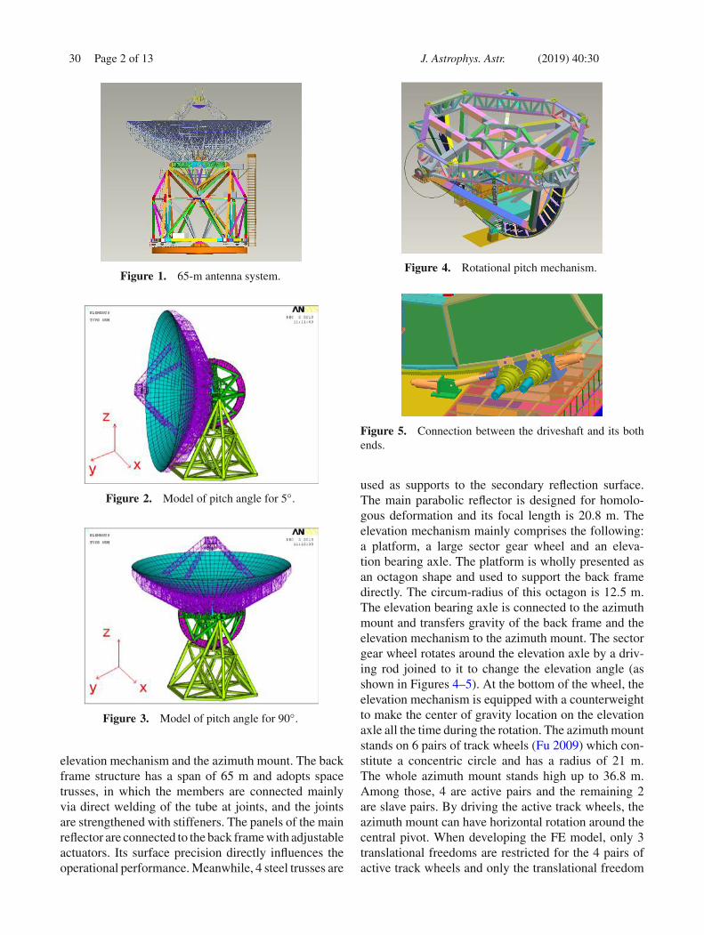
In order to carry out the mission of the lunar probe pro-gram including Chang’e-2, Chang’e-3 and various otherscientific deep-space explorations, Chinese Academy ofSciences, Shanghai Municipal Government and LunarProbe Program jointly invested in the construction ofa sixty-five-meter aperture antenna in Shanghai (seeFigure 1), China. It was completed at the end of 2012and it was the largest in Asia and the third largest in theworld, among the advanced fully-steerable antennae.During the operation, antenna structure will randomlyfulfill observations 60 times within the pitching angleof 5◦–90◦ each day (see Figures 2–3). The number ofworking days for the structure is 340 per year and thedesign reference period is 30 years (Fu 2009), i.e. theantenna structure must meet the required cycles of times(60 × 340 × 30 = 612000).

The part above the wheel structure could rotatearound the elevation axis to accomplish random obser-vation during its operation, accompanied by rotation

around the central pivot (axis Z ). Such operation mech-anism is really a special and long-term fatigue load tothe antenna structure and as a result leads to structuralfatigue problems. As fatigue failure is characterized byits brittleness and in the event of occurrence, the conse-quences could be disastrous. So it is extremely crucial toanalyse its fatigue problem and estimate if the key com-ponent will fail during the design reference period (for30 years). The analysis results could provide guidancefor the safe operation and maintenance of the structure(Wu 2016; Weng 2017; Xu & Zhan 2017; Liu 2016).However, the research on the fatigue problem caused byits rotation operation has almost never been reported athome and abroad.

2. Structural form and development of the FEmodel of the antenna

The model of Shanghai 65-m antenna structure con-sists of three main parts: the back frame structure, the

0123456789().: V,-vol

http://crossmark.crossref.org/dialog/?doi=10.1007/s12036-019-9599-9&domain=pdf

30 of 13 J. Astrophys. Astr. (2019) 40:30

Figure 1. 65-m antenna system.

Figure 2. Model of pitch angle for 5◦.

Figure 3. Model of pitch angle for 90◦.

elevation mechanism and the azimuth mount. The backframe structure has a span of 65 m and adopts spacetrusses, in which the members are connected mainlyvia direct welding of the tube at joints, and the jointsare strengthened with stiffeners. The panels of the mainreflector are connected to the back frame with adjustableactuators. Its surface precision directly influences theoperational performance. Meanwhile, 4 steel trusses are

Figure 4. Rotational pitch mechanism.

Figure 5. Connection between the driveshaft and its bothends.

used as supports to the secondary reflection surface.The main parabolic reflector is designed for homolo-gous deformation and its focal length is 20.8 m. Theelevation mechanism mainly comprises the following:a platform, a large sector gear wheel and an eleva-tion bearing axle. The platform is wholly presented asan octagon shape and used to support the back framedirectly. The circum-radius of this octagon is 12.5 m.The elevation bearing axle is connected to the azimuthmount and transfers gravity of the back frame and theelevation mechanism to the azimuth mount. The sectorgear wheel rotates around the elevation axle by a driv-ing rod joined to it to change the elevation angle (asshown in Figures 4–5). At the bottom of the wheel, theelevation mechanism is equipped with a counterweightto make the center of gravity location on the elevationaxle all the time during the rotation. The azimuth mountstands on 6 pairs of track wheels (Fu 2009) which con-stitute a concentric circle and has a radius of 21 m.The whole azimuth mount stands high up to 36.8 m.Among those, 4 are active pairs and the remaining 2are slave pairs. By driving the active track wheels, theazimuth mount can have horizontal rotation around thecentral pivot. When developing the FE model, only 3translational freedoms are restricted for the 4 pairs ofactive track wheels and only the translational freedom

J. Astrophys. Astr. (2019) 40:30 of 13 30

Table 1. Finite element from ANSYS.

Component Element

Back frame, supports of sub-reflector Pipe 16Core-tube, elevation wheel Shell 63Elevation mechanism, azimuth mount, actuator Beam 4Drive spindle of elevation Link 8Feed source, counterweight Mass 21Panels of main reflector Shell 181

Table 2. Material properties.

Properties Steel Aluminum alloy

Elastic modulus (N/m2) 2.06 × 1011 0.7 × 1011

Poisson’s ratio (λ) 0.3 0.3Density ρ (kg/m3) 7850 2700

in the Z-direction is restricted for 2 pairs of the slavetrack wheels. For the central pivot, only the transla-tional Z-direction and the rotational freedom around theZ axis are restricted. Considering the mechanical char-acteristics of different components, different elementsare employed to simulate a component using ANSYS.Specific elements and material properties used in theFE model are listed in Tables 1 and 2. The componentssuch as the feed, platform, guard rails and the gener-ator room, which are not load-carrying, are treated aslumped mass and applied to the corresponding nodes inthe FE model.

3. Pitch mechanism bearings fatigue analysis

3.1 Composition of fatigue stress spectrum

In the analysis of fatigue life of the fully-steerableantenna structure, it is necessary to analyse the fatiguestress spectrum during active shape-changing work-ing pattern. Therefore, complete observation work canbe defined initially as randomly searching (from 5◦ to90◦) and subsequently as continuously tracking until theobservation could not be tracked. The object searchingand tracking for the pitching mechanism of the antennastructure is essentially the same. Although the trackingprocess is a dynamic process, due to slow movement,the rotation velocity of the pitching mechanism is about0.3◦/s and such tracking motion process is similar tothe quasi-static process. Based on Ansys software, theparametric finite element analysis program for random

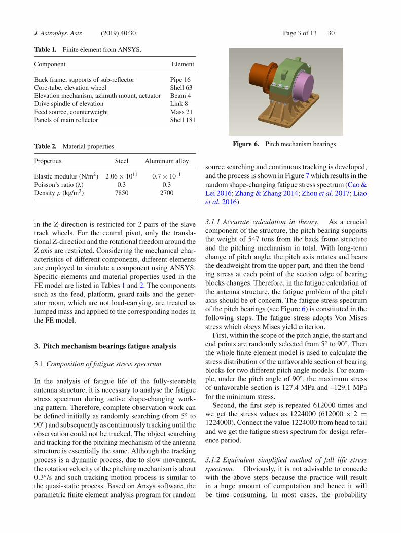
Figure 6. Pitch mechanism bearings.

source searching and continuous tracking is developed,and the process is shown in Figure 7 which results in therandom shape-changing fatigue stress spectrum (Cao &Lei 2016; Zhang & Zhang 2014; Zhou et al. 2017; Liaoet al. 2016).

3.1.1 Accurate calculation in theory. As a crucialcomponent of the structure, the pitch bearing supportsthe weight of 547 tons from the back frame structureand the pitching mechanism in total. With long-termchange of pitch angle, the pitch axis rotates and bearsthe deadweight from the upper part, and then the bend-ing stress at each point of the section edge of bearingblocks changes. Therefore, in the fatigue calculation ofthe antenna structure, the fatigue problem of the pitchaxis should be of concern. The fatigue stress spectrumof the pitch bearings (see Figure 6) is constituted in thefollowing steps. The fatigue stress adopts Von Misesstress which obeys Mises yield criterion.

First, within the scope of the pitch angle, the start andend points are randomly selected from 5◦ to 90◦. Thenthe whole finite element model is used to calculate thestress distribution of the unfavorable section of bearingblocks for two different pitch angle models. For exam-ple, under the pitch angle of 90◦, the maximum stressof unfavorable section is 127.4 MPa and –129.1 MPafor the minimum stress.

Second, the first step is repeated 612000 times andwe get the stress values as 1224000 (612000 × 2 =1224000). Connect the value 1224000 from head to tailand we get the fatigue stress spectrum for design refer-ence period.

3.1.2 Equivalent simplified method of full life stressspectrum. Obviously, it is not advisable to concedewith the above steps because the practice will resultin a huge amount of computation and hence it willbe time consuming. In most cases, the probability


Continuous shape-changing fatigue stress spectrum is

established

Randomly select the observation pitching angle βi

Structural finite element simulation corresponding to βi is

carried out

Continuous tracking process is calculated from 5° to 90° in

every 5 degrees

Continuous searching is carried out until observation could not be

tracked

Figure 7. Flow diagram of fatigue stress spectrum compu-tation.

at each pitch angle of the antenna structure is equalduring its long-term observation. Hence the fatiguedamage accumulation of the structure during eachobservation could be determined. Therefore, in a statis-tical sense, it could be considered that the total damageaccumulation caused by the stress time history of a cer-tain number of observations is approximately the sameas the result of 6,12,000 times, i.e.

num =(

λM

E

)2

,

where λ is the reliability index. For a large sample,the bilateral quantile corresponding with the guaranteedrate α is adopted. For a small sample, the bilateral quan-tile corresponding to t distribution function is adopted.Usually when individual number is more than 30, thesample could be considered as a large sample and onthe contrary, it is a small sample. Also, M is the totalvariation coefficient and adopts 0.5775 according to theuniform distribution function within the scope [0, 1],and E is the fractional error between the sampling meanand the ensemble mean.

Take the guaranteed rate α = 99% (query standard-ized normal distribution function λ = 2.5775). Therelative error of the sampling mean value does notexceed 5%, and hence at least 885 samples need tobe taken. In this research, 1000 samples were taken,namely 1000 models were randomly taken from 5◦to 90◦, then the stress distributions of the unfavorablesection were calculated and a standard fatigue stressspectrum (shown in Figure 8) was formed. Finally, thecomposition process of the standard fatigue stress spec-trum was repeated a number of times until the fatiguechecking results became stable (Zhou et al. 2015)

Figure 8. A standard fatigue stress spectrum.

3.2 Miner linear cumulative damage criterion

The Miner linear cumulative damage criterion (seeEquation (1)) is usually used to deal with variableamplitude fatigue problems. The criterion is to assumethat the equal amplitude fatigue life of each stresslevel is Ni , the actual cycle number is ni and theresulting energy is wi under the variable amplitudestress �σ , �σ2, . . . , �σk. The structure will rupturebecause of the shift in fatigue when all the energy accu-mulates to W , where W refers to the critical value of thetotal energy absorbed by the material during the stresscycle∑ wi

W=

∑ niNi

= 1. (1)

The success of the criterion lies in the huge numberof test results (especially for random fatigue load test)which show that the average of the algebraic expression∑

(ni/Ni) is close to 1. This concept is clear and the for-mula is concise and hence this criterion has an extensiveapplication in engineering (Zhao et al. 2016; Li et al.2018). Other methods require extensive experiments tofit many parameters and the result accuracy is not betterthan Miner criterion.

This fully-steerable antenna structure could operateat any pitch angle, so the load from its mechanical trans-mission part is obviously a random variable amplitudefatigue load. As for the variable amplitude fatigue prob-lem, if stress levels at all levels and the correspondingfrequency could be estimated, variable stress amplitudewill be converted to an equivalent constant stress ampli-tude. Then fatigue analysis of the pitch bearing will becarried out according to the process shown in Figure 9.

3.3 Decomposition of fatigue stress spectrum byrain-flow counting in real time

Currently the mostly used fatigue stress spectrumdecomposition method is the rain-flow counting


Establsih fatigue stress spectrum by randomly sampling within the domain of pith angles

Acquire average constant stress amplitude and corresponding frequency of occurrence by rain flow

counting method

Determine life Ni at each constant stress level according to the relationship between stress and

cycle life

Analyse the structure fatigue problem based on the Miner linear cumulative damage criterion

Figure 9. Analysis flowchart.

method. Taking the longitudinal coordinate straightdown as time and the horizontal coordinate as stress,the stress-time history is similar to the rain flow streamdown from the vertex. This method is a counting methodwhich has considered stress–strain relationship of thematerial (Liu et al. 2017a). Namely, in application, aseries of closed stress–strain hysteretic curves are putforward from sample records by such a method, andthus the corresponding mean value and the amplitudeof each stress cycle are proposed.

In this paper, a new real-time rain flow countingmethod (Fan & Jin 2010) is adopted, and the corre-sponding program is developed. The real-time countingmodel of the rain flow overcomes the limitation ofreconstructing the load-time history before counting inthe traditional method, and it does not need to re-adjustor dock the load-time history. It is not only suitable forall kinds of existing data processing, but also appliedto the dynamic real-time data processing. For fullysteerable antenna structure, this method can be usedto calculate and analyse the fatigue damage in real timeafter several times of shape-changing during the oper-ation and thus to fatigue life estimation. When Minerlinear cumulative damage criterion is applied, the count-ing method needs to be adopted in order to calculate thecycling frequency of stress amplitude at all levels (Wang& Gu 2008; Fu et al. 2016; Liu et al. 2017b).

When rain flow counting method is applied, firstly,the peak-to-valley values are extracted in the actualstrain-time history curve. Secondly, the extracted peak-to-valley data record is rotated to 90 degrees. As shownin Figure 10, the time axis is vertically down, the datarecords are like a series of roofing, and the ‘rain’ goesdown the roof. The stress cycle is determined from the

Figure 10. Rain flow counting diagram.

rain-flow trace so that this process is vividly called asthe rain-flow counting method. This method has consid-ered the stress–strain behaviors of the material. A seriesof closed stress–strain hysteresis loops are determinedby the rain flow method according to sample recordsand thus the mean and amplitude of the correspondingstress cycle is obtained.

According to the rain flow counting principle men-tioned above, based on MATLAB, the correspond-ing program is programmed. For the standard stressspectrums obtained, they are decomposed by the rain-flow counting program and the results are shown inFigure 10.

3.4 Fatigue life of different levels of stress

According to the steel structure design code in China(GB50017-2017), the fatigue life corresponding to eachdecomposed stress cycle could be determined by theparameters characterized by the metal body as

[�σ ] =(C

n

)1/β

, (2)

where C = 1940 × 1012, β = 4, n is stress cycle timesand [�σ ] is the allowable stress amplitude (Figure 11).

In view of antenna operation characteristics, its obser-vation times could be used to express fatigue life.Specifically, we use the standard stress spectrum in the


Figure 11. Decomposition result by using rain flow count-ing method.

calculation of fatigue life. The Miner linear cumulativedamage criterion could be equivalently expressed inEquation (3). It shows a standard stress spectrum cyclesT times and then the structure fails. In order to calcu-late it in a simplified manner, a uniform and set stresshistory can be adopted to repeat and substitute the longterm of the actual stress cycle on the structure. So thisuniform and set stress history can be defined as the stan-dard stress spectrum:

T

(k∑

i=1

niNi

)= 1, (3)

where T is the number of stress-history spectrum at thetime of failure, k is the total number of different levelsof the stress decomposed from a standard stress historyspectrum, ni is the cycle of a certain level of stress ina standard stress-history spectrum, Ni is the constantamplitude fatigue life of a certain level of stress in astandard stress history spectrum. Hence the fatigue lifeN could be calculated as follows:

N = num(k∑

i=1

niNi

) . (4)

Since the standard stress spectrum is not uniquelydetermined, it is necessary to construct the stochasticsimulations of the standard stress spectrum a numberof times. The number of simulation calculations shouldsatisfy Equations (5) and (6), i.e. after these simulations,the mean and the standard deviation of the structuralfatigue life tend to be stable.∣∣NT ( j) − NT ( j − check)

∣∣NT ( j)

≤ 0.1%, (5)∣∣σNT ( j) − σNT ( j − check)

∣∣σNT ( j)

≤ 0.1%, (6)

where NT ( j) is the average fatigue life of the struc-ture after simulations and σNT ( j) is the deviation of thestructural fatigue life after simulations.

Figure 12. Average fatigue life of pitch axis after manysimulations.

Figure 13. Standard deviation of fatigue life after manysimulations.

Figure 14. Probability distribution of fatigue life for pitchaxis after many random simulations.

In equations (5) and (6), the parameter ‘check’ couldbe set as 10, i.e. it is necessary to do a convergence testfor every 10 simulations until the accuracy requirementis met (see Figures 12–13). Through the data fittinganalysis, it is found out that the probability distributionof the fatigue life of the pitch axis is the closest to thelognormal distribution (see Figure 14). The fatigue lifeis greater than 5 × 107 under the probability of 99.9%.

According to observation rules in the design refer-ence period, this number meets the operational require-ments.


4. Fatigue analysis of skeleton members of themain and secondary reflector

By its operation characteristics, the gravity center of theupper part composed of the back frame structure, thepitching mechanism and the balance weight is alwayslocated at the middle point of the pitching axis, no mat-ter where the pitching angle is. Because the weight isloaded by the pitch bearings and transferred to the lowerazimuth mount, its member stress will not change dur-ing shape change. So fatigue problem does not exist inthe lower azimuth mount. As for the back frame mem-bers, based on the mechanical analysis report made bythe Space Structure Research Center in Harbin Insti-tute of Technology, it was shown that an overwhelmingmajority of bars are at the low stress level. The stress ofa few bars reaches or exceeds a design intensity more orless, and these bar sections are very small. According toEquation (2), when n = 612000, [�σ ] = 237.3 MPa,referring to the strength analysis in the report, the resultof σmax–σmin is always less than [�σ ], and so the fatiguelife of the back frame structure also satisfies the require-ment.

5. Fatigue analysis of the main reflector support

The main reflector back frame supporting nodes connectthe main reflector back frame and the pitching mech-anism by means of the high strength bolts, as shownin Figure 15. As the supporting nodes which resist theweight of the main reflector, thee secondary reflectorand the back frame structure, their supporting reactionschange with pitching angle. So the node connection boltfatigue problem existing in the supporting nodes is ofconcern.

The bearing reactions of the back frame structureunder different pitching angles are calculated and shown

Figure 16. Distribution of back frame supporting nodes.

in Table 3 by using the integral finite element model. Thetable shows that in the process of the pitching anglesfrom 5◦ to 90◦ , the reactions of the nodes 1, 4, 6, 8,10 and 11 change gradually from pressure to tension.The bearing nodes distribution is shown in Figure 16.Thanks to the high-strength friction bolt connectionadopted, each bearing node has 16 high-strength boltsversioned as M30 which only bear axial force, and thejoint shear force is balanced by friction.

According to the specifications for the Chinesedesign code of the steel structure (GB50017-2017), thepretension force for high-strength friction bolt of typeM30, P is equal to 280 kN when the ultimate tensilestrength of the bolt material is 800 MPa and the yieldratio is 0.8. Similarly, P is equal to 355 kN when theultimate tensile strength of the bolt material is 1000MPa and the yield ratio is 0.9. In the bolt axis tensile,its design value of the bearing capacity can be set as0.8P . In shear connection, its design value of bearingcapacity can be set as 0.9μP (μ is the anti-slip coeffi-cient of the friction surface). It is known that due to theeffect of pretension, the bearing plate has a large extru-sion pressure before the action of the external force. So

Figure 15. Back frame supporting joints at (a) supporting joints location and (b) partial enlarged detail of supporting joints.


Table 3. Reaction force of supporting nodes of the main reflector.

Pitching angle 90◦ 85◦ 75◦ 65◦ 55◦ 45◦ 35◦ 25◦ 15◦ 5◦

1 Shear force 364.0 357.0 353.8 365.1 388.3 418.8 451.8 483.5 510.5 530.3Axial force −951.0 −924.7 −851.8 −753.5 −632.9 −493.5 −339.4 −175.3 −6.1 163.0

2 Shear force 361.7 372.4 401.2 435.4 470.2 501.6 526.7 543.4 550.5 547.4Axial force −951.7 −970.9 −987.3 −974.4 −932.3 −862.4 −766.7 −648.0 −510.0 −356.8


4 Shear force 239.1 257.4 292.1 322.2 345.8 361.6 368.7 366.8 355.9 336.5Axial force −120.6 −106.5 −75.9 −43.1 −9.0 25.4 58.9 90.6 119.3 144.3


6 Shear force 227.5 244.8 281.3 316.5 347.5 372.1 388.7 396.6 395.5 385.2Axial force −385.3 −320.2 −183.0 −39.7 105.1 247.1 382.0 505.6 614.3 704.6


8 Shear force 227.1 244.3 280.8 316.1 347.2 371.8 388.6 396.6 395.5 385.3Axial force −385.1 −320.0 −182.8 −39.6 105.2 247.2 382.0 505.6 614.2 704.5


10 Shear force 238.7 257.1 291.8 322.0 345.7 361.6 368.7 366.9 356.0 336.6Axial force −120.0 −105.9 −75.4 −42.6 −8.5 25.8 59.2 90.8 119.5 144.4

11 Shear force 363.7 356.8 353.7 365.1 388.4 419.0 452.1 483.8 510.7 530.5Axial force −951.1 −924.9 −852.0 −753.8 −633.2 −493.8 −339.8 −175.7 −6.5 162.6


Note: Nodes 1–12 represents the supporting number which is shown in Figure 16. The axial force in the table is the reactionforce along the axial direction of the bolt, the positive value represents tension and the negative value represents pressure.Shear force is in the plane vertical to the axial direction of the bolt.

when high-strength bolt is subjected to tensile force, theexternal tension will offset this extrusion. Before over-coming the extrusion pressure, pretension force in thescrew bolt remains the same. It can be obtained fromTable 3 that the maximum bearing tension is 704.6 kN,with a pitching angle of 5◦ . If it is assigned to each bolt,the tension is 44.04 kN, far less than the pretension forceexisting in the high-strength bolt and it cannot overcomethe extrusion pressure in the bearing plate. So the pre-tension force in the high-strength bolt hardly changesand therefore the fatigue problems will not appear inthese high-strength bolts of bearing nodes.

6. Wheel-rail contact fatigue analysis of antennastructure

With the random observation and change of the azimuthangle, its shifting operation is a kind of special, long-term reciprocating fatigue load to the antenna rail, andit inevitably causes the fatigue of the structure. Under

the circular high pressure stress, the local permanentcumulative damages will appear. After a certain num-ber of cycles, the rail surface will be able to producesome hard pitting, shallow or deep peelings, whichbelong to the contact fatigue. The failure mechanismis that the cyclic shear stress appearing in the loca-tion of a certain depth of the rail exceeds the contactfatigue ultimate strength of the material. Once the con-tact fatigue failure appears, it will form a series of smallpits on the rail surface, causing loss of surface mate-rials, reducing the effective contact area and therebyreducing the bearing capacity. Simultaneously, it willalso cause vibration and noise during the shifting oper-ation of the antenna structure. Therefore, it is necessaryto analyse the fatigue for the contact part between thewheel and the rail of the antenna structure (Fan & Qian2010; Huang et al. 2016; Zhong et al. 2016).

6.1 Finite element model for the wheel and rail

Based on the Pro_E model and Shanghai 65-m radiotelescope antenna design report provided by CETC54


Table 4. Geometric parameters of finite element model for the wheel and the rail.

Simulated part Geometric parameters

Foundation beam Height:1.6 m; Width:1.2 m; Corresponding center angle:12◦Secondary pouring epoxy grouting material Height:0.2 m; Width:1.2 m; Corresponding center angle:12◦Rail Height:0.28 m; Width:0.58 m; Corresponding center angle:12◦Wheel Width:0.35 m; Diameter:1.2 m

Table 5. Material properties of the finite element model for the wheel rail.

Simulated part Material properties

Modulus (N/mm2) Poisson ratio Static friction coefficient

Foundation beam 3.00 × 10 (C30) 0.2 0.3Secondary pouring epoxy grouting material 5.00 × 109 0.2 0.3Rail 2.06 × 1011 0.3 0.1Wheel 2.06 × 1011 0.3 0.1

Table 6. Element type of the finite element model.

Simulated part Element type

Foundation beam Solid92Secondary pouring epoxy grouting material Solid92Rail Solid92Wheel Solid92Contact between wheel and rail Target element: TARGE170; Contact element: CONTA174Contact between rail and epoxy grouting material Target element: TARGE170; Contact element: CONTA174Contact between epoxy grouting material and foundation beam Target element: TARGE170; Contact element: CONTA174

Table 7. Load cases of stress analysis of contact betweenthe wheel and the rail.

Case No. 1 Average pressure of supportingpoint for single roller is 2020 kN

Case No. 2 Maximum pressure of supportingpoint for single roller is 3475 kN

(Fifty-Fourth Research Institute in China ElectronicTechnology Group Corporation), by considering theactual mechanical properties of the wheels and the railfoundation, finite element model of the contact part isestablished. Tables 4–6 show the geometrical parame-ters, material properties and element types of the finiteelement model. Table 7 shows the selections of the loadcases.

The contact stress analysis for the wheel and the railbelongs to the contact nonlinear analysis and to the

surface contact. The contact between the rail and theepoxy grouting, and the contact between the epoxygrouting and the foundation beam are both the contactof the two planes. Hence the contact area is the real areaof the interface. The contact between the wheel and therail is the contact between the cambered surface and theplane, and its effective contact area can be calculatedaccording to the Hertz elastic contact theory. The fol-lowing is a series of brief steps in calculating the contactwidth according to Hertz’s elastic contact theory.

(1) Calculate the coefficient A + B and B – A asfollows:

A + B = 1

2

(1

R+1

+ 1

R−1

+ 1

R+2

+ 1

R−2

), (7)

B − A = 1

2

⎡⎣

(1

R+1

+ 1

R+2

)2

+(

1

R−1

− 1

R−2

)2


+(

1

R+1

− 1

R+2

)(1

R−1

− 1

R−2

)

× cos 2ω

⎤⎦

1/2

, (8)

where R+1 = r is the rolling radius of the wheel

at the contact point, R+1 = rw is the radius of

the wheel tread profile, R+1 = R is the rail radius

along the circumferential direction, R−2 = Rt is

the radius of the rail cross section and ω = ris the included angle to the plane, where R islocated between the wheel and the rail, ω = 0,for contact calculation.

(2) Calculate the parameter β as follows:

β = cos−1 |B − A|A + B

. (9)

When B − A > 0, the contact ellipse long-axisis perpendicular to the rail. When B – A < 0,The contact ellipse long-axis is parallel to the rail.

(3) Calculate the coefficients m, n according to β asfollows:rlong

rshort= m

n. (10)

(4) Determine the half-axis length of the contactellipse as follows:

rlong = m

[3N (1 − v2)

2E(A + B)

]1/3

, (11)

rshort = n

[3N (1 − v2)

2E(A + B)

]1/3

(12)

rlong • rshort = mn

[3N (1 − v2)

2E(A + B)

]2/3

, (13)

where N is the normal force in the contact area betweenthe wheel and the rail, v is the Poisson ratio of the mate-rials and E is the elastic modulus of the materials.

According to the mechanical characteristics of thewheel, on the premise that the contact stress distribu-tion is not affected, the upper part of the two wheelsis removed in the calculation diagram. In order to sim-ulate the actual stress distribution of the wheels, thecenter bearing is set in the calculation diagram, and theloading surface which is 0.350 m in length and 0.004m in width is set up in the bearing center. So in thisway, the load will be exerted uniformly. The geometri-cal schematic diagram and finite element model of stressanalysis are shown in Figures 17 and 18.

Figure 17. Geometrical schematic diagram.

Figure 18. Finite element model for contact between wheeland rail.

In finite element analysis, a reasonable control ofelement mesh size can achieve higher computationalaccuracy and improvement in computational efficiency.The total number of elements is 113662, and the num-ber of nodes is 176955. In order to effectively transferthe contact pressure between the wheel and the rail, thecontact elements between the wheel and the rail needsto be further refined. The mesh of the roller unit afterrefinement is shown in Figure 19. The contact type ofthe wheel and the rail for Shanghai 65-m radio tele-scope is the contact between the cylinder and the plane.According to Hertz elastomer contact theory, the con-tact area is a stripe parallel to the tangent line formedby the wheel and the rail. The stripe width is two timesthat of rshort. The contact surface width could be calcu-lated according to the following Hertz elastomer contacttheory:

(1) Coefficients A + B and B – A: According to thegeometric relationship and the structural param-eters between the wheel and the rail, it can be


Figure 19. Meshing of the roller unit after refinement.

obtained from Equations (7)–(8) that R+1 = R,

wheel radius is 0.6 m, R+2 = ∞,

R−1 = ∞ and R−

2 = ∞. So A+B = 12R , B−A =

12R , and the solution is A =0, B = 1

2R = 56 .

(2) Parameter β: According to Equation (9), it canbe obtained that β = cos−1 |B−A|

A+B = 0.(3) Coefficients m, n: According to β = 0, it can be

obtained that m = 23.95, n = 0.163.(4) Determine the contact ellipse half-axis length:

The normal force of the load case number1 is 2020000N. According to Equation (12),rshort = 0.00411 m and the contact width is0.00822m. The normal force of the load casenumber 2 is 2020 kN. According to Equation(12), rshort = 0.00493 m and the contact width is0.00986 m.

6.2 Contact fatigue analysis method and calculationprocedure

6.2.1 Calculationofmaximumcontact stress. Accord-ing to Hertz elastomer contact theory, the contact typebetween the antenna wheels and the rail belongs to thelinear contact. Considering the elastic deformation, thecontact area is actually a very small surface area for rect-angular surface. The maximum contact stress appearsin the mid-line of the contact area which is shown inFigure 20. It shows the contact of the two cylindersunder the load.

When ρ2 = ∞, it is the line contact between thewheel and the rail. According to Hertz equations (14)–(15), the contact surface size and the maximum contactstress can be obtained. The half width of the contactsurface a is expressed as follows:

Figure 20. Linear contact between two cylinders.

a =

√√√√√4F

πb

⎡⎣

1−μ21

E1+ 1−μ2

2E2

1ρ

⎤⎦. (14)

The maximum contact stress σH max is expressed as fol-lows:

σH max = 4F

π2ab=

√√√√√ F

πb

⎡⎣ 1

ρ

1−μ21

E1+ 1−μ2

2E2

⎤⎦, (15)

where ρ is the compositive curvature radius, 1ρ

= 1ρ1

±1ρ2

, the plus sign indicates the external contact and theminus sign indicates the internal contact. If the plane isin contact with the cylinder, the plane curvature radiuswill be infinte. E1 and E2 are the elastic moduli for twokinds of contact materials. Likewise μ1 and μ2 are thePoisson’s ratios for two kinds of contact materials.

6.2.2 Calculation of contact fatigue ultimate stress.The fatigue curve is a curve which describes the rela-tionship between the cycling number N and the fatiguestress limitation σr N . The surface contact fatigue curveis shown in Figure 21, where N0 is the cyclic referencenumber.

Within the limited life zone 103(104) < N < N0,the fatigue curve equation can be expressed as

σmrN N = σm

r N0 = C, (16)

where m is an index that depends on the mechanicalstate of the material. For contact stress calculation, itsvalue is set as 6 and C is the test constant.

If the cyclic reference number N0 and the fatigueultimate stressσr are known, the fatigue stress limitationafter N cycles can be expressed as follows:


Figure 21. Surface contact fatigue curve.

σr N = m

√N0

Nσr = kNσr , (17)

where kN = m√

N0N is the fatigue life factor.

6.2.3 Calculation of contact fatigue ultimate stress.Such fatigue strength can be checked by using the max-imum contact pressure and its checking expression isshown as follows:

σH max ≤ σHN . (18)

6.3 Contact fatigue life estimation for wheel and rail

According to the above contact fatigue analysis meth-ods and steps (Huang et al. 2016; Zhong et al. 2016),the contact fatigue life for the wheel and the rail canbe derived from Equations (14)–(18) and expressed asfollows:

N = N0(σH max

σr

)m . (19)

For calculating the contact fatigue life, the parame-ters are taken as follows: For the wheels, ρ1 = 0.600,μ1 = 0.3, E1 = 2.06 × 1011. For the rail, ρ2 = ∞,μ2 = 0.3, E2 = 2.06 × 1011. The rail material is42 CrMo, the cyclic reference number N0 = 107 andσr = 1080 MPa.

The contact fatigue life for the wheel and the railcould be obtained as N = 8.5861×106 by using Equa-tions (14)–19. When the rail is subjected to 8.5861×106

cycles of high stress, the contact fatigue strength willfail. So it is found that during the operation period,the contact fatigue life for the rail and the wheel canalso meet the requirement (required cycles of times is612000 which is far less than 8586100).

7. Conclusions

Shanghai 65-m fully steerable antenna is a grand scien-tific device for National Lunar Exploration Engineering,and its structural fatigue performance is a crucial indexof structural safety. Through a series of systematicresearches, the following conclusions are obtained:

(1) For such a kind of fully-steerable antenna struc-ture, its peculiar operation namely pitching mech-anism rotating around the pitch axis and azimuthframe rotating around the central pivot result instructural fatigue failure. This problem deservesa high degree of concern.

(2) According to the working mechanism of antennastructure, a kind of new method in analysing vari-able amplitude fatigue based on random fatiguestress spectrum and Miner linear cumulativedamage criterion is created and developed. It isconcluded that the probability distribution of thefatigue life of the pitch axis is closest to the log-normal distribution. The structural fatigue lifeis greater than 5 × 107 under the probabilityof 99.9%. According to observation rules in thedesign reference period, this number meets theoperation requirements.

(3) In a complete cycle of dynamic observation, theshear forces and axial forces of all supportingnodes are extracted and calculated for modelswith different angles. As a result, the fatigue anal-ysis is carried out on the supporting nodes of theback frame structure connected with the pitchingmechanism. The results show that fatigue prob-lems will not appear in these high-strength boltsof bearing nodes.

(4) Besides the overall structural analysis, the finiteelement refinement model is specially conductedfor the contact part between the antenna wheelsand the rail. Based on the contact fatigue curvespectrum, adopting the Hertz elastic theory, thecontact fatigue existing between the antennastructure roller and the track is analysed and theresult shows that during the operation period, thecontact fatigue life for the rail and the wheel canalso meet the requirement.

Acknowledgements

This project was financially supported by the NaturalScience Basic Research Plan in Shaanxi Province ofChina (Program No. 2019JM-499).


References

Cao S. S., Lei Q. J. 2016, Fatigue life prediction of steelstructure considering interval uncertainty, J. Jilin Univer-sity Press, 03, 804

Fan F., Jin X. F. 2010, Fatigue analysis of FAST cable-netstructure under long-term active shape-changing work, J.Building Structures, 12, 19

Fan F., Qian H. L. 2010, Report of Shanghai 65-m RadioTelescope Structure Analysis, Space Structure ResearchCenter in Harbin Institute of Technology, Harbin, China

Fu L. 2009, Verification scheme for mechanics analysisof Shanghai 65-meter radio telescope structure, ChineseAcad. Sci., 11, 23

Fu G. Y., Tong W. L., Liu B. 2016, Beach marking methodin checking fatigue crack propagation of steel structures,Engineering & Mechanics, 08, 93

Huang K., Shen S. S., Zhang Y. F. 2016, Random vibrationand fatigue analysis of array antenna structure, Guidance& Fuze, 02, 25

Liao F. F., Wang W., Li C. W. 2016, Review on research statusof connection fracture of steel structures, J. Architectureand Civil Engineering, 01, 67

Li B., Wang L. X., Lang S. S. 2018, Steel structure withchanging cross section fatigue life estimation, Steel Struc-ture, 01, 17

Liu Y. 2016, Non-uniform solar temperature field on largeaperture, fully-steerable telescope structure, J. Astrophys.Astron., 37, 19

Liu C., Fan S. J., Nie G. J. 2017a, Fatigue performanceresearch of headed studs in steel and ultra-high perfor-mance concrete composite deck, China J. Highway andTransport, 03, 134

Liu Y., Qian H. L., Fan F. 2017b, Reflector wind loadcharacteristics of the large all-movable antenna and its

effect on reflector surface precision, Int. J. Advanced SteelConstruction, 01, 1

Wang H. Q., Gu M. 2008, Comparison between methods ofstructural fatigue life estimation, J. Vibration and Shock,02, 77

Weng W. X. 2017, Study on Static and Fatigue Performanceof the Short Studs in Steel-UHPC Lightweight Compos-ite Bridge Deck, Southwest Jiaotong University Press,Chengdu, pp. 12–29

Wu Z. X. 2016, Study on Bonding and Fatigue Properties ofCFRP Reinforcing Cracked Steel Plate, Hunan UniversityPress, Changsha, pp. 35–56

Xu J., Zhan J. J. 2017, Research on Fatigue Accumu-lative Damage of Steel Structure Transmission Tower,Supervision Test and Cost of Construction, vol. 04, pp.11–14

Zhang B. X., Zhang N. J. 2014, Fatigue life prediction ofriveted structure with damage mechanics and finite ele-ment method, Aeronautical Computing Technique, 05,66

Zhao N. E., Qu L. W., Zhou Q. 2016, Low-cycle fatigueexperiments of structural steel and its related weldedmetal under multi-axial loading, J. Building Structures, 12,153

Zhong J. et al. 2016, An estimate of the time-varying tem-perature field of the main reflector and sub reflector of theShanghai 65 m radio telescope under solar illumination,Int. J. Steel Structures, 01, 115

Zhou C. Y., Li Q. A., Fang Z. 2017, Experimental study onlow cycle fatigue properties of Q345 steel butt joint, J.Southeast University, 04, 738

Zhou Y., Pu H. Q., Shi Z. 2015, Study on Mechanics Behaviorand fatigue performance of steel-concrete composite jointsof railway hybrid girder cable-stayed bridges, China CivilEngineering J., 11, 77

Rotational fatigue analysis on Shanghai 65-m fully ...

Documents

Transcript of Rotational fatigue analysis on Shanghai 65-m fully ...