Root Locus Diagram · Rule 1: The root locus is symmetrical about real axis (G(s)H(s) = -1) Rule 2:...

Control Systems (Root Locus Diagram)

© Kreatryx. All Rights Reserved. 1 www.kreatryx.com

Root Locus Diagram Objective

Upon completion of this chapter you will be able to:

Plot the Root Locus for a given Transfer Function by varying gain of the system,

Analyse the stability of the system from the root locus plot.

Determine all parameters related to Root Locus Plot.

Plot Complimentary Root Locus for negative values of Gain

Plot Root Contours by varying multiple parameters.

Introduction

The transient response of a closed loop system is dependent upon the location of closed

loop poles. If the system has a variable gain then location of closed loop poles is dependent

on the value of gain. It is therefore necessary that we must know the how the location of

closed loop varies with change in the value of loop gain is varied. In control system design it

may help to adjust the gain to move the closed loop poles at desired location. So, root locus

plot gives the location of closed loop poles as system gain K is varied.

Root loci: The portion of root locus when k assume positive values: that is 0 k

Complementary Root loci: The portion of root loci k assumes negative value, that is

k 0

Root contours: Root loci of when more than one system parameter varies.

Criterion for Root Loci

Angle condition: It is used for checking whether any point is lying on root locus or not &

also the validity of root locus shape for closed loop poles.

For negative feedback systems, the closed loop poles are roots of Characteristic Equation

1 G s H s 0

G s H s 1

G s H s 0 1 0 0180 tan 0 180 180 02q 1 180



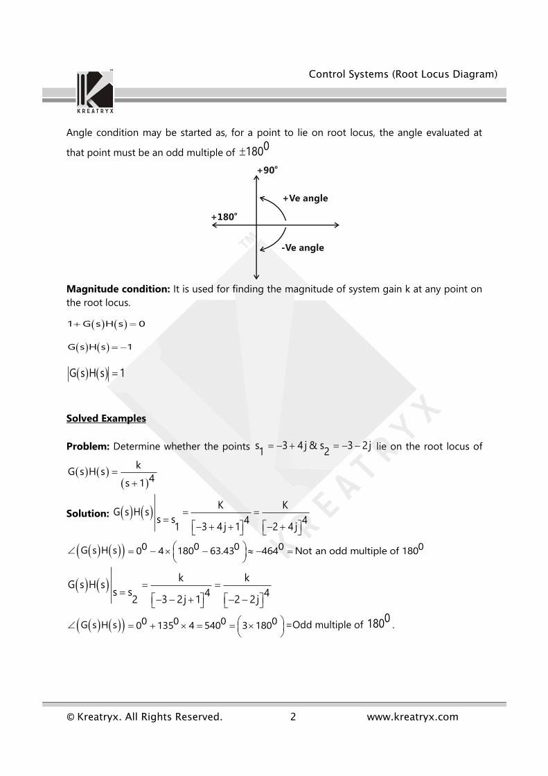
Angle condition may be started as, for a point to lie on root locus, the angle evaluated at

that point must be an odd multiple of 0180

Magnitude condition: It is used for finding the magnitude of system gain k at any point on

the root locus.

1 G s H s 0

G s H s 1

G s H s 1

Solved Examples

Problem: Determine whether the points s 3 4 j & s 3 2j1 2 lie on the root locus of

kG s H s

4s 1

Solution: K K

G s H ss s 4 4

3 4 j 1 2 4 j1

G s H s 0 0 0 0 00 4 180 63.43 464 Not an odd multiple of 180

k k

G s H ss s 4 4

3 2j 1 2 2 j2

G s H s 0 0 0 00 135 4 540 3 180

=Odd multiple of 0180 .



Advantages of Root Locus

The root locus is a powerful technique as it brings into focus the complete dynamic

response of the system and further, being a graphical technique, an approximate root locus

can be made quickly and designer can be easily visualize the effect of varies system

parameters an root location.

The root locus also provides a measure of sensitively of roots to the vacations in

parameters being considered.

It may further be pointed out here that root locus technique is applicable to single as well

as multiple loop system.

Construction Rules Of Root Locus

Rule 1: The root locus is symmetrical about real axis (G(s)H(s) = -1)

Rule 2: Each branch of Root Locus originates at an open loop pole and terminates at an

open loop zero or infinity.

Let P = number of open loop poles

Z = number of open loop zeroes

And if P > Z

Then,

No. of branches of root locus = P

No. of branches terminating at zeroes = Z

No. of branches terminating at infinity = (P – Z)

Rule 3: A point on real axis is said to be on root locus if to the right side of their point the

sum of number of open loop poles & zeroes is odd.

Ex:

k s 2 s 6G s

s s 4 s 8

P 3 ; Z 2 ; P Z 1

NRL – Not Root Locus; RL – Root Locus



Rule 4: Angle of asymptotes

The P – Z branches will terminate at infinity along certain straight lines known as asymptotes

of root locus.

Therefore, number of asymptotes = (P - Z)

Angle of asymptotes is given by:

02q 1 180; q 0,1,2,3.......

P Z

Suppose if P – Z = 2, then angle of asymptotes would be:

02 0 1 180 0901 2

and

2 1 10 0180 270

2 2

Solved Examples

Problem: Find the angle of asymptotes of a system whose characteristic equation is

2s s 4 s 2s 1 k s 1 0

Solution: The characteristic equation can be written in standard form as shown below:

K s 1

1 02s s 4 s 2s 1

K s 1G s H s

2s s 4 s 2s 1

P 4 ; Z 1 ; P Z 3

2 0 10 0180 60

1 3

2 1 10 0180 180

2 3

2 2 10 0180 300

3 3



Rule 5: Centroid

It is the intersection point of asymptotes on the real axis, it may or may not be a part of root

locus.

Realpart of openloop poles Realpart of openloop zeroescentroid

P Z

Solved Examples

Problem: Find centroid of the system whose characteristic equation is given as:

3 2s 5s K 6 s k 0

Solution: 3 2s 5s sk k 6s 0 => 3 2s 5s 6s k s 1 0

k s 1 k s 11

3 2 s s 2 s 3s 5s 6s

P = 3, Z = 2

Poles = 0, -2, -3 ; zeroes = -1

0 2 3 1centroid 2,0

3 1

Rule 6: Break Points

They are those points where multiple roots of the characteristics equation occur.

Procedure to find Break Points:

1. Construct 1 + G(s)H(s) = 0

2. Write k in terms of s

3. Find dk

0ds

4. The roots of dk

0ds

give the locations of break-away points.

5. To test the validity of breakaway points substitute in step – 2.

If k > 0, it means a valid breakaway point.



Breakaway Points

If the break point lies between two successive poles then it is termed as a Breakaway Point.

Predictions

1) The branches of root locus either approach or leave the breakaway points at an angle of

0180

n

Where n = no. of branches approaching or leaving breakaway point.

2) The complex conjugate path for the branches of root locus approaching or leaving or

breakaway points is a circle.

3) Whenever there are 2 adjacently placed poles on the real axis with the section of real axis

between there as part of RL, then there exists a breakaway point between the adjacently

placed poles.

Solved Examples

Problem: Plot Root Locus for the system shown below:

Solution: Applying Construction Rules of the Root Loci

C s k

2R s s 2s k

kG s

s s 2

Rule 2: P = 2, Z = 0, P – Z = 2

Rule 3: Section of real axis lying on Root Locus



Rule 4: 2 0 1 2 10 0 0180 90 ; 180 270

1 22 2

Rule 5: 0 2 0

centroid 12

Rule 6: Breakaway points

2s 2s k 0 => 2k s 2s

dk2s 2 0 s 1

ds

From the third prediction about Breakaway points we know that there must be a breakaway

point between s=0 and s=-2. Hence s= -1 is a valid breakaway point.

Since centroid and breakaway point coincide the branches of root locus will leave breakaway

point along the asymptotes.

Break – in points

The points where two branches of roots locus converge are called as break in points. A

Break-in Point lies between two successive zeroes.

To differentiate between break in & break away points.

2d k0

2ds For break in points

2d k0

2ds For break-away points



Otherwise by observation a breakaway point lies between two poles and a break-in point lies

between two zeroes.

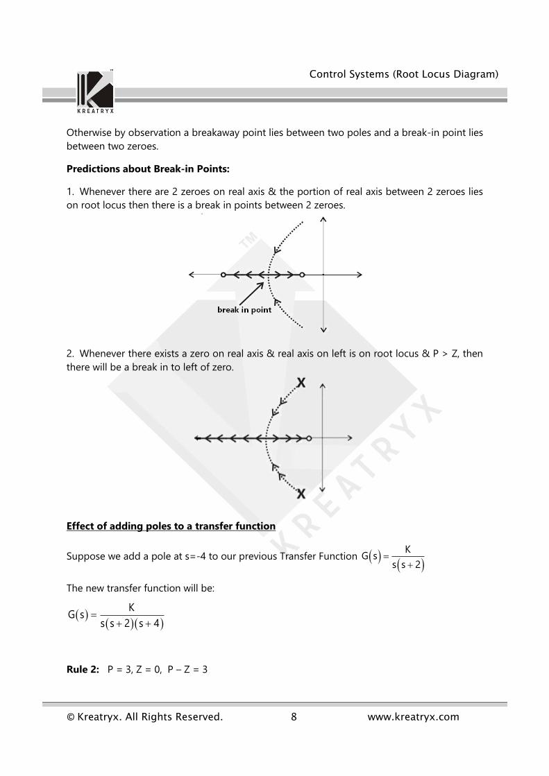
Predictions about Break-in Points:

1. Whenever there are 2 zeroes on real axis & the portion of real axis between 2 zeroes lies

on root locus then there is a break in points between 2 zeroes.

2. Whenever there exists a zero on real axis & real axis on left is on root locus & P > Z, then

there will be a break in to left of zero.

Effect of adding poles to a transfer function

Suppose we add a pole at s=-4 to our previous Transfer Function

KG s

s s 2

The new transfer function will be:

KG s

s s 2 s 4

Rule 2: P = 3, Z = 0, P – Z = 3



Rule 3: The sections of real axis lying on Root Locus is shown on right

Rule 4: 0 0 060 , 180 , 3001 2 3

Rule 5: Centroid

0 2 4 02

3 0

Rule 6: Break away points

Characteristic Equation: 3 2s 6s 8s K 0 =>

3 2K s 6s 8s

dK 23s 12s 8 0ds

23s 12s 8 0 s 0.845, 3.15

Since Breakaway point must lie between two successive poles that is it must lie between 0

and -2 so s=-0.845 is a valid breakaway point whereas s=-3.15 is invalid.

The root locus for this system is shown below,

Here, the root locus shifts towards right & hence stability decreases.



Effect of adding zeroes to a transfer function

Suppose we add a zero to the transfer function in the previous case at s= -1, then the

Transfer Function becomes:

K s 1G s

s s 2 s 4

Rule 2: P 3, Z 1, P Z 2

Rule 3: The sections of real axis lying on Root Locus are shown below:

Rule 4: 0 090 , 2701 2

Rule 5: 0 2 4 1

centroid 2.52

Rule 6: Breakaway point

Characteristic Equation of Closed Loop System is: 3 2s 6s 8s Ks K 0 =>

3 2s 6s 8sK

s 1

2

2 3 2s 1 3s 12s 8 s 6s 8sdk

0 s 2.9ds s 1



The branches originate at Breakaway Point and tend to infinity along the asymptotes.

Here, the root locus shifts towards left and hence stability increase.

Solved Examples

Problem: Draw Root Locus for the system whose open loop transfer function is

K s 2G s

s s 1

Solution: Applying Construction rules of the Root Loci

Rule 2: P 2, Z 1, P Z 1

Rule 3: The sections of real axis lying on Root Locus are shown below:

Rule 4: Angle of Aymptotes 0180

Rule 5: 0 1 2

centroid 11

Rule 6: Break away points

s s 1 K s 2 0 =>

2s sK

s 2

2s 2 2s 1 s s 1dk

0 02ds

s 2

2s 4s 2 0 => s 2 2 0.6, 3.4

Since, s = -0. Lie between two consecutive poles it is a Break away point and since s = -3.4

lies between a zero and infinity it is a break-in point.



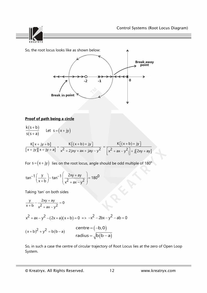
So, the root locus looks like as shown below:

Proof of path being a circle

k s b

s s a

Let s x jy

K x b jyK x jy b

2 2x jy x jy a x 2jxy ax jay y

K x b jy

2 2x ax y j 2xy ay

For s x jy lies on the root locus, angle should be odd multiple of 1800

y 2xy ay1 1 0tan tan 1802 2x b x ax y

Taking ‘tan’ on both sides

y 2xy ay0

2 2x b x ax y

2 2x ax y 2x a x b 0 => 2 2x 2bx y ab 0

2 2x b y b b a

centre b,0

radius b b a

So, in such a case the centre of circular trajectory of Root Locus lies at the zero of Open Loop

System.



Rule 7: Intersection of Root Locus with imaginary axis

Roots of auxiliary equation A(s) at k kmax

(i.e. Maximum value of Gain K for which the

closed loop system is Stable) from Routh Array gives the intersection of Root locus with

imaginary axis.

The value of k kmax

is obtained by equating the coefficient of s1 in the Routh Array to

zero.

Solved Examples

Problem: Find the intersection of root locus with the imaginary axis and also the intersection

of asymptotes with imaginary axis for the system whose open loop Transfer Function is given

by

kG s

s s 2 s 4

.

Solution: Characteristic Equation of the system is given as

3 2s 6s 8s k 0

Routh Array:

3s 1 8

2s 6 K

48 k1s6

0s K

For stability 48 k

0 k 486

& k 0

range 0 k 48

At k k 48max

2 2A s 6s k 0 6s 48 0

s j 8 j2.82



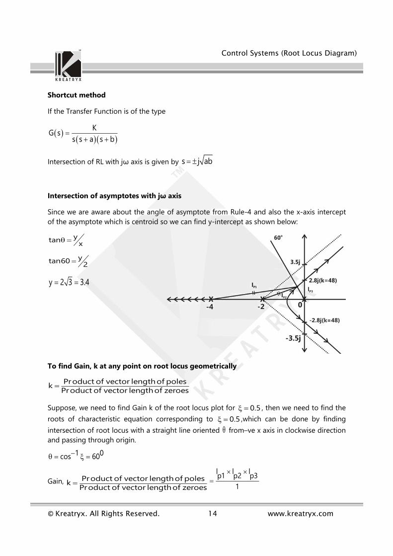
Shortcut method

If the Transfer Function is of the type

KG s

s s a s b

Intersection of RL with jω axis is given by s j ab

Intersection of asymptotes with jω axis

Since we are aware about the angle of asymptote from Rule-4 and also the x-axis intercept

of the asymptote which is centroid so we can find y-intercept as shown below:

ytanx

ytan602

y 2 3 3.4

To find Gain, k at any point on root locus geometrically

Product of vector lengthof polesk

Product of vector lengthof zeroes

Suppose, we need to find Gain k of the root locus plot for 0.5 , then we need to find the

roots of characteristic equation corresponding to 0.5 ,which can be done by finding

intersection of root locus with a straight line oriented from–ve x axis in clockwise direction

and passing through origin.

1 0cos 60

Gain, Product of vector lengthof polesk

Product of vector lengthof zeroes

l l lp1 p2 p3

1



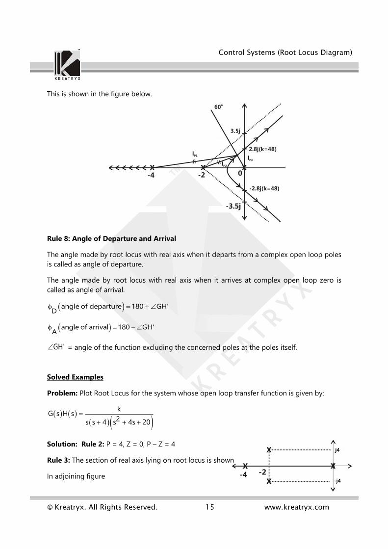
This is shown in the figure below.

Rule 8: Angle of Departure and Arrival

The angle made by root locus with real axis when it departs from a complex open loop poles

is called as angle of departure.

The angle made by root locus with real axis when it arrives at complex open loop zero is

called as angle of arrival.

angle of departure 180 GH'D

angle of arrival 180 GH'A

GH' = angle of the function excluding the concerned poles at the poles itself.

Solved Examples

Problem: Plot Root Locus for the system whose open loop transfer function is given by:

kG s H s

2s s 4 s 4s 20

Solution: Rule 2: P = 4, Z = 0, P – Z = 4

Rule 3: The section of real axis lying on root locus is shown

In adjoining figure



Rule 4: 0 0 0 045 , 135 , 225 , 3151 2 3 4

Rule 5: 0 2 2 4 0

centroid 24


4 3 2s 8s 36s 80s K 0

4 3 2K s 8s 36s 80s

dk0

ds =

3 24s 24s 72s 80 0 => s= 2, 2 j2.45

Note: To check validity of complex break point use angle criterion.

Rule 7: Routh Array

4s 1 36 K

3s 8 80 0

2s 26 K

2080 8k1s26

0s K

For stability 2080 8k

0 k 26026

& K > 0

range 0 k 260

For k=260 A.E.= 2A s 26s k 0

226s 260 0 => s j3.16

Intersection of asymptotes with jω – axis

y tan45 2 j2



Rule 8: Angle of departure

4 01180 tanp1 0 2

1180 tan 2 0116.56

090p2

4 01tan 63.4p3 2 4

0

z p

Sum of Angles from zeroes - Sum of Angles from Poles

180 180 116.6 90 63.4D

0180 270 90

Else

KG s H s

s 2 4 j s s 4 s 2 4 j s 2 4 j

K

2 4 j 2 4 j 8 j

GH' 4 41 1 0tan tan 902 2

1 1 04 4180 tan tan 902 2

= 270

0180 270 90D

So, the root locus of the system looks like as shown below:



Problem: Plot Root Locus for the system whose Open Loop Transfer Function is given by

2k s 2s 5G s

s 2 s 0.5

Solution: Rule 2: P = 2, Z = 2, P – Z = 0

Rule 3: The section of real axis lying on Root Locus is shown below:

Since P-Z = 0, Rule 4 and Rule 5 are of no use as there are no asymptotes.


Characteristic Equation of the system is:

2s 2 s 0.5 k s 2s 5 0 =>

2s 1.5s 1k

2s 2s 5

dk0

ds => s 0.4, 3.6

Here, since Breakaway point must lie between two consecutive poles so s = -0.4 is a valid

Breakaway Pont whereas s = 3.6 is an invalid point.

Rule 7: 2s 1 k s 1.5 2k 5k 1 0

Routh Array:

2s 1 k 5k 1

1s 1.5 2k 0

0s 5k 1 0

For stability 1 k 0 k 1 & 1.5 2k 0 k 0.75 & 5k 1 0 k 0.2

range 0.2 k 0.75



k k 0.75max

A.E. = 2A s 1 k s 5k 1 21.75s 5 0.75 1 0

s j1.25

Rule 8: Angle of arrival

k s 1 2 j s 1 2 jG s

s 2 s 0.5

at s 1 2jA

1 2j 1 2j 1 1 12 2GH' tan 4 j tan tan

3 0.53 2j 0.5 2j

GH' 20 1 190 tan tan 43

0 0 0 090 76 34 20

0 0 0180 20 200

The Root Locus for the system looks like as shown below:



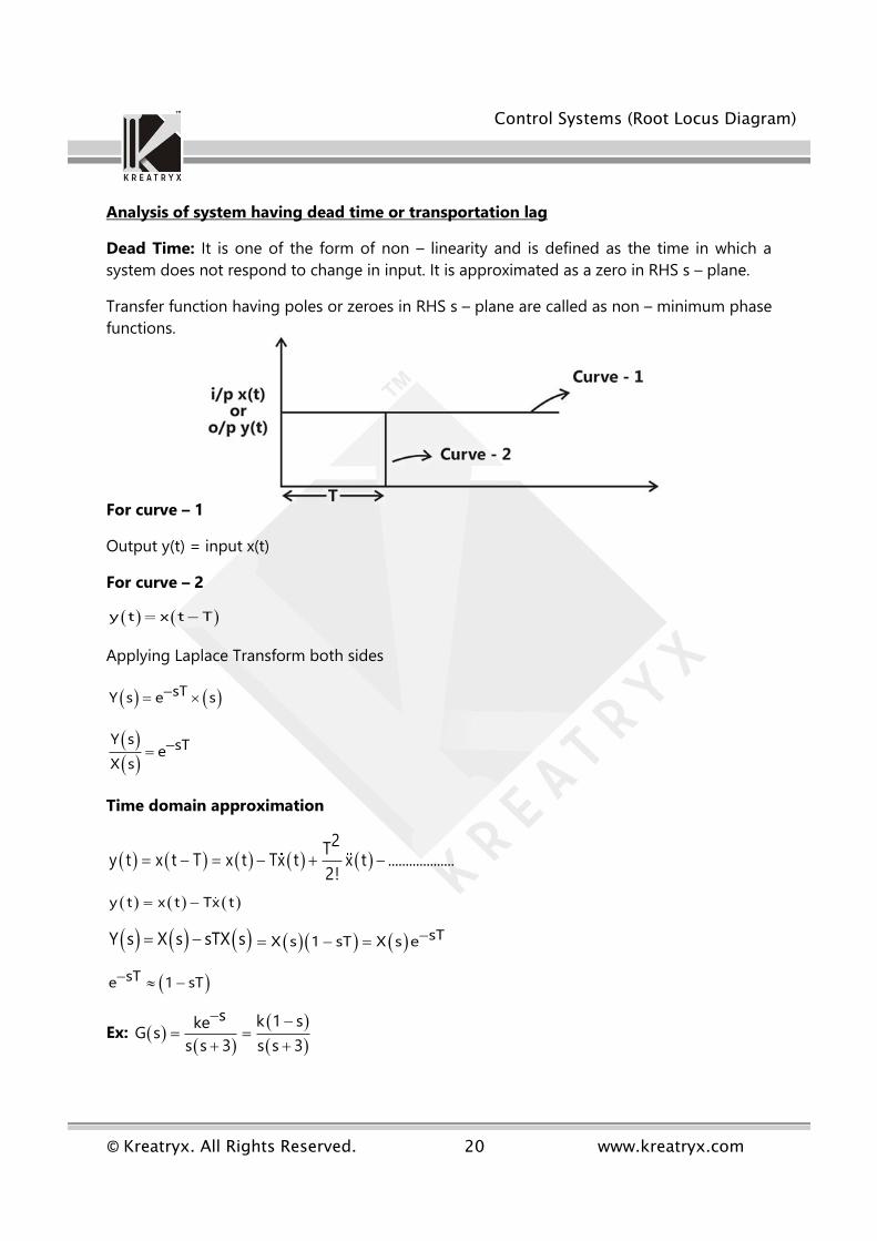
Analysis of system having dead time or transportation lag

Dead Time: It is one of the form of non – linearity and is defined as the time in which a

system does not respond to change in input. It is approximated as a zero in RHS s – plane.

Transfer function having poles or zeroes in RHS s – plane are called as non – minimum phase

functions.

For curve – 1

Output y(t) = input x(t)

For curve – 2

y t x t T

Applying Laplace Transform both sides

sTY s e s

Y s sTeX s

Time domain approximation

2T

y t x t T x t Tx t x t ...................2!

y t x t Tx t

Y s X s sTX s sTX s 1 sT X s e

sTe 1 sT

Ex:

s k 1 skeG s

s s 3 s s 3



Complimentary Root Locus (CRL)

Angle Condition:

0 0G s H s 0 2q 180

Magnitude Condition:

G s H s 1

Construction Rules

Rule 1: The CRL is symmetrical about real axis G s H s 1

Rule 2: Number of branches terminating at infinity is (P – Z).

Rule 3: A point on real axis is said to be on CRL if to the right side of the point the sum of

open loop poles & zeroes is even.

Rule 4: Angle of asymptotes

02q 180

P Z

, q 1,2,3................

Rule 5: Centroid: same as Root locus

Rule 6: Break point: Same as RL

Rule 7: Intersection of CRL with jω axis same as root locus.

Rule 8: Angle of departure & arrival.

0D

0A

Where GH'Z P

Solved Examples

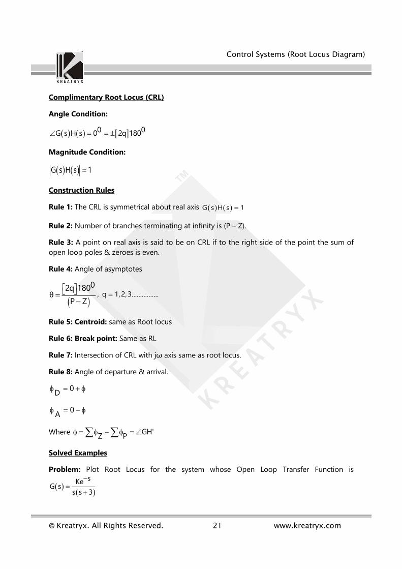
Problem: Plot Root Locus for the system whose Open Loop Transfer Function is

sKeG s

s s 3



Solution:

k 1 s k s 1G s

s s 3 s s 3

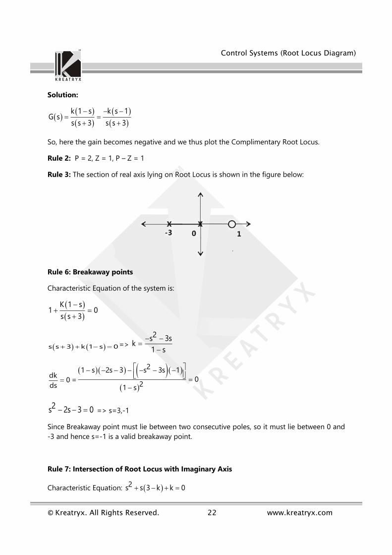
So, here the gain becomes negative and we thus plot the Complimentary Root Locus.

Rule 2: P = 2, Z = 1, P – Z = 1

Rule 3: The section of real axis lying on Root Locus is shown in the figure below:


Characteristic Equation of the system is:

K 1 s1 0

s s 3

s s 3 k 1 s 0 =>

2s 3sk

1 s

dk0

ds =

21 s 2s 3 s 3s 1

021 s

2s 2s 3 0 => s=3,-1

Since Breakaway point must lie between two consecutive poles, so it must lie between 0 and

-3 and hence s=-1 is a valid breakaway point.

Rule 7: Intersection of Root Locus with Imaginary Axis

Characteristic Equation: 2s s 3 k k 0



Routh Array:

2s 1 k

1s 3 k 0

0s k

For stability 3-k>0 => k<3 & k>0

Range 0<k<3

k k 3max

A.E.= 2A s s k 0

s j1.732

Root Contours

Root contours are multiple root locus diagrams obtained by varying multiple parameters in a

transfer function diagram in same s – plane.

k sG s H s

s s 1 s 8

Case 1: let 0 , and gain K is varied

kG s

s 1 s 8



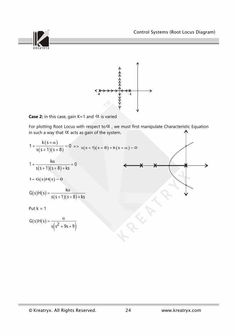
Case 2: In this case, gain K=1 and is varied

For plotting Root Locus with respect to , we must first manipulate Characteristic Equation

in such a way that acts as gain of the system.

k s1 0

s s 1 s 8

=> s s 1 s 8 k s 0

k1 0

s s 1 s 8 ks

1 G s H s 0

kG s H s

s s 1 s 8 ks

Put k = 1

G s H s

2s s 9s 9

Root Locus Diagram · Rule 1: The root locus is symmetrical about real axis (G(s)H(s) = -1) Rule 2:...

Documents

Transcript of Root Locus Diagram · Rule 1: The root locus is symmetrical about real axis (G(s)H(s) = -1) Rule 2:...