XMUT315 Control System Engineering

Root Locus Construction

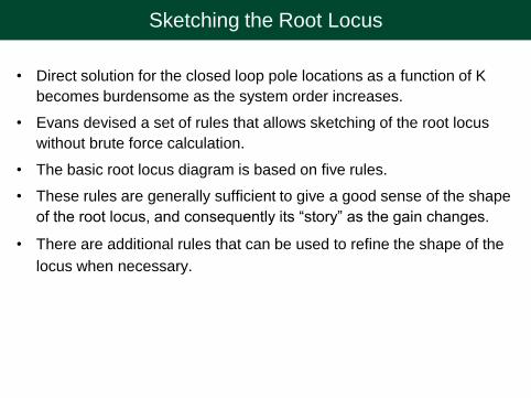
Sketching the Root Locus

• Direct solution for the closed loop pole locations as a function of K

becomes burdensome as the system order increases.

• Evans devised a set of rules that allows sketching of the root locus

without brute force calculation.

• The basic root locus diagram is based on five rules.

• These rules are generally sufficient to give a good sense of the shape

of the root locus, and consequently its “story” as the gain changes.

• There are additional rules that can be used to refine the shape of the

locus when necessary.

Rule #1 for Sketching a Root Locus

The number of branches of the root locus is equal to the number of closed

loop poles.

• A “branch” is a segment of the root locus traversed by a single pole

as the gain is varied.

• This rule implies that there is one and only one branch originating at

each pole.

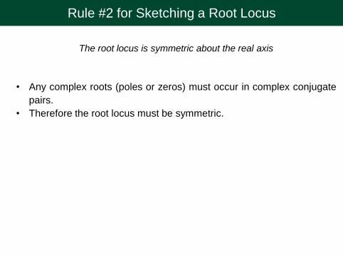
Rule #2 for Sketching a Root Locus

The root locus is symmetric about the real axis

• Any complex roots (poles or zeros) must occur in complex conjugate

pairs.

• Therefore the root locus must be symmetric.

Rule #3 for Sketching a Root Locus

A branch of the RL will only be on the real axis to the left of an odd number of

finite open loop roots.

• Recall that roots means both poles and zeros!

• As discussed earlier, the solution of the characteristic equation

implies that CG = -180° at all points on the root locus.

• Now, all roots on the further left than a test point will contribute no

phase shift.

• However, both zeros and poles to the right of a test point contribute

180°.

• We therefore only satisfy the characteristic equation if there is an odd

number of roots on the real axis that are further to the right than our

test point.

Rule #4 for Sketching a Root Locus

The root locus begins at the finite and infinite poles of C(s)G(s) and ends at

the finite and infinite zeros of C(s)G(s).

• Let’s calculate what happens to T = KCG/(1+KCG) for very small and

very large values of K.

• Note that we have allowed for more interesting compensators here, by

expanding the previous C into KC, where C now contains any

compensator roots.

• lim k->0 T(s) = KCG/1, therefore the poles of T for small K are the poles

of CG. That is, the poles of T start at the open loop poles of the plant

and the open loop poles of the compensator.

• lim k-> T(s) = KCG/KCG, therefore the poles of T for large K are the

roots of CG. These are the zeros of CG, which is just the combination

of the zeros of C and the zeros of G.

Rule #5 for Sketching a Root Locus

The root locus approaches straight line asymptotes as the gain approaches

infinity. The real-axis intercept, a, and angles, a, are given by

where P is the number of finite poles,

Z is the number of finite zeros, pi is the

i-th pole, zi is the i-th zero and k Z.

• In general, a root locus will have P-Z

asymptotes, so you will need to

substitute P-Z consecutive values for k

into the a equation.

Example #1

• Sketch the root locus of the transfer function

T (s) =s + 3

s(s + 1)(s + 2)(s + 4)

• We have open loop poles at s = 0,-1,-2 and -4 and an open loop zero

at s = -3.

• Let’s first determine the parameters of the asymptotes. First, the

departure point:

Example #1

• We can therefore sketch in the asymptotes.

• Work on the angle of the asymptotes:

Example #1

• With the asymptotes in place we can sketch in the various branches

of the root locus.

• R1: We expect four branches to

the locus.

• R3: The locus will pass along

the real axis between the

slowest two poles and between

the third slowest pole and the

zero.

• There will also be a branch on

the real axis beyond the fastest

pole.

Root Locus

Exercise #1

G(s) =s2 - 4 s + 20

(s + 2)(s + 4)

Exercise #2

G(s) = 1

s [(s + 4)2 + 16]

Exercise #3

G(s) =1 + s

s2

Exercise #4

G(s) =1

s(s + 2 )[(s + 1)2 + 4]

Refining the Root Locus

There are many features of the root locus as yet undetermined.

• Where do pole pairs break away / break into the real axis?

• Where do pole pairs cross the imaginary axis?

• At what angles do pole pairs depart from the open loop poles

and enter open loop zeros?

We have two options for determining these factors:

• Use Matlab (or some other tool),

• Apply some more rules.

Pole Break-away / Break-in Angles

• We often encounter systems where poles break away from the real

axis into the complex plane, or conversely merge back into the plane.

• The angle at which the poles leave the plane is given by 180/n where

n is the number of poles breaking away/in.

• Typically n = 2, so the angle of departure/arrival from the real axis is

90°.

Pole Break-away / Break-in Locations

• We know that a break-away occurs as gain is increasing. Therefore,

the break-away point has the highest gain of any point where the

locus is on the real axis (in cases where there are multiple segments

on the real axis it might not be the highest gain globally, but it will be a

local maximum).

• Similarly around a break-in point, the locus first touches the real axis

at some value of gain. The locus then continues on the real axis as

the gain increases. The break-in point will therefore correspond to a

local minimum of gain.

• We know that the root locus satisfies the characteristic equation 1 +

KG = 0. Thus everywhere along the root locus, K = -1/G(s) . Along

the real axis we know that s is real, so we can write s = . Hence K

= -G() on the real axis.

Pole Break-away / Break-in Location Example

G(s) =(s - 3)(s - 5)

(s + 1)(s + 2)

Root Locus

Real Axis

• Along the root locus, KG = -1K (s - 3 )(s - 5)

= -1.(s + 1)(s + 2)

• We are considering gains only on the real axis, hence we substitute s=.

K ( - 3 )( - 5)

( + 1)( + 2)= 1

2 + 3 + 2 2

- 8 + 15

• We can solve for K and obtain

Pole Break-away / Break-in Location Example

• We want to find local extrema in the K value. We can find extrema by

finding the derivative of the expression for K and setting it to zero.

• Now solve dK/d = 0 = 11 b + 26b + 61 using the quadratic equation

to find the critical values of a. We find that ab = -1.45, 3.82

• Thus, the breakaway point is at s = -1.45 and the break-in point is at s

= 3.82.

Pole Break-away / Break-in Locations

• There is also an easier, though less obvious technique.

Breakaway and Break-in points, s = ab, satisfy the relationship

• where pi and zi are the pole and zero values of CG, where we have

Z total zeros and P total poles.

• For our example, we get

• After some algebra we get 112 + 26 + 61 = 0 as before. We can

complete the problem as earlier.

Imaginary Axis Crossings

• The gain K at which the root locus crosses the imaginary axis is the

value at which the system becomes unstable (stable systems cannot

have poles in the right half of the s-plane).

• There is no easy way to use the Root Locus to find this point; if you

need to calculate the crossing point then perform a Routh-Hurwitz

test.

Angles of Departure and Arrival at Complex Roots

• Recall that at all points on a root locus we satisfy the characteristic

equation, 1 + CG = 0.

• Now, the angle (phase) of CG is the sum of the phases of the poles

and zeros that make up CG.

• That is, to be on the root locus the sum of the angles to the closed

loop roots is always -180°.

Angles of Departure and Arrival at Complex Roots

• Now, let us presume that we are on a point an arbitrarily small

distance, , away from a system root.

• We can assume that the angle from each of the other roots to our test

point is the same as from that root to the root of interest.

• We can calculate these other angles directly, enabling us to find the

angle from e to the root of departure or arrival.

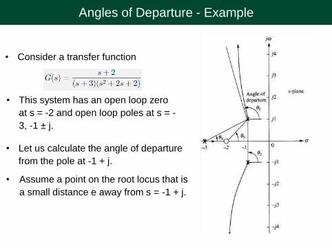
Angles of Departure - Example

• Consider a transfer function

• This system has an open loop zero

at s = -2 and open loop poles at s = -

3, -1 ± j.

• Let us calculate the angle of departure

from the pole at -1 + j.

• Assume a point on the root locus that is

a small distance e away from s = -1 + j.

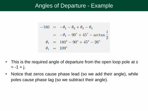
Angles of Departure - Example

• This is the required angle of departure from the open loop pole at s

= -1 + j.

• Notice that zeros cause phase lead (so we add their angle), while

poles cause phase lag (so we subtract their angle).