arX

iv:0

706.

3897

v1 [

quan

t-ph

] 2

6 Ju

n 20

07

Romanovski Polynomials in Selected Physics Problems

A. P. Raposo1, H. J. Weber2, D. Alvarez-Castillo3, M. Kirchbach3,

1Facultad de Ciencias, Av. Salvador Nava s/n, San Luis Potosı,

S.L.P. 78290, Universidad Autonoma de San Luis Potosı, Mexico,

2Department of Physics, University of Virginia,

Charlottesville, VA 22904, USA and

3 Instituto de Fısica, Av. Manuel Nava 6, San Luis Potosı,

S.L.P. 78290, Universidad Autonoma de San Luis Potosı, Mexico

(Dated: May 30, 2018)

Abstract

We briefly review the five possible real polynomial solutions of hypergeometric differential equa-

tions. Three of them are the well known classical orthogonal polynomials, but the other two are

different with respect to their orthogonality properties. We then focus on the family of polynomials

which exhibits a finite orthogonality. This family, to be referred to as the Romanovski polynomi-

als, is required in exact solutions of several physics problems ranging from quantum mechanics and

quark physics to random matrix theory. It appears timely to draw attention to it by the present

study. Our survey also includes several new observations on the orthogonality properties of the

Romanovski polynomials and new developments from their Rodrigues formula.

1

I. INTRODUCTION

Several physics problems ranging from ordinary–and supersymmetric quantum mechan-

ics to applications of random matrix theory in nuclear and condensed matter physics are

ordinarily resolved in terms of Jacobi polynomials of purely imaginary arguments and param-

eters that are complex conjugate to each other. Depending on whether the degree n of these

polynomials is even or odd, they appear either genuinely real or purely imaginary. The fact

is that all the above problems are naturally resolved in terms of manifestly real orthogonal

polynomials. These real polynomials happen to be related to the above Jacobi polynomials

by the purely imaginary phase factor, in, much like the phase relationship between the hy-

perbolic and the trigonometric functions, i.e. sin ix = i sinh x. These polynomials have first

been reported by Sir Edward John Routh [1] in 1884, and then were rediscovered within the

context of probability distributions by Vsevolod Romanovski [2] in 1929. They are known

in the mathematics literature under the name of “Romanovski” polynomials.

Romanovski polynomials may be derived as the polynomial solutions of the ODE

(1 + x2)d2R(x)

dx2+ t(x)

dR(x)

dx+ λR(x) = 0, (1)

with t(x) a polynomial, at most a linear, which is a particular subclass of the hypergeometric

differential equations [3], [4]. Other subclasses give rise to the well known classical orthogonal

polynomials of Hermite, Laguerre and Jacobi [4], [5]. Romanovski polynomials are not so

widespread as the others in applications. But in recent years several problems have been

solved in terms of this family of polynomials (Schrodinger equation with the hyperbolic

Scarf and the trigonometric Rosen-Morse potentials [6, 7], Klein-Gordon equation with equal

vector and scalar potentials [8], certain classes of non-central potential problems as well [9])

and so they deserve a closer look and be placed on equal footing with the classical orthogonal

polynomials.

In this context, our goal is threefold. First of all, it is to establish the orthogonality

properties of these polynomials. This is achieved by the same methods as for any other

hypergeometric differential equation. Our second goal is to explain their use as orthogonal

eigenfunctions of some Hamiltonian operators. Third, Eq. (1) has been described in [10] as

a complexification of the Jacobi ODE, a general expression that can be written as

(1− x2)d2P (x)

dx2+ t(x)

dP (x)

dx+ λP (x) = 0, (2)

2

where t(x) is again an arbitrary polynomial of at most first degree, but not necessarily the

same as in Eq. (1). If that were the case, solutions to Eq. (1) would be the complexification

of the solutions to Eq. (2), that is, the complexification of the Jacobi polynomials. Hence,

our final goal is to clarify this relationship.

We deal with all these issues in the following way: In Section II we give a classification

of hypergeometric equations placing Eq. (1) among them. Next, in Section III we show

some expected properties of the R(α,β)n (x) functions as solutions of a hypergeometric ODE

such as: being indeed polynomials, recurrence relations; and the absence of another, namely

general orthogonality. In Section IV we compare the polynomials R(α,β)n (x) with the com-

plexified Jacobi polynomials. In Section V we show some examples of physical problems

whose solutions lead to Romanovski polynomials. Section VI sheds light on some peculiar-

ities of orthogonal polynomials as part of quantum mechanics wave functions. In the final

Section VII we summarize our conclusions.

II. CLASSIFICATION OF HYPERGEOMETRIC DIFFERENTIAL EQUATIONS

A hypergeometric equation [3] is an ODE of the form

s(x)F ′′(x) + t(x)F ′(x) + λF (x) = 0, (3)

where the unknown is a real function of real variable F : U → R, where U ⊂ R is some

open subset of the real line, and λ ∈ R a corresponding eigenvalue, and where the functions

s and t are real polynomials of at most second order and first order, respectively. Here the

prime stands for differentiation with respect to the variable x. This class of ODEs is very

well known both from the mathematical and the physical points of view. From the mathe-

matical one, many properties that its solutions exhibit make them interesting in their own

right. For instance, the classical orthogonal polynomials [3], [11], [12] (Hermite, Laguerre

and Jacobi polynomials, the latter including as particular cases Legendre, Chebyshev and

Gegenbauer polynomials) are solutions of particular subfamilies of hypergeometric ODEs.

From the physical point of view, many of the exact solutions to the eigenvalue equation of

a quantum mechanical Hamilton operator lead to an equation of the hypergeometric kind:

harmonic oscillator, Coulomb potential, the trigonometric Rosen-Morse and Scarf potentials,

hyperbolic Rosen-Morse and hyperbolic Scarf potentials.

3

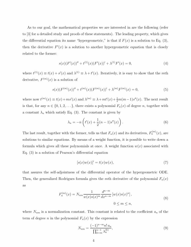
As to our goal, the mathematical properties we are interested in are the following (refer

to [3] for a detailed study and proofs of these statements). The leading property, which gives

the differential equation its name “hypergeometric,” is that if F (x) is a solution to Eq. (3),

then the derivative F ′(x) is a solution to another hypergeometric equation that is closely

related to the former:

s(x)(F ′(x))′′ + t(1)(x)(F ′(x))′ + λ(1)F ′(x) = 0, (4)

where t(1)(x) ≡ t(x) + s′(x) and λ(1) ≡ λ+ t′(x). Iteratively, it is easy to show that the mth

derivative, F (m)(x) is a solution of

s(x)(F (m)(x))′′ + t(m)(x)(F (m)(x))′ + λ(m)F (m)(x) = 0, (5)

where now t(m)(x) ≡ t(x)+ms′(x) and λ(m) ≡ λ+mt′(x)+ 12m(m−1)s′′(x). The next result

is that, for any n ∈ {0, 1, 2, . . .}, there exists a polynomial Fn(x) of degree n, together with

a constant λn which satisfy Eq. (3). The constant is given by

λn = −n(t′(x) +

1

2(n− 1)s′′(x)

). (6)

The last result, together with the former, tells us that Fn(x) and its derivatives, F(m)n (x), are

solutions to similar equations. By means of a weight function, it is possible to write down a

formula which gives all these polynomials at once. A weight function w(x) associated with

Eq. (3) is a solution of Pearson’s differential equation

[s(x)w(x)]′ = t(x)w(x), (7)

that assures the self-adjointness of the differential operator of the hypergeometric ODE.

Then, the generalized Rodrigues formula gives the mth derivative of the polynomial Fn(x)

as

F (m)n (x) = Nnm

1

w(x)s(x)mdn−m

dxn−m[w(x)s(x)n] ,

0 ≤ m ≤ n,

(8)

where Nnm is a normalization constant. This constant is related to the coefficient an of the

term of degree n in the polynomial Fn(x) by the expression

Nnm =(−1)n−mn! an∏n−1

k=m λ(k)n

, (9)

4

which is valid for 0 ≤ m ≤ n − 1 and n ≥ 1. Equation (8), with m = 0, gives the classical

Rodrigues formula

Fn(x) = Nn1

w(x)

dn

dxn[w(x)s(x)n] , (10)

where we have identified F(0)n (x) = Fn(x) and Nn0 = Nn.

If the functions s(x) and w(x) satisfy yet another condition, namely both being positive

within an interval (a, b) and

limx→a

s(x)w(x)xl − limx→b

s(x)w(x)xl = 0 , (11)

for any nonnegative integer l, then the family of polynomials is orthogonal with respect to

the weight function w, i.e.∫ b

a

w(x)Fm(x)Fn(x) dx = (fn)2δmn,

∀m,n ∈ {0, 1, 2, . . .},(12)

where fn is the norm of the polynomials. Hence, all hypergeometric ODEs admit a family

of polynomial solutions. But this family is not orthogonal for all hypergeometric ODEs.

The fact that a solution F (x) and its derivatives F (m)(x) obey hypergeometric ODEs

with the same coefficient s(x), Eqs. (3) and (5), suggests a classification in terms of the

polynomial s(x). Moreover, a classification according to the roots of s(x) has proved useful

and provides a characterization of the solutions [3],[4],[5]. There are five classes in this

scheme, as s(x) may be a constant, a first degree polynomial or a second order one with

two distinct real roots, one real root or, finally, two complex conjugate, not real, roots. In

addition, it is useful to note that an affine change of variable (i.e., x → a x + b, a 6= 0)

does preserve the hypergeometric character of Eq. (3) and the kind of roots of polynomial

s(x). Then, in each class, we may consider only a canonical form of the equation, to which

any other can be reduced by an affine change of the independent variable.

1. Polynomial s(x) is a constant:

We take as canonical form

H ′′(x)− 2αxH ′(x) + λH(x) = 0, (13)

where α ∈ R is an arbitrary constant, i.e., we have here a one-parameter family of ODEs.

We call it generalized Hermite equation (the equation with α = 1 is called Hermite equa-

tion). The polynomials are a generalization of Hermite polynomials, denoted {H(α)n },

5

n ∈ {0, 1, 2, . . .}. The weight function is

w(x) = e−αx2

. (14)

For α > 0 the additional conditions for orthogonality, Eq. (11), are fulfilled in the interval

(−∞,∞), hence we get an orthogonality relation:∫ ∞

−∞

e−αx2

H(α)m (x)H(α)

n (x) dx = (hn)2δmn,

∀m,n ∈ {0, 1, 2, . . . }, α > 0.

(15)

2. Polynomial s(x) is of the first degree:

The canonical form of the ODE is

xL′′(x) + t(x)L′(x) + λL(x) = 0, (16)

which we call generalized Laguerre equation. The first-order polynomial t is still arbitrary,

so this is a two-parameter family of ODEs. If t(x) is written as t(x) = −αx + β + 1, with

α, β ∈ R, the parameters (actually, Eq. (16) is called associated Laguerre equation in the

case α = 1, and Laguerre equation if α = 1 and β = 0), then the weight function is

w(x) = xβe−αx, (17)

and the polynomials are written {L(α,β)n }, n ∈ {0, 1, 2, . . .}. If α, β > 0, the condition of

Eq. (11) is fulfilled and one gets orthogonality in the interval [0,∞) as∫ ∞

0

xβe−αxL(α,β)m (x)L(α,β)

n (x) dx = (ln)2δmn,

∀m,n ∈ {0, 1, 2, . . . }, α, β > 0.

(18)

3. Polynomial s(x) is of the second degree, with two different real roots:

The canonical form of the ODE is

(1− x2)P ′′(x) + t(x)P ′(x) + λP (x) = 0, (19)

which is known as Jacobi equation. It is customary to write the arbitrary polynomial t(x)

in the form t(x) = β−α− (α+ β+2)x, where α, β ∈ R are the parameters. Then, for each

pair (α, β), the Rodrigues formula defines a family of polynomials, the Jacobi polynomials,

denoted {P (α,β)n }, n ∈ {0, 1, 2, . . . } with the weight function given by

w(x) = (1− x)α(1 + x)β . (20)

6

If parameters α and β satisfy α, β > −1, the additional condition of Eq. (11) is fulfilled in

the interval (−1, 1), so there is an orthonormalization relation:

∫ 1

−1

(1− x)α(1 + x)βP (α,β)m (x)P (α,β)

n (x) dx = (pn)2δmn,

∀m,n ∈ {0, 1, 2, . . . }, α, β > −1.

(21)

Some particular cases received special names: Gegenbauer polynomials if α = β, Chebyshev

I and II if α = β = ±1/2, Legendre polynomials if α = β = 0.

4. Polynomial s(x) is of the second degree, with one double real root:

We choose as canonical form of the ODE

x2B′′(x) + t(x)B′(x) + λB(x) = 0, (22)

If the arbitrary first order polynomial is written as t(x) = (α + 2)x+ β, with α, β ∈ R the

parameters, then the weight function is

w(α,β)(x) = xαe−β

x . (23)

We write the polynomials as {B(α,β)n }, n ∈ {0, 1, 2, . . . }, which are called Bessel polynomials

[13] (they were also given under type V in Ref. [2] and classified in Ref. [4]). There is

no combination of any particular values of the parameters and any interval which satisfies

Eq. (11), so neither of these families is orthogonal with respect to the weight function (23).

5. Polynomial s(x) is of the second degree, with two complex roots:

The canonical form of the ODE for this case is chosen as

(1 + x2)R′′(x) + t(x)R′(x) + λR(x) = 0, (24)

which is the one studied in [4]–[6], and [14]–[15]. A note of caution: the solutions introduced

in [6] and [7] seem to be different, but this is due just to a different form given to the

arbitrary polynomial t(x). A careful review shows that both papers are dealing with the

same ODE, namely Eq. (24), so the solutions must be the same up to a constant factor.

Writing the polynomial t(x) as t(x) = 2βx + α, with α, β ∈ R, we have again a two-

parameter family of ODEs with their respective families of polynomials which we denote

{R(α,β)n }, n ∈ {0, 1, 2, . . .}. With this notation (which differs slightly from [6],[7],[16]) the

weight function is

w(α,β)(x) = (1 + x2)β−1e−α cot−1 x. (25)

7

Upon comparison with Romanovski’s original work [2], we conclude {R(α,β)n } are the Ro-

manovski polynomials. In Section III we study the properties of these polynomials.

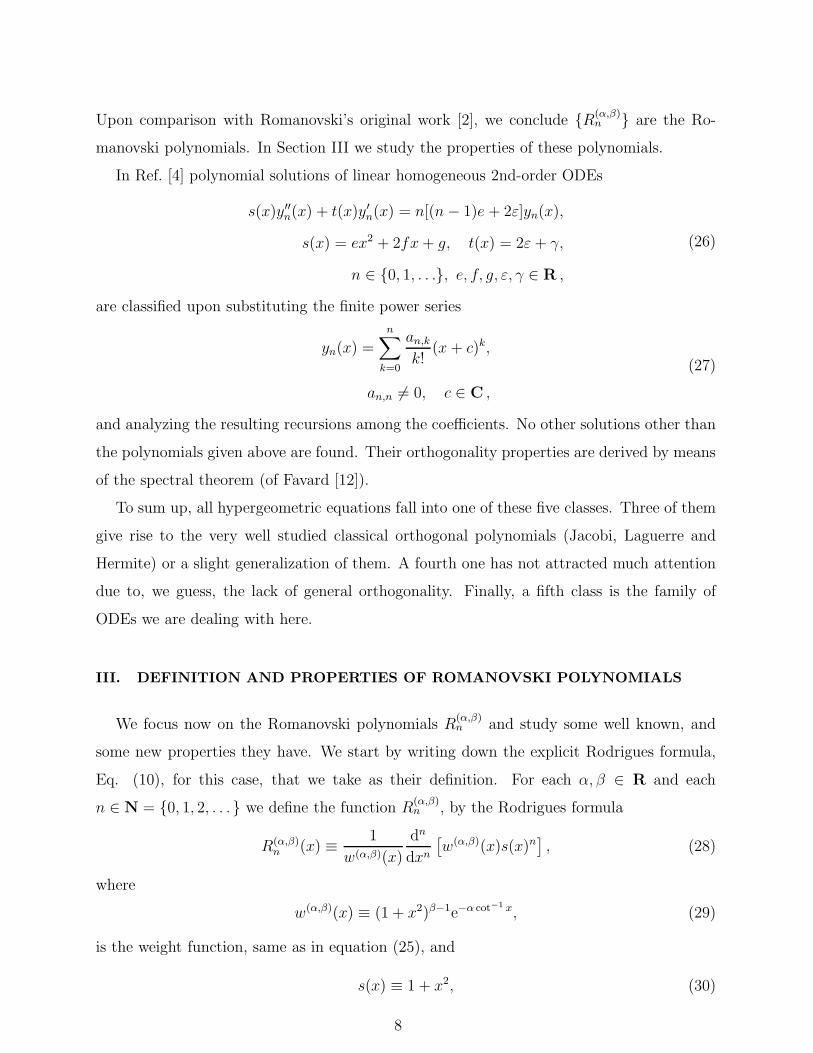
In Ref. [4] polynomial solutions of linear homogeneous 2nd-order ODEs

s(x)y′′n(x) + t(x)y′n(x) = n[(n− 1)e + 2ε]yn(x),

s(x) = ex2 + 2fx+ g, t(x) = 2ε+ γ,

n ∈ {0, 1, . . .}, e, f, g, ε, γ ∈ R ,

(26)

are classified upon substituting the finite power series

yn(x) =

n∑

k=0

an,kk!

(x+ c)k,

an,n 6= 0, c ∈ C ,

(27)

and analyzing the resulting recursions among the coefficients. No other solutions other than

the polynomials given above are found. Their orthogonality properties are derived by means

of the spectral theorem (of Favard [12]).

To sum up, all hypergeometric equations fall into one of these five classes. Three of them

give rise to the very well studied classical orthogonal polynomials (Jacobi, Laguerre and

Hermite) or a slight generalization of them. A fourth one has not attracted much attention

due to, we guess, the lack of general orthogonality. Finally, a fifth class is the family of

ODEs we are dealing with here.

III. DEFINITION AND PROPERTIES OF ROMANOVSKI POLYNOMIALS

We focus now on the Romanovski polynomials R(α,β)n and study some well known, and

some new properties they have. We start by writing down the explicit Rodrigues formula,

Eq. (10), for this case, that we take as their definition. For each α, β ∈ R and each

n ∈ N = {0, 1, 2, . . .} we define the function R(α,β)n , by the Rodrigues formula

R(α,β)n (x) ≡ 1

w(α,β)(x)

dn

dxn[w(α,β)(x)s(x)n

], (28)

where

w(α,β)(x) ≡ (1 + x2)β−1e−α cot−1 x, (29)

is the weight function, same as in equation (25), and

s(x) ≡ 1 + x2, (30)

8

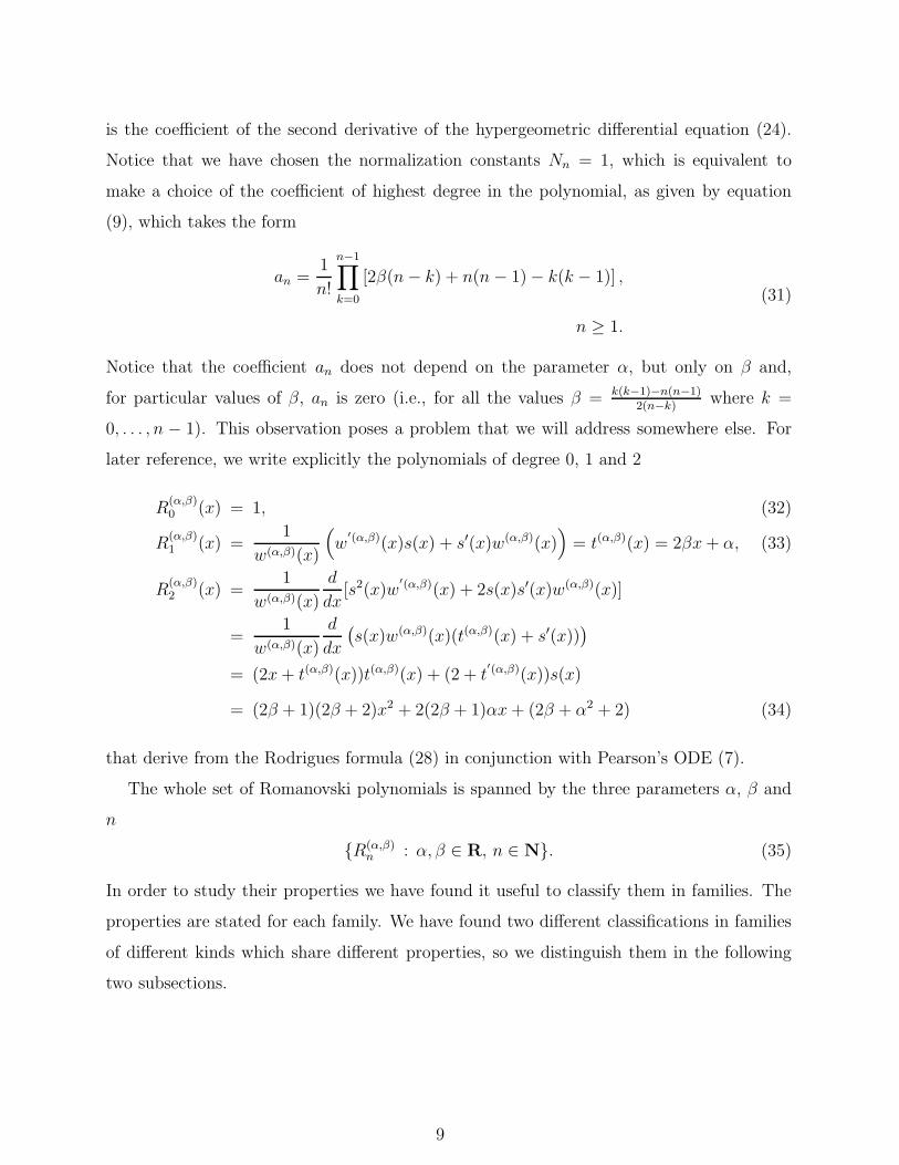
is the coefficient of the second derivative of the hypergeometric differential equation (24).

Notice that we have chosen the normalization constants Nn = 1, which is equivalent to

make a choice of the coefficient of highest degree in the polynomial, as given by equation

(9), which takes the form

an =1

n!

n−1∏

k=0

[2β(n− k) + n(n− 1)− k(k − 1)] ,

n ≥ 1.

(31)

Notice that the coefficient an does not depend on the parameter α, but only on β and,

for particular values of β, an is zero (i.e., for all the values β = k(k−1)−n(n−1)2(n−k)

where k =

0, . . . , n − 1). This observation poses a problem that we will address somewhere else. For

later reference, we write explicitly the polynomials of degree 0, 1 and 2

R(α,β)0 (x) = 1, (32)

R(α,β)1 (x) =

1

w(α,β)(x)

(w

′(α,β)(x)s(x) + s′(x)w(α,β)(x))= t(α,β)(x) = 2βx+ α, (33)

R(α,β)2 (x) =

1

w(α,β)(x)

d

dx[s2(x)w

′(α,β)(x) + 2s(x)s′(x)w(α,β)(x)]

=1

w(α,β)(x)

d

dx

(s(x)w(α,β)(x)(t(α,β)(x) + s′(x))

)

= (2x+ t(α,β)(x))t(α,β)(x) + (2 + t′(α,β)(x))s(x)

= (2β + 1)(2β + 2)x2 + 2(2β + 1)αx+ (2β + α2 + 2) (34)

that derive from the Rodrigues formula (28) in conjunction with Pearson’s ODE (7).

The whole set of Romanovski polynomials is spanned by the three parameters α, β and

n

{R(α,β)n : α, β ∈ R, n ∈ N}. (35)

In order to study their properties we have found it useful to classify them in families. The

properties are stated for each family. We have found two different classifications in families

of different kinds which share different properties, so we distinguish them in the following

two subsections.

9

A. The R(α,β) families

The family R(α,β) contains the polynomials with fixed parameters α and β.

R(α,β) ≡ {R(α,β)n : n ∈ N}. (36)

This family has one polynomial, and only one, of each degree; two different families do

not share any polynomial in common and the union of all of them gives the whole set of

Romanovski polynomials (i.e., they form a partition of this set).

The first property of one of these families is that which led to their construction: the

family R(α,β)(x) comprises all the polynomial solutions of the hypergeometric differential

equation

(1 + x2)R′′(x) + (2βx+ α)R′(x) + λR(x) = 0, (37)

where λ is a constant which, for the solution R(α,β)n (x), is given by λn = −n(2β + n− 1).

Other characteristic properties of classical polynomials are present in the R(α,β) family

too, such as a differential recursion relation and an expression for a generating function in

closed form.

The differential recursion relation is obtained from the Rodrigues formula, Eq. (28), for

the polynomial Rn+1(x) (superscripts (α, β) omitted for clarity).

Rn+1(x) =1

w(x)

dn+1

dxn+1

[w(x)s(x)n+1

]. (38)

Then, because of the very definition of the weight function, Eq. (7), it is easy to see that

[w(x)s(x)n+1

]′= w(x)s(x)n[2(β + n)x+ α]. (39)

Upon substitution in Eq. (38) and a straightforward derivation one gets

Rn+1(x) =1

w(x)

([2(β + n)x+ α]

dn

dxn[w(x)s(x)n] + 2n(β + n)

dn−1

dxn−1[w(x)s(x)n]

). (40)

In the first term, the formula for Rn(x) is recognized, while in the second term its derivative,

R′n(x), appears (by means of Eq. (8) applied to the present case). The result, which makes

use of Eqs. (9) and (31), is the following differential recursion relation

2(β + n)(1 + x2)dR

(α,β)n (x)

dx= (2β + n− 1)

(R

(α,β)n+1 (x)− [2(β + n)x+ α]R(α,β)

n (x)). (41)

10

An integral representation of the Romanovski polynomials is obtained by means of the

Cauchy’s integral formula. As the weight function can be extended to the complex plane,

where it is analytic except at points ±i, we can use Cauchy’s integral formula to get

w(α,β)(x)s(x)n =1

2πi

∫

γ

w(α,β)(z)s(z)n

z − xdz, (42)

where x is real but z is a complex variable, and γ is a closed curve in the complex plane,

enclosing point x, but not ±i. Substituting this equation into the definition of Romanovski

polynomials, Eq. (28), we get

R(α,β)n (x) =

1

2πiw(α,β)(x)

dn

dxn

∫

γ

w(α,β)(z)s(z)n

z − xdz. (43)

The n derivatives with respect to x can be easily performed under the integral sign, giving

rise to the following integral representation:

R(α,β)n (x) =

n!

2πiw(α,β)(x)

∫

γ

w(α,β)(z)s(z)n

(z − x)n+1dz. (44)

This representation is useful in calculating the generating function, as explained in [3]. A

generating function, R(α,β)(x, y), of the family R(α,β) is a function that is analytic in the

variable y and whose Taylor expansion in the variable y has the form

R(α,β)(x, y) =∞∑

k=0

yk

k!R

(α,β)k (x). (45)

Upon substitution of Eq. (44) in previous equation, and interchanging the order of integral

and sum signs (which is allowed since the function is analytic), we get

R(α,β)(x, y) =1

2πiw(α,β)(x)

∫

γ

w(α,β)(z)

z − x

∞∑

k=0

yks(z)k

(z − x)kdz. (46)

The sum is a geometric series, which can be summed as

∞∑

k=0

(ys(z)

z − x

)k

=1

1− ys(z)z−x

=z − x

z − x− ys(z), (47)

provided |ys(z)z−x

| < 1. In this case, the expression for the generating function results in an

integral which can be easily evaluated by the method of residues.

R(α,β)(x, y) =1

2πiw(α,β)(x)

∫

γ

w(α,β)(z)

z − x− ys(z)dz =

1

w(α,β)(x)Res

(w(α,β)(z)

z − x− ys(z), z1

), (48)

11

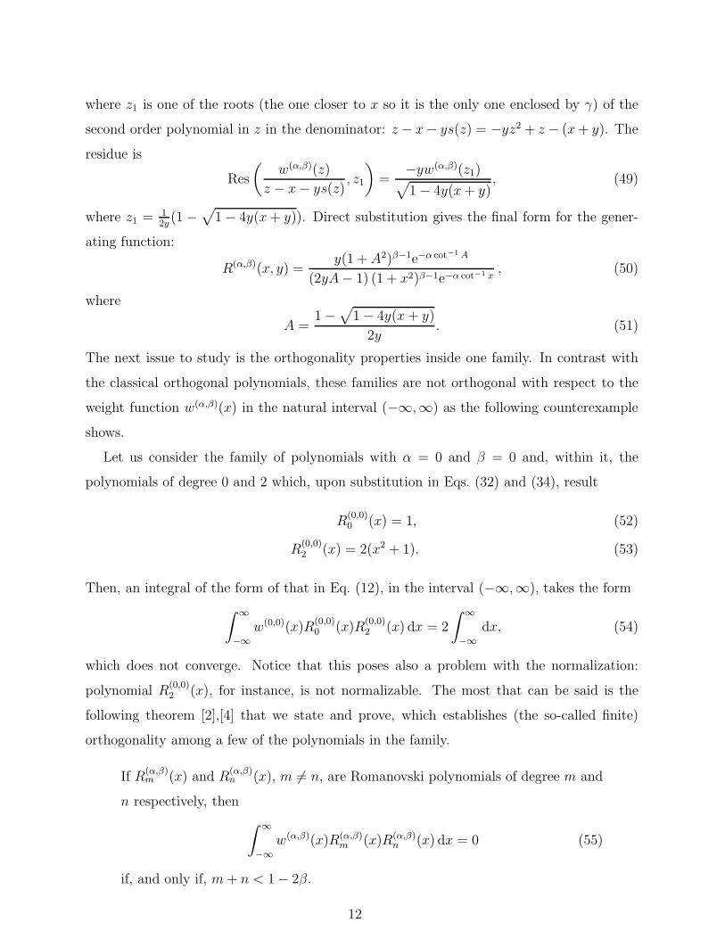
where z1 is one of the roots (the one closer to x so it is the only one enclosed by γ) of the

second order polynomial in z in the denominator: z − x− ys(z) = −yz2 + z − (x+ y). The

residue is

Res

(w(α,β)(z)

z − x− ys(z), z1

)=

−yw(α,β)(z1)√1− 4y(x+ y)

, (49)

where z1 = 12y(1 −

√1− 4y(x+ y)). Direct substitution gives the final form for the gener-

ating function:

R(α,β)(x, y) =y(1 + A2)β−1e−α cot−1 A

(2yA− 1) (1 + x2)β−1e−α cot−1 x, (50)

where

A =1−

√1− 4y(x+ y)

2y. (51)

The next issue to study is the orthogonality properties inside one family. In contrast with

the classical orthogonal polynomials, these families are not orthogonal with respect to the

weight function w(α,β)(x) in the natural interval (−∞,∞) as the following counterexample

shows.

Let us consider the family of polynomials with α = 0 and β = 0 and, within it, the

polynomials of degree 0 and 2 which, upon substitution in Eqs. (32) and (34), result

R(0,0)0 (x) = 1, (52)

R(0,0)2 (x) = 2(x2 + 1). (53)

Then, an integral of the form of that in Eq. (12), in the interval (−∞,∞), takes the form

∫ ∞

−∞

w(0,0)(x)R(0,0)0 (x)R

(0,0)2 (x) dx = 2

∫ ∞

−∞

dx, (54)

which does not converge. Notice that this poses also a problem with the normalization:

polynomial R(0,0)2 (x), for instance, is not normalizable. The most that can be said is the

following theorem [2],[4] that we state and prove, which establishes (the so-called finite)

orthogonality among a few of the polynomials in the family.

If R(α,β)m (x) and R

(α,β)n (x), m 6= n, are Romanovski polynomials of degree m and

n respectively, then

∫ ∞

−∞

w(α,β)(x)R(α,β)m (x)R(α,β)

n (x) dx = 0 (55)

if, and only if, m+ n < 1− 2β.

12

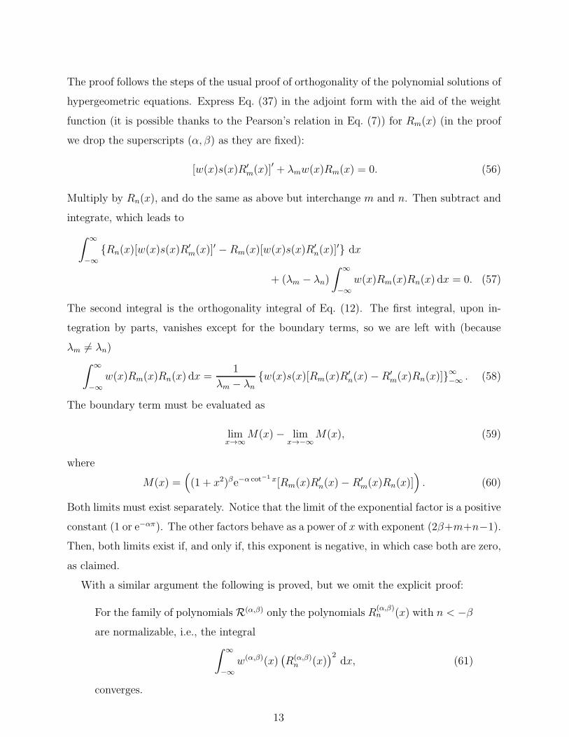
The proof follows the steps of the usual proof of orthogonality of the polynomial solutions of

hypergeometric equations. Express Eq. (37) in the adjoint form with the aid of the weight

function (it is possible thanks to the Pearson’s relation in Eq. (7)) for Rm(x) (in the proof

we drop the superscripts (α, β) as they are fixed):

[w(x)s(x)R′m(x)]

′+ λmw(x)Rm(x) = 0. (56)

Multiply by Rn(x), and do the same as above but interchange m and n. Then subtract and

integrate, which leads to

∫ ∞

−∞

{Rn(x)[w(x)s(x)R′m(x)]

′ − Rm(x)[w(x)s(x)R′n(x)]

′} dx

+ (λm − λn)

∫ ∞

−∞

w(x)Rm(x)Rn(x) dx = 0. (57)

The second integral is the orthogonality integral of Eq. (12). The first integral, upon in-

tegration by parts, vanishes except for the boundary terms, so we are left with (because

λm 6= λn)∫ ∞

−∞

w(x)Rm(x)Rn(x) dx =1

λm − λn{w(x)s(x)[Rm(x)R

′n(x)− R′

m(x)Rn(x)]}∞−∞ . (58)

The boundary term must be evaluated as

limx→∞

M(x)− limx→−∞

M(x), (59)

where

M(x) =((1 + x2)βe−α cot−1 x[Rm(x)R

′n(x)− R′

m(x)Rn(x)]). (60)

Both limits must exist separately. Notice that the limit of the exponential factor is a positive

constant (1 or e−απ). The other factors behave as a power of x with exponent (2β+m+n−1).

Then, both limits exist if, and only if, this exponent is negative, in which case both are zero,

as claimed.

With a similar argument the following is proved, but we omit the explicit proof:

For the family of polynomials R(α,β) only the polynomials R(α,β)n (x) with n < −β

are normalizable, i.e., the integral∫ ∞

−∞

w(α,β)(x)(R(α,β)

n (x))2

dx, (61)

converges.

13

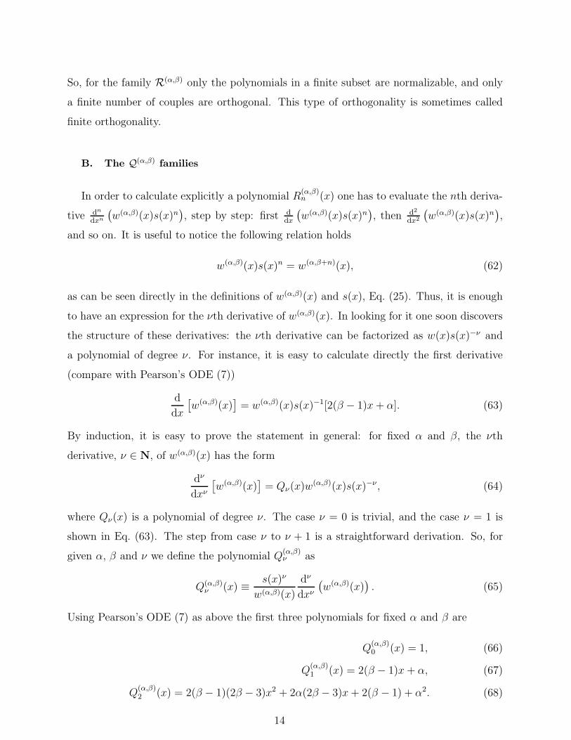
So, for the family R(α,β) only the polynomials in a finite subset are normalizable, and only

a finite number of couples are orthogonal. This type of orthogonality is sometimes called

finite orthogonality.

B. The Q(α,β) families

In order to calculate explicitly a polynomial R(α,β)n (x) one has to evaluate the nth deriva-

tive dn

dxn

(w(α,β)(x)s(x)n

), step by step: first d

dx

(w(α,β)(x)s(x)n

), then d2

dx2

(w(α,β)(x)s(x)n

),

and so on. It is useful to notice the following relation holds

w(α,β)(x)s(x)n = w(α,β+n)(x), (62)

as can be seen directly in the definitions of w(α,β)(x) and s(x), Eq. (25). Thus, it is enough

to have an expression for the νth derivative of w(α,β)(x). In looking for it one soon discovers

the structure of these derivatives: the νth derivative can be factorized as w(x)s(x)−ν and

a polynomial of degree ν. For instance, it is easy to calculate directly the first derivative

(compare with Pearson’s ODE (7))

d

dx

[w(α,β)(x)

]= w(α,β)(x)s(x)−1[2(β − 1)x+ α]. (63)

By induction, it is easy to prove the statement in general: for fixed α and β, the νth

derivative, ν ∈ N, of w(α,β)(x) has the form

dν

dxν[w(α,β)(x)

]= Qν(x)w

(α,β)(x)s(x)−ν , (64)

where Qν(x) is a polynomial of degree ν. The case ν = 0 is trivial, and the case ν = 1 is

shown in Eq. (63). The step from case ν to ν + 1 is a straightforward derivation. So, for

given α, β and ν we define the polynomial Q(α,β)ν as

Q(α,β)ν (x) ≡ s(x)ν

w(α,β)(x)

dν

dxν(w(α,β)(x)

). (65)

Using Pearson’s ODE (7) as above the first three polynomials for fixed α and β are

Q(α,β)0 (x) = 1, (66)

Q(α,β)1 (x) = 2(β − 1)x+ α, (67)

Q(α,β)2 (x) = 2(β − 1)(2β − 3)x2 + 2α(2β − 3)x+ 2(β − 1) + α2. (68)

14

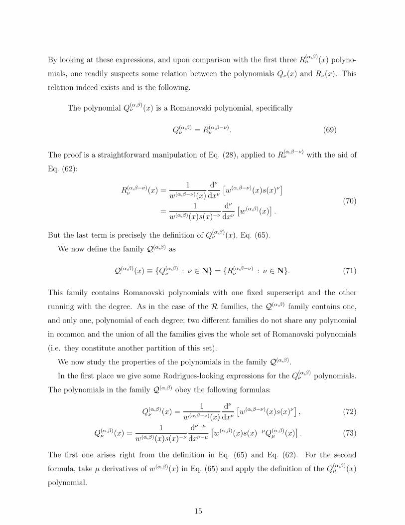
By looking at these expressions, and upon comparison with the first three R(α,β)n (x) polyno-

mials, one readily suspects some relation between the polynomials Qν(x) and Rν(x). This

relation indeed exists and is the following.

The polynomial Q(α,β)ν (x) is a Romanovski polynomial, specifically

Q(α,β)ν = R(α,β−ν)

ν . (69)

The proof is a straightforward manipulation of Eq. (28), applied to R(α,β−ν)ν with the aid of

Eq. (62):

R(α,β−ν)ν (x) =

1

w(α,β−ν)(x)

dν

dxν[w(α,β−ν)(x)s(x)ν

]

=1

w(α,β)(x)s(x)−ν

dν

dxν[w(α,β)(x)

].

(70)

But the last term is precisely the definition of Q(α,β)ν (x), Eq. (65).

We now define the family Q(α,β) as

Q(α,β)(x) ≡ {Q(α,β)ν : ν ∈ N} = {R(α,β−ν)

ν : ν ∈ N}. (71)

This family contains Romanovski polynomials with one fixed superscript and the other

running with the degree. As in the case of the R families, the Q(α,β) family contains one,

and only one, polynomial of each degree; two different families do not share any polynomial

in common and the union of all the families gives the whole set of Romanovski polynomials

(i.e. they constitute another partition of this set).

We now study the properties of the polynomials in the family Q(α,β).

In the first place we give some Rodrigues-looking expressions for the Q(α,β)ν polynomials.

The polynomials in the family Q(α,β) obey the following formulas:

Q(α,β)ν (x) =

1

w(α,β−ν)(x)

dν

dxν[w(α,β−ν)(x)s(x)ν

], (72)

Q(α,β)ν (x) =

1

w(α,β)(x)s(x)−ν

dν−µ

dxν−µ

[w(α,β)(x)s(x)−µQ(α,β)

µ (x)]. (73)

The first one arises right from the definition in Eq. (65) and Eq. (62). For the second

formula, take µ derivatives of w(α,β)(x) in Eq. (65) and apply the definition of the Q(α,β)µ (x)

polynomial.

15

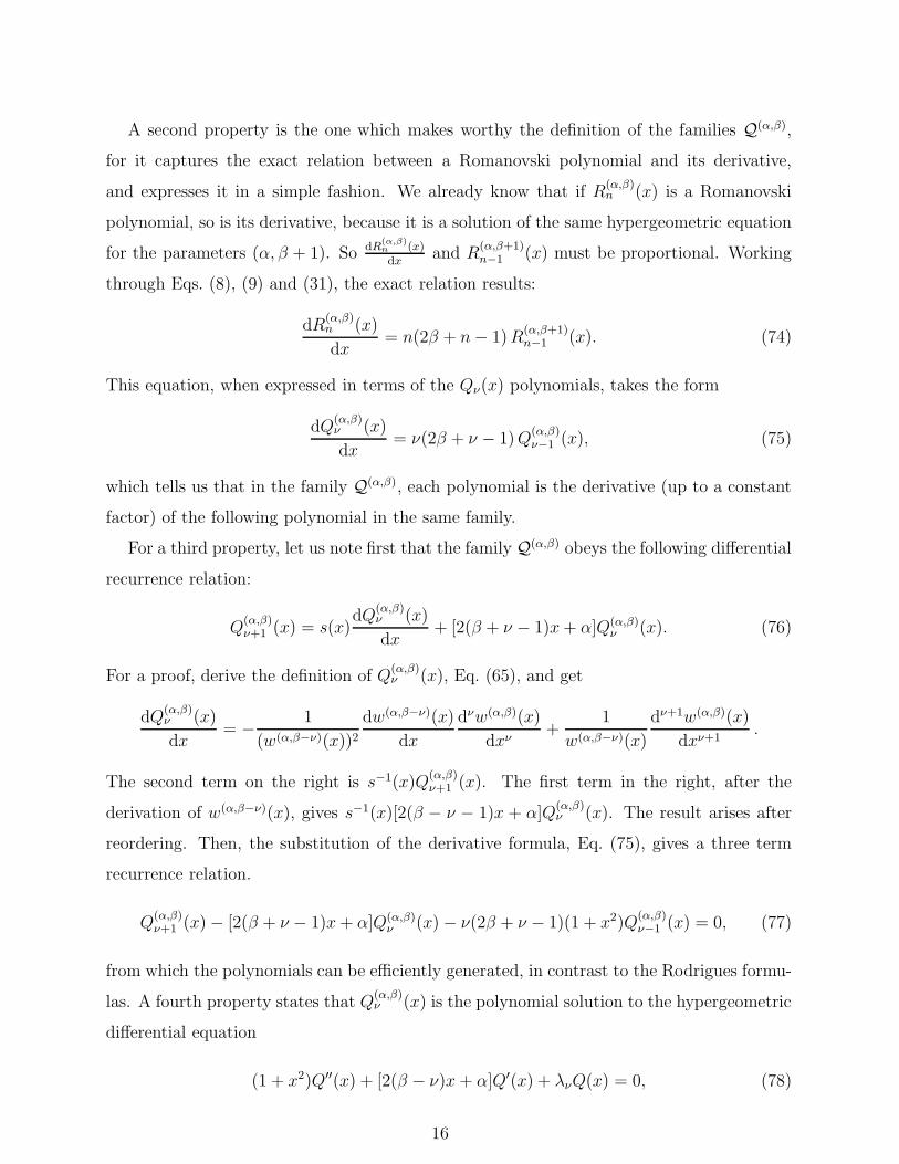
A second property is the one which makes worthy the definition of the families Q(α,β),

for it captures the exact relation between a Romanovski polynomial and its derivative,

and expresses it in a simple fashion. We already know that if R(α,β)n (x) is a Romanovski

polynomial, so is its derivative, because it is a solution of the same hypergeometric equation

for the parameters (α, β + 1). So dR(α,β)n (x)dx

and R(α,β+1)n−1 (x) must be proportional. Working

through Eqs. (8), (9) and (31), the exact relation results:

dR(α,β)n (x)

dx= n(2β + n− 1)R

(α,β+1)n−1 (x). (74)

This equation, when expressed in terms of the Qν(x) polynomials, takes the form

dQ(α,β)ν (x)

dx= ν(2β + ν − 1)Q

(α,β)ν−1 (x), (75)

which tells us that in the family Q(α,β), each polynomial is the derivative (up to a constant

factor) of the following polynomial in the same family.

For a third property, let us note first that the family Q(α,β) obeys the following differential

recurrence relation:

Q(α,β)ν+1 (x) = s(x)

dQ(α,β)ν (x)

dx+ [2(β + ν − 1)x+ α]Q(α,β)

ν (x). (76)

For a proof, derive the definition of Q(α,β)ν (x), Eq. (65), and get

dQ(α,β)ν (x)

dx= − 1

(w(α,β−ν)(x))2dw(α,β−ν)(x)

dx

dνw(α,β)(x)

dxν+

1

w(α,β−ν)(x)

dν+1w(α,β)(x)

dxν+1.

The second term on the right is s−1(x)Q(α,β)ν+1 (x). The first term in the right, after the

derivation of w(α,β−ν)(x), gives s−1(x)[2(β − ν − 1)x + α]Q(α,β)ν (x). The result arises after

reordering. Then, the substitution of the derivative formula, Eq. (75), gives a three term

recurrence relation.

Q(α,β)ν+1 (x)− [2(β + ν − 1)x+ α]Q(α,β)

ν (x)− ν(2β + ν − 1)(1 + x2)Q(α,β)ν−1 (x) = 0, (77)

from which the polynomials can be efficiently generated, in contrast to the Rodrigues formu-

las. A fourth property states that Q(α,β)ν (x) is the polynomial solution to the hypergeometric

differential equation

(1 + x2)Q′′(x) + [2(β − ν)x+ α]Q′(x) + λνQ(x) = 0, (78)

16

where λν = −ν(2β − ν − 1). This equation is just the hypergeometric differential equation

(37) for the polynomial R(α,β−ν)ν (x), which is Q

(α,β)ν (x), so it is proved.

The fifth property is that there exists a generating function Q(α,β)(x, y) in closed form

for the family Q(α,β), which is an analytic function whose Taylor expansion in the variable

y is given by

Q(α,β)(x, y) =∞∑

ν=0

yν

ν!Q(α,β)

ν (x). (79)

By substituting the definition of Q(α,β)ν (x), Eq. (65), in previous equation and grouping

factors and setting z = x+ ys(x) we get

Q(α,β)(x, y) =1

w(α,β)(x)

∞∑

ν=0

[ys(x)]ν

ν!

dν

dxν[w(α,β)(x)

]

=1

w(α,β)(x)

∞∑

ν=0

(z − x)ν

ν!

dν

dzν[w(α,β)(z)

]|z=x,

(80)

which is a Taylor expansion of the function inside the derivative at the point (x + ys(x))

with base point x. Thus, the summation of the series is given by w(α,β) at the point B =

x+ ys(x) = x+ y(1 + x2). The result is

Q(α,β)(x, y) =(1 +B2)β−1e−α cot−1 B

(1 + x2)β−1e−α cot−1 x, (81)

from which numerous recursion relations, such as Eq. (77), may be derived as usual [17],

[18], [19].

We now address an orthogonality property of the Q(α,β)ν (x) polynomials. Polynomials in

the family Q(α,β), with β < ε− 12, satisfy the following relation:

∫ ∞

−∞

w(α,β)(x)

s(x)ε2

Q(α,β)m (x)

s(x)m2

Q(α,β)n (x)

s(x)n2

dx = 0, (82)

where m 6= n and ε = 1 if m+n is odd, and ε = 2 if m+n is even. This is an orthogonality

integral between the functions Q(α,β)m /s(x)m/2 and Q

(α,β)n /s(x)n/2 built on top of the poly-

nomials in Q(α,β). In contrast to the orthogonality relations in the R(α,β) families, which

are valid only for a finite subfamily of polynomials, Eq. (82) applies to the whole family

Q(α,β). In terms of the Romanovski polynomials in Eq. (69) the integral in Eq. (82) takes

the following form

∫ ∞

−∞

√w(α,β−m)(x)R(α,β−m)

m (x)√w(α,β−n)(x)R(α,β−n)

n (x)1

s(x)ε2

dx = 0, (83)

17

which can be read as orthogonality within the infinite sequence of polynomials R(α,β−k)k with

a running parameter attached to the polynomial degree.

In fact, Eq. (82) stands for two different results which require separate proofs. In any

case, since m 6= n, we can take m > n. Let us consider first the case of even m+ n. Then,

the integral of Eq. (82) is

Om,n =

∫ ∞

−∞

w(α,β)(x)

s(x)

Q(α,β)m (x)

s(x)m2

Q(α,β)n (x)

s(x)n2

dx. (84)

Upon substitution of Q(α,β)m (x) by its definition, Eq. (65), we get

Om,n =

∫ ∞

−∞

s(x)12(m−n)−1Q(α,β)

n (x)dm

dxmw(α,β)(x) dx. (85)

Because m + n is even and m > n, then m− n− 2 is an even, nonnegative, integer. Thus,

s(x)12(m−n)−1 is a polynomial of degree m−n−2 and s(x)

12(m−n)−1Q

(α,β)n (x) is a polynomial of

degree m−2, which we call Pm−2. Then, after m−1 integrations by parts, m−1 derivatives

are applied to Pm−2 so it vanishes and we are left only with the boundary terms.

Om,n =

m−1∑

k=1

(−1)k−1

[dk−1Pm−2(x)

dxk−1

dm−kw(α,β)(x)

dxm−k

]∞

−∞

. (86)

For each k, the derivative of Pm−2 is a polynomial of degree m − k − 1 whereas the m− k

derivative of w(α,β) is given in terms of the polynomial Q(α,β)m−k , again by its definition in

Eq. (65). Then, the k boundary term results

dk−1Pm−2(x)

dxk−1

dm−kw(α,β)(x)

dxm−k= e−α cot−1 x(1 + x2)β−m+k−1P2m−2k−1(x), (87)

where P2m−2k−1 is a polynomial of degree 2m − 2k − 1. The asymptotic behavior of this

term at ±∞ is the same as x2β−3 and, thus, it goes to zero if, and only if, β < 32.

The proof of the case with (m+ n) odd is similar.

IV. RELATIONSHIP BETWEEN ROMANOVSKI POLYNOMIALS AND JA-

COBI POLYNOMIALS

Romanovski and Jacobi polynomials are closely related. In fact, it is common that

Romanovski polynomials are referred to as complexified Jacobi polynomials [1], [10]. In

this section we are showing which is the precise relationship between them and which is not:

18

Romanovski polynomials can indeed be obtained from a generalization of Jacobi polynomials

to the complex plane, but not through the complexification of Jacobi polynomials, which is

a different issue. Let us distinguish both concepts.

For ease of reference, we recall here equations (1) and (2), which are the equations

Romanovski polynomials and Jacobi polynomials solve, respectively.

(1 + x2)R′′ + t(x)R′ + λR = 0, (88a)

(1− x2)P ′′ + t(x)P ′ + λP = 0, (88b)

where t(x) is a polynomial of, at most, first degree.

The argument of the complexification is based on the fact that the change from x to ix

transforms the coefficient (1−x2) in Eq. (88b) into (1+x2), the coefficient in Eq. (88a). But

caution is needed with this idea. Complexification is a transformation which takes real valued

functions of a real variable into complex functions of a real variable. If g : U ⊂ R → R is

such a real valued function, defined in an open subset of the real line, we define the function

g : U ′ ⊂ U → C by the recipe (wherever it makes sense)

g(x) ≡ g(ix). (89)

The new function g may, or may not, be well defined in all the points of U and may, or may

not, inherit the continuity and differentiability properties of g in all points of U (think, for

an instance, of the function g(x) = (1 + x2)−1). In the case g happens to be a polynomial

it is easy to see that both continuity and differentiability are indeed respected. Then, the

derivatives of g and g with respect to x satisfy the following identity:

g(n) = ing(n),

n ∈ {0, 1, . . . }.(90)

Complexification respects the sum and product operations, i.e., ˜f + g = f + g and f g = f g

(it is a ring homomorphism from a ring of real valued functions of a real variable to the

ring of complex valued functions of a real variable). Thus, if the function g is a solution

to a linear differential equation, then g is a solution of the complexification of that linear

differential equation. The application of this argument to the Jacobi polynomials gives the

result that P(α,β)n (x) ≡ P

(α,β)n (ix) verifies the complexification of Eq. (88b), namely

(1 + x2)(P )′′ + i t(ix)(P )′ − λP = 0, (91)

19

where the prime still stands for derivative with respect to the real variable x. But equation

(91) is not the same as equation (88a) unless i t(ix) is real. If we write t(x) = β − α− (α+

β + 2)x, as is customary in the Jacobi equation (see Eq. (19)), we need (α + β + 2) to be

real and (β−α) to be imaginary, which is achieved only if α and β are complex and β = α∗.

Hence we have to consider the functions P(α,β)n (ix) with complex parameters α and β which

are no longer the complexification of the classical Jacobi polynomials as described above. So,

the complexification of Jacobi polynomials does not result in the Romanovski polynomials.

But, even in case it did, not all the properties of Jacobi polynomials would be translated to

properties of Romanovski polynomials: only those which made use of theorems like equation

(90), which relates the derivatives. For instance, there is no theorem relating integrals of

a complexified function and the original function; thus, all the properties depending on

integrations, such as the orthogonality, would have no translation to the complexified version.

An alternative scenario is to extend the definition of Jacobi polynomials to the complex

plane: complex variable z, complex parameters α and β and, obviously, complex values. In

[20] this definition has been successfully given as

P (α,β)n (z) ≡ 1

2n

n∑

k=0

(n+ α

n− k

)(n+ β

k

)(1− z)k(1 + z)n−k (92)

or, equivalently, by the Rodrigues formula

P (α,β)n (z) =

1

2nn!(1− z)−α(1 + z)−β d

n

dzn[(1− z)n+α(1 + z)n+β

], (93)

which are formally the same as the classical ones except now z, α, β ∈ C while n ∈{0, 1, 2, . . .}. These polynomials solve the complex Jacobi ODE

(1− z2)P ′′(z) + [β − α− (α+ β + 2)z]P ′(z) + (α + β + 1 + n)nP (z) = 0, (94)

where the prime stands now for the derivative with respect to the complex variable z.

The specialization of the variable to the imaginary axis, z = ix, and the parameters to

β = α∗ leaves us with Eq. (88a) (notice the change from d/dz to d/dx gives an extra i), so

these complex Jacobi polynomials solve the differential equation that define the Romanovski

polynomials. One has to prove now that functions P(α,α∗)n (z) restricted to z = ix are real

valued or, at least, proportional to a real valued one. This is easily achieved by computing

the complex conjugate of the function P(α,α∗)n (ix) in terms of the definition in Eq. (92)

P (α,α∗)n (ix)∗ =

(−1)n

2n

n∑

k=0

(n+ α∗

n− k

)(n+ α

k

)(1 + ix)k(1− ix)n−k. (95)

20

With a change in the summation index from k to l = n− k, we get

P (α,α∗)n (ix)∗ = (−1)nP (α,α∗)

n (ix), (96)

i.e., for even n, P(α,α∗)n (ix) is real, while for odd n, it is imaginary. Hence, the combination

inP(α,α∗)n (ix) is a real function for all n. Finally, because the polynomial solutions of a

hypergeometric differential equation are unique for each degree, up to a constant factor,

we conclude that inP(α,α∗)n (ix) is the Romanovski polynomial of degree n with parameters

−2ℑ(α) and −(ℜ(α) + 1). In other words, complex Jacobi polynomials do provide another

characterization of the Romanovski polynomials via

R(α,β)n (x) = inP

(1−β− i2α,1−β+ i

2α)

n (ix), (97)

(with suitably chosen normalization constants for the Jacobi polynomials). However, this

alternative characterization is of no help when it comes to study the orthogonality properties,

because the orthogonality properties of the complex Jacobi polynomials are not well known.

In [20] the authors state some new results on the orthogonality along some particular paths

in the complex plane. For instance, in their Eq. (4.3) an orthogonality relation is given

along the imaginary axis, which is our case, but only for a special case demanding real, not

integer, parameters, which is not our case. To our knowledge, at the present time there are

no results concerning the orthogonality of these complex polynomials which would provide

an alternative approach to the results on orthogonality stated in Subsection IIIA.

The argument presented here states that Romanovski polynomials are just a subset of

complex Jacobi polynomials. Therefore it may seem that Romanovski polynomials are,

somehow, subordinated to the Jacobi polynomials. But the whole argument could be re-

versed if we had a definition of complex Romanovski polynomials as the one given in Ref. [20]

(here reproduced in Eq. (92)). If that would be the case, it would not be surprising to get

a relation of the form

P (α,β)n (x) = −(in)R

(i(α−β), 12(α+β)+1)

n (ix),

where, now, P(α,β)n (x) is a real Jacobi polynomial and R

(i(α−β), 12(α+β)+1)

n (ix) would be a

complex Romanovski polynomial. But, as we do not have such a definition, this last formula

is nothing but a conjecture.

21

V. ROMANOVSKI POLYNOMIALS IN SELECTED QUANTUM MECHANICS

PROBLEMS

The Romanovski polynomials are part of the exact solutions of several problems in ordi-

nary and supersymmetric quantum mechanics. In this section we review a few prominent

cases. The selection of the examples certainly reflects personal preferences and does not

pretend to be complete.

In general, the exactly soluble Schrodinger equations enjoy a special status because most

of them describe phenomena that play a key role in physics. Suffice it to mention in that

regard such textbook examples as the description of the spectrum of the hydrogen atom in

terms of the Coulomb potential [21], or the description of vibrational modes in molecules and

nuclei in terms of the Hulthen and Morse potentials [22], [23]. More recently, exactly soluble

potentials acquired importance within the context of supersymmetric quantum mechanics

(SUSYQM) which considers the special class of Schrodinger equations (H(z)−E)Ψ(z) = 0,

with H(z) standing for the Hamiltonian (of the one-dimensional, real variable z), and E

for the energy, which allow [24] a factorization of H(z) according to H(z) = A+(z)A−(z) +

Egst, and A−(z)Ψgst(z) = 0. SUSYQM provides a powerful technique for finding the exact

solutions of Schrodinger equations. To be specific, any excited state can be obtained by

the successive action on the ground state, Ψgst(z), of an appropriate number of creation

operators, A+(z), defined in terms of the so-called superpotential, U(z), as

A±(z) ≡(± h√

2µ

d

dz+ U(z)

).

Supersymmetric quantum mechanics governs a family of exactly soluble potentials (see

Refs. [25]– [28] for details) two of which are the so-called hyperbolic Scarf and trigono-

metric Rosen-Morse potentials, that have been solved recently in [6], [7], [16] in terms of the

Romanovski polynomials as discussed in the next two subsections. The third subsection is

devoted to applications of the Romanovski polynomials in random matrix theory.

22

A. Romanovski polynomials in problems with non-central electric potentials

The (one-dimensional) Schrodinger equation with the hyperbolic Scarf potential is

(− h2

2µ

d2

dz2+ Vh(z)− E

)Ψ(z) = 0 ,

Vh(z) ≡ [B2 − A(A+ 1)]1

cosh2 z−B(2A+ 1) tanh z

1

cosh z.

(98)

This equation appears, among others, in the problem of a particle within a non-central scalar

potential, a result due to Ref. [9]. In denoting such a potential by V (r, θ), one can make for

it the specific choice of

V (r, θ) = V1(r) +V2(θ)

r2,

V2(θ) = −b cot θ.(99)

An interesting phenomenon is the electrostatic non-central potential in which case V1(r) is

the Coulomb potential. The corresponding Schrodinger equation

[− h2

2µ

[1

r2∂

∂rr2∂

∂r+

1

r2 sin θ

∂

∂θsin θ

∂

∂θ+

1

r2 sin2 θ

∂2

∂φ2

]+ V (r, θ)

]Ψ(r, θ, ϕ)

= EΨ(r, θ, ϕ) , (100)

is solved in the standard way by separating variables. As long as the potential does not

depend on the azimuthal angle, one assumes

Ψ(r, θ, φ) = R(r)Θ(θ)eimφ . (101)

The radial and angular differential equations for R(r) and Θ(θ) are then found as

d2R(r)

dr2+

2

r

dR(r)

dr+

[2µ

h2[V1(r) + E]− l(l + 1)

r2)

]R(r) = 0, (102)

andd2Θ(θ)

dθ2+ cot(θ)

dΘ(θ)

dθ+

[l(l + 1)− 2µV2(θ)

h2− m2

sin2 θ

]Θ(θ) = 0 , (103)

with l(l + 1) being the separation constant. From now on we will focus on the second

equation. Notice that for V2(θ) = 0, and upon changing variables from θ to cos θ, the last

equation transforms into the associated Legendre equation and correspondingly

Θ(θ)V2(θ)→0−−−−−→ Pm

l (cos θ) , (104)

23

an observation that will become important below.

Following Ref. [9] one begins with substituting the polar angle variable by a new variable,

z, introduced via θ = f(z), with f to be determined. This leads to the new equation

[d2

dz2+

[−f

′′(z)

f ′(z)+ f ′(z) cot f(z)

]d

dz

+

[−2µ

h2V2(f(z)) + l(l + 1)− m2

sin2 f(z)

]f ′ 2(z)

]ψ(z) = 0 (105)

with f ′(z) ≡ df(z)dz

, and ψ(z) defined as ψ(z) ≡ Θ(f(z)). Next one can require that f ′(z)

approaches zero at z = 0 like sin z, meaning, limz→0 f′(z)/ sin z = 1, and define f(z) via

f ′′(z)

f ′(z)= f ′(z) cot f(z) . (106)

The latter equation is solved by f(z) = 2 tan−1 ez. With this relation one finds that

sin θ =1

cosh z, cos θ = − tanh z , (107)

and consequently, f ′(z) = sin f(z) = sech z. Upon substituting the last relations into

Eqs. (99), and (105), one arrives at

d2ψ(z)

dz2+

[l(l + 1)

1

cosh2 z− 2µ

h2b tanh z

1

cosh z−m2

]ψ(z) = 0 . (108)

In taking in consideration Eqs. (98), (107) one realizes that the letter equation is precisely

the one-dimensional Schrodinger equation with the hyperbolic Scarf potential and with

• l(l + 1) playing the role of −(B2 − A(A+ 1))/(h2/(2µ)

),

• m2 playing the role of −En/(h2/(2µ)

),

• b playing the role of −B(2A + 1).

This equation has been solved in terms of the Romanovski polynomials in Ref. [6] upon sub-

stituting sinh z = x. Notice that there the weight function was defined as (1+x2)−peq tan−1 x,

and the polynomials have been labeled correspondingly as R(p,q)n (x), following [29]. A com-

parison with Eq. (25) allows identifying p −→ −β + 1, q −→ α. In terms of the notations

of the present work, the result of Ref. [6] can be cast into the following form:

ψn(z) = Cn[1 + (sinh z)2]β

2− 1

4 eα2tan−1 sinh zR(α,β)

n (sinh z),

α = −2B, β = −A +1

2, En = −(A− n)2 ,

(109)

24

with Cn being a normalization constant. Back to the θ variable and in making use of the

equality xdef:= sinh z = − cot θ, we find

Θ(θ) = ψn(sinh1(− cot θ)) = Cn[1 + (cot θ)2]

β2− 1

4 eα2tan−1(− cot θ)R(α,β)

n (− cot θ), (110)

showing that the angular part of the exact solution to the non-central potential under con-

sideration is defined by the Romanovski polynomials. In turning off the non-central piece

of the potential, the angular part of the solutions will become the standard spherical har-

monics, Y ml (θ, φ) = Pm

l (θ) eimφ, which will produce a relationship between the Romanovski

polynomials and the associated Legendre functions, an issue to be considered in more detail

at the end of this section.

Now, in accord with the theorem on the finite orthogonality of the Romanovski polyno-

mials in Eq. (55), also only a finite number of eigen-wave functions to the hyperbolic Scarf

potential appears orthogonal,∫ +∞

−∞

ψn(z)ψm(z)dz = CmCn

∫ +∞

∞

w(α,β)(x)R(α,β)m (x)R(α,β)

n (x) = δmn,

m+ n ≤ 2A .

(111)

This finite orthogonality reflects the finite number of bound states within the potential under

consideration.

Next, it is quite instructive to consider the case of a vanishing V2(θ), i.e. b = 0, and

compare Eq. (108) to Eq. (98) for B = 0. From now on we will give all quantities in units

of h = 1 = 2µ. In this case

• Eq. (108) reduces to the equation for the associated Legendre polynomials, Pml (cos θ),

• l becomes A,

• m2 becomes (l − n)2,

• Eq. (98) produces R(α=0,β=−l+ 1

2)

n (x) as part of its solutions,

which allows one to relate n to l and m as m = l − n. In taking into account Eq. (104)

together with cot θ = − sinh z provides the following relationship between the associated

Legendre functions and the Romanovski polynomials

Pml (cos θ) = const[1 + (cot θ)2]−

l2R

(0, 12−l)

m+l (− cot θ) ,

m+ l = n ∈ {0, 1, . . . , l}.(112)

25

In substituting the latter equation into the orthogonality integral between the associated

Legendre functions,

∫ 1

−1

Pml (cos θ)Pm

l′ (cos θ) d cos θ = 0,

l 6= l′,

(113)

we find∫ 1

−1

(1 + (cot θ)2)−l+l′

2 R(0, 1

2−l)

l+m (− cot θ)R(0, 1

2−l′)

l′+m (− cot θ)d cos θ = 0,

l 6= l′.

(114)

The latter relationship amounts to the following orthogonality integral

∫ ∞

−∞

(1 + (sinh z)2)−l+l′

2 R(0, 1

2−l)

n (sinh z)R(0, 1

2−l′)

n′ (sinh z)(sech z)2dz =

∫ ∞

−∞

√w(0, 1

2−l)(x)R

(0, 12−l)

n (x)

√w(0, 1

2−l′)(x)R

(0, 12−l′)

n′ (x)1

s(x)dx = 0,

x = sinh z, l − n = l′ − n′ = m ≥ 0, l 6= l′. (115)

Careful inspection shows that this equation is nothing but a particular case of the orthogo-

nality relation in the family of polynomials Q(α,β), established in Eq. (82) and translated to

the R(α,β)n notation in Eq. (83).

A further example is given by the Klein-Gordon equation with equal scalar and vector

potentials. It has been shown in Ref. [8] that the former can be reduced to the corresponding

Schrodinger equation. Therefore, in case one uses the hyperbolic Scarf potential in the above

Klein-Gordon equation, one will face again the Romanovski polynomials as part of its exact

solutions.

B. Romanovski polynomials in quark physics.

The interaction of quarks, the fundamental constituents of the baryons, are governed by

Quantum Chromodynamics (QCD) which is a non-Abelian gauge theory with gauge bosons

being the so called gluons. QCD predicts that the quark interactions run from one- to many

gluon exchanges over gluon self-interactions, the latter being responsible for the so-called

quark confinement, where highly energetic quarks remain trapped but behave as (asymptot-

ically) free particles at high energies and momenta. The QCD equations are nonlinear and

26

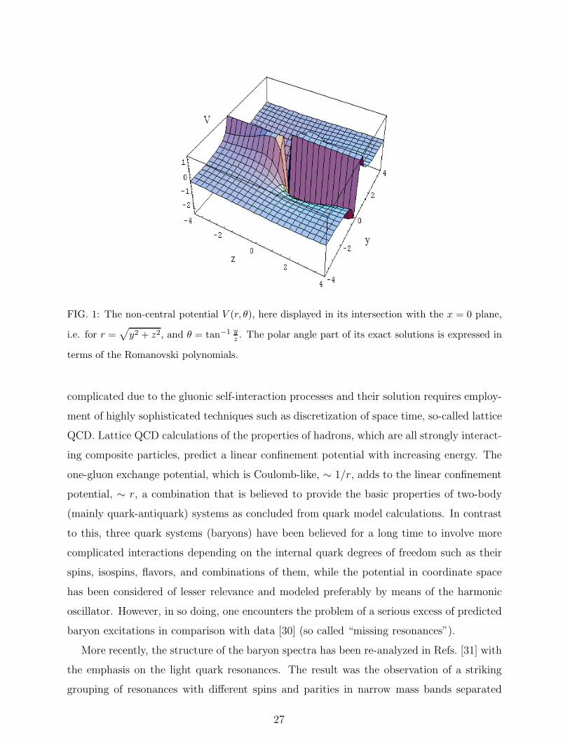
FIG. 1: The non-central potential V (r, θ), here displayed in its intersection with the x = 0 plane,

i.e. for r =√

y2 + z2, and θ = tan−1 yz . The polar angle part of its exact solutions is expressed in

terms of the Romanovski polynomials.

complicated due to the gluonic self-interaction processes and their solution requires employ-

ment of highly sophisticated techniques such as discretization of space time, so-called lattice

QCD. Lattice QCD calculations of the properties of hadrons, which are all strongly interact-

ing composite particles, predict a linear confinement potential with increasing energy. The

one-gluon exchange potential, which is Coulomb-like, ∼ 1/r, adds to the linear confinement

potential, ∼ r, a combination that is believed to provide the basic properties of two-body

(mainly quark-antiquark) systems as concluded from quark model calculations. In contrast

to this, three quark systems (baryons) have been believed for a long time to involve more

complicated interactions depending on the internal quark degrees of freedom such as their

spins, isospins, flavors, and combinations of them, while the potential in coordinate space

has been considered of lesser relevance and modeled preferably by means of the harmonic

oscillator. However, in so doing, one encounters the problem of a serious excess of predicted

baryon excitations in comparison with data [30] (so called “missing resonances”).

More recently, the structure of the baryon spectra has been re-analyzed in Refs. [31] with

the emphasis on the light quark resonances. The result was the observation of a striking

grouping of resonances with different spins and parities in narrow mass bands separated

27

by significant spacings. More specifically, it was found that to a very good accuracy, the

nucleon excitation levels carry the same degeneracies as the levels of the electron with spin

in the hydrogen atom, though the splittings of the former are quite different from those of

the latter. Namely, compared to the hydrogen atom, the baryon level splittings contain, in

addition to the Balmer term, also its inverse but of opposite sign. The same was found to

be valid for the excitation spectrum of the so called ∆(1232) particle, the most important

baryon excitation after the nucleon. The appeal of these results lies in the fact that no

state drops out of the systematics, on the one side, and that the number of “missing”

states predicted by it is significantly less than within all preceding schemes. The observed

degeneracies in the spectra of the light quark baryons have been attributed in Ref. [32] to

the dominance of a quark–antiquark configuration in baryon structure. Within the light of

these findings, the form of the potential in configuration space acquires importance anew.

In Refs. [7],[16] the case was made that the trigonometric Rosen-Morse potential provides

precisely degeneracies and level splittings as required by the light quark baryon spectra. The

trigonometric Rosen-Morse potential in the parametrization of Ref. [16] reads:

vtRM (z) = −2b cot z + l(l + 1)1

sin2 z, (116)

with l standing for the relative angular momentum between the quark and the di-quark in

units, as usual, of h = 1 = 2µ, and z = rdis a dimensionless variable built with a suited

length scale d.

The reason for the success of this potential in quark physics is that it captures the essential

traits of the QCD quark-gluon dynamics in interpolating between the Coulomb potential

(associated with the one-gluon exchange) and the infinite wall potential (associated with the

trapped but asymptotically free quarks) while passing through a linear confinement region

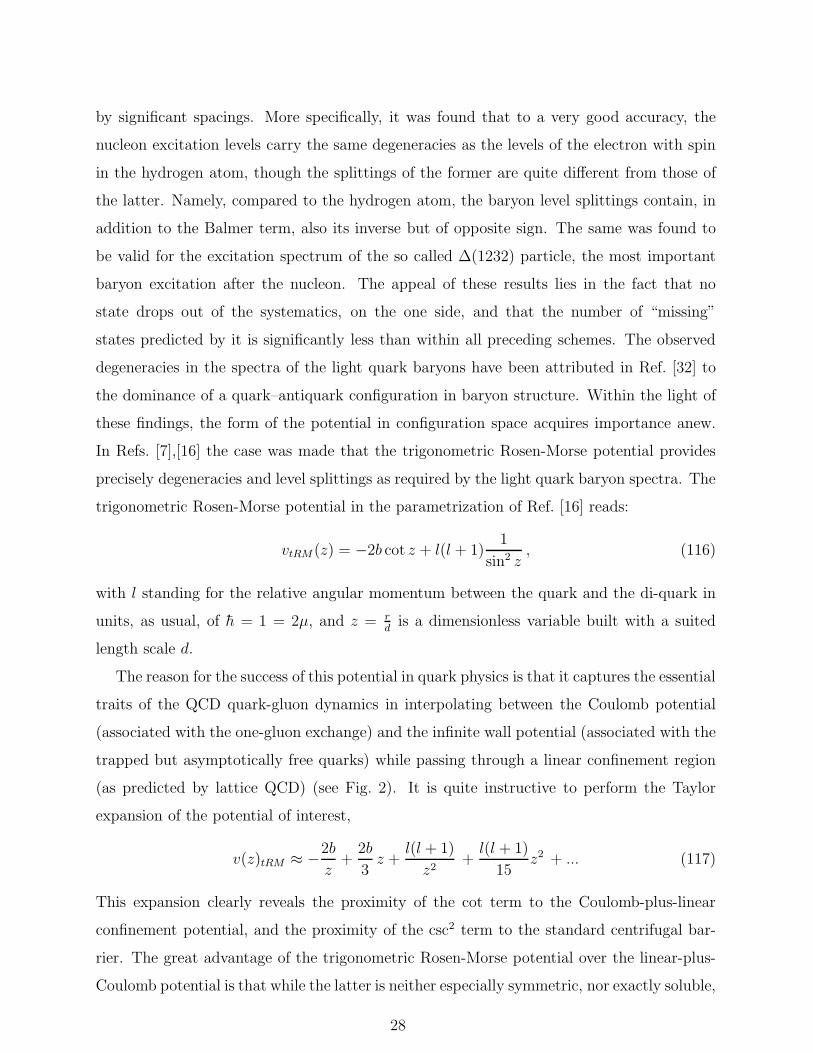
(as predicted by lattice QCD) (see Fig. 2). It is quite instructive to perform the Taylor

expansion of the potential of interest,

v(z)tRM ≈ −2b

z+

2b

3z +

l(l + 1)

z2+l(l + 1)

15z2 + ... (117)

This expansion clearly reveals the proximity of the cot term to the Coulomb-plus-linear

confinement potential, and the proximity of the csc2 term to the standard centrifugal bar-

rier. The great advantage of the trigonometric Rosen-Morse potential over the linear-plus-

Coulomb potential is that while the latter is neither especially symmetric, nor exactly soluble,

28

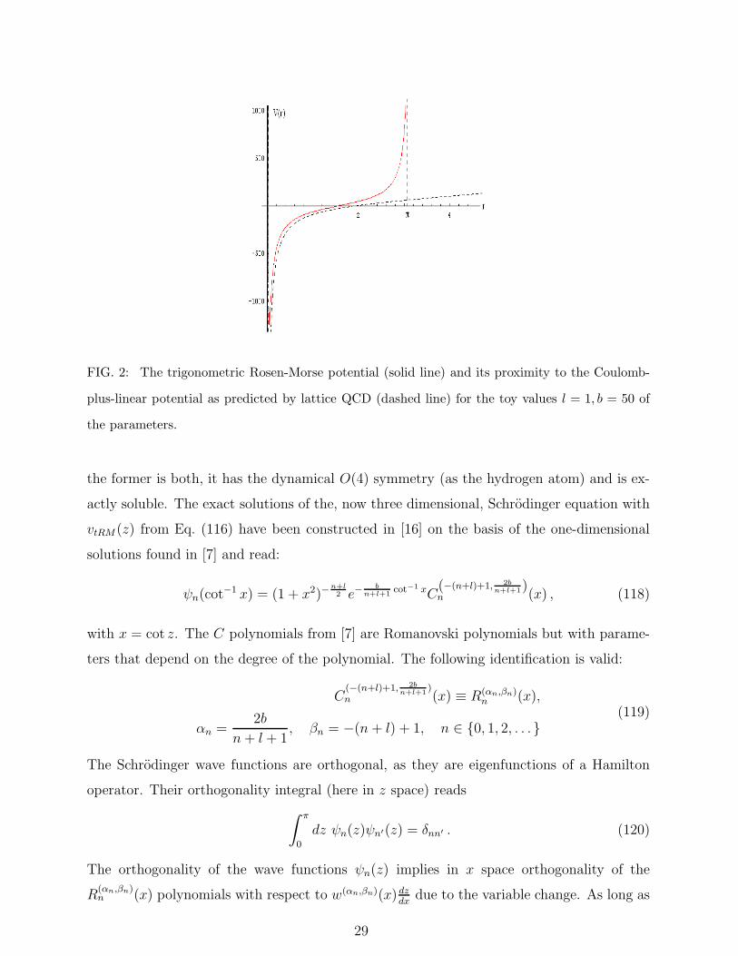
FIG. 2: The trigonometric Rosen-Morse potential (solid line) and its proximity to the Coulomb-

plus-linear potential as predicted by lattice QCD (dashed line) for the toy values l = 1, b = 50 of

the parameters.

the former is both, it has the dynamical O(4) symmetry (as the hydrogen atom) and is ex-

actly soluble. The exact solutions of the, now three dimensional, Schrodinger equation with

vtRM (z) from Eq. (116) have been constructed in [16] on the basis of the one-dimensional

solutions found in [7] and read:

ψn(cot−1 x) = (1 + x2)−

n+l2 e−

bn+l+1

cot−1 xC(−(n+l)+1, 2b

n+l+1)n (x) , (118)

with x = cot z. The C polynomials from [7] are Romanovski polynomials but with parame-

ters that depend on the degree of the polynomial. The following identification is valid:

C(−(n+l)+1, 2b

n+l+1)

n (x) ≡ R(αn,βn)n (x),

αn =2b

n+ l + 1, βn = −(n+ l) + 1, n ∈ {0, 1, 2, . . .}

(119)

The Schrodinger wave functions are orthogonal, as they are eigenfunctions of a Hamilton

operator. Their orthogonality integral (here in z space) reads

∫ π

0

dz ψn(z)ψn′(z) = δnn′ . (120)

The orthogonality of the wave functions ψn(z) implies in x space orthogonality of the

R(αn,βn)n (x) polynomials with respect to w(αn,βn)(x) dz

dxdue to the variable change. As long as

29

d cot−1 xdx

= −1/(1 + x2) = −1/s(x) then the orthogonality integral takes the form

∫ ∞

−∞

dx

s(x)

√w(αn,βn)(x)R(αn,βn)

n (x)√w(αn′ ,βn′)(x)R

(αn′ ,βn′)n′ (x) = δnn′ . (121)

To recapitulate, the Romanovski polynomials have been shown to be important ingredients

of the wave functions of quarks in accord with QCD quark-gluon dynamics.

C. Romanovski polynomials in random matrix theory

Random matrix theory was pioneered by Wigner [33] for the sake of modeling spectra

of heavy nuclei which are characterized by complicated interactions between large numbers

of protons and neutrons. Wigner’s idea was to limit the infinite dimensional Hamiltonian

matrix in configuration space to a finite, real quadratic (N × N), and symmetric, matrix

with elements being chosen at random from a suitable probability density distribution, say,

the Gaussian one. Along this line one can then model the densities of the nuclear states

as averages over the weighted sets of matrices. The advantage of this method is that as

N −→ ∞, the (normalized) eigenvalues of any randomly chosen matrix approach the limits

of the corresponding system averages, much like the general limit theorem. The probability

density distribution (p.d.f.) of the eigenvalues of the Gaussian ensemble of random matrices

is given by (the presentation in this section closely follows Ref. [34]):

1

CNe−

12

PNj=1 λ

2j

∏

1≤j<k≤N

|λk − λj |, (122)

where CN is the normalization constant and λi are the eigenvalues. Besides the Gaussian

random ensemble there are other random matrix ensembles under consideration in quantum

physics such as the circular Jacobi ensemble and the Cauchy ensemble, and precisely these

are of interest in the present section. However, their definitions require us to go beyond

the ensembles of random real matrices and consider matrices with complex entries. To be

more specific, one considers random ensembles composed by symmetric, unitary matrices, in

which case the theory is not developed from an explicit distribution density function for their

elements but rather from the requirement of the existence of a certain appropriate uniform

measure. The random unitary matrix ensemble is special not only because it forms a group

but mainly because this group is compact and allows for the definition of the so called Haar

volume, which then provides the uniform measure on the space as required above.

30

Definition: The circular unitary ensemble is the group of unitary matrices U

endowed with the volume form (dHU) = 1C

(U†U

)= idM2 with M2 hermitian.

The eigenvalues of the circular ensembles are confined to the unit circle, i.e. to λj = eiθj

with −π < θj < π. The associated probability density distribution of the eigenvalues is then

given by

1

C

∏

1≤j<k≤N

|eiθk − eiθj | ,

−π < θl < π .

(123)

More generally, an ensemble of unitary and symmetric matrices has an eigenvalues p.d.f of

the form (in the notations of Ref. [34])

N∏

l=1

w2(zl)∏

1≤j≤k≤N

|zk − zj |,

z = eiθ = e2πixL , θ ∈ [0, 2π), x ∈ [0, L) ,

(124)

where w2(zl) is a specific weight function. The circular Jacobi ensemble is specified by

w2(z) = |1− z|2a . (125)

A relevant research goal in quantum physics is finding the spacings in the spectra of the

circular Jacobi ensemble. Compared to the state densities, the calculation of gap proba-

bilities in the spectra deserves special efforts. In this section we review briefly the concept

for the calculation of gap probabilities in the circular Jacobi ensemble by means of the so

called Cauchy random matrix ensemble, a venue that will conduct us one more time to the

Romanovski polynomials .

To begin with, one considers the mapping

eiθ =1 + iλ

1− iλ, (126)

which maps each point λ on the real line to a point θ on the unit circle (measured anticlock-

wise from the origin) via a stereographic projection. Changing correspondingly variables in

Eqs. (124)–(125) amounts to the following eigenvalue p.d.f.:

N∏

l=1

(1 + λ2j)−N−a

∏

1≤j≤k≤N

|λk − λj| ,

λj ∈ (−∞,+∞) .

(127)

31

As long as one recognizes in the weight function the Cauchy weight, the random unitary

matrix ensemble generated this way is termed the Cauchy ensemble. On the other hand,

a comparison with the weight function of the Romanovski polynomials reveals the Cauchy

weight as w(0,−N−a+1)(x), an observation that will acquire a profound importance in the

following.

Back to the main goal, the gap probability, or better, the probability for no eigenvalues

in a region I, denoted by E(0, I), and for the case of any ensemble is now calculated as [34]

E(0, I) = 1 +∞∑

n=1

(−1)n

n!

∫

I

dx1...

∫

I

dxndetN−1∑

l=0

√w2(xi)pl(xi)

√w2(xj)pl(xj) , (128)

where pl(x) with l = 0, 1, 2, ... stand for the orthogonal polynomials associated with the

weight function w2(x). In other words, knowing the orthogonal polynomials is crucial for

the calculation of gap probabilities in any random matrix ensemble. In the specific case under

consideration, one seems to have two options in the choice for those polynomials, Romanovski

versus Jacobi polynomials in accord with their relationship established in Eq. (97). The

choice is clearly in favor of the Romanovski polynomials because the formalism developed

for calculating E(0, I) (see Ref. [35] for details) is based on real coupled differential equations .

In choosing the Romanovski polynomials one, to speak with the authors of Ref. [34], avoids

the clumsy and unnecessary work of recasting the formalism on the circle, i.e. in terms of

the complexified Jacobi polynomials. In summary, the Romanovski polynomials (termed

Cauchy weight polynomials in Ref. [34]) provide a natural and comfortable tool for finding

all the results for the circular Jacobi ensemble from those of the Cauchy ensemble.

VI. ON THE ORTHOGONALITY RELATIONS

We have shown in the previous sections not one but several different orthogonality rela-

tions among the Romanovski polynomials. In this section we comment on this issue.

First we have shown, in Eq. (55), a finite orthogonality in the family R(α,β) (that of

polynomials with fixed parameters α and β). It is the equivalent relation to the well known

orthogonality of the Hermite, Laguerre and Jacobi polynomials, except that in these cases,

there is complete orthogonality. The finite orthogonality, however, is required as such in

the solution of the wave eigenfunctions of the hyperbolic Scarf potential, see Eq. (111) in

subsection VA or Ref. [6]: in this case only a finite number of states are bounded; precisely

32

those which are normalizable. The orthogonality relation in the Q(α,β) family, Eq. (82),

is a complete, not finite, orthogonality: it is valid for all the polynomials in the family.

The difference with the previous is that the Q(α,β) family is made up with Romanovski

polynomials with one fixed parameter but the other running attached to the degree. This

different orthogonality also find its application in, for instance, Eq. (115) in subsection VA.

Finally another physics problem, the eigenfunctions of the trigonometric Rosen-Morse

potential studied in [7] and [10] and revised in Subsection VB, has given rise to yet another

orthogonality relation: the one in Eq. (121), which is very similar to the orthogonality

in the Q(α,β) family, but not equivalent. The polynomials involved in Eq. (121) have both

parameters, α and β running with the degree, as shown in Eq. (119). This last orthogonality

is proved not directly as the others, but by means of the Schrodinger equation where it comes

from: as the functions involved are the eigenfunctions of a self-adjoint operator, they are

orthogonal. Here, thus, it seems as if the Schrodinger equation carefully chooses, from

the set of all Romanovski polynomials, another family with a special combination between

parameters and degrees such that another orthogonality relation surfaces. This kind of fine

tuned combination of parameters is not completely new. Here is a well known instance: the

radial part of the well-known solution of the hydrogen atom, which is given by

Rnl(xn) = Nnlx

βl2n√xn

e−xn2 L

(1,βl)n−l−1(xn), βl = 2l + 1, xn = anr, (129)

where xn is the dimensionless but n dependent variable (see also Problem 13.2.11 in Ref. [19]),

while r is the radial one. Here L(α,β)m (x) is the generalized Laguerre polynomial of degree

m as introduced after Eq. (17). Notice that Laguerre polynomials of different degrees in

Eq. (129) emerge within different potential strengths, Ze2/an, and, henceforth, the orthog-

onality relation given by the Schrodinger equation

∫ ∞

0

xβl2n√xn

e−xn2 L(1,βl)

m(n,l)(xn)

xβl2n′√xn′

e−xn′

2 L(1,βl)m(n′ ,l)

(xn′) x2ndxn = 0,

βk = 2k + 1, m(n,k) = n− k − 1, n 6= n′, xn′ =an′

anxn,

(130)

is not equivalent to the orthogonality given by the weight function, Eq. (18), here restated

for α = 1 ∫ ∞

0

xβ

2 e−x2L(1,β)

m (x)xβ

2 e−x2L

(1,β)m′ (x)dx = 0,

m 6= m′, β > 0.

(131)

33

In particular, notice that Eq. (131), when β ∈ N, is recovered from Eq. (130) in the case

l′ = l, but for β /∈ N both formulas are completely different.

In the Introduction we said that, perhaps, the lack of general orthogonality of Romanovski

polynomials has been seen as a weakness and because of it they have not attracted as much

attention as the classical orthogonal polynomials. Now we have shown that, far from being

a weakness, the various orthogonality relations of Romanovski polynomials give them new

appealing properties which widens their possible applications.

VII. CONCLUSIONS

We have presented a fairly complete description of the Romanovski polynomials as so-

lutions of the hypergeometric differential equation (1), properties derived from it and some

applications, with the following prominent items:

1. We have described a complete classification of the hypergeometric differential equations

in order to place Eq. (1) in its proper context.

2. We have described completely, in Eq. (28) the polynomial solutions to Eq. (1), which

are the Romanovski polynomials. We have also stated some known and some new

properties of these polynomials. We have proposed different partitions of the set of

all Romanovski polynomials into families which allows one to express the plethora of

properties in a simpler and more ordered form. This approach can be applied as well to

the other four classes of polynomial solutions of hypergeometric equations: Hermite,

Laguerre, Jacobi and Bessel.

3. In particular we have stated exact results about several orthogonality relations among

the Romanovski polynomials. We have shown that a family of Romanovski polynomi-

als, solutions to the same hypergeometric equation, is not completely orthogonal, but

exhibits a finite orthogonality, Eq. (55). However, we have found two other orthog-

onality relations, in families with running parameters (attached to the degree of the

polynomial) which provide infinite orthogonality, Eqs. (82) and (121).

4. The relationship between Romanovski polynomials and Jacobi polynomials has been

precisely stated: Romanovski polynomials cannot be obtained as just a complexifi-

cation of Jacobi polynomials (i.e., change x by ix), but they can be realized as a

34

particularization of complex Jacobi polynomials (an extension to the complex plane

with complex parameters). Yet, despite this relation, these complex Jacobi polyno-

mials are not completely understood so, for instance, the orthogonality properties of

Romanovski polynomials cannot be derived, at the present time, from properties of

the Jacobi polynomials.

5. We have presented three instances of the use of Romanovski polynomials in actual

physics problems. In particular the polynomials introduced in [7] and [6] are recognized

as Romanovski polynomials. The orthonormality relations shown in these references

are explained in this context.

Acknowledgments

We thank Cliffor Compean for various constructive discussions on the orthogonality issue,

Jose-Luis Lopez Bonilla for communicating to us some relevant references, and Yuri Neretin

for a valuable correspondence on Romanovski’s biographical data. Work partly supported

by Consejo Nacional de Ciencia y Tecnologıa (CONACyT, Mexico) under grant number

C01-39820.

[1] E. J. Routh: “On some properties of certain solutions of a differential equation of second

order”, Proc. London Math. Soc., Vol. 16, (1884), pp. 245-261.

[2] V. Romanovski: “Sur quelques classes nouvelles de polynomes orthogonaux”, C. R. Acad. Sci.

Paris, Vol. 188, (1929), pp. 1023-1025.

[3] A. F. Nikiforov and V. B. Uvarov: Special Functions of Mathematical Physics, Birkhauser

Verlag, Basel, 1988.

[4] P. A. Lesky: “Endliche und unendliche Systeme von kontinuierlichen klassischen Orthogo-

nalpolynomen”, Z. Angew. Math. Mech., Vol. 76, (1996), pp. 181-184.

[5] H. J. Weber: “Connections between real polynomial solutions of hypergeometric-type differen-

tial equations with Rodrigues formula”, C.E.J.Math. (2007), DOI-10.2478/s115333-007-0004-

6.

35

[6] D.E. Alvarez-Castillo and M. Kirchbach: “Exact spectrum and wave functions of the hy-

perbolic Scarf potential in terms of finite Romanovski polynomials”, E-Print Archive:

quant-ph/0603122.

[7] C. B. Compean and M. Kirchbach: “The trigonometric Rosen-Morse potential in supersym-

metric quantum mechanics and its exact solutions”, J. Phys. A:Math.Gen., Vol. 39, (2006),

pp. 547-557, and refs. therein.

[8] Wen-Chao Qiang: “Bound states of Klein-Gordon equation for ring-shaped harmonic oscil-

lator scalar and vector potentials”, Chinese Physics, Vol. 12, (2003), pp. 136-139; Wen-Chao

Qiang and Shi-Hai Dong, “SUSYQM and SWKB approaches to the relativistic equations with

hyperbolic potential V0 tanh2(r/d) ”, Physica Scripta, Vol. 72, (2005), pp. 127-131.

[9] R. Dutt, A. Gangopadhyaya and U. P. Sukhatme: “Non-Central potentials and spherical

harmonics using supersymmetry and shape invariance”, Am. J. Phys., Vol. 65, (1997), pp.

400-403; E-Print Archive: hep-th / 9611087.

[10] N. Cotfas: “Systems of orthogonal polynomials defined by hypergeometric type equations

with application to quantum mechanics”, C. E. J. P., Vol. 2, (2004), pp. 456-466. N. Cotfas:

“Shape invariant hypergeometric type operators with application to quantum mechanics”,

E-Print Archive: math-ph/0603032.

[11] G. Szego: Orthogonal Polynomials, American Math. Soc. Vol. XXIII, Prov., RI, 1939.

[12] M. E. H. Ismail: Classical and Quantum Orthogonal Polynomials in One Variable, Cambridge

Univ. Press, 2005.

[13] H. L. Krall and O. Fink: “A new class of orthogonal polynomials: The Bessel polynomials”,

Trans. Amer. Math. Soc., Vol. 65, (1948), pp. 100-115.

[14] A. Zarzo-Altarejos: “Differential equations of the hypergeometric type”, (in Spanish), Ph. D.

thesis, Faculty of Science, University of Granada, 1995.

[15] R. Askey: “Beta integrals and the associated orthogonal polynomials”, in Number Theory,

Madras, Vol. 1395 of Lecture Notes in Math., Springer, Berlin, 1987, pp. 84-121.

[16] C.B. Compean and M. Kirchbach: “Angular momentum dependent quark potential of QCD

traits and dynamical O(4) symmetry”, Bled Workshops in Physics, Vol. 7, (2006), pp. 7-19;

E-Print Archive: quant-ph/0610001;

C. Compean, M. Kirchbach, “The trigonometric Rosen-Morse potential as a prime candidate

for an effective QCD potential”, AIP Conf. Proc., Vol. 857, (2006) pp. 275-278.

36

[17] P. Dennery and A. Krzywicki: Mathematics for Physicists, Dover, New York, 1996.

[18] M. Abramowitz and I.A. Stegun: Handbook of Mathematical Functions with Formulas, Graphs

and Mathematical Tables, Dover, 2nd edition, New York, 1972.

[19] G. B. Arfken and H. J. Weber: Mathematical Methods for Physicists, 6th ed., Elsevier-

Academic Press, Amsterdam, 2005.

[20] A. B. J. Kuijlaars, A. Martınez-Finkelshtein and R. Orive: “Orthogonality of Jacobi poly-

nomials with general parameters”, Electronic Transactions on Numerical Analysis, Vol. 19,

(2003), pp. 1-17.

[21] W. Greiner and B. Muller: Quantum Mechanics: Symmetries, Springer, 2nd rev. ed., Berlin-

Heidelberg, 2004;

G. F. Torres del Castillo and J. L. Calvario Acocal: “On the dynamical symmetry of the

quantum Kepler problem”, Rev. Mex. Fis., Vol. 44, No. 4, (1998), pp. 344-352.

[22] V. C. Aguilera-Navarro, E. Ley-Koo and S. Mateos-Cortes: “Vibrational-rotational analysis of

the Hulthen potential using hydrogenic eigenfunction bases”, Rev. Mex. Fis., Vol. 44, (1998),

pp. 413-419.

[23] F. Iachello and R. D. Levine: Algebraic Theory of Molecules, Oxford Univ. Press, New York,

1992.

[24] P. M. Morse and H. Feshbach: Methods of Theoretical Physics, Part I, McGraw-Hill Book

Company, Inc., New York, 1953.

[25] C. V. Sukumar: “Supersymmetric quantum mechanics of one-dimensional systems”, J. Phys.

A:Math. Gen., Vol. 18, (1985), pp. 2917-2936 ;

C. V. Sukumar: “Supersymmetric quantum mechanics and its applications”, in AIP Proc.,

Vol. 744, eds. R. Bijker et al. Supersymmetries in Physics and Applications, New York, 2005,

pp. 166 -235.

[26] F. Cooper, A. Khare and U. P. Sukhatme: Supersymmetry in Quantum Mechanics, World

Scientific, Singapore, 2001.

[27] G. Levai: “A search for shape invariant solvable potentials”, J. Phys. A:Math.Gen., Vol. 22,

(1989), pp. 689-702.

[28] B. Bagchi and R. Roychoudhury: “A new PT-symmetric complex Hamiltonian with a real

spectrum”, J. Phys. A:Math.Gen., Vol. 33, (2000), L1-L3.

[29] W. Koepf and M. Masjed-Jamei: “A generic polynomial solution for the differential equation

37

of hypergeometric type and six sequences of orthogonal polynomials”, Integral Transforms

and Special Functions, Vol. 17, (2006), pp.559-576.;

M. Masjed-Jamei: “Classical orthogonal polynomials with weight function ((ax+ b)2 + (cx+

d)2)−p exp(q arctanax+bcx+d ), x ∈ (−∞,+∞) and generalization of T and F distributions”, Inte-

gral Transforms and Special Functions, Vol. 15, (2002), pp. 137-153.

[30] Particle Data Group, S. Eidelman et al., “Review of particle physics”, Phys. Lett. B, Vol. 592,

(2004), pp. 1.

[31] M. Kirchbach: “On the parity degeneracy of baryons”, Mod. Phys. Lett. A, Vol. 12, (1997),

pp. 2373-2386.

[32] M. Kirchbach, M. Moshinsky and Yu. F. Smirnov: “Baryons in O(4) and vibron model”, Phys.

Rev. D, Vol. 64, (2001), pp. 114005-1-114005-11.

[33] E. P. Wigner: “Characteristic vectors of bordered matrices with infinite dimensions”, Ann.

Math., Vol. 62, (1955), pp. 548-564.

[34] N. S. Witte and P. J. Forrester: “Gap probabilities in the finite and scaled Caushy random

matrix ensembles”, Nonlinearity, Vol. 13, (2000), pp. 1965-1986.

P. J. Forrester: Random Matrices in Log Gases, http://www.ms.unimelb.edu.au/˜ math-

pjf/mathpjf.html (book in preparation).

[35] C. A. Tracy and H. Widom: “Fredholm determinants, differential equations, and matrix

models”, Commun. Math. Phys., Vol. 163, (1994), pp. 33-72.

38