Romania's Economy

8/6/2019 Romania's Economy

http://slidepdf.com/reader/full/romanias-economy 1/26

1

Paper submitted for publishing in The Economics of Transition, June 2004

Project: “Tax Evasion, Underground Economy and Fiscal Policies in Candidate

Countries (Case of Romania)” (GRC III-100, 2003)

Estimating the Size of Underground Economy in Romania*

Lucian-Liviu Albu

(Institute for Economic Forecasting)

--------------------------------------------------------------------------------------------* Correspond to: L-L Albu, Institute for Economic Forecasting, Romanian Academy, Casa Academiei,Calea 13 Septembrie, No. 13, Sector 5, 050711 Bucharest, Romania; tel./fax: +40-021-4119392; e-mail:

[email protected] , [email protected], [email protected] research was supported by a grant from the CERGE-EI Foundation under a program of the GlobalDevelopment Network. Additional funds for grantees in the Balkan countries have been provided by the

Austrian Government through WIIW, Vienna. It was prepared as a part of the FINAL REPORT for theresearch project “Tax Evasion, Underground Economy and Fiscal Policies in Candidate Countries” (GRCIII-100, 2003); partners: Lucian-Liviu Albu (coordinator), Mariana Nicolae, Mihaela-Nona Chilian, and

Carmen Uzlau from Institute for Economic Forecasting, Aurel Iancu from Romanian Academy(Academician), Clementina Ivan-Ungureanu from National Institute of Statistics (President) and Institutefor Economic Forecasting, and as external collaborator from EU Byung Yeong Kim (Essex University).All opinions expressed are those of the authors and have not been endorsed by CERGE-EI, WIIW, or theGDN. The authors thank to Mr. Edward Christie, from WIIW, for scientific support and for supplying allthe time useful observations, suggestions, and solutions.



2

Abstract

Based on two Romanian household surveys, we analyse the structure of households’ income by

sources: main job, secondary job, and hidden activities. After conceptual clarification andexplanation of the methodology we used, we estimate the size of informal economy, analyse the

relationship between variables related to different types of income, and explore the dynamics of

the informal economy. We find that the main participants in the informal economy are the poor

people: the survival motive is dominant in the Romanian informal economy. We estimate that

both in September 1996 and in July 2003 the income from the informal economy amounted to

about 1/4 of the total household income (23.6% in 1996 and 22.7% in 2003, respectively). Also,

we estimate the share of income from the informal economy in the cases of various categories of

population (defined according to the dimension of the official declared income per person in the

household). The extension of our analysis to the entire year using the household population

structure by deciles suggests that the informal economy has increased, on average, by about 2-

2.5% over the period 1995-2002.

Indeed, beside the actual level of income, the households’ involvement in informal activities is probably influenced by occupation, region, age, education, number of children and many other

factors. However, certain conclusions could be outlined:

People perceive taxation as the main cause of the underground economy.

Separating the main motivations of operating in the informal sector in two groups,

“subsistence” and “enterprise” respectively, the surveys suggest that the subsistence

represented a relevant reason for the households’ decision to operate in the informal economy,

including its underground segment.

Informal activities supplied a “safety valve” within the surviving strategies adopted by the

poorest households.

Participation in informal economy seems to be not simply correlated with poverty: in the

informal economy are involved poor people (having probably a low educational level), as well

as rich persons, but their motivations are quite different. The former are practically “forced” to

operate in the informal economy (the “subsistence” criterion), but the latter are “invited” to

participate in it (the “enterprise” criterion). In both cases, at least during the first stages of

transition to a free market system in Romania, the environment was propitious due to

legislative incoherence, feeble penalty system in the cases of fraudulent activities, and

existence of some accompanying elements of proper informal activity, such as corruption,

bureaucracy, etc. However, the household’s behaviour related to the participation in informal

economy is sometimes fundamentally different between the two extreme groups of population.

This is why in this study we focused on a deeper investigation of the behavioural aspects of

different groups of population related to the implication in the informal sector.

JEL Classification: C61, D10, E62, H31, J22, O17, P36Key Words: Informal Economy, Secondary Income, Informal Income, Decent Income



3

1. Introduction

After 1989, the size of the underground economy in Romania has been an issue of

concern to the policy makers. Recent evidence suggests that the problem is especially

serious today, taking also into account the efforts needed in order to prepare Romania’s

accession into EU at the beginning of 2007. Among the most important “dossiers” of

negotiations with EU are those of “combating tax evasion and avoidance” and “reform of

fiscal system and fiscal policy”. In this context, many problems emerge, since it is

widely believed that high tax rates and ineffective tax collection by the government are

the main causes contributing to the rise in the underground economy. The economists

have already established a relationship between tax rates and the amount of tax evasion

or the size of the underground economy: the higher the level of taxation, the greater the

incentive to participate in underground economic activities and escape taxes.

At the macroeconomic level there are several so-called indirect methods used to

estimate the size and dynamics of the underground economy, reported in literature as“Monetary Approach”, “Implicit Labour Supply Method”, “National Accountancy”,

“Energy Consumption Method”, etc. Unfortunately, many times there are large

differences among the estimated shares of informal or underground economy obtained by

various methods. For instance, in the case of Romania the figures range between about

20% of GDP, obtained on the basis of the energy consumption method (Enste and

Schneider, 2000) and more than 45% computed using the monetary approach (French,

Balaita, and Ticsa, 1999). Also, the figures (based on the national accounts

methodology) reported by the National Institute for Statistics (NIS) increased (mainly

due to changes in methodology); from about 5% in 1992, to 18% in 1997 and to 20-21%

in 2000-2001. Adding to these figures about 7% of GDP, representing the estimated

average level of self-consumption in the case of a rural household, legally non-registered but informal, it results that during the last years the informal economy accounted for 25-

28% of the national economy.

When the economists study the underground economy, its determinants and

mechanisms, the use of the econometric analyses is obviously limited. The main problem

is to estimate simultaneously its size and its factors. In this case, to establish correctly the

basic hypotheses of the model and, consequently, the variation interval for the state or

slow variables will be decisive. Sometimes, in order to avoid this impediment and to

build the econometric model in a classical way, some authors consider the size (or the

share) of the real underground economy as known, by using data reported in other

studies. Then, ignoring the original model (deterministic one, as a rule) used to estimate

the size of the underground economy in those studies and its hypotheses, theyindependently estimate their own econometric model in order to analyse the relationship

between various determining factors and the dynamics of the underground sector. In our

opinion this procedure is not very accurate, mainly because the input data for the size (or

dynamics) of the underground sector are in fact outputs of the models in the studies used

as sources. It is sometimes possible that the conclusions obtained as a result of such a

way of using the econometric models contradict the basic deterministic model used to

produce data for the size of the underground sector. More concretely, the same factors

already used in a deterministic way to obtain estimates of the size of the underground

sector (in the case of the original studies used as sources of data) could be used as

determinants, but this time under a very different mechanism imposed by a specific

econometric model.



4

Also, in the case of surveys, to ask directly how much is a person or household

involved in underground activities has no chance to obtain an accurate answer (only

certain indirectly formulated questions in special conditions might have a chance to

capture the size of people’s implication in underground activities, as it will be shown in

this paper).

One goal of the paper is to report some conclusions of our investigation based on thedata supplied by special surveys organised in Romania. In order to see if certain

hypotheses (referring to the complex transmission mechanism from the tax policy

decisions to the effective implication of agents into underground economy) are

statistically verified and to extend the study from the aggregate level to a deeper research

inside the population set, we used data supplied by a special large survey organised in

Romania in September 1996, which already were processed and are available in our

database. Also, in order to study the changes over time in the households’ behaviour we

used data collected by a specialised Romanian institution that organised (under the

logistic coordination of the National Institute for Statistics and us) a smaller survey in

July 2003, based on a kernel-sample of about 300 households and using a reduced survey

form of that used in September 1996. The sample was forced to cover reasonably atnational level all the income groups of population, in order to capture a realistic imagine

of the changing trend of the people’s behaviour relative to the participation in

underground activities when their official or formal income was growing from the

poorest level to the richest level during the last years.

2. Considerations on data and methodological aspects

Broadly speaking, three groups of methods are used in order to estimate the size of

informal economy: time-series analysis based on cash demand; estimates based on thediscrepancy between total incomes and total expenditures at aggregate level;

discrepancies between income and expenditure at the microeconomic level (Smith, 1986,

Thomas 1992). Among them, Smith (1986) points out that the overall accuracy of the

national accounts method is lower than the other two due to the inclusion of various

errors in both the income and expenditure measures of GDP. The lack of reliable

historical data before transition and the possible structural break between pre and post

transition intervals suggest that the time-series method is not feasible to a large extent.

The only remaining alternative is, therefore, to analyse the individual household data.

Furthermore, the results of the analysis performed on the basis of micro-data might

provide more significant information for policy-making because they, unlike those using

aggregate data, can highlight the main participants in the informal economy and theeffects on welfare/behaviour of the households.

The so-called Integrated Household Survey (IHS) is a survey that allows collecting

information on households' composition, income, expenditure and consumption, as well

as other aspects of the population living standard. The survey is carried out on the basis

of a rotational sample in monthly equal waves, covering in one year the households of

about 36000 dwellings in about 500 urban and rural research areas. It provides the main

source of information for the study of the households’ behaviour. Also, in September

1996 it was added to the rotational sample a Supplementary Survey on Household

Informal Economy (SSHIE). The Supplementary Survey, using the same September

sample of around 2600 households, was focused on informal economy activities carried

out by households (Duchene et al., 1998). The survey was divided into 21 sub-sectionscomprising detailed questions - but indirectly formulated by answering means - about



5

informal economy. In the case of the 1996 survey essential for our work was to correlate

the two data sources (IHS and SSHIE, respectively).

Also, in July 2003, with the supporting funds from the GDN project, we tried to

organise a similar survey. Unfortunately, we were forced to restrict our investigation

only to a sample including around 300 households. Other impediment of the 2003 survey

was referring to the impossibility to compare for the same household in the sample atleast two distinct sources of data about its actual income, as it was the case in the 1996

sample (IHS and SSHIE, respectively).

The surveys asked about the ratio of the income from the main activity to that from

the secondary activity. Using such information we obtained an absolute measure of

households’ income from the secondary activity. Based on answers provided by the

question in which all members of household compared their two incomes (from main

activity or from official awarded rights, in the case of unemployed, retired or other

special categories of persons, and from declared secondary activities, respectively), we

estimated a composite coefficient (k) for every household in the sample, in order to

characterise their shares in the total declared income. So, firstly we expressed the

definition formula for k as follows:

k = X / Y (1)

where Y is the income from the secondary activity, X - the income from the main or

basic activity, and k - the ratio between the two types of income. Then, knowing only the

value of the total actual declared income, V, the income corresponding to the main

activity and to the secondary activities, respectively, can be written:

X = V.k / (1+k) (2)

Y = V / (1+k) (3)

Using (2) and (3), we can now express the shares of the two components in the total

declared income of a household by the following computing relations:

kb = k / (1+k) (4)

ks = 1 / (1+k) (4’)

One important result was also obtained by comparing the so-called decent (or desired)

income with the actual size of total declared income. Thus, in order to capture the size of the potential underground economy (or better called hidden or informal economy in the

case of household) we computed the following difference:

ZD = VD - V (5)

where ZD is the maximum level of desired hidden (informal) income, VD is the decent

income (or the maximum level of the desired income), and the actual total declared

income, V, is equal to X + Y.

In order to ensure the comparability of data we firstly deflated by CPI the income

level in July 2003. The computed outputs obtained from the two available surveys, by

grouping data according to the ratio of the actual declared income to the desired income(see Appendix 1) in September 1996 and in July 2003, respectively, are synthetically



6

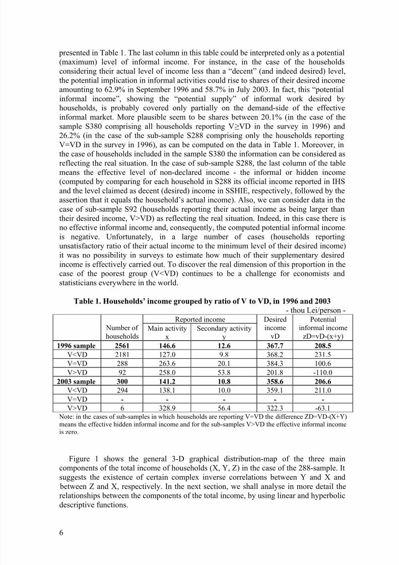
presented in Table 1. The last column in this table could be interpreted only as a potential

(maximum) level of informal income. For instance, in the case of the households

considering their actual level of income less than a “decent” (and indeed desired) level,

the potential implication in informal activities could rise to shares of their desired income

amounting to 62.9% in September 1996 and 58.7% in July 2003. In fact, this “potential

informal income”, showing the “potential supply” of informal work desired byhouseholds, is probably covered only partially on the demand-side of the effective

informal market. More plausible seem to be shares between 20.1% (in the case of the

sample S380 comprising all households reporting V≥VD in the survey in 1996) and

26.2% (in the case of the sub-sample S288 comprising only the households reporting

V=VD in the survey in 1996), as can be computed on the data in Table 1. Moreover, in

the case of households included in the sample S380 the information can be considered as

reflecting the real situation. In the case of sub-sample S288, the last column of the table

means the effective level of non-declared income - the informal or hidden income

(computed by comparing for each household in S288 its official income reported in IHS

and the level claimed as decent (desired) income in SSHIE, respectively, followed by the

assertion that it equals the household’s actual income). Also, we can consider data in thecase of sub-sample S92 (households reporting their actual income as being larger than

their desired income, V>VD) as reflecting the real situation. Indeed, in this case there is

no effective informal income and, consequently, the computed potential informal income

is negative. Unfortunately, in a large number of cases (households reporting

unsatisfactory ratio of their actual income to the minimum level of their desired income)

it was no possibility in surveys to estimate how much of their supplementary desired

income is effectively carried out. To discover the real dimension of this proportion in the

case of the poorest group (V<VD) continues to be a challenge for economists and

statisticians everywhere in the world.

Table 1. Households’ income grouped by ratio of V to VD, in 1996 and 2003

- thou Lei/person -Reported income

Number of

householdsMain activity

x

Secondary activity

y

Desired

income

vD

Potential

informal income

zD=vD-(x+y)

1996 sample 2561 146.6 12.6 367.7 208.5

V<VD 2181 127.0 9.8 368.2 231.5

V=VD 288 263.6 20.1 384.3 100.6

V>VD 92 258.0 53.8 201.8 -110.0

2003 sample 300 141.2 10.8 358.6 206.6

V<VD 294 138.1 10.0 359.1 211.0

V=VD - - - - -

V>VD 6 328.9 56.4 322.3 -63.1 Note: in the cases of sub-samples in which households are reporting V=VD the difference ZD=VD-(X+Y)means the effective hidden informal income and for the sub-samples V>VD the effective informal incomeis zero.

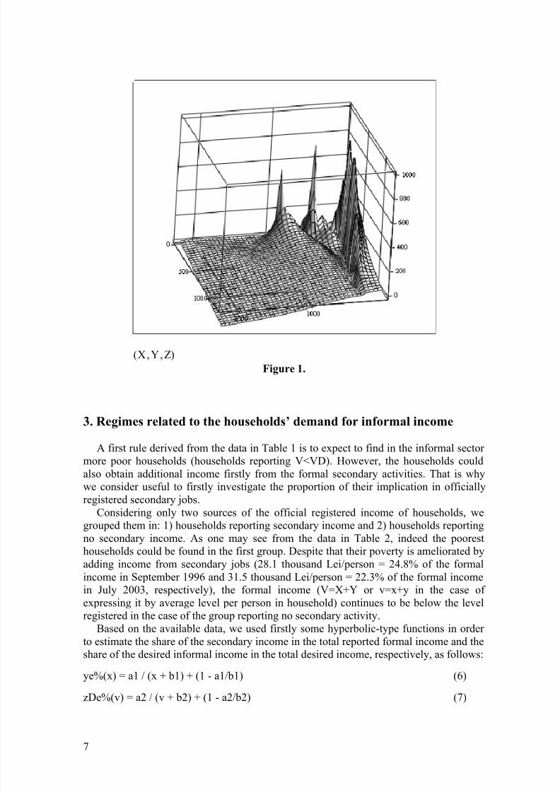
Figure 1 shows the general 3-D graphical distribution-map of the three main

components of the total income of households (X, Y, Z) in the case of the 288-sample. It

suggests the existence of certain complex inverse correlations between Y and X and

between Z and X, respectively. In the next section, we shall analyse in more detail the

relationships between the components of the total income, by using linear and hyperbolicdescriptive functions.



7

X Y, Z,( ) Figure 1.

3. Regimes related to the households’ demand for informal income

A first rule derived from the data in Table 1 is to expect to find in the informal sector

more poor households (households reporting V<VD). However, the households could

also obtain additional income firstly from the formal secondary activities. That is why

we consider useful to firstly investigate the proportion of their implication in officially

registered secondary jobs.

Considering only two sources of the official registered income of households, we

grouped them in: 1) households reporting secondary income and 2) households reporting

no secondary income. As one may see from the data in Table 2, indeed the poorest

households could be found in the first group. Despite that their poverty is ameliorated byadding income from secondary jobs (28.1 thousand Lei/person = 24.8% of the formal

income in September 1996 and 31.5 thousand Lei/person = 22.3% of the formal income

in July 2003, respectively), the formal income (V=X+Y or v=x+y in the case of

expressing it by average level per person in household) continues to be below the level

registered in the case of the group reporting no secondary activity.

Based on the available data, we used firstly some hyperbolic-type functions in order

to estimate the share of the secondary income in the total reported formal income and the

share of the desired informal income in the total desired income, respectively, as follows:

ye%(x) = a1 / (x + b1) + (1 - a1/b1) (6)

zDe%(v) = a2 / (v + b2) + (1 - a2/b2) (7)



8

where x is the average basic income (officially registered) per person in household; y -

the average secondary income (also reported) per person in household; v - the average

formal income (v=x+y) per person in household; ye%(x) - the theoretic share of

secondary income in v; zDe%(v) - the theoretic share of potential (or desired) informal

income in vD (vD=VD/number of persons in household); a1, b1, a2, b2 are coefficients

to be estimated by the regression process. In order to build the two theoretical estimationfunctions, we used as basic hypotheses: ye%(0)=1 and ye%(+∞)=c1=(1-a1/b1);

zDe%(0)=1 and zDe%(+∞)=c2=(1-a2/b2). Then, using some elementary algebraic

operations implicitly resulted the following indirect four estimation equations for the

variables y, zD, v, and vD:

ye(x) = [(b1 - a1) / a1].x + (b1

2/ a1), with ye(0) = (b1

2/a1) (8)

zDe(v) = [(b2 – a2) / a2].v + (b2

2/ a2), with zDe(0) = (b2

2/a2) (9)

and, respectively

ve(x) = (b1 . x / a1) + (b12 / a1), with ve(0) = (b12/a1) (10)

vDe(v) = (b2.v / a2) + (b2

2/ a2), with zDe(0) = (b2

2/a2) (11)

Table 2. Average income in the case of households reporting V<VD, in 1996 and

2003

- thou Lei/person -

Reported income

Number of

householdsMain activity

X

Secondary activity

Y

Desired

income

VD

Potential

informal income

ZD=VD-(X+Y)

1996 sample 2181 127.0 9.8 368.2 231.5

SI (Y=0) 1406 149.2 0.0 388.5 239.2

SII (Y>0) 775 85.4 28.1 330.5 217.0

2003 sample 294 138.1 10.0 359.1 211.0

SI (Y=0) 209 151.4 0.0 359.1 213.8

SII (Y>0) 85 109.8 31.5 346.3 205.0SI – households operating only in one activity (main or basic activity, according to the definitions included

in the SSHIE questionnaire in September 1996 and in the survey in July 2003).SII - households operating in more than one activity (main activity and secondary activities, according tothe same definitions).

Taking into account the economic significance of the data in surveys and trying to

obtain robust estimators, we selected two different ways of estimating the coefficients

(for all the regressions we used the Ordinary Least Squares standard method). Thus, to

estimate the coefficients a1 and b1 we selected as initial regression the equation:

v = (b1.x / a1) + (b1

2/ a1) + u1 (10’)

but to estimate a2 and b2 coefficients we used

zD% = a2 / (v + b2) + (1 - a2/b2) + u2 (7’)

where u1, u2 are residual variances.



9

The samples in the 1996 and 2003 surveys on which we applied the first regression

procedure (estimating a1 and b1 in the relation (10’) to introduce them in the relations

(6) and (8)) included all the households in the surveys reporting secondary income

(Y>0): S931-96 for September 1996 (there were 931 households in this sample: 775 in

the sub-group of households reporting VD>V; 88 in the sub-group reporting VD=V in

the 1996 survey; and 68 in that reporting VD<V) and S88-03 for July 2003 (there were88 households in this sample: 85 in the sub-group of households reporting VD>V and

only 3 households in the sub-group reporting secondary income in July 2003). In Table 3

are synthetically presented the basic data characterising the households’ behaviour

related to their implication in secondary activities.

The second regression procedure (estimation of a2 and b2 in the relation (7’) to

introduce them in the relations (9) and (11)) included all households reporting a level of

desired income higher than their actual income (or, equivalently, ZD>0): S2181-96 for

September 1996 (there were 2181 households in this sample) and S294-03 for July 2203

(there were 294 households in this sample). In Table 4 are synthetically presented the

basic data characterising the households’ behaviour related to their potential (expected)

implication in informal activities.

Table 3. Summary of regression equation output in the case of secondary income

Households reporting Y>0

Regression equation and

estimated coefficientsSep. 1996

(S931-96)

July 2003

(S88-03)

v=(b1/a1)x+(b12/a1)+u1

a1

(t-ratio)

(Prob(t))

11.51066025

(4.870047095)

(0.0)

2.798577816

(1.107868752)

(0.27101)

b1

(t-ratio)

(Prob(t))

14.73138239

(5.232932182)

(0.0)

3.519355431

(1.130105429)

(0.26157)

c1=(1-a1/b1) 0.21863000 0.20480387

ye(0)=ve(0)=b12/a1 18.85327361 4.42577032

Slope of ye(x)=(b1/a1)-1 0.27980342 0.25755139

Slope of ve(x)=b1/a1 1.27980342 1.25755139

R^2 (Coefficient of Det.) 0.7575092047 0.9642662622

Durbin-Watson Ratio 1.91203038621 2.29281329546

As one may see from the data reported in Tables 3 and 4 there are certain theoretical

limits in extending both secondary income and even the desired informal income. Thus,

according to the data supplied by the two surveys the minimum share of secondary

income in the total actual income (noted as c1 in Table 3, to which y% would

asymptotically tend when the main formal income per person, x, would continue to grow

very much, x → +∞) was around 21.9% of the total formal income (v=x+y or V=X+Y)

in September 1996 (in the S931-96 case) and 20.5% in July 2003 (the case of S88-03).

Also, even in the case of the desired or expected income there is a minimum share of the

informal income in the total expected income (noted as c2 in Table 4, to which zD%

would asymptotically tend when the formal registered income per person, v, would



10

continue to increase very much, x → +∞), namely around 16.4% in September 1996 and

24.7% in July 2003.

Table 4. Summary of regression equation output in the case of desired informal

income

Households reporting V<VD

Regression equation and estimated

coefficientsSep. 1996

(S2181-96)

July 2003

(S294-03)

zD%=a2/(v+b2)+(1-a2/b2) + u2

a2

(t-ratio)

(Prob(t))

96.32183317

(11.32606896)

(0.0)

73.6960427

(5.200303398)

(0.0) b2

(t-ratio)

(Prob(t))

115.2542196

(16.01823627)

(0.0)

97.88875792

(7.119246168)

(0.0)

c2=(1-a2/b2) 0.16426632 0.24714498

zDe(0)=vDe(0)=b22/a2 137.90783147 130.02338492

Slope of zDe(v)=(b2/a2)-1 0.19655343 0.32827699

Slope of vDe(v)=b2/a2 1.19655343 1.32827699

R^2 (Coefficient of Det.) 0.3994546661 0.4289735371


The estimation procedure permits (by replacing the argument v in zDe(v) function

with the sum x+ye(x)) to outline structural prototypes in the case of the two surveys. A

general representation is shown in Figure 2 (where the estimated lines for the July 2003

survey are thicker than those for the September 1996 survey). The secondary income

share in the total desired income of household is different from its share in the formal

actual income. Thus, it is asymptotically increasing as the income provided by the work

in the main activity of household increases, tending at limit to constant values: 18.3% in

September 1996 and 15.4% in July 2003, respectively. Certain behavioural regimes can

be outlined: in the case of households having low incomes from their main activity there

is a huge availability of the people to work in the informal sector; for the rich people,having considerable incomes from their work in the formal sector, their availability for

informal jobs becomes smaller; however still remain certain temptations for the richest

people to accept informal jobs in order to supplement their incomes and, perhaps, to

avoid taxation. Despite a general decreasing trend of the desired informal income share

along with the growth of the basic formal income of household, in absolute terms the

desired informal income has an ascending trend, as shown in Figure 3.



11

0 1000 20000

0.2

0.4

0.6

0.8

1

yDe%_96( )x

yDe%_03( )x

zDe%_96( )x

zDe%_03( )x

xDe%_96( )x

xDe%_03( )x

x

0 1000 20000

200

400

600

800

1000

ye_96( )x

ye_03( )x

zDe_96( )x

zDe_03( )x

x

Figure 2. Figure 3.

4. Regimes related to the households’ effective informal income

As it was already mentioned, we issued to compute indirectly the true level of

effective informal income only in the case of the September 1996 survey for the sample

S380 (comprising 288 households reporting V=VD, and 92 households reporting V>VD,

respectively). Remember that on the basis of a deeper analysis of the data in surveys we

identified three categories of total income to which the answers in households were

referring: 1) total official reported income of a household, noted as V, as it appeared inIHS, in September 1996, and in the survey of July 2003, respectively, as an aggregate

estimate noted by the data collectors on the household’s survey document (in fact this

category of total income comprised income obtained in the formal sector only, as main or

basic registered income, X, and as income from secondary but formally registered

activities, Y); 2) total desired income, noted VD, as it was reported (declared) in SSHIE

of September 1996 and in the survey of July 2003, respectively; and 3) total effective

income, noted as VR, which we computed indirectly in the case of households reporting

V≥VD (380 households in the survey of September 1996 and only 6 cases in the survey

of July 2003).

In fact, in the case of the 1996 survey, within the group of 288 households claiming

that their actual income equals their desired income, the assertion is true only for 60

cases (thus, only in the case of 60 households V=VD=VR and, consequently, they do not

effectively obtain informal income, Z=0). For the remaining 228 households within the

group S288, the assertion is a false one, when the formal reported income, V, is

compared with the level claimed as desired income, VD, but it becomes true in the case

of considering the effective (but not reported) income, VR (thus, in this case the total

effective income of household is higher than its total formal reported income,

V<VR=VD and, consequently, the household effectively obtains informal income, Z>0).

Thus, grouping now the households in the sample S380 by the criterion of effective

participation in informal sector, we obtained a new structure: a number of 228

households effectively obtaining informal income (Z>0) and 152 households noteffectively obtaining informal income (Z=0), respectively. The latter was formed by



12

adding to the group of 92 households reporting V>VD (consequently, they had no

effective informal income, Z=0) the group of 60 households coming from the former

group of 288 households initially claiming V=VD and in fact having V=VD=VR.

Table 5 presents the structure by sources of the total income within the sample S380,

this time divided in two groups according to the criterion of effective participation of

household in the informal sector. Also, based on the S380 data we computed theregression equations related to the household’s effective participation in the informal

sector. Then, in last part of the paper, the regression output will be used to obtain an

estimate for the size of informal economy in Romania, taking into account the entire

population of households and its structure by deciles according to the NIS published data

for the 1995-2002 period.

Table 5. Structure of total income in the case of the 380-sample (V≥VD)

- thou Lei/person -

Reported Income

Main

activity

x

Secondary

activities

y

Total

ReportedIncome

v=x+y

Hidden

Income

z

Total Effective

Income

vR

225.9 17.1 243.0 133.6 376.6S228 Average

% of vR 60.0% 4.5% 64.5% 35.5% 100.0%

132.7 44.6 177.3 116.6 293.9- S88 Average

% of vR 45.1% 15.2% 60.3% 39.7% 100%

283.8 - 283.8 144.1 427.9- S140 Average

% of vR 66.3% - 66.3% 33.7% 100.0%

306.1 44.0 350.1 - 350.1S152 Average

% of vR 87.4% 12.6% 100.0% - 100.0%262.1 29.2 291.3 73.3 364.6S380 Average

% of vR 71.9% 8.0% 79.9% 20.1% 100.0%

Corresponding to the data in Table 5, for the entire 380-sample the share of the

informal (hidden) income, z/vT, was around 20.1% on average and around 35.5% in the

case of the households being involved in informal activities, respectively. In other words,

the composition of a household total income in the sample S380, VT, was provided in

September 1996 by the following sources: 71.9% main activity, 8.0% secondary activity,

and 20.1% informal activity.

Thus, the last estimated share of informal income, 20.1% of total income, may be

used as a first estimation in order to obtain parameters in a general regression equation

and to characterise, for the entire population of households, the behaviour of households

related to their effective participation in the informal area. The other alternative is to

estimate the regression equation only in the case of households implied in informal

activities. Then, in order to obtain an estimate of the share of informal income at the

national level we must penalise the regression equation by the proportion of households

operating in informal sector in the total population. Thus, we must make hypothesis on

the probability that a household finds within the set of the households operating in the

informal sector. The simplest solution is to consider as a first raw estimator of this

probability the same proportion of people operating in informal sector as it is computedin the case of the sample S380. Indeed, introducing this hypothesis will additionally



13

imply to consider a similar distribution of the whole population as in the case of the

sample S380. However, taking into account that other accurate sources of more

analytical information related to the proportion of households involved in informal

activities are not available at this moment, it remains to expand the regression output

from the sample S380 to the national level by using only the available distribution of

households’ population by deciles as it is yearly published by NIS. As the empiricalavailable data in the case of the two surveys suggest, the best general fitting function to

estimate the household’s behaviour seems to be one expressing a complex inverse

relation between the average level of income provided by the work in the formal sector

(main activity and secondary activities) and the participation rate in the informal sector

(computed as the share of informal income in the total effective income in the case of the

sample S380).

Also, in the case of samples S380, as in that of S2181 already analysed in the last

section, we can affirm that households tend to involve more and more (as proportion) in

informal sector as their formal income is lower. The difference is that now, in the case of

S380, the informal income is effectively obtained as against the potential informal

income reported in the case of the 2181 sample. As one may see, the mentioned tendencyis only in relative terms, because in absolute terms the level of informal income generally

is also increasingly higher when the level of income from the formal sector grows.

Indeed, together with the level per person of formal income in absolute terms we

should consider many other factors as stimulating households to involve in the informal

sector, such as occupation, region, age, education, etc., as we proceeded in a former

special study. However, in the context of this paper certain useful conclusions could be

outlined:

People in households perceive the high rate of taxation as the main cause of the

underground activity (more than 80% of the answers in surveys demonstrate this idea).

Separating the main motivations of operating in informal sector in two groups –

“subsistence” and “enterprise”, respectively, the data in surveys suggest that the

subsistence represented a relevant reason for the households’ decision to operate in the

informal sector.

Informal activities supply a “safety valve” within the surviving strategies adopted

by the poorest households.

Participation in the informal sector seems to be not simply correlated with poverty:

in the informal activities are involved poor people (having probably a low educational

level), as well as relatively rich persons. However, their motivations are quite different.

The former are practically “forced” to operate in the informal sector (the “subsistence”

criterion), but the latter are “invited” to participate in it (the “enterprise” criterion). In

both cases, at least during the last stages of transition to a free market system inRomania, the environment was propitious due to legislative incoherence, feeble penalty

system in the cases of fraudulent activities, and existence of some accompanying

elements of proper informal activity, such as corruption, bureaucracy, etc. However, the

behaviour related to the informal economy is sometimes fundamentally different

between the two groups of population. The most synthetic expression of this idea could

be as follows: along with the growth of their formal income households tend to desire

to obtain more and more informal income in absolute terms, but at the same time its

share in the total income tends to decrease (sharply down until a reasonable average

level of formal income is obtained and slowly down in the case of the richest

households). Probably, the main reason for which the rich people could be involved in

the informal sector is provided by the attempt to avoid taxes and to follow anoptimising strategy in this matter.



14

Regarding the regimes in the case of households’ effective informal income, as a

general overview they are similar to those in the case of desired informal income, but

they are very different as regards the concrete values of the parameters and levels.

Relatively similar to the case of desired informal income in the previous section of

this paper, we used again the hypothesis of a hyperbolic-type function for z%(v). This

time z means the effective informal income, in order to make difference from the desiredinformal income, zD. Also, in order to estimate the coefficients we selected as basic

regression equation that expressing the share of informal income in the total household’s

income, z%, as being correlated with the level of the formal income in household, as

follows:

z% = a / (v + b) + (1 - a/b) + u (12)

where a, b are coefficients to be estimated and u is residual variance.

Now, using the estimated values of coefficients we can write, along with changes in

the level of formal income, the expected trajectories, as follows:

ze% = a / (v + b) + (1 - a/b) (12’)

ze(v) = [(b – a) / a].v + (b

2/ a), with ze(0) = (b

2/a) (13)

and, respectively

vRe(v) = (b / a).v + (b

2/ a), with vRe(0) = ze(0) = (b

2/a) (14)

The samples of the September 1996 survey on which we applied the regression

procedure were S380 and the sub-sample S228, respectively (in the case of the 2003

survey there is no possibility to evaluate the effective informal income). Table 6

synthetically presents the basic data characterising the households’ behaviour related to

their effective informal income. From the data in this table resulted a limit-value for the

share z%(+∞) of around 2.1% in the case of the 380-sample (representing an estimator

of the average value in the case of the entire population of households) and 9.4% in the

case of considering only the households involved in the informal sector.

Table 6. Summary of regression equation output in the case of real informal

income

Households reporting V≥VDRegression equation and estimated

coefficients S380-96 S228-96

z%=a/(v+b)+(1-a/b) + ua

(t-ratio)

(Prob(t))

40.20288127

(5.78891877)

(0.0)

52.28482256

(4.515511099)

(0.00001)

b

(t-ratio)

(Prob(t))

41.08227834

(6.649225468)

(0.0)

57.730209

(5.463029131)

(0.0)

c=(1-a/b) 0.02140575 0.0943247311

vCr= b2/(2a-b) 42.91973684 71.15322701

ze(0)=ve(0)=b2/a 41.98091132 63.74272433

Slope of ze(v)=(b/a)-1 0.02187398 0.10414851

Slope of vRe(v)=b/a 1.021873981 1.1041485114R^2 (Coefficient of Det.) 0.256104055 0.3420802227



15


A general representation of the estimation function for S380 and S228 is shown in

Figure 4 (where the estimated lines for the sub-sample S228, solid line and dashed line,

are thicker than those for the sample S380). Also, on graphs are marked the critical

values of v, vCr380 and vCr228, respectively, for which the informal income shareequals the share of formal income in the total real income of household. One may see an

important positive shift of the function z%(v) to the upper side of graph in the case of

translation from S380 to S228.

0 50 100 150 2000

0.2

0.4

0.6

0.8

1

c380c228

z380e% v( )

z228e% v( )

v380e% v( )

v228e% v( )

vCr380 vCr228

v

Figure 4.

Remember that in the case of the sample S380 the function of informal income share

reflects indirectly also the impact of changing the proportion of households operating in

the informal sector (or, equivalently: the impact of changing the probability that ahousehold is involved in the informal sector) along with the growth of the formal income

per person in household. Consequently, it could be used directly to expand the estimation

procedure to the national level. An impediment remains: it is implicitly supposed the

same distribution of the entire population by formal income as in the case of the S380

sample. On the other hand, the sample S228 comprises only the households that obtain

informal income. In this case, to simply extrapolate the z%(v) function to the entire set of

households’ population is not a good solution. Thus, firstly we have to amend the z%(v)

function by multiplying it with the probability function computed, for instance, by

deciles, as we shall proceed in the next section of the paper.

It is also interesting to compare the estimated function for informal income in the case

of the sample S2181, comprising only “pure” potential (desired) informal incomereported by households, and that in the case of the S228 sample, including only “pure”



16

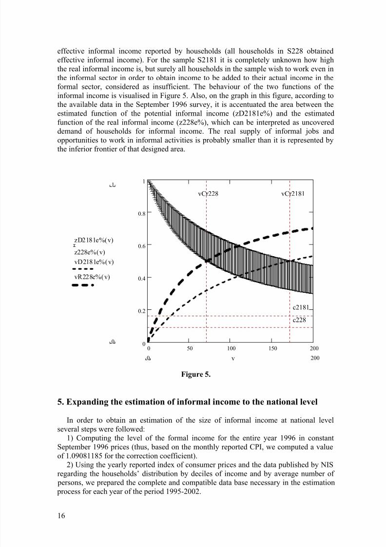
effective informal income reported by households (all households in S228 obtained

effective informal income). For the sample S2181 it is completely unknown how high

the real informal income is, but surely all households in the sample wish to work even in

the informal sector in order to obtain income to be added to their actual income in the

formal sector, considered as insufficient. The behaviour of the two functions of the

informal income is visualised in Figure 5. Also, on the graph in this figure, according tothe available data in the September 1996 survey, it is accentuated the area between the

estimated function of the potential informal income (zD2181e%) and the estimated

function of the real informal income (z228e%), which can be interpreted as uncovered

demand of households for informal income. The real supply of informal jobs and

opportunities to work in informal activities is probably smaller than it is represented by

the inferior frontier of that designed area.

0 50 100 150 2000

0.2

0.4

0.6

0.8

11

0

c2181

c228

zD2181e% v( )

z228e% v( )

vD2181e% v( )

vR228e% v( )

2000

vCr228 vCr2181

v

Figure 5.

5. Expanding the estimation of informal income to the national level

In order to obtain an estimation of the size of informal income at national level

several steps were followed:

1) Computing the level of the formal income for the entire year 1996 in constant

September 1996 prices (thus, based on the monthly reported CPI, we computed a value

of 1.09081185 for the correction coefficient).

2) Using the yearly reported index of consumer prices and the data published by NIS

regarding the households’ distribution by deciles of income and by average number of

persons, we prepared the complete and compatible data base necessary in the estimation

process for each year of the period 1995-2002.



17

3) Extrapolating the output of the regression equation selected in the case of the

sample S380 (supposed to reflect correctly the entire population of households regarding

their behaviour related to the participation in the informal sector) to estimate the level of

real income and, consequently, that of the real informal income at the level of the entire

population of households structured by deciles of formal income per person in Romania

for each year of the analysed period.4) Extrapolating the output of the regression equation used already in the case of the

sample S228 to the entire population in the analysed period in order to obtain an estimate

for the superior value of informal income share (it is plausible only in the case when all

households are involved in informal activities, as it is the case of the sample S228).

5) Amending the last estimating equation by adding a supplementary equation

concerning the probability that a person in a household is involved in the informal

economy. This was estimated by regressing within the sample S380 the proportion of

persons in households obtaining effectively informal income in the total number of the

deciles in which they are located (the total number of this special category of household

is just the sample S228):

p = a.d + b + u (15)

and from which the equation (13) is rewritten as

zpe(v) = ze(v).pe(d) (13’)

where d are deciles (d=1…10); pe(d)=ad+b is the estimation equation of the probability

that a person in a household is involved in the informal economy, p; a and b are the

estimated coefficients, and u is residual variance in the equation (15). Table 7

synthetically presents the basic data characterising the regression equation (15).

6) Comparing the three estimating procedures and their outputs.

Table 7. Summary of the regression equation (15)

Regression equation and estimated

coefficients

Households with Z>0 (S228-96)

within sample S380-96

p = a.d + b + u

a

(t-ratio)

(Prob(t))

-0.02987557576

(-2.037636312)

(0.07595)

b

(t-ratio)(Prob(t))

0.7067002667

(7.768108416)(0.00005)

R^2 (Coefficient of Det.) 0.34167008

Durbin-Watson Ratio 1.23928982856

Very synthetically, the conclusion is that over the period 1995-2002 the informal

income increased in Romania from around 18% in the total real income of households in

1995 to near 21% in 2002, with a maximum level of around 22% in 1999 and 2000.

Under the very improbable hypothesis of a generalised participation in informal

activities, the computed share value grew from 29% in 1995 to near 32% in 2002 (with a

minimum value of 28% in 1996 and a maximum value of 33.7% in 2000).

Deeper interesting conclusions could be extracted in the case of analysing by decilesthe dynamic process of involvement in the informal sector. Appendix 2 presents the three



18

matrices comprising the shares of informal income within the total income in the case of

all deciles for each year of the period 1995-2002, corresponding to the three estimating

methods. In Appendix 3 is presented the contribution of deciles to the total informal

income at national level, also corresponding to the three methods.

Figures 6 and 7 show the estimated dynamics of the informal income share based on

the two estimation functions over the period 1995-2002 (the year 1995 is denoted as 1and 2002 as 8), and their relatively strong direct correlation with the distribution of

population number by deciles, respectively. z%M, represents the yearly average of the

informal income share in the total income at national level, resulted from the regression

equation based on the S380 sample and zp%M from that computed on the S228 sample

amended by the probability function, respectively. The detailed data for the years of the

analysed period are presented in Table 8.

1 2 3 4 5 6 7 80.16

0.18

0.2

0.22

0.24

z%M j

zp%M j

j

0.06 0.074 0.089 0.1 0.12 0.13 0.15 0.160

0.1

0.2

0.3

0.4

0.5

z%D i j,

zp%D i j,

n%i j,

Figure 6. Figure 7.

Table 8 Average shares of informal income in the total income of households

over the period 1995-2002

Years z%M zp%M

1995 18.2 18.31996 17.3 17.5

1997 20.2 20.0

1998 20.8 20.5

1999 22.1 21.6

2000 22.3 21.7

2001 21.2 20.6

2002 20.7 20.2

Finally, Figures 8 and 9 show as graphical representations the strong inversecorrelations emerging in the case of grouping the households’ population by deciles,



20

Albu, L.-L., Kim, B.-Y., and Duchene, G. (2002):”Households’ Activities in Informal

Economy: Size and Behavioural Aspects”, in: Romanian Journal of Economic

Forecasting, Vol. 3-4 (11-12), Bucharest.

Albu, L.-L. and Nicolae, M. (2002): “Use of Households Survey Data to Estimate the

Size of the Informal Economy in Romania”, in: The Informal Economy in the EU

Accession Countries: Size, Scope, Trends and Challenges to the Process of EU Enlargement , Network for Integration of Central and Eastern-European Countries into

the European Union, March, Sofia.

Albu, L.-L., Tarhoaca, C., and Ivan-Ungureanu, C. (2001): Study of informal economy

in Romania, CRPE, IRIS, Bucharest.

Allingham, M.G. and Sandmo, A. (1972): “Income Tax Evasion: A Theoretical

Analysis”, Journal of Public Economics, November, 1(3-4).

Archambault, E. and Greffe, X. (1984): Les économies non officielles, La Decouverte.

Bhattacharyya, D.K. (1999): On the Economic Rationale of Estimating the Hidden

Economy, The Economic Journal 109/456, pp. 348-359.

Blades, Derek (1982): “The Hidden Economy and the National Accounts”, OECD

(Occasional Studies), Paris, pp. 28-44.Cagan, Phillip (1958): “The Demand for Currency Relative to the Total Money

Supply,” Journal of Political Economy, 66:3, pp. 302-328.

Clotfelter, C.T. (1983): ”Tax Evasion and Tax Rates: An Analysis of Individual

Returns”, Review of Economics and Statistics, Vol. 65.

Cowell, F. (1985):”Tax Evasion with Labour Income”, Journal of Public Economics,

February, 26(1).

Cowell, F. (1990): Cheating the government , Cambridge MA: MIT Press.

Daianu, D. and Albu, L.-L. (1997):”Institutions, Strain and the Underground

Economy”. International Conference on the Importance of the Underground Economy in

Economic Transition, University of Zagreb. The Davidson Institute Working Paper

Series, 98.

Dobrescu, E. (1996): Macromodels of the Romanian Transition, EXPERT Publishing

House, Bucharest.

Duchene, G., (1999): “Les revenues informels en Roumanie. Estimation par enquete”,

in: Revue d’etudes comparatives Est-Ouest, vol. 30, no. 4, Paris.

Duchene, G. (coordinator), Adair, P., Albu, L.-L., Ivan-Ungureanu, C., Neff, R., and

Tanase, F. (1998): Informal economy in Romania, ACE-Phare Project, ROSES, Paris,

September.

Feige, Edgar L. (1989) (ed.): The underground economies. Tax evasion and

information distortion. Cambridge, New York, Melbourne, Cambridge University Press.

Feldstein, M. (ed.) (1983): Behavioural Simulation Methods in Tax Policy Analysis,The University of Chicago Press.

Fortin, B. and Hung, N.M. (1987): “Poverty trap and the hidden labour market”,

Economics Letters, No. 25.

Fortin, B. and Lacroix, G. (1994): “Labour supply, tax evasion and the marginal cost

of public funds. An empirical investigation”, Journal of Public Economics, 55(3),

November.

French, R., Balaita, M. and Ticsa M. (1999): “Estimating The Size And Policy

Implications Of The Underground Economy In Romania”, US Department of the

Treasury, Office of Technical Assistance, Bucharest, August.

Frey, Bruno S. and Hannelore Weck-Hannemann (1984): The hidden economy as an

“unobserved” variable, European Economic Review, 26/1, pp. 33-53.



21

Frey, Bruno S. and Werner Pommerehne (1984): The hidden economy: State and

prospect for measurement, Review of Income and Wealth, 30/1, pp. 1-23.

Gibson, B. and Kelley, B. (1994):”A Classical Theory of the Informal Sector”, The

Manchester School, Vol. LXII, 1.

Gutmann, Pierre M. (1977): “The Subterranean Economy ,” Financial Analysts

Journal, 34:1, pp. 24-27.Hénin, P.-Y. (1986): Equilibres avec rationnement d'une économie a planification

centralisée et secteur paralléle: une analyse macroéconomique, Revue d'économie

politique, No. 3.

Isachsen, A.J., and Strom, S. (1980): The hidden economy: The labour market and tax

evasion, Scandinavian Journal of Economics, 82.

Jung, Y.H., Snow, A., and Trandel, G.A. (1994):”The evasion and the size of the

underground economy”, Journal of Public Economics, Vol. 54.

Kesselman, J.R., (1989): Income tax evasion: An intersectoral analysis, Journal of

Public Economics, Vol. 38.

Lackó Mária (1997): Do power consumption data tell the story? (Electricity Intensity

and the hidden economy in Post-Socialist countries), Laxenburg: International Institutefor Applied Systems Analysis (IIASA), working paper.

Lemieux, T., Fortin, B., and Fréchette, P. (1994):”The Effect of Taxes on Labour

Supply in the Underground Economy”, The American Economic Review, March, 84(1).

Pencavel, J.H. (1979), A Note on Income Tax Evasion, Labour Supply, and Non-

linear Tax Schedules, Journal of Public Economics, Vol. 12.

Pestieau, P. (1989): L' Economie souterraine, Hachette, Pluriel.

Pestieau, P. and Possen, U. M. (1991): "Tax evasion and occupational choice",

Journal of Public Economics, Vol. 45.

Portes, A., Castells, M. and Benton, L.A. (1989): The informal economy: Studies in

advanced and less developed countries, Baltimore, MD: John Hopkins University Press.

Sandmo, A. (1981): Income Tax Evasion, Labour Supply, and the Equity-Efficiency

Tradeoff, Journal of Public Economics, 16(3), December.

Smith, S. (1986): Britain's Shadow Economy, Clarendon Press, Oxford.

Schneider, Friedrich (1994): Can the shadow economy be reduced through major tax

reforms? An empirical investigation for Austria, Supplement to Public Finance/

Finances Publiques, 49, pp. 137-152.

Schneider, Friedrich (2002): “The Size and Development of the Shadow Economies

and Shadow Economy Labour Force of 22 Transition and 21 OECD Countries: What Do

We Really Know?”, in: The Informal Economy in the EU Accession Countries: Size,

Scope, Trends and Challenges to the Process of EU Enlargement , Network for

Integration of Central and Eastern-European Countries into the European Union, March,Sofia.

Schneider, Friedrich and Dominik Enste (2000): Shadow Economies: Size, Causes,

and Consequences, The Journal of Economic Literature, 38/1, pp. 77-114.

Schneider, F. and Neck, R. (1992): “The development of the shadow economy under

changing tax systems and structures: some (tentative) empirical results for Austria”,

International Seminar in Public Economics, Escorial (Madrid), June 11-12.

Smith, S. (1986): Britain's Shadow Economy, Clarendon Press.

Tanzi, Vito (1982) (ed.): The underground economy in the United States and abroad ,

Lexington (Mass.), Lexington.

Thomas, J., (1992): Informal Economic Activity, Harvester Wheatsheaf, London.

Tobin, J. (1969): Comment on Borch and Feldstein, Review of Economic Studies, Vol.36.



22

Watson, H. (1985): Tax evasion and labour markets, Journal of Public Economics,

Vol. 27.

Yaniv, G. (1994): Tax Evasion and the Income Tax Rate: a Theoretical Re-

examination, Public Finance, Vol. 49.

Yitzhaki, S. (1974): A Note on Income Tax Evasion: A Theoretical Analysis, Journal

of Public Economics, 3(2), May.*** National Institute of Statistics (1996-2003): Population income, expenditure and

consumption, Romanian Statistical Yearbook 1996-2003, Bucharest.



23

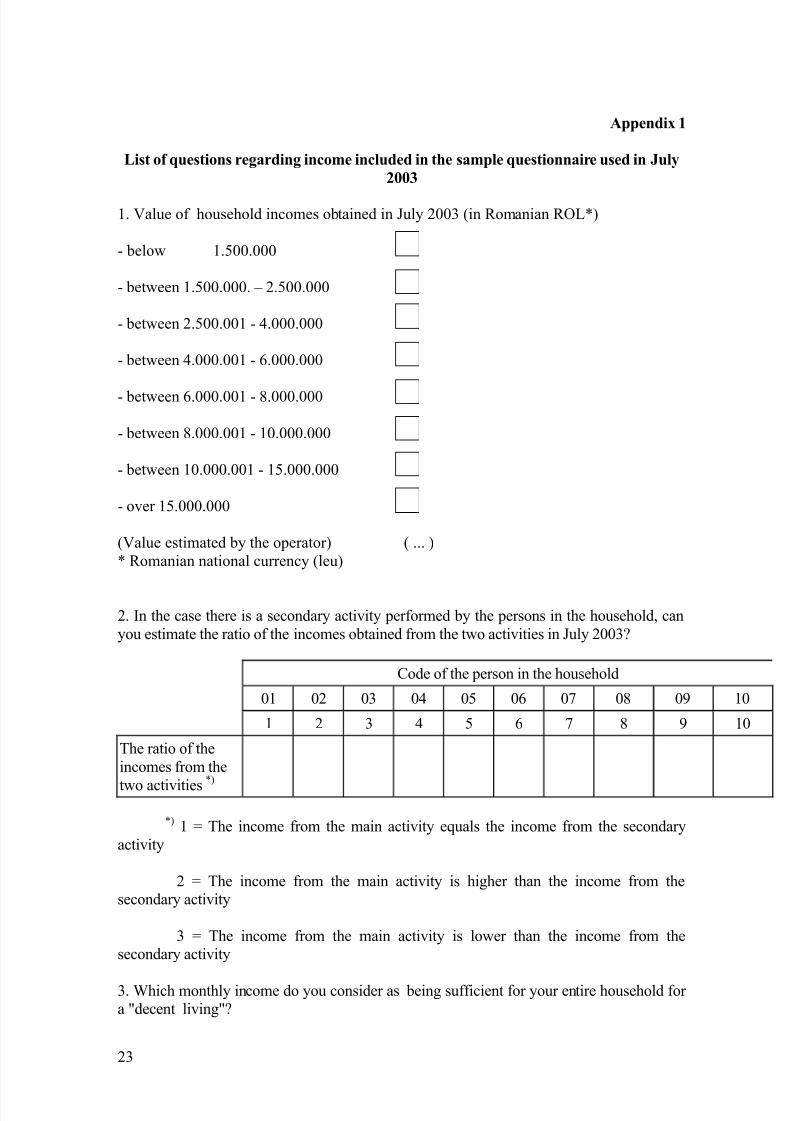
Appendix 1

List of questions regarding income included in the sample questionnaire used in July

2003

1. Value of household incomes obtained in July 2003 (in Romanian ROL*)

- below 1.500.000

- between 1.500.000. – 2.500.000

- between 2.500.001 - 4.000.000

- between 4.000.001 - 6.000.000

- between 6.000.001 - 8.000.000

- between 8.000.001 - 10.000.000

- between 10.000.001 - 15.000.000

- over 15.000.000

(Value estimated by the operator) ( ... )

* Romanian national currency (leu)

2. In the case there is a secondary activity performed by the persons in the household, can

you estimate the ratio of the incomes obtained from the two activities in July 2003?

Code of the person in the household

01 02 03 04 05 06 07 08 09 10

1 2 3 4 5 6 7 8 9 10

The ratio of the

incomes from the

two activities*)

*) 1 = The income from the main activity equals the income from the secondary

activity

2 = The income from the main activity is higher than the income from the

secondary activity

3 = The income from the main activity is lower than the income from the

secondary activity

3. Which monthly income do you consider as being sufficient for your entire household for

a "decent living"?



24

Amount └┴┴┴┴┴┴┴┴┘ lei

List of questions regarding income included in the sample questionnaire used in

September 1996 (SSHIE Survey)

1. In the case where exists a second activity that is carried out by the persons from the

household, could you estimated the ratio of the obtained incomes from these two

activities?

Code of person within the household

01 02 03 04 05 06 07 08 09 10

1 2 3 4 5 6 7 8 9 10

The ratio of the incomes from

these two activities*) *) 1= the income from the first activity is equal to the income from the second activity

2 = the income from the first activity is higher than the income from the second

activity

3 = the income from the first activity is lower than the income from the second activity

2. Which is the monthly income that will be sufficient to the whole household for a

“decent living”?

The amount …………… lei

3. How do you consider that is your existing total income in ratio to the one that would

be sufficient for a “decent” living? You should encircle the right answer.

Low Almost equal Higher

1 2 3



25

Appendix 2

Shares of informal income in total income by deciles

H1 Estimations under the hypothesis of S380 regression equation

Years 1995 1996 1997 1998 1999 2000 2001 2002

Deciles D1 0.383 0.360 0.406 0.415 0.438 0.454 0.380 0.393

D2 0.283 0.266 0.303 0.313 0.330 0.342 0.314 0.310

D3 0.244 0.229 0.263 0.273 0.286 0.299 0.279 0.271

D4 0.217 0.206 0.236 0.246 0.257 0.269 0.256 0.251

D5 0.196 0.186 0.216 0.224 0.234 0.246 0.238 0.234

D6 0.179 0.171 0.198 0.206 0.214 0.225 0.222 0.217

D7 0.163 0.156 0.182 0.188 0.196 0.203 0.204 0.199

D8 0.147 0.140 0.163 0.170 0.177 0.182 0.182 0.177

D9 0.127 0.121 0.142 0.146 0.154 0.156 0.158 0.150

D10 0.086 0.083 0.097 0.100 0.110 0.109 0.105 0.100Average 0.182 0.173 0.202 0.208 0.221 0.223 0.212 0.207

H2 Estimations under the hypothesis of S288 regression equation amended

by adding the regression equation of probability (S228 in S380)

Years 1995 1996 1997 1998 1999 2000 2001 2002

Deciles D1 0.407 0.385 0.429 0.438 0.459 0.474 0.404 0.416

D2 0.303 0.287 0.321 0.331 0.346 0.358 0.331 0.328

D3 0.257 0.244 0.274 0.283 0.295 0.308 0.289 0.282

D4 0.224 0.214 0.241 0.250 0.259 0.270 0.259 0.254

D5 0.198 0.189 0.215 0.221 0.230 0.240 0.233 0.230D6 0.175 0.168 0.190 0.197 0.204 0.213 0.210 0.206

D7 0.154 0.149 0.169 0.174 0.180 0.186 0.186 0.182

D8 0.134 0.129 0.146 0.151 0.157 0.161 0.161 0.157

D9 0.113 0.109 0.124 0.127 0.132 0.133 0.134 0.129

D10 0.080 0.078 0.087 0.089 0.095 0.095 0.092 0.089

Average 0.183 0.175 0.200 0.205 0.216 0.217 0.206 0.202

H3 Estimations under the hypothesis of a generalized informal economy

(based on the equation of regression used in the case of sample S228)

Years 1995 1996 1997 1998 1999 2000 2001 2002

Deciles D1 0.503 0.480 0.526 0.535 0.556 0.571 0.501 0.513

D2 0.401 0.383 0.422 0.433 0.450 0.463 0.434 0.430

D3 0.359 0.343 0.380 0.390 0.404 0.418 0.397 0.389

D4 0.330 0.317 0.350 0.362 0.373 0.387 0.373 0.367

D5 0.306 0.295 0.329 0.338 0.348 0.362 0.353 0.349

D6 0.286 0.277 0.308 0.317 0.327 0.339 0.335 0.330

D7 0.268 0.260 0.290 0.297 0.306 0.314 0.315 0.309

D8 0.249 0.241 0.268 0.276 0.284 0.290 0.290 0.285

D9 0.226 0.218 0.244 0.249 0.258 0.260 0.262 0.254

D10 0.176 0.173 0.190 0.193 0.205 0.204 0.199 0.194

Average 0.290 0.280 0.312 0.319 0.334 0.337 0.324 0.318



Appendix 3

Shares of informal income in total income by years

H1 Estimations under the hypothesis of S380 regression equation

Years 1995 1996 1997 1998 1999 2000 2001 2002

Deciles D1 0.137 0.134 0.137 0.137 0.139 0.137 0.128 0.126

D2 0.117 0.117 0.117 0.115 0.117 0.112 0.110 0.109

D3 0.106 0.109 0.110 0.108 0.110 0.105 0.100 0.100

D4 0.103 0.103 0.104 0.103 0.103 0.098 0.096 0.097

D5 0.097 0.096 0.098 0.096 0.097 0.096 0.096 0.100

D6 0.094 0.093 0.092 0.094 0.094 0.091 0.092 0.092

D7 0.089 0.090 0.089 0.090 0.089 0.093 0.092 0.094

D8 0.087 0.087 0.087 0.089 0.087 0.091 0.096 0.095

D9 0.085 0.086 0.083 0.086 0.085 0.089 0.095 0.094

D10 0.085 0.084 0.082 0.084 0.080 0.088 0.095 0.093Total 1.000 1.000 1.000 1.000 1.000 1.000 1.000 1.000

H2 Estimations under the hypothesis of S288 regression equation amended

by adding the regression equation of probability (S228 in S380)

Years 1995 1996 1997 1998 1999 2000 2001 2002

Deciles D1 0.150 0.147 0.152 0.153 0.156 0.154 0.146 0.143

D2 0.128 0.128 0.129 0.127 0.129 0.124 0.123 0.122

D3 0.113 0.116 0.118 0.116 0.118 0.113 0.109 0.109

D4 0.107 0.107 0.108 0.107 0.107 0.102 0.101 0.101

D5 0.097 0.096 0.098 0.097 0.097 0.096 0.096 0.100D6 0.091 0.090 0.089 0.090 0.091 0.088 0.089 0.089

D7 0.083 0.084 0.083 0.083 0.083 0.086 0.085 0.087

D8 0.078 0.078 0.077 0.079 0.077 0.081 0.085 0.084

D9 0.074 0.076 0.072 0.074 0.073 0.077 0.081 0.081

D10 0.079 0.078 0.074 0.075 0.070 0.078 0.085 0.084

Total 1.000 1.000 1.000 1.000 1.000 1.000 1.000 1.000

H3 Estimations under the hypothesis of a generalized informal economy

(based on the equation of regression used in the case of sample S228)

Years 1995 1996 1997 1998 1999 2000 2001 2002

Deciles D1 0.122 0.119 0.124 0.124 0.127 0.124 0.117 0.114

D2 0.108 0.108 0.110 0.107 0.110 0.105 0.103 0.102

D3 0.101 0.103 0.105 0.103 0.105 0.100 0.096 0.096

D4 0.099 0.100 0.101 0.099 0.100 0.095 0.093 0.094

D5 0.095 0.094 0.097 0.095 0.096 0.094 0.094 0.098

D6 0.094 0.094 0.093 0.094 0.095 0.091 0.092 0.091

D7 0.091 0.092 0.091 0.092 0.092 0.095 0.093 0.095

D8 0.091 0.092 0.091 0.093 0.091 0.095 0.099 0.098

D9 0.092 0.095 0.090 0.092 0.092 0.096 0.101 0.101

D10 0.106 0.104 0.100 0.101 0.094 0.105 0.113 0.112

Total 1.000 1.000 1.000 1.000 1.000 1.000 1.000 1.000

Romania's Economy

Documents

Transcript of Romania's Economy