Role of Turbulent Prandtl Number on Heat Flux at ... · American Institute of Aeronautics and...

American Institute of Aeronautics and Astronautics

1

Role of Turbulent Prandtl Number on Heat Flux at Hypersonic Mach Numbers

X. Xiao*, J. R. Edwards†, and H. A. Hassan‡ North Carolina State University, Raleigh, NC 27695-7910

and

R. L. Gaffney, Jr.§ NASA Langley Research Center, Hampton, VA 23681-2199

A new turbulence model suited for calculating the turbulent Prandtl number as part of

the solution is presented. The model is based on a set of two equations: one governing the

variance of the enthalpy and the other governing its dissipation rate. These equations were

derived from the exact energy equation and thus take into consideration compressibility and

dissipation terms. The model is used to study two cases involving shock wave/boundary

layer interaction at Mach 9.22 and Mach 5.0. In general, heat transfer prediction showed

great improvement over traditional turbulence models where the turbulent Prandtl number

is assumed constant. It is concluded that using a model that calculates the turbulent Prandtl

number as part of the solution is the key to bridging the gap between theory and experiment

for flows dominated by shock wave/boundary layer interactions.

Nomenclature

Ch, Ch,1-Ch,11 = model constants

h = enthalpy

2"~h = enthalpy variance

M = Mach number

k = turbulence kinetic energy

* Research Assistant Professor, Dept. of Mechanical and Aerospace Engineering, Member AIAA † Associate Professor, Dept. of Mechanical and Aerospace Engineering, Associate Fellow AIAA ‡ Professor, Dept. of Mechanical and Aerospace Engineering, Associate Fellow AIAA. § Aerospace Engineer, Hypersonic Air Breathing Propulsion Branch, Senior Member AIAA. Copyright©2005 By the American Aeronautics and Astronautics, Inc. All rights reserved.

https://ntrs.nasa.gov/search.jsp?R=20080006846 2018-09-05T22:39:32+00:00Z


2

P = pressure

Pr = Prandtl number

qi = turbulent heat flux

Sij = strain tensor

T = temperature

ui = velocity

α = heat diffusivity

β = deflection angle of shock generator

ν = kinematic viscosity

ρ = density

ζ = enstrophy

h∈ = dissipation rate of enthalpy variance

Subscript

0 = stagnation conditions

t = turbulent

w = wall

� = free stream

I. Introduction

Present simulation of turbulent flows involving shock wave/boundary layer interaction invariably over-estimate

heat flux by almost a factor of two.1 One possible reason for such performance is a result of the fact that the

turbulence models employed make use of Morkovin’s hypothesis.2 This hypothesis is valid for non-hypersonic

Mach numbers and moderate rates of heat transfer. At hypersonic Mach numbers, high rates of heat transfer exist in

regions where shock wave/boundary layer interactions are important. For such flows, temperature fluctuations,

which are as important as velocity fluctuations at the higher Mach numbers, play a major role in determining the


3

wall heat flux and their effects must explicitly be taken into consideration. As a result, one should not expect

traditional turbulence models to yield accurate results.

The goal of this investigation is to explore the role of a variable Prandtl number formulation in predicting the

heat flux in flows dominated by strong shock wave/boundary layer interactions. The intended applications involve

flows in the absence of combustion such as those encountered in supersonic inlets. This can be achieved by adding

equations for the temperature (enthalpy) variance and its dissipation rate. Such equations can be derived from the

exact Navier-Stokes equations. Traditionally, modeled equations (see, for example, Ref. 3,4) are based on the low

speed energy equation where the pressure gradient term and the term responsible for energy dissipation are ignored.

It is clear that such assumptions are not valid for hypersonic flows.

The approach used here is based on the procedure used in deriving the k-ζ model,5 in which the exact equations

that governed k, the variance of velocity, and ζ, the variance of vorticity, were derived and modeled. For the

variable turbulent Prandtl number, the exact equations that govern the temperature (enthalpy) variance and its

dissipation rate are derived and modeled term by term. The resulting set of equations are free of damping and wall

functions and are coordinate-system independent. Moreover, modeled correlations are tensorially consistent and

invariant under Galilean transformation.

Two flat plate experiments were used to determine model constants. The first is the Mach (M) 9.2 experiments

of Coleman and Stollery6, which was conducted in a hypersonic gun tunnel at Imperial College. The second is the

M=8.3 experiments of Kussoy et al.7 which were conducted in the Ames 3.5 Foot Hypersonic Wind Tunnel Facility.

This turned out to be a major undertaking because of the different instrumentations and because no accuracy

estimates of heat transfer measurement were provided. In order to put things in proper perspective, it is noted that

recent heat transfer measurements8 on an elliptic cone in the Arnold Engineering Development Center (AEDC)

Tunnel B estimated uncertainties in excess of ±10%. The model was validated by recent non-intrusive

measurements by Schülein9 of flows involving shock wave/boundary layer interactions at M = 5. The measurements

were carried out at the Ludwig Tube Facility at DLR. Oil-film interferometry techniques were used to measure skin

friction while an infrared camera system was used for heat transfer measurements.

The recent measurements of Schülein were a repeat of an earlier experiment10 which did not include heat transfer

measurements or skin friction measurements in the separated flow region. Calculations of the earlier experiments

were carried out by Nance and Hassan11 using a k-ζ two-equation and an abbreviated stress model. It was concluded


4

in Ref. 10 that there was a need to develop turbulence models capable of predicting the turbulent Prandtl number as

part of the solution.

It is shown in this study that a variable Prandtl number formulation results in significant improvement of heat

transfer predictions in the presence of shock wave/boundary layer interactions. However, the new model has

insignificant influence on wall pressure and skin friction distributions.

II. Formulation of the Problem

1. Governing equations

The energy equation can be written as

hi

ii

i

Sx

q

Dt

DPhu

xh

tDt

Dh ≡+∂∂−=

∂∂+

∂∂= φρρρ )()( (1)

where i

i x

Tq

∂∂−= λ

j

iij x

ut

∂∂=φ

m

mijijij x

uSt

∂∂−= µδµ

3

22

∂∂

+∂∂=

i

j

j

iij x

u

x

uS

21

(2)

and ρ is the density, h is the enthalpy, P is the pressure, iu is the velocity and λ and µ are the coefficients of thermal

conductivity and molecular viscosity. Noting that


5

Dt

DRT

Dt

DTR

Dt

DP ρρ += (3)

and using the relation TCh P= and the conservation of mass equation, Eq. (1) can be re-written as

+

∂∂−+

∂∂−−= φγργρ

i

i

i

i

x

q

x

uh

Dt

Dh)1( , vP CC /=γ (4)

where PC and vC are the specific heats at constant pressure and constant volume.

The mean energy equation follows from Eq. (1) as

( ) ( ) ( )jji

ii

i

uhxx

q

Dt

PDuh

xh

t′′′′

∂∂−+

∂∂−=

∂∂+

∂∂ ρφρρ ~~~

(5)

where

∈+∂∂= ρφ

j

iij x

ut

~; νζ=∈ (6)

where ν is the kinematic viscosity and ζ is the enstrophy.

Equation (4) was the starting point for deriving an equation for the enthalpy variance and its dissipation

rate. The exact equations are given in the Appendix, while the modeled equations are:

( )

∂′′∂+

∂∂=′′

∂∂+′′

∂∂

jht

jj

j x

hC

xhu

xh

t

)2/~

()(2/

~~)2/~

(2

2,22 αγαρρρ

( ) ( ) )/(~

34

//2 ,,, ρµγρρµγ jtj

kkjti

itj

ij qx

Sqx

qx

S∂∂−

∂∂+

∂∂+

i

i

x

uh

∂∂′′−−

~~)1( 2ργ hh

iit hC

x

hq ∈−′′+

∂∂− ργζγµ 2

4,,

~2

~ (7)

where

j

tjt x

hq

∂∂−=

~

, αρ


6

[ ]89.0/5.0 thht kC ντα +=

hh h ∈′′= /~ 2τ

2

∂

′′∂=∈i

h x

hα (8)

and where h∈ is the rate of dissipation of the enthalpy variance, α is the diffusivity, and

kt kCkC τνζν µµ ≡= /2

is the turbulent kinematic viscosity.

The modeled equation for the dissipation of enthalpy variance is

=∈∂∂+∈

∂∂

)~()( hjj

h uxt

ρρk

jjkjkhh x

ubC

∂∂

−∈−

~

35,

δρ

jj

h x

h

x

hkC

∂∂

∂′′∂+

~~ 2

6, ρ

∂∈∂+

∂∂+

j

hth

j xC

x)( 7, αγα

jh

jth x

hqC

∂∂+

τ,

8,

+∈−

k

h

h

hh

CC

ττγρ 10,9,

+∈+ 0.0,max11, Dt

DP

PDt

DC hh

ρρ ( 9 )

with

ijij

ij kb δ

ρτ

32+= , jiij uu ′′′′−= ρτ (10)

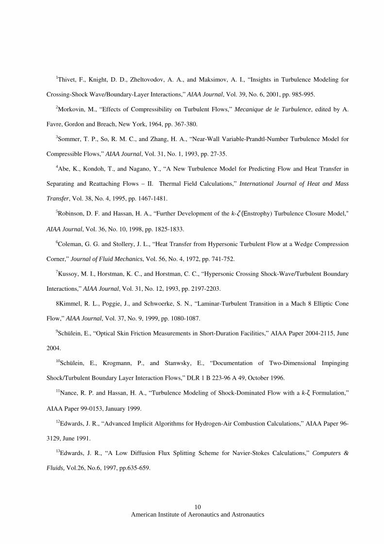
The constants, Ch, …, Ch,11 are model constants and are given in Table 1. The turbulent Prandtl number is

defined as

ttt /Pr = (11)

The choice of tα merits further elaboration. It was indicated in Ref. 4 that experiments in simple shear flows

showed that the appropriate time scale for temperature fluctuations is proportional to the arithmetic average of hτ


7

and kτ . This is the basis for the modeling indicated in Eq. 8. It should be noted that, traditionally3,4, the time scale

of temperature fluctuations is taken as the geometric average of hτ and kτ .

2. Numerical Procedure

A modification of REACTMB12, a code that has been developed at North Carolina State University over the last

several years, is used to set constants and validate the model. It employs a second order ENO upwind method based

on the Low-diffusion Flux-Splitting of Edwards13 to discretize the inviscid fluxes while central differences are

employed for the viscous and diffusion terms. Planar relaxation is used to advance the solution in time.

III. Results and Discussion

The solutions computed using the model are shown first with the data from the 15 deg ramp experiment of

Coleman and Strollery. In this experiment no flow separation was indicated. The remaining comparisons will be

made with Schülein two-dimensional flow measurements for deflection angles β of 10 and 14 degrees. Flow

separation was observed for both of these angles.

The free stream conditions for the experiments of Coleman and Strollery are: M=9.2, Re=47×106/m, T0= 1070K,

T� = 64.5K and Tw = 295K. It has been shown in Ref. 11 that use of 241 × 141 Cartesian grid with constant spacing

in the x (flow) direction and geometric spacing in the y (normal) direction resulted in a grid resolved solution and

this grid is employee in the present calculations. Values of y+ are less than 0.2. Figures 1 and 2 compare the pressure

distribution and wall heat flux for constant and variable Prandtl number calculations. As is seen from Fig. 1 the

pressure distribution is essentially independent of the turbulent Prandtl number. The variable Prandtl number

calculations are in good agreement with experiment in the pressure rise region and both calculations underpredict

the heat flux in the recovery region. The recovery region has always been difficult to predict using Reynolds

Averaged Navier-Stokes (RANS) equations. Better results are obtained when a hybrid Large Eddy

Simulation/Reynolds Averaged Navier-Stokes (LES/RANS) formulation is employed14.

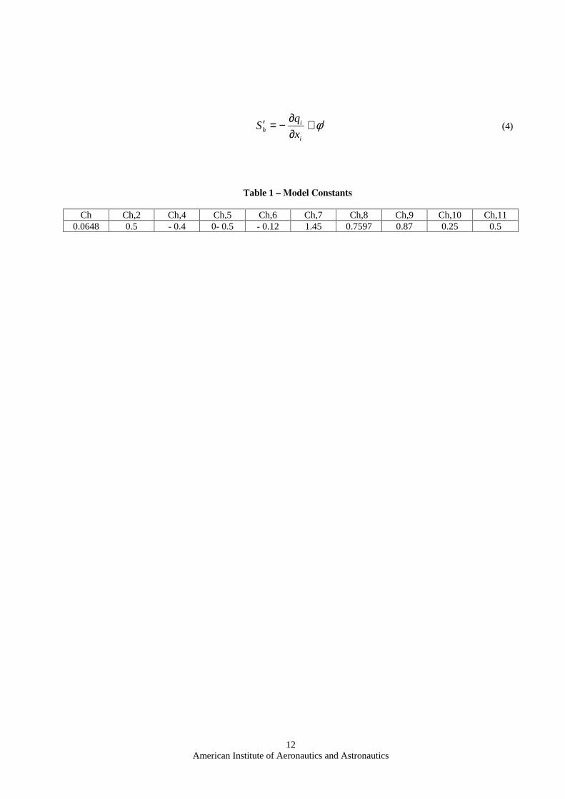
The experimental setup of the Schülein experiment is shown in Fig. 3. A shock generator is mounted on the

upper wall and the resultant oblique shock wave interacts with the turbulent boundary layer growing on the flat plate

along the lower wall. The free-stream conditions in the test section were: M=5, unit Reynolds number = 37×106/m,

T0 = 410K, P0=2.12 MPa and a wall temperature of 300±5 K. Three grids are used in this investigation: a coarse


8

151×141, medium 243×141, and fine 301×141. Results employing the medium and fine gave grid independent

solutions. All results presented below employ the fine grid.

The calculations were limited to a region ahead of the point where the reflected shock impinges on the upper

surface. This assumption makes it possible to use an extrapolation boundary condition at the outflow. Without this

assumption, one would be forced to consider the upper wall in the calculations.

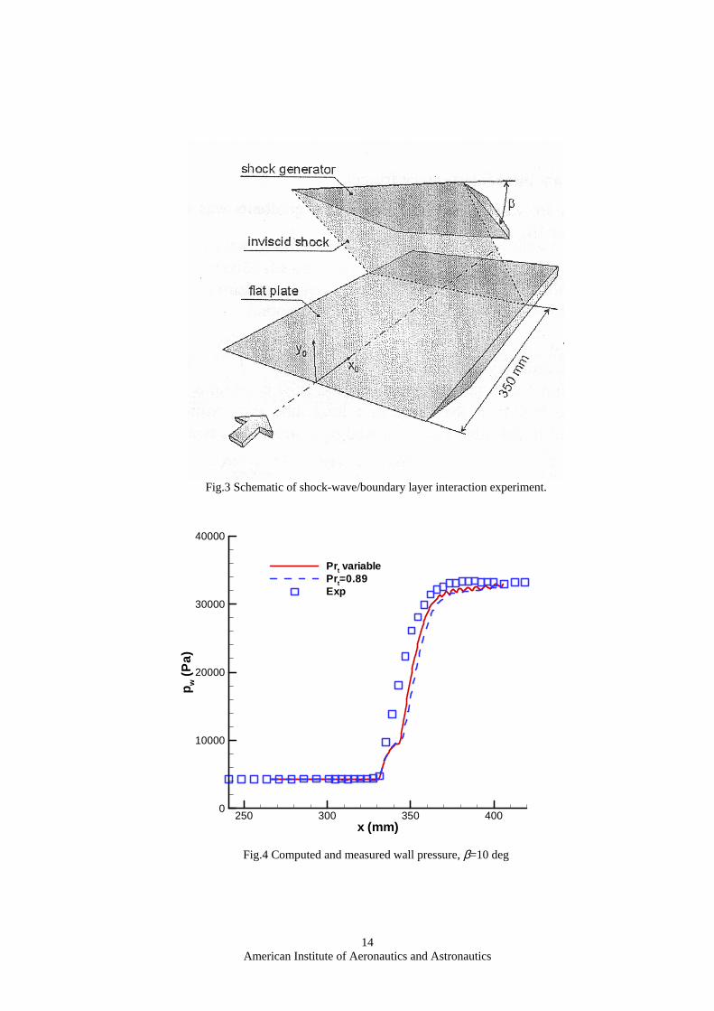
Figures 4-6 compare predictions of surface pressure, wall shear stress and wall heat flux while Figs. 7 and 8

compare temperature and velocity at x = 376 mm for β =10 deg. It is seen from Figs. 4 and 5 that the results are

almost identical for both constant and variable turbulent Prandtl numbers. Both calculations underpredict the

pressure in the separated region.

The oil-film interferometry technique cannot be used to determine the extent of the separated region. Instead,

conventional oil-film visualization was used to deduce the start and end of the separated region. It is seen from Fig.

5 that the extent of separation is well predicted. However, some discrepancies are noted in predicting the wall shear

stress in the recovery region. The calculations are consistent with the fact that the τw should decrease in the constant

pressure region. As is seen from Fig. 4, measurements suggest that the pressure is approximately constant after

x=370mm station. It is not clear why the experiment indicates in the wall shear stress downstream of this location.

Figure 6 shows that constant Prandtl number calculations overpredict peak heating by a factor of 2. As is seen

from the figure, the variable Prt results represent a definite improvement over constant Prt results. The slight

oscillation in the calculated results are attributed to the fact that the shock does not lie along a grid line. The

oscillations can be reduced or eliminated by increasing the numerical damping of the numerical scheme. As is seen

from Fig. 9, the convergence history indicates that the small oscillations are not an indication of lack of iterative

convergence.

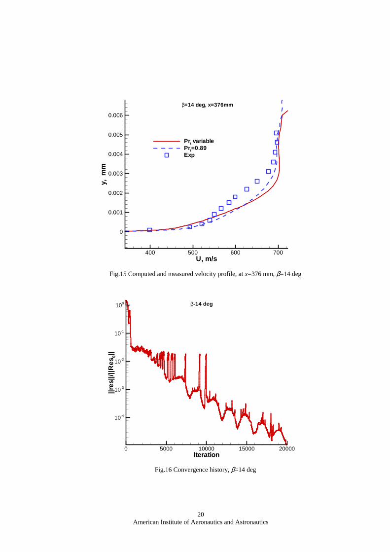
Figures 7 and 8 show that both temperature and velocity profile are in fair good agreement with experiment. The

fact that the variable Prandtl number formulation results in more realistic heat flux estimates is a direct result of the

fact that temperature distribution for the variable Prandtl number is in better agreement with experiment near the

wall.

Figure 10 shows a contour plot of Prt in the neighborhood of the separated region. In the separated region, Prt is

about 1.0. As a result, both constant and variable Prt solutions yield similar results as indicated in Fig. 6.

Downstream of that region, Prt is greater than 1,which is responsible for the reduction in the heat flux compared


9

with the constant Prt results. Outside the boundary layer, the first term in the expression for αt is much less than

89.0/tν and thus Prt asymptotes to 1.78. This has no real physical significance because the temperature is

essentially constant outside the boundary layer.

Figures 11-17 compare similar predictions for the β = 14 degree case. Similar remarks can be made regarding

this case. Experimental measurements show more oscillations in the data.

IV. Concluding Remarks

A new approach has been developed for calculating the turbulent Prandtl number as part of the solution. The

approach is based on a two-equation model for the enthalpy variance and its dissipation rate. All of the correlations

that appear in the exact equations that govern the enthalpy variance and its dissipation rate are modeled in order to

ensure the incorporation of relevant physics into the model equations.

The new formulation is used to study flows characterized by shock wave/boundary layer interactions. In general

heat flux calculations showed dramatic improvements while surface pressures and wall shear stress were unaffected

by the variable Prandtl number formulation.

When comparing pressure, skin friction and heat flux measurements, the highest errors are associated with heat

flux measurements. Despite the discrepancy between computed and measured heat flux, the key to bridging the gap

between theory and experiment in flows dominated by shock wave/boundary layer interactions is to employ better

measurement techniques and use variable turbulent Prandtl number formulations. It has always been difficult for

RANS solutions to reproduce the correct flow behavior in the recovery regions. Hybrid LES/RANS approaches have

better prediction capabilities and should be used in future investigations.

V. Acknowledgment

The authors would like to acknowledge partial support under NASA Grant NAG1-03030 and Air Force Contract

FA9101-04-C-0015.

VI. References


10

1Thivet, F., Knight, D. D., Zheltovodov, A. A., and Maksimov, A. I., “Insights in Turbulence Modeling for

Crossing-Shock Wave/Boundary-Layer Interactions,” AIAA Journal, Vol. 39, No. 6, 2001, pp. 985-995.

2Morkovin, M., “Effects of Compressibility on Turbulent Flows,” Mecanique de le Turbulence, edited by A.

Favre, Gordon and Breach, New York, 1964, pp. 367-380.

3Sommer, T. P., So, R. M. C., and Zhang, H. A., “Near-Wall Variable-Prandtl-Number Turbulence Model for

Compressible Flows,” AIAA Journal, Vol. 31, No. 1, 1993, pp. 27-35.

4Abe, K., Kondoh, T., and Nagano, Y., “A New Turbulence Model for Predicting Flow and Heat Transfer in

Separating and Reattaching Flows – II. Thermal Field Calculations,” International Journal of Heat and Mass

Transfer, Vol. 38, No. 4, 1995, pp. 1467-1481.

5Robinson, D. F. and Hassan, H. A., “Further Development of the k-ζ (Εnstrophy) Turbulence Closure Model,"

AIAA Journal, Vol. 36, No. 10, 1998, pp. 1825-1833.

6Coleman, G. G. and Stollery, J. L., “Heat Transfer from Hypersonic Turbulent Flow at a Wedge Compression

Corner,” Journal of Fluid Mechanics, Vol. 56, No. 4, 1972, pp. 741-752.

7Kussoy, M. I., Horstman, K. C., and Horstman, C. C., “Hypersonic Crossing Shock-Wave/Turbulent Boundary

Interactions,” AIAA Journal, Vol. 31, No. 12, 1993, pp. 2197-2203.

8Kimmel, R. L., Poggie, J., and Schwoerke, S. N., “Laminar-Turbulent Transition in a Mach 8 Elliptic Cone

Flow,” AIAA Journal, Vol. 37, No. 9, 1999, pp. 1080-1087.

9Schülein, E., “Optical Skin Friction Measurements in Short-Duration Facilities,” AIAA Paper 2004-2115, June

2004.

10Schülein, E., Krogmann, P., and Stanwsky, E., “Documentation of Two-Dimensional Impinging

Shock/Turbulent Boundary Layer Interaction Flows,” DLR 1 B 223-96 A 49, October 1996.

11Nance, R. P. and Hassan, H. A., “Turbulence Modeling of Shock-Dominated Flow with a k-ζ Formulation,”

AIAA Paper 99-0153, January 1999.

12Edwards, J. R., “Advanced Implicit Algorithms for Hydrogen-Air Combustion Calculations,” AIAA Paper 96-

3129, June 1991.

13Edwards, J. R., “A Low Diffusion Flux Splitting Scheme for Navier-Stokes Calculations,” Computers &

Fluids, Vol.26, No.6, 1997, pp.635-659.


11

14Xiao, X., Edwards, J. R., and Hassan, H. A., “Blending Functions in Hybrid Large Eddy/Reynolds Averaged

Navier-Stokes Simulations,” AIAA Journal, Vol.42, No. 12, 2004, pp.2508-2515.

VII. Appendix

1. Exact Equation for Enthalpy Variance:

( ) [ ] [ ] hjjj

jjj

Shhuxx

huhhu

xh

t′′+′′′′

∂∂−

∂∂′′′′−=′′

∂∂+′′

∂∂

2/~

2/~~2/

~ 2ρρρρ (1)

where

φξh

xh

Dt

DphSh

i

ih ′′+

∂∂′′−′′=′′ (2)

2. Exact Equation for the Dissipation Rate of Enthalpy Variance:

kjk

jjkk

j

k

j

kjh

t xx

h

x

hu

x

h

x

h

x

u

x

u

x

h

x

h

D

D

∂∂∂

∂′′∂′′+

∂∂

∂′′∂

∂′′∂

+∂∂

∂∂

∂′′∂+∈

~2

~2

~2

2

ραραραρ

jkk

j

kjj x

h

x

h

x

u

x

h

xu

∂′′∂

∂′′∂

∂′′∂

+

∂

′′∂∂∂′′+ ραρα 2

2

( )

′′′′

∂∂−

′∂∂

∂′′∂= hu

x

S

xx

hj

j

h

kk

ρρρ

ρα 12 (3)

where


12

φ′+∂∂−=′

i

ih x

qS (4)

Table 1 – Model Constants

Ch Ch,2 Ch,4 Ch,5 Ch,6 Ch,7 Ch,8 Ch,9 Ch,10 Ch,11

0.0648 0.5 - 0.4 0- 0.5 - 0.12 1.45 0.7597 0.87 0.25 0.5


13

x(m)

p w/p

∞

-0.02 0 0.02 0.04 0.060

1

2

3

4

5

6

7

8

9

10

11

12

13

14

Prt variablePrt=0.89Exp

M∞=9.2

Fig.1 Computed and measured pressure distribution, 15 deg ramp

x(m)

q w/q

∞

-0.05 0 0.050

1

2

3

4

5

6

7

8

9

10

11


M∞=9.2

Fig.2 Computed and measured heat flux, 15 deg ramp


14

Fig.3 Schematic of shock-wave/boundary layer interaction experiment.

x (mm)

p w(P

a)

250 300 350 4000

10000

20000

30000

40000


Fig.4 Computed and measured wall pressure, β=10 deg


15

x (mm)

τ w(P

a)

300 350 400

0

100

200

300

400 Prt variablePrt=0.89Exp

Fig. 5 Computed and measured wall shear stress, β=10 deg

x (mm)

q w(W

/m2)

300 350 400

20000

40000

60000

80000


Fig.6 Computed and measured wall heat flux, β=10 deg


16

T, K

y,m

m

100 150 200 250

0

0.0005

0.001

0.0015

0.002


β=10 deg, x=376mm

Fig. 7 Computed and measured temperature profile at x=376 mm, β=10 deg

U, m/s

y,m

m

450 500 550 600 650 700 750

0

0.001

0.002

0.003


β=10 deg, x=376mm

Fig. 8 Computed and measured velocity profile at x=376 mm, β=10 deg


17

Iteration

||Res

||/||R

es0||

0 5000 1000010-6

10-5

10-4

10-3

10-2

10-1

100 β=10 deg

Fig.9 Convergence history, β=10 deg

x, m

log 1

0(y

/1m

)

0.3 0.35 0.4

-6

-5

-4

-3

-2

prt

1.81.711.621.531.441.351.261.171.080.990.90.810.720.630.540.450.360.270.180.090

Fig.10 Contours of turbulent Prandtl number, β=10 deg


18

x (mm)

p w(P

a)

250 300 350 4000

10000

20000

30000

40000

50000

60000


Fig.11 Computed and measured wall pressure, β=14 deg

x (mm)

τ w(P

a)

250 300 350 400

0

200

400

600 Prt variablePrt=0.89Exp

Fig.12 Computed and measured wall shear stress, β=14 deg


19

x (mm)

q w(W

/m2)

300 350 400

20000

40000

60000

80000

100000

120000

140000

160000


Fig.13 Computed and measured wall heat flux, β=14 deg

T, K

y,m

m

150 200 250 300

0

0.001

0.002

0.003

0.004

0.005


β=14 deg, x=376mm

Fig.14 Computed and measured temperature profile, at x=376 mm, β=14 deg


20

U, m/s

y,m

m

400 500 600 700

0

0.001

0.002

0.003

0.004

0.005

0.006


β=14 deg, x=376mm

Fig.15 Computed and measured velocity profile, at x=376 mm, β=14 deg

Iteration

||res

||/||R

es0|

|

0 5000 10000 15000 20000

10-4

10-3

10-2

10-1

100 β-14 deg

Fig.16 Convergence history, β=14 deg


21

x, m

log

10(

y/1

m)

0.3 0.35 0.4

-6

-5

-4

-3

-2

prt

1.81.711.621.531.441.351.261.171.080.990.90.810.720.630.540.450.360.270.180.090

Fig.17 Contours of turbulent Prandtl number, β=14 deg

Role of Turbulent Prandtl Number on Heat Flux at ... · American Institute of Aeronautics and...

Documents

Transcript of Role of Turbulent Prandtl Number on Heat Flux at ... · American Institute of Aeronautics and...