
Role of the hydrological cycle in regulating the planetary ... · 1Colorado Research Associates,...
13
Nonlinear Processes in Geophysics, 12, 741–753, 2005 SRef-ID: 1607-7946/npg/2005-12-741 European Geosciences Union © 2005 Author(s). This work is licensed under a Creative Commons License. Nonlinear Processes in Geophysics Role of the hydrological cycle in regulating the planetary climate system of a simple nonlinear dynamical model K. M. Nordstrom 1 , V. K. Gupta 2,3 , and T. N. Chase 2,4 1 Colorado Research Associates, 3380 Mitchell Lane, Boulder, Colorado 80301, USA 2 Cooperative Institute for Research in the Environmental Sciences, University of Colorado, Boulder, Colorado 80309, USA 3 Department of Civil and Environmental Engineering, University of Colorado, Boulder, Colorado 80309, USA 4 Department of Geography, University of Colorado, Boulder, Colorado 80309, USA Received: 12 July 2004 – Revised: 15 March 2005 – Accepted: 16 March 2005 – Published: 29 July 2005 Part of Special Issue “Nonlinear deterministic dynamics in hydrologic systems: present activities and future challenges” Abstract. We present the construction of a dynamic area fraction model (DAFM), representing a new class of mod- els for an earth-like planet. The model presented here has no spatial dimensions, but contains coupled parameteriza- tions for all the major components of the hydrological cy- cle involving liquid, solid and vapor phases. We investigate the nature of feedback processes with this model in regu- lating Earth’s climate as a highly nonlinear coupled system. The model includes solar radiation, evapotranspiration from dynamically competing trees and grasses, an ocean, an ice cap, precipitation, dynamic clouds, and a static carbon green- house effect. This model therefore shares some of the charac- teristics of an Earth System Model of Intermediate complex- ity. We perform two experiments with this model to deter- mine the potential effects of positive and negative feedbacks due to a dynamic hydrological cycle, and due to the relative distribution of trees and grasses, in regulating global mean temperature. In the first experiment, we vary the intensity of insolation on the model’s surface both with and without an active (fully coupled) water cycle. In the second, we test the strength of feedbacks with biota in a fully coupled model by varying the optimal growing temperature for our two plant species (trees and grasses). We find that the negative feed- backs associated with the water cycle are far more powerful than those associated with the biota, but that the biota still play a significant role in shaping the model climate. third ex- periment, we vary the heat and moisture transport coefficient in an attempt to represent changing atmospheric circulations. 1 Introduction Earth’s climate has remained surprisingly stable since its for- mation four and a half billion years ago, a situation which has led to the hypothesis that the Earth Climate System (ECS) Correspondence to: K. M. Nordstrom ([email protected]) is a self-regulating complex system. It has been proposed (Lovelock, 1972; Lovelock and Margulis, 1974) that the bio- sphere plays a key role in this climatic self-regulation. How- ever, the presence of water on earth was a prerequisite for life to have originated, and for it to have evolved since then. Indeed, water is the fundamental substance supporting the existence of all life on earth and connecting it to the environ- ment. The global hydrological cycle involving the movement of fresh water through the complete planetary system and the coexistence of water in three phases (liquid, solid and vapor) distinguishes Earth from apparently lifeless planets such as Mars and Jupiter. These broad observations suggest that the water cycle plays a key role in climatic self-regulation on earth with or without the existence of a biosphere, and serve as a focus for this article. We will demonstrate, using a relatively simple nonlinear dynamical model, that the presence of an active water cycle on earth can play a key role in the regulation and evolution of its temperatures. Oceans act as low-albedo heat sinks and, in conjunction with the atmosphere, circulate to bring heat to the poles. Polar ice caps reflect a large percentage of in- coming radiation. Clouds block both short-wave radiation entering the atmosphere and long-wave radiation leaving it, while precipitation and evaporation processes move heat and water between the ground, oceans and the atmosphere. Evap- otranspiration processes couple all of this to biota, which in turn are an important contributor to the carbon cycle. These and other global bio-geochemical processes consist of pos- itive and negative nonlinear feedbacks, and provide a basis for understanding the role of the hydrological cycle in the self-regulation of planetary temperatures. Our simple nonlinear model, called a Dynamic Area Frac- tion Model (DAFM), has zero spatial dimensions (0-D) (Nordstrom et al., 2004; Nordstrom, 2002). It is a box model, in which the key biophysical processes involving the water cycle interact dynamically. The boxes of this model expand or contract dynamically as a result of these interactions. The 0-D structure of the model greatly simplifies specification
Transcript of Role of the hydrological cycle in regulating the planetary ... · 1Colorado Research Associates,...
Nonlinear Processes in Geophysics, 12, 741–753, 2005SRef-ID: 1607-7946/npg/2005-12-741European Geosciences Union© 2005 Author(s). This work is licensedunder a Creative Commons License.
Nonlinear Processesin Geophysics
Role of the hydrological cycle in regulating the planetary climatesystem of a simple nonlinear dynamical model
K. M. Nordstrom 1, V. K. Gupta2,3, and T. N. Chase2,4
1Colorado Research Associates, 3380 Mitchell Lane, Boulder, Colorado 80301, USA2Cooperative Institute for Research in the Environmental Sciences, University of Colorado, Boulder, Colorado 80309, USA3Department of Civil and Environmental Engineering, University of Colorado, Boulder, Colorado 80309, USA4Department of Geography, University of Colorado, Boulder, Colorado 80309, USA
Received: 12 July 2004 – Revised: 15 March 2005 – Accepted: 16 March 2005 – Published: 29 July 2005
Part of Special Issue “Nonlinear deterministic dynamics in hydrologic systems: present activities and future challenges”
Abstract. We present the construction of a dynamic areafraction model (DAFM), representing a new class of mod-els for an earth-like planet. The model presented here hasno spatial dimensions, but contains coupled parameteriza-tions for all the major components of the hydrological cy-cle involving liquid, solid and vapor phases. We investigatethe nature of feedback processes with this model in regu-lating Earth’s climate as a highly nonlinear coupled system.The model includes solar radiation, evapotranspiration fromdynamically competing trees and grasses, an ocean, an icecap, precipitation, dynamic clouds, and a static carbon green-house effect. This model therefore shares some of the charac-teristics of an Earth System Model of Intermediate complex-ity. We perform two experiments with this model to deter-mine the potential effects of positive and negative feedbacksdue to a dynamic hydrological cycle, and due to the relativedistribution of trees and grasses, in regulating global meantemperature. In the first experiment, we vary the intensity ofinsolation on the model’s surface both with and without anactive (fully coupled) water cycle. In the second, we test thestrength of feedbacks with biota in a fully coupled model byvarying the optimal growing temperature for our two plantspecies (trees and grasses). We find that the negative feed-backs associated with the water cycle are far more powerfulthan those associated with the biota, but that the biota stillplay a significant role in shaping the model climate. third ex-periment, we vary the heat and moisture transport coefficientin an attempt to represent changing atmospheric circulations.
1 Introduction
Earth’s climate has remained surprisingly stable since its for-mation four and a half billion years ago, a situation which hasled to the hypothesis that the Earth Climate System (ECS)
Correspondence to:K. M. Nordstrom([email protected])
is a self-regulating complex system. It has been proposed(Lovelock, 1972; Lovelock and Margulis, 1974) that the bio-sphere plays a key role in this climatic self-regulation. How-ever, the presence of water on earth was a prerequisite forlife to have originated, and for it to have evolved since then.Indeed, water is the fundamental substance supporting theexistence of all life on earth and connecting it to the environ-ment. The global hydrological cycle involving the movementof fresh water through the complete planetary system and thecoexistence of water in three phases (liquid, solid and vapor)distinguishes Earth from apparently lifeless planets such asMars and Jupiter. These broad observations suggest that thewater cycle plays a key role in climatic self-regulation onearth with or without the existence of a biosphere, and serveas a focus for this article.
We will demonstrate, using a relatively simple nonlineardynamical model, that the presence of an active water cycleon earth can play a key role in the regulation and evolutionof its temperatures. Oceans act as low-albedo heat sinks and,in conjunction with the atmosphere, circulate to bring heatto the poles. Polar ice caps reflect a large percentage of in-coming radiation. Clouds block both short-wave radiationentering the atmosphere and long-wave radiation leaving it,while precipitation and evaporation processes move heat andwater between the ground, oceans and the atmosphere. Evap-otranspiration processes couple all of this to biota, which inturn are an important contributor to the carbon cycle. Theseand other global bio-geochemical processes consist of pos-itive and negative nonlinear feedbacks, and provide a basisfor understanding the role of the hydrological cycle in theself-regulation of planetary temperatures.
Our simple nonlinear model, called a Dynamic Area Frac-tion Model (DAFM), has zero spatial dimensions (0-D)(Nordstrom et al., 2004; Nordstrom, 2002). It is a box model,in which the key biophysical processes involving the watercycle interact dynamically. The boxes of this model expandor contract dynamically as a result of these interactions. The0-D structure of the model greatly simplifies specification

742 K. M. Nordstrom et al.: Role of the hydrological cycle in regulating the planetary climate system
of spatial variabiltiy of biophysical processes and forcings.It allows us to test to what degree they contribute to theself-regulation of the planetary climate.
Although it is possible to generalize the DAFM frameworkto include a larger number of boxes than considered here, orto explicitly include spatial dimensions, we believe that it isnecessary to first understand the role of the key dynamicalprocesses involved in climatic self-regulation in their sim-plest form. Insights in this paper will provide a foundation onwhich to base further generalizations. Our motivation for thiswork is to understand all zero-order dynamical processes andtheir interactions through the water cycle while still main-taining maximum simplicity. The complexity of a climatemodel increases with added spatial dimensions, additionalprocesses, or boxes, all of which increase the number of in-teracting parameters. Many of these parameters are poorlyknown. A complete error analysis or even a consistent inter-pretation of cause and effect becomes more difficult as modelcomplexity increases.
On the other hand, models with low spatial dimensions anda small number of boxes have been used quite successfullyin a variety of climate applications (Budyko, 1969; Paltridge,1975; Watson and Lovelock, 1983; Ghil and Childress, 1987;Harvey and Schneider, 1987; O’Brian and Stephens, 1995;Houghton et al., 1995; Svirezhev and von Bloh, 1998). How-ever, they generally lack many of the basic interactions whichdefine our climate system. These can include an interactivehydrological cycle, cryosphere, biosphere, and biogeochem-ical cycles. We will present the construction of a DAFM rep-resenting a new class of 0-D model of an earth-like planetwith coupled parameterizations for all the major componentsof the hydrological cycle involving liquid, solid and vaporphases. This model therefore shares some of the character-istics of an Earth System Model of Intermediate complexity(EMICS) (Claussen et al., 2002). We leave the addition of adynamic carbon feedback for future work, though the carbongreenhouse effect is included in static form.
We begin by describing the construction of our model inSect.2, and discuss feedbacks and parameter estimation inSects.3 and4, respectively. In Sect.5, we present two sim-ple experiments with this model and the results for each. InSect.6, we conclude.
2 Model description
A model of even this “limited” complexity contains a rela-tively large number of variables, and for this discussion con-sistent naming conventions are important for clarity. Sec-tion 2.1 describes these conventions. Representing such acomplex system with a DAFM requires establishing dynam-ics for energy balance and for other intrinsic variables, andit requires adding area fraction dynamics for oceans and icecaps. We shall describe the representation of these compo-nents as well as other aspects of the hydrological cycle inSects.2.2–2.6.
2.1 Naming conventions
This model consists of 6 regions and subregions, and localvariables associated with each region are labelled with a sub-script i to denote regional dependence. This subscript cantake the valuet for trees,g for grasses,d for bare ground(“dirt”), o for ocean,acc for accumulation zone, orabl forablation zone. If the subscript refers to the ice sheet as awhole, it is denoted by a capital letterI . Global mean quan-tities without regional dependence are denoted by an overbar,as inT .
On each region, there are four prognostic variables to up-date. These are the region sizeai , the temperatureTi , the pre-cipitable waterwi , and the soil moisturesi . Each region alsohas several diagnostic variables associated with it, each ofwhich affects the update for the prognostic variables. Thesediagnostic variables include precipitationPi , evaporationEi ,cloud albedoAci , greenhouse greynessνi , and cloudinessaci .
Finally, each region includes a transport term for each ofthe three transverse fluxes, heat, atmospheric moisture, andsoil moisture. These are denoted byFHi , whereH is the fluxin question. The DAFM adjustment termsKHi , which willbe introduced below and are necessary to establish globalconservation of quantitiesH , follow a similar convention.
2.2 Energy balance
The DAFM framework used here was introduced inNord-strom et al.(2004) to remove the assumption of perfect localhomeostasis through the albedo-dependent local heat transferequation in the Daisyworld model ofWatson and Lovelock(1983). It was pointed out byWeber(2001) that the regu-lation of local temperatures in Daisyworld, or homeostasis,was proscribed by the biota independently of solar forcing.Additionally, the strength of the model’s homeostatic behav-ior, its main result, was forced to depend on an arbitrary pa-rameter associated with the heat transport. The DAFM for-mulation enabled us to interpret the Daisyworld heat trans-port parameter physically, thus removing the artificiality inits parameter set. This representation also resulted in globaltemperature self-regulation similar to that in Daisyworld, de-spite the removal of the assumption of perfect local home-ostasis. Under the DAFM framework used inNordstromet al. (2004), we stipulated local temperature adjustmentsdue to solar radiative forcing in each box, and constrainedthe total energy of the planet to satisfy energy conservation.We will follow the same approach here for each box of ourDAFM climate model.
We use a constant heat capacity across the system,cp inthe energy balance equation, rather than differentiating it be-tween land and ocean boxes. Estimates ofcp vary widely(Harvey and Schneider, 1987) for both ocean and land, butwe takecp=3×10¹⁰J/m2K as a representative value. Ac-counting for variations incp by region will be addressed infuture versions of the model. The results of the model inits steady state are relatively insensitive to the value ofcp,
K. M. Nordstrom et al.: Role of the hydrological cycle in regulating the planetary climate system 743
though integration paths in time vary, sincecpdt provides aneffective timescale for temperature update.
Regional temperatures in the model update through radia-tive balance
cpTi = Rin,i − Rout,i + FT i + KT i (1)
in which Rin is the net incoming shortwave radiation at thesurface,Rout is the net outgoing longwave radiation from thesurface,FT i represents the interregional heat transfer,KT i
is the DAFM term explained below in Eqs. (9) and (10). Ti
represents a total derivative of temperature in time. Thesequantities are defined to be
Rin,i = SLA′
i (1 − aciAci) (2)
Rout,i = σ [(1 − aci)(1 − νi)T4i + aciT
4c ] (3)
FT i = DT (T − Ti) (4)
with S the insolation of the present-day earth averaged over asphere,L the ratio of the model insolation toS, A′
i the localmean co-albedo for a region,aci the region mean cloudiness,Aci the region mean cloud albedo,σ the Stefan-Boltzmannfactor for blackbody radiation, 1−νi the greenhouse factorin the longwave greybody term,Tc the cloud-top tempera-ture, andcp the column-integrated heat capacity perm2 ofthe earth.DT is a coefficient of heat transfer, and the formof FT i is used for simplicity (Budyko, 1969). While it isclear that using a single coefficientDT for every region ofthe model is technically not accurate, it is also clear that wemust do so in order that theFT i terms integrate to zero overthe globe. The error thus introduced should be investigatedin a future model by using a more realistic representation ofheat transport. It is important to note that in a DAFM,Rin,i ,Rout,i , andFT i are terms with specific physical significance,whereasKT i is present for accounting purposes.
2.3 Dynamic areas
The update of local variables in a DAFM is relativelystraightforward, since it is a box model, except for the ad-dition of an extra term to account for the movement of localboundaries. This term incorporates the adjustment of locally-conserved quantities like water mass and energy, and it per-forms an instantaneous averaging over the region.
To understand the term, consider a system with two re-gions of areasa1 anda2=1−a1; and temperaturesT1 andT2.The heat capacity for the system iscp, so the total heat ofthe system isQ=Q1+Q2=cpa1T1+cpa2T2. Now let region1 expand byδa1 into region 2, without the addition of anymore heat from outside the system, and without accountingfor any entropy effects from birth-death processes.
If we were to calculate energy balance with no correctionto account for regional expansion, the new heat of region 1would be
Q′
1 = cp(a1 + δa1)T1 (5)
and the new heat of region 2 would be be
Q′
2 = cp(a2 − δa1)T2 (6)
such that
Q′= Q′
1 + Q′
2 = cpa1T1 + cpa2T2 + cpδa1(T1 − T2) (7)
= Q + cpδa1(T1 − T2).
This is clearly false, since no heat has been added to the sys-tem and thereforeQ′
=Q. For consistency, the new heats ofregions 1 and 2 should be
Q′
1 = cpa1T1 + cpδa1T2 (8)
Q′
2 = cp(a2 − δa1)T2,
respectively. To account for this, the term added to the en-ergy balance for region 1 must becpa1KT 1=cpδa1(T1−T2)
and that added to region 2 must beKT 2=0 suchthat the intrinsic quantitiesT1 and T2 update byKT1=δ(a1)(T1−T2)/a1=δ ln(a1)(T1−T2) and KT2=0,respectively.
Generalizing, a region with some intrinsic quantityHi
(e.g., temperature, column atmospheric moisture per unitarea, column soil moisture per unit area, column carbon diox-ide per unit area, etc.) that expands into another region by anareadai , updatesHi by δa δHij , whereδHij is the differencein quantitiesH between the original region and the one it ex-panded into. A region that contracts, on the other hand, doesnot updateH . For simplicity, we assume that every regionexcept the accumulation zone, which is surrounded by an ab-lation zone, expands into and contracts against the region ofbare land. This can be written as
KHi = δ ln(ai)(Hi − Hd) (9)
for all such regions. The update forHd can be found fromthe conservation condition,
KHd = −[
∑i 6=d
aiKHi]/ad . (10)
Specific regions in the model grow and contract accordingto their own rules. For instance, oceans and ice caps evolveaccording to water mass conservation, as described below.Vegetated areas, on the other hand, evolve according to thesimple population dynamic rules
ai = ai (β(Ti)ad − γ ) i = b, w. (11)
Here we are using
β(Ti) = 1 − k(Ti − Topt )2 (12)
as the birth rate of a species per unit area, withTopt the opti-mal temperature for both species’ birth rate. The factor
ad = 1 −
∑i
ai (13)
is the bare land fraction andγ is the death rate for thespecies. This equation is known as the Lotka-Volterra equa-tion (Boyce and DiPrima, 1992), a simple model of competi-tion between two species for a single resource, space to grow.
Note that both the birth and death rates in (12) should ar-guably also be functions of some other local variables, such
744 K. M. Nordstrom et al.: Role of the hydrological cycle in regulating the planetary climate system
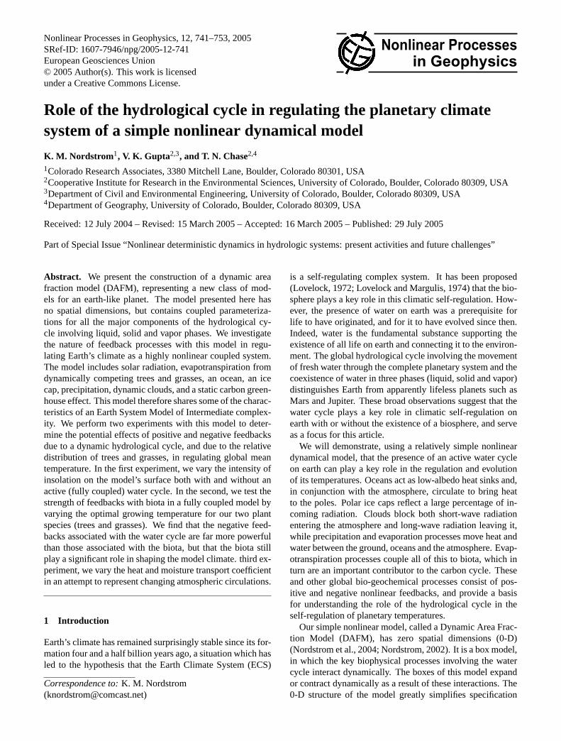
Fig. 1. Power law plot of rainfall and cloudiness over Beijing,China, 1951–1990. Data is from Wang et. al., 1993.
as soil moisture. However, because the size of the barefraction ad is not determined solely by the biota, includingother variables in the vegetation birth rate overdetermines themodel. In such a case, trees and grasses may not simultane-ously exist in steady state. We therefore elect to retain a birthrate dependent only on temperature.
2.4 Hydrological cycle
Water vapor is the largest greenhouse gas in the atmosphere.Therefore, the distribution of water in the atmosphere is im-portant for specification of radiative effects like cloud re-flectivity and greenhouse forcing. Functional relationshipsbetween surface water vapor characteristics and column in-tegrated water vapor have been tested with some success(Choudhoury, 1996). We therefore choose to keep track of agiven region’s mean precipitable water, denotedwi , as a sim-ple measure of region mean atmospheric water vapor. Massbalance gives
wi = Ei − Pi + Fwi + Kwi (14)
whereEi is evaporation,Pi is precipitation,Fwi representsthe interregional atmospheric moisture transport, andKwi
is the DAF adjustment for precipitable water. We use theMagnus-Tetens formulae for estimating thermodynamic vari-ables at saturation. Using the formula for saturation den-sity ρs(T ) for water vapor, we can calculate the saturationmass per unit area for a vertical column of atmosphere us-ing a linear temperature profile with lapse rateγl=6.5 K/m(Emanuel, 1994) with
wsat (Ti) =
∫ H
0ρs(Ti + γlz)dz. (15)
A measure of the total relative humidity for a column cannow be writtenri=wi/wsat (Ti).
PrecipitationPi is, of course, difficult to represent in a0-D model. Convective rainfall is highly variable in both
space and time, and to accurately represent this requires avery sophisticated parameterization. We elect, therefore, tosimply view precipitation as the mechanism by which the at-mosphere sheds excess water. As such, we leave a convec-tion parameterization for the future and keep track of onlyannual mean rainfall, which has units of mass over time.The timescale should depend inversely upon local saturation,since a highly saturated atmosphere will rain more quicklythan an unsaturated one. We therefore write
Pi = f ′ wi = (f rpi )wi, (16)
after the parameterization used byPaul(1996), which devel-oped annual rainfall proportional to precipitable water, butwith an additional power law dependence on column relativehumidity. Mean annual regional cloudiness correlates loga-rithmically to precipitation (Fig.1), so we take the regionalcloud area fraction to be
aci = acoPαi . (17)
The empirical parametersf , p, aco, andα are to be deter-mined from data.
Cloud albedoAci is a sensitive function of cloud height(Hobbs and Deepak, 1981), and we assume that clouds format a constant temperatureTc across our model. A linear pro-file for temperature, which we have already assumed for sat-uration, means thatHc(Ti)=(Ti−Tc)/γl and
Aci(Ti) = Aco + κHc(Ti). (18)
HereTc is the cloud top temperature from Eq. (3), 1γl
is thelinear slope for cloud height, andAco is the cloud albedo forclouds at the surface. The linear response of cloud albedo tocloud height,κ, is an empirical parameter to be determinedfrom data.
To represent evaporation, we choose a Penman-Monteithresistance model of the form
Ei =(Rin,i − Rout,i)φ(Ti) + ρacpa(esat (Ti) − ei)rh
(φ(Ti)rh + γh(rh + rsi))Lv
, (19)
whereρa is the density of the ambient air,cpa is the heatcapacity of the ambient air,rh is the hydrodynamic re-sistance of bare soil,γh is the “psychrometer constant”,and Lv is the latent heat of vaporization of liquid water.φ(Ti) is an estimate of the derivative of the saturation va-por pressureesat (Ti) close to the ground (Monteith, 1981),ei=eo[ln(mwi)+Tc]
ex is the vapor pressure determined fromthe column integrated moisture (Emanuel, 1994), andrsi isthe stomatal resistance of the region’s biota. Stomatal resis-tance is a function of many things, most sensitively ambientcarbon dioxide concentrations; but also intensity of sunlight,ambient temperature, and ambient relative humidity. Sincecarbon dioxide is fixed in this version of the model, in veg-etated regions we take resistance to be a function of relativehumidity
rsi = 1/(h1 + h2ri), (20)
K. M. Nordstrom et al.: Role of the hydrological cycle in regulating the planetary climate system 745
settingh1=.004 m/s andh2=.096 m/s for consistency withthe Ball-Berry model of stomatal conductance (Ball et al.,1987; Pleim, 1999). In non-vegetated regions,rsi=0.
The greenhouse forcing,ν, is taken to be a linear functionof moisture. Here
ν = νc + νwmwi, (21)
with νc the (constant) carbon forcing andνw the absorptivityof water across the visible and thermal spectra. Both param-eters remain to be estimated from data.
Soil moisture is also an important variable to track, sinceits distribution determines, to a large extent, the ability ofvegetation to survive. Mass balance for the soil gives us
ρwdsoil swi = (Pi − Ei + Fsi + Ksi), (22)
for si the soil water content in soildsoil deep; ρw is thedensity of water. We chooseFsi=Ds(s−si), andKsi anal-ogously toKT i . Therefore, we take the death rate for biotato be a quadratic function ofsi , the simplest function that iszero at both saturation and drought.
We will assume for the purposes of this model that all in-terregional atmospheric transports occur through bulk move-ment of air, and thus through atmospheric circulation pat-terns. Then moisture transports in the atmosphere will followthe movement of heat, and they should reduce when there aresmaller quantities of water in the atmosphere. We thereforemakeFwi proportional toFT i and the ratio of global meanprecipitable waterw to the mean precipitable water at thecurrent luminosity,w |L=1.0. This assumption yields
Fwi = [Dm(w
w |L=1.0)]FT i, (23)
in whichDm is a constant determined by matching moisturecontent over the model ice caps to present day polar valueswith w=w |L=1.0. The value forw |L=1.0 can be found fromPeixoto and Oort(1992) to be about 25.5 kg/m2.
2.5 Oceans
Oceans may be represented by a dynamic area fraction, withbirth rate proportional to precipitation and runoff, and withdeath rate proportional to evaporation. Thus,
ao = (ao[Po − Eo + Fso] + aabl µice)/Mo (24)
whereµice is melt from the ablation zone of the polar capsandMo is the mass of a column of ocean water. We assumea constant mean ocean depth for simplicity. Although theactual adjustment of the ocean fraction is small due to thelarge value of the constantMo, the effect of small changesin ao on the hydrological cycle in the rest of the model ispotentially significant.
The presence of the soil moisture convergence termFso,included to capture the effects of runoff from land processes,requires the specification of a preferred soil moisture for theocean, since we can’t directly write down a sensible analogof soil moisture in the ocean. Then
Fso = Ds(s − so), (25)
with so a constant to be determined.
2.6 Ice caps
Ice caps can also be represented as a dynamic area frac-tion, but the DAF must be divided into two regions, an ab-lation zone and an accumulation zone. The division betweenthese zones will be made by mean annual temperature, sinceannual snowmelt in the polar regions is principally deter-mined by temperature and not by solar radiation (Bowman,1982). We therefore construct a line of freezingθf rz, insideof which ice sheets tend to grow and outside of which theyablate. The ice sheet poleward ofθf rz, where no significantsnowmelt occurs, will be known as the “accumulation zone”;whereas the ice sheet towards the equator fromθf rz will bereferred to as the “ablation zone”. This parameterization isconstructed after the model discussed inGhil and Childress(1987).
The freezing line is demarcated by a mean annual tem-perature equal to an effective freezing temperature,Tf e, dis-cussed below.θf rz may then be determined from the globalradiative balance by noting that the solar constant varies si-nusoidally with co-latitude, and may be reasonably approxi-mated by a square root for easy invertability. If we approx-imate the solar luminositySθ=S(Aθ+Bθ
√(θ)), we can de-
termine a co-latitudeθ at which a given steady-state temper-atureTθ will occur by using a steady state assumption on (1),such that
θ = [(Rin(wθ , Tθ ) + FT ,θ )/Rout (wθ , Tθ ) − Aθ ]2/B2
θ . (26)
Herewθ is the local atmospheric moisture at temperatureTθ ,which can be found through a steady state assumption ona mass balance Eq. (14). Note thatKw,θ=0 becausewθ isassociated with a region of zero area.
The fractional area of a sphere that lies within a givenco-latitudeθ ′ is (1− cosθ ′)/2. If we assume north-southsymmetry, this is multiplied by a factor of two such that thefractional area of a globe with an annual mean temperaturelower thanTθ is aθ=1− cosθ . Hence, the accumulation zonehas areaaacc=1− cosθf rz, θf rz is the co-latitude at whichsnowmelt for the year is zero, and the ablation zone has areaaabl=ai−aacc.
Under the DAF formalism, the area of the ice sheet updateswith different precipitation- and evaporation-dependent massbalance rates in each subregion so that
ai = aacc(Pacc − Eacc)/MI + aabl(Pabl − Eabl − Nabl)/MI ,(27)
whereNabl is a melt rate andMI is the mean mass of a col-umn of ice. Note that this formulation assumes a square pro-file for the ice sheet for simplicity, though it is possible to as-sume other profiles, as well. Moisture and temperature vari-ables must be calculated for each subregion to closePacc,Eacc, Pabl , andEabl . These variables are computed fromtheir respective balances at the zonal center of each subre-gion.
DAF adjustment termsKHi become somewhat tricky overthe ice. This is in part because the accumulation zone ex-pands into the ablation zone rather than the bare land fraction
746 K. M. Nordstrom et al.: Role of the hydrological cycle in regulating the planetary climate system
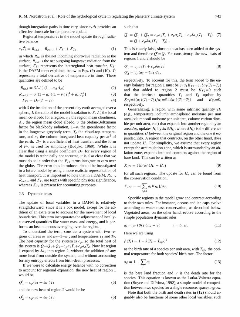
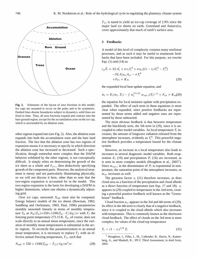
Fig. 2. Schematic of the layout of area fractions in this model.Ice caps are assumed to occur on the poles and to be symmetric.Dashed lines denote boundaries subject to dynamics, solid lines arefixed in time. Thus, all area fractions expand and contract into thebare ground region, except for the accumulation zone on the ice cap,which is surrounded by an ablation zone.
other regions expand into (see Fig.2). Also, the ablation zoneexpands into both the accumulation zone and the bare landfraction. The fact that the ablation zone has two regions ofexpansion means it is necessary to specify in which directionthe ablation zone has increased or decreased. Such a spec-ification, though somewhat more complex than the DAFMbehavior exhibited by the other regions, is not conceptuallydifficult. It simply relies on determining the growth of theice sheet as a whole andθf rz, then deductively specifyinggrowth of the component parts. However, the analytical treat-ment is messy and not particularly illuminating physically,so we will not discuss it here, other than to note that thetwo-region expansion is accounted for in the model. Thistwo-region expansion is the basis for developing a DAFM inhigher dimensions, where one obtains a dynamically adjust-ing grid.
Over ice caps, snowmeltNabl must also be computed.Energy balance models of the ice sheets (Bowman, 1982;Sandberg and Oerlemans, 1983; Paul, 1996) parameterizemonthly snowmelt linearly in terms of monthly tempera-tureTm asNm(Tm)=550+1100(Tm−Tf )kg/yr with Tf thefreezing point temperature 273.15 K.Tm, of course, does notscale directly to an annual mean temperature, since the vari-ation of monthly mean temperatures is substantial in the arc-tic regions. To reconcile this parameterization to an annualmean temperature, it is necessary to replaceTf with an ef-fective annual freezing temperature,Tf e such that
Nabl = 550+ 1100(Tabl − Tf e) kg/m2yr. (28)
Tf e is tuned to yield an ice-cap coverage of 2.9% since themajor land ice sheets on earth, Greenland and Antarctica,cover approximately that much of earth’s surface area.
3 Feedbacks
A model of this level of complexity contains many nonlinearprocesses, and as such it may be useful to enumerate feed-backs that have been included. For this purpose, we rewriteEqs. (1) and (14) as
cpTi = SLA′
i + σνiT4i + σaci[(1 − νi)T
4i − T 4
c ]
−SLA′
iaciAci − σT 4i
+FT i + KT i (29)
the expanded local heat update equation, and
wi = Ei(wi, Ti) − f w(1+p)i wsat,i(Ti)
−p+ Fwi + Kwi,(30)
the equation for local moisture update with precipitation ex-panded. The effect of each term in these equations is moreclear when expanded, since positive feedbacks are repre-sented by those terms added and negative ones are repre-sented by those subtracted.
The most obvious feedback is that between temperatureand the blackbody term, the 5th term in (29), since it is un-coupled to other model variables. As local temperatureTi in-creases, the amount of longwave radiation released from theatmosphere increases, evidently asT 4
i . This powerful nega-tive feedback provides a temperature bound for the climatesystem.
However, an increase in a local temperature also leads toincreases in several diagnostic model variables. Both evap-oration Ei (19) and precipitationPi (16) are increased, asis seen in more complex models (Houghton et al., 20051).Sincemsat,i in the denominator ofPi is exponential in tem-perature, the saturation point of the atmosphere increases, somwi increases as well.
The greyness factorνi (21) therefore increases, as doescloud area as a function of the precipitation and cloud albedoas a direct function of temperature (see Eqs.17 and18). νi
appears in (29) coupled to temperature in the 2nd term, creat-ing a powerful positive feedback well known as the “Green-house” feedback.
Cloud fractionaci appears in the 3rd and 4th terms of (29).Its effect in the 4th term is clearly that of a negative feedback,since it is coupled to the cloud albedo which also increaseswith temperature. This is commonly known as the shortwavecloud feedback. The effect of clouds on the 3rd term is morecomplex; for values of the cloud top temperature
Tc < (1 − νi)1/4 Ti (31)
1 Houghton, J., Filho, L. M., Callender, B., Harris, N., Katten-berg, A., and Maskell, K.: IPCC Third Assessment, in draft form,2005.
K. M. Nordstrom et al.: Role of the hydrological cycle in regulating the planetary climate system 747
Table 1. Major feedbacks included in the full model.
Feedback Effect Components involved
blackbody negative temperature, heatcloud albedo negative atmospheric moisture, temperaturebiota albedo negative plant fraction, temperaturegreenhouse positive atmospheric moisture,temperatureice albedo positive ice fraction,temperaturecloud longwave positiveTc<(1−νi)
1/4 Ti ; else, negative atmospheric moisture, temperature
this feedback will be positive, but forTc>(1−νi)1/4 Ti this
feedback is negative! That is, for high values of the grey-ness factor in this model, the effect of clouds in the longwavecan actually be to cool the planet, an interesting feedbackto be sure. However, it must be noted that such a situationis not physically realistic, since heat must first escape fromthe greenhouse gases below the clouds in order to reach theclouds and the model does not account for this. The possibil-ity of such a feedback is thus an artifact of our assumption ofa constant cloud top temperature. We can view relation (31)as providing an upper bound for estimation of the parameterTc in the model.
There is an ice-albedo feedback in the model, a positivefeedback produced by the high reflective capabilities of polarice. The accumulation angleθ (26) increases as a function ofFT ,θ , which increases asT decreases. Thus colder tempera-tures lead to a larger accumulation of ice, which reflects moreheat.
Other feedbacks come from the surface processes in themodel. From Eq. (11) with β(Ti) expanded andγ (si)=γo +
γ ′(si−sopt )2,
ai = aiad − aiadk(Ti − Topt )2− aiγ (32)
The second term in this equation is a biota albedo feedback,negative since it increases as the local temperature straysfrom the optimal.
Feedbacks with ocean fraction are negligible, since thepercent change of the area of the ocean system is extremelysmall. Major feedbacks in the model are listed in Table1.
4 Parameter Estimation
As with any model, the DAFM requires the specification ofseveral parameters and we choose these to resemble an earth-like climate. As a general and consistent rule, model param-eters are selected to bring the system variables to approxi-mately match annual means on earth. However, the parame-terizations themselves are applied by linearly scaling the an-nual mean estimates to the time scale of model integration,1/1000th of a year, and by varying them on that timescale.
Our representation of the hydrological cycle demandsspecification of a fallout frequency,f ; the relative humid-ity exponentp for precipitation; a base cloudiness,aco; the
precipitation exponent for cloudiness,α; the surface tem-perature slope for cloud albedo,κ; the minimum albedo forclouds,Aco; the greenhouse greyness due to carbon,νc; thewater vapor slope for water vapor greyness,νw; the preferredoceanic soil moisture,so; the coefficient for the linear trans-port of atmospheric moisture,Dw; the coefficient for the lin-ear transport of soil moisture,Ds ; the snowmelt temperature,Tf e; and the cloud top temperatureTc.
We use data taken over Beijing, China (Wang et al., 1993)to find our power law exponent,α=.1, indicating a weak de-pendence for cloudiness on precipitation (Fig.1). Since theearth’s mean cloudiness at our current temperature is 49%,we can findaco from the mean conditions. The mean surfacetemperature of the earth is around 288.4 K, its mean precip-itable water is about 25.5 kg/m2, and its mean albedo is 30–35% (Peixoto and Oort, 1992). The minimum cloud albedoAco, generally associated with low-lying fog, we take to be.05 to match the albedo of the ocean. For stability the modelrequiresκ≤1/60, and for largerκ the clouds become increas-ingly more capable of adjusting albedo to block solar input;thus we takeκ to be its minimum possible value to preventexcessive bias towards homeostatic behavior in the hydro-logical cycle. Then, from the earth’s mean albedo, we candetermine the cloud top temperatureTc.
Ice sheets cover 2.9% of the earth’s surface, which allowsus to determine the annual melting temperatureTf e. Theprecipitation exponentp, representing the power law depen-dence of precipitation frequency on column humidity, we de-termine by matching the frequency found from data in theice cap model ofPaul(1996) at earth-like conditions in ourparameterization. We can now determine the frequency co-efficientf from the mean column moisture on earth.
The moisture transport coefficient we assume to be con-stant over the globe by construction; its value can be esti-mated from the polar moisture transport listed inPeixoto andOort (1992). For simplicity, we useDw=Ds , dividing mois-ture flux evenly between atmosphere and land. Model behav-ior is relatively insensitive to variations in this parameter inthe neighborhood of its estimated value.
The carbon greynessνc is tuned to represent about 5% ofthe greenhouse forcing. For a soil composed of 10% sand and10% clay, saturation occurs atsi≈.45 and drought forsi≈.1(Salisbury and Ross, 1992). The ocean’s preferred soil mois-ture,so, is set to the midpoint of these two values,so=.275.

748 K. M. Nordstrom et al.: Role of the hydrological cycle in regulating the planetary climate system
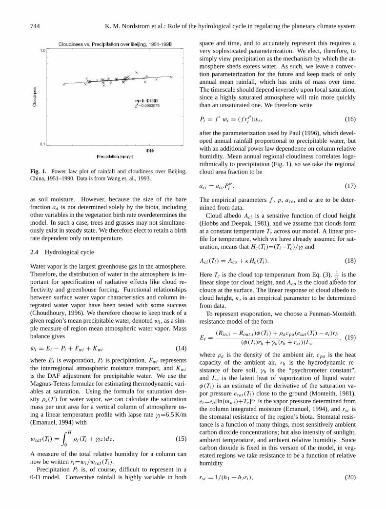
Fig. 3. Comparison of global mean temperatureT vs. luminosityL in a DAFM integration with fixed hydrological cycle to a DAFMwith a dynamic hydrological cycle. Biota is dynamic and identi-cally forced in both plots. The hydrological cycle in the full DAFMproduces an exceptionally strong stabilizing effect.
Taking a conservative estimate of the carbon greenhousegreyness, we can determineνw finally from the earth’s meantemperature. Values of parameters used in our model runsfor this analysis are listed in Tables2 and3.
5 Analysis
We perform two numerical experiments to emphasize the ef-fects of feedbacks between various components of the hydro-logical cycle on the global mean temperature of the model.In the first experiment, we compare runs of the fully coupledmodel with runs of a reduced model implementing only statichydrological variables over a range of solar luminositiesL.
In the second experiment, we modify theTopt parameter,the uniform optimal temperature for seedling growth of bothtrees and grasses in the model. In the real ECS, this parame-ter may vary from species to species, and is not well known ingeneral, so modifying the parameter serves two purposes: 1.,to test model sensitivity to an unknown value; and 2., to showthe range of control vegetation can have over surface temper-atures through changing evaporative properties and albedo.
As a basis for comparison in both experiments, we runthe model to a steady state for earthlike conditions, as de-fined by a modern solar luminosity (L=1), a mean temper-ature near 288.5 K, mean precipitable water near 25.5 K, anice cap fraction near 3%, cloudiness near 50%, realistic tem-peratures and precipitation near the poles, and approximatelyequal coverage for our two plant species.
5.1 Comparison to a fixed hydrological cycle varyingL
The intent of this experiment is to establish a qualitative ideaof the combined effects of various feedbacks between the hy-drological cycle and the heat balance on a planet like earth.
As such, we first compile data from a set of runs of the fullmodel with solar luminosities ranging from 70% of presentday insolation to 130%. In what follows, we shall refer tothis set with the labelε(L).
For the second set of runs, labelled8(L), we fix all vari-ables associated with the hydrological cycle in the model, in-cluding regional cloudiness, regional cloud albedo, ice frac-tion, regional precipitable water, ocean fraction, regional pre-cipitation, and regional evaporation, to the values obtained inthe earthlike run,ε(L=1). Like ε(L), this data set is obtainedby varyingL. Vegetation fractions and energy balances arethe only climate components in8(L) allowed to respond tochanges in insolation.
The contrast between the surface temperature values inthe full model and those in that without water feedbacks isstriking (Fig.3). Changes in the global mean temperature inε(L) are substantially smaller than they are in8(L), indicat-ing that an active hydrological cycle represents a tremendousnet negative feedback for all values ofL. This result is par-ticularly interesting in light of the fact that two very strongand extremely important positive hydrological feedbacks arepresent inε(L) but not in8(L), namely the ice-albedo andhydrological greenhouse feedbacks.
Since these are well-known to be positive feedbacks, otherhydrological quantities in the radiative balance must be re-sponsible for this behavior. The only ones remaining are thenonphysical longwave cloudiness effect and the shortwavecloud albedo effect, which represent two possible mecha-nisms for a stabilizing effect. The first is due to an increaseof both cloud area and cloud albedo in the shortwave termwith increasing temperatures, and the second is due to theincreased absorption and reemission of longwave radiationfrom the surface in the presence of more clouds. We wouldlike to show that the latter is not the cause of this behavior,since we have discussed earlier that it is not physically rele-vant.
In Fig. 4 we plot the incoming shortwave radiation at themodel’s surface over the five regional surface types. The im-portant feature in this plot is that the surfacial insolation onthree of the four upper regional curves vary from their meanson the order of 5% or less over the entire range of values ofL tested. The only exceptions are the region of bare ground,which varies on the order of 7%, and the ice cap, which cov-ers a very small fraction of the surface. This range ofL repre-sents a variation of 30% from its mean, so the behavior of theshortwave to solar forcing is extremely stable. It should alsobe noted that the slopes of these lines are generally decreas-ing with L. From Eq. (1) and the fact that the model residesat steady state, we can loosely approximate this behavior asa constant. Then we can write
Rin,i = Rout,i − FT i, (33)
in which all temperature dependence resides on the right sideand the left side is approximately a regionally dependent con-stant,Ri . Summing over regions to eliminate the transport
K. M. Nordstrom et al.: Role of the hydrological cycle in regulating the planetary climate system 749
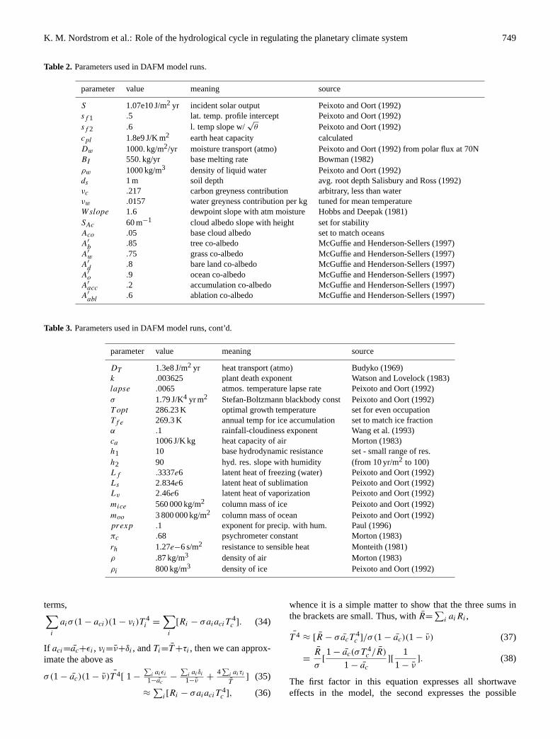
Table 2. Parameters used in DAFM model runs.
parameter value meaning source
S 1.07e10 J/m2 yr incident solar output Peixoto and Oort(1992)sf 1 .5 lat. temp. profile intercept Peixoto and Oort(1992)sf 2 .6 l. temp slope w/
√θ Peixoto and Oort(1992)
cpl 1.8e9 J/K m2 earth heat capacity calculatedDw 1000. kg/m2/yr moisture transport (atmo) Peixoto and Oort(1992) from polar flux at 70NBI 550. kg/yr base melting rate Bowman(1982)ρw 1000 kg/m3 density of liquid water Peixoto and Oort(1992)ds 1 m soil depth avg. root depthSalisbury and Ross(1992)νc .217 carbon greyness contribution arbitrary, less than waterνw .0157 water greyness contribution per kg tuned for mean temperatureWslope 1.6 dewpoint slope with atm moisture Hobbs and Deepak(1981)SAc 60 m−1 cloud albedo slope with height set for stabilityAco .05 base cloud albedo set to match oceansA′
b.85 tree co-albedo McGuffie and Henderson-Sellers(1997)
A′w .75 grass co-albedo McGuffie and Henderson-Sellers(1997)
A′d
.8 bare land co-albedo McGuffie and Henderson-Sellers(1997)A′
o .9 ocean co-albedo McGuffie and Henderson-Sellers(1997)A′
acc .2 accumulation co-albedo McGuffie and Henderson-Sellers(1997)A′
abl.6 ablation co-albedo McGuffie and Henderson-Sellers(1997)
Table 3. Parameters used in DAFM model runs, cont’d.
parameter value meaning source
DT 1.3e8 J/m2 yr heat transport (atmo) Budyko(1969)k .003625 plant death exponent Watson and Lovelock(1983)lapse .0065 atmos. temperature lapse rate Peixoto and Oort(1992)σ 1.79 J/K4 yr m2 Stefan-Boltzmann blackbody constPeixoto and Oort(1992)T opt 286.23 K optimal growth temperature set for even occupationTf e 269.3 K annual temp for ice accumulation set to match ice fractionα .1 rainfall-cloudiness exponent Wang et al.(1993)ca 1006 J/K kg heat capacity of air Morton (1983)h1 10 base hydrodynamic resistance set - small range of res.h2 90 hyd. res. slope with humidity (from 10 yr/m2 to 100)Lf .3337e6 latent heat of freezing (water) Peixoto and Oort(1992)Ls 2.834e6 latent heat of sublimation Peixoto and Oort(1992)Lv 2.46e6 latent heat of vaporization Peixoto and Oort(1992)mice 560 000 kg/m2 column mass of ice Peixoto and Oort(1992)moo 3 800 000 kg/m2 column mass of ocean Peixoto and Oort(1992)prexp .1 exponent for precip. with hum. Paul(1996)πc .68 psychrometer constant Morton (1983)rh 1.27e−6 s/m2 resistance to sensible heat Monteith(1981)ρ .87 kg/m3 density of air Morton (1983)ρi 800 kg/m3 density of ice Peixoto and Oort(1992)
terms,∑i
aiσ(1 − aci)(1 − νi)T4i =
∑i
[Ri − σaiaciT4c ]. (34)
If aci=ac+εi , νi=ν+δi , andTi=T +τi , then we can approx-imate the above as
σ(1 − ac)(1 − ν)T 4[ 1 −
∑i aiεi
1−ac−
∑i aiδi
1−ν+
4∑
i aiτi
T] (35)
≈∑
i[Ri − σaiaciT4c ], (36)
whence it is a simple matter to show that the three sums inthe brackets are small. Thus, withR=
∑i aiRi ,
T 4 ≈ [R − σ acT4c ]/σ(1 − ac)(1 − ν) (37)
=R
σ[1 − ac(σT 4
c /R)
1 − ac
][1
1 − ν]. (38)
The first factor in this equation expresses all shortwaveeffects in the model, the second expresses the possible
750 K. M. Nordstrom et al.: Role of the hydrological cycle in regulating the planetary climate system
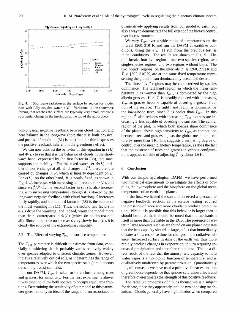
Fig. 4. Shortwave radiation at the surface by region for modelruns with fully coupled water,ε(L). Variations in the shortwaveforcing that reaches the surface are typically very small, despite asubstantial change in the insolation at the top of the atmosphere.
non-physical negative feedback between cloud fraction andheat balance in the longwave (note that it is both physicaland positive if condition (31) is met), and the third expressesthe positive feedback inherent in the greenhouse effect.
We can now contrast the behavior of this equation inε(L)
and8(L) to see that it is the behavior of clouds in the short-wave band, expressed by the first factor in (38), that mostsupports the stability. For the fixed-water set8(L), nei-ther ac nor ν change at all; all changes inT 4, therefore, arecaused by changes inR, which is linearly dependent onL.For ε(L), on the other hand,R is nearly fixed, as shown inFig.4. ac increases with increasing temperature forε(L), andsinceσT 4
c /R<1, the second factor in (38) is also increas-ing with increasing temperature (though it is slowed by thelongwave negative feedback with cloud fraction).ν increasesfairly rapidly, and so the third factor in (38) is the source ofthe most warming inε(L). Thus, the second two factors inε(L) drive the warming; and indeed, warm the model morethan their counterparts in8(L) (which do not increase atall). Since the first factor increases very slowly forε(L), it isclearly the source of the extraordinary stability.
5.2 The Effect of varyingTopt on surface temperatures
The Topt parameter is difficult to estimate from data, espe-cially considering that it probably varies relatively widelyover species adapted to different climatic zones. However,it plays a relatively critical role, as it determines the range oftemperatures over which the two species state (simultaneoustrees and grasses) can exist.
In our DAFM, Topt is taken to be uniform among treesand grasses, for simplicity. For the first experiments above,it was tuned to allow both species to occupy equal area frac-tions. Determining the sensitivity of our model to this param-eter gives not only an idea of the range of error associated in
quantitatively applying results from our model to earth, butalso a way to demonstrate the full extent of the biota’s controlover its environment.
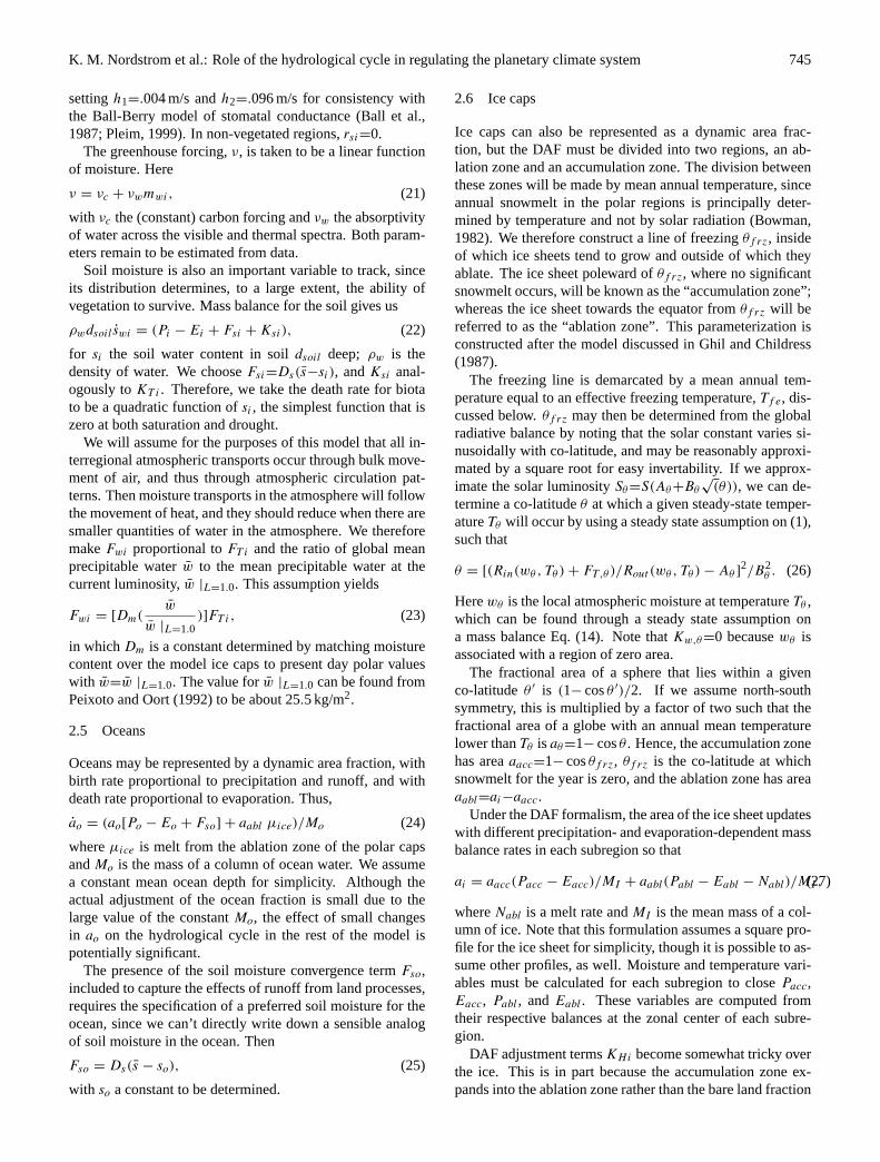
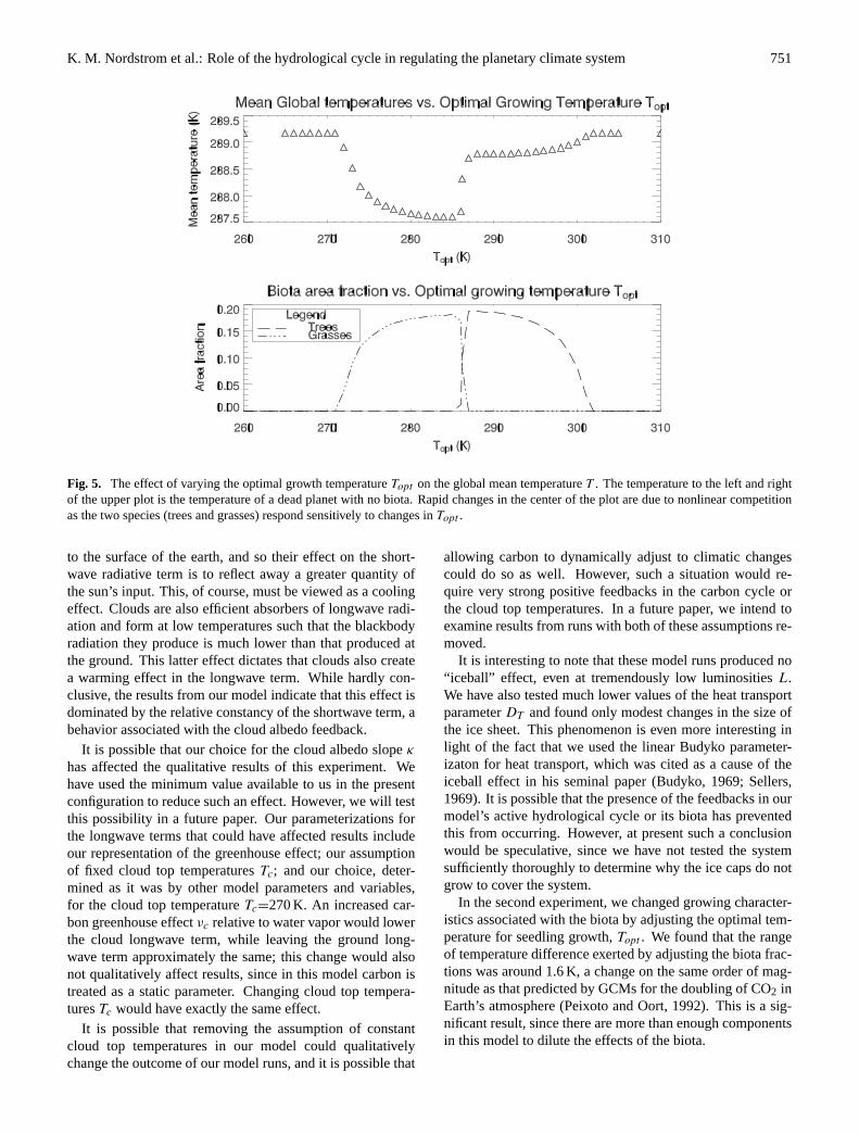
We vary Topt over a wide range of temperatures on theinterval [260, 310] K and run the DAFM at earthlike con-ditions, using theε(L=1) run from the previous test asinitial conditions. The results are shown in Fig.5. Theplot breaks into five regions: one two-species region, twosingle-species regions, and two regions without biota. Thetwo “dead” regions, on the intervalsT ∈ [260, 271] K andT ∈ [302, 310] K, are at the same fixed temperature repre-senting the global mean dominated by ocean and desert.
The three “live” regions may be characterized by speciesdominance. The left hand region, in which the mean tem-peratureT is warmer thanTopt , is dominated by the highalbedo grasses. HereT is steadily reduced with increasingTopt as grasses become capable of covering a greater frac-tion of the surface. The right hand region is dominated bythe low-albedo trees, sinceT is cooler thanTopt . In thisregion, T also reduces with increasingTopt as trees are in-creasingly less capable of covering the surface. The centralregion of the plot, in which both species share dominanceof the planet, shows high sensitivity toTopt , as competitionbetween trees and grasses adjusts the global mean tempera-ture by more than 1 K. This suggests a surprising degree ofcontrol over the mean planetary temperature, as does the factthat the existence of trees and grasses in various configura-tions appears capable of adjustingT by about 1.6 K.
6 Conclusion
With our simple hydrological DAFM, we have performedtwo numerical experiments to investigate the effects of cou-pling the hydrosphere and the biosphere on the global meantemperature of an earth-like planet.
In the first, we heated the sun and observed a spectacularnegative feedback reaction, as the surface heating requiredthe presence of more and more clouds to produce precipita-tion. While it is possible that this behavior is larger than itshould be on earth, it should be noted that the mechanismitself is more than plausible in the ECS. The presence of wa-ter in large amounts such as are found on our planet indicatesthat the heat capacity should be large, a fact that immediatelydictates a slow response time for changes in the radiative bal-ance. Increased surface heating of the earth will thus morerapidly produce changes in evaporation, in turn requiring in-creased precipitation and therefore cloudiness. This is a di-rect result of the fact that the atmospheric capacity to holdwater vapor is a monotonic function of temperature, and isqualitatively unaffected by parameterization. Quantitativelyit is, of course, as we have used a primitive linear estimationof greenhouse dependence that ignores saturation effects andtherefore overestimates the strength of this positive feedback.
The radiative properties of clouds themselves is a subjectfor debate, since they apparently include two opposing mech-anisms. Clouds generally have high albedos when compared
K. M. Nordstrom et al.: Role of the hydrological cycle in regulating the planetary climate system 751
Fig. 5. The effect of varying the optimal growth temperatureTopt on the global mean temperatureT . The temperature to the left and rightof the upper plot is the temperature of a dead planet with no biota. Rapid changes in the center of the plot are due to nonlinear competitionas the two species (trees and grasses) respond sensitively to changes inTopt .
to the surface of the earth, and so their effect on the short-wave radiative term is to reflect away a greater quantity ofthe sun’s input. This, of course, must be viewed as a coolingeffect. Clouds are also efficient absorbers of longwave radi-ation and form at low temperatures such that the blackbodyradiation they produce is much lower than that produced atthe ground. This latter effect dictates that clouds also createa warming effect in the longwave term. While hardly con-clusive, the results from our model indicate that this effect isdominated by the relative constancy of the shortwave term, abehavior associated with the cloud albedo feedback.
It is possible that our choice for the cloud albedo slopeκ
has affected the qualitative results of this experiment. Wehave used the minimum value available to us in the presentconfiguration to reduce such an effect. However, we will testthis possibility in a future paper. Our parameterizations forthe longwave terms that could have affected results includeour representation of the greenhouse effect; our assumptionof fixed cloud top temperaturesTc; and our choice, deter-mined as it was by other model parameters and variables,for the cloud top temperatureTc=270 K. An increased car-bon greenhouse effectνc relative to water vapor would lowerthe cloud longwave term, while leaving the ground long-wave term approximately the same; this change would alsonot qualitatively affect results, since in this model carbon istreated as a static parameter. Changing cloud top tempera-turesTc would have exactly the same effect.
It is possible that removing the assumption of constantcloud top temperatures in our model could qualitativelychange the outcome of our model runs, and it is possible that
allowing carbon to dynamically adjust to climatic changescould do so as well. However, such a situation would re-quire very strong positive feedbacks in the carbon cycle orthe cloud top temperatures. In a future paper, we intend toexamine results from runs with both of these assumptions re-moved.
It is interesting to note that these model runs produced no“iceball” effect, even at tremendously low luminositiesL.We have also tested much lower values of the heat transportparameterDT and found only modest changes in the size ofthe ice sheet. This phenomenon is even more interesting inlight of the fact that we used the linear Budyko parameter-izaton for heat transport, which was cited as a cause of theiceball effect in his seminal paper (Budyko, 1969; Sellers,1969). It is possible that the presence of the feedbacks in ourmodel’s active hydrological cycle or its biota has preventedthis from occurring. However, at present such a conclusionwould be speculative, since we have not tested the systemsufficiently thoroughly to determine why the ice caps do notgrow to cover the system.
In the second experiment, we changed growing character-istics associated with the biota by adjusting the optimal tem-perature for seedling growth,Topt . We found that the rangeof temperature difference exerted by adjusting the biota frac-tions was around 1.6 K, a change on the same order of mag-nitude as that predicted by GCMs for the doubling of CO2 inEarth’s atmosphere (Peixoto and Oort, 1992). This is a sig-nificant result, since there are more than enough componentsin this model to dilute the effects of the biota.
752 K. M. Nordstrom et al.: Role of the hydrological cycle in regulating the planetary climate system
It remains to add dynamic carbon feedbacks to this model,like those studied inSvirezhev and von Bloh(1998). A futurepaper coupling the two cycles would certainly produce inter-esting results. It would likewise be interesting to establish lo-cal heat capacities,cpi . In addition, more spatial dependencyshould be added, as biota have different growing character-istics at different latitudes and the effect of landform loca-tion is suspected of playing some role in determining globalclimate. Using different optimal growing temperatures fortrees and grasses might also allow us to include growth de-pendence on other model variables, such as soil moisture.
More generally, there is a great need in this and other mod-els to develop a rigorous framework for parameterizations,one that explicitly incorporates the basic issue of scale de-pendence and scale invariance in biophysical processes. Forexample, in this model and others (Pan, 1990), a Penman-Monteith equation has been used to represent evapotranspi-ration at relatively large spatial scales. However,Choudury(1999) found that the Penman-Monteith equation was notscale invariant across a very broad range of spatial scalestested in the biophysical model they studied. Such a re-sult reinforces that the Penman-Monteith equation is validonly for very specific scales and should not be directly ap-plied to larger ones. At present, the study of scaling trans-formations on biophysical parameterizations is in its infancy(e.g.Milne et al.(2002)). Thus the biophysical parameteriza-tions available to modelers at present are typically not scale-appropriate.
Finally, there is a need to establish model parameteriza-tions in all climate models consistent with some establishedset of basic physical principles. Unfortunately, there has beenrelatively little attention paid to how to elucidate such a setof principles in a system like Earth’s climate system, whichis a highly nonlinear system far from equilibrium or steadystate. For example, a promising candidate in this area is theMaximal Entropy Production (MEP) formalism developedby Paltridge(1975) and others (for an excellent review seeOzawa et al.(2003)). Only by establishing such a consis-tent theoretical framework will we be able to effectively de-velop parameterizations capable of representing higher-ordermoments as well as the means, or ensure consistency in ourphysical schemes and the results. In future DAFM modelswe intend to explore the development of parameterizationsunder a MEP formalism.
Acknowledgements.The first author would like to thank theNational Science Foundation (NSF) for its generous supportunder a Graduate Research Traineeship (GRT) grant awarded tothe University of Colorado hydrology program, which made thedevelopment of this work possible as part of his PhD disserta-tion. He and the second author would also like to acknowledgeNSF for its continued support as the work evolved under grantsEAR-9903125 and EAR-0233676.The third author wishes toacknowledge NSF grant number ATM-0001476 in support ofthis research. All the three authors gratefully acknowledge theCIRES Innovative Research Program for its support of this research.
Edited by: B. SivakumarReviewed by: two referees
References
Ball, J., Woodrow, I., and Berry, J.: A model predicting stomatalconductance and its contribution to the control of photosynthesisunder different environmental conditions, Progress in Photosyn-thesis Research, IV, 221–234, 1987.
Bowman, K.: Sensitivity of an annual mean diffusive energy bal-ance model with an ice sheet, J. Geophys. Res., 87, 9667–9674,1982.
Boyce, W. and DiPrima, R.: Elementary differential equations andboundary value problems, 5th ed., Wiley, New York, 1992.
Budyko, M.: The effect of solar radiation variations on the climateof the Earth, Tellus, 5(9), 611–619, 1969.
Choudhoury, B.: Comparison of two models relating precipitablewater to surface humidity using globally distributed radiosondedata over land surfaces, Int. J. Climatol., 16, 663–675, 1996.
Choudury, B.: Evaluation of an empirical equation for annual evap-oration using field observations and results from a biophysicalmodel, J. Hydrol., 216, 99–110, 1999.
Claussen, M., Crucifix, M., Fichefet, T., Ganopolski, A., Goosse,H., Lohmann, G., Loutre, M.-F., Lunkeit, F., Mohkov, I., Mysak,L., Petoukhov, V., Stocker, T., Stone, P., Wang, Z., Weaver, A.,and Weber, S.: Earth system models of intermediate complexity:Closing the gap in the spectrum of climate system models, Clim.Dyn., 18, 579–586, 2002.
Emanuel, K.: Atmospheric convection., Oxford Univ. Press, NewYork, 1994.
Ghil, M. and Childress, S.: Topics in geophysical fluid dynamics:Atmospheric dynamics, dynamo theory, and climate dynamics,Springer-Verlag, NY, 1987.
Harvey, L. and Schneider, S.: Sensitivity of internally generated cli-mate oscillations to ocean model formulation, in: Proceedings onthe Symposium on Milankovitch and Climate, edited by: Berger,A., Imbrie, J., Hays, J., Kukla, S., and Saltzman, B., ASI, pp.653–667, NATO, D. Reidel, Hingham, MA, 1987.
Hobbs, P. and Deepak, A.: Clouds: Their formation, optical prop-erties, and effects, Academic Press, NY, 1981.
Houghton, J., Filho, L. M., Callender, B., Harris, N., Kattenberg,A., and Maskell, K.: Contribution of working group I to the sec-ond assessment of the intergovenmental panel on climate change,in: IPCC Second Assessment – Climate Change 1995, MITPress, Cambridge, MA, 1995.
Lovelock, J.: Gaia as seen through the atmosphere, Atmos. Envi-ron., 6, 579–580, 1972.
Lovelock, J. and Margulis, L.: Atmospheric homeostasis by and forthe biosphere: the Gaia hypothesis, Tellus, 26, 1–10, 1974.
McGuffie, K. and Henderson-Sellers, A.: A climate modelingprimer (Research and development in climate and climatology),J. Wiley and Sons, NY, 1997.
Milne, B., Gupta, V., and Restrepo, C.: A scale invariant couplingof plants, water, energy, and terrain, Ecoscience, 9(2), 191–199,2002.
Monteith, J.: Evaporation and surface temperatures, Quarterly Jour-nal of the Royal Meteorological Society, 107, 1–27, 1981.
Morton, F.: Operational estimates of areal evapotranspiration andtheir significance to the science and practice of Hydrology, J.Hydrol., 66, 1–76, 1983.
K. M. Nordstrom et al.: Role of the hydrological cycle in regulating the planetary climate system 753
Nordstrom, K.: Simple models for use in Hydroclimatology, Ph.D.thesis, University of Colorado at Boulder, 2002.
Nordstrom, K., Gupta, V., and Chase, T.: Salvaging the Daisyworldparable under the Dynamic Area Fraction Framework, in: Scien-tists Debate Gaia: the next century, edited by: Miller, J., Boston,P., Schneider, S., and Crist, E., MIT Press, Cambridge, MA,2004.
O’Brian, D. and Stephens, G.: Entropy and climate II: Simple mod-els, Quarterly Journal of the Royal Meteorological Society, 121,1773–1796, 1995.
Ozawa, H., Ohmura, A., Lorenz, R., and Pujol, T.: The secondlaw of thermodynamics and the global climate system: a reviewof the maximum entropy production principle, Rev. Geophys.,41(4), 1018, 2003.
Paltridge, G.: Global dynamics and climate – A system of minimumentropy exchange, Quart. J. Roy. Meteor. Soc., 101, 475–484,1975.
Pan, H.-L.: A simple parameterization scheme of evapotranspi-ration over land for the NMC medium-range forecast model,Monthly Weather Review, 118, 2500–2512, 1990.
Paul, A.: A seasonal energy balance climate model for coupling toice-sheet models, Ann. Glaciol., 23, 174–180, 1996.
Peixoto, J. and Oort, A.: Physics of climate, American Institue ofPhysics, NY, 1992.
Pleim, J.: Modeling stomatal response to atmospheric humidity, inPreprints of the 13th Symposium on Boundary Layers and Tur-bulence, January 10–15 1999 in Dallas, TX, American Meteoro-logical Society, Boston,MA, 1999.
Salisbury, F. and Ross, C.: Plant physiology (4th ed.), WadsworthPublishing Co., Belmont, CA, 1992.
Sandberg, J. and Oerlemans, J.: Modelling of Pleistocene Europeanice sheets: The effect of upslope precipitation, Geologie en Mjin-bouw, 62, 267–273, 1983.
Sellers, W.: A global climatic model based on the energy balanceof the Earth-atmosphere system, J. Appl. Meteorol., 8, 392–400,1969.
Svirezhev, Y. M. and von Bloh, W.: Climate, vegetation, and globalcarbon cycle: the simplest zero-dimensional model, EcologicalModeling, 101, 79–95, 1998.
Wang, W., Zhang, Q., Easterling, D., and Karl, T.: Beijing cloudi-ness since 1875, J. Clim., 6, 1921–1927, 1993.
Watson, A. and Lovelock, J.: Biological homeostasis of the globalenvironment: the parable of Daisyworld, Tellus, 35B, 284–289,1983.
Weber, S.: On homeostasis in Daisyworld, Climatic Change, 48,465–485, 2001.


![arXiv:1001.5285v3 [physics.soc-ph] 4 Oct 2011 · Boston University, ... 2Cooperative Association for Internet Data Analysis (CAIDA), University of California-San ... Stern School](https://static.fdocuments.us/doc/165x107/5b8eb14509d3f2b01e8b66e0/arxiv10015285v3-4-oct-2011-boston-university-2cooperative-association.jpg)


![Student Evaluation in Cooperative Learning · 2012-11-03 · Cooperative Learning 3 Student Evaluation in Cooperative Learning: 1 Teacher Cognitions 2Cooperative Learning [CL] demands](https://static.fdocuments.us/doc/165x107/5f9737e9c435ee4e9b39b813/student-evaluation-in-cooperative-learning-2012-11-03-cooperative-learning-3-student.jpg)


