Role of Somatosensory and Vestibular Cues in Attenuating Visually Induced

Human Postural Sway

/

Robert J. Peterka, Ph.D. and Martha S. Benolken, B.A.

Legacy Good Samaritan Hospital & Medical Center, Clinical Vestibular Laboratory

and R.S. Dow Neurological Sciences Institute, Portland, OR 97210, USA

Send correspondence to:

Robert J. Peterka

Legacy Good Samaritan Hospital1040 NW 22nd Avenue, N010

Portland, OR 97210

(503)229-8154

(503)274-4944 fax

peterka@nsi.lhs.org

(NASA-CR-197845) ROLE OF

SOMATOSENSORY AND VESTIBULAR CUES

IN ATTENUATING VISUALLY INOUCED

HUMAN POSTURAL SWAY (Legacy Good

SaMaritan Hospital) 32 p

G3/53

N95-27697

Unclas

0049948

https://ntrs.nasa.gov/search.jsp?R=19950021276 2018-11-12T03:50:19+00:00Z

Abstract

The purpose of this study was to determine the contribution of visual,

vestibular, and somatosensory cues to the maintenance of stance in humans.

Postural sway was induced by full field, sinusoidal visual surround rotations about

an axis at the level of the ankle joints. The influences of vestibular andsomatosensory cues were characterized by comparing postural sway in normal and

bilateral vestibular absent subjects in conditions that provided either accurate or

inaccurate somatosensory orientation information.

In normal subjects, the amplitude of visually induced sway reached a saturation

level as stimulus amplitude increased. The saturation amplitude decreased with

increasing stimulus frequency. No saturation phenomena was observed in subjects

with vestibular loss, implying that vestibular cues were responsible for the

saturation phenomenon. For visually induced sways below the saturation level, thestimulus-response curves for both normal and vestibular loss subjects were nearly

identical implying that (1) normal subjects were not using vestibular information toattenuate their visually induced sway, possibly because sway was below a

vestibular-related threshold level, and (2) vestibular loss subjects did not utilize

visual cues to a greater extent than normal subjects; that is, a fundamental change

in visual system "gain" was not used to compensate for a vestibular deficit.

An unexpected finding was that the amplitude of body sway induced by visual

surround motion could be almost three times greater than the amplitude of thevisual stimulus in normals and vestibular loss subjects. This occurred in conditions

where somatosensory cues were inaccurate and at low stimulus amplitudes. A

control system model of visually induced postural sway was developed to explain

this finding.For both subject groups, the amplitude ofvisuaUy induced sway was smaller by

a factor of about four in tests where somatosensory cues provided accurate versus

inaccurate orientation information. This implied that (1) the vestibular loss

subjects did not utilize somatosensory cues to a greater extent than normal subjects;that is, changes in somatosensory system "gain" were not used to compensate for a

vestibular deficit, and (2) the threshold for the use of vestibular cues in normals was

apparently lower in test conditions where somatosensory cues were providingaccurate orientation information.

Key Words: postural control -- vestibular -- somatosensory -- vision -- human

Introduction

Moving visual scenes have long been known to induce postural adjustments inhuman subjects (Berthoz et al. 1979; Brandt et al. 1986). A wide variety of moving

visual stimuli have been employed to investigate this phenomenon including tilting

rooms (lateral and fore-aft rotations about an axis at the level of the ankle joints

(Bles et al. 1983; Bles et al. 1980)), swinging rooms (Lee and Lishman 1975),projected displays simulating a moving visual wall (van Asten et al. 1988), tunnel,

floor, or ceiling (Lestienne et al. 1977; Soechting and Berthoz 1979), and visual roll

rotations (Clement et al. 1985; Dichgans et al. 1972).

Direct comparisons among studies are difficult because a variety of visual

stimuli have been employed and differing techniques have been used for measuring

2

body motion. Most experiments have shown that postural adjustments were in thedirection of the visual field motion (Berthoz et al. 1979; Bles et al. 1983; Bles et al.1980; Clement et al. 1985; Dichgans et al. 1972; Lestienne et al. 1977), butoppositely directed body sways have also been reported in some subjects (van Astenet al. 1988). One consistent finding has been the existence of a saturation effect;that is, increases in the amplitude of the visual field movement cause little or noadditional postural sway (Bles et al. 1980; Clement et al. 1985; Lestienne et al.1977; van Asten et al. 1988). Below the saturation level, postural sway deviationshave been shown to be proportional to the logarithm of the visual motion amplitude(Lestienne et al. 1977). The stimulus amplitude at which saturation occursapparently depends upon the availability of accurate somatosensory and vestibularorientation cues. Standing on a compliant surface (foam), which decreases ordisrupts somatosensory cues, increases the amplitude of visually induced sway atsaturation (Bles et al. 1980). Patients with loss of somatosensation due topolyneuropathy also show increased responsiveness to visual motion (Kotaka et al.1986). In addition, loss of vestibular function results in increased responsiveness tovisual motion stimuli in comparison to normal subjects, although this effect isfrequency dependent (Bles et al. 1983).

The purpose of this study was to clarify the role of vestibular and somatosensoryinformation in human postural control by comparing visually induced sway innormal subjects and bilateral vestibular loss patients standing in environmentswith and without reliable somatosensory cues. This work addressed three specificquestions. First, is the increased susceptibility of vestibular loss patients to visuallyinduced sway caused by an increase in visual drive to postural control or due to aloss of attenuation of visually induced sway normally provided by the vestibularsystem? Second, does a comparison of visually induced sway in normals andvestibular loss subjects reveal the presence of vestibular-related thresholdproperties in normals? Third, is there evidence for enhanced utilization ofsomatosensory and/or visual information in order to compensate for a loss ofvestibular function?

A portion of these results were previously published in a conference proceedings(Peterka and Benolken 1992).

Materials and methods

The experimental protocols described here were approved by the Institutional

Review Board of Legacy Health System and were performed in accordance with the1964 Helsinki Declaration. All subjects gave their informed consent prior to

entering the study. We tested 9 subjects ranging in age from 22 to 67 years. Six

subjects (aged 22--45) had normal clinical sensory organization tests of posturalcontrol (Peterka and Black 1990) and no history of balance or dizziness complaints.

Three subjects (aged 50--67) had bilateral vestibular losses; two were judged to havea profound bilateral loss by the absence of a vestibulo-ocular reflex on rotation tests

and severe vestibular dysfunction pattern on sensory organization tests of posturalcontrol (Peterka and Black 1990), and 1 had a severe, but not total bilateral loss as

judged by a greatly reduced vestibulo-ocular reflex on rotation tests and severe

vestibular dysfunction pattern on sensory organization tests. Although the normal

and vestibular loss subjects differed in age, control trial measures showed noindication of a difference between the normal and vestibular loss groups in their

3

utilization of visual and somatosensory cues for balance control. Sensoryorganization test results for vestibular loss subjects were well within normal limitson test conditions which did not require vestibular cues for balance. Previous workcharacterizing age-related changes in postural control have identified only minorchanges with age in a subject's ability to utilize visual and somatosensory cues(Peterka and Black 1990).

Subjects were tested on a modified Equitest (NeuroCom, Clackamas, OR)moving posture platform. The visual surround on the posture platform rotatedunder servo control about an axis which was collinear with the ankle joint axis andwas located about 10 cm above and 16 cm forward of the ankle joint position. Thevisual surround was modified to provide a visually provocative scene. The surfaceof the visual surround facing the subject was located about 65 cm from the subject'seyes and consisted of a circular target pattern of concentric 6.5 cm wide rings ofalternating black and white sectors. This pattern was similar to the pattern W2 ofvan Asten et al. (1988). The right and left sides of the visual surround were located47 cm from midline and consisted of a checkerboard pattern of alternating back andwhite rectangles 6.3 by 20.3 cm. Tests were performed in a darkened room with thevisual surround illuminated by a fluorescent light attached to the visual surroundto keep the illumination level constant as the visual surround moved. Subjects wereinstructed to maintain upright stance with as little sway as possible. White noisewas played into headphones to limit auditory cues to visual surround motion.However, we were not able to fully mask auditory and vibration cues during thelargest visual surround motions.

Subject anterior-posterior (AP) sway angle was measured by two horizontal rodsattached to the subject at the hip and shoulder level. One end of each rod wasattached to the subject and the other end to an earth-fixed potentiometer. The APdisplacements of the subject's body at the level of the hips and shoulders werecalculated using the output of the two potentiometers with appropriatetrigonometric conversions. These measures were used to estimate the body center-of-gravity (CG) displacement using a two part body model which assumed thesubject had an average distribution of body mass between the upper and lower bodysections (Peterka and Black 1990). The motion of the body was expressed as theangular rotation (in degrees) of the CG point about the ankle joint axis with apositive sign indicating a forward body sway.

Thirty-six tests over three test sessions were performed by each subject. Half ofthe tests were performed with the subject standing on a fixed support surface, andhalf on a sway-referenced support surface (seeexplanation of sway-referencingbelow). Two tests were control trials performed with eyes open and with no motionof the visual surround. In thirty-four tests the visual surround was sinusoidallyrotated at 3 different frequencies (0.1, 0.2 or 0.5 Hz) and 6 different amplitudes(peak displacement amplitudes of 0.2°, 0.5°, 1°, 2°, 5° or 10°). All combinations offrequencies and amplitudes were given except 10° at 0.5 Hz due to motorlimitations. The initial motion of the visual surround was always away from thesubject. The test sequence was random. An integer number of stimulus cycleswaspresented over a 60 s duration with a 1 s baseline recorded prior to the start of thestimulus. If a subject fell on a test, that test was immediately repeated up to twomore times. Stimulus delivery and data sampling were computer controlled at aclock rate of 50/s. Sampled data included visual surround and support surface

4

rotational positions, vertical forces exerted on the support surface, and body swayangles at the level of the hip and shoulder.

Sway-referencing was performed by rotating the posture platform's supportsurface (rotation axis through the ankle joints) in direct proportion to the subject'slower body sway angle as measured by the sway rod attached at the subject's hip.Sway-referencing maintains the ankle joint angle nearly constant over time(assuming no knee flexion). This reduces the contribution of somatosensory cuesassociated with ankle joint motions which are normally well correlated with bodysway when a subject is standing on a fixed surface. The extent to which sway-referencing reduces somatosensory cues is uncertain. However it is certain that thereduction was sufficient to eliminate a vestibular loss subject's ability to maintainupright stance when no other sensory orientation cueswere available. This wasdemonstrated by the consistent falls exhibited by the vestibular loss subjectsattempting to stand with eyesclosed on a sway-referenced surface. The nature ofthe falls indicated that no corrective responses were generated, and thereforesuggested that somatosensory cueswere greatly reduced. In contrast, vestibularloss subjects were able to maintain stance with eyesclosed on a fixed supportsurface. Sway-referencing was initiated at the start of sinusoidal visual surroundmotion.

The CG sway angle time series was used for the analysis of the steady stateresponses to the visual stimulus. A Fourier analysis of the steady state CG swayangle and the visual surround angle time series was used to calculate the amplitudeof CG sway, amplitude of visual surround motion, and phase of CG sway relative tothe stimulus motion. Fourier transforms of the CG sway angle and visual surroundangle time series were calculated using the following formulas:

2 ¢.N (2xfi_ 2 _ . (2Xfi'_

O_(f) = F{0o_(i)} = c-_ _=_00g(i) cos|_/\ r ]- J_ 2_0¢s(i)c.N ___ sm_--_--)

[1]

e_(O = y{e,(i)} [2]

where e_(i) is the sampled CG time series, 0v(i) is the sampled visual surround

angle time series, j = _Z_, c is the number of stimulus cycles analyzed, N is the

number of sample points per stimulus cycle, r is the sampling rate, and f is the

frequency (in Hz) at which the Fourier transform was calculated, ec_(f) and 0v(f) are

complex quantities. The amplitude of CG sway and of visual surround motion at a

frequency, f, was given by:

]Ocs(f) = 4Re[0¢g(f)]2 + Im[0¢g(f)] 2 [3]

Io.,(o= 4Re[0_(f)]2 + Im[e.,,(f)] 2 [4]

The transfer function, H(f), between the visual stimulus and the CG body sway was

calculated by:

5

H(_- eogff) [5]e,(19

The gain and phase of the transfer function were given by:

IH(igl = _Re[H(f)] 2 + Im[H(f)] 2 [6]

_,(Im[H(f)]

ZH(f) = tan [ /Re[H(f)] d[7]

The first cycle of the CG and visual surround time series were not included in the

Fourier analysis in order to avoid transient responses. Since most of this study'sresults were concerned with the CG sway response to the visual stimulus motion,

the Fourier analysis was performed at the frequency of the visual stimulus motion.

In some cases I ecg(f) I was calculated over a range of frequencies to determine the

overall spectrum of CG sway (see Figure 2).

Fourier analysis was also performed on spontaneous CG sway data (eyes openwith no visual surround motion) under both fixed and sway-referenced support

surface conditions. The spectral amplitudes, I 0_(f) I, of spontaneous sway at 0.1,

0.2, and 0.5 Hz provided control data for comparison with visually induced sway

amplitudes.

Calculations of sway amplitudes and gains using Fourier techniques are

potentially biased due to the presence of noise (Bendat and Piersol 1971; Otnes and

Enochson 1972). Extensive simulation studies were performed in order todetermine if major bias errors were a likely source of error in the calculation of

response amplitudes and gains at the stimulus frequency. Using the Fourier

analysis methods described above, simulation results showed that bias errors in the

measurement of response amplitude were minimal for noise levels that resembled

those seen in the experimental data. Bias errors were below 10% of the trueresponse amplitude for noise amplitudes up to 50% of the true response amplitude.

Various alternative windowing techniques, cross-spectral analysis methods, andFourier analysis using segmented data sets were used to determine if biases could

be reduced by alternative analysis methods (Otnes and Enochson 1972). None of

the alternatives gave lower biases than the analysis used in this study.

Results

The visual surround motion induced a steady state CG sway response at the

stimulus frequency and in the same direction as the visual surround motion. Figure1 shows CG sways induced by the 0.2 Hz, 1° peak amplitude visual surround motion

with a sway-referenced support surface. In most traces, a clear response at the

stimulus frequency can be seen although response amplitudes varied, particularly

among the normal subjects. Figure 2 shows amplitude spectra of CG sway for both

normal and vestibular loss subjects during a 0.2 Hz, 1 o sinusoidal visual surround

rotation. Spectra of CG sway in both sway-referenced (data from Figure 1) and

fixed support surface conditions are shown. In addition, amplitude spectra of

control trials (eyes open with fixed visual surround) are shown for comparison. A

6

Fourier analysis (eqns. [1] and [3]) was used to compute the amplitude spectra overa frequency range of 0.05 to 1 Hz.

Y1_il $SmL_= (_ I _)

01

_mo (=!

I.0_ i

0.

E

0.5

_ 0.0

Fixed Condition Sway-referenced Condition2.0-

1.S o

1.0.

Ii 0.5.

..... , ..... =.,, 0.0 ...... , ...... _-"._i0.1 1 0.1 1

Frequency (Hz)

Fig 1. Representative CG sway time series of 3

vestibular loss and 6 normal subjects during 60

s visual surround rotations at 0.2 Hz frequency

and 1 ° peak amplitude with a sway-referencedsupport surface. Upward deflection represents

rotation of the visual surround away from the

subject and forward body sway.

Fig. 2. Example amplitude spectra of CG sway

from vestibular loss and normal subjects. The

amplitude spectra shown were computed by

taking the average of individual test spectraobtained from each subject's CG sway data.

Average spectra from the 3 vestibular loss

subjects are shown as dashed lines and average

spectra from the 6 normals as solid lines. Thick

lines indicate spectra from control tests and thin

lines indicate spectra from the 0.2 Hz, 1 ° visualsurround motion tests. Amplitude spectra under

both fixed support surface conditions (left) and

sway-referenced conditions (right) are shown withdifferent scales on the ordinate axes.

The control trial spectra in Figure 2 show that normal and vestibular loss

subjects had similar amplitudes and frequency distributions of CG sway. The

spectral component of CG sway at the 0.2 Hz visual stimulus frequency was

enhanced compared to the control trial amplitude at this frequency. At this specificstimulus frequency and amplitude, the visual surround motion induced about twice

the CG sway amplitde in vestibular loss subjects as compared to the normalsubjects in the sway-referenced condition, and about 2.5 times the sway in the fixedcondition.

In the remainder of the results section, we are concerned only with the Fourier

component of sway which is at the stimulus frequency. When we refer to the

response amplitude, we are referring to the Fourier component amplitude computed

from eqn [3] with f equal to the stimulus frequency.

Fixed Condition

4j 0.1 HZ -e-.VestbulaJ'Lo_ |

to. z,,t _ '

OI _..-; -0- ....... _ = .......

0.5 Hz +

2 5 10

SwRf.referenced Condition

4 IO.1

2 ,.

o/#,'t i o.2

0:_-;

410.5

.z : ; ;:2 •

o.%-,o12 0.5_ 2 g 1o

VisuaJ Surround Amplitude (deg)

Fig. 3. CG sway amplitude measured at the visual stimulus

frequency as a function of visual surround stimulus amplitudeunder fixed (left column) and sway-referenced (right column)

conditions at three frequencies of visual surround motion.

The +'s indicate the number of vestibular loss subjects who

fell during a given trial. The small dots (7 points) represent

the individual data from vestibular loss subjects who did not

fall on a particular trial in which others did fall. Six of seven

of the individual points, including the 2 lowest amplitude

points in the 0.5 Hz fixed condition, are from the vestibular

loss subject with the greatest preservation of vestibularfunction. Data points plotted with error bars (mean + 1

standard error) are data from normal subjects (open squares)

or data from vestibular loss subjects (large solid dots) where

all subjects completed a given trial. Data plotted at zerostimulus amplitude are the control trial spontaneous CG sway

amplitudes determined by Fourier analysis at the respective

frequencies and support surface conditions. Dashed lines

show the average amplitude of saturated sway in the normal

subjects.

The amplitude of visually

induced sway in normal and

vestibular loss subjects wasdependent upon stimulus

frequency, stimulus

amplitude, and the support

surface condition. Figure 3

shows the amplitude of CGsway as a function of thevisual surround stimulus

amplitude for different

stimulus frequencies andsupport surface conditions. Inboth normal and vestibular

loss subjects, visual surround

motion induced larger

amplitude sways in sway-

referenced as compared to

fixed support surface

conditions at any givenstimulus amplitude and

frequency.Normal subjects did not

fall on any trial with fixed

support surface conditions.Occasional falls occurred

among normals during sway-referenced trials, but the

normal subjects were always

able to complete the trials

upon repetition of the test

condition. Some of the largeramplitude visual surroundmotions caused consistent falls

in vestibular loss subjects.

Vestibular loss subjects fell in

both fixed and sway-

referenced support surface conditions, with falls occurring at lower stimulus

amplitudes when the support surface was sway-referenced. The vestibular losssubject with some preservation of vestibular function (the severe vestibular loss

subject) was more resistant to falling than the two subjects with no evidence of

vestibular function (profound vestibular losses). The severe vestibular loss subject's

resistance to falls was more evident on the fixed support surface trials. Specifically,on 0.1 Hz, 10 °, and 0.2 Hz, 5 ° and 10 ° fixed support surface trials, his visually

induced sway was about six times larger than the average of the normal subjects.

However his performance on the 0.5 Hz, 2 ° and 5 ° trials was close to the average

response of normal subjects. His normal performance at the highest test frequency

is consistent with observations that higher frequency vestibular responses are

8

preserved relative to lower frequency function in subjects with severe vestibularlosses (Honrubia et al. 1985).

Saturation and threshold phenomena

Among normal subjects tested under sway-referenced conditions (Figure 3, rightcolumn), a saturation in the amplitude of visually induced CG sway occurred as the

visual stimulus amplitude increased (most evident in the 0.1 Hz sway-referenceddata). The saturation level decreased with increasing stimulus frequency. Below

the saturation level, CG sway increased in proportion to the logarithm of the visual

stimulus amplitude. For the vestibular loss subjects there was no saturation effect.

That is, visually induced sway increased as a function of the logarithm of the

stimulus amplitude until falls occurred at higher stimulus amplitudes.

For sway-referenced test conditions which evoked responses with amplitudesbelow the saturation levels, the amplitude of visually induced sway was similar in

normal and vestibular loss subjects up to the point where the normal subjects

reached the saturation level. Specifically, the 0.1 Hz sway-referenced data showed

similar amplitudes of induced sways in normals and vestibular loss subjects for

stimulus amplitudes of 0.2 °, 0.5 °, and 1% but a clear divergence between normalsand vestibular loss subjects at stimulus amplitudes of 2 ° and above (falls occurred

in vestibular loss subjects with 5 ° and 10 ° stimuli). At 0.2 Hz, the induced sways

were nearly identical for normals and vestibular loss subjects only at the lowest

stimulus amplitude of 0.2 °, with a clear divergence between the test groups at

higher stimulus amplitudes. At 0.5 Hz, visually induced sway in vestibular losssubjects was greater than in normal subjects even at the lowest stimulus amplitude

of 0.2 °.

Visually induced sway under fixed support surface conditions (Figure 3, lei_column) showed a similar pattern of frequency and amplitude dependence as in the

sway-referenced condition. However, under fixed support surface conditions the

amplitudes of visually induced sway were about four times lower than incorresponding sway-referenced conditions. As in the sway-referenced condition,there was a saturation effect in the normal group at higher stimulus amplitudes.

For stimuli above the saturation level at any given frequency, there was a clear

divergence between the normal and vestibular loss groups in the amplitude ofvisually induced sway. The vestibular loss group showed increasing sway with

increasing stimulus amplitude (with falls occurring at higher stimulus amplitudes).Below the saturation levels, the induced sways were similar in the two groups.

This saturation phenomenon and the correspondence between the sway

amplitudes in normal and vestibular loss subjects at low stimulus amplitudes

suggests that normal subjects were not making use of vestibular motion cues atthese low sway amplitudes. That is, at sways below a threshold amplitude, normal

subjects did not attenuate visually induced sway more than vestibular loss subjects.These vestibular-related threshold amplitudes were estimated by averaging the CG

sway amplitudes at high stimulus amplitudes where the sway versus stimulus

amplitude curves for normal subjects diverged from those of the vestibular loss

subjects and saturated. The choice of which stimulus amplitude points to include in

these averages was based on visual inspection of the various curves. In each of thefixed condition tests the data from the highest 4 stimulus amplitudes were included

in the average. In the sway-referenced condition tests the 3, 5, and 4 highest

9

stimulus amplitude data at 0.1, 0.2, and 0.5 Hz, respectively, were included in theaverage. These threshold amplitudes are given in Table 1 and plotted as dottedlines in Figure 3. The threshold amplitudes decreased with increasing stimulusfrequency in both fixed and sway-referenced conditions. Under fixed supportsurface conditions, the threshold estimates were 3--5 times lower than under sway-referenced support surface conditions.

Table L Threshold estimates (saturated CG sway amplitude) in normal subjects (mean ± SE)

Fixed Condition Sway-referenced Condition

Frequency (Hz) Angular position (deg) Angular velocity (°/s) Angular position (deg) Angular velocity (°/s)

0.1 0.32 ± 0.06 0.20 ± 0.04 1.57 ± 0.15 0.99 + 0.09

0.2 0.17 ± 0.02 0.21 ± 0.03 0.98 + 0.11 1.23 ± 0.14

0,5 0.10 ± 0.02 0.31 ± 0.06 0.29 ± 0.04 0.92 ± 0.11

Response gain and phase.

c-

(.9

0

4

0.1 Hz •"_'-NorrnalFixed•-_-Notrnal Sway-ref

• .t-Ve61ibular k_. Fixed

la/loss Sway-mr

i . "":":'0":-:::

0.2Hz

00.1

0.5Hz

0.2 0.5 1 2 5 10

Visual Surround Amplitude (deg)

Fig. 4. Mean gain (ratio of CG sway

amplitude at the stimulus frequency to

visual surround stimulus amplitude) of

visually induced CG sway as a function

of visual surround amplitude at three

frequencies of visual surround motion.

Visually induced postural responses can

also be expressed in terms of response gain and

phase (eqns [6] and [7]). In fixed supportsurface test conditions, the gains for bothnormal and vestibular loss subjects were less

than unity at all stimulus amplitudes and

frequencies tested (Figure 4). At a givenstimulus frequency, gains of both normal and

vestibular loss subjects generally decreased

with increasing stimulus amplitude. Because

of the saturation phenomenon seen in normal

subjects, the gains of normals decreased more

rapidly with increasing stimulus amplitudethan did the gains of vestibular loss subjects.

In sway-referenced support surface test

conditions, the response gains of vestibular loss

subjects were greater than unity at all testfrequencies and amplitudes where data were

obtained. The gains were greatest at the lowesttest amplitude of 0.2 ° where the average gains

were 2.4, 2.9, and 2.6 at frequencies 0.1, 0.2,

and 0.5 Hz, respectively. Normal subjects also

had gains greater than or equal to unity at the

lowest test amplitude of 0.2 ° (average gains of1.9, 2.8, and 1.0 at frequencies 0.1, 0.2, and 0.5

Hz, respectively). The average gains of normals

were less than unity at stimulus amplitudes

greater than or equal to 2°,1 °,and 0.5° at 0.I,

0.2, and 0.5 Hz, respectively.

The phase of the CG sway angle relative to

the stimulus angular position is summarized in Table 2. Phase data were averaged

over all completed trials of a given test frequency and condition. The data show twogeneral trends. First, phases for both normal and vestibular loss subjects decreased

10

(increased phase lag) with increasing stimulus frequency. Second, at any givenfrequency and support surface condition, the average phase of vestibular losssubjects was advanced relative to the average phase of normal subjects.

Table 2. Phase of CG sway relative to visual surround position (degrees, mean + SE)

Fixed Condition Sway-referenced Condition

Frequency (Hz) Normal Vestibular Loss Normal Vestibular Loss

0.1 -12 + 16 21 :t: 6 19 + 11 41 + 5

0.2 -28 + 23 0 + 6 -30 + 13 11 :t: 11

0.5 -37 + 32 -16 + 17 -87 + 17 -81 + 15

The averaging of phase over all stimulus amplitude trials was justified at most

test frequencies and conditions since phase did not vary systematically with

stimulus amplitude. However there were exceptions. Specifically, the phases ofnormal subjects in 0.1 Hz and 0.2 Hz sway-referenced conditions and in 0.1 Hz fixed

conditions showed significant trends (P<0.05) of decreasing phase with increasing

stimulus amplitude. The trends were approximately proportional to the logarithm

of the stimulus amplitude. In all three of these data sets, the phase of the normalsubjects at the 0.2 ° test amplitude was closest to, but lagged the vestibular loss

subjects' phase. At higher stimulus amplitudes, the normal and vestibular loss

subjects' phases diverged since the vestibular loss subjects' phase remained

constant while the normal subjects' phase decreased.

The only test condition which showed a significant phase trend in the vestibularloss subjects was the 0.5 Hz sway-referenced condition. This trend was for

increasing phase with increasing stimulus amplitude. However this data set was

limited to only the lowest stimulus amplitudes since falls consistently occurred atthe higher amplitudes.

Dependence upon somatosensory cues

A comparison of subject performance under fixed versus sway-referenced

conditions provided information on the extent to which the availability of accuratesomatosensory cues decreased visually induced sway. This comparison was

quantified by computing the ratio of visually induced sway amplitude under fixedsupport surface conditions to the sway amplitude under sway-referenced conditions

in normal and vestibular loss subjects. The ratio was computed using only the

amplitude component of sway at the stimulus frequency. This ratio did not show

any trend with stimulus frequency or amplitude, and was nearly identical for thenormal and vestibular loss groups. The average ratio for normals over all test

conditions was 0.24 + 0.18 (mean _+1 SD) and for vestibular loss subjects was 0.24 _+

0.14. That is, a decrease in the accuracy of somatosensory cues caused adegradation of postural stability by the same factor for both normal and vestibular

loss subjects. This suggested that the vestibular loss subjects had not become more

reliant upon somatosensory cues (i.e. had not increased somatosensory gain) tocompensate for their vestibular loss.

11

Discussion

High gains of visually induced sway

The existence of gains greater than unity for visually induced sway was an

unexpected finding. These high gain responses occurred in both normal and

vestibular loss subjects under conditions where somatesensory orientation cueswere inaccurate (sway-referenced support surface conditions) and at low amplitudes

of visual surround motion. We are not aware of any description of high gains of

visually induced sway in previous studies. This is likely due to the fact that most

studies used larger amplitude visual surround motions which evoked proportionally

lower amplitudes of body sway (this is consistent with our data at higher stimulus

amplitudes). In addition, many studies used center-of-pressure energy measureswhich do not permit a calculation of sway gains. However one study (Lee and

Lishman 1975) showed an example figure of sway velocity and visual surround

stimulus velocity for a subject standing on a thick foam pad and exposed to a low

amplitude, 0.25 Hz sinusoidal AP oscillations of a visual surround. Although thestimulus was a linear translational visual surround movement, for comparison

purposes this movement would correspond to about a 0.1 o visual surround tilt

amplitude about the ankle joints. The induced sway velocity was clearly greater

than the stimulus velocity with an estimated gain of about 1.5.

CorrectiveAnkle

0 v Torque

_J Ko½ _qev- 0cg :_ e._,, 1 0cg,..

.L.I I -| T,rne KdS• Linearized

Delay Controller InVeBn¢_l__lndeUllum

Fig. 5. Simple linearized postural control system model of CG body sway, 0cg, induced by

visual surround motion, 0v. The model assumes that somatosensory and vestibular cues are

not contributing to body stabilization. Various model parameters are defined in the

discussion section (eqn [8]).

Consideration of the simplest possible model of postural control gives some

validity to the existence of high gains during visual motion stimulation. The control

system model in Figure 5 models the human body as an inverted pendulum. Themodel assumes there is no contribution of either somatosensory or vestibular motion

cues to the feedback control of the inverted pendulum. The body sway angle

relative to the visual surround angle (0v--0cg) is detected by the visual system with a

time delay of 0.2 seconds (visual processing and transmission delays). A corrective

torque about the ankle joint must be applied to maintain stability, and this

corrective torque is a function of 0v--0cg. In order for this system to be stable, it is

known (Johansson et al. 1988; Johansson, 1993) that the function of 0_--0cg must

include at least two terms; one proportional to 0_--0cg and one proportional to the

time derivative of 0_--0_g. With these two terms present, the overall transfer

function of this model is given by:

12

_ (Kds IS]O_(s) js 2 + (Kas + Kp)e-_' - mgh

where s is the Laplace transform variable, J is the moment of inertia of the body

about the ankle joint, m is the mass of the body, h is the height of the body's center-

of-gravity, g is acceleration due to gravity, Zd is a time delay, Kp is the

proportionality constant of 0v--0cg, and Ka is the proportionality constant of the time

derivative of 0v--0cg. J and mgh values of 62 kg-m 2 and 540 kg-m2/s 2, respectively,are reasonable estimates for subjects in this study (average mass 64 kg). The

predicted DC gain of this system (at s = 0) is equal to Kp/(Kp - mgh) and is therefore

greater than unity. Furthermore, only a limited range of Kp and Ka values, areconsistent with a stable system. The values Kp and Ka at the midpoint of their

stable ranges are 830 N-m/rad and 345 N-m-s/rad, respectively. With these values,the model predicts a DC gain of 2.9. In addition, the transfer function gain is nearly

constant at up to a frequency of 0.4 Hz. Above 0.4 Hz, the gain rises slowly to a

weak resonant peak at about 0.8 Hz and then declines.

The predicted transfer function gain values are reasonably consistent with the

gains observed in vestibular loss subjects at low stimulus amplitudes in the sway-referenced condition at all test frequencies. The predicted gains are also similar to

the low stimulus amplitude gains ofnormals at 0.1 and 0.2 Hz in the sway-referenced condition, but not at 0.5 Hz. This discrepancy at 0.5 Hz suggests that

the simple model in Figure 5, which assumes no somatosensory or vestibular

feedback, does not accurately represent the system at this test frequency. There is

no reason to expect that the somatosensory cues differ between the vestibular loss

and normal subjects at 0.5 Hz. However if a vestibular-related threshold

phenomena were present and the threshold level decreased with increasingfrequency, then vestibular motion information could contribute to postural

stabilization in normal subjects during a 0.5 Hz low amplitude stimulus, but not

during a 0.1 and 0.2 Hz low amplitude stimulus (see further discussion below).

Saturation and attenuation phenomena

CG sways of normal subjects induced by visual surround motion showed

nonlinear stimulus-response relations and saturation phenomenon such that

increasing amplitudes of visual surround motion did not evoke increasing CG sway.

In subjects with bilaterally absent vestibular function, this saturation phenomenonwas completely absent. In these vestibular loss subjects, increasing visual surround

motion induced increasing CG sways, resulting in consistent falls at larger stimulusamplitudes even when accurate somatosensory orientation cues were present (fixed

support surface conditions). This implies that the sensory cues which cause this

saturation phenomenon are of vestibular origin.The vestibular contribution to the attenuation of visually induced sway was

very different from the somatosensory contribution. For both normal and vestibularloss subjects, the availability of accurate somatosensory cues (fixed support surface

conditions) resulted in a fourfold decrease in visually induced sway gains in

comparison to test conditions with inaccurate somatosensory cues (sway-referenced

conditions). This somatosensory-related attenuation of gain Was independent of the

13

stimulus amplitude and frequency, and occurred in both normal and vestibular losssubjects. In contrast, the saturation phenomenon associated with the availability ofvestibular cues showed specific changes as a function of the stimulus frequency andamplitude (the saturation sway amplitude decreased with increasing frequency).

A saturation phenomenon has different functional consequencesthan a simplegain attenuation. If a subject is exposedto an environment with inaccurate visualorientation cues, the availability of an additional sensory orientation cue whichdecreasesvisually induced sway gain can decrease the likelihood of a fall, butcannot prevent a loss of balance. That is, a large amplitude visual motion stimuluscan always overcome the decreased gain. In contrast, a saturation effect cancompletely prevent a loss of balance independent of the visual stimulus amplitudeas long as the CG sway amplitude at saturation is within the normal stance range.

Threshold phenomenon

A comparison of the visually induced sway amplitude in normal and vestibular

loss subjects showed that the induced sway in normals and vestibular loss subjects

was similar until some critical, or threshold level of CG sway was reached. This

implies that normal subjects were not making use of vestibular motion information

to attenuate visually induced sway until some threshold CG sway amplitude wasexceeded.

Since head motions were not measured in these experiments, the observed

threshold phenomenon cannot be directly attributed to the vestibular system alone.

Studies have shown that head orientation in space tends to be stabilized during

various locomotor tasks (Grossman et al. 1988; Pozzo et al. 1990). Therefore the angular

or linear head motion components sensed by the vestibular system could be reduced

and altered compared to head motions predicted from CG sway measures which

assume that the head is rigidly fixed to the body. If there were changes in head

position with respect to the trunk during sway, then the observed threshold effects

might be related to an interplay between proprioceptive head motion informationfrom cervical afferents and vestibular motion information.

Mergner and coworkers (1991) hypothesized that, in some cases, information

from vestibular and neck proprioceptive systems used for motion perception is

combined and processed through the same central thresholding neural circuitry asis vestibular motion information alone. If the postural control system uses similar

mechanisms for processing combined vestibular and proprioceptive information,

then it is possible that the threshold properties derived from our visually induced

sway measures might be similar to vestibular thresholds identified by others usingpsychophysical measures.

In both fixed and sway-referenced support surface conditions, peak angular

position threshold amplitudes declined with increasing frequency. When thesethreshold measures were expressed in terms of angular velocity, their values were

approximately equal at the three test frequencies for a given support surface

condition (average amplitude of 1.05°/s or 2.1°/s peak-to-peak in the sway-

referenced condition, Table 1). This value is close to psychophysically derivedrotational motion thresholds (Benson et al. 1989; Benson and Brown 1992; Mergner

et al. 1991) which, when expressed in terms of angular velocity, are also relatively

constant over the range of test frequencies used in this study (0.1--0.5 Hz).

14

Under fixed support surface conditions, there was an apparent fourfold

reduction in threshold amplitudes (average amplitude of 0.24°/s or 0.48°/s peak-to-

peak in the fixed condition, Table 1) relative to the sway-referenced condition. Thisfourfold reduction could be analogous to the observation that angular motion

perception thresholds were lower by a factor of about three in experimentalsituations which evoked the oculogyral illusion in comparison to perceptual

thresholds measured in complete darkness (Benson and Brown 1989, 1992; Clark

and Stewart 1968). Another possible analogous situation, identified by Mergner

and coworkers (1991, 1993), is a task dependent change in threshold amplitudes

associated with the processing of neck and leg proprioceptive information for the

perception of relative movement of various body segments.What is the cause of the fourfold threshold shift associated with different

support surface conditions? One could speculate that the central postural system

actively adjusts thresholds to optimize balance control under varying environmentalconditions. For example, when visual and somatosensory orientation cues are

absent or inaccurate, it may be advantageous to have increased thresholds in orderto avoid vestibular-initiated control actions caused by small imbalances or

asymmetries of peripheral vestibular function. When other accurate sensory

orientation cues are present, these other cues might serve as a reference for

vestibular signals so that vestibular-initiated control actions could occur at lowerlevels of body sway. Alternatively, the apparent vestibular threshold shii_s might

be due to changes in the signal-to-noise ratio of vestibular signals. For example,

head movements associated with spontaneous body sway and due to the inherent

instability of the head-neck system (Goldberg 1992) would generate a baseline levelof "vestibular noise". In situations where accurate sensory orientation cues were

available from the visual and somatosensory systems, head stability in space would

be improved and therefore vestibular noise reduced. If postural responses were

evoked only when a vestibular signal rose above the baseline noise level, then

postural responses due to vestibular stimulation would be observed at lowerstimulus levels in low vestibular noise conditions (i.e. when accurate visual and

somatosensory cues were present) compared to high vestibular noise conditions.

Other evidence of threshold effects in postural control have recently beenobserved. Collins and De Luca (1993) analyzed center-of-pressure time series data

recorded during quiet stance. Their results suggested that short term postural

fluctuations were not controlled by closed-loop mechanisms until some systematicthreshold was exceeded. The existence of a threshold for the use of vestibular

information might contribute to the open-loop/closed-loop control strategy identifiedby Collins and De Luca.

Compensation for Vestibular Loss

One might expect that well-compensated vestibular loss subjects would adjustto their vestibular loss by altering the way in which somatosensory and/or visual

cues are used for postural control. That is, the appropriate strategy for using

somatosensory and visual sensory information for balance control might be differentwhen vestibular cues are not available, and central mechanisms might adapt to

achieve a more optimal utilization of the available visual and somatosensory

sensory cues.

15

Bles et al. (1983) tracked visually induced lateral body tilts over time in onepatient following a bilateral loss of vestibular function. The results generallyshowed decreases in the amplitude of induced sway over time which suggested thatsomatosensory cues were becoming more effective in attenuating the visuallyinduced sway. However the attenuation was frequency dependent with the greatestattenuation changes over time occurring at the lowest test frequency (0.025 Hz),and no attenuation occurring at the highest (0.2 Hz). Our test frequenciescorresponded to the upper range of frequencies used by Bles et al. (1983). At thesehigher frequencies we also were not able to identify compensatory changes in theuse of somatosensory cues in vestibular loss subjects.

If vestibular loss subjects compensated by increasing their sensitivity tosomatosensory cues for balance control, then the loss of somatosensory cuesor adecrease in accuracy of those cues should have a proportionally larger effect on theirbalance than it does on normal subjects. Our data showed that this was not thecase since both normal and vestibular loss subjects had nearly identical factor offour reductions of sway in the fixed versus the sway-referenced condition. Thissuggests that the vestibular loss subjects have not experienced a change insensitivity to somatosensory cues as a result of their loss of vestibular function overthe frequency range tested. As mentioned above, Bles et al. (1983) identifiedcompensatory changes at lower test frequencies and in more dynamic settings (Bleset al. 1984).

If one were to compare the sway amplitudes in normal and vestibular losssubjects during larger amplitude visual motion stimuli, one might conclude thatvisual motion sensitivity was increased in vestibular loss subjects. This increasedsensitivity might be the result of central compensatory adjustments for the loss ofvestibular function. However the data in Figure 3 indicate that low amplitudevisual surround movements induced approximately equal CG sway amplitudes inboth normals and vestibular loss subjects. This close correspondence between thelevels of induced sway in normal and vestibular loss subjects at low stimulusamplitudes suggests that the apparent increase in visual sensitivity in vestibularloss subjects is likely due to the absenceof vestibular suppression ofpostural swayrather than to a fundamental increase in sensitivity to visual motion.

Acknowledgments. This study was supported by NASA grants NAG 9-117 andNAGW-3782.

16

References

Bendat JS, Piersol AG (1971) Random data: Analysis and measurement procedures.

John Wiley & Sons, New YorkBenson AJ, Brown SF (1989) Visual display lowers detection threshold of angular,

but not linear, whole-body motion stimuli. Aviat Space Environ Med 60:629--633

Benson AJ, Brown SF (1992) Perception of liminal and supraliminal whole-body

angular motion. In: Berthoz A, GrafW, Vidal PP (eds) The head-neck sensory

motor system. Oxford University Press, New York, pp 483--487Benson AJ, Hutt ECB, Brown SF (1989) Thresholds for the perception of whole body

angular movement about a vertical axis. Aviat Space Environ Med 60:205--213Berthoz A, Lacour M, Soechting JF, Vidal PP (1979) The role of vision in the control

of posture during linear motion. Prog Brain Res 50:197--210

Bles W, Kapteyn TS, Brandt T, Arnold F (1980) The mechanism of physiological

height vertigo II. Posturography. Acta Otolaryngol (Stockh) 89:534--540

Bles W, de Jong JMBV, de Wit G (1983) Compensation for labyrinthine defects

examined by use of a tilting room. Acta Otelaryngol (Stockh) 95:576--579Bles W, de Jong JMBV, de Wit G (1984) Somatosensory compensation for loss of

labyrinthine function. Acta Otolaryngol (Stockh) 97:213--221

Brandt T, Paulus W, Straube A (1986) Vision and posture. In: Bles W, Brandt T

(eds) Disorders of posture and gait. Elsevier Science Publishers B.V., New York,

pp 157--175

Clark B, Stewart JD (1968) Comparison of sensitivity for the perception of bodilyrotation and the oculogyral illusion. Perception & Psychophysics 3:253--256

Clement G, Jacquin T, Berthoz A (1985) Habituation of postural readjustments

induced by motion of visual scenes. In: Igarashi M, Black FO (eds) Vestibular andvisual control on posture and locomotor equilibrium. Karger, Basel, pp 99--104

Collins JJ, De Luca CJ (1993) Open-loop and closed-loop control of posture: A

random-walk analysis of center-of-pressure trajectories. Exp Brain Res 95:308--318

Dichgans J, Held R, Young LR, Brandt T (1972) Moving visual scenes influence the

apparent direction of gravity. Science 178:1217--1219

Goldberg J (1992) Nonlinear dynamics of involuntary head movements. In: BerthozA, Graf W, Vidal PP (eds) The head-neck sensory motor system. Oxford

University Press, New York, pp 400--403

Grossman GE, Leigh RJ, Abel LA, Lanska DJ, Thurston SE (1988) Frequency and

velocity of rotational head perturbations during locomotion. Exp Brain Res70:470--476

Honrubia V, Marco J, Andrews J, Minser K, Yee RD, Baloh RW (1985) Vestibulo-

ocular reflexes in peripheral labyrinthine lesions: III. Bilateral dysfunction. Am JOtolaryngol 6:342--352

Johansson R, Magnusson M, !_kkesson M (1988) Identification of Human Postural

Dynamics. IEEE Trans Biomed Eng 35:858--869

Johansson R (1993) System modeling and identification. Prentice Hall, EnglewoodCliffs, New Jersey

Kotaka S, Croll GA, Bles W (1986) Somatosensory ataxia. In: Bles W, Brandt T (eds)

Disorders of posture and gait. Elsevier Science Publishers B.V., New York, pp178--183

17

Lee DN, Lishman JR (1975)Visual proprioceptive control of stance. J HumanMovement Studies 1:87--95

Lestienne F, Soechting J, Berthoz A (1977) Postural readjustments induced bylinear motion of visual scenes.Exp Brain Res 28:363--384

Mergner T, Siebold C, Schweigart G, Becker W (1991) Human perception ofhorizontal trunk and head rotation in spaceduring vestibular and neckstimulation. Exp Brain Res 85:389--404

Mergner T, Hlavacka F, Schweigart G (1993) Interaction of vestibular andproprioceptive inputs. J Vest Res 3:41--57

Otnes RK, Enochson L (1972) Digital time series analysis. John Wiley & Sons, NewYork

Peterka RJ, Benolken MS (1992) Role of somatosensory and vestibular cues inattenuating visually-induced human postural sway. In: Woollacott M, Horak F(eds) Posture and gait: Control mechanisms, Vol. 1. University of Oregon Books,pp 272--275

Peterka RJ, Black FO (1990) Age-related changes in human posture control:Sensory organization tests. J Vest Res 1:73--85

PozzoT, Berthoz A, Lefort L (1990) Head stabilization during various locomotortasks in humans. Exp Brain Res 82:97--106

Soechting JF, Berthoz A (1979) Dynamic role of vision in the control of posture inman. Exp Brain Res 36:551--561

van Asten WNJC, Gielen CCAM, Denier van der Gon JJ (1988) Posturaladjustments induced by simulated motion of differently structured environments.Exp Brain Res 73:371--383

Simple Models of Sensory Interaction in Human Postural Control

R.J. Peterka

Clinical Vestibular Laboratory & R.S. Dow Neurological Sciences Institute

Legacy Good Samaritan Hospital & Medical Center

1040 NW 22nd Avenue

Portland, OR 97210

USA

INTRODUCTION

Upright body stance is inherently unstable. Active feedback control utilizing

motion cues from various sensory systems is necessary in order to maintain this up-

right position. Visual, somatosensory, and vestibular sensory systems are the main

contributors to this feedback control. In many environments, accurate information is

available from all three of these sensory systems. In other environments, motion infor-

mation from one or more sensory systems may be absent or inaccurate leading to poor

performance (increased body sway) or falls in extreme cases. However simple observa-

tions indicate that the motion information from the three sensory systems is highly

redundant in that upright stance can be maintained when orientation cues are absent

or inaccurate in two of the three sensory systems. For example, a normal subject can

stand with eyes closed on a foam pad suggesting that vestibular cues alone are suffi-

cient to maintain upright stance. Also, a subject with a bilateral vestibular loss can

stand on a flat surface with eyes closed indicating that somatosensory cues alone pro-

vide sufficient feedback information for postural control.

Although the influences of sensory cues on postural sway have been clearly

demonstrated (Lestienne et al., 1977; Diener et al., 1984; Dichgans & Diener, 1989),

very little is known about how visual, somatosensory, and vestibular motion informa-

tion is combined and processed by the nervous system for postural control. There are

many relevant questions. (1)How does the postural control system deal with conflict-

ing sensory orientation information? The postural control system might be capable of

assessing the accuracy of available sensory cues and excluding information which is

judged to be inaccurate. Alternatively, information from all three sensory systems

might be used continuously, but with postural control system parameters set to mini-

mize postural disturbances due to inaccurate sensory information. (2) Are the sensory

system interactions linear in nature? Mergner and coworkers (Mergner et al., 1991)

have demonstrated that the perception of combined head and body movements can be

explained by an essentially linear interaction of vestibular and somatosensory motion

cues. Perhaps the postural control system makes use of the same or similar neural

mechanisms for combining motion cues. (3) What types of sensory information process-

ing are necessary for postural control?

The purpose of the present work was to develop a control system model-based

approach to the study of sensory interactions in postural control. The models serve as

an explicit hypothesis regarding the functional mechanisms involved in the processing

of information for postural control. An important goal of the modeling work is to de-

velop an intuitive understanding of how the entire system functions and how indi-

vidual components influence the overall system's responses.

MODELING ASSUMPTIONS

There are many complications in the application of control systems modeling tothe postural control problem. First, it is known that various components of the pos-tural system are nonlinear. Nonlinearities can arise from several sources includingbody mechanics, sensory system response properties, central processing of sensorysignals, time delays in neural processing and transmission, and muscle activationproperties. Second, if the body is accurately modeled as a multi-link structure, theequations of motion becomevery complex (Koozekanani et al., 1980). This inherentcomplexity can defeat the goal of obtaining intuitive insight into the functioning of thepostural control system. Third, limited data are available for the validation of anymodel.

To overcome these problems, our first attempt at modeling and experimentalvalidation of a model was to simplify the system as much as possible. This was accom-plished in several ways. First, the vestibular contribution to postural control was notincluded. Experimental results for model validation came from subjects with a bilat-eral loss of vestibular function. Second,the body was modeled as an inverted pendu-lum (single body segment) with rotational motions occurring about the ankle joints inonly one plane (anterior-posterior body sway). An inverted pendulum is described by anonlinear equation of motion. This equation was linearized assuming small angles ofrotation about the ankle joint (Ishida & Miyazaki, 1987). Third, the model only at-tempted to describe the small amplitude responses of the system. Many nonlinearsystems effectively behave in a linear manner for small amplitude perturbations. (Ex-ceptions include systems with significant dead-zone and threshold properties.) Fourth,the somatosensory and visual information used for postural control were assumed to beprocessed independently of one another and then combined linearly. Fifth, the centralprocessing of sensory _error" signals were assumed to be by a simple controller mecha-nism which generates corrective body torque in proportion to a linear combination ofposition error, velocity error, and the integral of position error. This type of controlprocessing is known as a PID controller (proportional, integral, differential control) andhas been used previously to model human postural control properties (Johansson et al.,1988).

MODEL DESCRIPTION

The block diagram model for the postural control system is shown in Figure 1. Itconsists of two feedback loops, one associated with the processing of somatosensoryorientation cues, and one associated with visual orientation cues. There are two inputsto the model. One is the rotation angle, qp, of the platform (support surface) uponwhich the subject stands. The secondis the rotation angle, 0v,of a visual surroundwhich encloses the test subject. The rotation axes of the visual surround and the sup-port surface are assumed to pass through the subject's ankle joint axis.

The subject's body is assumed to be an inverted pendulum, that is, a rigid struc-ture which rotates only in an anterior-posterior direction about the ankle joint axis.The differential equation describing this system is:

j dZOb= mgh sinO b - T

_- mghO b - T

[1]

[ Sornm/om4Pnsory Loqo

Somalosensory [_

Plafcrm ,cy _ U PIDController _T,

_'_"- [

Visual PID _._Controller

Heuat Loop

180o/_

_'_m) (tmm_po,_u4u_) (dqreu)

Figure 1. Control system model of human postural control which includes only somatosensory andvisual feedback.

where qb is the angular deviation of the body away from vertical, J is the body's mo-

ment of inertia about the ankle joint, m is body mass, h is the height of the center-of-

gravity above the ankle joint, g is the acceleration due to gravity, and T is torque ex-

erted about the ankle joint to maintain stability. The equation is nonlinear due to the

sin0b term, but it can be easily linearized by approximating sin0b with 0b for small

values of 0b. If no corrective torque is applied (T = 0), the inverted pendulum model is

inherently unstable since any small deviation of the body from upright, for example in

a positive direction, results in a positive acceleration of the body in the same positive

direction. The transfer function equation of the linearized differential equation is

given by:

0b(S) 1= [2]

-T(s) Js 2 - mgh

where s is the Laplace transform variable.

The corrective ankle torque, T, is generated in proportion to "error" signals asso-

dated with changes in 0b. The error signal from somatosensory cues is proportional to

the difference between the support surface position and the body sway angle (0p - 0b).

Similarly, the error signal from visual cues is proportional to (0v - 0b). The error signals

are processed through time delay elements representing neural processing, transmis-

sion, and muscle activation delays. In addition the error signals are transformed by

PID controllers and used to generate corrective torques about the ankle joint. The

equation representing PID function for the visual feedback loop is given by:

t

Tv(t)=Kp_(0v-0 b) + Ki, f(0,-0b)dt + Kd_ d(0"-0b) [3]o dt

where % is the corrective torque generated by the visual feedback loop, and Kpv, Kiv,

and I_ are constants. Similarly, the PID controller generates the corrective torque T,

with PID controller constants Kp,, Ki,, and I_. The two corrective torques are summed

to produce the total corrective torque acting on the body to maintain stability.

Finally, a switch is shown in the somatosensory feedback loop. This switch

represents an experimental test condition referred to as "sway-referencing". When this

switch is dosed, the body sway angle measure, 0b, is used to drive a servo-control sys-

tem that rotates the support surface in direct proportion to 0b. This effectively main-

tains the somatosensory error signal (0p- 0b)at a very low value. If, for modeling pur-

poses, we assume that (0p - 6o) is zero during sway-referencing, then T8 is also zero, and

the somatosensory loop is no longer contributing corrective torque for postural control.

Therefore the model assumes that only visual motions cues contribute to balance con-

trol in the sway-referenced test condition for vestibular loss subjects.

MODEL TUNING AND PREDICTIONS

The dynamic properties of the model are easily summarized by computing the

model's overall transfer function. The simplest possible example is for the sway-refer-

enced condition. In addition, assume that the visual PID controller only has propor-

tional and derivative components (i.e. Kiv = 0). This assumption is initially made

because it is known that only proportional and derivative components are necessary for

the stable control of an inverted pendulum (Johansson et al., 1988). The transfer

function equation for this system is given by:

Oh(S) (Kd, s + Kp,)e -'_''= [41

0,(s) Is 2 + Kdve S + Kpve - mgh

where Xdv is the time delay associated with visual motion processing. This transfer

function can be used to predict the amplitude and timing (phase) of 0_ in response to a

sinusoidal visual surround motion stimulus at varying stimulus frequencies. The gain

is defined as the response amplitude divided by stimulus amplitude. The DC gain

(obtained by setting s=0 in the transfer function equation) of this transfer function is

equal to Kpv / (Kpv- mgh) and is therefore greater than unity. That is, the model pre-

dicts that DC or very low frequency sinusoidal tilting motions of the visual surround

will evoke body sways that are greater than the visual surround motion itselfl

If the integral component is added back into the PID controller, then the overall

transfer function is given by:

Ob(s ) (Kd,S 2 + K_,s+ Ki,)e -n''- _,., [5]

O,(S) Js3 + Kd,e s + (K,e-'_' - mgh) s + Kiv e-''

This transfer function has unity gain at DC since the function of integral control action

is to reduce steady state error (0v - 0b) to zero. However at higher stimulus frequencies,

the gain of the transfer function can still be greater than unity. This can be seen in

Figure 2 which shows a family of curves, each one graphing gain as a function of stimu-

lus frequency. In all of these curves, the gains remain above unity except for frequen-

cies above about 1.5 Hz. The shape of the various gain curves depends on the values of

the PID control parameters. Furthermore, the range of PID parameter values consis-

tent with stable operation of the overall control system is limited. The gain curves in

Figure 2 were calculated by keeping visual controller parameters I_v and Kiv at fixed

values while varying Kpv over its entire range of stable operation. As Kpv decreases, a

sharp resonant peak at about 0.2 Hz develops. The overall system becomes unstable

for values of Kp_ less than about 11 N-rn/deg. As Kp_ increases, a sharp resonant peak

at about 0.8 Hz develops, and the system is unstable if Kpv is greater than about 19 N-

m/deg. A reasonable prediction is that the nervous system would select controller

parameters which are near the middle of the stable range, and would therefore avoid

the strong resonance created when a parameter is near a stability limit.

e-

C9

10

....... i • •

011 1

Visual Surround Frequency (Hz)

Figure2. Predictedtransferfunctiongain(bodysway amplitudedividedby visualsurround ampli-

tude)as a functionofvisualsurround stimulusfrequencyfortestsperformed under sway-refer-

enced conditions.The familyofcurvesarecalculatedfrom Equation 5.The curvesshow theresults

ofvaryingthe visualPID controllerparameter,Kpv,overa range consistentwith stableoperation

whileotherPID parameters remain fixed.The gainscaleappliestotheupper gaincurveand other

curvesare offsetfrom one anotherby a gainfactorof5. The shaded areasindicateportionsofthe

curveswhere gainsaregreaterthan unity.

If the posture platform support surface is kept in a fixed position (open switch in

Figure 1 with 0p = 0), then (0p - 0b) changes with body sway and the somatosensory

controller generates torque, T_, which contributes to postural control in addition to Tv.

A transfer function equation relating body sway to visual surround motion can be

written for the entire system. This transfer function equation is more complicated

than the one for the visual loop alone. The transfer function gain curves for the com-

bined somatosensory-visual loop system show similar properties to those in Figure 2 in

that resonant peaks emerge as somatosensory control parameters approach their sta-

bility limits. However, in contrast to the visual loop transfer functions in which gains

are generally greater than unity, the gains of the combined somatosensory-visual loop

system are generally less than unity.

COMPARISON WITH EXPERIMENTAL DATA

One might anticipate that all of the assumptions, simplifications, and approxi-

mations used in the modeling of postural responses would leave little chance that the

modeling results could correspond with actual experimental observations. However

this is not the case. Figure 3 shows gain and phase data at 0.1, 0.2, and 0.5 Hz ob-

tained from 3 subjects with bilateral vestibular losses. The gain and phase data were

calculated from center-of-gravity body sway angle responses to visual surround rota-

tions at 0.1, 0.2, and 0.5 Hz. The data are only from responses to low amplitude visual

motion stimuli (_+0.2 ° and _+0.5 ° ) in order to avoid nonlinear responses associated with

larger stimuli. The data in the right column of Figure 3 are from tests performed with

a sway-referenced support surface, and in the left column with a fixed support surface.

For the sway-referenced condition, experimental data have gain values between 2 and

3, and there is a phase lead of body sway relative to visual surround position at 0.1 and

0.2 Hz. With the visual time delay parameter set to 0.2 s, the visual loop PID param-

eters in Equation 5 can be found which provide a reasonable fit to the available gain

100

10

1

0.1

100

• 50

-I00

Fixed Support Surface Sway-referenced Support Surface

0.1 1

Visual Surround Frequency (Hz)

Figure 3. Gain and phase of body sway evoked by visual surround motions of varying frequencies

and in conditions with a fixed (left column) or sway-referenced (right column) support surface.

Solid dots represent average data from 3 subjects with bilaterally absent vestibular function. Thesolid lines are fits to the data by the model shown in Figure 1. PID parameters for the visual loop

in both the fixed and sway-referenced conditions are Kpv = 14 N-m/deg, Kiv = 6 N-m/deg-s, Kdv =

6 N-m-s/deg. Parameters for the somatosensory loop are Kps = 18 N-rrddeg, Kis = 12 N-nddeg-s,Kd s = 7 N-m-s/deg. The time delay parameters are 0.2 s for the visual loop and 0.07 s for thesomatosensory loop.

and phase data. The transfer function given by Equation 5 only produces a phase lead

required to match the actual gain and phase data from vestibular loss subject if the

integral component is present in the PID controller. This can be taken as evidence that

integral control action is present in the postural control system.

For the fixed support surface condition, the gains were all less than unity but

were increasing with increasing frequency. A phase lead was present at 0.1 Hz and a

phase lag at 0.5 Hz. However the magnitude of this lead and lag were smaller in the

fixed condition compared to the sway-referenced condition. With the visual loop PID

parameters remaining fixed at the values that provided a good fit to the sway-refer-

enced condition data, a reasonable fit to the fixed condition experimental data was

found by adjusting the somatosensory loop PID parameters. In this case the soma-

tosensory loop time delay was set to 0.07 s. The fixed condition model curve fit is less

satisfying than the sway-referenced condition fit in that a resonance peak at about 1.5

Hz is present. While the fit closely approximates the available gain and phase data,

the presence of the peak at 1.5 Hz indicates that the system is not far from instability.

We currently have no data to confirm the prediction of this resonance peak.

SUMMARY

A simple feedback control model for the control of upright stance in subjects

without vestibular function was developed. The model assumes that somatosensory

and visual orientation cues are processed independently and then add linearly to pro-

duce the corrective torques necessary to maintain upright stance. Different processing

time delays were assumed for the somatosensory and visual systems, but no attempt

was made to align the timing of signals from the two systems.

The model is consistent with experimental data from vestibular loss subjects

whose posture was perturbed by low amplitude visual surround motion. The model

provides some insight into the central processing of sensory motion information since it

suggests that a mathematical integration of body sway position occurs in postural

control, even though this integration is not strictly required for the maintenance of

upright stance (Johansson et al., 1988). The model also demonstrates the potential for

resonance effects in postural control with the resonance properties largely dependent

upon the processing of sensory orientation information.

An obvious direct extension of this model is to include vestibular feedback by

adding a third feedback loop which generates corrective torque that sums linearly with

the somatosensory and visual loop torques. However there is some evidence that vesti-

bular information below a frequency-dependent threshold level does not contribute to

postural control (Peterka & Benolken, 1992). Since a threshold nonlinearity cannot be

linearized in order to calculate transfer function equations, simulations would be re-

quired for comparisons with experimental data.

ACKNOWLEDGEMENTS

Work supported by NASA grants NAG 9-117, NAGW-3782, and NIH grant P60DC02072.

REFERENCES

Dichgans, J. and Diener, H. C., 1989, The contribution of vestibulo-spinal mechanisms

to the maintenance of human upright posture, Acta Otolaryngol (Stockh), 107:338-345.

Diener, H. C., Dichgans, J., Guschlbauer B., and Mau H., 1984, The significance of

proprioception on postural stabilization as assessed by ischemia, Brain Research,296:103-109.

Ishida, A. and Miyazaki, S., 1987, Maximum likelihood identification of a posture

control system, IEEE Trans Biomed Eng, 34:1-5.

Johansson R., Magnusson M., and/_esson M., 1988, Identification of Human Postural

Dynamics, IEEE Trans Biomed Eng, 35:858-869.

Lestienne F., Soechting J., and Berthoz A., 1977, Postural readjustments induced by

linear motion of visual scenes, Exp Brain Res, 28:363-384.

Mergner T., Siebold C., Schweigart G., and Becker W., 1991, Human perception of

horizontal trunk and head rotation in space during vestibular and neck stimulation,

Exp Brain Res, 85:389-404.

Peterka, R. J. and Benolken, M. S., 1992, Role of somatosensory and vestibular cues in

attenuating visually-induced human postural sway, In: Woollacott M, Horak F (eds)

Posture and gait: Control mechanisms, vol. 1, University of Oregon Books, pp 272-275.

NCM Paper - Peterka

i_iii,:_ i -_ /_.,, '.5_ _..1

STABILIZING RESPONSES DURING PITCH AXIS STIMULATION

Section 4 Vestibular threshold effects in ocular and postural reflexes

(Peterka)

4.1 Introduction

Stabilizing reflexes are often studied using stimuli with high

frequency and large amplitude characteristics that resemble "natural"

stimuli such as walking, running, or jumping (Grossman et al. 1988).

However many limited motion activities also require reflex control. A

good example is the control of quiet upright stance in humans. The

maintenance of a stance position requires active control since an

upright body is an inherently unstable mechanical system.

Sensory information for the control of quiet stance is potentially

available from visual, somatosensory, and vestibular motion receptors.

An important question is whether or not vestibular motion cues are

actually used for postural control during quiet stance. This question

arises because the vestibular thresholds identified in psychophysical

experiments (Benson et al. 1989, Benson and Brown 1992) are larger than

the motions that typically occur during quiet stance (Goldberg, 1992).

In addition, Mergner and coworkers (Mergner et al. 1991, 1993) have

shown the important influence of vestibular threshold effects on head,

neck, and body motion perception. The presence of a vestibular

threshold could have a large and direct influence on the dynamic

response characteristics of postural control during quiet stance.

A second question is whether or not vestibular threshold phenomena

are specific to a given reflex system (e.g.postural control), or are a

general feature of all vestibular reflexes. If thresholds with similar

amplitudes were identifiable in all vestibular reflex systems, then a

common source for the threshold phenomena is possible, perhaps with a

peripheral vestibular origin. If the threshold phenomenon were present

in one reflex system but not another, then the threshold phenomenon

would be more likely due to the central processing of vestibular motion

information. In this later case one might speculate that the centrally

created thresholds served some useful purpose in the reflex systems

where they were present.

4.2 Identification of threshold effects in postural control

Vestibular-related threshold properties were observed in posture

experiments (Peterka and Benolken, 1992) when comparing the amplitude of

visually evoked postural sway between subjects with bilaterally absent

vestibular function and normal subjects. Body sway was evoked by

sinusoidally rotating a full field visual surround in an anterior-

posterior direction about an axis near the ankle joint. This stimulus

induced body sway which followed the visual surround motion. Fourier

methods were used to calculate the amplitude of body sway (specifically

rotation of the body's center-of-gravity about the ankle joint) at the

stimulus frequency. Subjects were tested at three frequencies of visual

surround motion, 0.i, 0.2, and 0.5 Hz, and six different amplitudes

ranging from ±0.2 ° to ±i0 °. The accuracy of somatosensory orientation

NCM Paper - Peterka 2

cues was varied using two test conditions. Subjects either stood on afixed support surface or a sway-referenced support surface. Sway-referencing was accomplished by continuously rotating the platform (axisthrough the ankle joint) to match the subject's body sway angle asmeasured at the level of the subject's hips. Assuming that no kneeflexion occurred, sway-referencing maintained an unchanging ankle jointangle throughout the testing and therefore eliminated somatosensoryorientation cues from muscle stretch and ankle joint motions that wouldnormally be associated with body sway.

In the three vestibular loss subjects tested, visual surround motionevoked body sway that increased monotonically with increasing stimulusamplitude at each of the test frequencies and on both the fixed andsway-referenced conditions. The vestibular loss subjects consistentlyfell at the larger test amplitudes. In the six normal subjects tested,a monotonic increase in sway was only seen at the lower test amplitudes.At these lower test amplitudes, the amplitude of evoked sway in normalswas close to the amplitude seen in the vestibular loss subjects.However at larger stimulus amplitudes, the visually evoked sway innormals reached a saturation level such that body sway amplituderemained unchanged despite increasing visual stimulus amplitude. Thesaturation sway amplitude decreased with increasing stimulus frequencyand was lower in the fixed support surface conditions as compared to thesway-referenced conditions (Figure i) .

The fact that (i) low amplitude visual stimuli evoked nearly thesame amplitude sway in both normal and vestibular loss subjects, and (2)the amplitude of visually evoked sway reached a saturation level innormal subjects but not in vestibular loss subjects suggested that avestibular-related threshold phenomena existed. That is, if swayremained below a certain amplitude, normal subjects were not making useof vestibular information for postural control. Therefore a lowamplitude external stimulus (such as a visual stimulus) caused as largea postural disturbance in normal subjects as it did in vestibular losssubjects. However if the stimulus produced a postural disturbance abovea certain threshold amplitude, then normal subjects did make use ofvestibular information to attenuate the effects of the disturbance whilethe effects of the disturbance remained unattenuated in vestibular losssubjects.

The amplitude of saturated sway in normal subjects provided ameasure of the threshold amplitudes. The identified thresholds were aphenomena associated with the presence of vestibular function. Howeversince head motion was not directly monitored in our experiments, we do

not know if body sway was a good indicator of actual head motion.

Therefore the observed threshold amplitudes might have either a direct

relation to vestibular function (assuming the head was fixed on the

body), or they might have an indirect relationship to vestibular

function (assuming the head was not fixed on the body and somecombination of vestibular and somatosensory information was required to

interpret vestibular motion cues).

The threshold amplitudes (in degrees of sway about the ankle joint)

decreased in proportion to increasing frequency (Figure I). This

pattern was consistent with the thresholds being a constant rotational

velocity threshold with values of about 1.05°/s (2.1°/s peak to peak) in

the sway-referenced condition and about 0.25°/s in the fixed condition.

The velocity thresholds identified under the sway-referenced conditions

NCMPaper - Peterka 3

were similar to perceptual rotational velocity thresholds identifiedduring rotations about an earth vertical axis in the dark (Benson et al.1989, Benson and Brown 1992). The reduced thresholds in fixed comparedto sway-referenced support surface conditions were possibly comparableto reduced perceptual thresholds associated with test conditions whichevoked the oculogyral illusion (Benson and Brown, 1989, Clark andStewart, 1968), or may be related to the apparent changes in thresholdsidentified during vestibular and proprioceptive system interactionsinvestigated by Mergner and coworkers (Mergner et al. 1993).

Thresholds associated with postural sway could involve bothsemicircular canal and otolith receptors. The fact that the posturallyderived thresholds were consistent with a constant velocity thresholddoes not necessarily imply that they were associated with semicircularcanal rather than otolith function. Over the limited frequency range of0.i to 0.5 Hz, an otolith afferent sensitive to acceleration in ananterior-posterior direction (e.g. one whose polarization vector wasdirected nasally) would have a response to sinusoidal body sway(assuming a rigid head and body motion) that was in phase with swayposition, but whose amplitude change with changing frequency wasapproximately consistent with a rotational velocity sensor. Thereforeover the frequency range tested the observed threshold data wascompatible with either an otolith or semicircular canal source.

4.3 Identification of threshold effects in eye movement control

Vestibular-related threshold effects might be present in allvestibular reflex systems. This would be consistent with a commonsource for the threshold, e.g. a peripheral vestibular origin.Alternatively, threshold properties might be tailored by centralprocesses to accomplish specific functional goals of each differentreflex system.

We attempted to identify threshold properties in two differentvestibulo-ocular reflex (VOR) systems and to compare these results withthe vestibular-related thresholds associated with postural control. Thetwo VOR systems were (i) pitch rotations about an earth horizontal axislocated 0.75 m below the head, which evoke vertical eye movements, and(2) roll rotations about an earth horizontal axis passing through thehead, which evoke torsional eye movements. Both of these stimuli

involve concurrent stimulation of the vertical semicircular canals and

otolith organs, with the pitch rotation most resembling the postural

control situation since both dynamic and static otolith stimulation

occur with head off-axis rotations. The pitch rotations were made in

complete darkness while the roll rotations were made while viewing a

single on-axis LED in an otherwise dark room. Eye movements were

recorded by video oculography with vertical and torsional eye movement

measures made off-line using image analysis techniques.

The approach used to identify VOR thresholds was different from the

one used to identify the posture-related thresholds. Since it was

difficult to record eye movements with sufficient accuracy at very low

stimulus levels, supra-threshold stimuli were used. The ability of this

technique to detect a threshold depends upon the functional

characteristic of the threshold element. Figure 2A shows three simple

idealized input-output functions which all possess threshold properties.

The type (i) function shows an input-output function that is linear

NCMPaper - Peterka 4

except for a small jump discontinuity near the origin. The regionbetween the points of discontinuity (the threshold levels) has zeroslope, and therefore no change in output will occur if the inputstimulus is below the threshold amplitude. The type (ii) function showsa linear input-output relation that is displaced from the origin alongthe abscissa such that there is no jump discontinuity between the belowthreshold and the above threshold sections of the function. The type(iii) function is a power function. A power function has threshold-like

properties since the slope of the input-output function (i.e. the gainof the function) is zero at the origin and is low in the region aroundthe origin.

The experimenter's practical ability to detect the presence of athreshold depends upon the functional type of the input-output relation.Since physiological and measurement noise is always present, it is oftennot practical to present stimuli and measure responses that are actuallybelow threshold levels. However the use of below threshold levelstimuli is probably necessary to definitively identify a type (i)threshold. In contrast, presence of the type (ii) and (iii) thresholdscan be identified using above threshold stimulation. For example, ifthe gain of the response (peak response amplitude divided by stimulusamplitude) is plotted as a function of the stimulus amplitude, theresponse gain will be close to zero near the threshold and will increasewith increasing stimulus amplitude.

Figure 2B shows VOR gain plotted for the two VOR reflexes as afunction of stimulus amplitude. Pitch VOR gains did not change as afunction of stimulus amplitude for stimuli as low a l°/s. Therefore ifthere is a type (ii) nonlinearity in this system, the threshold levelwas below a value of about 0.1°/s (the detection limit is about onedecade below the lowest amplitude stimulus), and there was no evidencefor a power function response. It was not possible to rule out theexistence of a type (i) threshold with a threshold level up to l°/s. Incontrast, the roll VOR gains showed a clear increase in gain withincreasing stimulus amplitude. The roll VOR results were consistentwith a power function response (type (iii) threshold) .

4.4 Conclusions

Vestibular-related threshold effects were identified in the humanpostural control system. During pitch axis rotations that potentiallyprovided patterns of vestibular stimulation similar to those occurringduring anterior-posture postural sway, no corresponding threshold wasidentified in the VOR. However VOR eye movements evoked by rollrotations showed power function responses which effectively havethreshold properties. These overall mixed results suggest thatvestibular threshold effects do not have a single origin, but rathermight be created centrally to accomplish specific tasks. These tasksmight include (I) noise reduction and simplification of motor control byexcluding low amplitude vestibular signals from participating inreflexes involving sensory system interactions, (2) bias control toprevent motor action due to the presence of erroneous signals such as asmall imbalance of vestibular function between the two ears, and (3)promotion of perceptual stability by preventing illusions of movementdue to vestibular imbalances.

NCMPaper - Peterka 5

Acknowledgement

This research was supported by NASA grant NAGW-3782 and NIH grantP60-DC02072.

Figure Legends

Figure I. The amplitude of saturated center-of-gravity body sway in sixnormal subjects as a function of visual stimulus frequency and supportsurface condition (mean ± 1 standard error).

Figure 2. (A) Three theoretical nonlinear stimulus-response functionswith threshold properties. (B) VOR gain as a function of stimulusamplitude for two stimulus conditions: Head off-axis pitch rotationsand head on-axis roll rotations. Stimulus frequency in both conditionswas 0.2 Hz.

References

Benson AJ, Brown SF (1989) Visual display lowers detection threshold ofangular, but not linear, whole-body motion stimuli. Aviat SpaceEnviron Med 60:629-633

Benson AJ, Brown SF (1992) Perception of liminal and supraliminal whole-body angular motion. In: Berthoz A, Graf W, Vidal PP (eds) The head-neck sensory motor system. Oxford University Press, New York, pp 483-487

Benson AJ, Hutt ECB, Brown SF (1989) Thresholds for the perception ofwhole body angular movement about a vertical axis. Aviat Space EnvironMed 60:205-213

Clark B, Stewart JD (1968) Comparison of sensitivity for the perceptionof bodily rotation and the oculogyral illusion. Perception &Psychophysics 3:253-256

Goldberg J (1992) Nonlinear dynamics of involuntary head movements. In:Berthoz A, Graf W, Vidal PP (eds) The head-neck sensory motor system.Oxford University Press, New York, pp 400-403

Grossman GE, Leigh RJ, Abel LA, Lanska DJ, Thurston SE (1988) Frequencyand velocity of rotational head perturbations during locomotion. ExpBrain Res 70:470-476

Mergner T, Siebold C, Schweigart G, Becker W (1991) Human perception ofhorizontal trunk and head rotation in space during vestibular and neckstimulation. Exp Brain Res 85:389-404

Mergner T, Hlavacka F, Schweigart G (1993) Interaction of vestibular andproprioceptive inputs. J Vest Res 3:41-57

Peterka RJ, Benolken MS (1992) Role of somatosensory and vestibular cuesin attenuating visually-induced human postural sway. In: Woollacott Mand Horak F (eds) Posture and gait: Control Mechanisms, Volume I.University of Oregon Books, pp 272-275

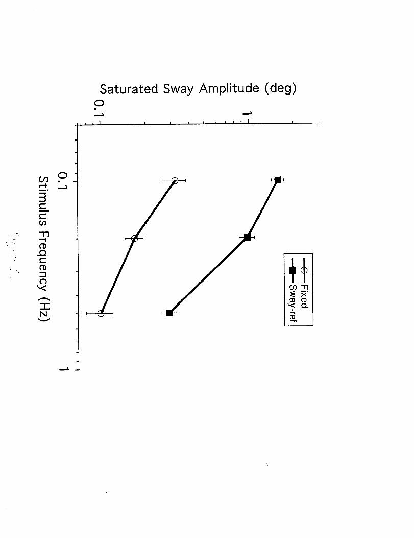
Saturated Sway Amplitude (deg)0

I I I I I I I I I I I I

g

A (i) (ii) (iii)r

// r / rlj

+s /l+s f s

B

c-

r,Drr0

0.8

I

I

|

!

I

|

I

0

y = 0.20 x 0.25°

' I ' I ' I ' I ' I

20 40 60 80 100

Stimulus Amplitude (deg)