Roger Tourangeau, Michele Zimowski, Rashna … · Roger Tourangeau, Michele Zimowski, and ... Peter...

AN INTRODUCTION TO PANEL SURVEYS IN

TRANSPORTATION STUDIES

Roger Tourangeau,Michele Zimowski,

andRashna Ghadialy

Prepared for: NORCFederal Highway Administration 1155 60 Streetth

October, 1997 Chicago, IL 60615(773) 753-7500

ACKNOWLEDGMENTS

We are grateful for the help we received from many quarters. Judy Brint andImelda Perez, of NORC’s editorial staff, formatted the final version of this reportand corrected many a typo and grammatical error along the way; we are gratefulfor their careful work on the report. We thank the members of our advisory panel,who gave us comments and suggestions on our earlier drafts. These include:

Ed Christopher, Chicago Area Transportation Study;Bob Griffiths, Metropolitan Washington COG;Konstadinos Goulias, Pennsylvania State University;Arnim Meyburg, Cornell University;Paul Moore, Research Triangle Institute;Peter Stopher, Louisiana State University;Johanna Zmud, NuStats.

In addition, Eric Pas of Duke University and Ryuichi Kitamura of KyotoUniversity provided detailed technical advice and input to the report. Their helpwas essential to this effort and we gratefully acknowledge their contributions tothe report. Elaine Murakami and Jerry Everett provided oversight from theFederal Highway Administration. They were both gentle task masters; it was apleasure to work with them.

TABLE OF CONTENTS

ACKNOWLEDGMENTS . . . . . . . . . . . . . . . . . . . . . . . . . . . . . . . . . . . . . . . . . . . . . . . . . . . . . . . i

1. EXECUTIVE SUMMARY . . . . . . . . . . . . . . . . . . . . . . . . . . . . . . . . . . . . . . . . . . . . . . . . . . . 1-1

2. INTRODUCTION . . . . . . . . . . . . . . . . . . . . . . . . . . . . . . . . . . . . . . . . . . . . . . . . . . . . . . . 2-1

2.1 CROSS-SECTIONAL AND PANEL DESIGNS . . . . . . . . . . . . . . . . . . . . . . . . 2-1

3. CROSS-SECTIONAL VS. LONGITUDINAL DATA FOR

SURVEYS ON TRAVEL BEHAVIOR . . . . . . . . . . . . . . . . . . . . . . . . . . . . . . . . 3-1

3.1 USES OF PANEL AND CROSS-SECTIONAL DATA . . . . . . . . . . . . . . . . . . . 3-1Developing Travel Demand Models andForecasting Future Demand . . . . . . . . . . . . . . . . . . . . . . . . . . . . . . . . . . 3-1Measuring and Understanding Trends inPopulation Behavior . . . . . . . . . . . . . . . . . . . . . . . . . . . . . . . . . . . . . . . 3-4Conducting Behavioral Analysis . . . . . . . . . . . . . . . . . . . . . . . . . . . . . . . 3-4Impact Assessments . . . . . . . . . . . . . . . . . . . . . . . . . . . . . . . . . . . . . . . . 3-5

3.2 OTHER ADVANTAGES OF PANEL DESIGNS . . . . . . . . . . . . . . . . . . . . . . . 3-73.3 SPECIAL PROBLEMS WITH PANEL DESIGNS . . . . . . . . . . . . . . . . . . . . . . . . 3-8

4. ISSUES IN CONDUCTING A PANEL SURVEY . . . . . . . . . . . . . . . . . . . . . . . . . . 4-1

4.1 OVERVIEW . . . . . . . . . . . . . . . . . . . . . . . . . . . . . . . . . . . . . . . . . . . . . . . . 4-14.2 DESIGN ISSUES . . . . . . . . . . . . . . . . . . . . . . . . . . . . . . . . . . . . . . . . . . . . . 4-3

Definition of the Sample Unit . . . . . . . . . . . . . . . . . . . . . . . . . . . . . . . . . 4-3The Number and Spacing of Rounds . . . . . . . . . . . . . . . . . . . . . . . . . . . 4-4Method of Data Collection . . . . . . . . . . . . . . . . . . . . . . . . . . . . . . . . . . 4-5Sample Size . . . . . . . . . . . . . . . . . . . . . . . . . . . . . . . . . . . . . . . . . . . . . 4-6

4.3 MAINTAINING THE PANEL . . . . . . . . . . . . . . . . . . . . . . . . . . . . . . . . . . . . 4-8Freshening the Sample . . . . . . . . . . . . . . . . . . . . . . . . . . . . . . . . . . . . . 4-8Maintaining High Response Rates Across Waves . . . . . . . . . . . . . . . . . . . 4-9Modifying the Questionnaires Across Rounds . . . . . . . . . . . . . . . . . . . . 4-12

5. WEIGHTING PANEL DATA . . . . . . . . . . . . . . . . . . . . . . . . . . . . . . . . . . . . . . . . . . . 5-1

5.1 WEIGHTS FOR THE INITIAL WAVE . . . . . . . . . . . . . . . . . . . . . . . . . . . . . . . 5-15.2 PANEL WEIGHTS . . . . . . . . . . . . . . . . . . . . . . . . . . . . . . . . . . . . . . . . . . . . 5-2

6. SUMMARY . . . . . . . . . . . . . . . . . . . . . . . . . . . . . . . . . . . . . . . . . . . . . 6-1

TABLE OF CONTENTS (Continued)

APPENDICES

A.1 WEIGHTING DATA FROM THE INITIAL WAVE . . . . . . . . . . . . . . . . . . . . . . A-1A.2 DEVELOPING PANEL WEIGHTS . . . . . . . . . . . . . . . . . . . . . . . . . . . . . . . . . A-4

GLOSSARY OF TERMS . . . . . . . . . . . . . . . . . . . . . . . . . . . . . . . . . . . . . . . . . . . . . . . . . G-1

REFERENCES . . . . . . . . . . . . . . . . . . . . . . . . . . . . . . . . . . . . . . . . . . . . . . . . . . . . . . . . . R-1

SUGGESTED READINGS . . . . . . . . . . . . . . . . . . . . . . . . . . . . . . . . . . . . . . . . . . . . . . . . S-1

AN INTRODUCTION TO PANEL SURVEYS IN TRANSPORTATION STUDIES 1–1

1. EXECUTIVE SUMMARY

This report is a general introduction to the use of panel designs in surveys of travelbehavior. It has four main objectives:

to highlight the differences between cross-sectional and panel approaches tothe study of travel behavior,to discuss the limitations of cross-sectional and panel data,to identify situations where panel data are preferable, andto provide guidelines for designing and maintaining a panel survey.

The report contains a number of recommendations concerning the conduct and useof panel designs in travel surveys. They are summarized below.

GUIDELINES FOR CONSIDERING A PANEL DESIGN

Consider using a panel design whenever the purpose of the travel survey is:

to develop travel demand models and forecast future demand,

to measure and understand trends in population behavior,

to assess the impact of a change in transport policy or services, or

to collect timely information on emerging travel issues.

GUIDELINES FOR DESIGNING AND CONDUCTING A PANEL SURVEY

Use the household as the sampling unit and follow initial respondents as theymove to new households.

Collect data from respondents once a year unless more frequent data arerequired to meet the objectives of the survey.

Add a supplemental sample of households to improve the representativeness ofthe panel if the composition of the population in the study area undergoessubstantial changes during the survey period, or if the survey continues for fiveor more years.

SECTION 1

1–2 AN INTRODUCTION TO PANEL SURVEYS IN TRANSPORTATION STUDIES

To reduce panel attrition, maintain contact with respondents between waves,develop a locating protocol for tracing respondents who move, giverespondents small cash incentives in advance of their participation, and droponly hardcore refusals from the panel.

Add new modules to the survey instruments as new issues arise, but change thecore instruments only when absolutely necessary.

Weight the data to produce unbiased estimates of population behavior.


2.INTRODUCTION

Over the past few decades, several hundred travel surveys have been conductedwithin the United States, mostly by regional transit agencies and metropolitanplanning organizations [1]. The data from these surveys have been used for suchdiverse purposes as measuring the impact of changes in the transportation systemon travel behavior, forecasting future travel patterns and demand, and developingmarketing campaigns to promote transit use. Nearly all the surveys have relied oncross-sectional designs that measure variation in travel behavior among themembers of a population.

The purpose of this report is to discuss a different kind of survey design thatmeasures variation in travel behavior at the level of the individual household orperson by taking repeated measurements on the same sample of units at differentpoints in time. These designs, referred to as panel or longitudinal designs in thesurvey literature, provide direct information on how the travel behavior ofindividual households or persons changes over time in response to other factors.

Although panel designs have enjoyed widespread use in transportation studies inother countries, and in work in other fields, they have rarely been adopted in travelsurveys in the United States. This report shows how they can be used to address avariety of transportation policy and planning issues, ranging from impactassessments of specific policy changes on travel behavior to the more generalissues of predicting and planning for future trends in behavior.

The report begins by describing the differences between panel and cross-sectionalapproaches to the study of travel behavior. It then discusses the advantages andlimitations of these approaches to data collection, identifies situations where paneldata are desirable, and illustrates their benefits through examples drawn from thetransportation literature. The final section of the report provides guidelines for theconduct of panel surveys, focusing on the special issues and difficulties that arisewhen the same sample of households or individuals is measured repeatedly overtime.

2.1. CROSS-SECTIONAL AND PANEL DESIGNS

All surveys can be classified into one of two broad categories on the basis ofwhether they obtain repeated measurements on the same sample of units over time. Panel surveys do and cross-sectional surveys do not.

Within these two approaches to data collection, surveys may be furtherdistinguished according to whether they monitor changes in the population overtime. Cross-sectional and panel surveys that incorporate this feature periodically

SECTION 2


draw new samples from the population and collect measurements on them usingthe same methods as in previous time periods.

The differences among these four approaches to the collection of survey data aresummarized in Table 1. The table distinguishes between two types of cross-sectional designs—one-time cross-sectional designs, and repeated cross-sectionaldesigns—and two types of panel designs—longitudinal panel designs, androtating or revolving panel designs. It shows how the designs differ along fourdimensions:

the number of distinct samples in the survey,

the number of time points or measurement periods,

the number of measurements per sample member, and

the types of differences measured.

INTRODUCTION

Table 1

Differences Among the Features of Four Types of Survey Designs

Approach Design Samples Time Points Member Variation) Variation) Across Time

Number of Measurements Members Across Time theDistinct Number of Per Sample (Cross-sectional (Longitudinal Population

Number of Among Sample Members Variation in

Type of Variation Measured

Variation Within SampleVariation

Cross-sectional

One-timecross-sectional one one one Yes No No

designs

Repeated cross-sectional two or more one Yes No Yes

designs

two or more(same as the

number of timepoints)

Panel(Longitudinal)

Longitudinal (same as thepanel designs numberone two or more Yes Yes No

two or more

of time points)

Rotating panel (generally lessdesigns than the numbertwo or more two or more Yes Yes Yes

two or more

of time points)


SECTION 2


One-time cross-sectional surveys. In the United States, most travel surveysrely on one-time cross-sectional designs to collect information on travelconsumption and behavior. In these designs, a single sample of households orindividuals, usually a cross section of the regional or national population, is askedto complete a survey at a single point in time. In other words, a single set ofmeasurements is collected from each sample member. In practice, the time atwhich the measurements are actually taken varies somewhat across samplemembers. Nevertheless, the measurements are close enough in time to be regardedas contemporaneous, as occurring at the same point or period in time.

One-time cross-sectional designs capture the travel behavior of the population as itexists at the time of the survey. They provide a “snapshot” of travel behavior in aregion by obtaining snapshots of the behavior of the individual sample members. Surveys of this type measure cross-sectional variation in travel behavior, that is,variation among the members of a population. They show how behavior differsfrom member to member, but they provide no direct information on how it changesover time.

A distinguishing feature of one-time cross-sectional surveys is that they make noattempt to replicate conditions of previous surveys. They may measure a similarset of variables, but the actual questions posed to the respondents may differ inwording or in meaning, and the sampling and field procedures may not be the sameas in previous surveys. For this reason, one-time cross-sectional surveysconducted at different points in time are not well suited for assessing trends inpopulation behavior since their results cannot be readily compared with oneanother.

Repeated cross-sectional surveys. Repeated cross-sectional designs, on theother hand, measure the travel behavior or attitudes of the population over timeby repeating the same survey on two or more occasions. During each time period,a separate but comparable sample of units is drawn from the population and askedto complete the survey. Each sample member completes the survey once, unlessthey are selected by chance into more than one sample.

Because the field procedures, survey instruments, and samples are comparablefrom period to period, designs of this type allow for comparisons among andbetween measurement periods. They are ideally suited for assessing period trendsin behavior at the population or other aggregate levels, and are often used tomonitor changes in the population as a whole or in various subgroups within thepopulation, such as those defined by demographic background characteristics. However, they provide no direct information on change at the level of theindividual sample member since each measurement period relies on a distinctsample of households or individuals. Like one-time cross-sectional surveys, they

INTRODUCTION

A survey in which respondents are asked to report their activities or travel behavior for a period of two or1

more consecutive days could also be considered a “longitudinal” survey, but this is not standard usage of the term. These “multi-day” surveys measure daily variation in travel behavior during a single time period. Longitudinalsurveys, as defined here, measure variation in the behavior of individual sample members over two or more periodsin time.


measure cross-sectional variation in travel behavior, but at two or more periods intime instead of at one.

Repeated cross-sectional designs are often referred to as longitudinal designs in thesurvey literature because they measure variation in the population over time. Following the convention adopted in the Travel Survey Manual, we reserve theterm longitudinal to refer to designs that collect measurements on the same sampleof units at different times. Such designs are discussed below.1

Longitudinal panel surveys. Longitudinal panel designs differ from cross-sectional surveys in that they collect information on the same set of variables fromthe same sample members at two or more points in time. For a household travelsurvey, this means that the same sample of households is asked to answerquestions about their travel behavior and other variables on two or moreoccasions. Each distinct occasion when data are collected from the samplemembers is referred to as a wave or round of data collection. In a two-wave panelsurvey, sample members are asked to provide data twice, once during each wave. In a three-wave panel survey, panel members are asked to provide data threetimes, and so on. Within each wave the measurements are close enough in time tobe considered contemporaneous. Typically, each wave collects some of the sameitems of information and some new items as well.

Although there is no upper limit on the number of waves a panel survey maycontain, in practice most panel surveys consist of between 2 and 10 waves. Thisfeature is often used to distinguish them from time series, which collect a series ofmeasurements over a relatively large number of time points. Time series differfrom panel surveys in two other important respects: 1) they collect data on asingle entity, such as a person or a nation, while panel surveys obtainmeasurements on a collection of units, usually individuals or households, and 2)the time point rather than the individual sample member is the unit of analysis.

Longitudinal panel surveys are similar to cross-sectional surveys in that theymeasure cross-sectional variation in travel behavior by collecting information on asample of units. What sets them apart from cross-sectional surveys is that theyalso measure longitudinal variation in travel behavior—that is, variation over timeat the level of the individual sample member—by repeating the survey on the samesample of units at two or more points in time. In other words, they provideinformation on how the travel behavior of individual sample members changes overtime in response to changes in the travel environment, household backgroundcharacteristics, or other factors.

SECTION 2


Longitudinal panel surveys are similar to repeated cross-sectional designs in thatthey permit comparisons across time by asking the same questions undercomparable conditions. But, unlike repeated cross-sectional designs, they ask thequestions of the same sample members and thus provide for direct measurement ofindividual change.

During the first wave of data collection, longitudinal panel surveys provide thesame information as one-time cross-sectional designs. They assess currentpopulation levels and measure cross-sectional variation in travel behavior. Duringthe second and subsequent waves, longitudinal panel surveys also measure cross-sectional variation, but they may not measure current population levels since thecomposition of the current population may no longer be the same as it was in thefirst wave when the sample was drawn. However, if the time span of the survey isrelatively short and the panel sample is periodically refreshed, chances are high thatdata obtained in each wave will reflect current population levels.

Revolving or rotating panel designs. Rotating or revolving panel surveysare a combination of repeated cross-sectional and panel designs. They collectpanel data on the same sample of units for some specified number of measurementperiods. Portions of the sample are then gradually dropped from the panel andreplaced with new but comparable samples drawn from the current population. The process of retiring portions of the existing sample and adding new members tothe sample continues until the original panel is completely replaced. The newsample members are retained in the survey for some specified number ofmeasurement periods and then gradually replaced with a comparable but morecurrent sample and so on. The survey may continue indefinitely or be limited to acertain number of replacement samples. Each sample of units selected at the sametime and adhering to the same schedule of data collection is called a rotationgroup.

The strength of rotating panel designs lies in their ability to allow for short-termanalysis of individual or household change and long-term analysis of populationand subgroup change. As in panel surveys consisting of a single sample of thepopulation, rotating panel designs provide direct information on change at the levelof the individual household or person over the period in which the sample memberis retained in the survey. As in repeated cross-sectional designs, they provideinformation on how travel behavior changes over time at the population or otheraggregate levels by periodically drawing comparable samples from the currentpopulation and obtaining similar measurements on them.

Other variations. Although most surveys fall into one of these four categories,there are many variations within each category not discussed here. For example, itis possible to have a rotating panel design in which portions of a sample are retiredfrom the survey for some specified number of time periods and then returned tothe survey for additional measurement periods.

AN INTRODUCTION TO PANEL SURVEYS IN TRANSPORTATION STUDIES 3-1

3. CROSS-SECTIONAL VS. LONGITUDINAL DATA

FOR SURVEYS ON TRAVEL BEHAVIOR

3.1 USES OF PANEL AND CROSS-SECTIONAL DATA

The most obvious and important benefit of panel surveys is that they directly measurebehavioral change at the level of the individual sample member and thus supplyinformation that cannot be obtained in a cross-sectional survey. By virtue of thisfeature, they provide a rich source of information that can be used to arrive at a betterunderstanding of the factors that influence and control personal travel behavior. Thisinformation is important whenever the purpose of the travel survey is:

to develop travel demand models and forecast future demand (e.g., to developmodels of transit mode share and to predict transit mode share following theintroduction of a new rail line),

to measure and understand trends in population behavior (e.g., to measurechange in the average household trip rate and understand why the rate haschanged or remained constant),

to conduct behavioral analyses (e.g., to determine fare or travel time elasticity),or

to assess the impact of a change in transport policy or a change in thetransportation system (e.g., to measure changes in travel behavior followingthe opening of a new rail line) [2].

The sections below discuss why panel designs are preferable in these situations.

DEVELOPING TRAVEL DEMAND MODELS AND FORECASTING FUTUREDEMAND

Although cross-sectional data are well suited for assessing current levels of traveland for measuring period trends in population behavior, they provide only indirectinformation on the determinants of personal travel behavior. Nonetheless, thisinformation, in the form of differences across households or individuals, forms thebasis for most predictive models of personal travel behavior. These models assumethat household or individual changes in personal travel behavior can be predictedon the basis of cross-sectional differences in behavior across households or persons[3]. Since these models are based on data from a single point in time, they areoften referred to as “static” models in the literature. (Models based on panel dataare typically referred to as “dynamic” models, on the other hand.)

For illustrative purposes, suppose one wanted to predict how the automobile tripfrequency of a one-car household would change if it acquired an additionalautomobile. In models relying on cross-sectional data, this change in trip

SECTION 3

3-2 AN INTRODUCTION TO PANEL SURVEYS IN TRANSPORTATION STUDIES

frequency would be predicted on the basis of the difference in trip frequenciesbetween one- and two-car households.

This type of inference assumes that several restrictive conditions are met:

the changes are instantaneous,

the changes are the same in either direction, and

the relationship among variables is stable or invariant over time [3].

In terms of the example above this means:

the acquisition of the additional automobile and the change in trip frequencyoccur simultaneously,

a reversal—a change back to one automobile—returns the household to itsprevious travel rate, that is, the same frequency of trips as before, and

the relationship among the number of automobiles and trip frequency remainsthe same over time.

Recent studies challenge the validity of these assumptions and the suitability ofcross-sectional data for predicting changes in travel behavior. A study based ondata from the Dutch National Mobility Panel (DNMP), for example, offersempirical evidence that changes in trip frequency and employment status do notoccur simultaneously, as assumed in cross-sectional models [4]. In the study,sample members were divided into four groups according to their employmentstatus in the first and second waves of the survey: employed - employed;employed - not employed; not employed - employed; and not employed - notemployed. Analysis of changes in trip frequencies within these groups revealedstrong inertia effects; trip frequencies did not change very much regardless ofchanges in employment. The average trip rate of male adults in the “not employed- employed” group, for example, was smaller than the sample average by 0.9 tripsin the first wave, and remained smaller than the sample average by 0.7 trips in thesecond wave. The average rate of male adults in the “employed - employed”group, on the other hand, was greater than the sample average by 0.7 trips in thefirst wave, and 0.9 trips in the second wave. In other words, trip rate changesfrom the first to second wave were about equal for both groups. These resultssuggest that changes in employment status do not immediately produce a drop orgain in trip frequency as assumed in models of cross-sectional data.

A simple example that compares regression coefficients from static and dynamicmodels of travel behavior also illustrates how the predictions of travel demand modelsmay be affected when they are based on cross-sectional versus panel data [5]. For theexample, a static model was fit to the cross-sectional data from a panel survey

CROSS SECTIONAL VS. LONGITUDINAL DATA


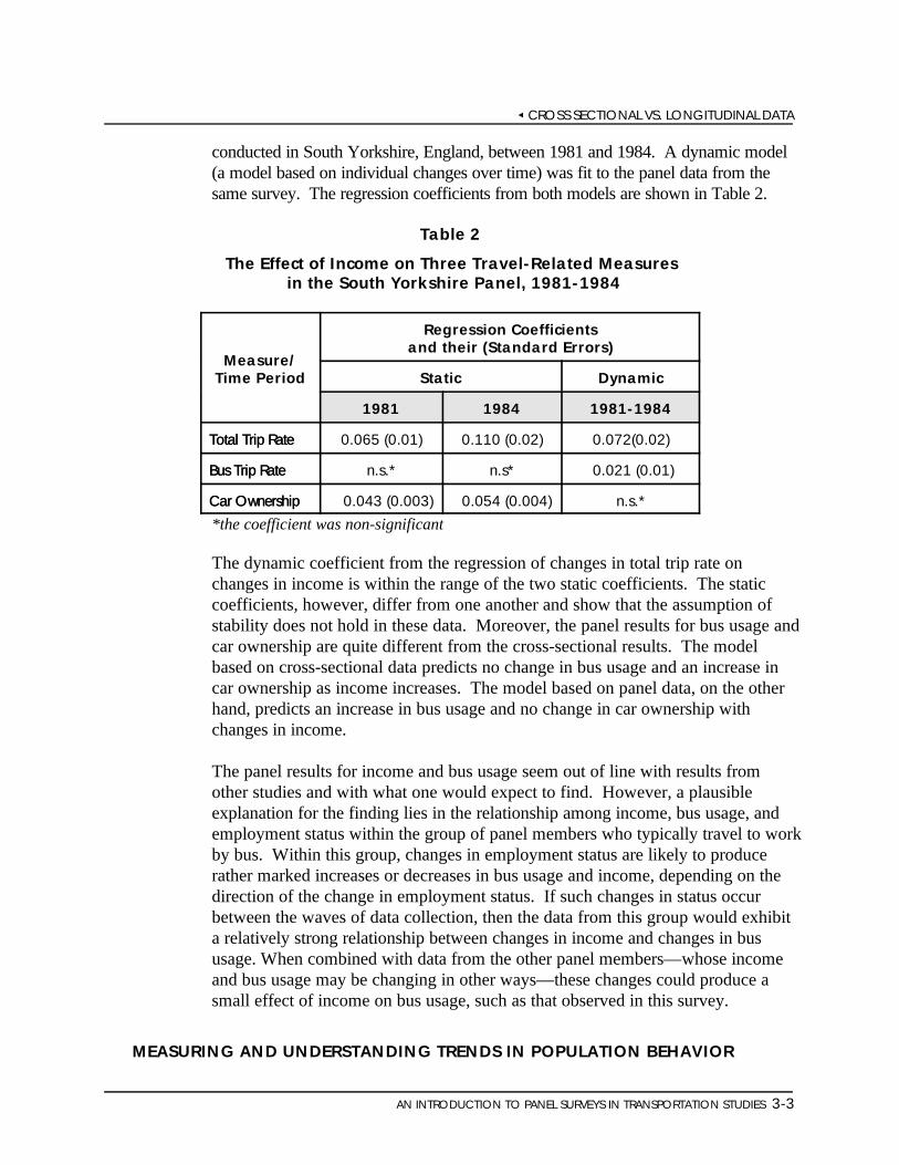
conducted in South Yorkshire, England, between 1981 and 1984. A dynamic model(a model based on individual changes over time) was fit to the panel data from thesame survey. The regression coefficients from both models are shown in Table 2.

Table 2

The Effect of Income on Three Travel-Related Measures in the South Yorkshire Panel, 1981-1984

Measure/Time Period Static Dynamic

Regression Coefficientsand their (Standard Errors)

1981 1984 1981-1984

Total Trip RateTotal Trip Rate 0.065 (0.01) 0.110 (0.02) 0.072(0.02)

Bus Trip RateBus Trip Rate n.s.* n.s* 0.021 (0.01)

Car OwnershipCar Ownership 0.043 (0.003) 0.054 (0.004) n.s.*

*the coefficient was non-significant

The dynamic coefficient from the regression of changes in total trip rate onchanges in income is within the range of the two static coefficients. The staticcoefficients, however, differ from one another and show that the assumption ofstability does not hold in these data. Moreover, the panel results for bus usage andcar ownership are quite different from the cross-sectional results. The modelbased on cross-sectional data predicts no change in bus usage and an increase incar ownership as income increases. The model based on panel data, on the otherhand, predicts an increase in bus usage and no change in car ownership withchanges in income.

The panel results for income and bus usage seem out of line with results fromother studies and with what one would expect to find. However, a plausibleexplanation for the finding lies in the relationship among income, bus usage, andemployment status within the group of panel members who typically travel to workby bus. Within this group, changes in employment status are likely to producerather marked increases or decreases in bus usage and income, depending on thedirection of the change in employment status. If such changes in status occurbetween the waves of data collection, then the data from this group would exhibita relatively strong relationship between changes in income and changes in bususage. When combined with data from the other panel members—whose incomeand bus usage may be changing in other ways—these changes could produce asmall effect of income on bus usage, such as that observed in this survey.

MEASURING AND UNDERSTANDING TRENDS IN POPULATION BEHAVIOR

SECTION 3


Repeated cross-sectional designs yield measurements of period trends inpopulation behavior, but they do not further our understanding of why the changesoccur. Panel designs yield similar information but also allow for analysis of theunderlying causes by providing information on the changes occurring to individualmembers of the population. Aggregate measures of change tend to mask thesechanges and often lead to erroneous conclusions of stability, even when thebehavior of the individuals is volatile.

Cross-sectional data from the South Yorkshire Panel Survey of car ownership, forexample, show modest increases in net car ownership, ranging from about 2 to 6percent during each time interval (see Table 3) [5]. The panel data, on the otherhand, indicate that ownership levels were quite volatile during this time period. Between 21 and 26 percent of the population changed their level of ownershipduring each time interval. Moveover, between 13 and 15 percent acquiredadditional automobiles, while about 7 to 12 percent reduced their level ofownership. Since these changes differ in direction, they tend to cancel one anotherout when measurements are based on cross-sectional data. For this and otherreasons, aggregate measures of change tend to provide an inaccurate picture ofchanges occurring to members of the population.

Table 3

Changes in Car Ownership of the South Yorkshire Panel

Changes inLevel of CarOwnership

Time Interval

1981-1984 1984-1986 1986-1988 1988-1991

OwnershipReductions 10.5% 8.6% 7.2% 11.6%

No Change 76.4% 78.5% 79.1% 73.7%

OwnershipIncreases 12.8% 12.9% 13.6% 14.6%

Net Increasein Car 2.3% 4.3% 6.4% 3.0%

Ownership

CONDUCTING BEHAVIORAL ANALYSIS

Cross-sectional surveys provide sufficient data for examining travel behavior at asingle point in time and for analyzing and modeling differences in travel behavioracross individuals, but they reveal very little about the dynamics of personal travelbehavior. Cross-sectional data, for example, show that public transportation usageis negatively correlated with automobile ownership, but they can not predict howmuch an individual’s usage might change following a change in car ownership.



Data from six waves of the DNMP illustrate this point [5]. Static correlationsbetween public transport usage and car ownership are in the order of -0.20 suggesting that an increase in car ownership will lead to a moderate decreasein use of public transit. The dynamic correlations are in the order of -0.05 showingthat changes in car ownership have little effect on an individual’s use of publictransportation.

IMPACT ASSESSMENTS

Before-and-after designs are commonly used in transportation surveys to study theimpact of transport services and policy on travel behavior, attitudes, and safety. Instudies of this type, the phenomenon of interest is measured before and after achange in services or policy to assess the impact of the change. Examples of suchstudies include:

assessments of the impact of new legislation on travel behavior (e.g., reductionin trip frequencies following the passage of telecommuting laws),

evaluations of the effects of improvements to the transportation system (e.g.,reductions in fatality and injury rates following the construction of roadsidebarriers), and

examinations of the impact of new technologies on traffic flow patterns andattitudes (e.g., changes in travel behavior and attitudes following theintroduction of changeable message signs or Advanced Traveler InformationSystems).

In one such survey conducted in Almere, Netherlands sample members were askedto report their mode of transportation to the workplace, along with otherinformation—such as car availability—before and after the opening of a newrailway line [6, 7]. In a similar study conducted in San Diego, sample memberswere asked to report their travel behavior and attitudes before and two times aftera roadway for high-occupancy vehicles was opened on Interstate 15. The secondand third waves of data were used to evaluate short- and long-term effects of theroadway on personal travel behavior [8].

In assessments of this type, the advantages of a panel design are clear. Incomparison to a repeated cross-sectional design, a panel design:

requires a smaller sample size to measure change over time,

costs substantially less if the number of time points is relatively small, and

permits examination of individual differences in the direction and magnitude ofchange.

SECTION 3


To illustrate the type of information that would be lost if a repeated cross-sectionalsurvey was adopted instead, data from the Almere study are shown in Tables 4 and5. Table 4 displays the type of aggregate-level information that would be obtainedin a repeated cross-sectional design and in a panel design. It shows the numberand percent of sample members who traveled to work by car, train, or bus beforeand after the opening of the new railway line. According to these data, the levelof travel by car remained the same across time, while bus use substantially declinedafter the opening of the railway.

Table 4

Mode of Transportation to the Workplace Before andAfter the Opening of the Rail Line

Mode Choice Number Percent Number Percent

Before After

Car 320 67.4% 321 67.6%

Train — — 119 25.1%

Bus 155 32.6% 35 7.4%

The data in Table 5, available only in a panel survey, provide a more completepicture of the effects of the railway line on travel patterns. Of the 320 individualswho originally traveled to work by car, 27 or (about 8 percent) switched to trainwhile 5 (or roughly 2 percent) switched to bus. But, more surprisingly, 33 (orroughly 21 percent) individuals who originally traveled to work by bus chose todrive to work after the opening of the line. Without the benefit of a panel design,these turnovers in mode use would be missed.

Table 5

Change in Mode of Transportation

ModeChoiceBefore Number Percent Number Percent Number Percent

Mode Choice After

Car Train Bus

Car 288 90.8% 27 8.4% 5 1.6%

Bus 33 21.3% 92 59.4% 30 19.3%

nc np × 1

1 R,

R

1 R1 R

nc

np

0.201/ 0.20



3.2 OTHER ADVANTAGES OF PANEL DESIGNS

In addition to providing for direct measurement of change, panel surveys offer anumber of other practical and analytical benefits. These benefits include:

increased statistical efficiency,

timely information about emerging travel issues, and

reduced cost relative to cross-sectional surveys.

Statistical efficiency. When the same sample of units is used in all time periods,estimates of change over time become more precise. This is because in panelsurveys comparisons across time periods are free from some of the effects ofrandom sampling error. As a result, panel surveys require a smaller sample sizethan repeated cross-sectional surveys to measure aggregate change with the samelevel of precision. For simple statistics like averages or proportions, the reductionin sample size depends on the correlation over time in the variable of interest (forexample, the number of cars available to the household).

If is the correlation between the measurements of a variable over time, then thevariance of the estimate of change (the difference between measurements at time 1and time 2) is reduced by a factor of , while the standard error of the estimateis reduced by a factor of [9]. This means that separate cross-sectionalsamples of size , where

are required to measure change with the same level of precision as that providedby a panel sample of size .

In cases where the correlation between measurements is high, the gains inefficiency can be quite large. Kish, for example, reports the results of a survey oncar ownership in which the measurements correlate 0.8 over time [10]. In this case,the variance of the difference between the measurements is reduced by a factor of0.20, the standard error by a factor of . In terms of the formula above, thismeans that the cross-sectional samples must be or roughly 2.24 timeslarger than the panel sample to yield estimates of equal precision as measured bytheir standard errors.

nc np × 1

1 0.20np × 2.24

SECTION 3


Timely source of travel information. Once a panel survey is in place, it canserve as an ongoing source of up-to-date information about travel behavior. Newdata can be examined as they become available, and questions can be added to thesurvey instrument as needed to address current concerns and policy issues. It isoften far easier and faster to add supplemental questions in an existing panel thanto mount a whole new survey to acquire the same information. The extent towhich a panel survey will serve this purpose should be decided in advance of thesurvey since it may affect the content and length of the core questionnaire.

Cost savings. Because panel surveys measure the same sample across timeperiods, sampling and respondent recruitment costs are considerably lower thanthose for repeated cross-sectional designs, where a new sample must be drawn andrecruited during each time period. In later waves, these savings may be offsetsomewhat by the extra effort required to “feed and maintain” a panel sample. However, if the design includes only a few waves, a panel survey should costconsiderably less than a repeated cross-sectional survey with the same number ofmeasurement periods. The savings include some or all of the instrumentdevelopment and pretesting costs, the costs of screening and recruiting the initialsample, and much of the costs of developing systems for monitoring the field effortand processing the data. Depending on the exact design, the costs ofreinterviewing a panel may be 20 to 80 percent less than the costs of obtaining thesame information from a new sample. Lawton and Pas estimate that the cost persample household in subsequent waves of a travel panel survey is about 50 percentof the cost in the first wave [11].

3.3 SPECIAL PROBLEMS WITH PANEL DESIGNS

If panel surveys have advantages over cross-sectional designs, they also havecertain drawbacks [12]. These include:

panel attrition, or nonresponse in later waves of data collection;

time-in-sample effects, or the effect of prior reporting on reporting insubsequent waves of data collection [13];

seam effects, or an apparent increase in the number of changes across roundsof a survey as compared to the number observed within each round [14].



In a panel survey, the effects of nonresponse in the initial wave of data collectionare compounded over time as initial respondents drop out in subsequent waves. The cumulating impact of nonresponse across waves of data collection is calledpanel attrition. As panel attrition increases, the sample becomes less and lessrepresentative of the cohort it was selected to represent.

To illustrate the cumulative effects of nonresponse, Table 6 shows the number ofrespondents who participated in each of the first four waves of the Puget SoundTransportation Panel (PSTP). About 33 percent of eligible members in the originalsample took part in the first wave of data collection. Only about 55 percent ofthose original respondents completed the fourth wave of data collection in 1993. In other words, only 18 percent of the original sample of eligible membersremained in the survey after the fourth round of data collection.

Table 6

Number of Respondents and Percent of Original Sample in theFirst Four Waves of the Puget Sound Transportation Panel

Year 1989 1990 1992 1993

Wave 1 2 3 4

Number ofRespondents 1,713 1,385 1,080 935

Percent oforiginal panel — 81% 63% 55%

Similar information for the Dutch National Mobility Panel is shown is Table 7. After the first year of data collection, which consisted of two waves, the DNMPretained about 58 percent of the original respondents. By the end of the survey,only about one third of the original respondents remained in the panel.

Table 7

Number of Respondents and Percent of Original Sample inSelected Waves of the Dutch National Mobility Panel

Year 1984 1985 1986 1987 1988 1989

Wave 1 3 5 7 9 10

Number ofRespondents 1,764 1,031 853 668 629 576

Percent oforiginal panel — 58% 46% 38% 36% 33%

SECTION 3


Reporting errors can also increase among those who remain in the panel over time. There are several terms for such time-in-sample effects, including conditioning[15], rotation bias [16], and panel fatigue [14]. All three terms refer to the samegeneral phenomenon: respondents tend to report fewer trips, spells ofunemployment, household repairs, and consumer purchases in the later rounds of apanel survey than in the earlier ones.This pattern of reporting is evident in data from the DNMP [17 ]. According to aregression model fit to those data, participants in the first wave reported about 2.27 fewer trips per week than expected, while participants in the seventh wavereported about 8.35 fewer trips per week than expected. Table 8 shows how themagnitude of underreporting increased over time as participants completed morerounds.

Table 8

Estimated Number of Unreported Trips Per Week by Wave

Wave 1 2 3 4 5 6 7

Numberof Trips 2.27 4.44 5.70 6.60 7.20 7.87 8.35

In some cases, a drop in reporting can be observed within a single round; forexample, respondents tend to report more consumer purchases in the first few daysof keeping a diary than in the last few days, even in the initial wave of a panelsurvey. A number of studies have examined whether respondents in travel surveysdisplay this pattern of reporting as they complete multi-day diaries. The results ofthe studies are mixed. Analysis of 1984 data from the seven-day travel diary of theDutch National Mobility Panel, for example, revealed that trip reporting decreasedover time largely because more respondents reported no trips at all over time [18]. Analysis of data from a three-day travel survey conducted in Seattle in 1989, onthe other hand, found no evidence of decreased levels of diary reporting in thesecond and third days [19].

Another kind of reporting error may affect panel surveys that collect informationabout the entire period between rounds of data collection. In such surveys,respondents might be asked to report the amount they earned in each month sincethe prior interview. In these types of designs, there is a tendency for respondentsto report changes as occurring at the beginning or end of the time interval betweenrounds rather than at other times covered by the interview. Changes in salary, forexample, seem to cluster in the first month covered by the interview. This patternof reporting is called the seam effect; it reflects the effect of faulty memory forwhen changes took place [14].



In summary, then, panel designs can compound the problems of nonresponse biasand reporting errors that are also found in cross-sectional surveys.


4.ISSUES IN CONDUCTING

A PANEL SURVEY

4.1 OVERVIEW

There are numerous choices that must be made during the design andimplementation of a panel survey. These include such basic issues as:

the definition of the sampling unit (households, addresses, or persons),

the choice of a sample size,

the addition of cases to the sample to maintain the size of the sample, itsrepresentativeness, or both,the number and spacing of rounds of data collection,

the method (or combination of methods) to be used in collecting the data,

the tracing of households and individuals who move between rounds,

the use of incentives, and

the use of other techniques to reduce attrition.

Current practice. To help frame our discussion of these issues, Table 9 presentsthe relevant features of two general-purpose travel panels and two other prominentpanel surveys on labor force behavior. These successful panel surveys illustratesome of the common solutions to the problems raised in planning and carrying outlongitudinal studies.

SECTION 4

Table 9

Comparison of Methods Used in Four Panel Surveys

Survey Name Puget Sound Transportation Dutch National Current Population Survey National Longitudinal SurveyPanel (PSTP) Mobility Panel (CPS) of Youth (NLSY)

(DNMP)

Frequency of Data Annually or bi-annually Twice a year Every month on a Annually 1979-1994;

Collection rotational basis of biannually thereafter

4-8-4 months.

Unit Household Household Housing units Individuals and, in somecases, their children

Length of Interval Approx. one or two years March & A month B/w 1979 and 1994, 1 year;September b/w from 1995 on, 2 yearsMarch 1984 &March 1989

Use of Incentives $2 bill, attached to each set of None None Through 1994 $10.00;diaries, for each person who thereafter $20.00completes diaries

Follow-up postcards, etc. Holiday greeting postcard, None None Nonesummary report, letter beforerenewal

Data Collection Method Phone survey & 2-day travel diary A 7-day travel Face-to-face and Face-to-face interviewdiary telephone interview, supplemental data collected

supplementary done by via self-administeredmail survey questionnaire

**Paper-and-pencil personal interview**Computer-assisted personal interview.***Self-administered questionnaire.


ISSUES IN CONDUCTING A PANEL SURVEY

Households are generally defined as groups of people who live together in a single dwelling or housing unit. In1

most definitions, group quarters, such as dormitories and nursing homes, do not qualify as housing units. According to the U.S.Bureau of the Census, a housing unit is a house, apartment, mobile home, group of rooms, or single room with separate kitchenfacilities and with direct access from the outside of the building or through a common hall. To qualify as a housing unit, theoccupants must live and eat separately from other persons in the building. A family, one person living alone, and other groupsof related or unrelated persons who share such living arrangements qualify as households.[20].


4.2 DESIGN ISSUES

DEFINITION OF THE SAMPLE UNIT

With any study design, it is necessary to specify a sampling unit. Most personaltravel surveys use households as their sampling units. The PSTP and the DNMP1

follow this convention [21,22]. Other possible units for travel panels includepersons or housing units.

The issues surrounding the definition of the sample unit can get a little complicatedwhen the study involves a panel design. The complication arises because the unitsmay change over time and one must decide which units to keep in the panel.

When the sampling unit is a person, as in the National Longitudinal Survey ofYouth (NLSY), it is usually clear whether or not to retain the individual in thepanel. Generally, persons who leave the population (for example, by moving outof the study area or by becoming institutionalized) are dropped from the sample,but all others are retained. With both households and housing units, however,things are not so straightforward. Households can divide because of divorce or forother reasons. One member may leave the household and join a different one. New members may be born into a sample household or may join it by marriage oradoption. The sample design must include rules for dealing with each of thesesituations. A common strategy is to collect data from all persons in any householdthat includes at least one respondent from the first round of the survey (providedthat these persons meet the other eligibility criteria for the study, such as living inthe study area). For example, if a household in one wave consisted of a couplethat subsequently splits up, then in later waves both of the resulting householdswould be included in the sample. Similarly, if a new member joins a samplehousehold, then data are collected from that new member. (However, if that newmember subsequently leaves, he or she would not be followed unless his or hernew unit includes a respondent from the first round of the survey.) This strategyentails following respondents who move out of their original household into a newone and collecting data on the other members of the new household. The processof following respondents and collecting data on their households can get a little

SECTION 4

When a sample is drawn from areas with high rental costs or large numbers of students, such as San Francisco or2

Washington, D.C., the number of splits and new combinations is likely to be high since these areas tend to include a highpercentage of single persons living together in households.


Recommendation

complicated when the original panel includes households shared by single personssince splits and new combinations are especially common in this group.2

It is also possible for housing units to subdivide over time into two or more units.(For example, an apartment may be remodeled into two units.) Again, each newunit formed from the units in the original sample should be included in later wavesof the survey. This strategy is followed in the Current Population Survey (CPS),which uses a sample consisting of housing units [23].

CHOOSING A SAMPLING UNIT

Use the household as the sampling unit for panel surveys.Follow initial respondents to new households and add anyadditional household members to the panel.

THE NUMBER AND SPACING OF ROUNDS

Another set of design issues concerns the number and spacing of the rounds orwaves of data collection. The best spacing will depend on such factors as the rateof change in the phenomena of interest and the need for up-to-date information. For example, the more rapidly travel demand is changing, then the more frequentlydata should be collected. Another consideration is the need for timely figures foradministrative or other reporting purposes. The CPS is conducted every month inorder to meet the need for monthly figures on the unemployment rate.

Another consideration affecting the spacing between rounds is the memory burdenimposed by the data collection. Some panel surveys collect a continuous recordfor the entire period between rounds. In each new round of the NLSY, forinstance, respondents are asked to report their employment history for the entireperiod between the current and preceding round of data collection [24]. In suchcases, it is important to keep the spacing between rounds relatively short to reducethe impact of forgetting on the accuracy of the data. The effect of the spacing ofrounds on memory burden does not appear to be a consideration in either thePSTP or the DNMP; in both of these travel panels, the main data collectioninstrument is a multi-day travel diary that covers only a short period precedingeach round.

The DNMP used a six-month interval between waves of data collection. ThePSTP uses a one-year interval (although the PSTP collected some additionalattitudinal data between waves of travel data collection) [21,22]; similarly, theNLSY has used a one-year spacing between rounds for most of its life [24].


The rate of omission from telephone surveys is higher for the unemployed (12 percent of whom live in households3

without telephones) young adults (16 percent of those between the ages of 15 and 24 live in households without telephones),and poor households (more than 20 percent of households with annual incomes of less than $5,000 lack telephones) than fortheir employed, older and wealthier counterparts.


Recommendation

Taken together, the spacing of the waves and the total life of the panel determinethe total level of burden on the respondents. It is unreasonable to expect samplemembers to provide accurate information during many waves of data collectionover a very long period of time. Instead, panel members are likely to drop out andthe quality of the information they provide is likely to decline as the number ofrounds increases. A rotation design can help limit reporting burden on eachmember of the sample. The CPS uses a scheme in which sample membersparticipate for four months, are given eight months off, and then participate forfour additional months [23]. The other illustrative surveys in Table 9 do not userotation designs. The NLSY is now entering its 18th round of data collection andthe PSTP is beginning its 10th round. The DNMP came to an end in March of1989, after 12 rounds of data collection.

COLLECT DATA ONCE A YEAR

Conduct waves of data collection once a year unless morefrequent data collecting is required to obtain the desiredinformation.

METHOD OF DATA COLLECTION

The method used to collect data is another key design decision. Different methodsof data collection differ in terms of cost, coverage of the population, likelyresponse rates, and data quality. Data quality is usually measured in terms of therates of missing or inconsistent information. In general, in-person data collectionis the most expensive, but produces the most complete coverage and highestresponse rates; in addition, it affords greater opportunities for aids to therespondent. Telephone data collection tends to be next most expensive, but omitsthe portion of the population without telephones. Telephone data collection also3

yields lower response rates than in-person data collection. Data quality may suffersomewhat as compared to data collected in a face-to-face interview. Finally, datacollection by mail is the cheapest of the three modes; it offers, in principle,coverage similar to that of in-person data collection, but a lower response rate andpoorer data quality. (When the questions are sensitive, however, a mailquestionnaire may yield more accurate answers because respondents need notworry about an interviewer’s reaction.) These points are summarized in Table 10.

SECTION 4


Recommendation

Table 10

Mode of Data Collection and Their Features

Mode of Data Collection

In-Person Telephone Mail

Description Interviewer travels to Interviewer contacts Questionnaire mailed torespondent’s home or respondent and respondent and isoffice and administers administers questions over returned by mail or dataquestions in face-to-face the telephone retrieved by telephone interview

Coverage Most complete Omits nontelephone Similar to in-person,households depending on how the

addresses are obtained

Response Rate Highest of three modes Intermediate Lowest of three modes

Data Quality Highest of three modes Intermediate Lowest of three modes

Cost Most expensive Intermediate Least expensive

Most personal transportation surveys use a combination of telephone and mail datacollection [1]. Telephone interviews are used to identify eligible householdsinitially and to enlist their cooperation in the main data collection. Then, samplehouseholds are mailed a diary or some other data collection instrument. The datacollection form may be mailed back by the respondents or the informationrecorded on it may be retrieved by telephone. Both the PSTP and the DNMPrelied on some combination of mail and telephone to collect their travel data.

UTILIZE MORE EXPENSIVE MODES IN THE INITIAL WAVEIn the first wave of the survey, contact respondents by telephoneor in-person to maximize the initial response rate. Thereafter,adopt less expensive modes of data collection if necessary.

SAMPLE SIZE

Another key design decision concerns the choice of a sample size for the survey. The process of choosing a sample size usually consists of three steps:

identifying the desired level of precision for the survey estimates,

computing the size of the sample required to obtain estimates at that level, and

adjusting the size to take into account nonresponse, attrition, and eligibilityrates.



Setting the precision level. The process of choosing a sample size begins withan assessment of the amount of error that can be tolerated in the survey estimates. In the case of a panel survey, the assessment usually focuses on the estimates ofchange since they are of primary concern. The objective is to determine howprecise the estimates must be to satisfy the goals of the survey. This determinationrequires information on the kinds of questions that will asked of the data and thetypes of analyses that will be performed. Once this information is obtained, thenthe precision level is set at the value that will meet the analysis goals of the survey. While it is possible to obtain estimates of even higher precision, the costs of doingso usually outweigh the benefits.

Calculating sample size. Once the target precision level is set, then the numberof cases, n , required to reach that level can be estimated using standard formulasfor sample size estimates [25]. The formulas applied in this step will depend onthe sampling design of the survey. In any case, the formulas will require someinformation about the expected rarity, rate, and variability of changes in thevariables of interest. When the statistical properties of the variables are expectedto differ, a separate computation is usually performed for each critical variable(variables that are essential to accomplishing the goals of the survey) since thecomputations will, as a rule, yield different values of n. When the numbers arereasonably close in value, the largest n is typically selected if resources for thesurvey can support a sample of that size. When there is considerable variationamong the numbers, the desired level of precision may be relaxed for somevariables or some variables may be dropped from the survey if they can not bemeasured with an acceptable level of precision given the resources available.

Adjusting for attrition, nonresponse, and eligibility rates. In the final stepof the process, estimated sample sizes are usually adjusted to take into account theeffects of nonresponse, attrition, and rate of eligibility. Since nonresponse andattrition reduce the size of the sample, the number of units in the initial samplemust be larger than the required n to yield a final sample of the desired size. Theadjustment for these losses is made by dividing the estimated sample size by theproduct of the expected response rate for the first wave and the cumulativeretention rate for the remaining waves. (The cumulative retention rate is theproportion of first wave respondents who go on to complete all waves.) Insituations where the sampling frame includes units who are not eligible toparticipate in the survey, the sample size must also be adjusted by the expectedeligibility rate, the proportion of sample units expected to qualify for inclusion inthe study. In this case, estimated sample size is divided by the product of theresponse, retention, and eligibility rates to yield an estimate of the number ofcases that must be drawn from the sampling frame to obtain a final sample of thedesired size.

SECTION 4

Newly formed households in the population will be represented to some degree by splits in the original sample, but4

these splits may not be representative of newly formed households in the current population.


Recommendation

4.3 MAINTAINING THE PANEL

FRESHENING THE SAMPLE

Freshening the sample refers to adding units to the sample over time. It is done inorder to represent new members of the population (such as households that movedinto the study area after the original sample was selected), to compensate forlosses from attrition, or both. In rotation group designs, the addition of newrotation groups in later rounds of the survey is a built-in feature of the design.

Adding new units to improve or maintain representativeness of thesample. New units may be added to the original sample in later rounds of datacollection so that the sample accurately reflects changes in the population overtime. In a transportation panel study, it may be important to represent householdsthat are new to the study area (either because they are newly formed or becausethey have moved in from outside the study area). New units may be found by4

screening a cross-sectional sample of households. For example, a sample oftelephone numbers may be selected and asked screening questions to determinewhether the household could have been included in the initial sample.

The longer the panel study is continued, the less representative the panel willbecome of the current population. As a result, the decision about whether toincorporate new selections in later rounds is likely to depend in part on theexpected life of the panel. When the panel continues for five or more years,inferences about the current population are likely to be inaccurate when they arebased on the original sample.

ADD CASES TO MAINTAIN REPRESENTATIVENESSIf a panel continues for five or more years, or if there issubstantial immigration to the study area, add a supplementalsample to cover new households not represented in the originalsample.

Adding new units to maintain sample size. In all panel surveys, a certainpercentage of respondents drop out over time; thus, the cumulative retention ratewill be less than 100 percent of the original sample in subsequent waves of datacollection. To make up for this loss, some panel studies add new units to maintaina sample size adequate to support the required analyses. The Puget SoundTransportation Panel and the Dutch National Mobility Panel both introduced newunits in later waves to maintain adequate sample sizes when respondents droppedout of the panel study [21,22]. The required sample size is typically determined at


Methods for reducing nonresponse are discussed in detail in the FHWA publication, “Nonresponse in Household5

Travel Surveys” [26].


Recommendation

the beginning of the panel study and it must be maintained throughout the length ofthe study.

There are several alternatives to adding units in subsequent rounds. They include1) maintaining a low rate of attrition; 2) planning the initial sample size to includean allowance for the expected rate of attrition over time, and 3) using a rotationgroup design, in which old cohorts are replaced by new ones after a certain period. Adding cases to replace nonrespondents raises difficult statistical issues forweighting the data. We recommend against this practice.

ALLOW FOR ATTRITION IN PLANNING THE SIZE OF THE PANEL SAMPLE

To avoid having to add cases later on, the initial sample size shouldallow for losses due to attrition in later waves and the surveyprocedures should attempt to minimize attrition. Adding cases toreplace nonrespondents should be done only as a last resort..

Adding new rotation groups. The main purpose of rotation group designs is toreduce the reporting burden on panel survey respondents. Asking the samerespondents to supply information in every data collection period, especially if thewaves are closely spaced (for example, every month, as with the CPS) and thesurvey is scheduled to last for an indefinite or multiyear period, may substantiallyincrease the attrition rate, introducing biases and reducing the precision of sampleestimates [23]. A rotation group design limits the participation of each member ofthe sample, while preserving the advantages of overlap in the sample from wave towave. When a large number of rounds of data collection are planned, a rotationgroup design may represent a good combination of the features of a cross-sectionaland panel survey.

MAINTAINING HIGH RESPONSE RATES ACROSS WAVES

A panel survey faces all the same obstacles to a high response rate as a cross-sectional study. Some sample members will be reluctant to participate; others willbe difficult to contact or locate. Still others will refuse to participate unless thesurvey accommodates their special needs. Unless measures are taken to overcomethese obstacles, initial response rates are likely to be low.5

A panel survey faces the additional issues of following households that move overtime and maintaining cooperation across multiple rounds of data collection. Mostpanel studies use several techniques in an effort to minimize attrition, including:

tracing movers,

SECTION 4

Some survey organizations maintain in-house locating shops. These shops typically subscribe to one or more6

databases that contain relatively up-to-date addresses and other locating information. Many credit bureaus, such as Equifax,provide a similar service. For a fee, they will search their databases for addresses and other information.

Locating information, such as the names, addresses, and telephone numbers of relatives and friends, is typically7

collected from the respondent during the initial interview after a modicum of trust has been established.


Recommendation

maintaining contact with sample members between rounds, and

providing incentives for participation.

Tracing movers. Panel respondents may change residence between waves ofdata collection, and time and money are needed to locate such respondents. TheNLSY uses an elaborate locating method to trace movers. First, a locating letter issent four months prior to the next data collection period which asks respondents tosend an address or telephone update if their addresses or phone numbers havechanged. The envelope requests the post office to send address corrections ratherthan forwarding the letters. Thus, updated address information may be obtainedeither from the panel respondent or the post office. If no information is received,then it is assumed that there is no change in locating information.

Based on the response to the advance letter, the locating information is updated. Letters returned by the post office without a forwarding address are sent to a“locating shop , along with any information about the sample member, such as his6

or her social security number, locating information for friends and family, the workaddress, and so on. The locating shop first attempts to locate respondents by7

checking one or more publicly available databases. If these electronic searches failto produce an address, field staff begin by calling the previous telephone number incase a recording is left with information about the new number. Friends, family,and work may also be called to obtain new addresses and telephone numbers forsample members who have moved. Due to such an extensive tracing systemNLSY had maintained an overall retention rate of 89% through 1994.

It is important to trace respondents who have moved or changed telephonenumbers so that the panel study can maintain the required sample size and reduceattrition. Adopting a comprehensive locating procedure is essential to minimizenonresponse bias.

DEVELOP A LOCATING PROTOCOLTo reduce attrition, develop a locating protocol to trackrespondents who have moved since the last round of datacollection.



Recommendation

Recommendation

Maintaining contact with households between waves. The time framebetween waves in panel surveys may vary from a month as in the CPS to a coupleof years as in the NLSY. During the interval between consecutive interviews orwaves, it is important to maintain contact with the respondents in a panel survey.The PSTP uses a number of methods, including follow-up postcards, summaryreports mailed after each wave, and reminder letters sent out before each datacollection period.

These techniques help keep the respondents interested in the study, give them asense of its importance, and remind them about upcoming waves of datacollection. In addition, they can yield updated information on the respondent’swhereabouts.

MAINTAIN CONTACT WITH RESPONDENTS BETWEEN WAVESTo maintain respondent interest and get updated locatinginformation, send postcards, holiday greetings, and summariesof results to respondents between waves.

Providing incentives. To encourage participation, many surveys provide cashor gifts to respondents; such incentives may be especially useful in panel surveys,which must maintain cooperation across multiple rounds of data collection. During the PSTP data collection period, $2 bills were attached to the travel diariesfor each person in the household who was asked to complete one [21]. During the1980's, the NLSY gave $10.00 to each respondent; after 1994, the incentive wasincreased to $20.00. The literature on incentives in surveys indicates that they areprobably most effective when they are in the form of cash. The amount given toeach respondent should be enough to entice him or her to participate but not solarge as to impose a burden on the survey budget. The survey literature suggeststhat small prepaid incentives are the most effective for achieving high responserates. Unfortunately, this conclusion is based almost entirely on data from cross-sectional surveys. The limited literature on incentives in panel studies isinconclusive about their effectiveness in maintaining high response rates.

PROVIDE CASH INCENTIVES TO REDUCE NONRESPONSETo reduce attrition, use small prepaid cash incentives

Retaining wave nonrespondents. To minimize the effects of attrition, it isimportant not to write off sample members who become nonrespondents after theinitial wave. Many of these “wave nonrespondents” may be willing to participatein later rounds. If wave nonrespondents are kept in the sample and some are“converted” in later waves, the effects of attrition may not be cumulative. The factthat, say, 10% of the initial respondents do not take part in the second waveshould not necessarily impose a ceiling on subsequent retention rates. (Retention

SECTION 4


Recommendation

rates refer to the proportion of the first wave respondents who complete laterwaves of data collection.) Cases that could not be located in one wave may befound later on; cases that were too busy to take part in one round may have moretime in the next. In any panel sample, there will be cases that insist on beingdropped from the panel; it may make sense to simply write off such cases sincechances of converting them are very low. But a substantial portion of wavenonresponse is due to temporary circumstances and wave nonrespondents shouldnot be automatically dropped from the panel.

DROP ONLY HARDCORE REFUSALS FROM THE PANELMany cases who fail to participate in one wave of datacollection will participate in later waves if given the chance. Toreduce the effects of attrition, wave nonrespondents should not

be automatically dropped from the panel.

MODIFYING THE QUESTIONNAIRES ACROSS ROUNDS

A defining feature of a panel design is the administration of the same items to asample of respondents on several occasions over time. It is this feature of paneldesigns that permits the direct measurement of change in individual units. Itwould, therefore, seem logical that questionnaires and data collection instrumentsshould be kept the same across each wave of a panel study. Any changes inappearance, content, or wording of the instruments, or in the data recording orcoding procedures, could compromise the comparability of the data in the differentwaves.

Two considerations may, however, make it necessary to change the data collectioninstruments used in a panel survey. In the first place, new issues may arise and thepanel sample may be the best means for collecting information about them. As wenoted in Section 2, one of the virtues of a panel study is its ability to provide timelyinformation about emerging issues. When new issues arise, it may make sense toadd a module or supplement to the existing instruments. In effect, the panelsample can be used to collect cross-sectional data on the new topic. Although thisstrategy may not capitalize on all the strengths of a panel design, it can save timeand money compared to selecting and interviewing a new cross-sectional sample. In addition, the data collected about the panel members in previous waves mayenrich the analysis of the data collected in the new module. However, since addingquestions to the instrument will increase the burden placed on the panelrespondents, the number of new items should be kept to a minimum. In somecases, it may be better to conduct a separate survey than to jeopardize the successof an ongoing panel.



Recommendation

A second circumstance that can argue for change in a panel questionnaire involvesproblems with an item. When a question yields unreliable data in each wave, theestimates of change become doubly unreliable. For this reason, it is importanteven in panel surveys to rewrite poorly worded questions or questions that appearto yield suspect data for other reasons. Although replacing faulty questions orinstruments interrupts the sequence of comparable measurements, it may benecessary if the measurements are to be interpretable at all. Fortunately, thelikelihood of finding faulty items can be substantially reduced through pilot testingof the instruments in advance of the main survey. However, sometimes theproblem with an item is not that it was poorly conceived in the first place, but thatit becomes less and less meaningful over time. The CPS was recently overhauledfor the first time since 1967. Over the intervening years, many items that wereonce perfectly sensible no longer yielded the required information.

When the core items—those repeated in each wave—must be modified, it is oftenuseful to carry out a calibration experiment, in which the old and newquestionnaires are administered to different portions of the sample. The results ofthe calibration study can help analysts disentangle the effects of changes in theinstruments from true change in the respondents.

ADD NEW MODULES AS NEW ISSUES ARISEAlthough changes to the core instruments in a panel should be kept toa minimum, as new issues arise, modules can be added to get timelydata. If a core instrument needs to be overhauled, a calibration studyshould be done to determine the effect of the change.


5. WEIGHTING PANEL DATA

Panel samples, like other survey samples, usually need to be weighted to produceunbiased population estimates. Weights are typically applied for three reasons:

to account for differences in the selection probabilities of individual cases,

to compensate for differences in response rates across subgroups, and

to adjust for chance or systematic departures from the composition of thepopulation.

In a panel survey, weights are often computed in two stages. First, a weight isdeveloped for the initial wave following standard procedures for cross-sectionalsamples. Then, the weights from the initial wave are adjusted to producelongitudinal panel weights. The sections below provide an overview of the stepsinvolved in the process. The procedures and computational formulas are discussedin detail in the Appendix.

5.1 WEIGHTS FOR THE INITIAL WAVE

Weights for the first wave of a panel survey are usually calculated in three steps. Inthe first step, each unit in the sample is assigned a base weight to compensate fordifferences in the selection probabilities of the individual units. In some cases, these differences arise by design. The PSTP, for example, deliberatelyoversampled transit users. As a result, transit users had a higher chance ofselection into the sample than other sample members. In other cases, thedifferences in selection probabilities are a byproduct of the sampling process. Intelephone surveys, for example, households with multiple telephone lines have agreater chance of selection into the sample than households with a single line. Ineither case, population statistics derived from the data will be biased unless theyare appropriately weighted to adjust for unequal selection probabilities.

The second step adjusts the weights for differences in subgroup participation rates. In most surveys, certain groups of individuals tend to participate at lower ratesthan other groups. In transportation surveys, the underrepresented groups usuallyinclude the elderly, the less well-educated, urban dwellers, families with youngchildren, and young adults. Such differences in participation rates can introducenonresponse bias into the results. Weighting for nonresponse can help reducethose biases.

SECTION 5


The third step compensates for differences between the composition of the sampleand the composition of the population. These differences may occur purely bychance or because the sampling frame omits a portion of the population.Telephone surveys, for example, omit the portion of the population withouttelephones. Weighting the data to compensate for this omission helps reduce thebias in population estimates.

5.2 PANEL WEIGHTS

While calculating cross-sectional weights for the first wave is ratherstraightforward, calculating household-level longitudinal weights raises specialproblems because sample households can change over the life of the panel survey. For example, a household that initially consisted of a married couple may divorce,forming two “new” single-person households. There are several different ways totreat households that split up or that add new members over the course of thesurvey, and decisions about how to handle such changes affect the computation oflongitudinal weights. Thus, an essential first step in weighting longitudinal datainvolves deciding how households will be defined for weighting purposes.

Another decision affecting the computation of the weights concerns the rules fordefining responding and nonresponding households over time. In most panelsurveys, households are classified as respondents if they participated in all roundsof data collection. However, in certain circumstances other definitions may beuseful as well. Suppose, for example, an analyst wanted to compare data from thefirst and most recent rounds of data collection. In this case, it makes sense toclassify households as respondents if they completed these two rounds of datacollection. In many cases, it may be necessary to define responding households inmore than one way to meet the analysis needs of the survey. In such situations, aseparate set of weights is generated for each definition.

Once these definitional issues have been resolved, the calculation of longitudinalweights is straightforward, following the same basic steps as those used tocalculate cross-sectional weights. The steps involved in this process are discussedin detail in the Appendix.


6. SUMMARY

This report provided a general introduction to the use of panel designs intransportation surveys. Through examples drawn from the transportationliterature, it illustrated how panel designs could be used to address a variety oftransportation issues. The report identified several situations where panel designsare preferable, either because they provide information that cannot be obtained incross-sectional designs or because they are more efficient than cross-sectionaldesigns. It then discussed the special issues and problems that arise when the samegroup of individuals is followed over time. The final sections of the reportprovided guidelines for designing and maintaining a panel survey, and forpreparing panel weights for analysis of the data.

W1i 1/Pri .

W1i1

Pr1i ti

.

W1i1

Pr1i Pr2i

,

AN INTRODUCTION TO PANEL SURVEYS IN TRANSPORTATION STUDIES A-1

APPENDIXCOMPUTING WEIGHTS IN PANEL SURVEYS

A.1 WEIGHTING DATA FROM THE INITIAL WAVE

Step 1: Compensating for differential selection probabilities. Typically,the initial or base weight (W ) for a case (e.g., a sample household) is calculated as1i

the inverse of that case’s selection probability (Pr):i

All eligible selections—whether they went on to complete the survey ornot—should receive a base weight. The selection probability (or sampling rate) isthe proportion of the population selected for the study. If the sample is purchasedfrom a vendor, the vendor should provide the selection probability for each of thesample telephone numbers. In a random-digit dial (RDD) survey, the samplingunit is a telephone number and the selection probability is the percentage ofpossible numbers within the study area that were actually selected for the sample.

In stratified sample designs, the population is first divided into subgroups called“strata” and separate samples are selected within each subgroup. Often differentsampling probabilities are used within the different strata. For example, the studyarea might be divided into counties; if the telephone numbers linked to differentcounties were subject to different rates of sampling, then separate selectionprobabilities would have to be computed for each county. The PSTP sample, forexample, consists of four geographic strata—King, Kitsap, Pierce, and SnohomishCounties [27].

In an RDD survey, this base weight should be adjusted to compensate for the factthat people in households with multiple telephones have more than one chance ofbeing selected into the sample. The standard adjustment is quite simple; it is thebase weight for household i divided by the number of distinct household telephonelines (t):i

In a survey in which households are first screened and then subsampled for themain data collection, the base weight should reflect the selection probabilities atboth phases of selection—selection into the screening sample and retention for themain sample:

Rj

nrj

1W1ij

nej

1W1ij

,

W2ij

W1ij

Rj

.

APPENDIX

A-2 AN INTRODUCTION TO PANEL SURVEYS IN TRANSPORTATION STUDIES

in which Pr represents the case’s probability of inclusion in the screening sample1i

and Pr is its probability of retention for the main sample. If all eligible households2i

are retained for the main data collection, then Pr is one.2i

Step 2: Compensating for nonresponse. The base weight for the initial wave(W or W ') should then be adjusted to compensate for the effects of nonresponse. 1 1

Nonresponse adjustments ensure that the sum of the weights is unaffected bynonresponse; they do this by reallocating the weights originally assigned tononrespondents to the respondents. In addition, the nonresponse adjustments canreduce the bias introduced by nonresponse by compensating for differences innonresponse rates across subgroups of the sample.

Nonresponse adjustments are often calculated by grouping cases into nonresponseadjustment cells and finding the (weighted) response rate for cases in that cell. In atravel survey, household size or number of vehicles might be used to form thenonresponse cells if that information is available for nonrespondents as well asrespondents. For each cell, the weighted response rate R is: j

in which the numerator is the sum of the weights for the respondents in cell j andthe denominator is the sum of the weights for all eligible cases in that cell.

The adjusted weight (W ) is the base weight divided by the nonresponse2

adjustment:

For nonrespondents and ineligible cases, the adjusted weight is set to zero. Thesum of the adjusted weights for the respondents in cell j should equal the sum ofthe base weights for the eligible cases in that cell.

Ideally, adjustment cells should be formed using variables that are related both tothe likelihood of nonresponse and to the substantive variables of interest in thesurvey (such as travel behavior). Often, however, the choices are quite limitedbecause so little is known about the nonrespondents and because both respondents

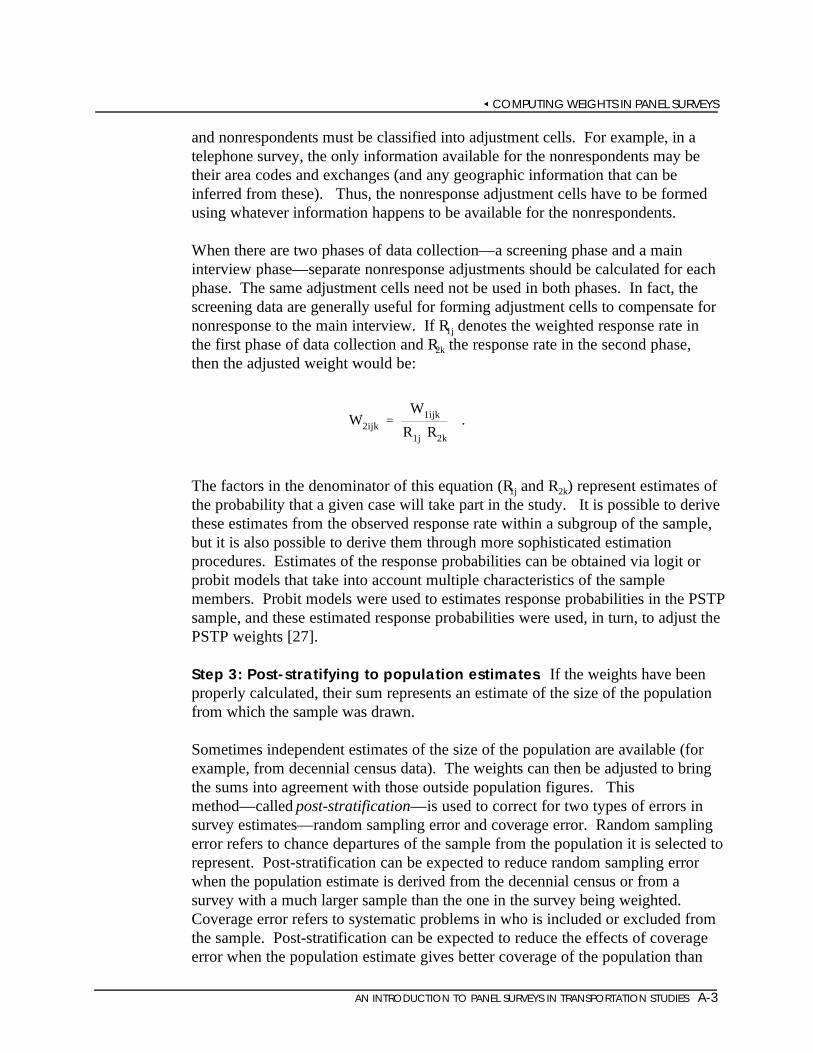
W2ijk

W1ijk

R1j R2k

.

COMPUTING WEIGHTS IN PANEL SURVEYS


and nonrespondents must be classified into adjustment cells. For example, in atelephone survey, the only information available for the nonrespondents may betheir area codes and exchanges (and any geographic information that can beinferred from these). Thus, the nonresponse adjustment cells have to be formedusing whatever information happens to be available for the nonrespondents.

When there are two phases of data collection—a screening phase and a maininterview phase—separate nonresponse adjustments should be calculated for eachphase. The same adjustment cells need not be used in both phases. In fact, thescreening data are generally useful for forming adjustment cells to compensate fornonresponse to the main interview. If R denotes the weighted response rate in1j

the first phase of data collection and R the response rate in the second phase,2k

then the adjusted weight would be:

The factors in the denominator of this equation (R and R ) represent estimates of1j 2k

the probability that a given case will take part in the study. It is possible to derivethese estimates from the observed response rate within a subgroup of the sample,but it is also possible to derive them through more sophisticated estimationprocedures. Estimates of the response probabilities can be obtained via logit orprobit models that take into account multiple characteristics of the samplemembers. Probit models were used to estimates response probabilities in the PSTPsample, and these estimated response probabilities were used, in turn, to adjust thePSTP weights [27].

Step 3: Post-stratifying to population estimates. If the weights have beenproperly calculated, their sum represents an estimate of the size of the populationfrom which the sample was drawn.

Sometimes independent estimates of the size of the population are available (forexample, from decennial census data). The weights can then be adjusted to bringthe sums into agreement with those outside population figures. Thismethod—called post-stratification—is used to correct for two types of errors insurvey estimates—random sampling error and coverage error. Random samplingerror refers to chance departures of the sample from the population it is selected torepresent. Post-stratification can be expected to reduce random sampling errorwhen the population estimate is derived from the decennial census or from asurvey with a much larger sample than the one in the survey being weighted. Coverage error refers to systematic problems in who is included or excluded fromthe sample. Post-stratification can be expected to reduce the effects of coverageerror when the population estimate gives better coverage of the population than

W3ij W2ij

Nj

W2ij

.

APPENDIX


the travel survey sample does. For example, if a telephone survey was used tocollect the data, the sample will necessarily exclude households withouttelephones. The two most commonly used sources of figures for post-stratificationare the decennial census and the Current Population Survey; these are thought toachieve much higher levels of coverage of the general population than othersurveys. The PSTP weights, for example, were adjusted to agree with the PublicUse Microdata Set (PUMS), an extract from the decennial census data [27].

Post-stratification involves comparing the sum of the weights (i.e., W) for a given2

subgroup with the population estimate for that group. For example, the PSTPweights were adjusted to agree with the PUMS totals for income-household size-number of vehicle groupings within each county. The post-stratificationadjustment is calculated by multiplying the current weight for cases in a subgroup,say subgroup j, by the ratio between the population estimate for that subgroup

(N ) and the sum of the weights for sample cases in that subgroup:j

The adjustment cells are typically defined in terms of areas (such as townships) andone or more demographic variables (such as household size).

Population figures for poststratification adjustments (the values for N in thej

equation) can be obtained from decennial census data, the CPS, or other CensusBureau estimates. Which source to use will depend on how recent the data are,whether they are based on sufficient sample sizes (in the case of the CPS), andwhether they provide appropriate grouping variables.

In general, both household-level and person-level weights can be calculated. Bothsets of weights can incorporate nonresponse and post-stratification adjustments(and different adjustment cells can be used in developing weights for householdsand persons).

A.2 DEVELOPING PANEL WEIGHTS

Step 1: Defining longitudinal households for weighting purposes. Onepractical approach to defining longitudinal households is to continue to treat as ahousehold all the persons who made up the household at the time of the first waveof data collection, regardless of what other changes that household subsequentlyundergoes. That is, each household is a treated a collection of persons and thelongitudinal weight is applied to this collection of persons even if they no longerlive together. For instance, if a couple divorced after the initial wave of datacollection, the longitudinal household weight would still be attached to both of the

W1i

W3i

Prri

.

COMPUTING WEIGHTS IN PANEL SURVEYS


households they now form. (Of course, analysts might want to take into accountthat this “household” now encompasses two separate residences, each of whichmay include other persons.) Although this approach has some obvious drawbacks,it is preferable to the main alternatives discussed in the statistical literature (forexample, restricting the analysis to intact households) and we recommend that it beadopted in travel panel surveys.

Step 2: Developing longitudinal base weights. Having defined longitudinalhouseholds, the next step in creating a longitudinal weight is to calculate a baseweight, reflecting the household’s selection probability. Generally, the householdsretained for follow-up in subsequent waves of the panel are drawn from the sampleof responding households in the first wave. Sometimes all Wave 1 respondents areincluded in the sample for Wave 2; in other cases, only a subsample is retained forfollow-up. When the sample for later waves is drawn from Wave 1 respondents,the base panel weight (W ) can be computed by dividing the final Wave 1p1

household weight by the probability of retention for later waves:

Since this initial weight is based on the final Wave 1 weight, it incorporatescorrections for Wave 1 nonresponse and adjusts for any discrepancies between thecomposition of the Wave 1 subsample and the population from which it wasdrawn. If all Wave 1 respondents are retained for follow-up, the initial panelweight is simply the final Wave 1 weight.

If new units are added to the sample in later waves, they must also receive a panelweight. If the new households represent in-movers (that is, immigration to thestudy area) or other additions to the Wave 1 population (e.g., births, returns froman institution), then the procedures outlined for weighting the Wave 1 householdsapply to the households added in later rounds as well. The new cases represent anew component of the population, one that was not previously eligible forinclusion in the sample.

When the new households are added because of changes in the composition ofWave 1 households, the situation is more complicated. Members of sampledhouseholds in the initial wave of a panel survey are sometimes referred to as “key”members of the sample. Other persons who join the households of key membersafter the initial wave but who were part of eligible population at the time of thefirst wave of the study are referred to as “non-key” members of the sample. Ourrecommended definition of a longitudinal household implies that data should becollected for key members in subsequent waves even if they move out of the

W2ij

W1i

Rj

.

APPENDIX


household that was sampled initially. For weighting purposes, these personsremain linked to their Wave 1 households. However, data should also be collectedfor non-key members while they are part of a household containing a key member;the data for non-key members can be used understand the context of the responsesof the key members [28].

All key members of the sample constitute the core sample for person-levelanalyses, both cross-sectional and longitudinal. Non-key members are included inperson-level analyses only in those waves when they were members of a householdthat included a key member of the panel survey. An alternative to the abovemethodology is to include only key members in all person-level analyses as done inthe National Medical Expenditure Survey (NMES) [28].

Step 3: Compensating for nonresponse. Once a longitudinal household hasbeen defined for weighting purposes, it is necessary to develop rules for classifyingthe household as a panel respondent or nonrespondent. The simplest rule is toclassify a household as a panel respondent if it provides the necessary data in eachwave. For example, in a three-wave survey, households would be classified asrespondents if they completed data collection in all three waves. All otherhouseholds would be treated as nonrespondents. The base weights of theresponding households can then be adjusted by the weighted response rate (that is,the weighted proportion of households that completed all three waves of datacollection):

This definition of respondents would produce a single set of longitudinal weightsfor all three waves. However, the definition may be too stringent for somepurposes. For example, an analyst may be interested only in data from the initialand most recent waves of data collection. For that purpose, it may be useful totreat households that completed those two waves of data collection asrespondents, even if they failed to take part in some intervening wave. Thisdefinition would produce a set of pairwise weights for the first and most recentwaves. Pairwise weights for the second and third waves could be generated in thesame way.

AN INTRODUCTION TO PANEL SURVEYS IN TRANSPORTATION STUDIES R-1

REFERENCES

1. Stopher, P.R. & Metcalf, H. (1996). Methods for Household TravelSurveys: A Synthesis of Highway Practice. Washington, DC: NationalAcademy Press.

2. Pendyala, R.M. & Pas, E.I. (1997). Multiday and multiperiod data for traveldemand analysis and modeling. Resource paper prepared for Workshop 5 ofTransport Surveys: Raising the Standard, International Conference onTransport Survey Quality and Innovation, Grainau, Germany, May 24-30.

3. Kitamura, R. (1990). Panel analysis in transportation planning: An overview.Transportation Research, 24A(6), 401-415.

4. Kitamura, R. (1987). Regularity and irreversibility of weekly travel behavior.

Transportation, 14, 227-251.

5. Goodwin, P.B. (1992). Panel analysis of travel behavior; some empiricalfindings. In T. Golob, R. Kitamura, and L. Long (eds.), Panels forTransportation Planning: Methods and Applications. Norwell, MA:Kluwer Academic Publishers.

6. Bradley, M. (1992). A practical comparison of modeling approaches forpanel data. In T. Golob, R. Kitamura, and L. Long (eds.), Panels forTransportation Planning: Methods and Applications. Norwell, MA: KluwerAcademic Publishers.

7. Baanders, A., De Boer, R.H., & Kroes, E.P. (1989). Impact of a newrailway line on travel patterns: The Flevo line in the Netherlands. PTRC17th Summer Annual Meeting; Proceedings of Seminar D, Brighton.

8. Supernak, J. (1992). Experiences with San Diego I-15 carpool lanes panel. InT. Golob, R. Kitamura, and L. Long (eds.), Panels for TransportationPlanning: Methods and Applications. Norwell, MA: Kluwer AcademicPublishers.

9. Smart, H. E.(1984). The dynamics of change - applications of the PanelTechnique to transportation surveys in Tyne and Wear. Traffic Engineeringand Control, 25, 595-598.

10. Kish, L. (1965). Survey Sampling. New York: John Wiley & Sons. Ltd.

REFERENCES

R-2 AN INTRODUCTION TO PANEL SURVEYS IN TRANSPORTATION STUDIES

11. Lawton, T.K., & Pas, E.I. (1996). Resource Paper, Survey MethodologiesWorkshop. In Proceedings, Conference on Household Travel Surveys: NewConcepts and Research Needs. Conference Proceedings No. 10,Transportation Restack Board, Washington, DC.

12. Goulias, K., Pendyala, R. & Kitamura, R. (1992). Updating a panel surveyquestionnaire. In Ampt, E., Richardson, A., Meyburg, A. (eds.) SelectedReadings in Transport Survey Methodology. Melbourne, Australia: Eucalyptus Press, 209-245.

13. McCormick, M., Butler, D. & Singh, R. (1992). Investigating time in sampleeffect for the Survey of Income and Program Participation. Paper presentedat the Joint Statistical Meetings in Boston, MA, August.

14. Kalton, G. & Miller, M. (1991). The seam effect with social security incomein the Survey of Income and Program Participation. Journal of OfficialStatistics, 7(2), 235-245.

15. Neter, J. & Wakesberg, J. (1964). A study of response errors inexpenditures data from household surveys. Journal of the AmericanStatistical Association, 59, 18-55.

16. Bailar, B. (1975). The effects of rotation group bias on estimates from panelsurveys. Journal of the American Statistical Association, 70(349),23-30.

17. Meurs, H., van Wissen, L., & Wisser, J. (1989). Measurement biases inpanel data. Transportation, 16, 175-194.

18. Golob, T.F., & Meurs, H. (1986). Biases in response over time in a seven-day travel diary. Transportation, 13, 163-181.

19. Pas, E.I, & Sundar, S. (1995). Intrapersonal variability in daily urban travelbehavior. Some additional evidence. Transportation, 22, 135-150.

20. U.S. Department of Commerce. (1992). Bureau of the Census. 1990 Censusof Population and Housing . Technical Documentation. Summary Tape File3 on CD-ROM.

21. Murakami, E., & Watterson, W. (1990). The Puget Sound TransportationPanel after two waves. Transportation, 19, 141-158.

REFERENCES

AN INTRODUCTION TO PANEL SURVEYS IN TRANSPORTATION STUDIES R-3

22. Meurs, H., & Ridder, G. (1997). Attrition and response effects in the DutchMobility Panel. In T. Golob, R. Kitamura, and L. Long (eds.), Panels forTransportation Planning: Methods and Applications. Kluwer AcademicPublishers, Norwell, M.A.

23. U.S. Department of Commerce (1978). Bureau of the Census. TechnicalPaper 40. The Current Population Survey: Design and Methodology.

24. The Ohio State University (1995). Center for Human Resource Research..National Longitudinal Survey Users’ Guide 1995.

25. Cochran, W.G. (1977). Sampling Techniques. New York: John Wiley &Sons.

26. Zimowski, M.F., Tourangeau, R., Ghadialy, R., & Pedlow, S. (1997).Nonresponse in Household Travel Surveys. Washington, DC: U.S.Department of Transportation. Federal Highway Administration

27. Goulias, K., & Ma, J. (1996). Analysis of Longitudinal Data From thePuget Sound Transportation Panel. Task D: Development and Performanceof Sample Weights for PSTP. Washington, DC: U.S. Department ofTransportation, Federal Highway Administration.

28. Cohen, S.B. (1990). Estimation concerns for family level analysis in NationalPanel Surveys. Proceedings of the Section on Survey Research Methods. American Statistical Association, 141-146.

AN INTRODUCTION TO PANEL SURVEYS IN TRANSPORTATION STUDIES S-1

SUGGESTED READINGS

Golob, J. M., Screurs, L. J. M., & Smit, J. G. (1986). The design and policyapplications of a panel for studying changes in mobility over time. In BehavioralResearch for Transport Policy. Utrecht, The Netherlands: VNU Science Press.

Goodwin, P. B. (1997). Have panel surveys told us anything new? In T. Golob,R. Kitamura, and L. Long (eds.), Panels for Transportation Planning: Methodsand Applications. Kluwer Norwell, MA: Academic Publishers.

Goulias, K., & Kitamura, R. (1997). A dynamic microsimulation model system forregional travel demand forecasting. In T. Golob, R. Kitamura, and L. Long (eds.), Panels for Transportation Planning: Methods and Applications. KluwerNorwell, MA: Academic Publishers.

Goulias, K., & Ma, J. (1996). Analysis of Longitudinal Data from the PugetSound Transportation Panel. Task C: Past Uses of PSTP Databases . U.S.D.O.T. Federal Highway Administration.

Goulias, K., & Ma, J. (1996). Analysis of Longitudinal Data from the PugetSound Transportation Panel. Task F: Cross Section and Dynamic Analysis ofActivity and Travel Patterns in PSTP. U.S. D.O.T. Federal HighwayAdministration

Hensher, D. A. (1985). Longitudinal surveys in transport: an assessment. In E.Ampt, A. Richardson, and W. Brog (eds.), New Survey Methods in Transport.Utrecht, The Netherlands: VNU Science Press.

Kasprzyk, D., Duncan, G., Kalton, G., & Singh, M. P. (1989). Panel Surveys. New York: J. W. Wiley and Sons, Inc.

Kitamura, R., & Bovy, P. H. L. (1987). Analysis of attrition biases and tripreporting errors for panel data. Transportation Research, 21A, 287-302.

Kitamura, R. (1990). Panel analysis in transportation planning: An overview. Transportation Research, 24A, 401-415.

Murakami, E., & Ulberg, C. (1997). The Puget Sound Transportation Panel. In T.Golob, R. Kitamura, and L. Long (eds.), Panels for Transportation Planning:Methods and Applications. Kluwer Norwell, MA: Academic Publishers.

Murakami, E. & Watterson, W. (1990). The Puget Sound Transportation Panelafter two waves. Transportation, 19, 141-158.

SUGGESTED READINGS

S-2 AN INTRODUCTION TO PANEL SURVEYS IN TRANSPORTATION STUDIES

Pendyala, R., & Kitamura, R. (1997). Weighting methods for attrition in choice-based panels. In T. Golob, R. Kitamura, and L. Long (eds.), Panels forTransportation Planning: Methods and Applications. Kluwer Norwell, MA:Academic Publishers.

Pol van de, F. (1987). Panel sampling designs. In Analyses of Panel Data, Proceedings of the Round Table Conference on the Longitudinal Travel Study,Projectbureau Integrale Verkeers- en Vervoersstudies, Ministrie van Verkeer enWaterstaat. The Hague, The Netherlands.

Richardson, A.J., Ampt, E.S., & Meyburg, A.H. (1995). Survey Methods forTransport Planning. Parkville, Vic: Eucalyptus Press.

AN INTRODUCTION TO PANEL SURVEYS IN TRANSPORTATION STUDIES G-1

GLOSSARY OF TERMS

ADJUSTED WEIGHTS: See nonresponse weighting.

CALIBRATION EXPERIMENT: When old and new versions of a survey instrument areadministered to different portions of the sample to assess the impact of changes in thequestions on responses.

COHORT: A group of individuals within a population who have experienced the same life eventduring some specified period in time. Cohort is usually defined by year or period of birth,but it may be used to refer to the timing of any number of other life events, such as year ofretirement or year of marriage.

CONDITIONING: See time-in-sample effects.

CPS: Current Population Survey.

DNMP: Dutch National Mobility Panel.

FIELD PERIOD: The time period during which survey data are collected from the respondents.

HOUSEHOLD: The U.S. Bureau of the Census defines a household as all persons who occupy thesame housing unit. A household may consist of a family, one person living alone, two ormore families living together, or any other group of related or unrelated persons whoshare living arrangements.

HOUSING UNIT: The U.S. Bureau of the Census defines a housing unit as a house, apartment,mobile home, group of rooms, or single room that is occupied (or if vacant, is intended foroccupancy) as separate living quarters. To qualify as a housing unit, the occupants mustlive and eat separately from any other persons in the building and have direct access fromthe outside of the building or through a common hall.

INCENTIVE: A monetary or nonmonetary gift or payment offered to sample members in an effortto gain their cooperation.

LOCATING LETTER: A letter sent by mail to the respondents in advance of the next data collectionperiod in an effort to obtain updated addresses and telephone numbers before the nextround of data collection.

LONGITUDINAL WEIGHTS: Weights designed to be used in longitudinal analyses of data from apanel survey.

LONGITUDINAL PANEL DESIGNS: Designs that collect information on the same set of variablesfrom the same sample members at two or more points in time.

GLOSSARY OF TERMS

G-2 AN INTRODUCTION TO PANEL SURVEYS IN TRANSPORTATION STUDIES

MODULE: An independent part of a questionnaire that covers a single subject or topic of interest.

NLSY: National Longitudinal Survey of Youth.

NMES: National Medical Expenditure Survey.

NONRESPONSE: Failure of the survey to obtain the desired information from eligible samplemembers.

NONRESPONSE WEIGHTING: Postsampling statistical adjustment to partially compensate forpossible nonresponse error. Statistical weighting to compensate for nonresponse isdifferent from the postsampling weighting that is routinely performed to adjust for unequalprobabilities of selection.

ONE-TIME CROSS-SECTIONAL DESIGNS: Designs in which sample members are asked tocomplete a survey once.

PANEL ATTRITION: Failure of first-wave respondents to complete the survey in subsequentrounds of a panel survey.

PANEL DESIGNS: Designs that collect repeated measurements on the same sample of individualsor households over time.

PANEL FATIGUE: See time-in-sample effects.

POST-STRATIFICATION: When weights are adjusted to agree with independent populationestimates. Post-stratification compensates for deviations between the distribution ofcharacteristics in the sample and the target population.

PSTP: Puget Sound Transportation Panel.

REPEATED CROSS-SECTIONAL DESIGN: Designs that collect measurements on a population overtime by repeating the same survey on two or more occasions. During each time period, aseparate but comparable sample of units is drawn from the population.

RESPONSE RATE: A measure of a survey’s level of success in obtaining the desired measurementsfrom all eligible units in the sample; the number of respondents divided by the totalnumber of eligible units in the sample.

RETENTION RATES: The proportion of respondents from the first wave who complete laterwaves of data collection in a panel survey.

ROTATION GROUP BIAS: See time-in-sample effects.

GLOSSARY OF TERMS

AN INTRODUCTION TO PANEL SURVEYS IN TRANSPORTATION STUDIES G-3

ROTATING PANEL DESIGNS (REVOLVING): A panel design that collects measurements on asample for some specified number of periods after which the sample is dropped from thesurvey and replaced with a new but comparable sample of units drawn from the currentpopulation.

ROTATION GROUP: A sample of units drawn from the population at the same time and followingthe same schedule of data collection in a rotating panel design.

RDD: Random Digit Dialing. Techniques that form samples by adding random digits to thetelephone prefixes that fall within the sampling area so as to include both listed (published)and unlisted numbers in the sample.

SAQ: Self-administered questionnaire. A questionnaire that is completed by the sample memberwithout the assistance of an interviewer. Respondents to self-administered questionnairesare asked to read the questions and record the answers on their own.

SAMPLING UNIT: An element in a sampling frame from which a survey sample is drawn.

SEAM EFFECTS: Apparent increase in the number of changes across rounds of a survey ascompared to the number observed within a round.

TIME SERIES DESIGN: A design that collects a series of repeated measurements over a relativelylarge number of points in time.

TIME-IN-SAMPLE EFFECTS: Effects of prior reporting on reporting in subsequent waves of datacollection. Conditioning and fatigue refer to reduced levels of reporting across waves. Rotation bias refers to differences across rotation groups related to their time in thesample.

WAVE: A distinct occasion when data are collected in a panel survey. Also referred to as a roundof data collection.

WEIGHTED RESPONSE RATE: A response rate that is calculated using the inverse of the selectionprobabilities as the weight. The weighted response rate is an estimate of the proportion ofthe target population represented by the respondents to the survey.

Roger Tourangeau, Michele Zimowski, Rashna … · Roger Tourangeau, Michele Zimowski, and ... Peter...

Documents

Transcript of Roger Tourangeau, Michele Zimowski, Rashna … · Roger Tourangeau, Michele Zimowski, and ... Peter...