RODOS migration - resy5.iket.kit.edu€¦ · considered in the modelling of atmospheric dispersion...

Description of the Atmospheric Dispersion Model ATSTEP

Version RODOS PV 6.0 Final

D R A F T V e r s i o n 2 . 0

R O D OS DECISION SUPPORT FOR NUCLEAR EMERGENCIES

R E P O R T

RODOS(RA2)-TN(04)-03

RODOS migration contract


Draft] 20.03.03 2


Draft] 20.03.03 3

Description of the Atmosperic Dispersion Model ATSTEP - Version RODOS PV 6.0 Patch07 RODOS(RA2)-TN(04)-03

Jürgen Päsler-Sauer Forschungszentrum Karlsruhe GmbH Institut für Kern- und Energietechnik

Postfach 3640 D-76021 Karlsruhe

Email: [email protected]

Draft, 30 Juli 2007


Draft] 20.03.03 4


Draft] 20.03.03 5

Management Summary

This report describes the atmospheric dispersion and deposition model ATSTEP. The basic mathematical formulas used in the model are given and their physical meaning and model approximations are explained and illustrated. The use of additional models in ATSTEP for plume rise, deposition and depletion, daughter nuclide build-up, and gamma radiation is described. Furthermore the internal structure of the ATSTEP code and the use of the SUBROUTINE ATSTEP in RODOS diagnosis- and prognosis modules is shown. Subroutines used together with ATSTEP are described.

ATSTEP is a Gaussian puff model for distances up to 50 km. It was developed especially for quick simulation calculations in the case of accidental releases of airborne radioactive contaminants. In RODOS 6.0 the model can calculate real-time diagnoses of the radiological situation during or after a release without limitation of duration and interactive dispersion prognoses/episodes for up to 47 days. The radiological situation is described by the following results calculated with ATSTEP: the concentration in the air near ground (instantaneous and time-integrated), the contamination of ground surface (dry and wet), and the gamma radiation from ground and from the radioactive cloud. These results are presented as time dependent, nuclide specific fields in the whole calculation area in the environment of the source of the release. In ATSTEP the following phenomena are considered in the modelling of atmospheric dispersion and the radiological situation: time dependent meteorology (meteorological tower- or SODAR data, forecast data, inhomogeneous wind fields), time dependent nuclide-group specific release rates, thermal energy and rise of the puffs released, dry and wet deposition and corresponding depletion of the cloud, gamma radiation from cloud and from ground, radioactive decay and (in two special cases) build-up of daughter nuclides, and potential doses. ATSTEP’s areas of application are accidental releases from nuclear installations, radioactive releases from transport accidents including fire, and from radiological dispersal devices (dirty bombs).

Different to classic puff models in ATSTEP no instantaneous puffs but time-integrated elongated puffs are released. The transport of each elongated puff is achieved by two trajectories attached to both ends of the puff. As these pairs of trajectories follow the inhomogeneous and variable 2D-wind fields step by step, also the elongated puffs perform all the necessary changes in position, shape, and orientation, like stretching, rotations, shrinking, and sideways drift.

Because of the large size of the elongated puffs the plume can be represented by a relatively small number of puffs. Correspondingly the number of time steps needed for the simulation of the release and the transport is small. The elongated puff approximation reduces the computing time of the model code, so that during less than 10 minutes real-time a complete dispersion and contamination prognosis can be performed with releases over several hours. Nevertheless the spatial and temporal resolution of the results is fully sufficient for the applications in the RODOS system.

The work described in this report has been performed with support of the European Commission under the contract “Migration of RODOS to practical applicability for supporting decisions in operational emergency response to nuclear accidents” contract RODOS Migration, contract no. FIKR-CT-2000-00077.


Draft] 20.03.03 6


Draft] 20.03.03 7

Table of Contents

1 Model description .......................................................................................................................................................7

1.1 Advection and Diffusion in ATSTEP .................................................................................................................7 1.1.1 Time steps and puffs ...................................................................................................................................7 1.1.2 puff trajectories ...........................................................................................................................................9 1.1.3 puff time-integral calculation with sideways drift of puffs .......................................................................10 1.1.4 Transport in inhomogeneous, variable windfields ....................................................................................12 1.1.5 Dispersion parameters ...............................................................................................................................12 1.1.6 Reflection at ground surface and lid on top of mixing layer.....................................................................14 1.1.7 Vertical wind profile and concentration weighted transport velocity vector ............................................14 1.1.8 Puff rise by thermal energy and initial momentum...................................................................................15 1.1.9 Dirty Bomb and Transport Accidents .......................................................................................................15

1.2 Deposition to surfaces and depletion of the cloud ............................................................................................17 1.2.1 Dry deposition: deposition velocities........................................................................................................17 1.2.2 Wet deposition: Washout ..........................................................................................................................18 1.2.3 Deposition depending on location and puff depletion ..............................................................................19

1.3 Radioactive decay and build-up of daughter nuclides ......................................................................................20 1.4 Gamma radiation fields .....................................................................................................................................21

1.4.1 Cloud gamma radiation .............................................................................................................................21 1.4.2 Ground gamma radiation...........................................................................................................................22

2 The ATSTEP-Code...................................................................................................................................................23 2.1 ATSTEP in different RODOS ASY modules ...................................................................................................23

2.1.1 ATSTEP in the prognosis module ALSMCprogn.....................................................................................23 2.1.2 ATSTEP in the interactive module QUICKPROGNO .............................................................................23 2.1.3 ATSTEP in the diagnosis module Atstepdiagn.........................................................................................23

2.2 Inner structure of the ATSTEP code.................................................................................................................24 2.3 Subsequent programmes of ATSTEP ...............................................................................................................26

3 References.................................................................................................................................................................29

1 Model description

1.1 Advection and Diffusion in ATSTEP

1.1.1 Time steps and puffs

In ATSTEP the duration T[s] of a release step equals the duration of the advection step. The release rate QR[Bq/s] at the source and the wind velocity and direction u[m/s] and θ[0] are assumed to be constant during the time step. After each time step of duration T a puff is released from the source with a puff length uT[m] and an puff axis direction θ-1800..


Draft] 20.03.03 8

Fig. 1: Geometry for a puff release

The cross wind diffusion is modelled using horizontal and vertical Gaussian distributions normal to the puff axis; the corresponding sigma-parameters are σy and σz. They depend on the length co-ordinate x as in the Gaussian plume model. The longitudinal diffusion is modelled by error-functions with the parameter σx. Therefore the puff extends beyond the advection length uT (Fig. 2). The resulting concentration distribution of the puff equals the time-integral TIC(x,y,z)[Bq.s/m3] of a 3-dimensional Gaussian distribution χ0 (ellipsoidal puff), that was advected from the source to the distance uT and that was extended corresponding to the increase of the σ-parameters (Eq. 1 and 2).

(Eq. 1)

( )χ

π σ σ σ σ σ σ0 3

2 2 2

2

12

12

12

( , , ) exp exp expx y zQR x y z

x y z x y z= −

⎛⎝⎜

⎞⎠⎟

⎛

⎝⎜⎜

⎞

⎠⎟⎟ −

⎛

⎝⎜⎜

⎞

⎠⎟⎟

⎛

⎝⎜⎜

⎞

⎠⎟⎟ −

⎛⎝⎜

⎞⎠⎟

⎛

⎝⎜⎜

⎞

⎠⎟⎟ (Eq. 2)

The computation of the time-integral TIC leads to the function F(x), which is a superposition of error functions and models the length uT and the σx-diffusion of the puff..

uxFuTxerfxerf

udtutx

xxx

T

x

)(:222

121exp

21

2

0

=⎟⎟⎠

⎞⎜⎜⎝

⎛⎟⎟⎠

⎞⎜⎜⎝

⎛ −−⎟⎟

⎠

⎞⎜⎜⎝

⎛=⎟

⎟

⎠

⎞

⎜⎜

⎝

⎛⎟⎟⎠

⎞⎜⎜⎝

⎛ −−∫ σσσσπ

(Eq. 3)

Θ-180

N

S

W

x

y

E

h

u,wind

uT

x´

Θ

y´

σz σy

σx

∫ −−=T

dthzyutxzyxTIC0

0 ),,(),,( χ


Draft] 20.03.03 9

The complete concentration distribution of a puff (without ground surface and top of mixing layer reflection) is then given by:

⎟⎟

⎠

⎞

⎜⎜

⎝

⎛⎟⎟⎠

⎞⎜⎜⎝

⎛ −−⋅⎟

⎟

⎠

⎞

⎜⎜

⎝

⎛

⎟⎟⎠

⎞⎜⎜⎝

⎛−⋅⋅=

22

21exp

21exp)(

2),,(

zyzy

hzyxFuQRzyx

σσσσπχ (Eq. 4)

A typical concentration distribution along the puff axis is shown in Fig. 2 a. The square with length uT corresponds to the puff‘s length without diffusion in x-direction, i.e. the plume segment‘s length. The slope of the curve in the middle of the picture results from the increasing dilution of the concentration due to the σ-parameters σy and σz. The tails of the curve result from the error-functions (Eq. 3) and represent physically the downwind and upwind diffusion along the puff axis. In this way the puff‘s concentration field is calculated from a plume segment‘s field by smearing it out along its axis in a mass conserving manner. Fig. 2 b shows the cross axis Gaussian distribution.

Fig. 2: Concentration curves on the puff axis and on the lateral y axis

1.1.2 puff trajectories

For determining the location, the orientation, and the spread of a puff during the transport in a variable wind field, two trajectories are calculated for each puff. They start at the source location and follow the movements of the start- and end-points of the puff axes in each time step during the atmospheric dispersion calculation. After each time step the change of orientation and length of the puff axis is determined corresponding to the local transport vectors uA(t) and uE(t) at the starting point A and the end point E of the puff i (see 2.1.7). The construction of the puff trajectories is carried out like shown in Fig.3 and results in 2n polygon curves in a plain layer at release height if n puffs were released. Because ATSTEP does not use 3-dimensional wind fields, but 2-dimensional wind fields plus vertical profiles, the trajectories are 2-dimensional curves in the height layer of the puff axis, except for the case of thermal puff rise (see 2.1.8).

conc. conc.

x y uT

σy

a b


Draft] 20.03.03 10

Fig. 3: Puff transport by a pair of trajectories

1.1.3 puff time-integral calculation with sideways drift of puffs

If wind fields depend on time generally the puff’s transport direction will not be parallel to the puff’s axis (sideways drift, Fig.3). Figure 4 shows the approximation that is used in ATSTEP to calculate time-integral of the air concentration if puff transport is sideways. The time-integral of the puff i during the step from t to t+T is shown by the grey shaded area. Because of the diffusion it is more extended than the area covered by the puff axis (the trapeze with wave pattern), and is mathematically described by a two-dimensional function F(x,y) like in Eq. 3

Fig. 4: Time-integral of a puff after one time step T

time t Trajectory 1

time t + T

Trajectory 2

uA(t)

uE(t)

x y puff i, time t

puff i, time t + T

Area covered by axis

puff i, time step-integral from t to t+T

Trajectory 1

Trajectory 2


Draft] 20.03.03 11

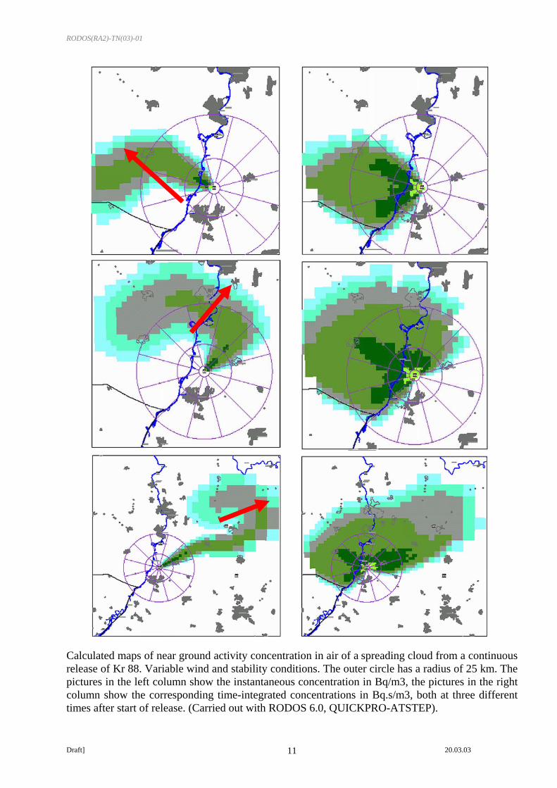
Calculated maps of near ground activity concentration in air of a spreading cloud from a continuous release of Kr 88. Variable wind and stability conditions. The outer circle has a radius of 25 km. The pictures in the left column show the instantaneous concentration in Bq/m3, the pictures in the right column show the corresponding time-integrated concentrations in Bq.s/m3, both at three different times after start of release. (Carried out with RODOS 6.0, QUICKPRO-ATSTEP).


Draft] 20.03.03 12

1.1.4 Transport in inhomogeneous, variable windfields

The most general case is a spatially inhomogeneous, time dependent windfield. In this case the orientations and the lengths of the puffs change during the time step from t to t+T. The growth of the puffs by diffusion is taken into account by increasing the size of their σ-parameters corresponding to the increase of their total travelled distances.

Fig. 5: Transport in inhomogeneous, variable windfield

1.1.5 Dispersion parameters

The modelling of turbulent diffusion in ATSTEP is parameterised by using diffusion parameters either depending on travelled distance (Eq. 5) or on travelled time(Eq. 6):

yqyy xp ⋅=σ

zqzz xp ⋅=σ , yx oder σσσ =∝ Θ (Eq.5)

( )tyy σσ = ( )σ σz z t= (Eq.6)

σ-parameters depending on travelled distance

In the case of dispersion parameters depending on travelled distance (Eq.5) there are 2 classes of roughness length (z0 = 0.5 -1 m and z0 = 1 -1.5 m). The dispersion parameters are defined by sets of dispersion coefficients py, qy and pz, qz for σy and σz which are derived from tracer dispersion measurements. The Mol-SCK-CEN parameters set [1] corresponds to lower roughness length (rural, small houses, open or with trees), the Karlsruhe-Jülich set[2] corresponds to higher roughness (urban, with high buildings or forest). Both sets have 6 Pasquill-Gifford diffusion categories. The Karlsruhe-Jülich set is additionally defined for 3 different release heights: 50m, 100m und 180m.

time t + T

time t


Draft] 20.03.03 13

The Karlsruhe-Jülich and Mol σy(x) parameters generally are valid up to about Xvalid=10 km of travelled distance. In case of the Karlsruhe-Jülich parameters, release heights above 75 m, and strong convective or very stable conditions (PG-categories A, B, or F), the corresponding Xvalid is reduced to 2000, 4000, or 4000 m. Beyond Xvalid the following σy(x) parameterization is used in ATSTEP corresponding to Briggs[4]:

xaXvalidxy ⋅=≥ )('σ (Eq.7)

Here a is defined such that σy(x) changes smoothly into σ’y(x) at x=Xvalid.

Diffusion along the axis of the puff is described by σx(x). At small distances σx is determined from the horizontal wind direction fluctuation σθ corresponding to the dominating small scale turbulence. At larger distances σx is derived from σy.

The variable x used in this paragraph means the straight line way travelled like in the Gaussian plume model. Instead of this the trajectory lengths are taken in ATSTEP.

In ATSTEP all σ(x) parameters are calculated by adding their differential increase during each time step, so that in each time step from t1 to t2 a change of the diffusion category is possible:

))()(())(())(( 1212qq txtxptxtx −⋅+= σσ (Eq.8)

The σ-parameters σ(x(t2)) at the trajectory point x at time t2 are calculated from the parameters at the point x(t1) during the step from t1 to t2, by adding the difference term in Eq. 8. The dispersion coefficients p and q are chosen corresponding to the actual diffusion category, puff height, and to the local roughness length defined by the land use. In case of variable land use under the flying puff therefore both Karlsruhe-Jülich and Mol parameters may contribute to its time-integrated plume.

Eq. 8 shows that growth of the σ(x) parameters only can be achieved by a variation of x in time: (x(t2) =/= x(t1). Therefore no turbulent broadening of the puffs would be possible during zero wind speed. In case of a local zero wind speed ATSTEP assumes a very small non-zero wind speed of 0.1 m/s and a zigzag-direction, causing the puff’s head and/or end jitter to and fro a bit with the time steps. So the puff can grow though it is effectively not moving.

σ-parameters depending on travelled time

The time dependent dispersion parameters (Eq.6) are the sigma parameters σS of the spectral turbulence model which was chosen as a suitable common German-French model by the German French Commission (GFC) [3]. The variable t means the travelled time of each respective puff. Therefore a turbulent broadening of the puff is also possible during zero wind speed without change of puff location. The GFC-σS parameters continuously consider wind speed, height of the puffs, roughness length, Monin Obuchov length, and the friction velocity. The σS parameters are calculated outside ATSTEP with the new meteorological data during each time step and are stored in a table with travelling times of 0-10000 seconds. During the dispersion calculation step in ATSTEP the sigma parameter values σxyzE(t) and σxyzA(t) at both puff ends are taken from the table and interpolated corresponding to their travel times for all released puffs.


Draft] 20.03.03 14

1.1.6 Reflection at ground surface and lid on top of mixing layer

In the Gaussian modelling of the vertical concentration profile total reflection of the concentration at the ground surface and the top of the mixing layer are assumed. The reflection at ground surface enhances the air concentration close to the surface by a factor of 2. The additional reflection at the top of the mixing layer causes the air contamination to get trapped in the mixing layer. Turbulent vertical mixing finally generates a uniform profile of the vertical contamination that is inversely proportional to the mixing height hmix. In the model this is approximated by replacing σz(x) by ~0.8 * hmix in Eq. 5 , if σz(x) exceeds 80% of the mixing height (Eq. 8):

σπz mix mixx h h( ) .≥ ⋅ = ⋅2

08 (Eq. 9)

χπσ σ

( , , )( ) .

( ) expx yQ

x h uF x

y

y mix y

00 8

12

2

=⋅ ⋅ ⋅

⋅ ⋅ −⎛

⎝⎜⎜

⎞

⎠⎟⎟

⎛

⎝⎜⎜

⎞

⎠⎟⎟ ⋅ (Eq. 10)

In a Gaussian puff model material of a puff can not penetrate the inversion lid of the mixing layer. Neither can a puff that has expanded vertically to a given mixing layer height during day time shrink to smaller heights if the mixing height comes down during night time. The vertical extension of a puff can only stay constant or grow. Therefore in the model each puff gets it's own history of mixing heights which can stay constant (if the real mixing height falls), or increase to a higher real mixing height.

1.1.7 Vertical wind profile and concentration weighted transport velocity vector

Wind speed and direction generally depend on height. The wind speed profile is generated in the meteorological pre-processor in the form of a power law (Eq. 11) from wind data measured at various heights. The directional shear profile is assumed to change linearly with height below 200 m. If there is only one measurement height a default power law profile is used for defining the wind at other heights. In this case no directional shear with height is assumed. The power law profile parameter (wind profile exponent WP) depends on diffusion category and roughness length z0:

u z u zz

zmm

WP

( ) ( )= ⋅⎛⎝⎜

⎞⎠⎟ (Eq. 11)

The resulting transport velocity vectors with which the head and the end of each puff are moved along their trajectories are not just equal to the wind vectors at puff axis height. This happens

because of the concentration profiles and wind profiles involved: The bottom parts of a concentration cloud move more slowly and into another direction than the top parts. Nevertheless each puff has to be transported as a whole using two effective transport velocities at the head and

the end of each puff. To determine the mass profile weighted transport velocity vectors the vertical profiles of concentration and of the wind vector are taken at 9 different levels of height. The

weighted sum over these height levels then leads to the effective transport velocities.


Draft] 20.03.03 15

1.1.8 Puff rise by thermal energy and initial momentum

If thermal energy or initial vertical momentum is released with a puff the rising phase and the final rise is considered in the form of a rising trajectory of this puff.

In the rise model first the relations of volume flux, exhaust velocity and temperature contained in the release data are transformed into a criterion for buoyancy or momentum dominated rise. Then the rise phase of either a thermal or a momentum release is calculated taking into account neutral, stable, and unstable atmospheric stratification, and the corresponding wind profile following the plume rise model of Briggs [5].

From this the final rise of the puff ∆hfin and the corresponding distance xfin is derived. The rising phase of the puff trajectory is then calculated as a x2/3-curve like in Fig. 6. The model does not allow for puffs penetrating the lid of the mixing layer.

Fig. 6: Trajectory of a puff with rise by thermal energy or initial vertical momentum

1.1.9 Dirty Bomb and Transport Accidents

Both cases have in common that they are not predictable at all. Location and time of release can be known only after the event. Assessed values of the source term, of released thermal power or mass of the explosive device, and local weather data can be used to start an interactive dispersion calculation with RODOS. A time step length of 10 minutes is default. A special module is used to assess the rise and initial size of the cloud of a dirty bomb, and special parameters are used to assess the rise of the plume resulting from a transport accident with fire.

x

z

Xfin

∆hfin


Draft] 20.03.03 16

Transport Accident

For the calculation of plume rise in case of a transport accident with a fuel fire the same module is used as in case of a release from a NPP. But there is a different interpretation of input parameters: the venting area is changed into the burning area of the fuel, the exhaust velocity is set to zero, and the heat power of the fire has to be assessed.

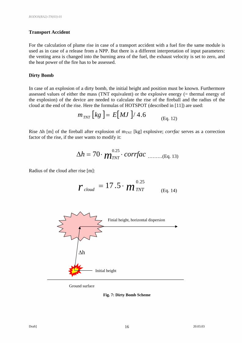
Dirty Bomb

In case of an explosion of a dirty bomb, the initial height and position must be known. Furthermore assessed values of either the mass (TNT equivalent) or the explosive energy (= thermal energy of the explosion) of the device are needed to calculate the rise of the fireball and the radius of the cloud at the end of the rise. Here the formulas of HOTSPOT (described in [11]) are used:

[ ] [ ] 6.4/MJEkgmTNT = (Eq. 12)

Rise ∆h [m] of the fireball after explosion of mTNT [kg] explosive; corrfac serves as a correction factor of the rise, if the user wants to modify it:

corrfach mTNT ⋅⋅=∆ 25.070 ………(Eq. 13)

Radius of the cloud after rise [m]:

mr TNTcloud

25.05.17 ⋅= (Eq. 14)

Fig. 7: Dirty Bomb Scheme

∆h

Initial height

Finial height, horizontal dispersion

Ground surface


Draft] 20.03.03 17

1.2 Deposition to surfaces and depletion of the cloud

In ATSTEP 4 groups of radioactive materials are distinguished according to their dry and wet deposition properties. These (deposition-) groups are:

• noble gases (neither dry nor wet deposition) • elementary iodine, i.e. airborne I2-vapor (dry and wet deposition) • organically bound iodine, e.g. Methyl Iodide CH3I (dry and wet deposition) • aerosols, i.e. radionuclides in aerosol form or bound to aerosols, e.g. aerosol iodine, metal oxides (dry and wet deposition)

1.2.1 Dry deposition: deposition velocities

The contamination of a surface in contaminated air can be characterised by the deposition velocity vd. It is defined as the ratio of the contamination rate dCd/dt of the surface and the nuclide concentration in the ambient air χ:

vms

dCdt

Bqm s

Bqm

C dt CTICd

dd

d⎡⎣⎢

⎤⎦⎥

=⎡⎣⎢

⎤⎦⎥

⎡⎣⎢

⎤⎦⎥

= =∫2 3χ χ (Eq. 15)

Correspondingly the ground contamination is calculated in ATSTEP during each time step from the time-integrated concentration in the air near ground and the deposition velocity. The deposition velocities of the deposition groups depend on the degree of vertical turbulent mixing of the air (atmospheric resistance) and on local surface properties (canopy resistance), which can be derived in a simplified manner from the land use. The deposition velocities are derived in this way in the Meteorological Preprocessor (MPP) using the DEPOSITION routines [6]. In the case of the interactive RODOS module QUICKPROGNO, as it works without the MP, the resistances and deposition velocities are calculated in the QUICKPROGNO-ATSTEP

The RODOS database contains land use information containing 5 classes:

• 1) Settlements, Urban or Industrial areas, 2) Pasture, 3) Agricultural areas, 4) Forest, 5) Water Attention: The standard surface type used in RODOS and ATSTEP is lawn. In ATSTEP ground contaminations are calculated exclusively assuming this surface type. This holds also for the calculation of ground gamma radiation and local gamma dose rates, i.e., location factors =1 are assumed. This does not imply that the plume is depleted corresponding to the surface type lawn. For depletion calculations the land use pattern under each puff is considered. An effective depletion is derived for each puff during each time step from the local deposition velocities in the area of the puff (1.2.3).

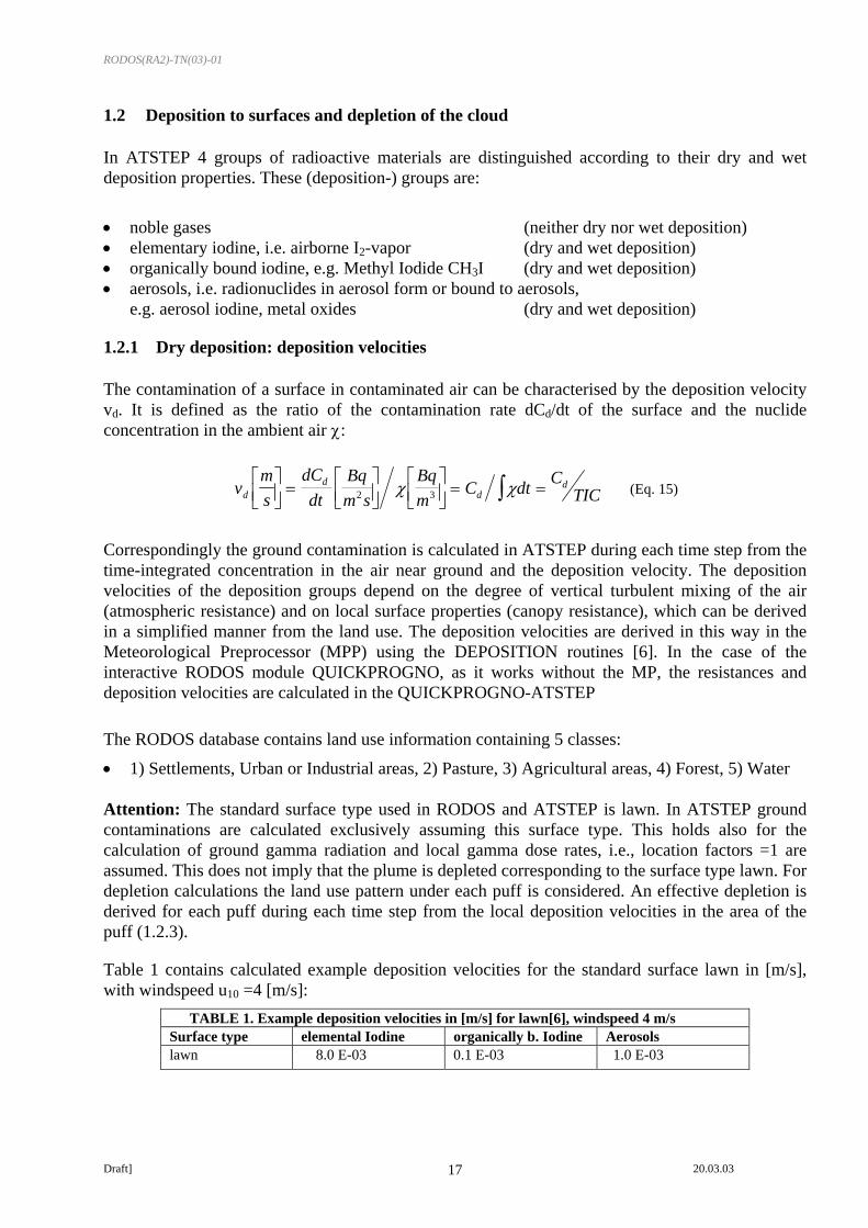
Table 1 contains calculated example deposition velocities for the standard surface lawn in [m/s], with windspeed u10 =4 [m/s]:

TABLE 1. Example deposition velocities in [m/s] for lawn[6], windspeed 4 m/s Surface type elemental Iodine organically b. Iodine Aerosols lawn 8.0 E-03 0.1 E-03 1.0 E-03


Draft] 20.03.03 18

Depletion, dry Due to mass conservation the material ∆Q taken from a puff during deposition corresponds to the surface contamination under the puff times the area ∆F covered:

[ ] [ ]∆ ∆ ∆ ∆Q Bq CBqm

F m v TIC x y m x yd d= −⎡⎣⎢

⎤⎦⎥

⋅ = − ⋅ ⋅22 1( , , ) (Eq. 16)

Integration of Eq. 16 gives the amount of material reduced by depletion of a vertically Gaussian puff during transport in x direction:

Q x Qvu x

hx

dxd

zx

x

z( ) exp

( ' )exp

( ' )'= ⋅ − ⋅ ⋅ ⋅

−⎛

⎝⎜

⎞

⎠⎟

⎛

⎝⎜⎜

⎞

⎠⎟⎟∫0

2

2

2 12

0π σ σ (Eq. 17)

The integral over the variable x’ is solved numerically, as long σz is still growing and depends on x, i.e. if there is no homogeneous vertical mixing of the puff.

1.2.2 Wet deposition: Washout

Wet deposition is calculated using a washout model with the parameter Λ[1/s]. The contamination Cw[Bq/m2] is the product of the washout constant Λ, the precipitation duration ∆t, and the integral of the vertical profile χ of the Gaussian puff:

C t dzw = ⋅ ⋅ ⋅∫Λ ∆ χ (Eq. 18)

The washout constant depends on the deposition group and the precipitation intensity I in [mm / h]:

[ ] [ ]Λ 1

1s

b

aI

mm h= ⋅

⎛⎝⎜

⎞⎠⎟/ (Eq. 19)

In table 2 the values of a and b for different deposition groups are given: TABLE 2. Parameters a and b for wet deposition [7]

deposition group a b noble gases 0 0 aerosols 8.0 E-5 0.8 elementary iodine 8.0 E-5 0.6 org. bound iodine 8.0 E-7 0.6


Draft] 20.03.03 19

Depletion, wet

The amount of material still in the puff after being washed out during the time t (or during transport in x direction with velocity u) is:

( ) ⎟⎠⎞

⎜⎝⎛ ⋅Λ−⋅=⋅Λ−⋅=

uxQtQxQ expexp)( 00 (Eq. 20)

It is assumed that the cloud is washed out homogeneously over its full depth.

1.2.3 Deposition depending on location and puff depletion

Generally deposition processes depend on local conditions. Local land use defines the kind of surfaces (agricultural use, canopy, etc.) and by this influences the dry deposition velocities (surface resistance). Additionally the local state of turbulence of the atmosphere influences the resistance against vertical transport (atmospheric resistance). In the case of wet deposition the local precipitation intensity a local value of the washout parameter Λ. The local values of the deposition parameters vD and Λ are defined as fields on the calculation grid, so that each grid cell has its own set of deposition parameters. Because the state of turbulence and precipitation can change this set is time dependent.

The concentration of the material staying in the depleted cloud after deposition is calculated assuming „source depletion“, i.e., the amount of material deposited from a puff onto a surface is taken from the puff as a whole, not only from the near to the surface parts of the puff‘s volume. Because a puff generally covers more than one grid cell with locally different deposition parameters during the advection step, but the puff can only be depleted as a whole, its depletion can only be calculated with effective, puff-averaged deposition parameters. The exact way to determine these effective parameters is to calculate the concentration weighted average of the vD- and Λ-values in all the grid cells under the puff.

Fig. 8: Grid cells covered by the puff during time step t1 to t2 a) constant 41 x 41 cells grid, b) non-uniform grid

Instead of this in ATSTEP the simple average over the grid cells with the highest concentrations of the puff, i.e. the grid cells within the σy-surrounding of the puff axis, is calculated. For this purpose rectangles with 2σy width are constructed around the puff axes before and after the transport step (at times t1 and t2). Then the grid cells situated inside these rectangles are determined, and the averages of the deposition parameters in these cells are calculated. These averages are used as effective deposition parameters for determining the depletion of the puff in the step from t1 to t2.

2σy

t1

t2 2σy

t1

t2 2σy


Draft] 20.03.03 20

1.3 Radioactive decay and build-up of daughter nuclides

Radioactive decay is calculated at each time step for all nuclides during dispersion and deposition and is considered in the output fields concentration in air, ground contamination, potential doses and dose rates.

During atmospheric dispersion and deposition of radionuclides radiologically important daughter nuclides can be produced in the cloud and on contaminated surfaces. Resulting transformations of the chemical form of the nuclides and changes of their deposition properties can lead to complex contamination patterns. A general modelling and code simulation of the build-up, the transport, and the decay of daughter nuclides during the dispersion and deposition calculations is not carried out in ATSTEP. Computer storage and computation times needed for that would exceed the desired level by far. In order not to neglect striking or radiologically important radionuclides in spite of this, some special nuclide specific modellings concerning build-up, deposition, and decay of daughter nuclides are installed. In RODOS-ATSTEP version 4.0 (July 2000), RODOS 5.0 (2003), and RODOS 6.0 (2004) the mother-daughter pairs of nuclides Te-132 and I-132, as well as Kr-88 and Rb-88 are taken into account.

Te-132 and I-132

If there is Te-132 in the calculated release the build-up of the daughter I-132 is considered. Because the Te-132 is released as an aerosol it is assumed that the daughter is an aerosol too and has the same deposition velocity. Dispersion, depletion, and deposition are the same for both nuclides so that the mother-daughter ratio in the air and on ground is only defined by radioactive build-up and decay. If there is I-132 already in the release, as a mixture of elementary, organically bound, and aerosol fractions, the mixing ratio is recalculated according to the additional quantity of the aerosol daughter iodine.

Kr-88 and Rb-88

If there is Kr-88 in the release the buil-up of the daughter Rb-88 is considered. Kr-88 is a noble gas and does not deposit. Its daughter Rb-88 is assumed to be an aerosol and therefore deposits. In the Kr-Rb-88 cloud the mother-daughter ratio is defined by the radioactive build-up and decay, as well as by depletion of the daughter. The ground surface contamination with Rb-88 is locally produced by deposition from the Kr-Rb-88 cloud and decays again according to the temporal distance from that deposition. If there is Rb-88 already in the release it decays according to the temporal distance from the start of the release.


Draft] 20.03.03 21

1.4 Gamma radiation fields

In ATSTEP nuclide specific and total gamma radiation fields are calculated. The fields are the gamma dose rates in [mSv/h] and doses in [mSv] from the contaminated air (cloud gamma radiation) and from the contaminated ground surface (ground gamma radiation). Furtheron the total local gamma dose rate (local dose rate) is calculated. All dose rates and doses are calculated at a height of 1m.

1.4.1 Cloud gamma radiation

The gamma radiation field of the cloud is the sum of the fields of each puff released. The puff fields are calculated separately during each time step of the dispersion calculation. Two methods of cloud gamma radiation calculation are used: the cloud gamma correction factor method and the gamma submersion method.

The cloud gamma correction factor method is usually (*) used at distances below 10 km. It was originally developed for saving computer time when calculating the plume gamma radiation for the straight line Gaussian plume model. In ATSTEP it is applied as a quick approximation for the long puff gamma radiation. A cloud gamma correction factor gives the ratio between the gamma radiation of a Gaussian plume concentration distribution and the radiation of a semi-infinite cloud with the same axis concentration. The correction factor is 1 for immersion in a homogeneous semi-infinite cloud. It is always < 1 for inhomogeneous Gaussian clouds, where the maximum concentration is on the axis. For the calculations in ATSTEP a pre-calculated matrix of cloud gamma correction factors for different types of sigma-parameters (differing in roughness length, plume height, and stability class) and for a grid of polar co-ordinates is used. The correction factor data are from Monte-Carlo gamma calculations [8]. Suitable interpolation allows the calculation of the nuclide specific cloud gamma dose rate at any location (x, y) relative to the plume:

[ ] [ ] [ ] ),,(),,()1,,( 3

3 hyxfhyxCDRFmyxDdtd

corrmBqnuc

axisBqm

sSvnuc

CsSvnuc

C ⋅⋅⋅=γ (Eq. 21)

Here DRFC is the nuclide specific cloud gamma dose rate factor for a semi-infinite cloud, Caxis(x) is the plume axis concentration, and fcorr (x,y,h) is the interpolated correction factor. The plume axis is directed along the x-co-ordinate axis at the height h. In ATSTEP instead of a plume gamma field the gamma field of long puffs have to be calculated. For this purpose the long puffs are interpreted as a plume segments with rounded ends (see Fig. 2). The corresponding gamma field is approximated by multiplying the plume axis concentration Caxis(x) in Eq.21 with the error function difference F(x) from Eq.3, now using an additional σx=100m for the average range of gamma radiation in air.

The immersion method is usually (*) used at distances beyond 10 km when there is complete vertical mixing. It is assumed that the puff cloud gamma radiation is just proportional to the local air contamination CC(x,y,1m) in the puff and that the radiation is given by the semi-infinite cloud approximation:


Draft] 20.03.03 22

[ ] [ ] [ ] )()1,,()1,,( 3

3 xFmyxCDRFmyxDdtd

mBqnuc

CBqm

sSvnuc

CsSvnuc

C ⋅⋅⋅=γ (Eq. 22)

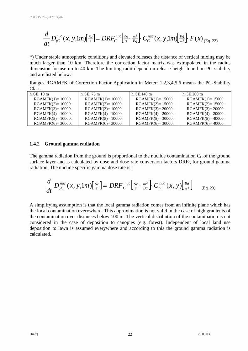
*) Under stable atmospheric conditions and elevated releases the distance of vertical mixing may be much larger than 10 km. Therefore the correction factor matrix was extrapolated in the radius dimension for use up to 40 km. The limiting radii depend on release height h and on PG-stability and are listed below:

Ranges RGAMFK of Correction Factor Application in Meter: 1,2,3,4,5,6 means the PG-Stability Class h.GE. 10 m

RGAMFK(1)= 10000. RGAMFK(2)= 10000. RGAMFK(3)= 10000. RGAMFK(4)= 10000. RGAMFK(5)= 10000. RGAMFK(6)= 30000.

h.GE. 75 m RGAMFK(1)= 10000. RGAMFK(2)= 10000. RGAMFK(3)= 10000. RGAMFK(4)= 10000. RGAMFK(5)= 10000. RGAMFK(6)= 30000.

h.GE.140 m RGAMFK(1)= 15000. RGAMFK(2)= 15000. RGAMFK(3)= 20000. RGAMFK(4)= 20000. RGAMFK(5)= 30000. RGAMFK(6)= 30000.

h.GE.200 m RGAMFK(1)= 15000. RGAMFK(2)= 15000. RGAMFK(3)= 20000. RGAMFK(4)= 20000. RGAMFK(5)= 40000. RGAMFK(6)= 40000.

1.4.2 Ground gamma radiation

The gamma radiation from the ground is proportional to the nuclide contamination CG of the ground surface layer and is calculated by dose and dose rate conversion factors DRFG for ground gamma radiation. The nuclide specific gamma dose rate is:

[ ] [ ] [ ]2

2 ),()1,,(mBqnuc

GBqm

sSvnuc

GsSvnuc

G yxCDRFmyxDdtd

⋅⋅=γ (Eq. 23)

A simplifying assumption is that the local gamma radiation comes from an infinite plane which has the local contamination everywhere. This approximation is not valid in the case of high gradients of the contamination over distances below 100 m. The vertical distribution of the contamination is not considered in the case of deposition to canopies (e.g. forest). Independent of local land use deposition to lawn is assumed everywhere and according to this the ground gamma radiation is calculated.


Draft] 20.03.03 23

2 The ATSTEP-Code

The ATSTEP code (programming language: FORTRAN) is integrated in RODOS as a subroutine of the interactive prognosis modules ALSMCprogn and QUICKPROGNO, and the automatic diagnosis-module Atstepdiagn in the subsystem ASY. ATSTEP is called in each time step of a loop of the RODOS modules corresponding to the time steps of a dispersion prognosis or diagnosis calculation. The prognosis time step length may be 10 minutes but typically is 30 or 60 minutes, the diagnosis time step length is always 10 minutes.

2.1 ATSTEP in different RODOS ASY modules

2.1.1 ATSTEP in the prognosis module ALSMCprogn

During each 30 minutes time step ATSTEP is provided with data arrays of wind, stability, dry deposition resistance, and precipitation by the Meteorological Preprocessor (MPP). The primary meteorological data that are processed for near range dispersion calculations in the MPP can come from different sources: • prognostical weather data from national numerical weather prediction,

in Germany DWD-data, in other countries ALADIN- or HIRLAM-data • user selected weather data files or weather data from hand input

2.1.2 ATSTEP in the interactive module QUICKPROGNO

If the user wants to perform quick interactive scenario calculations with artificial weather data then the system can be run without the MPP. The weather data are put in by the user directly or in the form of selected weather data files. The programme system for this purpose is QUICKPROGNO.

2.1.3 ATSTEP in the diagnosis module Atstepdiagn

During an accident of a nuclear power plant with a radioactive release to the atmosphere the Automatic Mode of the RODOS system is running. This mode allows for a real-time diagnosis of the radiological situation with a cycle time of 10 minutes. During each 10 minutes time step ATSTEP is provided with the data arrays of wind, stability, dry deposition resistances, and precipitation by the MPP, and with nuclide specific release data from the source term processed by STerm [9]. The primary meteorological data, release-, and monitoring data come from the RODOS real-time data base, where the on-line maesured data of the meteorological instrumentation and the stack instrumentation of the nuclear power plant and other measuring stations are sampled.

Direct continuation of the Diagnosis dispersion calculation in the Auto-Prognosis

There is a direct coupling of the diagnosis to the automatic prognosis calculation: the current positions, the instantaneous and time-integrated fields, and the activity contents of the puffs and all doses are transferred to the subsequent auto prognosis run. In this way the radiological situation that has developed in the past diagnosis can be smoothly continued by the prognosis.


Draft] 20.03.03 24

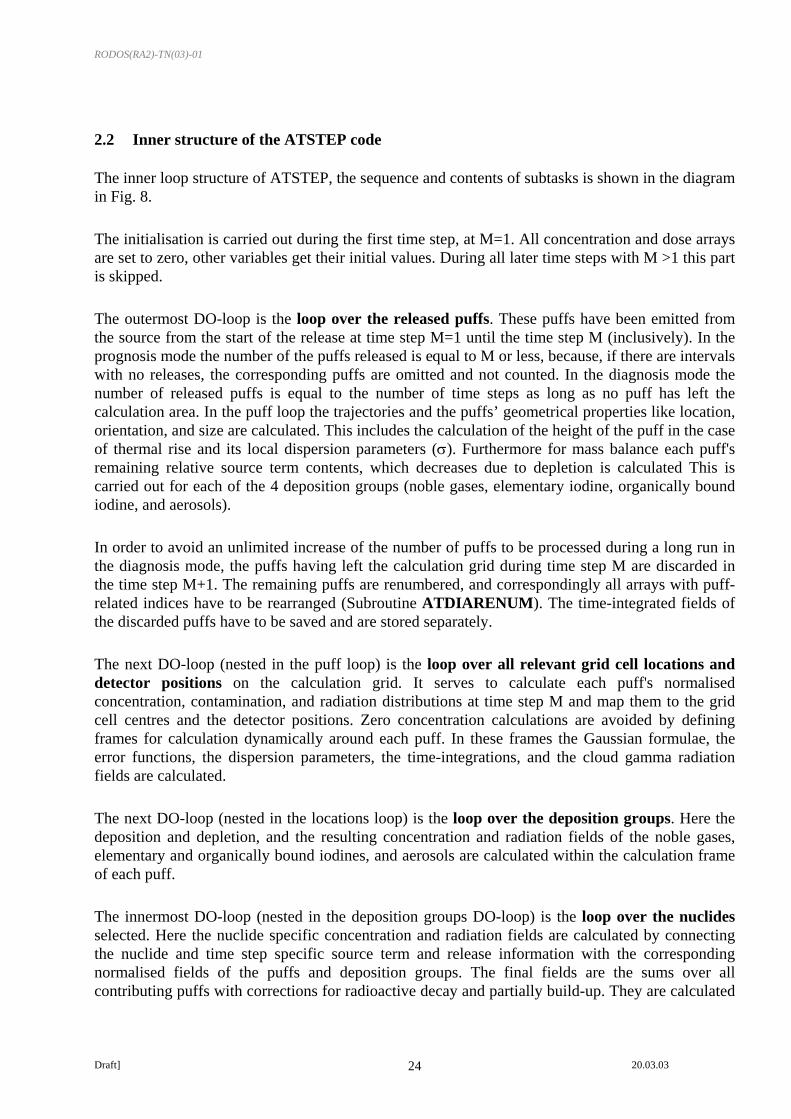
2.2 Inner structure of the ATSTEP code

The inner loop structure of ATSTEP, the sequence and contents of subtasks is shown in the diagram in Fig. 8.

The initialisation is carried out during the first time step, at M=1. All concentration and dose arrays are set to zero, other variables get their initial values. During all later time steps with M >1 this part is skipped.

The outermost DO-loop is the loop over the released puffs. These puffs have been emitted from the source from the start of the release at time step M=1 until the time step M (inclusively). In the prognosis mode the number of the puffs released is equal to M or less, because, if there are intervals with no releases, the corresponding puffs are omitted and not counted. In the diagnosis mode the number of released puffs is equal to the number of time steps as long as no puff has left the calculation area. In the puff loop the trajectories and the puffs’ geometrical properties like location, orientation, and size are calculated. This includes the calculation of the height of the puff in the case of thermal rise and its local dispersion parameters (σ). Furthermore for mass balance each puff's remaining relative source term contents, which decreases due to depletion is calculated This is carried out for each of the 4 deposition groups (noble gases, elementary iodine, organically bound iodine, and aerosols).

In order to avoid an unlimited increase of the number of puffs to be processed during a long run in the diagnosis mode, the puffs having left the calculation grid during time step M are discarded in the time step M+1. The remaining puffs are renumbered, and correspondingly all arrays with puff-related indices have to be rearranged (Subroutine ATDIARENUM). The time-integrated fields of the discarded puffs have to be saved and are stored separately.

The next DO-loop (nested in the puff loop) is the loop over all relevant grid cell locations and detector positions on the calculation grid. It serves to calculate each puff's normalised concentration, contamination, and radiation distributions at time step M and map them to the grid cell centres and the detector positions. Zero concentration calculations are avoided by defining frames for calculation dynamically around each puff. In these frames the Gaussian formulae, the error functions, the dispersion parameters, the time-integrations, and the cloud gamma radiation fields are calculated.

The next DO-loop (nested in the locations loop) is the loop over the deposition groups. Here the deposition and depletion, and the resulting concentration and radiation fields of the noble gases, elementary and organically bound iodines, and aerosols are calculated within the calculation frame of each puff.

The innermost DO-loop (nested in the deposition groups DO-loop) is the loop over the nuclides selected. Here the nuclide specific concentration and radiation fields are calculated by connecting the nuclide and time step specific source term and release information with the corresponding normalised fields of the puffs and deposition groups. The final fields are the sums over all contributing puffs with corrections for radioactive decay and partially build-up. They are calculated


Draft] 20.03.03 25

at the end of each time step and are the basic output of the RODOS near range atmospheric dispersion modules for all grid cell and detector locations, and all nuclides:

ADIFMO: concentration in air near ground, instantaneous, [Bq/m³]

ADIFSU, DET0SU: concentration in air near ground, time step averaged, [Bq/m³]

ACH1SU: time-integrated concentration in air near ground, [Bq.s/m³]

ACH2SU: contamination of lawn, dry + wet, [Bq/m2]

ACH2WU, DET2WU: contamination of lawn, wet, [Bq/m2]

ACH3MO: cloud gamma rate dispersion factor, instantaneous, [Bq/m³]

ACH3SU: cloud gamma rate dispersion factor, time step averaged, [Bq/m³]

ACH400: cloud gamma dispersion factor, time-integrated, [Bq.s/m³]

IODFRAC: iodine fractions, instantaneous

REFELD, DETRER : precipitation rate [mm/h]

After this output the DO-loops over the nuclides, the deposition groups, and the locations are finished. In the prognosis mode now those puffs are transferred to input files for the long-range dispersion module, that have left the calculation grid of the near-range module (typically at 80 km source distance). Then also the puff loop is finished.

The programme is ready for calculating the next time step in the M+1. cycle of a prognosis or diagnosis calculation. At the beginning of the M+1. time step ATSTEP needs a part of the local variables to have the values of the preceding time step M. In the prognosis mode this is done using the option „save locals on“, so the locals are saved and not set to zero automatically on subroutine call.

In the diagnosis mode this is not possible because the execution of the diagnosis module is finished after each calculation step and memory is closed down. Therefore a stop and restart mechanism is used: At the end of each diagnosis time step all geometrical information containing position and orientation of trajectories and puffs, and all time integrated fields are stored in files (Subroutine ATDIASTORE). At the beginning of each new diagnosis time step these files are read in again (Subroutine ATDIAREAD). In this way the diagnosis can be continued without forgetting the past.


Draft] 20.03.03 26

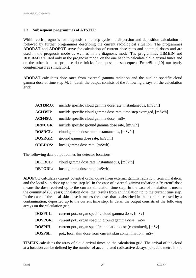
2.3 Subsequent programmes of ATSTEP

Within each prognosis- or diagnosis- time step cycle the dispersion and deposition calculation is followed by further programmes describing the current radiological situation. The programmes ADORAT and ADOPOT serve for calculation of current dose rates and potential doses and are used in the prognosis mode as well as in the diagnosis mode. The programmes TIMEIN and DOSBAU are used only in the prognosis mode, on the one hand to calculate cloud arrival times and on the other hand to produce dose bricks for a possible subsequent EmerSim [10] run (early countermeasures simulation).

ADORAT calculates dose rates from external gamma radiation and the nuclide specific cloud gamma dose at time step M. In detail the output consists of the following arrays on the calculation grid:

ACH3MO: nuclide specific cloud gamma dose rate, instantaneous, [mSv/h]

ACH3SU: nuclide specific cloud gamma dose rate, time step averaged, [mSv/h]

ACH4SU: nuclide specific cloud gamma dose, [mSv]

DRNUGR: nuclide specific ground gamma dose rate, [mSv/h]

DOSRCL: cloud gamma dose rate, instantaneous, [mSv/h]

DOSRGR: ground gamma dose rate, [mSv/h]

ODLDOS: local gamma dose rate, [mSv/h].

The following data output comes for detector locations:

DETRCL: cloud gamma dose rate, instantaneous, [mSv/h]

DETODL: local gamma dose rate, [mSv/h].

ADOPOT calculates current potential organ doses from external gamma radiation, from inhalation, and the local skin dose up to time step M. In the case of external gamma radiation a "current" dose means the dose received up to the current simulation time step. In the case of inhalation it means the committed (50 years) inhalation dose, that results from an inhalation up to the current time step. In the case of the local skin dose it means the dose, that is absorbed in the skin and caused by a contamination, deposited up to the current time step. In detail the output consists of the following arrays on the calculation grid:

DOSPCL: current pot., organ specific cloud gamma dose, [mSv]

DOSPGR: current pot., organ specific ground gamma dose, [mSv]

DOSPIH: current pot., organ specific inhalation dose (committed), [mSv]

DOSPSL: pot., local skin dose from current skin contamination, [mSv]

TIMEIN calculates the array of cloud arrival times on the calculation grid. The arrival of the cloud at a location can be defined by the number of accumulated radioactive decays per cubic metre in the


Draft] 20.03.03 27

air near ground, i.e. the time-integrated activity concentration ACH1SU summed over all nuclides [Bq.s/m3]. If this number exceeds the value 1000 [Bq.s/m3] in the M-th time step, the local arrival time of the cloud is set to the value M/2 [h]. The following array is output on the calculation grid:

TIMFEL: cloud arrival times at the locations on the calculation grid, [h]

DOSBAU: At the end of the prognosis time interval on the last day of the scenario DOSBAU generates potential dose bricks for the dose calculations with early emergency actions in EmerSim. In the case of external gamma radiation the dose brick of a specified exposure pathway and organ is defined as the amount of dose absorbed in the M-th half hour time step. In the case of inhalation or skin contamination it is defined as the amount of dose resulting from inhalation or deposition during that time step. The following arrays on the calculation grid are put out for 5 organs after each of the maximum 48 time steps of the last day of a prognosis calculation:

DBAUCL: organ specific dose brick for cloud gamma radiation, [Sv]

DBAUGR: organ specific dose brick for ground gamma radiation, [Sv], exposure time = 0.5 h

DINTGR: organ specific dose brick for ground gamma radiation, [Sv], for longer exposure with times = 1d, 7d, 14d, 30d,0.5y, 1y, 50y

DBAUIH: organ specific dose brick for inhalation, [Sv], integration times = 1d, 7d, 30d, 1y, 50y

DBAUJT: thyroid dose brick for iodine inhalation, [Sv], integration times = 50y

DBAUSL: dose brick for local skin dose by contamination, [Sv]

DBAUSLW: dose brick for local skin dose by wet contamination, [Sv]

DBAUSO: organ specific dose brick for gamma radiation from contaminated skin and clothes, [Sv]

DBAUSOW: organ specific dose brick for gamma radiation from wet contaminated skin, and clothes, [Sv]


Draft] 20.03.03 28

Loop over the puffs released during time step M

Loop over the nuclides in the deposition groups

Loop over the grid points and monitoring locations

Loop over the deposition groups

End of loops over the nuclides, deposition groups, grid points and monitors

First initializing and on each new day

Meteorological data, Transport Vectors, Geometry

Decay factors, daughter nuclides Puff trajectories

Thermal rise Travelled distance and times

Sigma-parameters Vertical wind shear- and mass profiles

depletion of puffs

local sigma-parameters, integral error functions, Gaussian formulae multiple reflections,

cloud gamma.

Transformation of puff coordinates: Translation and Rotation

Local depletion of puffs, Calculation of each puff's normalized

concentration-,contamination-, and gamma radiation fields

Connecting the puff fields to the source term: calculation of nuclide specific concentration-, contamination-, and gamma radiation fields

Transfer of leaving puffs to the Long Range Model

End of loop over the puffs

Fig. 9: Program structure of ATSTEP


Draft] 20.03.03 29

3 References [1] Panitz, H-J.,Matzerath, C., Päsler-Sauer, J.,UFOMOD, Atmospheric Dispersion and

Deposition, Report KfK-4332, (1989) [2] Störfall-Leitlinien, Bundesanzeiger, Jahrg. 35, Nummer 245a, 1983, Der Bundesminister der

Justiz. [3] German French Commission, Das deutsch-französische Modell für die atmosphärische

Ausbreitung in Unfallsituationen, DFK-Bericht 92/2, AG3, 06.1992, Dresden. [4] Hanna, S. R., Briggs, G. A., Hosker, R. P., Handbook on Atmospheric Dispersion, U. S.

Department of Energy, 1982, DOE/TIC-11223, S. 31 [5] Briggs, G. A., Plume Rise Predictions, in Lectures on Air Pollution and Environmental

Impact Analyses, Workshop Proceedings, Boston, Mass., 1975, AMS, Boston, Mass. [6] Müller, H., Gering, F.,Documentation of the Deposition Module in RODOS PV5.0, Technical

Note RODOS(RA3)-TN(02)01. [7] Schwarz, G.,Deposition and Post-Deposition Radionuclide Behaviour in Urban

Environments, Proceed. of Workshop on Methods for Assessing the off-site Radiological Consequences of Nuclear Accidents, 15-19 April 1985, Luxembourg, Commission of the European Communities, Report EUR 10397 EN, 1986, p. 542

[8] Jacob, P., Müller,H.M., Gamma Exposure from Bi-Gaussian Clouds, GSF. [9] Landman, C., Code Package STerm in RODOS PV 5.0, RODOS technical note,

RODOS(RA1) TN(02)-01 [10] Päsler-Sauer, J., Model Description of the Early Countermeasures Module EmerSim in

RODOS PV 6.0, RODOS technical note, RODOS(RA3) TN(04)-03 [11] Deaves, D.M., Hebden, C.R., Aspects of Dispersion following an Explosive Release, Atkins

Process, Document of the UK Atmospheric Dispersion Modelling Liasion Comittee


Draft] 20.03.03 30

Document History Document Title: Description of the Atmospheric Dispersion Model ATSTEP Version RODOS PV 6.0 Final RODOS number: RODOS(RA2)-TN(04)-03) Version and status: Version 2.0 (draft) Authors/Editors: Jürgen Päsler-Sauer

Address: Forschungszentrum Karlsruhe GmbH

Institut für Kern- und Energietechnik Postfach 3640 D-76021 Karlsruhe Issued by: FZK RODOS Team History: none Date of Issue: June 2004 Circulation: all File Name: ATSTEP2007.doc Date of print: July 30, 2007

RODOS migration - resy5.iket.kit.edu€¦ · considered in the modelling of atmospheric dispersion...

Documents

Transcript of RODOS migration - resy5.iket.kit.edu€¦ · considered in the modelling of atmospheric dispersion...