Rodica Curtu and Bard Ermentrout- Oscillations in a refractory neural net

$: Rodica Curtu and Bard Ermentrout- Oscillations in a refractory neural net$
8/3/2019 Rodica Curtu and Bard Ermentrout- Oscillations in a refractory neural net

http://slidepdf.com/reader/full/rodica-curtu-and-bard-ermentrout-oscillations-in-a-refractory-neural-net 1/20

Digital Object Identifier (DOI):10.1007/s002850100089

J. Math. Biol. 43, 81–100 (2001) Mathematical Biology

Rodica Curtu · Bard Ermentrout

Oscillations in a refractory neural net

Received: 14 February 2000 / Revised version: 1 August 2000 / Published online: 18 June 2001 – c Springer-Verlag 2001

Abstract. A functional differential equation that arises from the classic theory of neuralnetworks is considered. As the length of the absolute refractory period is varied, there is,as shown here, a super-critical Hopf bifurcation. As the ratio of the refractory period to thetime constant of the network increases, a novel relaxation oscillation occurs. Some approx-

imations are made and the period of this oscillation is computed.

1. Introduction

Wilson and Cowan [10] introduced a class of neural network equations modeling

the excitatory and inhibitory interactions between two populations of cells. Each

population obeys a functional-differential equation of the form:

τ du(t)

dt = −u(t) + (1 − t

t −Ru(s) ds)f (I (t))

where τ is the time constant, I(t) represents inputs to the population, f is the firing

rate curve, and R is the absolute refractory period of the neurons. The function u(t)

is the fraction of the population of neurons which is firing. It can also be regarded

as the actual firing rate of the population. The refractory term premultiplying the

firing rate was approximated (by assuming that R is small) as

1 − t

t −R

u(s) ds ≈ 1 − Ru(t).

All subsequent analyses of these equations either make this assumption or set

R = 0.

There have been numerous analyses of neural networks with delays. Castel-

franco and Stech [2] prove the existence of oscillatory solutions to a two-

dimensional model due to Plant which has delayed negative feedback. Similar

results are described by Campbell et al. in a model for pupillary control [1].

Marcus and Westervelt [9] linearize a Hopfield symmetrically coupled network

This work was supported in part by the National Science Foundation and NIMH.

R. Curtu, B. Ermentrout (for correspondence): Department of Mathematics, University of Pittsburgh, Pittsburgh PA 15260, USA. e-mail: [email protected]

Key words or phrases: Delay equations – Hopf bifurcation – Neural networks – Relaxationoscillation



82 R. Curtu, B. Ermentrout

and show that the fixed points are asymptotically stable. Ye et al. [11] improve on

this result by rigorously showing global stability of fixed points for the Hopfield

network with delay.

The purpose of this note is to explore the consequences of keeping the originalform of the Wilson-Cowan equations. In particular, we will look at a self-excited

population of cells. We consider the functional-differential equation

τ du

dt = −u +

1 −

1

R

t

t −R

u(s) ds

f (u)

where f is a smooth monotonically increasing function ( f > 0 ) which takes

values between 0 and 1. We have normalized the integral term in order to study the

temporal effects of altering this absolute refractory period.By rescaling the time t → t /R and letting r = R/τ denote the ratio of the

absolute refractory period to the time constant of the network, the equation becomes

du

dt = r

−u +

1 −

t

t −1

u(s)ds

f(u)

(1)

We can alternatively rescale time as t → t /τ and obtain:

du

dt = −u +

1 − 1

r

t

t −r

u(s)ds

f (u).

In this rescaling, it is clear that this is a “delayed negative-feedback” system and

that in the limit as r → 0 we obtain the original Wilson-Cowan equations

du

dt = −u + (1 − u)f (u).

Because the calculations are simpler, we will use the first rescaling, (1) in theremainder of the paper.

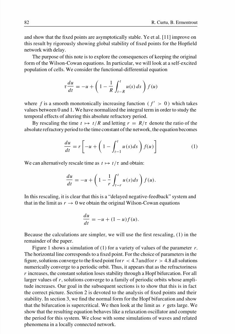
Figure 1 shows a simulation of (1) for a variety of values of the parameter r.

The horizontal line corresponds to a fixed point. For the choice of parameters in the

figure, solutions converge to the fixed point for r < 4.7andfor r > 4.8 all solutions

numerically converge to a periodic orbit. Thus, it appears that as the refractoriness

r increases, the constant solution loses stability through a Hopf bifurcation. For all

larger values of r , solutions converge to a family of periodic orbits whose ampli-

tude increases. Our goal in the subsequent sections is to show that this is in fact

the correct picture. Section 2 is devoted to the analysis of fixed points and theirstability. In section 3, we find the normal form for the Hopf bifurcation and show

that the bifurcation is supercritical. We then look at the limit as r gets large. We

show that the resulting equation behaves like a relaxation oscillator and compute

the period for this system. We close with some simulations of waves and related

phenomena in a locally connected network.



Oscillations in a refractory neural net 83

0

0.2

0.4

0.6

0.8

1

u(t)

200 201 202 203 204 205 206 207 208t

r=4.9r=8

r=100

Fig. 1. The behavior of (1) for different values of the parameter r = R/τ with f(u) =1/(1 + exp(−8(u − .333))). The period of the smallest oscillation is 4 and that of the largestis 1.43.

2. Fixed points and stability

The fixed points for (1) are u = u for all t and u satisfies

−u + (1 − u)f(u) = 0 (2)

It is easy to check that because 0 < f < 1 there is no equilibrium point in (−∞, 0] ∪

[ 12

, ∞), but there is at least one in (0, 12

), say u.

For such an equilibrium we can rewrite the equation (1), by defining u := u + y

and using the Taylor expansion for the function f about u, as

dy

dt = r

−y + y (1 − u) f

(u) − f (u) t

t −1 y(s)ds

+ r

−y f (u)

t

t −1

y(s)ds + y2(1 − u)f (u)

2

+ r

−y2 f (u)

2

t

t −1

y(s)ds + y3 (1 − u)f (u)

6

+ O(y4) (3)




As a first step in our analysis we will consider only the linearized part of the equation

(3), i.e.

dy

dt = r

−A y − b t

t −1 y(s)ds

where the coefficients A and b are given by A = 1 − (1 − u) f (u) < 1 and

b = f (u) ∈ (0, 1).

The stability of this equation is determined by studying the roots of the charac-

teristic equation obtained by substituting y(t) = exp λt into the linearized equation.

This results in

λ + A r + b r1 − e−λ

λ. (4)

A very similar equation to this is studied in Diekmann et al., Chapter XI.4.3. We

summarize the main points as they apply to the present equations. First, λ = 0 if

and only if A + b = 0 and furthermore as long as b = 0, λ = 0 is a simple root.

All roots with positive real part are bounded by the following inequality:

|λ| < r(|A| + |b|).

Thus, the only way that roots can enter the right-half plane is to go through the

imaginary axis. Clearly if b = 0 and A > 0, then all roots have negative real parts.

Furthermore, as we just noted, roots can cross 0 only if A + b = 0. Thus, we areinterested in when there are roots of the form λ = iω . Substituting this into (4) we

see that

Ar = −ω sin ω

1 − cos ω, (5)

br =ω2

1 − cos ω. (6)

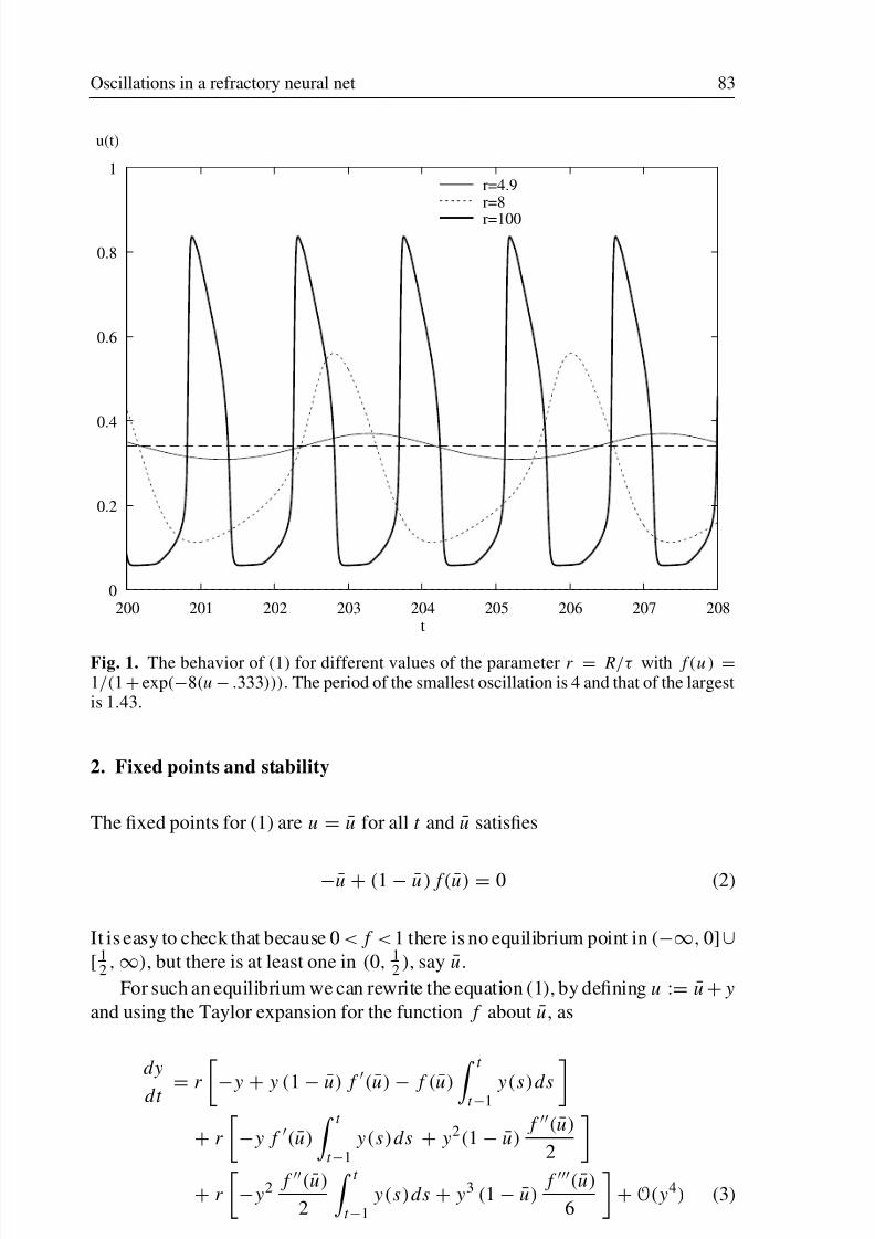
Since there are singularities at ω = 2kπ , these equations define a series of para-

metric curves defined in the regions ω ∈ (2kπ, 2(k + 1)π) for k an integer. Thefirst two of these curves are plotted in Figure 2. Crossing these curves results in

new complex eigenvalues with positive real parts. To study stability as a function of

the parameter r , we note that (Ar, br) defines a line through the origin with slope

b/A as r varies in the the (Ar, br) plane shown in the figure. If this line crosses the

lower emphasized curve then stability is lost through a pair of complex eigenvalues

as the parameter r increases. Taking the ratio of the two above equations, we see

that there will be such a root if and only if:

A

b = −sin ω

ω . (7)

The minimum of this function is −1 and the maximum is M = − sin(ξ)/ξ where

ξ is the smallest root of tan(x) = x greater than π. Thus, the slope of the line

b/A must lie between 1/M ≈ 4.60334 and −1. These two lines are illustrated in

Figure 2. If b/A lies between −1 and 4.6033 . . . , then starting at small values of r




Fig. 2. Stability diagram for (4) as a function of A r and b r . Straight lines depicts the curveb = −A and b = A/M where M is defined in the text. The remaining curves depict linesalong which there are purely imaginary roots. Numbers denote the number of eigenvalueswith positive real parts.

as r increases, it pierces the lower stability curve and a pair of complex conjugate

eigenvalues cross the imaginary axis resulting in a loss of stability. Clearly, if b/A

is within these bounds, then we can solve (7) for a value of ω between 0 and 2π.

Then we can use (6) to find

r0 =1

b

ω2

1 − cos ω

the critical value of r (which is always positive). If b/A is positive and less than

1/M then no increases in r can ever lead to a loss of stability. If the slope b/A

is negative and shallower than −1, then for all positive values of r there is a real

positive root to (4). To see this, note that we can rewrite (4) as

br1 − e−λ

λ

= −(λ + Ar).

The left-hand side is monotonically decreasing, positive, and starts at br at λ = 0.

Suppose that −Ar > br. Then −(λ + Ar) is larger than br at λ = 0 and crosses the

x-axis when λ = −Ar > 0. Thus, there is an intersection of the two for a positive

value of λ between 0 and −Ar.

We summarize these calculations in the following theorem.




Theorem 1. Suppose u is a fixed point of the equation (1). Let A = 1−(1−u) f (u)

and b = f (u).

• Suppose that −b < A < b M where M = − sin(ξ)/ξ ≈ 1/4.60334 =

0.2172336 with ξ the smallest root greater than π to tan(x) = x. Then for

r small enough, the fixed point is stable. As r increases, stability is lost when r

crosses r0 where

r0 =1

b

ω20

1 − cos ω0

and ω0 is the unique root to

A

b= −

sin ω

ω

between 0 and 2π.

• If A > Mb then the fixed point is stable for all values of r.

• If A < −b then the fixed point is unstable for all positive r .

3. Normal form

The numerical simulations in figure 1 indicate that there exist oscillatory solutionsfor large enough r . Because of the above stability analysis we suspect the presence

of an Andronov-Hopf bifurcation point for certain values of the parameter r . The

next reasonable step would be the construction of the corresponding normal form

and this is exactly what we do in this section. The Hopf bifurcation theorem has

been rigorously proven for (1) and related equations in Diekmann, et.al.[3] Indeed,

the authors compute the normal form for a related equation in Chapter XI4.3. Faria

and Magalhaes [4] describe a method to compute normal forms using the adjoint

for equations of the form:

dz

dt = L(p)zt + F (zt , p)

where p represents parameters. Our approach is similar to theirs. With minor

modifications, we could apply the formula in Theorem 3.9 Diekmann, et al. [3]

(page 298), but for completeness, we derive the coefficients for the normal form

here.

Let us consider the equation (3) and define the linear operators

Ly :=dy

dt + A r0 y + b r0

t

t −1

y(s)ds

y := −A y − b

t

t −1

y(s)ds




as well as the quadratic and cubic forms

B(y1, y2) := r0 (1 − u)f (u)

2

y1 y2 −f (u)

2

y1 t

t −1

y2(s)ds

−f (u)

2y2

t

t −1

y1(s)ds

C(y1, y2, y3) := r0

(1 − u)f (u)

6y1 y2 y3 −

f (u)

6y1 y2

t

t −1

y3(s)ds

−f (u)

6y2 y3

t

t −1

y1(s)ds −f (u)

6y3 y1

t

t −1

y2(s)ds

Taking a small perturbation of the parameter (r = r0 + α), the equation (3) can be

rewritten as

Ly = αy + B(y,y) + C(y,y,y) + αB(y,y) + O(y4) (8)

Since we are interested in finding small oscillatory solutions we can consider the

following asymptotic expansion for (small) y and α

α = α1 + 2α2 + 3α3 + · · ·

y(t) = u0(t) + 2u1(t) + 3u2(t) + · · · → 0

and obtain, instead of (8),

Lu0 + 2Lu1 + 3Lu2 +O(4)

= [ α1 + 2α2 + 3α3 + · · · ] · [ u0 + 2u1 + 3u2 + · · · ]

+ [1 + α1 + · · · ] · B( u0 + 2u1 + 3u2 + · · · , u0 + 2u1 + 3u2 + · · · )

+ C( u0 + 2u1 + 3u2 + · · · , u0 + 2u1 + 3u2 + · · · , u0 + 2u1

+ 3u2 + · · · ) + O(4) as → 0

or, equivalently,

Lu0 + 2Lu1 + 3Lu2 +O(4)

= 2 [ α1 u0 + B(u0, u0) ] + 3 [ α1 u1 + α2 u0 + 2B(u0, u1)

+ C(u0, u0, u0) + α1 B(u0, u0)] +O(4). (9)

Based on the fact that the equation Ly = 0 has two independent solutions (e± iω0t )

on the center manifold and by the asymptotic expansion

Lu0 = [α1 u0 + B(u0, u0) − Lu1] + · · ·

we can choose

u0(t) = z(t)eiω0t + z(t)e−iω0t




with z depending on (e.g. z = z(2t)). The expansion with respect to gives

z = z(0) + 2t z(0) + O(4) as tends to 0. We then use z and the properties of

the defined operators and obtain

0 = [ α1 z(0) (eiω0t ) + α1 z(0)(e−iω0t ) + 2z(0)z(0)B(eiω0t , e−iω0t )

+z(0)2B(eiω0t , eiω0t ) + z(0)2B(e−iω0t , e−iω0t ) − Lu1 ]

+2[ −Lu2 − z(0)L(teiω0t ) − z(0)L(te−iω0t ) + α1 u1

+α2 z(0)(eiω0t ) + α2 z(0)(e−iω0t ) + 2B(u0, u1) + α1 B(u0, u0)

+C(u0, u0, u0) ] +O(3). (10)

The coefficient of should be zero on the center manifold. This implies that at

= 0 we must solve Lu1 = g, with the given function g,

g(t) = α1 z(0)(eiω0t ) + α1 z(0)(e−iω0t ) + 2z(0)z(0)B(eiω0t , e−iω0t )

+ z(0)2B(eiω0t , eiω0t ) + z(0)2B(e−iω0t , e−iω0t ).

In order to ensure the existence of a solution for the equation Lu1 = g we

need the inhomogeneous term g(t) to be orthogonal to the solutions of the adjoint

homogeneous equation. The adjoint operator of L (see appendix A) is L∗y :=

−dydt

+ A r0 y + b r0

t +1

t y(s)ds, and on the two-dimensional center manifold

eiω0t and e−iω0t are independent solutions for L∗. The inner product is the usual

one: < φ , ψ >= 2πω0

0 φ(t)ψ(t)dt , so we need

2πω0

0

g(t)e± iω0t dt = 0.

Using the identities which are proven in appendix B,

L(eλt ) = L(λ) eλt

(e

λt

) =˜

(λ) e

λt

B(eλ1t , eλ2t ) = B(λ1, λ2) e(λ1+λ2)t

C(eλ1t , eλ2t , eλ3t ) = C(λ1, λ2, λ3) e(λ1+λ2+λ3)t

for certain functions L, , B and C, the function g can be expressed as a linear

combination of powers of eiω0t and e−iω0t . The orthogonality condition becomesα1 z(0) 2π

ω0(−iω0) = 0

α1 z(0) 2πω0

(iω0) = 0

Obviously in this case α1 is zero, and the equation corresponding to u1 is on the

center manifold

Lu1 = z(0)2 B(iω0, iω0) e2iω0t + z(0)2 B(−iω0, −iω0) e−2iω0t

+2z(0)z(0) B(iω0, −iω0) (11)




Choose

u1 = a1z2e2iω0t + 2a2zz + a3z2e−2iω0t

⇓

u1 = a1z2(0)e2iω0t + 2a2z(0)z(0) + a3z2(0)e−2iω0t +O(2t) as → 0

and introduce in L and compare with (11). We get the coefficients a1, a2, a3,

a1 =B(iω0, iω0)

L(2iω0)

a2 =B(iω0, −iω0)

L(0)

a3 =

B(−iω0, −iω0)

L(−2iω0)

with a2 ∈ R and a1 = a3.

So far we have calculated u0, u1, α1. We can now conclude that in the equation

(10), u2 should satisfy

Lu2 = − z(0)L(teiω0t ) − z(0)L(te−iω0t )

+ α2 z(0) (iω0)eiω0t + α2 z(0)(−iω0)e−iω0t

+ 2a1 z3(0)B(eiω0t , e2iω0t ) + 4a2 z2(0)z(0)B(eiω0t , 1)

+ 2a3 z3(0)B(e−iω0t , e−2iω0t ) + 4a2 z(0)z2(0)B(e−iω0t , 1)

+ 2a1 z2(0)z(0)B(e−iω0t , e2iω0t ) + 2a3 z(0)z2(0)B(eiω0t , e−2iω0t )

+ z3(0)C(eiω0t , eiω0t , eiω0t ) + 3z2(0)z(0)C(eiω0t , eiω0t , e−iω0t )

+ z3(0)C(e−iω0t , e−iω0t , e−iω0t ) + 3z(0)z2(0)C(eiω0t , e−iω0t , e−iω0t )

Similar to what we have already seen for u1, in order to have solutions, we need

the right hand side to be orthogonal on e± iω0t , i.e

z(0)

2πω0

0

e−iω0t L(teiω0t ) dt + z(0)

2πω0

0

e−iω0t L(te−iω0t ) dt

= α2 z(0) (iω0)2π

ω0

+ 2a1 z2(0)z(0) B(−iω0, 2iω0)2π

ω0

+ 4a2 z2(0)z(0) B(iω0, 0)2π

ω0+ 3z2(0)z(0) C(iω0, iω0, −iω0)

2π

ω0

and, finally,

z(0) =i ω0 α2

r0 2 + A r0 + i(ω0 − A r0+b r0

ω0

)z(0)

+4a2 B(iω0, 0) + 2a1 B(−iω0, 2iω0) + 3C(iω0, iω0, −iω0)

2 + A r0 + i(ω0 − A r0+b r0

ω0)

z2(0)z(0)

(12)

with specific values for B and C calculated in Appendix B.




We have just proven the following theorem.

Theorem 2. Suppose that u is an equilibrium point of the equation (1) and that

A, b satisfy −b < A < M b where M is as in Theorem 1. Take r0 and ω0 as in

Theorem 1 and denote by δ the coefficient of z2(0)z(0) in (12).Then the normal form on the center manifold at r = r0 is given by (12). If

Re(δ) < 0 (Re(δ) > 0) then at r = r0 the system passes through a supercritical

(subcritical) Andronov-Hopf bifurcation which proves the existence of a small am-

plitude periodic stable (unstable) solution in the vicinity of the steady state near

the bifurcation point.

Proof. The nondegeneracy condition requires the real part of the coefficient of z(0)

to be nonzero. The real part of the coefficient is

ω20 − (A + b)r0

r0[(2 + Ar0)2 + (ω0 − (A + b)r0/ω0)2].

Substitution of r0 = ω20/[b(1 − cos ω0)] into the numerator and using the fact that

A/b = − sin(ω0)/ω0 we find that the numerator is

ω20

1 − cos ω0

sin ω0

ω0− cos ω0

.

The first term cannot vanish since ω0

∈ (0, 2π ). Thus, the coefficient will be zero

if and only if

sin ω0

ω0

= cos ω0.

Recall that the extrema of sin(ω)/ω = −A/b can occur only when sin(ω)/ω =

cos ω so that the numerator will vanish only along the lines A = −b and A = Mb.

Since −b < A < bM this is impossible.

3.1. Example

We consider the function

f(x) =1

1 + e−a(x +θ )with a = 8, θ = −0.333.

There is only one equilibrium point u . We compute A, b and the values for the first

three derivatives

u = 0.335909

A = −0.328002b = 0.505818

f (u) = 1.99973

f (u) = −0.186145

f (u) = −63.9653




and solve for ω and r . There is a unique solution

ω0 = 1.541455 and

r0

= 4.839469881

By immediate calculation sin(ω0)/ω0 − cos ω0 = 0.619121, so the linear coeffi-

cient in the normal form is positive and the rest state loses stability when the value

of r increases through r = r0. At r = r0 a stable periodic orbit is born. In this

example the quantities which appear in the formula for the coefficient of z2z in the

normal form are

2 + Ar0 + i(ω0 −r0(A + b)

ω0) = 0.4126442001 + 0.9831933729 i

L(0) = 0.8605351764L(2iω0) = −1.54079164 + 1.496237313 i

B(iω0, 0) = −8.275709357 + 3.047038468 i

B(−iω0, 2iω0) = −3.52893752 + 0.0893831027 i

B(iω0, −iω0) = −6.574664704

B(iω0, iω0) = −6.574664704 + 6.094076935 i

C(iω0, iω0, −iω0) = −33.97038306 − 0.0945445928 i

a1 = 4.172849433 + 0.097025506 i

a2 = −7.640204473

δ = −36.6125 − 138.977 i

Obviously since Re(δ) < 0 this is a supercritical Andronov-Hopf bifurcation.

We note that Figure 1 shows the numerical solutions for a variety of values of

r. In particular, the fixed point is the only attractor for r = 4.7 but clearly, when

r = 4.9 there is a stable periodic solution. The period computed analytically is

2π/ω0 = 4.08 which agrees well with the numerically found period of 4.00. Thus,

the numerical solutions and the Hopf calculations are consistent.

4. Relaxation oscillator

We now consider equation (1) for large values of the parameter r . By introducing

= 1r

and the function z(t)

z(t) :=

t

t −1

u(s) ds

equation (1) is equivalent to the two-dimensional delay-differential equationdu/dt = −u + (1 − z)f(u)

dz/dt = u(t) − u(t − 1)(13)

We recall that (1) is obtained by rescaling time t with respect to the parameter r

in the original equation, so t represents a slow time. We analyze the solution by




treating as a small positive parameter. We will first point out how to construct

a singular periodic orbit for this system and then we will estimate the period T

for the relaxation oscillator. Mallet-Paret and Nussbaum [8] have extensively and

rigorously analyzed an equation similar to (13):

dx(t)

dt = −x(t) + f(x(t − 1))

where f is an odd negative feedback function (that is, xf (x) ≤ 0). In particular,

they consider a step function for f. Hale and Huang [5] have studied the vector

analogue:

dx(t)

dt = −Ax(t) + Af (λ, x(t − 1))

where A is an invertible matrix and f is smoothly dependent on x and the free pa-

rameter λ. They assume that the map x −→ f(λ,x) undergoes a period-doubling

bifurcation at λ = 0 and then prove that the delay-differential equation undergoes

a similar bifurcation. More recent work by Hale and Huang [6] shows a similar

behavior as well as a Hopf bifurcation. As far as we know, however, the rigorous

analysis of equation (13) has not been done and remains an open problem. Our

approach is formal and approximate.

By setting = 0 in (13), we obtain the equations corresponding to the slow

flow 0 = −u + (1 − z)f(u)

dz/dt = u(t) − u(t − 1)(14)

For the fast flow we consider the original integro-differential equation. In this case

the function z is z(t) = 1r

t t −r

u(s)ds and it satisfies

dz/dt = (u(t) − u(t − r))/r.

When r tends to infinity ( tends to zero), the system becomesdu/dt = −u + (1 − z)f(u)

dz/dt = 0

Thus, the two-dimensional system is decomposed in two one-dimensional equa-

tions, the solutions of which we now characterize.

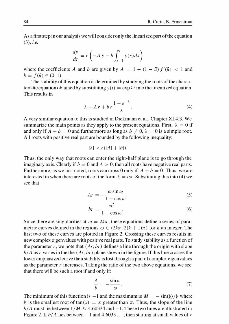
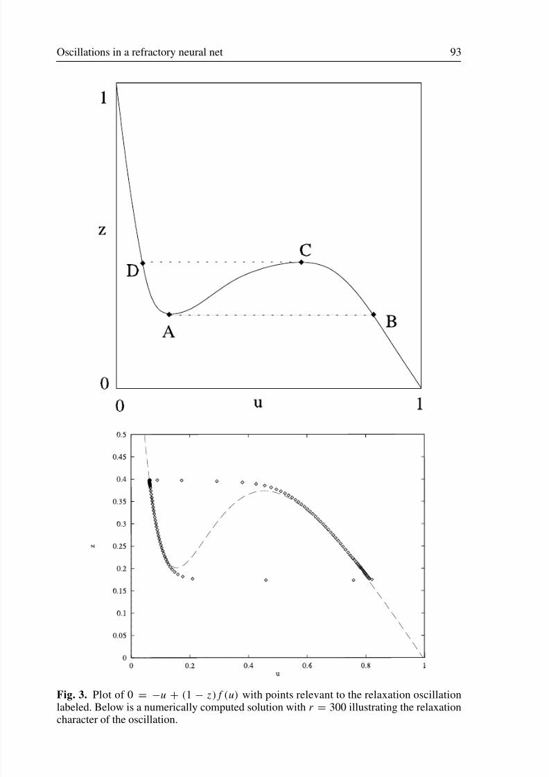
Consider the graph for

0 = −u + (1 − z)f(u)

with f(x) =1

1 + e−a ( x+θ ), a = 8, θ = −0.333

The sign of (−u + (1 − z)f(u)) is negative above the graph and positive below

it. Consider the points A , B , C , D on the graph with corresponding coordinates:

A(u1, zmin) , B(umax, zmin) , C(u2, zmax) , D(umin, zmax). (See Figure 3.) We




Fig. 3. Plot of 0 = −u + (1 − z)f (u) with points relevant to the relaxation oscillationlabeled. Below is a numerically computed solution with r = 300 illustrating the relaxationcharacter of the oscillation.




begin with the system at the point A at t = 0, where z cannot decreases anymore

so a jump up takes place to the BC branch ( z = constant and u suddenly increas-

es by the fast system). On this branch the system’s law of motion is (14). Here

dz/dt > 0 so z increases until the point reaches C. We remark that in order tohave dz/dt > 0 on BC branch we need u(t) > u(t − 1) all the time. This is

obviously true at B since uB = u(t = 0+) = umax > u(t = −1). In order to

have uC = u(t = T d ) > u(t = T d − 1) we need u(t = T d − 1) to be on the DA

branch. This implies that T d must be less than 1.

At the point C since z cannot increases anymore there is a jump down to the

branch DA ( z = constant and u decreases by the fast system). On the branch DA,z

decreases from zmax to zmin. In order to have dz/dt < 0 we need u(t) < u(t − 1),

in particular uD = u(t = T d +) = umin < u(t = T d − 1) and uA = u(t = T ) <

u(t = T − 1), which means that it is necessary that u(T − 1) be on the BC branch,

i.e. T − 1 is positive and less than T d .

Following these considerations we see that in order to construct a singular

periodic solution it has to be true that

0 < T − 1 < T d < 1 < T (⇒ T < 2)

where T is the period of oscillation and T d is the time the system stays on the upper

branch BC. We estimate T and T d considering u constant: (u = uH ) on the branch

BC and u = uL on the branch DA.

At t = 0, z = zmin

, u = uH and

dz/dt = u(t) − u(t − 1) =

0 , t ∈ [0, T d + 1 − T ]

uH − uL , t ∈ [T d + 1 − T , T d ]

0 , t ∈ [T d , 1]

uL − uH , t ∈ [1, T ]

equivalently with

z(t) =

zmin , t ∈ [0, T d + 1 − T ]

(uH − uL) t + C1 , t ∈ [T d + 1 − T , T d ]

C2 , t ∈ [T d , 1]

(uL − uH ) t , t ∈ [1, T ]

with z(T ) = zmin and z(T d ) = zmax. Using this and the identity z(t = 0) =

zmin = 0

−1 u(s)ds we obtain an estimate for T and T d

T = 1 + zmax−zmin

uH −uLand

T d = zmax−uL

uH −uL

For our example

umin = 0.065 u1 = 0.15957447

umax = 0.777 u2 = 0.45106383

zmin = 0.20141882 zmax = 0.37353106




Choosing uH = umin and uL = umin we have

T = 1.2417 T d = 0.4333

The period for the oscillation shown in Figure 3 is 1.35. Given that u is not reallyconstant on the branches, this is a pretty good estimate of the period. We can im-

prove this estimate with just a minor change in the choice of uL and uH . Above,

we chose umax and umin. A better estimate is to choose the mean value:

uL =umin + u1

2, uH =

u2 + umax

2.

For our example, this implies uL = 0.1122872, uH = 0.6140319 and

T = 1.3430, T d = 0.5206.

This is a considerably better estimate of the period without any extra work.

5. Discussion and further developments

We have analyzed the original Wilson-Cowan model for an excitatory population of

neurons with an absolute refractory period. It is not surprising that there exist oscil-

lations as the system is essentially a delayed negative feedback model. Curiously,

however, as the effective delay increases, the oscillation converges to a relaxation-

like pattern and the frequency goes to a nice limit. In terms of the original time, theactual oscillation period scales linearly with R the absolute refractory period.

We have looked only at oscillatory solutions of the scalar problem. What hap-

pens when twopopulations are coupled? Will the resulting oscillations synchronize?

For example, what is the nature of solutions to

duj

dt = r

1 −

t

t −1

u(s) ds

f (uj + gu3−j ) j = 1, 2,

where g is the coupling coefficient? Numerical solutions of this indicate that all

initial conditions tend to the synchronous state. We can use the results of section3 to understand why this is true, at least near the Hopf bifurcation. Letting g be a

small parameter, the normal form for the weakly coupled system is

zj = zj N (|zj |) + dz3−j j = 1, 2.

N(v) = c(r − r0) + δv2 where δ was calculated in section 4. The coefficient

d = (1 − u)f (u) is real and positive. Thus, the synchronous solution is always a

stable solution. (These results follow from Hoppensteadt and Izhikevich, [7]).

If we let a be larger in the definition of the function f , then the system is not

oscillatory but rather excitable. That is, a small initial condition decays back to 0but a large value grows rapidly before decaying to rest. This suggests that a line of

such units coupled locally can generate a traveling wave. Consider

uj = −uj +

1 −

t

t −1

uj (s) ds

f (

1

3

k

uk )




0.1

0.2

0.3

0.4

0.5

0.6

0.7

u(j,t)

0 1 2 3 4 5t

4 8 12 16

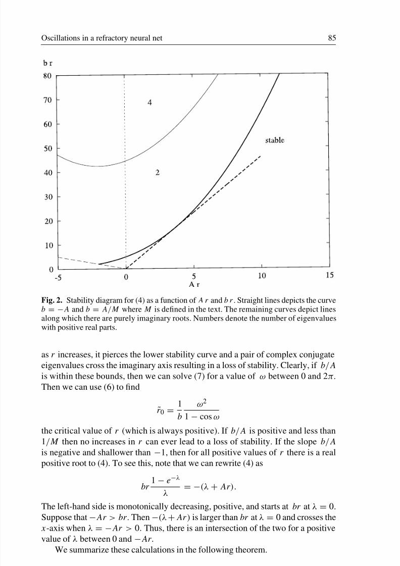
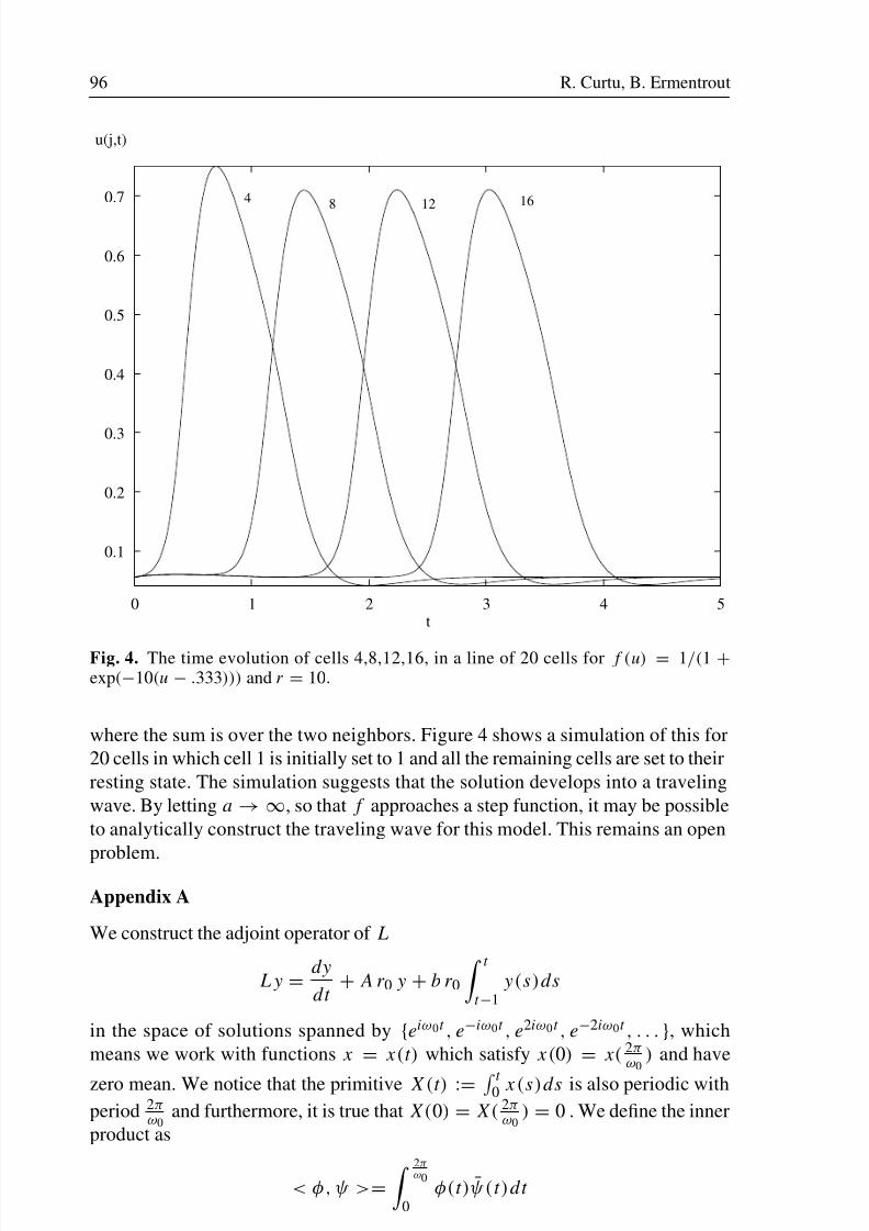
Fig. 4. The time evolution of cells 4,8,12,16, in a line of 20 cells for f (u) = 1/(1 +exp(−10(u − .333))) and r = 10.

where the sum is over the two neighbors. Figure 4 shows a simulation of this for

20 cells in which cell 1 is initially set to 1 and all the remaining cells are set to their

resting state. The simulation suggests that the solution develops into a traveling

wave. By letting a → ∞, so that f approaches a step function, it may be possible

to analytically construct the traveling wave for this model. This remains an open

problem.

Appendix A

We construct the adjoint operator of L

Ly =dy

dt + A r0 y + b r0

t

t −1

y(s)ds

in the space of solutions spanned by {eiω0t , e−iω0t , e2iω0t , e−2iω0t , . . . }, which

means we work with functions x = x(t) which satisfy x(0) = x( 2πω0

) and have

zero mean. We notice that the primitive X(t) :=

t 0 x(s)ds is also periodic with

period 2πω0

and furthermore, it is true that X(0) = X( 2πω0

) = 0 . We define the inner

product as

< φ , ψ >=

2πω0

0

φ(t)ψ(t)dt




Now for any two functions x, y in this space < x, Ly >=< L∗x , y > , where L∗

is the adjoint of the operator L.

Compute < x, Ly > :

< x, Ly > =

2πω0

0

x(t)

dy

dt + A r0 y + b r0

t

t −1

y(s)ds

= x(t) y(t)|2πω0

0 −

2πω0

0

dx

dt y(t)dt + A r0

2πω0

0

x(t) y(t)dt

+ b r0

2πω0

0

x(t)

t

t −1

y(s)ds

= − 2π

ω0

0dxdt

y(t)dt + A r0 2π

ω0

0x(t) y(t)dt

+ b r0

2πω0

0

x(t)

t

0

y(s)ds − x(t)

t −1

0

y(s)ds

=

2πω0

0

A r0 x(t) −

dx

dt

y(t)dt

+ b r0 2πω0

0

x(t) Y ( t ) d t − 2πω0

0

x(t) Y (t − 1) dt Since x = dX

dt and y = dY

dt we use integration by parts and the properties of the

functions X and Y to get

< x, Ly > =

2πω0

0

A r0 x(t) −

dx

dt

y(t)dt − b r0

2πω0

0

t

0

x(s)ds

y(t)dt

+ b r0 2πω0

−1

−1

X(t + 1) y(t)dt

=

2πω0

0

A r0 x(t)−

dx

dt −b r0

t

0

x(s)ds + b r0

t +1

0

x(s)ds

y(t)dt

+ b r0

0

−1

X(t + 1)y(t)dt − b r0

2πω0

2πω0

−1

X(t + 1)y(t)dt

After a change of dummy variables in the last integral we get

< x, Ly >= 2π

ω0

0

A r0 x(t) −

dx

dt + b r0 t +1

t x(s)ds

y(t)dt

The adjoint operator is

L∗x = −dx

dt + A r0 x + b r0

t +1

t

x(s)ds




By direct calculation we see that L∗(e± iω0t ) = 0. We use for this both λ0 =

± iω0 and the characteristic equation (4).

Appendix B

Directly from the definition of the operators L , , B , C we can prove that L(eλt ) =

L(λ)eλt where the function L is defined as follows:

L(λ) =

λ + A r0 + (1−e−λ)b r0

λ, λ = 0

(A + b)r0 , λ = 0

Similarly,

(eλt ) = (λ)eλt with (λ) =−A − 1−e−λ

λb , λ = 0

−(A + b) , λ = 0

and

B(eλ1t , eλ2t ) = B(λ1, λ2)eλ1t eλ2t with

˜B(λ1, λ2) =

r01−u

2 f (u) − 12

1−e−λ1

λ1+ 1−e−λ2

λ2

f (u) r0 , λ1 = 0, λ2 = 0

r01−u

2 f (u) − 12 1 + 1−e−λ1

λ1 f (u) r0 , λ1 = 0, λ2 = 0

r01−u

2 f (u) − 12

1 + 1−e−λ2

λ2

f (u) r0 , λ1 = 0, λ2 = 0

r01−u

2f (u) − f (u) r0 , λ1 = 0, λ2 = 0

and

C(eλ1t , eλ2t , eλ3t ) = C(λ1, λ2, λ3)eλ1t eλ2t eλ3t

In our problem we are interested only in the case when all λ1, λ2, λ3 are nonzero.

Then C(λ1, λ2, λ3) is

C(λ1, λ2, λ3) = r01 − u

6f (u)

−1

6

1 − e−λ1

λ1+

1 − e−λ2

λ2+

1 − e−λ3

λ3

f (u) r0

We make the remark that L(λ) = L(λ) , (λ) = (λ) , B(λ1, λ2) = B(λ2, λ1),

B(λ1, λ2) = B(λ1, λ2) and C(λ1, λ2, λ3) = C(λ1, λ2, λ3)

In order to find the coefficient of z2(0)z(0) in the normal form (12) we compute

L(teiω0t ) = eiω0t

2 + A r0 + i

ω0 − A r0 + b r0

ω0

and

L(te−iω0t ) = e−iω0t

2 + A r0 + i

−ω0 +

A r0 + b r0

ω0




Finally we have

(iω0) =iω0

r0

L(0) = (A + b) r0

L(2iω0) =A ω2

0

b+ i

ω0 −

ω0 r0 A2

2b+

ω30

2br0

B(iω0, −iω0) = r01 − u

2f (u) +

A

bf (u) r0

B(iω0, iω0) =

r0

1 − u

2f (u) +

A

bf (u) r0

+ i

ω0

bf (u)

B(−iω0, 2iω0) =

r0

1 − u

2f (u) +

A r0

b−

A ω20

2b2

f (u)

+ir0 ω0

4b2

A2 −

ω20

r20

f (u)

B(iω0, 0) =

r0

1 − u

2f (u) +

A

2bf (u) r0 −

1

2f (u) r0

+ i

ω0

2bf (u)

C(iω0, iω0, −iω0) = r01 − u

6f (u) +

A

2b

f (u) r0 + iω0

6b

f (u)

References

[1] Campbell, S.A., Belair, J., Ohira, T., Milton, J.: Complex dynamics and multistability

in a damped harmonic oscillator with delayed negative feedback, Chaos, 5, 640–645

(1995)

[2] Castelfranco, A.M., Stech, H.W.: Periodic solutions in a model of recurrent neural

feedback, SIAM J. Appl. Math, 47, 573–588, (1987)

[3] Diekmann, O., van Gils, S.A., Verduyn Lunel, S.M., Walther, H.O.: Delay Equations:

Functional-, Complex-, and Nonlinear Analysis, Springer-Verlag, New York, Applied

Mathematical Sciences., Vol. 110 (1995)

[4] Faria, T., Magalhaes, L.: Normal forms for retarded functional-differential equations

with parameters and applications to Hopf bifurcation, J. Differential Equations, 122,

182–200 (1995)

[5] Hale, J., Huang, W.: Square and pulse waves in matrix delay differential equations,

Dynamic Systems Appl., 1, 51–70 (1992)

[6] Hale, J., Huang, W.: Periodic solutions to singularly perturbed delay equations, Z.

Angew. Math. Phys., 47, 57–88 (1996)

[7] Hoppensteadt, F., Izhikevich, E.: Weakly Connected Neural Nets, Springer-Verlag

Berlin (1998)

[8] Mallet-Paret, J., Nussbaum, R.D.: Multiple transition layers in a singularly perturbed

differential delay equation, Proc. Roy. Soc. Edinburgh, Sect. A., 123, 1119–1134

(1993)

[9] Marcus, C.M., Westervelt, R.M.: Stability of analog neural networks with delay, Phys.

Rev. A., 39, 347–359 (1989)




[10] Wilson H.R., Cowan, J.D.: Excitatory and inhibitory interactions in localized popula-

tions of model neurons, Biophys. J., 12, 1–24 (1972)

[11] Ye, H., Michel, A.N., Wang, K.: Global stability and local stability of Hopfield neural

networks with delays, Phys. Rev. E, 50, 4206–4213 (1994)

Rodica Curtu and Bard Ermentrout- Oscillations in a refractory neural net

Documents

Transcript of Rodica Curtu and Bard Ermentrout- Oscillations in a refractory neural net