Robustness and Information Processing - SFU.ca - …kkasa/kasainf1.pdf · · 2003-07-31Robustness...
33
Robustness and Information Processing Kenneth Kasa 1 Department of Economics Simon Fraser University 2 e-mail: [email protected] June, 2003 Abstract. This paper considers a standard Kalman filtering problem subject to model uncer- tainty and information-processing constraints. It draws a connection between robust filtering (Hansen and Sargent (2002)) and Rational Inattention (Sims(2003)). Considered separately, robustness and Rational Inattention are shown to be observationally equivalent, in the sense that a higher filter gain can either be interpreted as an increased preference for robustness, or an increased ability to process information. However, it is more interesting to consider them jointly. In this case, it is argued that an increased preference for robustness can be in- terpreted as an increased demand for information processing, while Sims’ model of Rational Inattention can be interpreted as placing a constraint on the available supply. This suggests that the way agents actually implement robust decision rules is by allocating some of their scarce information processing capacity to problems that are characterized by high degrees of model uncertainty and risk-sensitivity. JEL Classification #’s: C61, D81. 1 I would like to thank Noah Williams for helpful comments on an earlier version of this paper. 2 Please address correspondence to: Kenneth Kasa, Department of Economics, Simon Fraser University, 8888 University Drive, Burnaby, BC V5A 1S6
Transcript of Robustness and Information Processing - SFU.ca - …kkasa/kasainf1.pdf · · 2003-07-31Robustness...

Robustness and Information Processing
Kenneth Kasa1
Department of EconomicsSimon Fraser University2
e-mail: [email protected]
June, 2003
Abstract. This paper considers a standard Kalman filtering problem subject to model uncer-tainty and information-processing constraints. It draws a connection between robust filtering(Hansen and Sargent (2002)) and Rational Inattention (Sims(2003)). Considered separately,robustness and Rational Inattention are shown to be observationally equivalent, in the sensethat a higher filter gain can either be interpreted as an increased preference for robustness,or an increased ability to process information. However, it is more interesting to considerthem jointly. In this case, it is argued that an increased preference for robustness can be in-terpreted as an increased demand for information processing, while Sims’ model of RationalInattention can be interpreted as placing a constraint on the available supply. This suggeststhat the way agents actually implement robust decision rules is by allocating some of theirscarce information processing capacity to problems that are characterized by high degreesof model uncertainty and risk-sensitivity.
JEL Classification #’s: C61, D81.
1I would like to thank Noah Williams for helpful comments on an earlier version of this paper.2Please address correspondence to: Kenneth Kasa, Department of Economics, Simon Fraser University,
8888 University Drive, Burnaby, BC V5A 1S6
Robustness and Information Processing
Kenneth Kasa
1 Introduction
This paper attempts to relate two apparently distinct literatures. One is the so-called ‘robust
control’ literature. Robust control methods were developed by engineers during the 1980s,
and are designed to make traditional Linear-Quadratic control more robust to model mis-
specification. Rather than specify an explicit distribution for a model’s disturbances, robust
control methods are based on a worst-case analysis of the disturbances, and can be imple-
mented by solving dynamic zero-sum games. Hansen and Sargent (2002) have pioneered
the application of these methods in economics. Economists are attracted by robust control
because it apparently provides a workable formalization of Knightian Uncertainty.3
The second literature is based on the work of Sims (1998, 2003). Sims argues that the
dynamic behavior of prices, wages, and macroeconomic aggregates is inconsistent with both
Classical and Keynesian models of the business cycle. Loosely speaking, prices and wages
seem to be too ‘sticky’ to be consistent with Classical flexible price models. At the same time,
quantities seem to be too sticky to be consistent with Keynesian models. Sims goes on to
argue that the traditional device of tacking on ‘adjustment costs’ is ad hoc and unconvincing.
As an alternative, he proposes that economists start thinking about the limited ability of
agents to process information. Sims shows that we can model these constraints by thinking
of agents as finite capacity information transmission channels. Like robust control, this
approach has the advantage of drawing on a well developed engineering literature. Although
still quite preliminary, the results of Sims suggest that information processing constraints
can potentially explain the simultaneous inertia of both prices and quantities.
Although apparently quite distinct, this paper will argue that these two literatures are
in fact quite closely related. In particular, I argue that in a sense they are duals of each
other, in the same sense that utility and expenditure functions are duals of each other.
This duality is based on their alternative interpretations of ‘measurement error’. Robust
filtering views measurement error as subject to misspecification. Since this misspecification
can in principle feedback on the dynamics of the underlying hidden states, it can produce
3See Hansen, Sargent, Turmuhambetova, and Williams (2001) and Epstein and Schneider (2001) for adebate about the links between robust control and Knightian Uncertainty.
1

a quite complicated nonlinear measurement error process, which can be poorly captured
by linear least squares projections. To guard against these misspecifications, a robust filter
minimizes maximum forecast errors, rather than mean-squared forecast errors. This can be
implemented by solving a dynamic zero-sum game, in which a malevalent nature (called
the ‘evil agent’ by Hansen and Sargent (2002)) chooses a measurement error sequence to
maximize state estimation errors, while at the same time the agent chooses a state estimate
to minimize them. The only constraint the evil agent faces is a bound on the relative entropy
of the errors.
Sims’ (2003) notion of Rational Inattention is based on a quite different interpretation
of measurement error. He points out that if we regard individuals as finite capacity infor-
mation transmission channels (in the sense of Shannon (1948)), then measurement error is
unavoidable and rational. Simply put, measuring a (real-valued) stochastic process without
error requires an infinite amount of information processing capacity. With a finite capacity,
the agent must tolerate measurement errors. The problem he faces is to minimize the sum of
squared forecast errors subject to a lower bound on the variance of the measurement error.
This bound decreases with channel capacity.
Notice the symmetry between these two very different interpretations of measurement
error. The evil agent in a robust filter maximizes forecast errors subject to an upper bound,
whereas a person with finite Shannon capacity minimizes forecast errors subject to a lower
bound. Under certain conditions these two problems produce the same observable behavior.
These conditions restrict the maximum degree of model uncertainty and the minimum degree
of Shannon capacity.
One payoff from making this connection is that it opens the door to an alternative
method of parameterizing a preference for robustness. Not surprisingly, the set of potential
models an agent insures himself against can have a major influence on his decision rules.
Moreover, as noted by Hansen, Sargent, and Tallarini (1999), the parameter which governs
the preference for robustness and the degree of model uncertainty can interact with other
behavioral parameters in a way that creates potential identification problems. Hence, one
would like to be able to restrict this parameter in some way.4 To date, the only way to do
this is by appealing to the ‘detection error probabilities’ of Anderson, Hansen, and Sargent
(2000).
4Remember Lucas’ admonition (as cited in Sargent (1993)) - ‘Beware of theorists bearing free parameters’.
2

Anderson et. al. argue that agents should only consider potential misspecifications
that would have been difficult to detect using observed historical data. This detection
error probability decreases as one entertains a larger class of potential models (i.e., as the
preference for robustness increases). Essentially, as the class of admissable perturbations
increases, it becomes easier to detect them. Hence, given priors about what constitutes
a reasonable detection error probability, one can back out a reasonable degree of model
uncertainty.
Rather than linking robustness and model uncertainty to detection errors, this paper
suggests that we can link them to information processing capacity. The idea that individuals
have limits on their ability to process information, and that somehow we can estimate this
capacity, goes back at least to the 1950s. Psychologists, in particular, were quick to recognize
the potential value to them of Shannon’s path-breaking work.5 Largely due to the efforts of
Marschak (1971), economists have also thought about the applicability of Shannon’s work.
It’s probably fair to say, however, that at least so far these efforts have not born fruit.
One problem with estimating information processing capacity that came out of the psy-
chology literature is that this capacity tends to be highly specific to context and experience.
That is, we cannot expect to ever arrive at some sort of universal “bits-per-second” num-
ber that constrains all individuals in all circumstances.6 For example, concluding that a
given decision rule is consistent with a capacity of 10 bits per time period might be highly
dependent on the range of other decisions confronting the agent, assuming that capacity is
optimally allocated among decisions.7 Still, even a context specific number could be useful
for some questions, as long as this context remains invariant when predicting responses to
other changes.
Besides the work of Sims (1998, 2003), two other studies have recently applied the tools
of information theory to economics. Moscarini (2002) argues that information processing
constraints deliver an improved model of price stickiness. As in this paper, Moscarini works
in continuous-time. However, his observer equation implies that finite capacity agents must
5See Pierce (1980, chpt. 7) for a review.6For example, the classic paper by Miller (1956) showed that channel capacity varies with the number of
underlying alternatives.7Although the absolute scale is arbitrary, information is conventionally defined in base 2 units (called
bits), so that the uncertainty of an event or random sequence can be interpreted as the number of true/falsequestions needed to fully resolve the uncertainty. For example, the result of a single coin flip conveys one bitof information, while knowledge of a single letter conveys log2 26 = 4.7 bits. See, e.g., Cover and Thomas(1991).
3

sample discretely. Agents with higher capacity can sample more frequently. He points out
that this approach might be less susceptible to the Lucas Critique than existing models of
price stickiness, since channel capacity is more likely to remain invariant to policy changes.
Turmuhambetova (2003) develops a model of endogenous capacity constraints. She intro-
duces an “information processing cost” into the agent’s objective function, and allows the
agent to augment capacity subject to a (utility) cost. This makes capacity state- and time-
dependent, and can be interpreted as a formalization of Kahneman’s (1973) notion of ‘elastic
capacity’.
The remainder of the paper is organized as follows. The next section outlines Sims’
model of Rational Inattention, and provides some necessary background on information
theory. Section 3 develops and solves a standard Kalman filtering problem under alternative
assumptions about model uncertainty and information processing. Section 4 briefly discusses
how the duality between robustness and attention can be used to parameterize a preference
for robustness. Caveats and possible extension are discussed in the Conclusion, and an
Appendix contains proofs of some technical results.
2 Information Processing and Rational Inattention
2.1 Background
The word “seminal” is often used to describe influential scientific work. In few instances
is it as apt as in the case of Shannon’s (1948) work on information theory. Shannon’s
innovation was to view information as a stochastic process, which enabled him to quantify the
amount of information in terms of the probability distribution generating the data. Loosely
speaking, the greater the range of potential outcomes of an experiment or measurement,
the greater is the information conveyed by the results. This idea led him to define the key
concepts of an information transmission channel and channel capacity. According to
Shannon, a transmission channel can be viewed abstractly as any mapping between inputs
(e.g., analog voice data in a telephone receiver) and observed or measured outputs (e.g., what
you hear at the other end). From a statistical perspective, a channel is just a conditional
probability distribution. Since most real world channels are corrupted by noise, Shannon
went on to define the capacity of a channel to be the maximum rate at which signals can
be transmitted through the channel with arbitrarily small detection error. In the case of
Gaussian channels, where both the signal and the (additive) noise are normally distributed,
4

capacity is proportional to the difference between the log of the unconditional variance of
the signal and the log of its variance conditional on the set of observed channel outputs.
Hence, it is closely related to the familiar concept of a signal-to-noise ratio.8
Besides its revolutionary impact on its intended field of application (i.e., telecommunica-
tions engineering), Shannon’s work has also deeply influenced such diverse fields as physics,
psychology, statistics, and linguistics. Wiener (1961) was the first to recognize its potential
use to social scientists. When combined with his own work on signal processing, Wiener
thought it would create an entirely new field of study, which he called “cybernetics”.
Despite being the offspring of such illustrious parents as Shannon and Wiener, cybernetics
has never really taken off in the social sciences. As it turns out, human beings are far more
complicated than telephones! Psychologists were the first to encounter the difficulties in
applying Shannon’s work to humans. Not surprisingly, debate arose very early about how to
map Shannon’s concepts of transmission channels and capacity into human decision-makers.
Broadbent (1958) took the natural first step. He assumed humans are exactly like Shan-
non’s telephone receivers. According to Broadbent, information processing ability is governed
by a single all-encompassing channel, which processes incoming data in a serial manner. This
approach quickly ran into empirical problems, however, since experiments often revealed that
capacity is not immutable. For example, practice and experience often increase the measured
capacity to perform various stimulus-response tasks.
Moray (1967) maintained the hypothesis of a single governing channel, but attempted to
account for the variability of measured capacity. He focused on the allocation problem that
arises when multiple tasks compete for access to a channel. He argued that since learning
leads to more efficient methods of performing a task, it “frees up” capacity for other tasks,
and therefore increases overall channel capacity.
The single channel model of human information processing is attractive because it is
consistent with the findings of a multitude of task interference experiments. Performance of
one task apparently interferes with the simultaneous performance of other tasks. Allport,
Antonis, and Reynolds (1972) presented experimental evidence which suggested that this
8If C is channel capacity, H(x) is the entropy rate of a source signal, and H(x|y) is the conditionalentropy rate of the signal given measured output, y, then by definition, C = max[H(x) − H(x|y)], wherethe maximum is taken over all (admissable) source signals. The above statement then follows from the factsthat: (1) Gaussian processes maximize entropy subject to power constraints, and (2) Up to an additiveconstant, the entropy rate of a Gaussian process is the logarithm of its (instantaneous) variance. See Coverand Thomas (1991, chpts. 10 and 11).
5
doesn’t necessarily imply the existence of a single channel. They instead argue that human
information processing is more accurately described as the parallel use of several specialized
channels. Their experiments revealed strong interference only when stimuli were presented
in similar ways. For example, recognition memory is seriously disrupted when stimuli are
presented solely in an auditory manner. However, when one stimulus is presented visually
and one presented auditorily, interference is greatly reduced (and hence, measured capacity
is increased). This led them to posit the existence of parallel channels, corresponding to
various physical systems, e.g., auditory, visual, etc.
Kahneman (1973) tried to unite these two models of human information processing. His
approach is perhaps most familiar to economists, since he regarded capacity as a scarce
resource that must be allocated among competing demands. This is consistent with Moray’s
earlier work, but makes the allocation process much more explicit. Kahneman was motivated
by the experimental results of Posner and Bois (1971), which suggested that people have
discretion over the allocation of information processing capacity. Kahneman argued that
capacity is “elastic” in the sense that it can expand in response to incentives. His model
was the first to explain a very simple but robust experimental finding, i.e., task performance
is seldom perfect, even for very easy tasks. According to Kahneman, this is explained
by the fact that in most experiments it simply isn’t worth it to perform the task perfectly.
Kahneman’s work implies that the presence of errors does not imply that all available capacity
is being utilized. This makes the measurement of capacity much more difficult.9
Thus far we have been discussing the “macroeconomics” of human information processing.
During the past two decades attention has shifted to the “micro-foundations” of information
processing. No doubt this switch was partially motivated by diminishing returns, but it was
also driven by breakthroughs in neurobiology and medical technology. The hope is that these
developments will eventually allow researchers to relate information processing to identifiable
and measurable brain activity. Unfortunately for those still interested in more macroscopic
questions, this research is still at too early a stage to be readily applied. However, the current
gap between the older “reduced form” approach and the newer neurobiological approach has
produced a new field called “cognitive neuroscience”, which is attempting to bridge the
gap. (See Parasuraman (1998) for a wide ranging survey). For the purposes of this paper,
however, these more recent literatures can be disregarded, since Sims (2003) appeals to the
9As noted in the Introduction, the recent work of Turmuhambetova (2003) can be interpreted as aformalization of these ideas.
6

older reduced form approach.
2.2 Sims’ Model
Motivated by the observed inertia of both prices and quantities, Sims (2003) incorporates an
information-processing constraint into a standard Linear-Quadratic Regulator. Like Broad-
bent and Moray, he assumes the agent has a single channel with a fixed capacity, expressed
in bits per time period. Although Sims provides some analysis of the multivariate case and
the implied capacity allocation problem, here I present a version of the simple univariate
Permanent Income model developed in section 6 of his paper. In this model, the agent only
has to decide how much to save each period. Keeping track of his wealth requires some
information processing effort.
Viewed as a general LQR problem, the agent wants to control fluctuations in both a state
variable and a control variable. However, it is assumed that some information processing
effort must be expended to monitor changes in the state variable. With a capacity constraint,
there is a maximum effort that can be devoted to observing the state variable. Hence,
“measurement errors” emerge endogenously, with a variance that is inversely related to the
channel capacity. These measurement errors then confront the agent with a signal extraction
problem, which produces exactly the kind of damped, delayed, and smoothed response to
shocks that is so commonly seen in the data. Economists usually resort to ad hoc adjustment
cost functions to explain this inertia. (See Sims (1998)).
To be specific, assume the agent wants to solve the following problem:
minut
E0
∞∑j=0
βj(Rx2t+j +Qu2
t+j) (1)
where xt is a state variable and ut is the control variable. The state evolves according to the
transition equation:
xt = Axt−1 +But−1 + εt (2)
where εt ∼ N(0, ω2). At this point an exogenously specified ‘measurement equation’ is
typically added to the model. Sims’s model of Rational Inattention dispenses with the
measurement equation, and instead adds an information-processing constraint.
The Linear-Quadratic structure here continues to deliver Certainty-Equivalence, so the
7

optimal feedback policy is:
ut = −Fxt (3)
where F is determined by discounted versions of the usual formulas:
F = βABP
Q+ βB2P
P = R + βPA2Q(Q+ βB2P )−1 (4)
The novelty of the Rational Inattention model, therefore, is in the construction of the state
estimate, xt.
Sims proceeds in the following two steps. First, the minimum conditional variance of the
state that is consistent with the capacity constraint is calculated. From this, we can then
use Kalman filtering along with the state transition equation to infer a minimum implicit
measurement error variance.
To solve the first step, remember that based on the work of Shannon we can define the
flow of information each period to be the reduction in the entropy of the xt process. Since εt
is Gaussian, this entropy differential turns out to be just the difference in (log) conditional
variances. If σ2t represents the beginning of period conditional variance of xt, then in the
absence of any information processing, the conditional variance of xt+1 is:
vart(xt+1) = A2σ2t + ω2 (5)
The agent can reduce this conditional variance by expending some monitoring effort. This
effort is limited, however, by the constraint that the flow of information, as defined by the
reduction in log conditional variances, must not exceed the channel capacity. Letting κ be
the channel capacity (in bits per period), we have:10
1
2
[log(A2σ2
t + ω2) − log(σ2t+1)
]≤ κ (6)
Setting σ2t = σ2
t+1, this constraint implies the following bound on the steady state variance
of the state, denoted by σ2:
σ2 ≥ ω2
e2κ − A2(7)
Note that if |A| > 1 then channel capacity must be at least log(A), otherwise the variance
of the state explodes. Violation of this bound can be interpreted as being a situation where
10The scale factor, 1/2, is not really essential. It comes from the 1/2 term in the Gaussian density.
8
stabilization of the system requires more attention and effort than the agent is capable
of.11 Thus, as in Robust Control, which imposes a lower bound on θ (sometimes called the
‘breakdown point’), there are limits to how far we can push the agent away from the standard
frictionless benchmark. Likewise, note that as capacity becomes unbounded (κ → ∞), the
constraint becomes vacuous. In principle, an infinite capacity agent could eliminate state
uncertainty entirely, although this would not be optimal unless Q = 0.
The second step is to now use Kalman filtering formulas to infer a minimum measure-
ment error variance. That is, we view the agent as observing yt = xt + εt, where εt is an
implicit i.i.d. measurement error. The agent can get a more precise estimate by expending
some information processing capacity. However, given the bound, κ, he cannot reduce the
conditional variance of the state below the right-hand side of (7). If we let Σ be the steady
state variance of the state estimate, then Kalman filtering delivers the following implicit
equation for Σ:
Σ = [A2Σ + ω2]
[var(ε)
A2Σ + ω2 + var(ε)
](8)
Solving for var(ε) and setting Σ = σ2 yields the following bound on the variance of the
implicit measurement error:
var(ε) ≥ σ2(A2σ2 + ω2)
(A2 − 1)σ2 + ω2(9)
where σ2 is given by the right-hand side of (7). It can be verified from (7) and (9) that as
information processing capacity shrinks, the agent must tolerate greater measurement error.
3 Filtering
To highlight the relationship between robustness and attention, this section studies an even
more stripped down version of Sims’ model, which abstracts from control and just focuses
on the filtering half of the problem. In particular, a standard Kalman filtering problem is
analyzed under alternative assumptions about model uncertainty and information processing.
Later I discuss how control can be re-introduced.
The analysis proceeds in four steps. First, as a benchmark, I lay out the standard
continuous-time Kalman-Bucy filtering problem. The next step then incorporates model
uncertainty. Following Anderson, Hansen, and Sargent (2003), model uncertainty is repre-
sented by a set of candidate models, parameterized by their relative entropies vis-a-vis an
11Of course, if |A| < 1 the bound is irrelevant, since then the system is stable by itself.
9

exogenous reference model. The key result here is to show that the filtering algorithm’s gain
parameter is increasing in model uncertainty. The third section restores confidence in the
model, but then introduces a capacity constraint on information processing. A preliminary
result first shows that channel capacity is directly proportional to the variance of the state
estimate. It is this result that makes continuous-time such a convenient assumption. As a
direct corollary, it is then easy to show that the filtering gain increases with channel capac-
ity. Taken together, the results of sections 3.2 and 3.3 point to an observational equivalence
between a preference for robustness and an increased capacity to process information. This
suggests some potentially intriguing psychological links between uncertainty and information
processing. The fourth part explores these connections by incorporating both model uncer-
tainty and information processing constraints. It is argued that we can interpret a desire for
robustness as giving rise to a demand for information processing, which is constrained by
the available channel capacity.
3.1 The Kalman-Bucy Filter
Consider the following pair of stochastic differential equations:
dX = −aXdt+ σdW 1 (10)
dY = Xdt+ dW 2 (11)
where W 1(t) and W 2(t) are independent standard Wiener processes defined on a complete
probability space (Ω,F , P ), on which is defined the filtration Ft = σ(X0,W1(s),W 2(s); 0 ≤
s ≤ t), where X0 : Ω → R1 is a Gaussian random variable representing the unknown initial
value ofX, which is assumed to be independent ofW 1 andW 2. Ft is assumed to satisfy the
‘usual conditions’, e.g., right-continuity and augmentation by P -negligible sets. All processes
are assumed to be Ft-adapted.
Equation (10) defines the law of motion for an unobserved state variable, X(t), and
equation (11) defines the measurement, or observer, equation. In what follows, let Yt =
σ(Y (s); 0 ≤ s ≤ t) be the filtration generated by the history of the Y (t) process.
Usually it wouldn’t matter if we wrote the measurement equation in a slightly different
way, relating X to the level of Y as opposed to its ‘derivative’,
Y (t) = X(t) +W 2(t) (12)
10
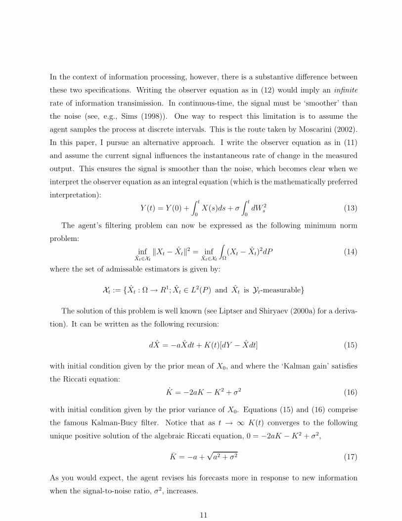
In the context of information processing, however, there is a substantive difference between
these two specifications. Writing the observer equation as in (12) would imply an infinite
rate of information transimission. In continuous-time, the signal must be ‘smoother’ than
the noise (see, e.g., Sims (1998)). One way to respect this limitation is to assume the
agent samples the process at discrete intervals. This is the route taken by Moscarini (2002).
In this paper, I pursue an alternative approach. I write the observer equation as in (11)
and assume the current signal influences the instantaneous rate of change in the measured
output. This ensures the signal is smoother than the noise, which becomes clear when we
interpret the observer equation as an integral equation (which is the mathematically preferred
interpretation):
Y (t) = Y (0) +∫ t
0X(s)ds+ σ
∫ t
0dW 2
s (13)
The agent’s filtering problem can now be expressed as the following minimum norm
problem:
infXt∈Xt
‖Xt − Xt‖2 = infXt∈Xt
∫Ω(Xt − Xt)
2dP (14)
where the set of admissable estimators is given by:
Xt := Xt : Ω → R1; Xt ∈ L2(P ) and Xt is Yt-measurable
The solution of this problem is well known (see Liptser and Shiryaev (2000a) for a deriva-
tion). It can be written as the following recursion:
dX = −aXdt+K(t)[dY − Xdt] (15)
with initial condition given by the prior mean of X0, and where the ‘Kalman gain’ satisfies
the Riccati equation:
K = −2aK −K2 + σ2 (16)
with initial condition given by the prior variance of X0. Equations (15) and (16) comprise
the famous Kalman-Bucy filter. Notice that as t → ∞ K(t) converges to the following
unique positive solution of the algebraic Riccati equation, 0 = −2aK −K2 + σ2,
K = −a+√a2 + σ2 (17)
As you would expect, the agent revises his forecasts more in response to new information
when the signal-to-noise ratio, σ2, increases.
11
3.2 Robust Filtering
The previous analysis was based on the assumption that the model was correctly specified,
and the agent knew this. What if this isn’t the case? What if the agent entertains doubts
about the model? The presumed linear law of motion for the unobserved state variable,
X(t), might not only be a poor approximation, but the nature of the misspecification could
well be difficult to diagnose. This wouldn’t be a serious problem if Kalman filters were robust
to such misspecification. Unfortunately, this isn’t the case. (See Petersen and Savkin (1999)
for examples).
In response to this lack of robustness, engineers have devised control and filtering methods
that are more robust to misspecification. The breakthrough came in the control context,
with the work of Zames (1981), who showed how to derive policies that guarantee a given
performance level. His idea was to switch objective functions, from the H2 sum-of-squares
norm to the H∞ supremum norm. Rather than optimize the average behavior of a system
based on a presumed statistical model for the disturbances, H∞-control and filtering is based
on a deterministic, worst-case analysis of the disturbances. This permits a model’s error
term to capture a complex amalgam of potential misspecifications, e.g., omitted variables,
neglected nonlinearities, or misspecified statistical distributions.
Recently, Hansen and Sargent (2002) have begun to import and adapt these methods to
economics. Although the formal decision theory justifying their use in economics remains
the subject of some dispute (see, e.g., the debate between Epstein and Schneider (2001) and
Hansen, Sargent, Turmuhambetova, and Williams (2001)), the hope is that robust control
offers a convenient dynamic extension of Gilboa and Schmeidler’s (1989) axiomatization of
Knightian Uncertainty. This axiomatization is motivated by the desire to explain experi-
mental findings that apparently violate Savage’s axioms, especially the Ellsberg Paradox.
Gilboa and Schmeidler show that the Ellsberg Paradox can be resolved if the ‘Sure Thing
Principle’ is relaxed.12
One aspect of the engineering approach to robust control and filtering that economists
have had to modify is its deterministic interpretation of a model’s disturbance process.
Deterministic errors produce stochastic singularities and make it difficult to compare models.
Engineers don’t need to worry about this since the appropriate degree of robustness is usually
dictated by externally imposed performance or stress requirements. In economics, however,
12The Sure Thing Principle is the analog of the independence axiom in models of subjective probability.
12

agents presumably get to decide the appropriate degree of robustness based on observations
of historical data. The greater the range of potential models that are consistent with the
data, the greater the degree of model uncertainty.
A stochastic approach to model uncertainty has been developed by Anderson, Hansen,
and Sargent (2003).13 In this approach model uncertainty is introduced by thinking of the
agent as being unsure about the true probability measure generating the data. Equations
(10) and (11) now constitute only a benchmark, or reference, probability measure around
which a class of perturbed probability measures are contemplated. The distance between
the reference model and the alternatives is measured by their relative entropies:
Definition 1: Let (Ω,F) be a measurable space, and let M(Ω) be a set of probability measures
on (Ω,F). Given any two probability measures Q,P ∈ M(Ω), the relative entropy of the
probability measure Q with respect to the probability measure P is defined by:
h(Q‖P ) :=
∫log
(dQdP
)dQ if Q P
+∞ otherwise
where Q P denotes absolute continuity of the measure Q with respect to the measure P,
and dQdP
is the Radon-Nikodym derivative of Q with respect to P.
Hence, relative entropy is akin to a log-likelihood ratio statistic. The absolute continuity
condition implies that Q and P share the same measure zero events. This is a reasonable
condition to impose on the set of admissable perturbations. If they weren’t absolutely
continuous, they would be easy to distinguish.
A key advantage of measuring model uncertainty by relative entropy is that Girsanov’s
Theorem delivers a very convenient parameterization of the alternative models. Let (ξi(t),Ft),
0 ≤ t ≤ T be a random process satisfying the following (Novikov) conditions:
P
(∫ T
0|ξi(s)|2ds <∞
)= 1
EP exp
(1
2
∫ T
0|ξi(s)|2ds
)< ∞
From this process, construct the following process,
ζi(t) = exp(∫ t
0ξi(s)dWs − 1
2
∫ t
0|ξi(s)|2ds
)13Interestingly, engineers are starting to adopt a stochastic approach as well. In fact, the robust filtering
approach of Petersen and Ugrinovskii (2002) is actually closer to my approach than is Anderson et. al.(2003).
13
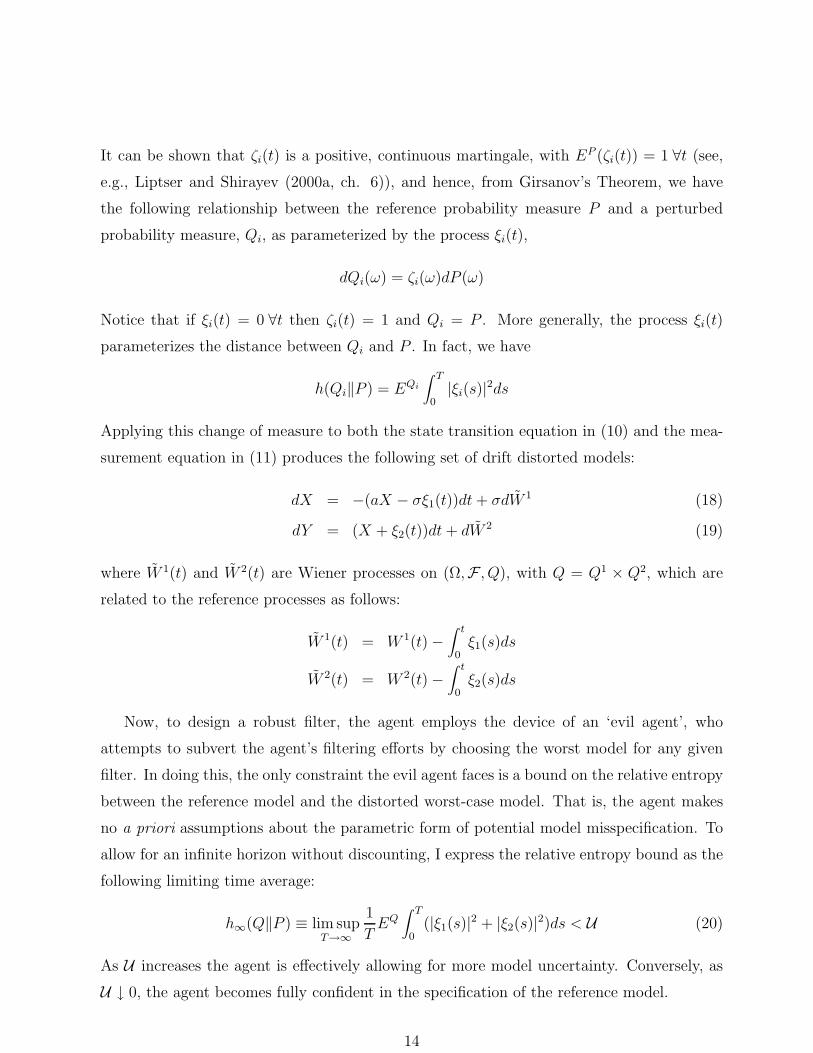
It can be shown that ζi(t) is a positive, continuous martingale, with EP (ζi(t)) = 1 ∀t (see,
e.g., Liptser and Shirayev (2000a, ch. 6)), and hence, from Girsanov’s Theorem, we have
the following relationship between the reference probability measure P and a perturbed
probability measure, Qi, as parameterized by the process ξi(t),
dQi(ω) = ζi(ω)dP (ω)
Notice that if ξi(t) = 0 ∀t then ζi(t) = 1 and Qi = P . More generally, the process ξi(t)
parameterizes the distance between Qi and P . In fact, we have
h(Qi‖P ) = EQi
∫ T
0|ξi(s)|2ds
Applying this change of measure to both the state transition equation in (10) and the mea-
surement equation in (11) produces the following set of drift distorted models:
dX = −(aX − σξ1(t))dt+ σdW 1 (18)
dY = (X + ξ2(t))dt+ dW 2 (19)
where W 1(t) and W 2(t) are Wiener processes on (Ω,F , Q), with Q = Q1 × Q2, which are
related to the reference processes as follows:
W 1(t) = W 1(t) −∫ t
0ξ1(s)ds
W 2(t) = W 2(t) −∫ t
0ξ2(s)ds
Now, to design a robust filter, the agent employs the device of an ‘evil agent’, who
attempts to subvert the agent’s filtering efforts by choosing the worst model for any given
filter. In doing this, the only constraint the evil agent faces is a bound on the relative entropy
between the reference model and the distorted worst-case model. That is, the agent makes
no a priori assumptions about the parametric form of potential model misspecification. To
allow for an infinite horizon without discounting, I express the relative entropy bound as the
following limiting time average:
h∞(Q‖P ) ≡ lim supT→∞
1
TEQ
∫ T
0(|ξ1(s)|2 + |ξ2(s)|2)ds < U (20)
As U increases the agent is effectively allowing for more model uncertainty. Conversely, as
U ↓ 0, the agent becomes fully confident in the specification of the reference model.
14

A robust filter can now be characterized as the Nash equilibrium of the following dynamic
zero-sum game,14
Vt = infXs
supQ
lim supT→∞
1
2TEQ
∫ T
0|Xs − Xs|2ds− 1
2θh∞(Q‖P )
(21)
subject to the distorted model in (18) and (19). The parameter θ can be interpreted as a
Lagrange Multiplier on the relative entropy constraint in (20). (As noted by Hansen and
Sargent (2002), we can omit the θU term since it does not influence behavior). Hence, θ
indexes the degree of robustness. As θ increases, robustness decreases. In the limit, as
θ → ∞, the problem becomes identical to the standard Kalman-Bucy filtering problem
studied in the previous section. Conversely, the smallest value of θ that is consistent with
the existence of a bounded solution to (21) can be interpreted as a stochastic H∞ filter,
providing the maximal degree of robustness for a given reference model. As emphasized by
Anderson, Hansen, and Sargent (2003) this may or may not be an empirically plausible filter.
If the implied detection error probability is regarded as being implausibly low, then θ should
be increased.
Before computing the equilibrium of this game there is an important feature of (21) that
should be highlighted. Notice that the lower limit of integration in (21) is 0, not t, implying
the agent cares about past forecast errors. Whether this is reasonable is likely to be case
specific. As noted by Hansen and Sargent (2002), assuming agents care about past forecast
errors is reasonable when agents must commit in advance to a given filter. On the other
hand, if agents ignore past forecast errors, letting bygones be bygones, then it turns out that
the standard Kalman filter is robust, in the sense that it minimizes the maximum one-step
ahead forecast error.15 In the next section we’ll see that a nonrecursive robust filter can be
interpreted as requiring extra information processing. This suggests that when agents must
commit in advance to a filter they will allocate more information processing to the task.
When solving the robust filtering problem in (21) it proves convenient to exploit the
following Legendre-type duality relationship between relative entropy and a risk-sensitive
version our criterion function:
14Hansen and Sargent (2002) call this the ‘multiplier game’, while Basar and Bernhard (1995) call it the‘soft-constrained game’.
15See Hansen and Sargent (2002) or Basar and Bernhard (1995, ch. 7) for a proof. This result is perhapsmost easily understood in the frequency domain. A recursive robust filter minimizes the maximum of thespectral density of one-step ahead forecast errors. However, by construction, the Kalman filter produces awhite noise forecast error, which is flat already, and hence, maximally robust.
15

Lemma 3.1: Let P ∈ M(Ω), and ψ : Ω → R1 be a measurable function. Then for every
Q ∈ M(Ω) we have the following Legendre transform relationships between h(Q‖P ) and the
log moment generating function of ψ:
h(Q‖P ) = supψ∈B(Ω)
∫ψdQ− log
(∫eψdP
)(22)
log(∫
eψdP)
= supQ∈M(Ω)
∫ψdQ− h(Q‖P )
(23)
where B(Ω) denotes the set of bounded F-measurable functions on Ω.
This duality relationship is useful because it allows us to transform our entropy con-
strained robust filtering problem into an equivalent risk-sensitive control problem. In partic-
ular, we shall use the version in (23) with ψ ≡ (Xs − Xs)2 to replace the ‘inner part’ of the
minmax filtering problem with a conventional risk-sensitive objective function. Although
the ψ function in our case is quadratic, and hence unbounded, Dai Pra, Meneghini, and
Runggaldier (1996) show that the duality in lemma 3.1 can be extended to cover this case
as well. Solving the resulting risk-sensitive filtering problem yields,
Proposition 3.1: If θ > 1 there is a unique solution of the the robust filtering problem in
(21) given by
dX = −aXdt+Kr(t)[dY − Xdt] (24)
Kr = −2aKr −(1 − 1
θ
)K2r + σ2 (25)
where the robust Kalman gain, Kr(t), converges to the following solution of the algebraic
Riccati equation, Kr = 0:
Kr =−a+
√a2 + (1 − θ−1)σ2
1 − θ−1(26)
If θ < 1 there does not exist a solution of the robust filtering problem.
Proof: To prove this we can follow Ugrinovskii and Petersen (2002). The basic idea is to scale
both sides of (23) by θ, and then define ψ = θψ. The right-hand side becomes an entropy
constrained filtering problem in terms of the scaled objective function, ψ. The left-hand sidebecomes a risk-sensitive control problem, also in terms of ψ, with risk-sensitivity parameter1/θ. The solution of this problem is a special case of Theorem 3 in Pan and Basar (1996).
There are a couple of interesting things to note about the robust Kalman gain in (26).
First, it is identical to the robust filter in Theorem 7.6 of Basar and Bernhard (1995),
16

which is based on a deterministic interpretation of the disturbances. Hence, adopting a
stochastic approach does not produce different results, but it does aid in the calibration of
the θ parameter. Second, comparing (26) to the standard Kalman gain in (17) reveals, as
expected, that Kr → K when θ → ∞. More generally, we have:
Corollary 3.1: The gain of the robust filter increases with model uncertainty.
Proof: Differentiate (26) with respect to θ and verify ∂Kr/∂θ < 0.
Since this is the main result from the perspective of relating robustness and information
processing, it is useful to have some intuition for it. To do this, suppose for simplicity that
the state transition equation is the only source of uncertainty, so that ξ2(t) = 0 ∀t. Also,
without loss of generality (see, Hansen and Sargent (2002)), confine attention to a Markov
Perfect Nash equilibrium in which the filterer selects a feedback rule (ie., a Kalman gain
parameter, K) at the same time his evil agent selects a feedback rule for ξ1(t) = Ge(t),
where e(t) is the forecast error (X − X). Given choices of K and G we get the following
Ornstein-Uhlenbeck process for the forecast errors:
de = −(a− σG+K)edt+ σdW1 −KdW2
which produces the following expression for the steady state variance of the forecast error:
var(e) =σ2 +K2
2(a− σG+K)
Subtracting the relative entropy constraint, θG2var(e), and then differentiating with respect
to K and G yields the following two reaction functions:
K(G) : 2K(a− σG+K) = σ2 +K2 (27)
G(K) : σG = (a+K) −√
(a+K)2 − σ2/θ (28)
These two functions are plotted in Figure 1.16 Starting at the standard Kalman gain, the evil
agent can produce a higher forecast error variance by choosing a disturbance process that
feeds back positively on e. This increases the persistence and variance of the forecast errors.
To ward off this possibility, the agent picks a higher, more vigilant, gain parameter. This
16Note, figure 1 just depicts the essential aspects of the situation. K(G) is actually concave (when K ison the horizontal axis) and G(K) is convex.
17

makes him less susceptible to low frequency misspecifications, which are especially damaging.
The agent raises the gain parameter up until the point that an evil agent would no longer
have an incentive to increase the persistence of the forecast errors. Clearly, making the evil
agent’s actions more costly by increasing θ causes the G(K) reaction function to shift down
and to the left (as well as becoming flatter). This allows the agent to relax a bit and reduce
the filter gain.
A natural question at this point is whether there is any evidence of heightened sensitivity
to prediction errors in the presence of model uncertainty. Unfortunately, while there is a
vast psychology literature debating whether agents update according to Bayes Rule, it does
not directly examine the effects of model uncertainty. The early literature actually found
evidence of conservatism (Edwards (1968)). In what is perhaps the only analysis of the
implications of model uncertainty for Bayesian updating, Navon (1978) argued that apparent
conservatism could be explained if agents suspect the data are subject to measurement error
or mean reversion. While this would indeed rationalize conservative updating, it would not
be robust. An agent with a preference for robustness should be concerned that the data are
less mean reverting than it appears. Failure to respond to hidden persistence is far more
costly than failure to detect mean reversion. As it turns out, however, the recent literature
has focused much more on the tendency of agents to overreact to new information in a variety
of settings (e.g., Kahneman and Tversky (1973) and Grether (1980)). This should probably
not be construed as evidence in favor of robust filtering, however, since this same evidence
points to more radical departures from Bayesian updating. At this point all one can safely
conclude is that the jury is still out.17
3.3 Capacity Constrained Filtering
Let’s now restore the agent’s faith in the model. Instead of being unsure about the model,
assume he has limits on his ability to process information. The objective is to formalize and
generalize the analysis of information processing that was presented earlier in the context
of Sims’ (2003) model of Rational Inattention. To do this we now regard the state space
model in (10) and (11) as an information transmission channel, with output Y and input
signal X. Our first task is to provide a rigorous definition of the information about X that
17Interestingly, Mullainathan (2002) shows that memory limitations can also produce overreaction toforecast errors. This occurs when new information triggers memories that convey similar information.
18
is contained in Y .
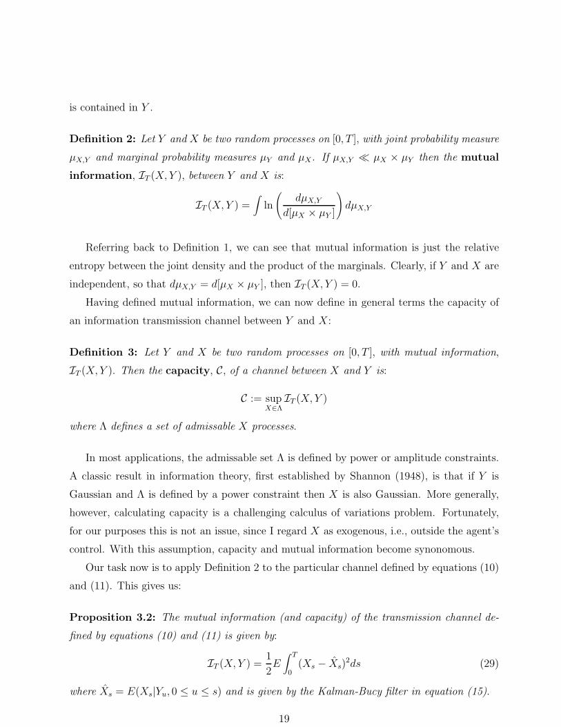
Definition 2: Let Y and X be two random processes on [0, T ], with joint probability measure
µX,Y and marginal probability measures µY and µX . If µX,Y µX × µY then the mutual
information, IT (X,Y ), between Y and X is:
IT (X,Y ) =∫
ln
(dµX,Y
d[µX × µY ]
)dµX,Y
Referring back to Definition 1, we can see that mutual information is just the relative
entropy between the joint density and the product of the marginals. Clearly, if Y and X are
independent, so that dµX,Y = d[µX × µY ], then IT (X,Y ) = 0.
Having defined mutual information, we can now define in general terms the capacity of
an information transmission channel between Y and X:
Definition 3: Let Y and X be two random processes on [0, T ], with mutual information,
IT (X,Y ). Then the capacity, C, of a channel between X and Y is:
C := supX∈Λ
IT (X,Y )
where Λ defines a set of admissable X processes.
In most applications, the admissable set Λ is defined by power or amplitude constraints.
A classic result in information theory, first established by Shannon (1948), is that if Y is
Gaussian and Λ is defined by a power constraint then X is also Gaussian. More generally,
however, calculating capacity is a challenging calculus of variations problem. Fortunately,
for our purposes this is not an issue, since I regard X as exogenous, i.e., outside the agent’s
control. With this assumption, capacity and mutual information become synonomous.
Our task now is to apply Definition 2 to the particular channel defined by equations (10)
and (11). This gives us:
Proposition 3.2: The mutual information (and capacity) of the transmission channel de-
fined by equations (10) and (11) is given by:
IT (X,Y ) =1
2E∫ T
0(Xs − Xs)
2ds (29)
where Xs = E(Xs|Yu, 0 ≤ u ≤ s) and is given by the Kalman-Bucy filter in equation (15).
19

Proof: For our special case of linear diffusion processes, this result was first proved by Duncan(1970). However, I follow the proof in Liptser and Shiryaev (2000b, ch. 16). The details arein the appendix.
As you would expect from standard signal extraction logic, the information in Y about
X is an increasing function of the conditional variance of X. For example, if the conditional
variance of X is small then movements in Y likely reflect measurement error, and do not
convey much information about X. We can use this result along with equation (17) to derive
the following expression for the asymptotic rate of information flow (per unit time) in terms
of the steady state Kalman gain:
Corollary 3.2: The steady state rate of information conveyed by Y about X is given by
limT→∞
1
TIT (X,Y ) =
1
2K =
1
2(−a+
√a2 + σ2)
Proof: K(T ) converges to K as T → ∞.
If we now denote channel capacity by κ, the information processing constraint simply
becomes K < 2κ. There is certainly no guarantee that this be binding. If the parameters
are such that the optimal Kalman gain satisfies this constraint then information processing
constraints are irrelevant. Since for our purposes this is not an interesting case, in what
follows I make the following assumption about the parameters:
Assumption 1: The parameter values satisfy the inequality, κ < 12(−a+
√a2 + σ2)
Hence, decisions characterized by a low signal-to-noise ratio are assumed to have a low
channel capacity. Not only is this a reasonable assumption, but it is likely to be the equi-
librium outcome in any problem permitting the endogenous allocation of capacity across
multiple decisions (eg., Turmuhambetova (2003)).
If Assumption 1 holds then we get the following characterization of capacity constrained
filtering.
Proposition 3.3: If Assumption 1 holds then the filter gain is 2κ, and an increase in channel
capacity increases the filter gain.
Proof: If Assumption 1 holds then the capacity constraint binds. Since the loss function is
20
globally convex with a minimum at (−a +√a2 + σ2), if the constraint is binding then it is
optimal to increase the filter gain in response to an increased channel capacity.
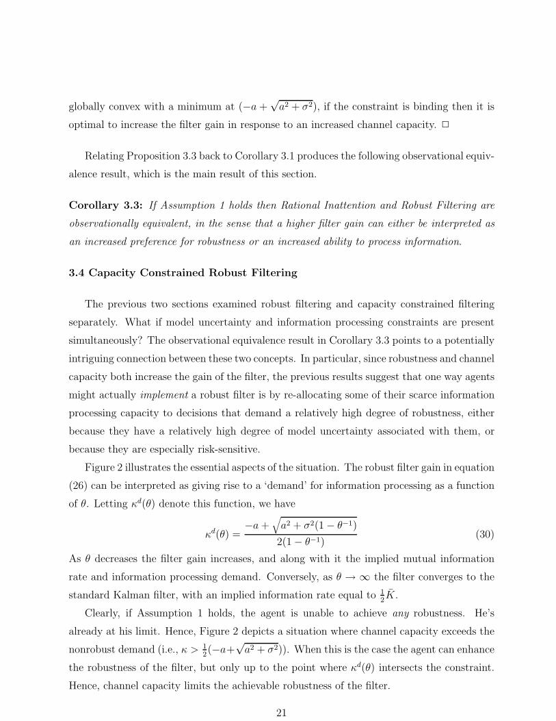
Relating Proposition 3.3 back to Corollary 3.1 produces the following observational equiv-
alence result, which is the main result of this section.
Corollary 3.3: If Assumption 1 holds then Rational Inattention and Robust Filtering are
observationally equivalent, in the sense that a higher filter gain can either be interpreted as
an increased preference for robustness or an increased ability to process information.
3.4 Capacity Constrained Robust Filtering
The previous two sections examined robust filtering and capacity constrained filtering
separately. What if model uncertainty and information processing constraints are present
simultaneously? The observational equivalence result in Corollary 3.3 points to a potentially
intriguing connection between these two concepts. In particular, since robustness and channel
capacity both increase the gain of the filter, the previous results suggest that one way agents
might actually implement a robust filter is by re-allocating some of their scarce information
processing capacity to decisions that demand a relatively high degree of robustness, either
because they have a relatively high degree of model uncertainty associated with them, or
because they are especially risk-sensitive.
Figure 2 illustrates the essential aspects of the situation. The robust filter gain in equation
(26) can be interpreted as giving rise to a ‘demand’ for information processing as a function
of θ. Letting κd(θ) denote this function, we have
κd(θ) =−a+
√a2 + σ2(1 − θ−1)
2(1 − θ−1)(30)
As θ decreases the filter gain increases, and along with it the implied mutual information
rate and information processing demand. Conversely, as θ → ∞ the filter converges to the
standard Kalman filter, with an implied information rate equal to 12K.
Clearly, if Assumption 1 holds, the agent is unable to achieve any robustness. He’s
already at his limit. Hence, Figure 2 depicts a situation where channel capacity exceeds the
nonrobust demand (i.e., κ > 12(−a+
√a2 + σ2)). When this is the case the agent can enhance
the robustness of the filter, but only up to the point where κd(θ) intersects the constraint.
Hence, channel capacity limits the achievable robustness of the filter.
21

4 Using Channel Capacity to Parameterize a Prefer-
ence for Robustness
One common criticism of robust control and filtering is that it imputes an excessive degree
of pessimism to agents. Why base decisions on the worst potential outcome? Didn’t Savage
show that even when events are unique and nonreplicable we can still model agents as if they
were formulating subjective probabilities over them and maximizing expected utility?
To a Bayesian this is the end of the story.18 To make sense of robust control and filtering
you must doubt the validity of the Savage axioms. Cause for doubt has come on two fronts.
First, a growing experimental literature has repeatedly confirmed and generalized the results
of the Ellsberg paradox, which is fundamentally in conflict with the existence of a (unique)
subjective prior probability distribution. Second, and perhaps more persuasive to those
who doubt the generality of experimental results, models which incorporate a preference
for robustness seem better able to explain observed market data, particularly asset market
data.19
Of course, a Bayesian response to these results is: How could they do worse? Robust
control and filtering models come with an extra free parameter (i.e., θ) that can be tuned
to explain anything. Hence, to make robust control methods persuasive it is essential that
some discipline be placed on the calibration of θ. Setting θ too low can indeed produce an
excessive degree of pessimism.
Fortunately, Anderson, Hansen, and Sargent (2003) have developed a useful strategy
for calibrating this parameter. Their strategy exploits a connection between the worst-
case shocks and conditional relative entropy on the one hand, and a connection between
conditional relative entropy and Bayesian detection error probabilities on the other hand.
Given a prior about what constitutes a reasonable detection error probability, they show
how to back out a value for θ that generates this probability. With this methodology, one
can set θ so that agents only hedge against models that could have plausibly generated past
observed data. This disciplines the choice of θ, and answers the criticism that a minimax
objective makes people unduly pessimistic.
18See Sims (2001) for a critique of robust control along standard Bayesian lines. He argues that while aminimax approach might provide a convenient method for generating a useful prior in some applications, itshould not be regarded as a normative decision theory.
19See, e.g., Hansen, Sargent, and Tallarini (1999) and Anderson, Hansen, and Sargent (2003), and thereferences they provide.
22

Interestingly, information processing constraints suggest an alternative, complementary
strategy for calibrating θ. If we actually knew what channel capacity was then equation (30)
would deliver an immediate parameterization of θ, as long as we assumed that the capacity
constraint was binding. Unfortunately, as noted earlier, it is not likely that we could ever
expect to measure directly and persuasively a generally applicable value of κ. This hope was
pretty much dead by the early 1960s.20 However, I will now argue that we can exploit the
insights of Anderson, Hansen, and Sargent (2003) to devise an indirect strategy for linking
θ to channel capacity.
The calibration consists of two steps. The first step is to relate channel capacity to
detection error probabilities. This can be done using the results of Kailath (1969) and Evans
(1974). The second step is to then use equation (30) to link κ to θ. Hence, as in Anderson,
Hansen, and Sargent (2003), we can calibrate θ to detection error probabilities, but we do
so through the intermediate step of relating each to channel capacity. As long as you are
willing to assume the capacity constraint binds, this indirect strategy can provide some
computational advantages.
To see this, let’s start with Kailath’s (1969) expression for the likelihood ratio between
the following two diffusion processes:
H0 : dY = X0tdt+ dWt
H1 : dY = X1tdt+ dWt
where our task is to decide which of the two unobserved diffusion processes, X0t or X1t, is
generating the observed Y data. The likelihood ratio can be written as follows:
LR ≡ Λ(T ) = exp
∫ T
0(X1t − X0t)dY − 1
2
∫ T
0(X2
1t − X20t)dt
(31)
where Xit is a Yt-measurable least squares estimate of Xit assuming that hypothesis Hi is
true. These too are diffusions, generated by the Kalman-Bucy filter derived in section 3.1.
Given this, the decision rule is standard:
(T ) ≡ ln Λ(T ) < γ ⇒ H1
> γ ⇒ H0
20Despite this, a still active subfield in psychology (i.e., psychophysics) continues to provide measures ofchannel capacity in very specific, narrowly defined contexts.
23

where γ is a threshold determined by the relative importance of Type I and Type II errors.
In what follows, I treat the two errors symmetrically and set γ = 0.
In principle, we could at this point derive a diffusion process for (T ) and calculate the
probabilities that (T ) < 0 when H0 is true and (T ) > 0 when H1 is true. This would give
us the overall detection error probability. Unfortunately, exact expressions are hard to come
by. In practice, it is much easier to calculate bounds on the detection errors. Essentially, we
need to calculate the probability that a diffusion with positive drift ends up at a negative
value. This is a ‘large deviations’ problem, with the escape probability being an exponentially
decreasing function of the sample size and a ‘rate function’ determined by the parameters of
the problem. This is basically the route taken by Evans (1974), although he works with the
Fokker-Planck equation for the moment generating function of (T ) rather than its Legendre
transform.
Specifically, if we define the moment-generating function of (T ) as follows,
Mi(s) = Eexp[s(T )|Hi] = E[Λ(T )s|Hi]
then a standard Chernoff bound calcuation yields,
P (error|Hi) ≤Mi(s)
The trick is to evaluate Mi(s). By first writing the prediction error decompositions of Y
under each hypothesis, and then substituting into (31), we get:
Λst ≡ φ(t) = exp
[s∫
(X1t − X0t)dv − s
2
∫(X1t − X0t)
2dt]
where dv is a Brownian motion prediction error process. Applying Ito’s lemma to this yields:
dφ =s2 − s
2(X1t − X0t)
2φdt+ s(X1t − X0t)φdv (32)
Using (32) along with the hypothesized diffusions for X1 and X2 delivers
MT (s) = exp
[s2 − s
2
∫ T
0P (t)dt
]
where P (t) is the solution of a Riccati equation. Finally, noting that s = 1/2 is the bound-
minimizing choice of s, and letting T → ∞ gives us the following detection error probability:
P (error) ≤ exp[−1
8P∞T
](33)
24

where P∞ is the steady state value of P (t).
Now the punch-line is that by following the logic of section 3.3 we can regard P∞ as the
capacity of a re-defined information transmission channel. As this capacity increases the
maximal detection error probability decreases. This suggests an upper bound on P∞ which,
from (30), implies a lower bound on θ (assuming κd(θ) < P∞). Notice that we have not had
to calculate relative entropy as a function θ. Although it’s lurking in the background as an
element of P∞, as long as we assume that channel capacity is binding we do not have to
explicitly calculate it. This may be advantageous in some applications.
5 Conclusion
This paper has illustrated some potential connections between Robust Filtering and Ratio-
nal Inattention. It has shown that under certain conditions a greater responsiveness to new
information can either be interpreted as an increased concern for robustness in the presence
of model uncertainty, or an increase in information processing ability when agents are re-
garded as finite capacity information transmission channels. By making these connections,
this paper raises questions about the deeper psychological links between uncertainty and
information processing. Following up on the early work of Kahneman (1973), perhaps one
way agents actually formulate and implement robust policies is by reallocating their limited
channel capacity to highly uncertain or risk-sensitive situations.
Besides exploring these links in greater detail, there are a number of other more straight-
forward extensions that could be pursued in future work. First, while it is usually the case
that there is little conceptual loss of generality in confining attention to univariate cases,
that is not true in models of Rational Inattention. As noted by Sims, and discussed in more
detail by Kahneman, with Rational Inattention there may be possibilities to reallocate ca-
pacity among variables, and focus attention where it has the greatest payoff. This calls for
a multivariate extension of these results. Second, this paper has focused on filtering and ab-
stracted from control. Information processing constraints also have implications for control
that merit future research. As noted by Hansen and Sargent (2002) and Basar and Bernhard
(1995), with model uncertainty the usual separation between filtering and control no longer
applies, and it is likely that information processing constraints also produce some interest-
ing interactions between these two problems. In addition to the work of Sims, interesting
starts along this dimension have been made by Turmuhambetova (2003) and Kuznetsov,
25

Liptser, and Serebrovskii (1980). Finally, the observational equivalence derived here bears
some resemblance to the result of Hansen, Sargent, and Tallarini (1999). They showed in
the context of a Permanent Income model that the quantity implications of robustness are
observationally equivalent to a reduced rate of time preference. They argue that the effects
of robustness and model uncertainty manifest themselves most clearly in asset prices. This
suggests that information processing constraints might also have important implications for
security market data and the resolution of various asset price anomalies.
26

APPENDIX
This appendix fills in some of the details of the proof of Proposition 3.2. First, one canreadily verify that equations (10) and (11) satisfy conditions (A) - (E) in chapter 7 of Liptserand Shiryaev (2000a).21 Given this, the fact that µX,Y µX × µW and µY µW implies
dµX,Yd[µX × µY ]
=dµX,Y /d[µX × µW ]
dµY /dµW(A1)
Next, we can apply lemmas 7.6 and 7.7 in Lipster and Shiryaev (2000a) to conclude,
dµX,Yd[µX × µW ]
= exp
[∫ T
0XtdYt − 1
2
∫ T
0X2t dt
](A2)
dµYdµW
= exp
[∫ T
0XtdYt − 1
2
∫ T
0X2t dt
](A3)
Substituting (A2) and (A3) into (A1) yields,
lndµX,Y
d[µX × µY ]=
∫ T
0[Xt − Xt]dYt − 1
2
∫ T
0[X2
t − X2t ]dt
=∫ T
0
([Xt − Xt]Xt − 1
2[X2
t − X2t ])dt+
∫ T
0[Xt − Xt]dWt (A4)
Finally, taking expectations in (A4), collecting terms, and exploiting the properties ofstochastic integrals to eliminate the last term in (A4) yields,
E
[ln
dµX,Yd[µX × µY ]
]=
1
2E∫ T
0(Xt − Xt)
2dt
21These conditions include the following: (A), existence of a strong (i.e., FX,Wt -measurable) solution of
(11); (B), Nonanticipative drift and diffusion coefficients in (11); (C), A growth condition on the diffusioncoefficient in (11) (satisfied trivially here); and boundedness assumptions on the drift term in (11). Actually,since W 2 and X are assumed independent, we can (from the note to Theorem 7.23 in Lipster and Shiryaev)dispense with conditions (A) and (C).
27

28

29

REFERENCES
Allport, D.A., B. Antonis, and P. Reynolds, 1972, On the Division of Attention: A Disproofof the Single Channel Hypothesis, Quarterly Journal of Experimental Psychology 24,225-35.
Anderson, Evan W., Lars P. Hansen, and Thomas J. Sargent, 2003, A Quartet of Semigroupsfor Model Specification, Robustness, Prices of Risk, and Model Detection, mimeo,University of Chicago.
Basar, Tamer, and Pierre Bernhard, 1995, H∞-Optimal Control and Related MinimaxDesign Problems: A Dynamic Game Approach, 2nd Edition, Boston-Basel-Berlin:Birkhauser.
Broadbent, Donald E., 1958, Perception and Communication, London: Pergamon.
Cover, Thomas M., and Joy A. Thomas, 1991, Elements of Information Theory, John Wiley& Sons, Inc.
Dai Pra, P., L. Meneghini, and W. Runggaldier, 1996, Connections Between StochasticControl and Dynamic Games, Mathematics of Control, Systems, and Signals 9, 303-26.
Duncan, Tyrone E., 1970, On the Calculation of Mutual Information, SIAM Journal ofApplied Mathematics 19, 215-20.
Edwards, Ward, 1968, Conservatism in Human Information Processing, in B. Kleinmuntz,ed., Formal Representation of Human Judgment, Wiley & Sons.
Epstein, Larry G., and Martin Schneider, 2001, Recursive Multiple-Priors, mimeo, Univer-sity of Rochester.
Evans, James E., 1974, Chernoff Bounds on the Error Probability for the Detection ofNon-Gaussian Signals, IEEE Transactions on Information Theory 20, 569-77.
Gilboa, Itzhak, and David Schmeidler, 1989, Maximin Expected Utility with Non-uniquePrior, Journal of Mathematical Economics 18, 141-53.
Grether, David M., 1980, Bayes’ Rule as a Descriptive Model: The RepresentativenessHeuristic, Quarterly Journal of Economics 95, 537-57.
Hansen, Lars P., and Thomas J. Sargent, 2002, Robust Control and Economic Model Un-certainty, forthcoming monograph.
Hansen, Lars P., Thomas J. Sargent, and Thomas D. Tallarini, 1999, Robust PermanentIncome and Pricing, Review of Economic Studies 66, 873-907.
Hansen, Lars P., Thomas J. Sargent, Gauhar A. Turmuhambetova, and Noah Williams,2000, Robustness and Uncertainty Aversion, mimeo, University of Chicago.
Kahneman, Daniel, 1973, Attention and Effort, Prentice-Hall, Inc.
Kahneman, Daniel, and Amos Tversky, 1973, On the Psychology of Prediction, Psycholog-ical Review 80, 237-51.
Kailath, Thomas, 1969, A General Likelihood-Ratio Formula for Random Signals in Gaus-sian Noise, IEEE Transactions on Information Theory 15, 350-61.
30
Kuznetsov, N.A., R.S. Liptser, and A.P. Serebrovskii, 1980, Optimal Control and DataProcessing in Continuous Time, Avtomatika i Telemekhanika 10, 47-53.
Liptser, Robert S., and A.N. Shiryaev, 2000a, Statistics of Random Processes I: GeneralTheory, Second Edition, Springer-Verlag.
, 2000b, Statistics of Random Processes II: Applications, Second Edition,Springer-Verlag.
Marschak, Jacob, 1971, Economics of Information Systems, Journal of the American Sta-tistical Association 66, 192-219.
Miller, George A., 1956, The Magic Number Seven, Plus or Minus Two: Some Limits onour Capacity for Processing Information, Psychological Review 63, 81-97.
Moray, N., 1967, Where is Capacity Limited? A Survey and a Model, Acta Psychologica27, 84-92.
Moscarini, Giuseppe, 2002, Limited Information Capacity as a Source of Inertia, mimeo,Yale University.
Mullainathan, Sendhil, 2002, A Memory-Based Model of Bounded Rationality, QuarterlyJournal of Economics 117, 735-66.
Navon, David, 1978, The Importance of Being Conservative: Some Reflections on HumanBayesian Behavior, British Journal of Mathematical and Statistical Psychology 31, 33-48.
Pan, Zigang, and Tamer Basar, 1996, Model Simplification and Optimal Control of Stochas-tic Singularly Perturbed Systems Under Exponentiated Quadratic Cost, SIAM Journalon Control and Optimization 34, 1734-66.
Parasuraman, Raja, 1998, The Attentive Brain, MIT Press.
Petersen, Ian R., and A.V. Savkin, 1999, Robust Kalman Filtering for Signals and Systemswith Large Uncertainties, Birkhauser: Boston.
Petersen, Ian R., and V.A. Ugrinovskii, 2002, Robust Filtering of Stochastic UncertainSystems on an Infinite Time Horizon, International Journal of Control 75, 614-26.
Pierce, John R., 1980, An Introduction to Information Theory: Symbols, Signals and Noise,Second Edition, Dover.
Posner, Michael I., and S.J. Boies, 1971, Components of Attention, Psychological Review78, 391-408.
Sargent, Thomas J., 1993, Bounded Rationality in Macroeconomics, Oxford Univ. Press.
Shannon, Claude E., 1948, A Mathematical Theory of Communication, Bell System Tech-nical Journal 27, 379-423, 623-656.
Sims, Christopher A., 1998, Stickiness, Carnegie-Rochester Conference Series on PublicPolicy 49, 317-56.
, 2001, Pitfalls of a Minimax Approach to Model Uncertainty, AmericanEconomic Review 91, 51-54.
, 2003, Implications of Rational Inattention, Journal of Monetary Economics
Turmuhambetova, Gauhar A., 2003, Stochastic Control for Systems with Information Con-straints, mimeo, University of Chicago.
31

Wiener, Norbert, 1961, Cybernetics: or Control and Communication in the Animal and theMachine, 2nd Edition, MIT Press.
Zames, George, 1981, Feedback and Optimal Sensitivity: Model Reference Transformation,Multiplicative Seminorms, and Approximate Inverses, IEEE Transactions on Auto-matic Control 26, 301-20.
32