Robustifying Learnability

Robert J. Tetlow∗ Peter von zur Muehlen†

March 31, 2005

Abstract

In recent years, the learnability of rational expectations equilibria (REE) and de-terminacy of economic structures have rightfully joined the usual performance criteriaamong the sought-after goals of policy design. Some contributions to the literature,including Bullard and Mitra (2001) and Evans and Honkapohja (2002), have made sig-nificant headway in establishing certain features of monetary policy rules that facilitatelearning. However a treatment of policy design for learnability in worlds where agentshave potentially misspecified their learning models has yet to surface. This paper pro-vides such a treatment. We begin with the notion that because the profession has yet tosettle on a consensus model of the economy, it is unreasonable to expect private agentsto have collective rational expectations. We go further in assuming that agents haveonly an approximate understanding of the workings of the economy and that their taskof learning true reduced forms of the economy is subject to potentially destabilizingerrors. The issue is then whether a central bank can design policy to account for errorsin learning and still assure the learnability of the model. Our test case is the standardNew Keynesian business cycle model. For different parameterizations of a given policyrule, we use structured singular value analysis (from robust control theory) to find thelargest ranges of misspecifications that can be tolerated in a learning model withoutcompromising convergence to an REE.In addition, we study the cost, in terms of performance in the steady state of a

central bank that acts to robustify learnability on the transition path to REE.

• JEL Classifications: C6, E5.• Keywords: monetary policy, learning, E-stability, learnability, robust control.

PRELIMINARY VERSION

∗Contact author: Robert Tetlow, Federal Reserve Board, 20th and C Streets, NW, Washington, D.C.20551. Email: rtetlow@frb.gov. We thank Brian Ironside for help with the charts. The views ex-pressed in this paper are those of the authors alone and do not represent those of the Board of Governorsof the Federal Reserve System or other members of its staff. This paper and others may be found athttp://www.members.cox.net/btetlow/default.htm

†von zur Muehlen & Associates, Vienna, VA 22181. E-mail: pvzmuehlen@cox.net

0

1 Introduction

It is now widely accepted that policy rules—and in particular, monetary policy rules—should

not be chosen solely on the basis of their performance in a given model of the economy.

There is simply too much uncertainty about the true structure of the economy to warrant

taking the risk of so narrow a criterion for selection. Rather, policy should be designed to

operate "well" in a wide range of models. There has been substantial progress in a relatively

short period of time in the literature on robustifying policy. The first strand of the literature

examines the performance of rules given the presence of measurement errors in either model

parameters or unobserved state variables.1 The second strand focuses on comparing rules in

rival models to see if their performance spanned reasonable sets of alternative worlds.2 The

third considers robustifying policy against unknown alternative worlds, usually by invoking

robust control methods.3

At roughly the same time, another literature was developing on the learnability (or E-

stability) of models.4 The learnability literature takes a step back from rational expectations

and asks whether the choices of uninformed private agents could be expected to lead to

converge on a rational expectations equilibrium (REE) as the outcome of a process of

learning. Important papers in this literature include Bray [5], Bray and Savin [6] and Marcet

and Sargent [34]. Evans and Honkapohja summarize some of their many contributions to

this literature in their book [18].

The question arises: could monetary policy help, or hurt, private agents learn the REE?

The common features of the robust policy literature include, first, that it is the government

that does not understand the true structure of the economy, and second, that the govern-

ment’s ignorance will not vanish simply with the collection of more data.5 By contrast, in the

1 Brainard [4] is the seminal reference. Among the many, more recent references in this large literatureare Sack [42], Orphanides et al. [39], Soderstrom [44] and Ehrmann and Smets [17].

2 See, e.g., Levin et al. [29] and [30].3 Hansen and Sargent [27] and [28], Tetlow and von zur Muehlen [47] and Coenen [13]. These strands of

the robustness literature are named in the text in chronological order but the three methods should be seenas complementary rather than substitutes.

4 In this paper, as in most of the rest of the literature, the terms learnability, E-stability and stabilityunder learning will all be used interchangeably. These terms are distinct from stable—without the "E-" or"under stability" added—which should be taken to mean saddle-point stable. The term saddle-point stable,determinate and regular are taken as equivalent adjectives describing equilibria.

5 The concept of "truth" is a slippery one in learning models. In some sense, the truth is jointly determinedby the deep structural parameters of the economy and what people believe them to be. Only in steady state,and then only under some conditions, will this be solely a function of deep parameters and not of beliefs.

1

learning literature it is usually the private sector that is assumed not to have the information

necessary to form rational expectations, but this situation has at least the prospect of being

alleviated with the passage of time and the collection of more data. In this paper, we take

the robust policy rules literature and marry it with the learnability literature.

Since the profession has been unable to agree on a generally acceptable workhorse model

of the economy, it is unreasonable to expect private agents to have rational expectations.

The most that one can expect is that agents have an approximate understanding of the

workings of the economy and that they are on a transition path toward learning the true

structure. This assumption we hold in common with those in the learning literature. From

a policy perspective, it follows that the job of facilitating that transition is logically prior to

the job of maximizing the performance of the economy once the transition is complete. In

this paper, we consider two issues. The first is how a policy maker might choose policy to

maximize the set of worlds occupied by private agents able to learn the REE. The second

is an assessment of the welfare cost of assuring learnability in terms of forgone stability in

equilibrium. Or, put differently, we measure the welfare cost of learnability insurance. Each

of these questions is important. In worlds of model uncertainty, an ill-chosen policy rule—

or policy maker—could lead to explosiveness or indeterminacy. At the same time, excessive

concern for learnability will imply costs in terms of forgone welfare.

Ours is not the first paper to consider the issue of choosing monetary policies for their abil-

ity to deliver determinacy and learnability. Bernanke and Woodford [2] argue that inflation-

forecast based policy rules—that is, those that feed back on forecasts of future output or

inflation—can lead to indeterminacy in linear rational expectations (LRE) models. Clarida,

Gali and Gertler [11] show that violation of the so-called Taylor principle in the context of

an IFB rule may have been the source of the inflation of the 1970s.6 Bullard and Mitra [8]

in an important paper show that higher persistence in instrument setting—meaning a large

coefficient on the lagged instrument in a Taylor-type rule—can facilitate determinacy in the

same class of models. Evans and Honkapohja [20] note similar problems in a wider class of

rules and argue for feedback on structural shocks, although questions regarding the observ-

Nevertheless, in this paper, when we refer to a "true model" or "truth" we mean the REE upon whichsuccessful learning eventually converges.

6 Levin et al. [30] and Batini and Pearlman [1] study the robustness properties of different types ofinflation-forecast based rules for their stability and determinacy properties.

2

ability of such shocks leave open the issue of whether such a policy is implementable. Evans

and McGough [22] compute optimal simple rules conditional on their being determinate in

rival models. Each of these papers makes an important contribution to the literature. But

all consider special cases within broader sets of policy choices. In this paper, we follow a

different approach and consider optimal policies to maximize learnability of the economy.

The remainder of the paper is organized as follows. The second section lays out the theory,

beginning with a review of the literature on least-squares learnability and determinacy, and

following with methods from the robust control literature. Section 3 blends the two together

to establish the tools with which we work. Section 4 contains our results. It begins with

our application of these methods to the case of the very simple Cagan model of money

demand in hyperinflations and then moves on to the New Keynesian business cycle (NKB)

model. For the NKB model, we study the design of time-invariant simple monetary policy

rules to robustify learnability of three types: a lagged-information rule, a contemporaneous

information rule and a forecast-based policy rule. And we close the section by covering the

insurance cost of robustifying learnability. A fifth and final section sums up and concludes.

2 Theoretical overview

2.1 Expectational equilibrium under adaptive learning

The theory of E-stability or learnability in linear rational expectations models dates back

more than 20 years to Bray [5] who showed that agents using recursive least squares would, if

the arguments to their regressions were properly specified, eventually converge on the correct

REE. This convergence property gave a considerable shot in the arm to rational expectations

applications since proponents had an answer to the question "how could people come to have

rational expectations?" The theory has been advanced by the work of Marcet and Sargent

[34] and Evans and Honkapohja [various]. Our rendition follows Evans and Honkapohja [18],

chapters 8-10.

Begin with the following linear rational expectations model:

Hyt = a+ FEtyt+1 + Lyt−1 +Gvt. (1)

3

At this point, Et represents a mathematical expectation conditioned on information avail-

able in period t. Later on, we shall distinguish between this rational expectation and an

expectation based on adaptive learning. Assuming the inverse of H exists, we re-write this

model as

yt = A+MEtyt+1 +Nyt−1 + Pvt, (2)

where yt is a vector of n endogenous variables, including, possibly, policy instruments, and vt

comprises allm exogenous variables. Equation (2) is general in that both non-predetermined

(or "jumper") variables, Etyt+1and predetermined variables, yt−1, are represented, and by

defining auxiliary variables, e.g., yjt = yt+j, j 6= 0, arbitrarily long (finite) lead or lag lengths

can be accommodated. It can also be easily extended to allow lagged expectations formation;

e.g., Et−1yt, and exogenous variables with some relatively minor changes in the results. Next,

define the prediction error for yt+1, to be t+1 = yt+1 −Etyt+1. Under rational expectations,

Et t+1 = 0, a martingale difference sequence. Evans and Honkapohja [18] show that for at

least one rational expectations equilibrium to exist, the stochastic process, yt, that solves

(2), must also satisfy:

yt+1 = aM−1 +M−1yt −M−1Nyt−1 −M−1Pvt + t+1 (3)

We can express (3) as a first-order system:

∙yt+1yt

¸=

∙aM−1

0

¸+

∙M−1 −NM−1

In 0

¸ ∙ytyt−1

¸+

∙−M−1

0

¸Pvt +

∙10

¸t+1 (4)

or, rewriting:

Yt+1 = A+BYt + Cvt +D t+1, (5)

where Y = [yt, yt−1]0. then we can easily show when (5) satisfies the Blanchard-Kahn [3]

conditions for stability, namely, that the characteristic roots of the matrix B of norm less

than unity equal the number of predetermined variables (taking yt to be scalar, this is one),

then the model is determinate, and there is just one martingale difference sequence, t+1,

that will render (3) stationary; if there are fewer roots inside the unit circle than there

are predetermined variables, the model is explosive meaning that there is no martingale

difference sequence that will satisfy the system; and if there are more roots inside the unit

4

circle than there are predetermined variables, the model is said to be indeterminate, and

there are infinite numbers of martingale difference sequences that make (3) stable. The

roots of B are determined by the solution to the characteristic equation: Ωλ2 − λ + δ = 0.

It follows that determinacy requires | δ + Ω |< 1.

Determinacy is one thing, learnability is quite another. As Bullard and Mitra [8] have

emphasized, determinacy does not imply learnability, and indeterminacy does not imply a

lack of learnability. We can address this question by postulating a representation for the REE

that a learning agent might use. For the moment, we consider the minimum state variable

(MSV) representation, advanced by McCallum [35]. Let us assume that vt is observable and

follows a first-order stochastic process,

vt = ρvt−1 + t, (6)

where t is an iid white noise process. The ρ matrix is assumed to be diagonal.

Under these assumptions, we can write the following perceived law of motion (PLM):

yt = a+ byt−1 + cvt. (7)

Rewrite equation (2) slightly, and designate expectations formed using adaptive learning

with a superscripted asterisk on the expectations operator, E∗t :

yt = A+ME∗t yt+1 +Nyt−1 + Pvt. (8)

Then, leading (7) one period, taking expectations, substituting (7) into the result, and finally

into (8), we obtain the actual law of motion, (ALM), the model under the influence of the

PLM :

yt = A+M(I + b)a+ (N +Mb2)yt−1 + (M(bc+ cρ) + P )vt. (9)

So the MSV solution will satisfy the mapping from PLM to ALM:

A+M(I + b)a = a, (10)

N +Mb2 = b, (11)

M(bc+ cρ) + P = c. (12)

Learnability depends then on the mapping of the PLM on to the ALM, defined from (9):

5

T (a, b, c) = [A+M(I + b)a,N +Mb2,M(bc+ cρ) + P ] (13)

The fixed point of this mapping is a MSV representation of a REE, and its convergence is

given by the matrix differential equation:

d

dτ(a, b, c) = T (a, b, c)− (a, b, c). (14)

Convergence is assured if certain eigenvalue conditions for the following matrix differential

equations are satisfied.

da

dτ= [A+M(I + b)]a− a, (15)

db

dτ= Mb2 +N − b,

dc

dτ= M(bc+ cρ) + P − c.

As shown by Evans and Honkapohja (2001), the necessary and sufficient conditions for E-

stability are that the eigenvalues of the following matrices have negative real parts:

DTa − I = M(I + b)− I, (16)

DTb − I = b0 ⊗M + I ⊗Mb− I, (17)

DTc − I = ρ0 ⊗M + I ⊗Mb− I. (18)

The important points to take from equations (15) are that the conditions are generally

multivariate in nature–meaning that the coefficients constraining the intercept term, a, can

be conflated with those of the slope term, b; and that the coefficients of both the PLM

and the ALM come into play. Learnability applications in the literature to date have been

to very simple, small-scale models where these problems rarely come into play.7 In the

kind of medium- to large-scale models that policy institutions use, these issues cannot be

safely ignored.8 In "real-world models", to the question of whether private agents know the

7 A notable exception is Garratt and Hall [23], but even then the learning problem was constrained toexchange rate determination. The rest of the London Business School model that they used was taken asknown.

8 At the Federal Reserve Board, for example, the staff use a wide range of models to analyze monetarypolicy issues, including a variety of reduced-form forecasting models, a calibrated multi-country DSGEmodel called SIGMA, a medium-scale DSGE U.S. model, and the FRB/US model, a larger-scale, partlymicro-founded estimated model.

6

model (or have to learn it) one needs to add the issue of whether the policy maker himself

knows the model. What properties should the selected policy rule have if the monetary

authority is unsure of the model under control? Without taking away anything from the

important contributions of Bullard and Mitra [8] and Evans and Honkapohja [20], the choice

of monetary policy rules must not only consider how they foster learnability in a given model

but whether they do so for the broader class of models within which the true model might

be found. Similarly, taking as given the true model, the initial beliefs of private agents

can affect learnability both through the inclusion and exclusion of states to the PLM and

through the initial values attached to parameters. In the context of the above example,

values of a, b, and c that are initially "too far" from equilibrium can block convergence. The

choice of a particular policy can shrink or expand the range of values for a, b, and c that is

consistent with E-stability.9 This is our concern in this paper: how can a policy maker deal

with uncertainty in the choice of his or her policy rule–uncertainty on his or her part and on

the part of the private sector–and maximize the probability that the economy will converge

successfully on a rational expectations equilibrium? For this, we work with perturbations to

the T-mapping described by equations (14) or systems like it. We take this up in the next

subsection.

2.2 Structured robust control

In the preceding subsection, we outlined the theory of least-squares learning in a relatively

general setting. In this subsection we review methods from robust control theory. Recall

that our objective is to uncover the conditions under which monetary policy can maximize

the prospect that the process of learning will converge on a REE–that is, to robustify

learnability–so the integration of the theories of these two subsections is what will provide

us with the tools we seek.

The argument that private agents might have to learn the true structure of the economy

takes a useful step back from the assumption of known and certain linear rational expecta-

tions models. However, what the literature to date has usually taken as given is, first, that

9 In fact, in this example, the intercept coefficient, a, turns out to be irrelevant for the determination oflearnability although this result is not general.

7

agents use least-squares learning to adapt their perceptions of the true economic structure,

and second, that they know the correct linear or linearized form of the REE solution.10 Both

of these assumptions can be questioned. It is a common-place convenience of macroecono-

mists to formulate a dynamic stochastic general equilibrium model and then linearize that

model. It is certainly possible that ill-informed agents use only linear approximations of their

true decision rules. But it is hard to argue that the linearized decision rule is any more valid

than some other approximation. Similarly, least-squares learning is the subject of research

more because of its analytical tractability than its veracity. The utility of tractable, linear

formulations of economic forms is undeniable. At the same time, however, the risk in over

reliance on such forms should be just as apparent. There would appear to be a least a prima

facie case for retaining the simplicity of linear state-space representations and linear rules,

while taking seriously the consequences of such approximations.

With this in mind, we retain the assumption of a linear reference model, and least-

squares learning on the part by agents, but assume that the process of learning is subject

to uncertainty. This may be because agents take their decision rules as simplifications of

truly optimal decision rules due to the complexity of such rules. Or it might be because our

assumption of least-squares learning is untenable in worlds where agents pick and choose the

information to which they respond in forming and updating beliefs. The point is that from

the perspective of the monetary authority, there are good reasons to be wary of both the

learning rules and the underlying models, and yet there is very little guidance on how to

model those doubts. Accordingly, we analyze these doubts using only a minimum amount

of structure, drawing on the literature on structured model uncertainty and robust control.

For the most part, treatments of robust control have regarded model uncertainty as

unstructured; that is, as uncertainty not ascribed to particular features of the model but

instead represented by one or more additional shock variables wielded by some "evil agent"

bent on causing harm. The literature on unstructured robust control is relatively new but

growing quickly11. By contrast, in order to establish maximum allowable misspecifications

10 Evans and Honkapohja [18] survey variations on least-squares learning, including under- and over-parameterized learning models and discounted (or constant-gain) least squares learning. Still, in general,either least-squares learning or discounted least-squares (that is, constant gain learning) is assumed. Anexception is Marcet and Nicolini [33]..11 See, in particular, Sargent [43], Giannoni [25], Hansen and Sargent ([27], [28]), Tetlow and von zur

8

in agents’ learning models that keep the economy just shy of becoming unlearnable, we

need to consider structured model uncertainty. Structured model uncertainty shares with

its unstructured sibling a concern for uncertainty in the sense of Knight–meaning that

the uncertainty is assumed to be nonparametric–but adds the structure of ascribing the

uncertainty to particular parts of the model. Work in this field was initiated by Doyle [16]

and further developed in Dahleh and Diaz-Bobillo [54] and , Zhou et al. [53], among others.

Recent applications of this strand of robust control to monetary policy can be found in

Onatski and Stock [37], Onatski [36], and Tetlow and von zur Muehlen [46].

Unlike most contributions the literature on monetary policy, which are concerned with

maximizing economic performance, our concern is maximizing the likelihood of learnabil-

ity. Thus our metric of success is not the usual one of maximized utility or a quadratic

approximation thereof.

Boiled down to its essence, the five steps to designing policies subject to the constraint

that agents must adapt to those policies and the exogenously changing environment using

data and a learning model that may be misspecified are (i) write down a reference model

of the economy; (ii) formulate a learning model used by agents, taken to be the reduced

form of that model possibly based on the minimum set of state variables comprising the

fundamental driving forces of the economy, (iii) specify a set of perturbations to this model

structured in such a way as to isolate the possible misspecifications to which the model is

regarded to be most vulnerable; (iv) for a given policy, use structured singular value analysis

to determine the maximum allowable perturbations to the PLM that will bring the economy

up to, but not beyond, the point of E-instability; and finally, (v) compute the policy for

which the maximum allowable range of misspecifications is the largest. The reference model

is the best linearization of the true economy that the decision maker can come up with.

However, notwithstanding the decision maker’s best efforts, she understands that her model

is an approximation of the true economy, and she retains doubts about its local accuracy.12

Muehlen ([46], [47]), Onatski and Stock [37], and Onatski and Williams [38].12 It is sometimes argued that robust control–by which people mean minmax approaches to model

uncertainty–is unreasonable on the face of things. The argument is that the worst-case assumption istoo extreme, that to quote a common phrase, "if I worried about the worst case outcome every day, Iwouldn’t get out of bed in the morning". Such remarks miss the point that the worst-case outcome shouldbe thought of as local in nature. Decision makers are envisioned as wanting to protect against uncertaintiesthat are empirically indistinguishable from the data generating process underlying their reference models.

9

When, in the agents’ learning model–the MSV-based PLM described in (7)–the pa-

rameters a, b, and c or Π, have been correctly estimated by agents, this model should be

considered to be the true reduced form of the structural model in (2). Note, however, that

even if individuals manage to specify their learning model correctly in terms of included vari-

ables and lag structures, the expectations of future output and inflation they base on these

estimates are (at best) in a period of transition towards being truly rational. The model

that agents actually estimate may differ from (2) in various ways that may be persistent.

We want to determine how far off the true model agents’ learning model can become before

it becomes in principle unlearnable.

To begin, we rewrite the ALM from (9) and vectorize the disturbance, t, to emphasize

the stochastic nature of the estimating problem faced by agents,

Yt+1 = ΠYt +et,where Yt = [1, yt−1, vt]0 is of dimension n+ 1, et = [ 0 0 t ]0and

Π =

"1 0 0

A+M(I + b)a (N +Mb2) M(bc+ cρ) + P0 0 ρ

#.

Notice that by using the ALM, we are modeling the problem from the policy authority’s

point of view. The authority is taken as knowing, up to the perturbations we are about to

add to the model, the structure of private agents’ learning problems. As a consequence, the

authority is in a position to influence the resolution of that problem.

Potential errors in parameter estimation are then represented by a perturbation block, ∆.

In principle, the ∆ operator can be structured to implement a variety of misspecifications,

including alternative dynamic features. Robust control theory is remarkably rich in how it

allows one to consider omitted lag dynamics, inappropriate exogeneity restrictions, missing

nonlinearities, and time variation. This being the first paper of its kind, we keep are our

goals modest: in the language of linear operator theory, we will confine our analysis to

linear time-invariant scalar (LTI-scalar) perturbations. LTI-scalar perturbations represent

such events as one-time shifts and structural breaks in model parameters, as agents perceive

them. Such perturbations have been the subject of study of parametric model uncertainty;

10

see, e.g., Bullard and Euseppi [7].13 With this restriction, the perturbed model becomes:14

et = Yt+1 − [Π+W1∆W2]Yt,

= [A−W1∆W2]Yt, (19)

where A = InL−1 − Π, L is the lag operator, ∆ is a k × k linear, time-invariant block-

diagonal operator representing potentially destabilizing learning errors, and W1 and W2 are,

respectively, (n+1)×k and k× (n+1) selector matrices of zeros and ones that select which

parameters in which equations are deemed to be subject to such errors. Either W1 or W2

can, in addition, be chosen to attach scalar weights to the individual perturbations so as to

reflect relative uncertainties with which model estimates are to be regarded. The second line

is convenient for analyzing stability of the perturbed model under potentially destabilizing

learning errors. Using this construction, the perturbation operator, ∆, and the weighting

matrices can be structured so that misspecifications are focused on particular features of the

model deemed especially susceptible to learning errors involving the model’s variables for

any chosen lag or lags.

The essence of this paper is to find out how large, in a sense to be defined presently,

the misspecifications represented by the perturbations in (19)—called the radius of allowable

perturbations—can become without eliciting a failure of convergence to rational expectations

equilibrium. Any policy that expands the set of affordable perturbations is one that allows

the widest room for misspecifications committed by agents and thus offers an improved

chance that policy will not be destabilizing. To do this we bring the tools of structured

robust control analysis mentioned earlier.

Let D denote the class of allowable perturbations to the set of parameters of a model

defined as those that carry with them the structure information of the perturbations. Let

r > 0 be some finite scalar and define Dr as the set of perturbations in (19) that obey

||∆|| < r, where ||∆|| is the induced norm of ∆ considered as an operator acting in a

normed space of random processes15. The scalar, r, can be considered a single measure of

13 See Evans and Honkapohja [18] for some treatment of learning with an over-parameterized PLM.14 Multiplicative errors in specification would be modeled in a manner analagous to (19): t = [A(1 −

W1∆W2)]Yt.15 Induced norms are defined as follows. Let X be a vector space. A real-valued function || · || defined on

X is said to be a norm on X if it satisfies: (i) ||x|| ≥ 0, (ii) ||x|| = 0 only if x = 0, (iii) ||αx|| =| α | ||x||

11

the maximum size of errors in estimation. A policy authority wishing to operate with as

wide a room to maneuver as possible will act to maximize this range. For the tools to be

employed here, norms will be defined in complex space. In what follows, much use is made of

the concept of maximum singular value, conventionally denoted by σ16. For reasons that will

become clearer below, the norm of ∆ that we shall use will be the L∞ norm of the function

∆(eiω), defined as the largest singular value of ∆(eiω) on the frequency range ω ∈ [−π, π]:

||∆||∞ = supωmax eig[∆0(e−iω)∆(eiω)]1/2, (20)

where max ·eig denotes the maximum eigenvalue. The choice of ||∆||∞ as a measure of

the size of perturbations conveys a sense that the authority is concerned with worst-case

outcomes.

Imagine two artificial vectors, ht = [h1t, h2t, ..., hkt]0 and pt = [p1t, p2t, ..., pkt]0, connected

to each other and to Yt+1 via17

pt = W2Yt

ht = ∆ · pt.

Then we may recast the perturbed system (19) as the augmented feedback loop18∙Yt+1pt

¸=

∙Π W1

W2 0

¸ ∙Ytht

¸, (21)

ht = ∆ · pt. (22)

A reduced-form representation of this loop (from ht to Yt and pt) is the transfer function∙Ytpt

¸=

∙G1

G2

¸ht,

where G1 = (InL−1 − Π)−1W1, and G2 = W2(InL

−1 − Π)−1W1 is a n × k matrix, k being

the number of diagonal elements in ∆. As we shall see, the stability of the interconnection

for any scalar α, (iv) ||x + y|| ≤ ||x|| + ||y|| for any x ∈ X and y ∈ X. For x ∈ Cn, the Lp vector p-normon x is defined as ||x||p = (

Pni=1 |xi|p)1/p, where 1 ≤ p ≤ ∞. For p = 2, L2 = ||x||2 =

pPni=1 |xi|2, that

is, the quadratic problem. Finally, let A = [aij ] ∈ Cm×n in an equation yt = Atxt, where xt may somerandom vector. The matrix norm induced by a vector p-norm, ||x||p, is ||A||p ≡ supx6=0

||Ax||p||x||p . More details

are given in Tetlow and von zur Muehlen [46].16 As is apparent from the expression in (20), the largest singular value, σ(X), of a matrix, X, is the

largest eigenvalue of X 0X.17 See Dahleh and Bobillo [14], chapter 10.18 Because the random errors in this model play no role in what follows, we leave out the vector.

12

between ht and pt, representing a feedforward pt = G2ht and a feedback ht = ∆·pt, is critical.

Note first that, together, these two relationships imply the homogenous matrix equation

0 = (Ik −G2∆)pt. (23)

An E-stable ALM is also dynamically stable, meaning that Π has all its eigenvalues inside

the unit circle. This means that A, defined in (19), is invertible on the unit circle, allowing

us to write19

det(A)det(Ik −G2∆) = det(A)det(Ik −W2A−1W1∆)

= det(A)det(Ik −A−1W1∆W2)

= det(A−W1∆W2).

The preceding expressions establish the link between stability of the interconnection, G2,

and stability of the perturbed model: if det(Ik −G2∆) = 0, then the perturbed model (19)

is no longer invertible on the unit circle, hence unstable, and vice versa. 20 Thus, any policy

rule that stabilizes the G2 also stabilizes the augmented system (21)-(22). The question

to be asked then is how large, in the sense ||.||∞, can ∆ become without destabilizing the

feedback system (21)-(22).

The settings we consider involve linear time-invariant perturbations, where the object is

to find the minimum of the largest singular value of the matrix, ∆, from the class of Dr such

that I − G2∆ is not invertible. The inverse of this minimum, expressed in the frequency

domain, is the structured singular value of G2 with respect to Dr, defined at each frequency,

ω ∈ [−π, π],

µ[G2(eiω)] =

1

minσ[∆(eiω)] : ∆ ∈ Dr, det(I −G2∆)(eiω) = 0, (24)

with the provision that if there is no ∆ such that det(I−G2∆)(eiω) = 0, then µ[G2(e

iω)] = 0.

Echoing the small gain theorem, an important result (see, Zames [52], Zhou et al., [53]) states

19 The motivation behind the approach taken here is the important small gain theorem (see (Dahleh andBobillo [14] and Zhou and Doyle [54]), linking the stability of the loop between p and h under perturbationsto the full system subject to model uncertainty. It states that the interconnection in (21)-(22) is well posedand internally stable if for α > 0, (a) ||∆||∞ ≤ α if and only if ||G2||∞ < 1/α and (b) ||∆||∞ < α ifand only if ||G2||∞1/ ≤ α. This is the reason why the measure of robust stability will be the L∞ norm,as indicated earlier. Clearly, for some sufficiently large number α, such that ||∆||∞ < α, the determinantdet(Ik −G2∆) 6= 0. Now raise α to some value αmax such that det(Ik −G2∆) = det(Ik −W2A

−1W1∆) = 0.20 In essence, this is just another statement of the small gain theorem.

13

that, for some r > 0, the loop (21)-(22) is well posed and internally stable for all ∆(.) ∈ Dr

with ||∆|| < r, if and only if supω∈R µ[G2(eiω)] ≤ 1/r. Let φ denote a vector of policy

parameters. Our goal in what follows is to seek a best φ = φ∗ by finding an maximum value

of µ = µ, satisfying

µ(φ∗) = infφsupω∈R

µ[G2(eiω)].

The solution to this problem is not amenable to analytical methods, except in special

cases, an example of which we explore in the next section. Instead, we will employ efficient

numerical techniques to find the lower bound on the structured singular value. The minimum

of µ−1(G2) over ω ∈ [0, π] is exactly the maximal allowable range of misspecification for a

given policy. A monetary authority wishing to give agents the widest latitude for learning

errors that nevertheless allow the system to converge on REE selects those parameters in its

policy rule that yield largest value of r. 21.

3 Two examples

We study two sample economies, one the very simple model of money demand in hyperinfla-

tions of Cagan [10], the other the linearized neo-Keynesian model originated by Woodford

([49], [51]), Rotemberg and Woodford [41] and Goodfriend and King [26]. Closed-form solu-

tions for µ, being non-linear functions of the eigenvalues of models, are not generally feasible.

However, some insight is possible through considering simple scalar example economies like

the Cagan [10] model. The second has the virtue of having been studied extensively in the

literature on monetary policy design. It thus provides some solid benchmarks for comparison.

3.1 The Cagan model

Consider a version of Cagan’s [10] monetary model, cited in Evans and Honkapohja [18],

although our rendition differs slightly. The model has two equations, one determining (the

log of) the price level, pt, and the other a simple monetary feedback rule determining the

21 In the Appendix, we describe how to use Matlab to determine µ.

14

(log of the) money supply,mt:

mt − pt = −κ(Etpt+1 − pt)

mt = χ− φpt−1.

All parameters should be greater than zero; for κ this means that money demand is inversely

related to expected inflation. Combining the two equations, leads to:

pt = α+ βEtpt+1 − γpt−1,

where α = χ/(1 + κ) , β = κ/(1 + κ), and γ = φ/(1 + κ). To set the stage for what follows,

let us consider the conditions for a unique rational expectations equilibrium:

For κ > 0, avoiding indeterminacy requires: φ > −1.

For κ > 0, avoiding explosive solutions requires: φ < 1 + 2κ.

The proofs are straightforward and are therefore omitted.

Now let us assume that agents form expectations employing adaptive learning and desig-

nate expectations formation in this way with the operator, E∗t . The perceived law of motion

for this model is assumed to be pt = a + bpt−1, implying E∗t pt+1 = (1 + b)a + b2pt−1. The

actual law of motion is found by substituting the PLM into the structural model:

pt = [α+ βa(1 + b)] + (βb2 − γ)pt−1. (25)

Following the steps outlined earlier, the ALM is pt = Ta(a, b) + Tb(a, b)pt−1 where T defines

the mapping (ab) = T (

ab). This is

Ta : a = α+ βa(1 + b) (26)

Tb : b = βb2 − γ, (27)

with the solutions

a = α/[1− β(1 + b)] (28)

b = .5[1±p1 + 4βγ]/β. (29)

Equation (29) is quadratic with one root negative or equal to zero, and the other positive.

Existence of the REE requires us to choose the smaller, negative root; otherwise, b > 1. The

15

ordinary differential equation system implied by this mapping is

d(ab)

dτ= T (

ab)− ( a

b),

for which the associated DT matrix is derived by differentiating [ Ta Tb ]0 with respect to

a and b:

DT =

∙β(1 + b) aβ0 2βb

¸.

The eigenvalues of DT − I are,

λ1 = β(1 + b)− 1 (30)

λ2 = 2βb− 1. (31)

Satisfaction of the weak E-stability condition requires that both eigenvalues be negative.

Which of these two equations is critical for determining E-stability depends on whether

b ≷ 1. It is easy to show that if one uses the positive root for the solution to equation

(29) then λ2 > 0, and the model is not E-stable. Accordingly, we restrict our attention

to the negative root. In this instance, λ2 > λ1 and so it will be equation (31) that will

be instrumental in assuring E-stability, and for any feasible value of κ, it is necessary that

b ⊂ (−∞, 1).

Having outlined the connection between b and β (or κ) for E-stability, let us now consider

unstructured perturbations to the ALM. Let Xt = [1 pt]0. The reference ALM model is then

written as Xt = Π Xt−1, where

Π =

∙1 0

α+ βa(1 + b) βb2 − γ

¸is the model’s transition matrix. For simplicity, let us focus on b as the object of concern to

policy makers and let the policy maker apply structured perturbations to Π, scaled by the

parameter, σb. The scaling parameter can be thought of as a standard deviation, but need

not be. Letting W1 = [ 0 σb ]0 and W2 =£0 1

¤, write the perturbed matrix Π as:

Π∆ =

∙1 0

α+ βa(1 + b) βb2 − γ +∆

¸.

16

Define z = eiω, ω ∈ [−π, π]. To find the maximal allowable perturbation, write

G =

∙z−1 − 1 0

−α− βa(1 + b) z−1 − βb2 + γ

¸,

which, defining W1 = [ 0 σb ]0 and W2 =£0 1

¤, is used to form G2:

G2 = W2G−1W1

=£0 1

¤ " z1−z 0

(α−βa(1+b))z(1−z)(1−(βb2−γ)z)

z1−(βb2−γ)z

#[0σb]

=σbz

1− (βb2 − γ)z.

In the multivariate case, the scaling parameter σb, can be parameterized as the standard

deviation of b relative to a, although other methods of parameterization can be entertained.

Doing so would reflect a concern for robustness of the decision maker and thus could also be

thought of as a taste parameter. Since it is a relative term, it will turn out to be irrelevant

in this scalar case, and so from here we set it to unity without loss of generality. The

structured norm of G2–equal to the absolute value of this last expression–is µ. It is also

easily established that the maximum of µ, let us call it µ is µ = ||∆||∞ = |G2| at frequency

π.22 Also, since at frequency π, z = −1, it follows that |G2| = µ = 11+b

or equivalently the

allowable perturbation is:

∆ =1

µ= 1 + βb2 − γ (32)

= 1 + b

= 1 +1

2β[1−

p1 + 4βφ/(1 + κ)], (33)

which depends inversely on the policy parameter, φ.23 Note that also that while we have

derived this expression for∆ by applying perturbations to the ALM, we would have obtained

exactly the same result by working with the PLM.

If equation ∆ is the allowable perturbation, conditional on a given φ, then we can define

a φ∗ as the policy maker’s optimal choice of φ, where optimality is defined in the sense of

22 The curious reader is invited to use the instructions in the Appendix to verify these assertions.23 Note that at frequency π, 1−G2∆ = 1− σb

(1+b)(1+b)σb

= 0 as required by the definition of µ.

17

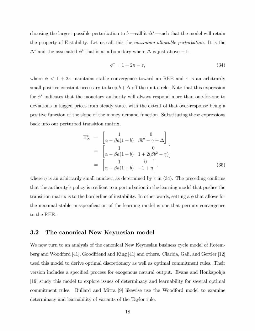
choosing the largest possible perturbation to b –call it ∆∗–such that the model will retain

the property of E-stability. Let us call this the maximum allowable perturbation. It is the

∆∗ and the associated φ∗ that is at a boundary where ∆ is just above −1:

φ∗ = 1 + 2κ− ε, (34)

where φ < 1 + 2κ maintains stable convergence toward an REE and ε is an arbitrarily

small positive constant necessary to keep b+∆ off the unit circle. Note that this expression

for φ∗ indicates that the monetary authority will always respond more than one-for-one to

deviations in lagged prices from steady state, with the extent of that over-response being a

positive function of the slope of the money demand function. Substituting these expressions

back into our perturbed transition matrix,

Π∗∆ =

∙1 0

α− βa(1 + b) βb2 − γ +∆

¸=

∙1 0

α− βa(1 + b) 1 + 2(βb2 − γ)

¸=

∙1 0

α− βa(1 + b) −1 + η

¸, (35)

where η is an arbitrarily small number, as determined by ε in (34). The preceding confirms

that the authority’s policy is resilient to a perturbation in the learning model that pushes the

transition matrix is to the borderline of instability. In other words, setting a φ that allows for

the maximal stable misspecification of the learning model is one that permits convergence

to the REE.

3.2 The canonical New Keynesian model

We now turn to an analysis of the canonical New Keynesian business cycle model of Rotem-

berg andWoodford [41], Goodfriend and King [41] and others. Clarida, Gali, and Gertler [12]

used this model to derive optimal discretionary as well as optimal commitment rules. Their

version includes a specified process for exogenous natural output. Evans and Honkapohja

[19] study this model to explore issues of determinacy and learnability for several optimal

commitment rules. Bullard and Mitra [9] likewise use the Woodford model to examine

determinacy and learnability of variants of the Taylor rule.

18

The behavior of the private sector is described by two equations. The aggregate demand

(IS) equation is a log-linearized Euler equation derived from optimal consumer behavior,

xt = E∗t xt+1 − σ[rt −E∗t πt+1 − rnt ], (36)

and the aggregate supply (AS) equation–indeed, the price setting rule for monopolistically

competitive firms is,

πt = κxt + βE∗t πt+1, (37)

where x is the log deviation of output from potential output, π is inflation, r is a short-

term interest rate controlled by the central bank, and rn is the natural interest rate. For

the application of Bullard and Mitra’s [8] (BM) example, we assume that rnt is driven by a

first-order autoregressive process,

rnt = ρrrnt−1 + r,t, (38)

0 ≤ |ρr| < 1, and r,t ∼ iid(0, σ2r). This is essentially Woodford’s [49] version of this model,

which specifies that aggregate demand responds to the deviation of the real rate, rt−Etπt+1

from the natural rate, rnt .

We need to close the model with an interest-rate feedback rule. We study three types of

policy rules. In the first set of experiments described in Section 3.3, a central bank chooses

an interest rate setting in each period as a reaction to observed events, such as inflation and

the output gap, without explicitly attempting to improve some measure of welfare. Instead,

the policy authority is mindful of the effect its policy has on the prospect of the economy

reaching REE and designs its rule accordingly. Bullard and Mitra [8] study such rules for

their properties in promoting learnable equilibria and consider that effort as prior to one of

finding optimal policy rules consistent with REE. We take this analysis further by seeking

to find policy rules that maximize learnability of agents’ models when policy influences the

outcome.

The information protocols in these experiments is as follows. Economic agents and the

central bank have the same information: the data and the perceived law of motion. Agents

form expectations based on recursive (least squares) estimation of a reduced form. The data

are regenerated each period, subject to the authority having implemented its policy and

19

agents’ having made investment and consumption decisions based on their newly formed

expectations. Since the central bank uses an arbitrary simple rule, it need not know the

true structure of the economy, but, being aware of how individuals form their expectations,

it designs policy that ensures the learnability of the PLM.

We assume that agents mistakenly specify a vector-autoregressive model in the endoge-

nous and exogenous variables of the model. That means we assume the learning model to be

overparameterized in comparison with the model implied by the MSV solution. The scaling

factors used in W1 to scale the perturbations to the PLM are the standard errors of the

coefficients obtained from an initial run of a recursive least squares regression of such a VAR

with data being updated by the true model, given an arbitrary but determinate parameter-

ization of the policy rule being studied. As noted earlier, an alternative approach would be

to revise the scalings with each trial policy, given that the VAR would likely change with

each parameterization of policy. We leave this for a revision.

3.3 Simple interest rate feedback rules

This section describes two versions of the Taylor rule analyzed by Bullard and Mitra [8]. The

complete system comprises equations (36)-(39), and the exogenous variable, rnt . The policy

instrument is the nominal interest rate, rt. The first policy rule specifies that the interest

rate responds to lagged inflation and the lagged output gap. In their paper, BM study the

role of interest-rate inertia and so include a lagged interest rate term.

rt = φππt−1 + φxxt−1 + φrrt−1 (39)

McCallum has advocated such a lagged data rule because of its implementability, given that

contemporaneous real-time data are generally unavailable to policy makers.

Some research suggests that forward-looking rules perform well in theory (see, e.g., Evans

and Honkapohja [19]) as well as in actual economies, such as Germany, Japan, and the US

(see Clarida, Gali, and Gertler [11]). Accordingly, BM propose the rule

rt = φπE∗t πt+1 + φxE

∗t xt+1 + φrrt−1. (40)

The expectations operator E∗ has an asterisk to indicate that expectations need not be

20

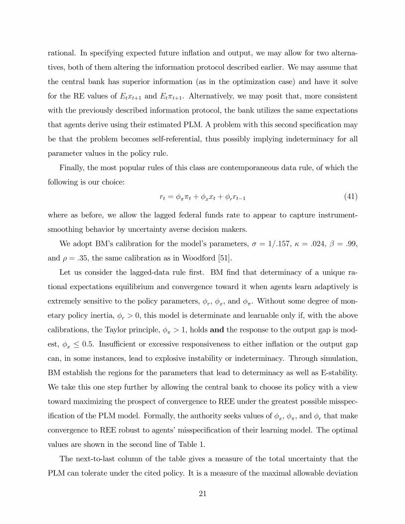
rational. In specifying expected future inflation and output, we may allow for two alterna-

tives, both of them altering the information protocol described earlier. We may assume that

the central bank has superior information (as in the optimization case) and have it solve

for the RE values of Etxt+1 and Etπt+1. Alternatively, we may posit that, more consistent

with the previously described information protocol, the bank utilizes the same expectations

that agents derive using their estimated PLM. A problem with this second specification may

be that the problem becomes self-referential, thus possibly implying indeterminacy for all

parameter values in the policy rule.

Finally, the most popular rules of this class are contemporaneous data rule, of which the

following is our choice:

rt = φππt + φxxt + φrrt−1 (41)

where as before, we allow the lagged federal funds rate to appear to capture instrument-

smoothing behavior by uncertainty averse decision makers.

We adopt BM’s calibration for the model’s parameters, σ = 1/.157, κ = .024, β = .99,

and ρ = .35, the same calibration as in Woodford [51].

Let us consider the lagged-data rule first. BM find that determinacy of a unique ra-

tional expectations equilibrium and convergence toward it when agents learn adaptively is

extremely sensitive to the policy parameters, φr, φx, and φπ. Without some degree of mon-

etary policy inertia, φr > 0, this model is determinate and learnable only if, with the above

calibrations, the Taylor principle, φπ > 1, holds and the response to the output gap is mod-

est, φx ≤ 0.5. Insufficient or excessive responsiveness to either inflation or the output gap

can, in some instances, lead to explosive instability or indeterminacy. Through simulation,

BM establish the regions for the parameters that lead to determinacy as well as E-stability.

We take this one step further by allowing the central bank to choose its policy with a view

toward maximizing the prospect of convergence to REE under the greatest possible misspec-

ification of the PLM model. Formally, the authority seeks values of φx, φπ, and φr that make

convergence to REE robust to agents’ misspecification of their learning model. The optimal

values are shown in the second line of Table 1.

The next-to-last column of the table gives a measure of the total uncertainty that the

PLM can tolerate under the cited policy. It is a measure of the maximal allowable deviation

21

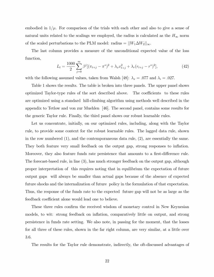
embodied in 1/µ. For comparison of the trials with each other and also to give a sense of

natural units related to the scalings we employed, the radius is calculated as the H∞ norm

of the scaled perturbations to the PLM model: radius = ||W1∆W2||∞.

The last column provides a measure of the unconditional expected value of the loss

function,

Lt =1000

2

∞Xj=0

βj[(πt+j − π∗)2 + λxx2t+j + λr(rt+j − r∗)2], (42)

with the following assumed values, taken from Walsh [48]: λx = .077 and λi = .027.

Table 1 shows the results. The table is broken into three panels. The upper panel shows

optimized Taylor-type rules of the sort described above. The coefficients to these rules

are optimized using a standard hill-climbing algorithm using methods well described in the

appendix to Tetlow and von zur Muehlen [46]. The second panel, contains some results for

the generic Taylor rule. Finally, the third panel shows our robust learnable rules.

Let us concentrate, initially, on our optimized rules, including, along with the Taylor

rule, to provide some context for the robust learnable rules. The lagged data rule, shown

in the row numbered (1), and the contemporaneous data rule, (2), are essentially the same.

They both feature very small feedback on the output gap, strong responses to inflation.

Moreover, they also feature funds rate persistence that amounts to a first-difference rule.

The forecast-based rule, in line (3), has much stronger feedback on the output gap, although

proper interpretation of this requires noting that in equilibrium the expectation of future

output gaps will always be smaller than actual gaps because of the absence of expected

future shocks and the internalization of future policy in the formulation of that expectation.

Thus, the response of the funds rate to the expected future gap will not be as large as the

feedback coefficient alone would lead one to believe.

These three rules confirm the received wisdom of monetary control in New Keynesian

models, to wit: strong feedback on inflation, comparatively little on output, and strong

persistence in funds rate setting. We also note, in passing for the moment, that the losses

for all three of these rules, shown in the far right column, are very similar, at a little over

3.6.

The results for the Taylor rule demonstrate, indirectly, the oft-discussed advantages of

22

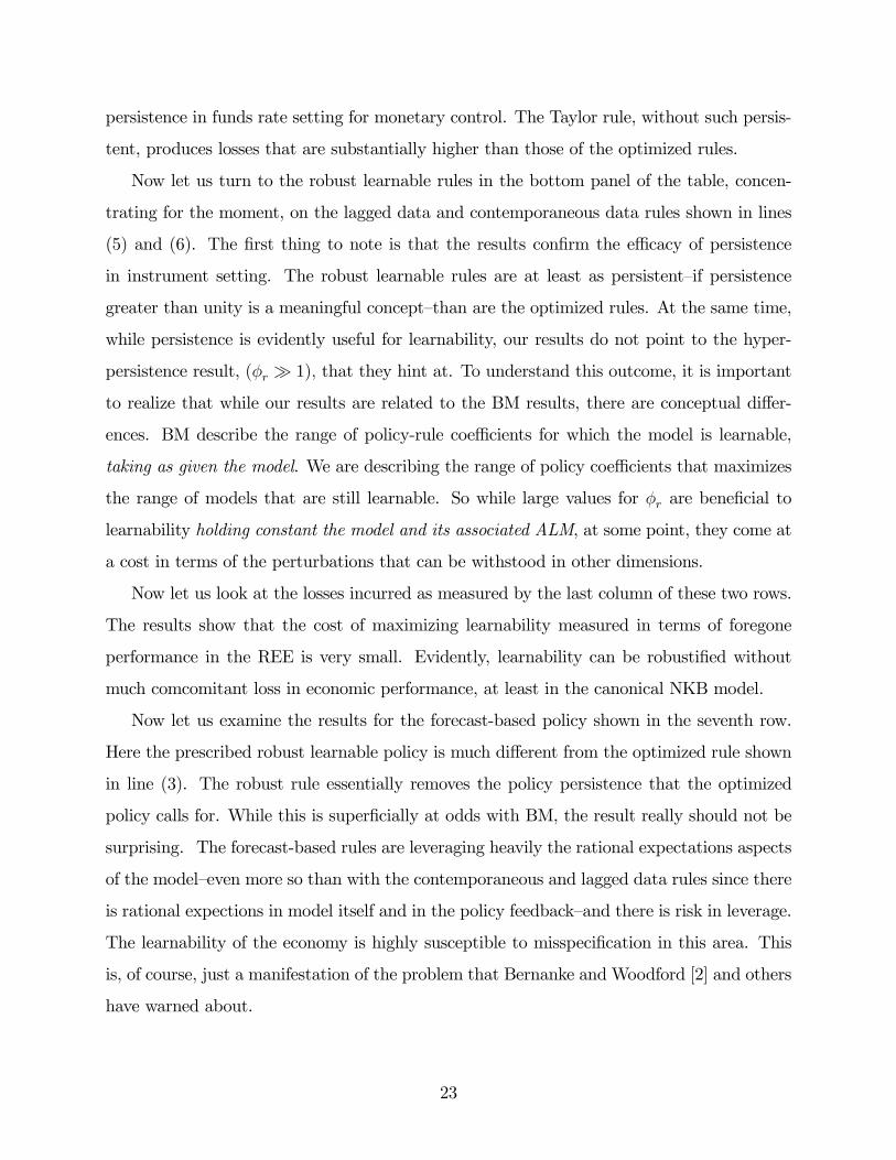
persistence in funds rate setting for monetary control. The Taylor rule, without such persis-

tent, produces losses that are substantially higher than those of the optimized rules.

Now let us turn to the robust learnable rules in the bottom panel of the table, concen-

trating for the moment, on the lagged data and contemporaneous data rules shown in lines

(5) and (6). The first thing to note is that the results confirm the efficacy of persistence

in instrument setting. The robust learnable rules are at least as persistent—if persistence

greater than unity is a meaningful concept—than are the optimized rules. At the same time,

while persistence is evidently useful for learnability, our results do not point to the hyper-

persistence result, (φr À 1), that they hint at. To understand this outcome, it is important

to realize that while our results are related to the BM results, there are conceptual differ-

ences. BM describe the range of policy-rule coefficients for which the model is learnable,

taking as given the model. We are describing the range of policy coefficients that maximizes

the range of models that are still learnable. So while large values for φr are beneficial to

learnability holding constant the model and its associated ALM, at some point, they come at

a cost in terms of the perturbations that can be withstood in other dimensions.

Now let us look at the losses incurred as measured by the last column of these two rows.

The results show that the cost of maximizing learnability measured in terms of foregone

performance in the REE is very small. Evidently, learnability can be robustified without

much comcomitant loss in economic performance, at least in the canonical NKB model.

Now let us examine the results for the forecast-based policy shown in the seventh row.

Here the prescribed robust learnable policy is much different from the optimized rule shown

in line (3). The robust rule essentially removes the policy persistence that the optimized

policy calls for. While this is superficially at odds with BM, the result really should not be

surprising. The forecast-based rules are leveraging heavily the rational expectations aspects

of the model—even more so than with the contemporaneous and lagged data rules since there

is rational expections in model itself and in the policy feedback—and there is risk in leverage.

The learnability of the economy is highly susceptible to misspecification in this area. This

is, of course, just a manifestation of the problem that Bernanke and Woodford [2] and others

have warned about.

23

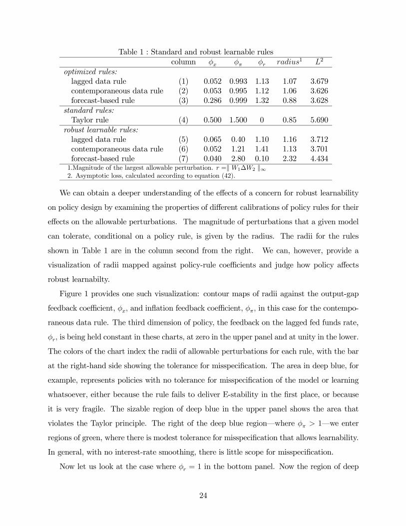
Table 1 : Standard and robust learnable rulescolumn φx φπ φr radius1 L2

optimized rules:lagged data rule (1) 0.052 0.993 1.13 1.07 3.679contemporaneous data rule (2) 0.053 0.995 1.12 1.06 3.626forecast-based rule (3) 0.286 0.999 1.32 0.88 3.628

standard rules:Taylor rule (4) 0.500 1.500 0 0.85 5.690

robust learnable rules:lagged data rule (5) 0.065 0.40 1.10 1.16 3.712contemporaneous data rule (6) 0.052 1.21 1.41 1.13 3.701forecast-based rule (7) 0.040 2.80 0.10 2.32 4.4341.Magnitude of the largest allowable perturbation. r =kW1∆W2 k∞2. Asymptotic loss, calculated according to equation (42).

We can obtain a deeper understanding of the effects of a concern for robust learnability

on policy design by examining the properties of different calibrations of policy rules for their

effects on the allowable perturbations. The magnitude of perturbations that a given model

can tolerate, conditional on a policy rule, is given by the radius. The radii for the rules

shown in Table 1 are in the column second from the right. We can, however, provide a

visualization of radii mapped against policy-rule coefficients and judge how policy affects

robust learnabilty.

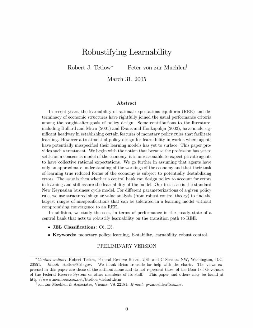
Figure 1 provides one such visualization: contour maps of radii against the output-gap

feedback coefficient, φx, and inflation feedback coefficient, φπ, in this case for the contempo-

raneous data rule. The third dimension of policy, the feedback on the lagged fed funds rate,

φr, is being held constant in these charts, at zero in the upper panel and at unity in the lower.

The colors of the chart index the radii of allowable perturbations for each rule, with the bar

at the right-hand side showing the tolerance for misspecification. The area in deep blue, for

example, represents policies with no tolerance for misspecification of the model or learning

whatsoever, either because the rule fails to deliver E-stability in the first place, or because

it is very fragile. The sizable region of deep blue in the upper panel shows the area that

violates the Taylor principle. The right of the deep blue region–where φπ > 1–we enter

regions of green, where there is modest tolerance for misspecification that allows learnability.

In general, with no interest-rate smoothing, there is little scope for misspecification.

Now let us look at the case where φr = 1 in the bottom panel. Now the region of deep

24

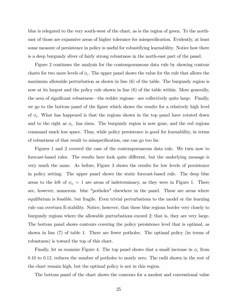
blue is relegated to the very south-west of the chart, as is the region of green. To the north-

east of those are expansive areas of higher tolerance for misspecification. Evidently, at least

some measure of persistence in policy is useful for robustifying learnability. Notice how there

is a deep burgundy sliver of fairly strong robustness in the north-east part of the panel.

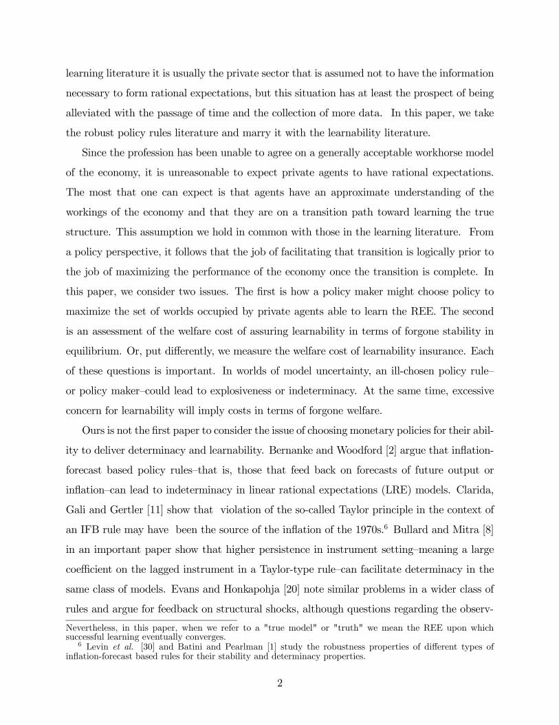
Figure 2 continues the analysis for the contemporaneous data rule by showing contour

charts for two more levels of φr. The upper panel shows the value for the rule that allows the

maximum allowable perturbation as shown in line (6) of the table. The burgundy region is

now at its largest and the policy rule shown in line (6) of the table within. More generally,

the area of significant robustness–the redder regions–are collectively quite large. Finally,

we go to the bottom panel of the figure which shows the results for a relatively high level

of φr. What has happened is that the regions shown in the top panel have rotated down

and to the right as φr has risen. The burgundy region is now gone, and the red regions

command much less space. Thus, while policy persistence is good for learnability, in terms

of robustness of that result to misspecification, one can go too far.

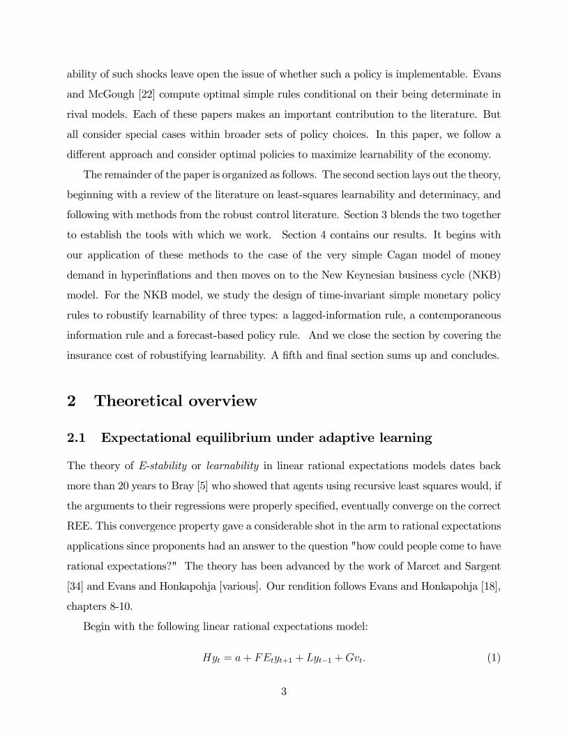
Figures 1 and 2 covered the case of the contemporaneous data rule. We turn now to

forecast-based rules. The results here look quite different, but the underlying message is

very much the same. As before, Figure 3 shows the results for low levels of persistence

in policy setting. The upper panel shows the static forecast-based rule. The deep blue

areas to the left of φπ = 1 are areas of indeterminacy, as they were in Figure 1. There

are, however, numerous blue "potholes" elsewhere in the panel. These are areas where

equilibrium is feasible, but fragile. Even trivial perturbations to the model or the learning

rule can overturn E-stability. Notice, however, that these blue regions border very closely to

burgundy regions where the allowable purturbations exceed 2; that is, they are very large.

The bottom panel shows contours covering the policy persistence level that is optimal, as

shown in line (7) of table 1. There are fewer potholes. The optimal policy (in terms of

robustness) is toward the top of this chart.

Finally, let us examine Figure 4. The top panel shows that a small increase in φr from

0.10 to 0.12, reduces the number of potholes to nearly zero. The radii shown in the rest of

the chart remain high, but the optimal policy is not in this region.

The bottom panel of the chart shows the contours for a modest and conventional value

25

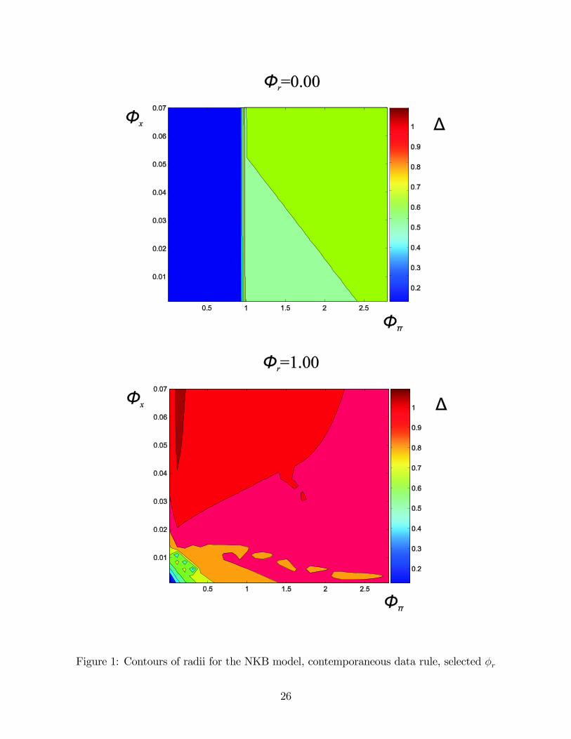
Figure 1: Contours of radii for the NKB model, contemporaneous data rule, selected φr

26

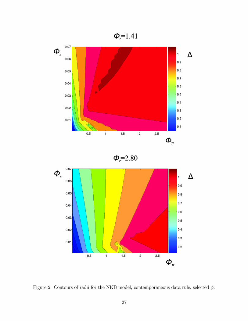
Figure 2: Contours of radii for the NKB model, contemporaneous data rule, selected φr

27

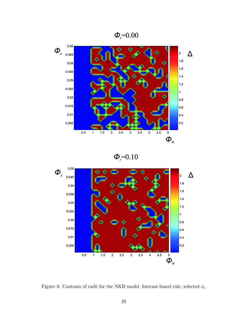
Figure 3: Contours of radii for the NKB model, forecast-based rule, selected φr

28

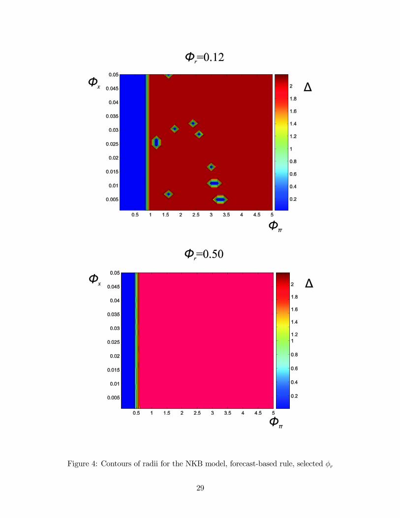
Figure 4: Contours of radii for the NKB model, forecast-based rule, selected φr

29

of funds rate persistence, φr = 0.50. The potholes have now completely disappeared, but

the large red region is less robust than the burgundy regions in the previous charts. Not

shown in these charts are still higher levels of persistence. These involve still lower levels of

robustness, with radii for φr > 1 associated with radii that are less than half the magnitude

of the maximum allowable perturbation for this rule. Higher levels of persistence in policy

setting are deleterious for robustification of model learnabilty.24

Of course these particular results are contingent on the relative weightings for perturba-

tions, captured in W1, and our selection is just one of many that could have been made. For

the numerical experiments, the weightings were set equal to the standard deviations of the

coefficients of a first-order VAR for the output gap, inflation, the interest rate, and the nat-

ural rate, estimated at the beginning of each experiment via recursive least squares. These

should give a rough idea of the relative uncertainties associated with the coefficients of the

PLM. Whether using estimated standard deviations to scale the relative impact of Knight-

ian model uncertainty on the elements of the PLM is proper or desirable can be debated,

of course. Further, since in a recursive world, the data are generated by the actual law of

motion, which depends on the current setting of policy parameters and expectations based

on the estimated PLM, the coefficients of the VAR model are not invariant to policy. Such

issues we take up in a revision, when we will also deploy relative scalings obtained from a

VAR that is re-estimated with each trial vector of policy parameters during the grid search.

For now the salient point is that robustness of learning in the presence of model uncertainty

is not the same thing as choosing the rule parameters for which the E-stable region of a

given model is largest.

4 Concluding remarks

We have argued that model uncertainty is a serious issue in the design of monetary policy.

On this score we are in good company. Many authors have advanced that minimizing a

loss function subject to a given model presumed to be known with certainty is no longer

24 We tested φr up to nearly 20. What we found is that the radii fell as φr rose for intermediate levels,and then rose slowly again for φr À 1. However, for no level of φr could we find radii that came anywhereclose to the maximum allowable perturbation shown in row (7) of the table.

30

best practice for monetary authorities. Central bankers must also take model uncertainty

and learning into account. Where this paper differs from its predecessors is that we unify

three considerations: uncertainty about the model, the learning mechanism used by private

agents, and steps the monetary authority can take to address these issues. In particular,

we examine a central bank that designs monetary policy to maximize the possible worlds in

which ill-informed private agents need time to learn about their particular world and still

allow convergence toward the rational expectations equilibrium (REE) of the true economy.

The motivation for this approach is straightforward: if economics as a profession cannot

agree on what the true model of the economy is, it is a leap of faith to expect private agents

to agree, coordinate, and find the REE themselves. Policy makers should do their part to

facilitate the process of learning the REE through the design of policy, where the task of

assuring convergence on REE is logically prior to the question of the design of policy, once

that convergence has been achieved.

This paper has married the literature on adaptive learning to that of structured robust

control to examine what policy makers can do to facilitate learning. We have introduced

some tools with which the questions that Bullard and Mitra [8] are asking can be broadened

and generalized.

31

References

[1] Batini, N. and Pearlman, J. (2002) "Too much too soon: instability and indeterminacy

with forward-looking rules" unpublished manuscript, Bank of England.

[2] Bernanke, B. andWoodford, M.(1997) "Inflation forecasts andmonetary policy" Journal

of Money, Credit and Banking 24: 653-684.

[3] Blanchard, O. and Khan, C. (1980) "The solution of linear difference equations under

rational expectations" Econometrica,48: 1305-1311.

[4] Brainard, W. (1967) "Uncertainty and the effectiveness of monetary policy" American

Economic Review 57(2): 411-425.

[5] Bray, M. (1982) "Learning, estimation and the stability of rational expectations equi-

libria" Journal of Economic Theory,26: 318-339.

[6] Bray, M. and Savin, N. (1986) "Rational expectations equilibria, learning and model

specification" Econometrica,54: 1129-1160.

[7] Bullard, J. and Eusepi, S. (2003) "Did the great inflation occur despite policymaker

commitment to a Taylor rule?" Federal Reserve Bank of St. Louis working paper no.

2003-13.

[8] Bullard, J. and Mitra, K. (2003) "Determinacy, learnability and monetary policy iner-

tia" Federal Reserve Bank of St. Louis working paper 2000-030A (revised version: March

2003)

[9] Bullard, J. and Mitra, K. (2002), "Learning about monetary policy rules", Journal of

Monetary Economics,49: 1105-1139.

[10] Cagan, P (1956) "The monetary dynamics of hyperinflations" in M. Friedman (ed.)

Studies in the Quantity Theory of Money (Chicago: University of Chicago Press).

[11] Clarida, Richard, Jordi Gali, and Mark Gertler (1998) "Monetary Policy Rules in Prac-

tice: Some International Evidence" European Economic Review,42: 1033-1067.

32

[12] Clarida, Richard, Jordi Gali, and Mark Gertler (1999) "The Science of Monetary Policy:

A New Keynesian Perspective" Journal of Economic Literature,70: 807-824.

[13] Coenen, G. (2003) "Inflation persistence and robust monetary policy design" European

Central Bank working paper no. 290 (November).

[14] Dahleh, M and Diaz-Bobillo, I. (1995) Control of Uncertain Systems: A Linear Pro-

gramming Approach (Englewood Hills, NJ: Prentice Hall).

[15] Delong, B. (1997) "America’s peacetime inflation: the 1970s" in C. Romer and D. Romer

(eds.) Reducing Inflation: motivation and strategies (Chicago: University of Chicago

Press): 247-276.

[16] Doyle, J. "Analysis of feedback systems with structured uncertainties" IEEE Proceed-

ings,133 (part D, no. 2): 45-56.

[17] Ehrmann, M. and Smets, F. (2003) "Uncertain potential output: implications for mon-

etary policy" Journal of Economic Dynamics and Control,27: 1611-1638.-

[18] Evans, G. and Honkapohja, S. (2001) Learning and Expectations in Macroeconomics

(Princeton: Princeton University Press).

[19] Evans, G.W. and Honkapohja, S.(2002) "Monetary Policy, Expectations, and Com-

mitment" unpublished manuscript, University of Oregon and Oregon State University

(May).

[20] Evans, G. and Honkapohja, S. (2003) "Expectations and the stability for optimal mon-

etary policies" Review of Economic Studies,70: 807-824.

[21] Evans, G. and McGough, B. (2003) "Stable sunspot solutions in models with prede-

termined variables" unpublished manuscript, University of Oregon and Oregon State

University (May).

[22] Evans, G. and McGough, B. (2004) "Optimal constrained monetary policy rules" un-

published paper presented to the Society for Computational Economics conference, July

8-10, 2004, University of Amsterdam, Amsterdam.

33

[23] Garratt, A. and Hall, S.(1997) "E-equilibria and adaptive expectations: output and

inflation in the LBS model" Journal of Economic Dynamics and Control,21: 87-96.

[24] Giordani, P. and Soderlind, P. (2004) "Solution of macromodels with Hansen-Sargent

robust policies: some extensions" Journal of Economic Dynamics & Control,28: 2367-

2397.

[25] Giannoni, M.P. (2002) "Does model uncertainty justify caution?: model uncertainty in

a forward-looking model" Macroeconomic Dynamics,6(1): 111-144.

[26] Goodfriend, M. and King, R. (1997) "The new neo-classical synthesis and the role of

monetary policy"

[27] Hansen, L and Sargent, T. (2003) Misspecification in Recursive Macroeconomic Theory

(unpublished monograph, November 2003)

[28] Hansen, L.P. and Sargent, T.J. (2003) "Robust control of forward-looking models"

Journal of Monetary Economics 50(3): 581-604.

[29] Levin, A.T., Wieland, V. andWilliams, J.C. (1999) "Monetary policy rules under model

uncertainty" in J.B. Taylor (ed.)Monetary Policy Rules (Chicago: University of Chicago

Press).

[30] Levin, A.T., Wieland, V. and Williams, J.C. (1999) "The performance of forecast-based

monetary policy rules under model uncertianty"American Economic Review,93(2): 622-

645.

[31] Lubik, T.A. and Schorfheide, F. (2003) "Computing sunspot equilibria in linear rational

expectations models" Journal of Economic Dynamics and Control,28(2): 273-285.

[32] Lubik, T.A. and Schorfheide, F. (2004) "Testing for indeterminacy: an application to

U.S. monetary policy" American Economic Review,94(1): 190-217.

[33] Marcet, A and Nicolini, J.P. (2003) "Recurrent hyperinflations and learning" American

Economic Review,96:1476-1498.

34

[34] Marcet, A. and Sargent, T .J.(1989) "Convergence of least squares learning mechanisms

in self-referential linear stochastic models" Journal of Economic Theory,48(2): 337-368

[35] McCallum, B. (1983) "On non-uniqueness in rational expectations models: an attempt

at perspective" Journal of Monetary Economics,11: 134:168.

[36] Onatski, A (2003) "Robust monetary policy under model uncertainty: incorporating

rational expectations" unpublished manuscript, Columbia University.

[37] Onatski, A. and Stock, J. (2002) "Robust monetary policy under model uncertainty in

a small model of the U.S. economy" Macroeconomic Dynamics

[38] Onatski, A and N. Williams (2003) "Modeling model uncertainty" Journal of the Eu-

ropean Economic Association,1: 1087-1122.

[39] Orphinides, A., Porter, R., Reifschneider, D., Tetlow, R., and Finan, F. (2000) "Errors

in the measurement of the output gap and the design of monetary policy" Journal of

Economics and Business,52(1/2): 117-141.

[40] Rogoff, A. (1985) "The optimal degree of commitment to an intermediate monetary

target" 100,Quarterly Journal of Economics,4 (November): 1169-1190.

[41] Rotemberg, J. and Woodford, M. (1997) "An optimization-based econometric frame-

work for the evaluation of monetary policy" in B. Bernanke and J. Rotemberg (eds.)

NBER Macroeconomics Annual (Cambridge, MA: MIT Press): 297-345.

[42] Sack, B. (1999) "Does the fed act gradually: a VAR analysis" Journal of Monetary

Economics,46(1): 229-256.

[43] Sargent, T. (1999) "Comment" in J.B. Taylor (ed.) Monetary Policy Rules (Chicago:

University of Chicago Press): 144-154

[44] Soderstrom, U. (2002) "Monetary policy with uncertain parameters" Scandinavian

Journal of Economics,104(1): 125-145.

[45] Taylor, J.B.(1993) "Discretion versus policy rules in practice" Carnegie-Rochester Con-

ference Series on Public Policy,39: 195-214.

35

[46] Tetlow. R. and von zur Muehlen, P. (2001) "Robust monetary policy with misspecified

models: does model uncertainty always call for attenuated policy?" Journal of Economic

Dynamics and Control 25(6/7): 911-949.

[47] Tetlow, R. and von zur Muehlen, P. (2004) "Avoiding Nash Inflation: Bayesian and

robust responses to model uncertainty" 7,Review of Economic Dynamics, 4 (October):

869-899.

[48] Walsh, C. E (2004) "Parametric misspecification and robust monetary policy rules,"

unpublished manuscript, University of California, Santa Cruz.

[49] Woodford, M.(1998) "Optimal Monetary Policy Inertia" Mimeo. Prineton University,

December 14.

[50] Woodford, M.(2003) "Optimal Interest Rate Smoothing" Review of Economic Studies

70: 861-886.

[51] Woodford, M. (2003) Interest and Prices: Foundations of a theory of monetary policy

(Princeton: Princeton University Press).

[52] Zames, G. (1966) "On the input-output stability of nonlinear time-varying feedback

systems, parts I and II" IEEE Transactions on Automatic Control,AC-11: 228, 465.

[53] Zhou, K., Doyle,J.C., and Glover, K. (1996) Robust and Optimal Control (Englewood

Cliffs, NJ.: Prentice-Hall).

[54] Zhou, K., with Doyle,J.C. (1998) Essentials of Robust Control (Englewood Cliffs, NJ.:

Prentice-Hall).

36

5 Appendix

Implementation of the techniques outlined in Section 2.2 requires some familiarity with

Matlab’s µ-Analysis and Synthesis Toolbox. Matlab’s User’s Guide and Zhou and Doyle’s

Essentials of Robust Control go a long way to aid the prospective user. The reader should be

forewarned, however, that this technique and its literature have been developed in large part

by aero-space engineers whose technical jargon is as peculiar and insular as any economist

might dream of. From an economist’s perspective, the examples in the User’s Guide range

from the exotic (design of F-14 fighter jets) to incomprehensible.

For illustrative purposes, let the perturbed system be one involving two state variables,

and let the dynamic model be represented by A, where

A =

∙a11 a12a21 a22

¸Let us further assume that elements a12 and a21 are subject to scaled structured perturbations

assumed to be scalar for our purposes:

AP =

∙a11 a12 + σ1∆12

a21 + σ2∆21 a22

¸The σs give relative scalings to the perturbations andmight be reasonably related to known or

estimated stanstard deviations of the elements in A. While calculations of µ are unaffected if

all scaling factors are multiplied by the same factor, µ and its inverse, the maximal allowable

range of perturbation, will be affected by the relative scalings imposed on ∆. So, it is of

some consequence to give some thought to scaling. The perturbed system can be represented

as the following product of matrices,

AP = A+W1∆W2,

where

∆ =

∙∆12 00 ∆21

¸W1 =

∙σ1 00 σ2

¸W2 =

∙0 11 0

¸,

where σ1 and σ2 are scalar weights. To continue, we need to generate the frequency response,

G2 in (21)-(22). First create the "system"

G =

∙A | W2

W1 | 0k,k

¸using the Matlab command

37

G = pck(A,W1,W2,zeros(k, k));

where k is the number of diagonal elements in ∆. Next, create the frequency response over

a range of frequencies, say 20 points on ω ∈ [0, 2π]

ω =linspace(0,2*pi,20);

and calculate

G2(ω) = W2(e−iω −A)−1W1

with

G2= frsp(G,ω,1);

As shown in section 2.2, for a given specification of the policy rule, we seek the largest

structured singular value of G2 over the frequency range, ω. The Matlab call

opt = [’s’,’w’]; [bnds,rowd,sens,rowp,rowg]=mu(G2,blk,opt);

where specifying "opt" as above eliminates annoying output messages. The matrix, bnds,

contains the upper and lower bounds of µ. For reasons that are explained in Zhou and Doyle

[54], blk is a k × 2 input matrix that must be specified by the user. If the perturbations are

assumed to be scalar in nature, representing one-time jumps, for example, blk has negative

’one’s in the first column and zeros or ’one’s in column two. In the above case, blk=∙−1 0−1 0

¸.

The relevant numbers are the lower bounds of µ, contained in the second column of bnds. For

real, scalar perturbations, i.e., those not involving the complex domain, Matlab has trouble

computing lower bounds on µ. The result is an annoying stream of Matlab warnings. To

get around this, one can tweak the system slightly to introduce a second very small pertur-

bation matrix of complex perturbations too small to affect the results, using the following

commands:

alpha = .1;

fix = [eye(kblk);alpha*eye(kblk)];

blkr = [blk;abs(blk)];

G2r = mmult(fix,G2,fix’);

opt = [’s’,’w’]; [bnds,rowd,sens,rowp,rowg]=mu(G2r,blkr,opt);

38

The perturbation matrices over the frequencies, ω can be retrieved with the command

Delta=unwrapp(pvec,blk);

Lower bounds on µ are stored in the second column of bnds. The value of interest is the

maximum in that column. At the frequency, for which µ is the maximum, the norm of ∆ is

the inverse of µ. This is the maximal allowable range of perturbations. The policy maker

chooses parameters in the interest rate reaction function that cause this range to be the

largest.

39