IEEE INTELLIGENT TRANSPORTATION SYSTEMS MAGAZINE 1

Robust Vehicular Navigation and Map-Matchingin Urban Environments with IMU, GNSS,

and Cellular SignalsZaher M. Kassas,Senior Member, IEEE, Mahdi Maaref, Joshua Morales,Student Member, IEEE,

Joe Khalife,Student Member, IEEE, and Kimia Shamaei,Student Member, IEEE,

Abstract—A framework for ground vehicle navigation that usescellular signals of opportunity (SOPs), a digital map, an inertialmeasurement unit (IMU), and a global navigation satellite system(GNSS) receiver is developed. This framework aims to enablenavigation in urban environment where GNSS signals could beunusable or unreliable. The proposed framework employs anextended Kalman filter (EKF) to fuse pseudorange observablesextracted from cellular SOPs, IMU measurements, and GNSS-derived position estimates (when available). The EKF is coupledwith a closed-loop map-matching approach. The frameworkassumes the positions of the cellular towers to be known andit estimates the vehicle’s states (position, velocity, orientation,and IMU biases) along with the difference between the vehicle-mounted receiver clock error states (bias and drift) and eachcellular SOP clock error states. Experimental results withcellularlong-term evolution (LTE) SOPs are presented, evaluating theefficacy and accuracy of the proposed framework in a deepurban area with a limited sky view. The experimental resultsdemonstrate a position root-mean squared error (RMSE) of 2.8 mover a 1380 m trajectory during which GNSS signals are availableand an RMSE of 3.12 m over the same trajectory during whichGNSS signals were unavailable for 330 m. Moreover, comparedtonavigation with a traditional GNSS-IMU integrated systems, it isdemonstrated that the proposed framework reduces the positionRMSE by 22% whenever GNSS signals are available and by 81%whenever GNSS signals are unavailable.

I. I NTRODUCTION

Accurate anytime, anywhere navigation has become anessential requirement in our modern life, especially with theadvent of self-driving cars. Over the years, various toolswere developed to meet this stringent requirement. At thecore, traditional vehicular navigation systems couple globalnavigation satellite system (GNSS) with on-board sensors,such as an inertial measurement unit (IMU). Moreover, suchnavigation systems may have access to digital maps fromwhich positioning information may be extracted. In a nutshell,GNSS receivers are used to aid the on-board IMU and toprovide a navigation solution in a global frame, which getsmatched to a point in the digital map by means of map-matching techniques [1]–[3].

While IMU sensors provide an accurate short-term naviga-tion solution, one cannot rely on them as a standalone, accuratesolution for long-term navigation. This is due to the fact thatthe noisy outputs of IMUs are integrated through an inertialnavigation system (INS), causing pose estimation errors to

This work was supported in part by the Office of Naval Research(ONR)under Grant N00014-16-1-2305 and Grant N00014-16-1-2809 and in part bythe National Science Foundation (NSF) under Grant 1751205.

accumulate over time [4], [5]. The accumulated error isdependent on the quality of the IMU and compromises the safeand efficient operation requirements in urban navigation. Thus,in long-term driving, an IMU sensor may become unreliableand an aiding source is needed to correct the drift and improvethe navigation solution. Therefore, the navigation systems on-board ground vehicle’s today typically include other sensors(e.g., camera, laser, and sonar) to aid the vehicle’s IMU.However, such aiding sensors may violate cost, size, weight,and power (C-SWAP) constraints. A common approach tocorrect for the drift in the IMU’s navigation solution is tofuse IMU data and GNSS signals. While GNSS provides anaccurate position estimate with respect to a global frame, itssignals are severely attenuated in deep urban canyons, makingthem unreliable to aid the IMU’s navigation solution.

Recently, signals of opportunity (SOPs) have been usedto overcome GNSS drawbacks. SOPs are ambient radio-frequency signals that can be exploited for navigation pur-poses, such as digital television, cellular signals [6]–[9], andAM/FM radio signals [10], [11]. Such signals are abundantin urban canyons and are free to use. Among SOPs, cellularsignals are particularly attractive for navigation and offerseveral advantages for positioning, namely [12], [13]:

• Availability: cellular base transceiver stations (BTSs) areabundant in order to service the billions of smart phoneand tablet devices with wireless capabilities. Moreover,cellular signals are available in several bands, aggregatingto tens of megahertz of usable cellular radio frequencyspectrum, making them robust against jamming andspoofing attacks or service outage in certain bands orproviders.

• Geometric diversity: the cellular system configuration,by construction, yields low horizontal dilution of preci-sion (HDOP); hence they offer a favorable BTS geometryfor positioning, unlike certain terrestrial SOPs which tendto be co-located (e.g., digital television).

• Large bandwidth: cellular signals can have a bandwidthup to 20 MHz, which yields precise time-of-arrival (TOA)estimates and in turn precise positioning.

• High received power: the received carrier-to-noise ratiofrom nearby cellular BTSs is commonly tens of dBshigher when compared to GNSS satellite vehicle (SV)signals, which makes cellular signals more reliable insome instances for TOA estimation.

IEEE INTELLIGENT TRANSPORTATION SYSTEMS MAGAZINE 2

This article presents a robust vehicular navigation frame-work for navigating in both GNSS-available and GNSS-deniedurban environments. A computationally efficient extendedKalman filter (EKF) that fuses digital map data, IMU data,GNSS-derived estimated position, and cellular SOP pseudo-ranges is adopted. When GNSS signals are unavailable orcompromised, the framework extracts navigation observablesfrom cellular signals and fuses them with IMU and map dataand continuously estimates the vehicle’s states for subsequenttime as it navigates without GNSS signals. When GNSSsignals are available, the navigation solution is obtainedbyfusing the IMU data, map data, cellular signals, and GNSS-based estimations. In both modes, a closed-loop map-matchingapproach is developed, where the refined vehicle positionestimate obtained from fusing cellular SOP pseudorange, IMU,GNSS-based estimations (if GNSS is available), and digitalroad maps is used in a feedback to correct estimates of theclock error states.

Fig. 1 illustrates the proposed map-matching approach.Fig. 1(a) illustrates a high-level diagram of the cellular-aidedIMU framework. Fig. 1(b) demonstrates the proposed closed-loop map-matching approach with inputs being GNSS signals,cellular SOP signals, IMU data, and digital road networkand the output being the refined navigation solution. As canbe seen, the algorithm is closed-loop where the navigationsolution is fed back to correct estimates of the receiver andcellular SOPs clock error states.

Map-matching

Navigationsolution

Receiver & cellular SOPs'clock error estimates

signals

IMU

GNSS signals(if available)

(a)

(b)

IMURadio

front-end

Inertialnavigationsystem

Receiver andcellular clock

error

predictionEKF

EKFupdate

Receivers

GPS

Cellular

IMU data

.

.

.

.

.

.

Sampled signals

Loosely-coupled

map-matching

.

.

.

extended Kalman filter

Cellular

navigationsolution

Vehicle'sDigital map

Fig. 1. (a) A high-level diagram of the cellular-aided IMU frameworkwhere an IMU sensor is used in a loosely-coupled fashion. (b)The proposedclosed-loop map-matching approach. The algorithm is closed-loop where thenavigation solution is fed back to correct estimates of the receiver and cellularSOPs clock error states.

To evaluate the performance of the proposed ground vehiclenavigation algorithm, two experimental tests were performed

using ambient cellular long-term evolution (LTE) SOPs in (1)an urban environment where signal attenuation severely affectsthe received pseudoranges and (2) an environment whereSOPs have poor geometric diversity. Experimental resultswith the proposed method are presented illustrating closematch between the vehicle’s true trajectory and that estimatedusing the cellular-aided IMU + map data, particularly inthe GNSS-denied environments with a limited line-of-sight(LOS) to the open sky. The experimental results demonstratea position root-mean squared error (RMSE) of 2.8 m over a1380 m trajectory with available GNSS signals and RMSEof 3.12 m with partially unavailable GNSS signals. Moreover,it is demonstrated that incorporating the proposed algorithmimproves the position RMSE by 22% and 81%, in GNSS-available and GNSS-denied environments, respectively, fromthe RMSE obtained by a GNSS-IMU navigation solution.

The remainder of this article is organized as follows. SectionII describes the dynamics models for the IMU and SOPs aswell as the model for the digital map. Section III proposes anEKF-based framework for fusing IMU, GNSS-based estima-tions, digital map and cellular pseudoranges in both GNSS-available and GNSS-denied environments. Section IV providesthe experimental results and the performance analysis of theproposed framework in deep urban environment with a limitedLOS to the open sky. Concluding remarks are given in SectionV.

II. NAVIGATION FRAMEWORK MODEL DESCRIPTION

This section describes the models of the different compo-nents of the vehicular navigation framework: IMU, cellularSOP, GNSS receiver, and digital map.

A. IMU Measurement Model

An IMU produces measurements of angular rate and spe-cific force. In order to use these measurements, the IMU’sorientation, position, velocity, and measurement biases mustbe estimated. In this work, an IMU state vectorxv consistingof 16 states is used and is given by

xv =[

IGq

T , pT

v , pT

v , bTg , bTa

]T

, (1)

where IGq is a four-dimensional (4-D) unit quaternion rep-

resenting the IMU’s orientation (i.e., rotation from a globalframeG to the IMU’s body frameI); pv , [pv,x, pv,y, pv,z]

T

and pr are the three-dimensional (3-D) position and velocityof the vehicle, respectively, expressed inG; andbg andba arethe 3-D gyroscope and accelerometer biases, respectively.

The IMU’s measurements of the angular rateω and specificforcea are available everyT seconds and can be modeled as

ω = Iω + bg + ng, (2)

a = R[IkG q](

GaI −Gg

)

+ ba + na, (3)

respectively, whereIω is the IMU’s true rotation rate;ng

is a measurement noise vector, which is modeled as a whitenoise sequence with covarianceQg; R[IkG q] is the equivalentrotation matrix of IkG q; GaI is the IMU’s true acceleration

IEEE INTELLIGENT TRANSPORTATION SYSTEMS MAGAZINE 3

in frame G; and na is a measurement noise vector, whichis modeled as a white noise sequence with covarianceQa.The evolution of the gyroscope and accelerometer biases aremodeled as random walks, i.e.,ba = wa andbg = wg, wherewa andwg are modeled as zero-mean random vectors withcovariancesσ2

waI3×3 andσ2

wgI3×3, respectively, whereIn×n

denotes ann×n identity matrix. The equivalent rotation matrixR[q] of the quaternion vectorq = [q0, qv1 , qv2 , qv3 ]

T is

R[q] = [r1, r2, r3] , r1 =

q20 + q2v1 − q2v2 − q2v32(qv1qv2 − q0qv3)2(qv1qv3 + q0qv2)

,

r2 =

2(qv1qv2 + q0qv3)q20 − q2v1 + q2v2 − q2v32(qv2qv3 − q0qv1)

,

r3 =

2(qv1qv3 − q0qv3)2(qv2qv3 + q0qv1)

q20 − q2v1 − q2v2 + q2v3

.

The measurements in (2)-(3) will be used in the EKFto perform a time update of the estimate ofxv betweenmeasurement updates. This will be discussed in SubsectionIII-A.

B. GNSS Received Signal Model

A GNSS receiver estimates the receiver’s states, namelythe 3-D positionpv and clock biasδtr, from pseudorangeobservables made on GNSS satellites. A simplified model ofthe pseudorange made by the receiver on them-th GNSSsatellite at time-stepk, which represents discrete time attk = kT + t0 for an initial time t0 and sampling timeT ,is given by

zGNSS,m(k) =∥

∥pv(k)− pGNSS,m(k′m)∥

∥

2

+ c · [δtr(k)− δtGNSS,m(k′m)]

+ cδtiono,GNSS,m(k) + cδttropo,GNSS,m(k)

+ vGNSS,m(k),

k =1, 2, . . . , m = 1, . . . ,MGNSS,

whereMGNSS is the total number of available GNSS satellites;k′m represents discrete time attk′

m= kT +t0−δtTOFm

whereδtTOFm

is the true time-of-flight of the signal from them-thGNSS satellite to the receiver;c is the speed-of-light;pGNSS,m

andδtGNSS,m are the 3-D position vector and the clock biasof the m-th GNSS satellite, respectively;δtiono,GNSS,m andδttropo,GNSS,m are the ionospheric and tropospheric delaysfrom the m-th GNSS satellite to the receiver, respectively;andvGNSS,m is the measurement noise, which is modeled asa zero-mean white Gaussian random sequence with varianceσ2

GNSS,m

C. Cellular SOP Received Signal Model

Cellular towers transmit signals for synchronization andchannel estimation purposes. These signals can be used todeduce the pseudorange between the transmitting tower andthe receiver. In code division multiple-access (CDMA) sys-tems, a pilot signal consisting of a pseudorandom noise

(PRN) sequence, known as the short code, is modulated by acarrier signal and broadcast by each BTS for synchronizationpurposes [14]. Therefore, by knowing the short code, thereceiver may measure the code phase of the pilot signalas well as its carrier phase; hence, forming a pseudorangemeasurement to each BTS transmitting the pilot signal [15],[16]. In LTE systems, two synchronization signals (primarysynchronization signal (PSS) and secondary synchronizationsignal (SSS)) are broadcast by each evolved node B (eNodeB)[17]. In addition to the PSS and SSS, a reference signal knownas the cell-specific reference signal (CRS) is transmitted byeach eNodeB for channel estimation purposes [17]. The PSS,SSS, and CRS may be exploited to draw carrier phase andpseudorange measurements on neighboring eNodeBs [8], [18],[19]. A model of the pseudorange made by the receiver on then-th cellular SOP is given by [13]

zsop,n(k) =∥

∥pv(k)− psop,n

∥

∥

2

+ c · [δtr(k)− δtsop,n(k)] + vsop,n(k),

n =1, . . . , Nsop,

whereNsop is the total number of available cellular SOPs;psop,n and δtsop,n are the 3-D position vector and the clockbias of then-th cellular SOP transmitter, respectively; andvsop,n is the measurement noise, which is modeled as azero-mean white Gaussian sequence with varianceσ2

sop,n.Since cellular SOP transmitters are stationary, their positions

psop,n

Nsop

n=1could be readily obtained, e.g., from cellular

tower location databases or by mapping thema priori [20],[21]. The proposed framework assumesa priori knowledgeof

psop,n

Nsop

n=1. However, the cellular SOP clock biases are

stochastic and dynamic; hence, they must be continuouslyestimated. The vehicle-mounted receiver clock error state

vector is xclk,r ,

[

δtr, δtr

]T

, where δtr is the receiver’sclock drift, and then-th cellular SOP clock error state vector

is xclk,sop,n ,

[

δtsop,n, δtsop,n

]T

, whereδtsop,n is the trans-mitter’s clock drift [22]. The discrete-time dynamics ofxclk,r

andxclk,sop,n are given by

xclk,r(k + 1) = Fclkxclk,r(k) +wclk,r(k), (4)

xclk,sop,n(k + 1) = Fclkxclk,sop,n(k) +wclk,sop,n(k), (5)

where wclk,r and wclk,sop,n are zero-mean white randomsequences with covariancesQclk,r andQclk,sop,n, respectively,and

Fclk =

[

1 T0 1

]

,

Qclk,r =

[

Swδt,rT + Swδt,r

T 3

3Swδt,r

T 2

2

Swδt,r

T 2

2Swδt,r

T

]

,

whereT is the sampling time,Swδt,rand Swδt,r

are thepower spectra of the continuous-time equivalent process noisedriving the vehicle-mounted receiver’s clock bias and drift,respectively, andQclk,sop,n has the same form asQclk,r exceptthat Swδt,r

and Swδt,rare replaced with then-th cellular

SOP-specific spectraSwδt,sop,nand Swδt,sop,n

, respectively.

IEEE INTELLIGENT TRANSPORTATION SYSTEMS MAGAZINE 4

The power spectra can be related to the power-law coeffi-cients hα

2

α=−2, which have been shown through labora-tory experiments to characterize the power spectral densityof the fractional frequency deviationy(t) of an oscillatorfrom nominal frequency, namely,Sy(f) =

∑2

α=−2 hαfα

[23], [24]. It is common to approximate such relationshipsby considering only the frequency random-walk coefficienth−2 and the white frequency coefficienth0, which leadto Swδt,r

≈ h0,r/2(

Swδt,sop,n≈ h0,sop,n/2

)

and Swδt,r≈

2π2h−2,r

(

Swδt,sop,n≈ 2π2h−2,sop,n

)

[25], [26].Estimatingxclk,r andxclk,sop,n individually is unnecessary

in this framework; instead, the difference∆xclk,sop,n = c ·

(xclk,r − xclk,sop,n) ,[

c∆δtsop,n, c∆δtsop,n

]T

is estimated,

where c∆δtsop,n , c · [δtr − δtsop,n]T and c∆δtsop,n , c ·

[

δtr − δtsop,n

]T

. The augmented clock error state is definedas

xclk,sop ,

[

∆xT

clk,sop,1, . . . ,∆xT

clk,sop,Nsop

]T

. (6)

It can be readily seen thatxclk,sop evolves according to thediscrete-time dynamics

xclk,sop(k + 1) = Φclkxclk,sop(k) +wclk,sop(k), (7)

whereΦclk , diag [Fclk, . . . ,Fclk] and wclk,sop is a zero-mean white random sequence with covarianceQclk,sop givenby

Qclk,sop =

c2

Qclk,sop,r,1 Qclk,r . . . Qclk,r

Qclk,r Qclk,sop,r,2 . . . Qclk,r

......

. . ....

Qclk,r Qclk,r . . . Qclk,sop,r,Nsop

.

where

Qclk,sop,r,i , Qclk,sop,i +Qclk,r, for i = 1, · · · , Nsop.

D. Map Model

Digital maps provide geographical data and location in-formation, which can be used for aligning noisy traces anddisplaying traversed trajectories. Digital maps are extensivelyused in modern navigation systems for accurate vehicle guid-ance and advanced driver-assistance systems (ADAS) func-tions. To this end, geographical information systems (GISs)are employed to snap the recorded vehicle trajectory trace tothe digital road map using map-matching techniques. Map-matching is the process of associating the vehicle’s navigationsolution with a spatial road map [1], [27]. Map-matchingalgorithms enhance the navigation solution by incorporatingprecise road network data anda priori information of roadfeatures [28]. Map suppliers have dedicated considerable atten-tion recently to develop highly accurate digital maps to meetthe requirements of autonomous vehicle navigation in urbanenvironments and intelligent transportation systems [29].

The map used in proposed framework is developed basedon an Open Street Map (OSM) database [30] of Riverside,California, U.S.A. OSM is built by a community of mappers

that contribute and maintain roads, trails, and railway sta-tions information. A MATLAB-based parser was developedto extract the road coordinates and interpolate map-matchedpositions between two successive points with a distance greaterthan a specified threshold. The elevation profile of the roadis obtained using Google Earth. Fig. 2 summarizes the stepsto extract map-matched points from a digital map. Fig. 2(a)shows the navigation environment in Riverside, California,U.S.A. Fig. 2(b) demonstrates the same area in OSM database,which is downloadable from the OSM website [30]. Fig. 2(c)–(e) show the steps to process the map data and to extractthe coordinates of the road. Finally, Fig. 2(f) illustratesthemap-matched points before and after interpolation. This areacontains 144,670 map-matched points and 185 roads, whichare presented in Fig. 2(f) using red circles and blue lines,respectively.

(b)

(c)

(.osm file)

(d)

(f)(a)

Extract roadcoordinates

Interpolate

digital map

(e)

Export the roaddata from the

points

Fig. 2. Steps to extract the map-matched points from a digital map:(a) The navigation environment, (b) OSM digital map, available at:www.openstreetmap.org, (c) exporting the .osm file which contains roaddata, (d) MATLAB-based parser to extract road data from the .osm file,(e) processing the digital map, including extracting the road coordinates andinterpolating points between successive map-matched points with a distancegreater than a specified threshold, and (f) the map-matched points before (top)and after (bottom) interpolation.

Some approaches in the literature consider the maps tobe errorless (e.g., [31], [32]); however, in the proposed ap-proach, a 3-D map displacement errorwm is incorporatedto account for inaccuracies in the map, which is modeledas a zero-mean random vector with covarianceΣm =diag

[

σ2mx

, σ2my

, σ2mz

]

. To find the map-matched vehicle’sposition at time-stepk, while accounting for the map displace-ment error, the proposed model finds the closest Mahalanobisdistance on the map to the estimated vehicle’s position attime-stepk. The Mahalanobis distance provides a powerfulmethod of measuring how similar some set of observations isto an ideal set of observations with some known mean andcovariance. This is discussed in Subsection III-C.

III. D ATA FUSION AND MAP-MATCHING FRAMEWORK

This section describes an EKF-based framework to fuseIMU measurements with GNSS and cellular pseudoranges to

IEEE INTELLIGENT TRANSPORTATION SYSTEMS MAGAZINE 5

estimate the vehicle’s states (1) and clock error states (6).The framework also employs a closed-loop map-matchingstep to refine the estimates of the clock error states. Avehicle equipped with an IMU described in Subsection II-Ais assumed to navigate in an environment comprisingNsop

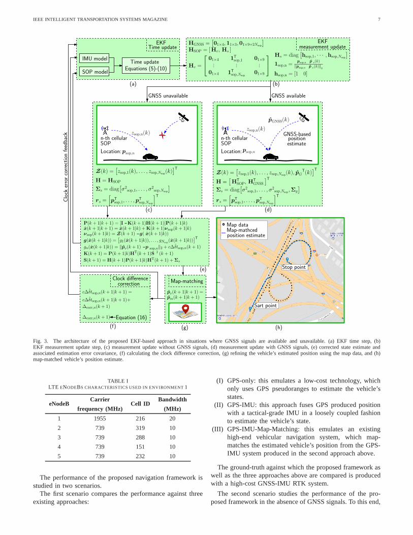
cellular SOP transmitters with fully known locations. Theframework provides a robust and accurate navigation with andwithout GNSS signals by exploiting ambient cellular SOPs. Incontrast to traditional approaches, which employ an integratedGNSS-IMU systems with a digital map, the proposed frame-work deals with a unknown dynamic, stochastic error statesof cellular SOPs by simultaneously estimating them. Theseestimates are further refined via a closed-loop map-matchingstep. The EKF time and measurement update steps are outlinednext, followed by the map-matching correction step.

A. EKF Time Update

In this subsection, the EKF time update step is described.The EKF’s vectorx consists of the vehicle’s statexv (1) andthe clock error states (6), i.e.,

x =[

xT

v ,xT

clk,sop

]T

.

The cellular SOPs are assumed to be stationary withknown positions

psop,n

Nsop

n=1. Between measurement updates

(whether from GNSS or cellular signals), the IMU’s sampledmeasurements of the angular velocityω and linear accel-eration a are used to perform a time update ofx(k|j) ,

E

[

x(k)∣

∣

∣z(i)

j

i=1

]

, for k > j to get the predicted states

x(k + 1|j) and corresponding prediction error covarianceP(k + 1|j). The time update of the orientation state estimateis given by

Ik+1|j

Gˆq =

Ik+1

Ikˆq ⊗

Ik|j

Gˆq, (8)

where Ik+1

Ikˆq represents the estimated relative rotation of the

IMU from time-step k to k + 1. In (8), ⊗ denotes thequaternion multiplication operator, which operates on twoquaternion vectorsq1 , [q0,1, qv1,1, qv2,1, qv3,1] and q2 ,

[q0,2, qv1,2, qv2,2, qv3,2] to yield

q1 ⊗ q2 = [q0,1q0,2 − qv1,1qv1,2 − qv2,1qv2,2 − qv3,1qv3,2,

q0,1qv1,2 + qv1,1q0,2 + qv2,1qv3,2 − qv3,1qv2,2,

q0,1qv2,2 − qv1,1qv3,2 + qv2,1q0,2 + qv3,1qv1,2,

q0,1qv3,2 + qv1,1qv2,2 − qv2,1qv3,2 + qv3,1q0,2 ]T.

The value ofIk+1

Ikˆq is found by integrating the measurements

ω(k) andω(k + 1) using a fourth order Runge-Kutta, whichyields

Ik+1

Ikˆq = q0 +

T

2(d1 + 2d2 + 2d3 + d4) ,

d1 =1

2Ω (ω(k)) q0, d2 =

1

2Ω(

ˆω(k))

(

q0 +1

2Td1

)

,

d3 =1

2Ω(

ˆω(k))

(

q0 +1

2Td2

)

,

d4 =1

2Ω (ω(k + 1))

(

q0 +1

2Td3

)

,

ˆω(k) =1

2(ω(k) + ω(k + 1)) , q0 = [ 1, 0, 0, 0]

T,

whereω = ω − bg and

Ω(ω) =

[

0 ωT

ω ⌊ω×⌋

]

,

⌊ω×⌋ =

0 −ωz ωy

ωz 0 −ωx

−ωy ωx 0

, ω = [ωx, ωy, ωz]T.

The time update of the velocity estimate is computed usingthe trapezoidal integration according to

ˆpv(k+1|j) = ˆpv(k|j)+T

2[s(k) + s(k + 1)]+T Gg(k), (9)

where s(k) , RT

q (k)a(k), a(k) , a(k) − ba(k|j) and

Rq(k) , R[

Ik|j

Gˆq]

. The time update of the position estimateis given by

pv(k + 1|j) = pv(k|j) +T

2

[

ˆpv(k + 1|j) + ˆpv(k|j)]

. (10)

The time update of the gyroscope and accelerometer biasesestimates is given by

bg(k + 1|j) = bg(k|j), ba(k + 1|j) = ba(k|j). (11)

The time update of the clock error state estimate is readilydeduced from (7) to be given by

xclk,sop(k + 1|j) = Φclkxclk,sop(k|j). (12)

The time update of the prediction error covariance is given by

P(k + 1|j) = F(k)P(k|j)FT(k) +Q(k), (13)

F(k) , diag [ΦB(k + 1, k), Φclk] ,

Q(k) , diag [QdB(k), Qclk,sop] .

The discrete-time INS state transition matrixΦB and processnoise covarianceQdB

are computed using standard INS equa-tions as described in [33], [34].

B. EKF Measurement Update

When GNSS signals are available, the EKF measurementupdate stage corrects the time updated states with (i) cellularSOP pseudoranges, (ii) digital map data, and (iii) the esti-mated vehicle’s position obtained from the GNSS navigationsolutionpGNSS , [pGNSSx

, pGNSSy, pGNSSz

]T. Here, the mea-surement vectorZ(k) consists ofpGNSS and zsop,n

Nsop

n=1,

where zsop,n is the pseudorange drawn from then-th cel-lular SOP transmitter. The error of the estimated positionobtained from the GNSS navigation solution is modeledas a zero-mean Gaussian random vector with a covarianceΣg = diag

[

σ2GNSS,x, σ

2GNSS,y, σ

2GNSS,z

]

. When GNSSsignals become unavailable, the measurement update stageonly uses (i) cellular SOP pseudoranges and (ii) digital mapdata. Here,Z(k) only includes cellular SOP measurements,zsop,n

Nsop

n=1.

Next, the corrected state estimatex(k+1|k+1) and associ-ated estimation error covarianceP(k + 1|k + 1) is computedusing the standard EKF measurement update equations [23].The expressions of the corresponding measurement JacobianH and the measurement noise covarianceΣs are demonstratedin Fig. 3.

IEEE INTELLIGENT TRANSPORTATION SYSTEMS MAGAZINE 6

C. Map-Matching and Closed-Loop Clock Error State Cor-rection

Assuming that the digital map comprisesLN locations, de-

noted

ln , [pmxn, pmyn

, pmzn]TLN

n=1, the position estimate

pv(k|k) is map-matched to yieldpm(k|k) according to

pm(k + 1|k + 1) = minln‖pv(k + 1|k + 1)− ln‖Σm

, (14)

where

‖pv(k + 1|k + 1)− ln‖Σm=

√

[pv(k + 1|k + 1)− ln]TΣm−1[pv(k + 1|k + 1)− ln].

The estimatespv(k+1|k+1) andpm(k+1|k+1) are fedback to correct the clock bias state estimates according to

c∆δtsop,n(k + 1|k + 1)←−c∆δtsop,n(k + 1|k + 1)

+ ∆corr,n(k + 1), (15)

where

∆corr,n(k + 1) =‖pv(k + 1|k + 1)− psop,n‖2

− ‖pm(k + 1|k + 1)− psop,n‖2. (16)

Finally, the map-matched estimatepm(k+1|k+1) is usedto replace the estimatepv(k + 1|k + 1), i.e.,

pv(k + 1|k + 1)←− pm(k + 1|k + 1).

Fig. 3 summarizes the architecture of the proposed naviga-tion framework.

IV. EXPERIMENTAL RESULTS

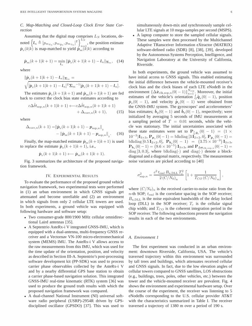
To evaluate the performance of the proposed ground vehiclenavigation framework, two experimental tests were performedin (1) an urban environment in which GNSS signals getattenuated and become unreliable and (2) an environmentin which signals from only 2 cellular LTE towers are used.In both experiments, a ground vehicle was equipped withfollowing hardware and software setup:

• Two consumer-grade 800/1900 MHz cellular omnidirec-tional Laird antennas [35].

• A Septentrio AsteRx-i V integrated GNSS-IMU, which isequipped with a dual-antenna, multi-frequency GNSS re-ceiver and a Vectornav VN-100 micro-electromechanicalsystem (MEMS) IMU. The AsteRx-i V allows access tothe raw measurements from this IMU, which was used forthe time update of the orientation, position, and velocityas described in Section III-A. Septentrio’s post-processingsoftware development kit (PP-SDK) was used to processcarrier phase observables collected by the AsteRx-i Vand by a nearby differential GPS base station to obtaina carrier phase-based navigation solution. This integratedGNSS-IMU real-time kinematic (RTK) system [36] wasused to produce the ground truth results with which theproposed navigation framework was compared.

• A dual-channel National Instrument (NI) universal soft-ware radio peripheral (USRP)-2954R driven by GPS-disciplined oscillator (GPSDO) [37]. This was used to

simultaneously down-mix and synchronously sample cel-lular LTE signals at 10 mega-samples per second (MSPS).

• A laptop computer to store the sampled cellular signals.These samples were then processed by the MultichannelAdaptive TRansceiver Information eXtractor (MATRIX)software-defined radio (SDR) [8], [38], [39], developedby the Autonomous Systems Perception, Intelligence, andNavigation Laboratory at the University of California,Riverside.

In both experiments, the ground vehicle was assumed tohave initial access to GNSS signals. This enabled estimatingthe initial difference between the vehicle-mounted receiver’sclock bias and the clock biases of each LTE eNodeB in theenvironment∆xclk,sop,n(0| − 1)

Nsop

n=1. Moreover, the initial

estimates of the vehicle’s orientationIGˆqv(0| − 1), positionpv(0| − 1), and velocity ˆpv(0| − 1) were obtained fromthe GNSS-IMU system. The gyroscopes’ and accelerometers’bias estimates;bg(0| − 1) and ba(0| − 1), respectively; wereinitialized by averaging 5 seconds of IMU measurements ata sampling period ofT = 0.01 seconds, while the vehi-cle was stationary. The initial uncertainties associated withthese state estimates were set toPI

Gqv(0| − 1) = (1 ×

10−3)I3×3, Ppv(0| − 1) = blkdiag [3 I2×2, 0], Ppv

(0| − 1) =blkdiag [0.5 I2×2, 0], Pbg

(0| − 1) =(

3.75× 10−9)

I3×3,Pba

(0| − 1) =(

9.6× 10−5)

I3×3, andP∆xclk,sop,n(0| − 1) =

diag [3, 0.3], where blkdiag(·) and diag(·) denote a block-diagonal and a diagonal matrix, respectively. The measurementnoise variances are picked according to [40]

σ2sop,n =

c2 temlBn,DLL T2c

2 (C/N0)n

[

1 +1

TCO (C/N0)n

]

,

where(C/N0)n is the received carrier-to-noise ratio from then-th SOP;teml is the correlator spacing in the SOP receiver;Bn,DLL is the noise equivalent bandwidth of the delay lockedloop (DLL) in the SOP receiver;Tc is the cellular signalchip width; andTCO is the coherent integration period in theSOP receiver. The following subsections present the navigationresults in each of the two environments.

A. Environment 1

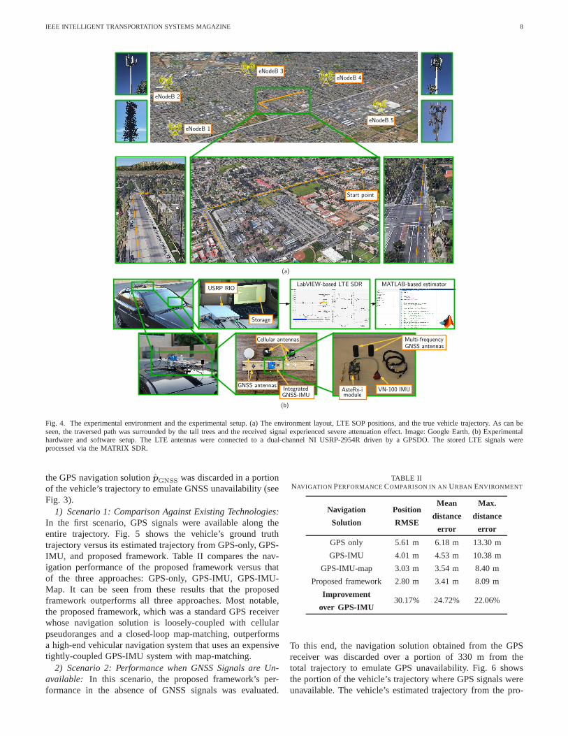
The first experiment was conducted in an urban environ-ment: downtown Riverside, California, USA. The vehicle’straversed trajectory within this environment was surroundedby tall trees and buildings, which attenuates received cellularand GNSS signals. In fact, due to the low elevation angles ofcellular towers compared to GNSS satellites, LOS obstructions(e.g., buildings, trees, poles, other vehicles, etc.) between thetower and the vehicle-mounted receiver are prevalent. Fig.4shows the environment and experimental hardware setup. Overthe course of the experiment, the receiver was listening to 5eNodeBs corresponding to the U.S. cellular provider AT&Twith the characteristics summarized in Table I. The receivertraversed a trajectory of 1380 m over a period of 190 s.

IEEE INTELLIGENT TRANSPORTATION SYSTEMS MAGAZINE 7

EKF

IMU model

Time update

SOP model

EKFmeasurement update

Location:

pGNSS(k)

GNSS-basedpositionn-th cellular

Location:psop;n

rs =h

pT

sop;1; : : : ;pT

sop;Nsop

iT

Σs = diag[

σ2sop;1; : : : ; σ

2sop;Nsop

]

Z(k) =[

zsop;1(k); : : : ; zsop;Nsop(k)

]T

zsop;n(k)

GNSS unavailable GNSS available

pv(k + 1jk + 1) =

Map-matchingClock differencecorrection

c∆δtsop;n(k + 1jk + 1) =

c∆δtsop;n(k + 1jk + 1)+Sart point

Stop point

Map-mathcedMap data

Clock

errorcorrection

feedback

(a) (b)

(c) (d)

(e)

(f) (g) (h)

HSOP = [Hv; Hs ]

Hv =

2

4

01×4 1T

sop;1 01×9... ... ...

01×4 1T

sop;Nsop01×9

3

5

1sop;n =psop;n p v

(k)

kpsop;n p v(k)k

2

Hs = diag[

hsop;1; · · · ;hsop;Nsop

]

hsop;n = [1 0]

HGNSS =[

01×4;11×3;01×9+2Nsop

]

H = HSOP H =[

HT

SOP; HT

GNSS

]T

P(k + 1jk + 1) = [I K(k + 1)H(k + 1)]P(k + 1jk)x(k + 1jk + 1) = x(k + 1jk) +K(k + 1)νsop(k + 1jk)

Equations (5)-(10)Time update

SOPn-th cellularSOP

position estimate

estimate

Z(k) =[

zsop;1(k); : : : ; zsop;Nsop(k); pG

T(k)]T

zsop;n(k)

psop;n

Σs = diag[

σ2sop;1; : : : ; σ

2sop;Nsop

;Σg

]

rs =h

pT

sop;1; : : : ;pT

sop;Nsop

iT

νsop(k + 1jk) = Z(k + 1) g( x(k + 1jk))

K(k + 1) = P(k + 1jk)HT(k + 1)S1 (k + 1)

S(k + 1) = H(k + 1)P(k + 1jk)HT(k + 1) +Σs

gn(x(k + 1jk)) = kpv(k + 1) p sop;nk2 + c∆δtsop;n(k + 1)

g(x(k + 1jk)) =[

g1(x(k + 1jk)); : : : ; gNsop(x(k + 1jk))

]T

∆corr;n(k + 1)

∆corr;n(k + 1) Equation (16)

pm(k + 1jk + 1)

Fig. 3. The architecture of the proposed EKF-based approachin situations where GNSS signals are available and unavailable. (a) EKF time step, (b)EKF measurement update step, (c) measurement update without GNSS signals, (d) measurement update with GNSS signals, (e) corrected state estimate andassociated estimation error covariance, (f) calculating the clock difference correction, (g) refining the vehicle’s estimated position using the map data, and (h)map-matched vehicle’s position estimate.

TABLE ILTE ENODEBS CHARACTERISTICS USED IN ENVIRONMENT1

eNodeBCarrier

frequency (MHz)Cell ID

Bandwidth

(MHz)

1 1955 216 20

2 739 319 10

3 739 288 10

4 739 151 10

5 739 232 10

The performance of the proposed navigation framework isstudied in two scenarios.

The first scenario compares the performance against threeexisting approaches:

(I) GPS-only: this emulates a low-cost technology, whichonly uses GPS pseudoranges to estimate the vehicle’sstates.

(II) GPS-IMU: this approach fuses GPS produced positionwith a tactical-grade IMU in a loosely coupled fashionto estimate the vehicle’s state.

(III) GPS-IMU-Map-Matching: this emulates an existinghigh-end vehicular navigation system, which map-matches the estimated vehicle’s position from the GPS-IMU system produced in the second approach above.

The ground-truth against which the proposed framework aswell as the three approaches above are compared is producedwith a high-cost GNSS-IMU RTK system.

The second scenario studies the performance of the pro-posed framework in the absence of GNSS signals. To this end,

IEEE INTELLIGENT TRANSPORTATION SYSTEMS MAGAZINE 8

eNodeB 1

eNodeB 2

eNodeB 3eNodeB 4

eNodeB 5

MATLAB-based estimator

Cellular antennas

Start point

LabVIEW-based LTE SDRUSRP RIO

Storage

(a)

(b)

GNSS antennas

Multi-frequencyGNSS antennas

VN-100 IMUAsteRx-imodule

IntegratedGNSS-IMU

Fig. 4. The experimental environment and the experimental setup. (a) The environment layout, LTE SOP positions, and thetrue vehicle trajectory. As can beseen, the traversed path was surrounded by the tall trees andthe received signal experienced severe attenuation effect. Image: Google Earth. (b) Experimentalhardware and software setup. The LTE antennas were connected to a dual-channel NI USRP-2954R driven by a GPSDO. The stored LTE signals wereprocessed via the MATRIX SDR.

the GPS navigation solutionpGNSS was discarded in a portionof the vehicle’s trajectory to emulate GNSS unavailability(seeFig. 3).

1) Scenario 1: Comparison Against Existing Technologies:In the first scenario, GPS signals were available along theentire trajectory. Fig. 5 shows the vehicle’s ground truthtrajectory versus its estimated trajectory from GPS-only,GPS-IMU, and proposed framework. Table II compares the nav-igation performance of the proposed framework versus thatof the three approaches: GPS-only, GPS-IMU, GPS-IMU-Map. It can be seen from these results that the proposedframework outperforms all three approaches. Most notable,the proposed framework, which was a standard GPS receiverwhose navigation solution is loosely-coupled with cellularpseudoranges and a closed-loop map-matching, outperformsa high-end vehicular navigation system that uses an expensivetightly-coupled GPS-IMU system with map-matching.

2) Scenario 2: Performance when GNSS Signals are Un-available: In this scenario, the proposed framework’s per-formance in the absence of GNSS signals was evaluated.

TABLE IINAVIGATION PERFORMANCECOMPARISON IN AN URBAN ENVIRONMENT

Navigation

Solution

Position

RMSE

Mean

distance

error

Max.

distance

error

GPS only 5.61 m 6.18 m 13.30 m

GPS-IMU 4.01 m 4.53 m 10.38 m

GPS-IMU-map 3.03 m 3.54 m 8.40 m

Proposed framework 2.80 m 3.41 m 8.09 m

Improvement

over GPS-IMU30.17% 24.72% 22.06%

To this end, the navigation solution obtained from the GPSreceiver was discarded over a portion of 330 m from thetotal trajectory to emulate GPS unavailability. Fig. 6 showsthe portion of the vehicle’s trajectory where GPS signals wereunavailable. The vehicle’s estimated trajectory from the pro-

IEEE INTELLIGENT TRANSPORTATION SYSTEMS MAGAZINE 9

GPS-IMUGPS-onlyGround truth

Proposed framework

Fig. 5. Experimental results in an urban environment. The vehicle’s estimatedtrajectory with our proposed framework is compared againstthe estimatedtrajectory with a GPS-only and a GPS-IMU system. The ground-truth wasobtained with an expensive GPS-IMU system with RTK. Experimental resultsindicate a 2.80 m RMSE for the proposed approach. Image: Google Earth

posed framework is also shown versus the vehicle’s estimatedtrajectory from the GPS-IMU system. Table III compares thenavigation performance of the proposed framework versus thatof the GPS-IMU system. As expected, when GPS signals wereunavailable, the IMU’s solution drifted due to the lack ofaiding corrections from GPS signals. The error accumulationdue to this drift is particularly hazardous for semi-autonomousor fully autonomous ground vehicles. In contrast, our proposedframework did not exhibit such drift as cellular signals wereused as an aiding source to the IMU.

Ground truthGPS-IMU

GPS unavailableGPS available

Proposed framework

Fig. 6. Vehicle’s estimated trajectory from the GPS-IMU system versus ourproposed framework when GPS signals become unavailable andthen availableare specified. As can be seen, the GPS-IMU solution drifts in the absence ofGPS signals. In contrast, our proposed framework does not exhibit such driftas cellular signals are used as an aiding source to the IMU. Image: GoogleEarth.

B. Environment 2

The second experiment was conducted in an urban envi-ronment: downtown Riverside, California, USA. Here, only2 LTE SOP towers were used to assess the performance ofour proposed framework in the case where a small number ofcellular towers are available. Over the course of the experi-ment, the vehicle-mounted receiver traversed a total trajectory

TABLE IIINAVIGATION PERFORMANCECOMPARISON WITHOUTGPSSIGNALS

Navigation

Solution

Position

RMSE

Mean

distance

error

Max.

distance

error

GPS-IMU 8.37 m 14.87 m 57.12 m

Proposed framework 3.12 m 4.22 m 10.67 m

Improvement

over GPS-IMU62.72% 71.6% 81.32%

of 510 m while simultaneously listening to 2 LTE SOPscorresponding to the U.S. cellular providers T-Mobile andAT&T. Table IV summarizes the LTE eNodeBs characteristicsused in Experiment 2.

TABLE IVLTE ENODEBS CHARACTERISTICS USED IN ENVIRONMENT2

LTE

SOPOperator

Carrier

frequency (MHz)Cell ID

Bandwidth

(MHz)

1 T-Mobile 2145 79 20

2 AT&T 1955 350 20

Fig. 7 shows the experimental environment, the locationof the LTE towers, and the vehicle’s ground truth trajectoryversus that estimated with the proposed framework and thatestimated with the GPS-IMU system. To evaluate the perfor-mance of the proposed framework in the absence of GNSSsignals, while using signals from only 2 LTE SOPs, the nav-igation solution obtained from the GPS receiver is discardedover a portion of 40 m of the total trajectory to emulate GPSunavailability. Table V summarizes the navigation performancein this environment. It can be seen that the proposed approachyielded a 32% reduction in the position RMSE and a 43%reduction in the maximum distance error, despite using a verylimited number of cellular SOPs.

TABLE VNAVIGATION PERFORMANCECOMPARISON WITHOUTGPSSIGNALS

Navigation

Solution

Position

RMSE

Mean

distance

error

Max.

distance

error

GPS-IMU 5.10 m 4.75 m 8.96 m

Proposed framework 3.43 m 4.18 m 5.03 m

Improvement

over GPS-IMU32% 18% 43%

V. CONCLUSION

This article presented a novel framework for vehicularnavigation in urban environments. The framework uses anIMU, cellular signals, and GNSS signals (when available),along with closed-loop map-matching. On one hand, when

IEEE INTELLIGENT TRANSPORTATION SYSTEMS MAGAZINE 10

eNodeB 1

Start point

eNodeB 2

Start pointStop point

GPS cutoff

GPS back inRMSE = 3.43 m

RMSE = 5.1 m

Ground truthGPS-IMUProposed framework

GPS-IMU

Proposed framework

Fig. 7. The second experimental environment layout, LTE SOPpositions, truevehicle trajectory, and the different navigation solutions, where the estimatedvehicle position obtained from GPS-IMU and the proposed method are shownusing yellow and red lines, respectively. Over the course ofthe experiment,the vehicle-mounted receiver traversed a total trajectoryof 510 m in anurban streets while listening to only 2 LTE SOPs simultaneously. It is worthmentioning that in the experiment area, the LTE towers were obstructed bythe buildings and the first LTE tower was far from the vehicle,and a largeportion of the vehicle’s trajectory had no clear LOS to this LTE towers. As canbe seen, the estimated position using the proposed framework follows closelythe ground truth trajectory during the drive. Experimentalresults indicate a3.43 m RMSE for the proposed approach. Image: Google Earth.

GNSS signals are unavailable, the proposed framework usescellular signals as an aiding source to the IMU, bounding theIMU drift, and producing an accurate estimate of the vehicle’sstate. On the other hand, when GNSS signals are available,the proposed framework fuses estimates from the GNSSreceiver with cellular measurements to produce an estimatethat is within a few meters of the estimate produced by avery expensive, high-end GNSS-IMU system with RTK andmap-matching. Experimental results in 2 urban environmentsare presented demonstrating the accuracy of the proposedframework versus existing technologies. It was demonstratedthat the proposed framework achieved a position RMSE of2.8 m over a trajectory of 1380 m while GNSS signals wereavailable and a position RMSE of 3.12 over the same trajectorywhile GNSS signals were not available for 330 m. In addition,the robustness of the proposed framework to having a limitednumber of cellular towers (only 2) was demonstrated, showinga position RMSE of 3.43 m over a trajectory of 510 m, duringwhich GNSS signals were unavailable for 40 m.

REFERENCES

[1] R. Toledo-Moreo, D. Betaille, and F. Peyret, “Lane-level integrityprovision for navigation and map matching with GNSS, dead reckoning,and enhanced maps,”IEEE Transactions on Intelligent TransportationSystems, vol. 11, no. 1, pp. 100–112, March 2010.

[2] M. Rohani, D. Gingras, and D. Gruyer, “A novel approach for improvedvehicular positioning using cooperative map matching and dynamic basestation dgps concept,”IEEE Transactions on Intelligent TransportationSystems, vol. 17, no. 1, pp. 230–239, January 2016.

[3] M. Hashemi, “Reusability of the output of map-matching algorithmsacross space and time through machine learning,”IEEE Transactionson Intelligent Transportation Systems, vol. 18, no. 11, pp. 3017–3026,November 2017.

[4] A. Ramanandan, A. Chen, and J. Farrell, “Inertial navigation aidingby stationary updates,”IEEE Transactions on Intelligent TransportationSystems, vol. 13, no. 1, pp. 235–248, March 2012.

[5] A. Vu, A. Ramanandan, A. Chen, J. Farrell, and M. Barth, “Real-timecomputer vision/DGPS-aided inertial navigation system for lane-levelvehicle navigation,”IEEE Transactions on Intelligent TransportationSystems, vol. 13, no. 2, pp. 899–913, June 2012.

[6] G. De Angelis, G. Baruffa, and S. Cacopardi, “GNSS/cellular hybridpositioning system for mobile users in urban scenarios,”IEEE Transac-tions on Intelligent Transportation Systems, vol. 14, no. 1, pp. 313–321,March 2013.

[7] M. Driusso, C. Marshall, M. Sabathy, F. Knutti, H. Mathis, andF. Babich, “Vehicular position tracking using LTE signals,” IEEE Trans-actions on Vehicular Technology, vol. 66, no. 4, pp. 3376–3391, April2017.

[8] K. Shamaei, J. Khalife, and Z. Kassas, “Exploiting LTE signals fornavigation: Theory to implementation,”IEEE Transactions on WirelessCommunications, vol. 17, no. 4, pp. 2173–2189, April 2018.

[9] J. Khalife and Z. Kassas, “Navigation with cellular CDMAsignals – partII: Performance analysis and experimental results,”IEEE Transactionson Signal Processing, vol. 66, no. 8, pp. 2204–2218, April 2018.

[10] J. McEllroy, “Navigation using signals of opportunityin the AMtransmission band,” Master’s thesis, Air Force Institute of Technology,Wright-Patterson Air Force Base, Ohio, USA, 2006.

[11] S. Fang, J. Chen, H. Huang, and T. Lin, “Is FM a RF-based positioningsolution in a metropolitan-scale environment? A probabilistic approachwith radio measurements analysis,”IEEE Transactions on Broadcasting,vol. 55, no. 3, pp. 577–588, September 2009.

[12] Z. Kassas, “Collaborative opportunistic navigation,” IEEE Aerospaceand Electronic Systems Magazine, vol. 28, no. 6, pp. 38–41, 2013.

[13] Z. Kassas, “Analysis and synthesis of collaborative opportunistic navi-gation systems,” Ph.D. dissertation, The University of Texas at Austin,USA, 2014.

[14] 3GPP2, “Physical layer standard for cdma2000 spread spectrum sys-tems (C.S0002-E),” 3rd Generation Partnership Project 2 (3GPP2), TSC.S0002-E, June 2011.

[15] J. Khalife, K. Shamaei, and Z. Kassas, “A software-defined receiverarchitecture for cellular CDMA-based navigation,” inProceedings ofIEEE/ION Position, Location, and Navigation Symposium, April 2016,pp. 816–826.

[16] J. Khalife, K. Shamaei, and Z. Kassas, “Navigation withcellular CDMAsignals – part I: Signal modeling and software-defined receiver design,”IEEE Transactions on Signal Processing, vol. 66, no. 8, pp. 2191–2203,April 2018.

[17] 3GPP, “Evolved universal terrestrial radio access (E-UTRA);physical channels and modulation,” 3rd Generation PartnershipProject (3GPP), TS 36.211, January 2011. [Online]. Available:http://www.3gpp.org/ftp/Specs/html-info/36211.htm

[18] K. Shamaei, J. Khalife, and Z. Kassas, “Performance characterization ofpositioning in LTE systems,” inProceedings of ION GNSS Conference,September 2016, pp. 2262–2270.

[19] K. Shamaei, J. Khalife, S. Bhattacharya, and Z. Kassas,“Computation-ally efficient receiver design for mitigating multipath forpositioningwith LTE signals,” inProceedings of ION GNSS Conference, September2017, pp. 3751–3760.

[20] Z. Kassas, V. Ghadiok, and T. Humphreys, “Adaptive estimation ofsignals of opportunity,” inProceedings of ION GNSS Conference,September 2014, pp. 1679–1689.

[21] J. Morales and Z. Kassas, “Optimal collaborative mapping of terres-trial transmitters: receiver placement and performance characterization,”IEEE Transactions on Aerospace and Electronic Systems, vol. 54, no. 2,pp. 992–1007, April 2018.

[22] Z. Kassas and T. Humphreys, “Observability analysis ofcollaborativeopportunistic navigation with pseudorange measurements,” IEEE Trans-actions on Intelligent Transportation Systems, vol. 15, no. 1, pp. 260–273, February 2014.

[23] Y. Bar-Shalom, X. Li, and T. Kirubarajan,Estimation with Applicationsto Tracking and Navigation. New York, NY: John Wiley & Sons, 2002.

[24] A. Thompson, J. Moran, and G. Swenson,Interferometry and Synthesisin Radio Astronomy, 2nd ed. John Wiley & Sons, 2001.

[25] J. Barnes, A. Chi, R. Andrew, L. Cutler, D. Healey, D. Leeson,T. McGunigal, J. Mullen, W. Smith, R. Sydnor, R. Vessot, and G. Win-kler, “Characterization of frequency stability,”IEEE Transactions on

IEEE INTELLIGENT TRANSPORTATION SYSTEMS MAGAZINE 11

Instrumentation and Measurement, vol. 20, no. 2, pp. 105–120, May1971.

[26] R. Brown and P. Hwang,Introduction to Random Signals and AppliedKalman Filtering, 3rd ed. John Wiley & Sons, 2002.

[27] M. Atia, A. Hilal, C. Stellings, E. Hartwell, J. Toonstra, W. Miners,and O. Basir, “A low-cost lane-determination system using GNSS/IMUfusion and HMM-based multistage map matching,”IEEE Transactionson Intelligent Transportation Systems, vol. 18, no. 11, pp. 3027–3037,November 2017.

[28] G. Jagadeesh and T. Srikanthan, “Online map-matching of noisy andsparse location data with hidden Markov and route choice models,” IEEETransactions on Intelligent Transportation Systems, vol. 18, no. 9, pp.2423–2434, September 2017.

[29] Z. Peng, S. Gao, B. Xiao, S. Guo, and Y. Yang, “CrowdGIS: Updatingdigital maps via mobile crowdsensing,”IEEE Transactions on Automa-tion Science and Engineering, vol. PP, no. 99, pp. 1–12, 2017.

[30] Open Street Map foundation (OSMF). [Online]. Available:https://www.openstreetmap.org

[31] P. Bender, J. Ziegler, and C. Stiller, “Lanelets: Efficient map repre-sentation for autonomous driving,” inProceedings of IEEE IntelligentVehicles Symposium Proceedings, June 2014, pp. 420–425.

[32] F. Li, P. Bonnifait, J. Ibanez-Guzman, and C. Zinoune, “Lane-level map-matching with integrity on high-definition maps,” inProceedings ofIEEE Intelligent Vehicles Symposium, June 2017, pp. 1176–1181.

[33] J. Farrell and M. Barth,The Global Positioning System and InertialNavigation. New York: McGraw-Hill, 1998.

[34] P. Groves,Principles of GNSS, Inertial, and Multisensor IntegratedNavigation Systems, 2nd ed. Artech House, 2013.

[35] Laird phantom 3G/4G multiband antenna NMOmount white TRA6927M3NB. [Online]. Available:https://www.lairdtech.com/products/phantom-series-antennas

[36] Septentrio AsteRx-i V. [Online]. Available:https://www.septentrio.com/products/gnss-receivers/rover-base-receivers/oem-receiver-boards

[37] National instrument universal software radio peripheral-2954r. [Online].Available: http://www.ni.com/en-us/support/model.usrp-2954.html

[38] Z. Kassas, J. Khalife, K. Shamaei, and J. Morales, “I hear, thereforeI know where I am: Compensating for GNSS limitations with cellularsignals,” IEEE Signal Processing Magazine, pp. 111–124, September2017.

[39] K. Shamaei and Z. Kassas, “LTE receiver design and multipath analysisfor navigation in urban environments,”NAVIGATION, Journal of theInstitute of Navigation, 2018, accepted.

[40] P. Misra and P. Enge,Global Positioning System: Signals, Measurements,and Performance, 2nd ed. Ganga-Jamuna Press, 2010.

Zaher (Zak) M. Kassas (S’98-M’08-SM’11) is anassistant professor at the University of California,Riverside (UCR) and director of the AutonomousSystems Perception, Intelligence, and Navigation(ASPIN) Laboratory. He received a B.E. in ElectricalEngineering from the Lebanese American Univer-sity, an M.S. in Electrical and Computer Engineeringfrom The Ohio State University, and an M.S.E. inAerospace Engineering and a Ph.D. in Electrical andComputer Engineering from The University of Texasat Austin. In 2018, he received the NSF Faculty

Early Career Development Program (CAREER) award. His research inter-ests include cyber-physical systems, estimation theory, navigation systems,autonomous vehicles, and intelligent transportation systems.

Mahdi Maaref is a postdoctoral research fellowat UCR. He received the B.E degree in ElectricalEngineering from the University of Tehran in 2008and M.Sc. degree in Electrical Engineering-PowerSystem at the same University in 2011 and Ph.D.Degree in Electrical Engineering at Shahid BeheshtiUniversity, Tehran, Iran in 2016. He was a visitingresearch collaborator at the University of Alberta,Edmonton, Canada in 2016. His main interest is onopportunistic perception, distributed estimation andreal-time systems.

Joshua J. Morales (S’11) is a Ph.D. candidate atUCR and a member of the ASPIN Laboratory. He re-ceived a B.S. in ECE with High Honors from UCR.His research interests include estimation, navigation,autonomous vehicles, and intelligent transportationsystems.

Joe J. Khalife (S’15) is a Ph.D. candidate at UCRand a member of the ASPIN Laboratory. He receiveda B.E. in EE and an M.S. in Computer Engineeringfrom LAU. His research interests include opportunis-tic navigation, autonomous vehicles, and SDR.

Kimia Shamaei (S’15) is a Ph.D. candidate at UCRand a member of the ASPIN Laboratory. She re-ceived a B.S. and an M.S. in EE from the Universityof Tehran. Her current research interests includeanalysis and modeling of signals of opportunity andSDR.