Robust Semantic Text Similarity Using LSA, Machine ... Kashyap · Lushan Han · Roberto Yus ·...

Language Resources and Evaluation: PreprintFinal publication is available at Springer via http://dx.doi.org/10.1007/s10579-015-9319-2

Robust Semantic Text Similarity Using LSA, Machine

Learning, and Linguistic Resources

Abhay Kashyap · Lushan Han · RobertoYus · Jennifer Sleeman · TaneeyaSatyapanich · Sunil Gandhi · Tim Finin

Received: 2014-11-09 / Accepted: 2015-10-19

Abstract Semantic textual similarity is a measure of the degree of semantic equiv-alence between two pieces of text. We describe the SemSim system and its perfor-mance in the *SEM 2013 and SemEval-2014 tasks on semantic textual similarity.At the core of our system lies a robust distributional word similarity compo-nent that combines Latent Semantic Analysis and machine learning augmentedwith data from several linguistic resources. We used a simple term alignment algo-rithm to handle longer pieces of text. Additional wrappers and resources were usedto handle task specific challenges that include processing Spanish text, compar-ing text sequences of di↵erent lengths, handling informal words and phrases, andmatching words with sense definitions. In the *SEM 2013 task on Semantic Tex-tual Similarity, our best performing system ranked first among the 89 submittedruns. In the SemEval-2014 task on Multilingual Semantic Textual Similarity, weranked a close second in both the English and Spanish subtasks. In the SemEval-2014 task on Cross–Level Semantic Similarity, we ranked first in Sentence–Phrase,Phrase–Word, and Word–Sense subtasks and second in the Paragraph–Sentencesubtask.

Keywords Latent Semantic Analysis · WordNet · term alignment · semanticsimilarity

1 Introduction

Semantic Textual Similarity (STS) is a measure of how close the meanings oftwo text sequences are [4]. Computing STS has been a research subject in natu-ral language processing, information retrieval, and artificial intelligence for manyyears. Previous e↵orts have focused on comparing two long texts (e.g., for doc-ument classification) or a short text with a long one (e.g., a search query anda document), but there are a growing number of tasks that require computing

Abhay Kashyap, Lushan Han, Jennifer Sleeman, Taneeya Satyapanich, Sunil Gandhi, and TimFinin, University of Maryland, Baltimore County (USA), E-mail: {abhay1, lushan1, jsleem1,taneeya1, sunilga1, finin}@umbc.edu; Roberto Yus, University of Zaragoza (Spain), E-mail:[email protected]

2 Abhay Kashyap et al.

the semantic similarity between two sentences or other short text sequences. Forexample, paraphrase recognition [15], tweets search [49], image retrieval by cap-tions [11], query reformulation [38], automatic machine translation evaluation [30],and schema matching [21,19,22], can benefit from STS techniques.

There are three predominant approaches to computing short text similarity.The first uses information retrieval’s vector space model [36] in which each pieceof text is modeled as a “bag of words” and represented as a sparse vector of wordcounts. The similarity between two texts is then computed as the cosine similarityof their vectors. A variation on this approach leverages web search results (e.g.,snippets) to provide context for the short texts and enrich their vectors using thewords in the snippets [47]. The second approach is based on the assumption that iftwo sentences or other short text sequences are semantically equivalent, we shouldbe able to align their words or expressions by meaning. The alignment qualitycan serve as a similarity measure. This technique typically pairs words from thetwo texts by maximizing the summation of the semantic similarity of the resultingpairs [40]. The third approach combines di↵erent measures and features usingmachine learning models. Lexical, semantic, and syntactic features are computedfor the texts using a variety of resources and supplied to a classifier, which assignsweights to the features by fitting the model to training data [48].

In this paper we describe SemSim, our semantic textual similarity system. Ourapproach uses a powerful semantic word similarity model based on a combinationof latent semantic analysis (LSA) [14,31] and knowledge from WordNet [42]. For agiven pair of text sequences, we align terms based on our word similarity model tocompute its overall similarity score. Besides this completely unsupervised model, italso includes supervised models from the given SemEval training data that combinethis score with additional features using support vector regression. To handle textin other languages, e.g., Spanish sentence pairs, we use Google Translate API1 totranslate the sentences into English as a preprocessing step. When dealing withuncommon words and informal words and phrases, we use the Wordnik API2 andthe Urban Dictionary to retrieve their definitions as additional context.

The SemEval tasks for Semantic Textual Similarity measure how well auto-matic systems compute sentence similarity for a set of text sequences according toa scale definition ranging from 0 to 5, with 0 meaning unrelated and 5 meaningsemantically equivalent [4,3]. For the SemEval-2014 workshop, the basic task wasexpanded to include multilingual text in the form of Spanish sentence pairs [2] andadditional tasks were added to compare text snippets of dissimilar lengths rangingfrom paragraphs to word senses [28]. We used SemSim in both *SEM 2013 andSemEval-2014 competitions. In the *SEM 2013 Semantic Textual Similarity task, our best performing system ranked first among the 89 submitted runs. In theSemEval-2014 task on Multilingual Semantic Textual Similarity, we ranked a closesecond in both the English and Spanish subtasks. In the SemEval-2014 task onCross–Level Semantic Similarity, we ranked first in Sentence–Phrase, Phrase–Word and Word–Sense subtasks and second in the Paragraph–Sentence subtask.

The remainder of the paper proceeds as follows. Section 2 gives a brief overviewof SemSim explaining the SemEval tasks and the system architecture. Section 3presents our hybrid word similarity model. Section 4 describes the systems we used

1 http://translate.google.com2 http://developer.wordnik.com

A Robust Semantic Text Similarity System 3

Table 1 Example sentence pairs for some English STS datasets.

Dataset Sentence 1 Sentence 2

MSRVid A man with a hard hat is dancing.A man wearing a hard hat is danc-ing.

SMTnewsIt is a matter of the utmost im-portance and yet has curiously at-tracted very little public attention.

The task, which is neverthelesscapital, has not yet aroused greatinterest on the part of the public.

OnWNdetermine a standard; estimate acapacity or measurement

estimate the value of.

FnWN

a prisoner is punished for commit-ting a crime by being confined toa prison for a specified period oftime.

spend time in prison or in a laborcamp;

deft-forumWe in Britain think di↵erently toAmericans.

Originally Posted by zaf We inBritain think di↵erently to Ameri-cans.

deft-newsno other drug has become as inte-gral in decades.

the drug has been around in otherforms for years.

tweet-news#NRA releases target shootingapp, hmm wait a sec..

NRA draws heat for shooting game

for the SemEval tasks. Section 5 discusses the task results and is followed by someconclusions and future work in Section 6.

2 Overview of the System

In this section we present the tasks in the *SEM and SemEval workshops thatmotivated the development of several modules of the SemSim system. Also, wepresent the high-level architecture of the system introducing the modules devel-oped to compute the similarity between texts, in di↵erent languages and withdi↵erent lengths, which will be explained in the following sections.

2.1 SemEval Tasks Description

Our participation in SemEval workshops included the *SEM 2013 shared task onSemantic Textual Similarity and the SemEval-2014 tasks on Multilingual SemanticTextual Similarity and Cross-Level Semantic Similarity. This section provides abrief description of the tasks and associated datasets.

Semantic Textual Similarity. The Semantic Textual Similarity task was intro-duced in the SemEval-2012 Workshop [4]. Its goal was to evaluate how well au-tomated systems could compute the degree of semantic similarity between a pairof sentences. The similarity score ranges over a continuous scale [0, 5], where 5represents semantically equivalent sentences and 0 represents unrelated sentences.For example, the sentence pair “The bird is bathing in the sink.” and “Birdie iswashing itself in the water basin.” is given a score of 5 since they are semanticallyequivalent even though they exhibit both lexical and syntactic di↵erences. How-ever the sentence pair “John went horseback riding at dawn with a whole groupof friends.” and “Sunrise at dawn is a magnificent view to take in if you wake up


Table 2 Example sentence pairs for the Spanish STS datasets.


Wikipedia

“Neptuno” es el octavo planeta endistancia respecto al Sol y el maslejano del Sistema Solar. (“Nep-tune” is the eighth planet in dis-tance from the Sun and the far-thest of the solar system.)

Es el satelite mas grande de Nep-tuno, y el mas frıo del sistema so-lar que haya sido observado poruna Sonda (-235�). (It is thelargest satellite of Neptune, andthe coldest in the solar system thathas been observed by a probe (-235�).)

News

Once personas murieron, mas de1.000 resultaron heridas y dece-nas de miles quedaron sin elect-ricidad cuando la peor tormentade nieve en decadas afecto Tokioy sus alrededores antes de diri-girse hacia al norte, a la costa delPacıfico afectada por el tsunami en2011. (Eleven people died, morethan 1,000 were injured and tensof thousands lost power when theworst snowstorm in decades hitTokyo and its surrounding area be-fore heading north to the Pacificcoast a↵ected by the tsunami in2011.)

Tokio, vivio la mayor nevada en20 anos con 27 centımetros denieve acumulada. (Tokyo, experi-enced the heaviest snowfall in 20years with 27 centimeters of accu-mulated snow.)

early enough.” is scored as 0 since their meanings are completely unrelated. Notea 0 score implies only semantic unrelatedness and not opposition of meaning, so“John loves beer” and “John hates beer” should receive a higher similarity score,probably a score of 2.

The task dataset comprises human annotated sentence pairs from a wide rangeof domains (Table 1 shows example sentence pairs). Annotated sentence pairsare used as training data for subsequent years. The system-generated scores onthe test datasets were evaluated based on their Pearson’s correlation with thehuman-annotated gold standard scores. The overall performance is measured asthe weighted mean of correlation scores across all datasets.

Multilingual Textual Similarity. The SemEval-2014 workshop introduced a sub-task that includes Spanish sentences to address the challenges associated withmultilingual text [2]. The task was similar to the English task but the scale wasmodified to the range [0, 4].3 The dataset comprises 324 sentence pairs from Span-ish Wikipedia selected from a December 2013 dump of Spanish Wikipedia. Inaddition, 480 sentence pairs were extracted from 2014 newspaper articles fromSpanish publications around the world, including both Peninsular and AmericanSpanish dialects. Table 2 shows some examples of sentence pairs in the datasets(we included a possible translation to English in brackets). No training data wasprovided.

Cross-Level Semantic Similarity. The Cross-Level Sentence Similarity task wasintroduced in the SemEval-2014 workshop to address text of dissimilar length,

3 The task designers chose this range without explaining why the range was changed.


Table 3 Example text pairs for Cross Level STS task.


Paragraph-Sentence

A dog was walking home with hisdinner, a large slab of meat, inhis mouth. On his way home, hewalked by a river. Looking in theriver, he saw another dog with ahandsome chunk of meat in hismouth. ”I want that meat, too,”thought the dog, and he snappedat the dog to grab his meat whichcaused him to drop his dinner inthe river.

Those who pretend to be what theyare not, sooner or later, find them-selves in deep water.

Sentence-Phrase

Her latest novel was very steamy,but still managed to top the charts.

steamingly hot o↵ the presses

Phrase-Word

sausage fest male-dominated

Word-Sense

cycle#n washing machine#n#1

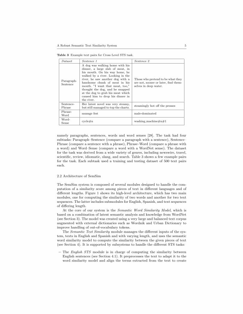
namely paragraphs, sentences, words and word senses [28]. The task had foursubtasks: Paragraph–Sentence (compare a paragraph with a sentence), Sentence–Phrase (compare a sentence with a phrase), Phrase–Word (compare a phrase witha word) and Word–Sense (compare a word with a WordNet sense). The datasetfor the task was derived from a wide variety of genres, including newswire, travel,scientific, review, idiomatic, slang, and search. Table 3 shows a few example pairsfor the task. Each subtask used a training and testing dataset of 500 text pairseach.

2.2 Architecture of SemSim

The SemSim system is composed of several modules designed to handle the com-putation of a similarity score among pieces of text in di↵erent languages and ofdi↵erent lengths. Figure 1 shows its high-level architecture, which has two mainmodules, one for computing the similarity of two words and another for two textsequences. The latter includes submodules for English, Spanish, and text sequencesof di↵ering length.

At the core of our system is the Semantic Word Similarity Model, which isbased on a combination of latent semantic analysis and knowledge from WordNet(see Section 3). The model was created using a very large and balanced text corpusaugmented with external dictionaries such as Wordnik and Urban Dictionary toimprove handling of out-of-vocabulary tokens.

The Semantic Text Similarity module manages the di↵erent inputs of the sys-tem, texts in English and Spanish and with varying length, and uses the semanticword similarity model to compute the similarity between the given pieces of text(see Section 4). It is supported by subsystems to handle the di↵erent STS tasks:

– The English STS module is in charge of computing the similarity betweenEnglish sentences (see Section 4.1). It preprocesses the text to adapt it to theword similarity model and align the terms extracted from the text to create


Fig. 1 High-level architecture of the SemSim system with the main modules.

a term alignment score. Then, it uses di↵erent supervised and unsupervisedmodels to compute the similarity score.

– The Spanish STS module computes the similarity between Spanish sentences(see Section 4.2). It makes use of an external statistical machine translation [7]software (Google Translate) to translate the sentences to English. Then, itenriches the translations by considering the possible multiple translations ofeach word. Finally, it uses the English STS module to compute the similaritybetween the translated sentences and combine the results obtained.

– The Cross-Level STS module is used to produce the similarity between text se-quences of varying lengths, such as words, senses, and phrases (see Section 4.3).It combines the features obtained by the English STS module with features ex-tracted from external dictionaries and Web search engines.

In the following sections we detail the previous modules and in Section 5 weshow the results obtained by SemSim at the di↵erent SemEval competitions.

3 Semantic Word Similarity Model

Our word similarity model was originally developed for the Graph of Relationsproject [52] which maps informal queries with English words and phrases for anRDF linked data collection into a SPARQL query. For this, we wanted a similarity


metric in which only the semantics of a word is considered and not its lexicalcategory. For example, the verb “marry” should be semantically similar to thenoun “wife”. Another desiderata was that the metric should give highest scoresand lowest scores in its range to similar and non-similar words, respectively. In thissection, we describe how we constructed the model by combining latent semanticanalysis (LSA) and WordNet knowledge and how we handled out-of-vocabularywords.

3.1 LSA Word Similarity

LSA word similarity relies on the distributional hypothesis that the words occur-ring in similar contexts tend to have similar meanings [25]. Thus, evidence forword similarity can be computed from a statistical analysis of a large text corpus.A good overview of the techniques for building distributional semantic models isgiven in [32], which also discusses their parameters and evaluation.

Corpus Selection and Processing. A very large and balanced text corpus is requiredto produce reliable word co-occurrence statistics. After experimenting with severalcorpus choices including Wikipedia, Project Gutenberg e-Books [26], ukWaC [5],Reuters News stories [46], and LDC Gigawords, we selected the Web corpus fromthe Stanford WebBase project [50]. We used the February 2007 crawl, which isone of the largest collections and contains 100 million web pages from more than50,000 websites. The WebBase project did an excellent job in extracting textualcontent from HTML tags but still o↵ers abundant text duplications, truncatedtext, non-English text and strange characters. We processed the collection to re-move undesired sections and produce high quality English paragraphs. Paragraphboundaries were detected using heuristic rules and only paragraphs with at leasttwo hundred characters were retained. We eliminated non-English text by checkingthe first twenty words of a paragraph to see if they were valid English words. Weused the percentage of punctuation characters in a paragraph as a simple check fortypical text. Duplicate paragraphs were recognized using a hash table and elimi-nated. This process produced a three billion word corpus of good quality English,which is available at [20].

Word Co-Occurrence Generation. We performed part of speech (POS) taggingand lemmatization on the WebBase corpus using the Stanford POS tagger [51].Word/term co-occurrences were counted in a moving window of a fixed size thatscanned the entire corpus4. We generated two co-occurrence models using windowsizes ±1 and ±45 because we observed di↵erent natures of the models. ±1 windowproduces a context similar to the dependency context used in [34]. It provides amore precise context, but only works for comparing words within the same POScategory. In contrast, a context window of ±4 words allows us to compute semanticsimilarity between words with di↵erent POS tags.

4 We used a stop-word list consisting of only the articles “a”, “an” and “the” to excludewords from the window. All remaining words were replaced by their POS-tagged lemmas.

5 Notice that ±4 includes all words up to ±4 and so it includes words at distances ±1, ±2,±3, and ±4.


A DT passenger NN plane NN has VBZ crashed VBN shortly RB after IN taking VBGo↵ RP from IN Kyrgyzstan NNP ’s POS capital NN , , Bishkek NNP , , killing VBG a DTlarge JJ number NN of IN those DT on IN board NN . .

Fig. 2 An example of a POS-tagged sentence.

Our experience has led us to conclusion that the ±1 window does an e↵ectivejob of capturing relations, given a good-sized corpus. A ±1 window in our con-text often represents a syntax relation between open-class words. Although longdistance relations can not be captured by this small window, this same relationcan also appear as ±1 relation. For example, consider the sentence “Who didthe daughter of President Clinton marry?”. The long distance relation “daughtermarry” can appear in another sentence “The married daughter has never beenable to see her parent again”. Therefore, statistically, a ±1 window can capturemany of the relations the longer window can capture. While the relations capturedby ±1 window can be wrong, the state-of-the-art statistical dependency parserscan produce errors, too.

Our word co-occurrence models were based on a predefined vocabulary of about22,000 common English words and noun phrases. The 22,000 common Englishwords and noun phrases are based on the online English Dictionary 3ESL, whichis part of the Project 12 Dicts6. We manullay exclude proper nouns from the 3ESLbecause there are not many of them and they are all ranked at the top places sinceproper nouns start with an uppercase letter. WordNet is used to assign part ofspeech tags to the words in the vocabulary because statistical POS parsers cangenerate incorrect POS tags to words. We also added more than 2,000 verb phrasesextracted from WordNet. The final dimensions of our word co-occurrence matricesare 29,000 ⇥ 29,000 when words are POS tagged. Our vocabulary includes onlyopen-class words (i.e., nouns, verbs, adjectives and adverbs). There are no propernouns (as identified by [51]) in the vocabulary with the only exception of an exploitlist of country names.

We use a small example sentence, “A passenger plane has crashed shortly aftertaking o↵ from Kyrgyzstan’s capital, Bishkek, killing a large number of those onboard.”, to illustrate how we generate the word co-occurrence models.

The corresponding POS tagging result from the Stanford POS tagger is shownin Figure 2. Since we only consider open-class words, our vocabulary for this smallexample will only contains 10 POS-tagged words in alphabetical order: board NN,capital NN, crash VB, kill VB, large JJ, number NN, passenger NN, plane NN,shortly RB and take VB. The resulting co-occurrence counts for the context win-dows of size ±1 and ±4 are shown in Table 4 and Table 5, respectively.

Stop words are ignored and do not occupy a place in the context window.For example, in Table 4 there is one co-occurrence count between “kill VB” and“large JJ” in the ±1 context window although there is an article “a DT” betweenthem. Other close-class words still occupy places in the context window althoughwe do not need to count co-occurrences when they are involved since they arenot in our vocabulary. For example, the co-occurrences count is zero between“shortly RB” and “take VB” in Table 4 since they are separated by “after IN”that is not a stop word. The reasons we only choose three articles as stop wordsare (1) they have high frequency in text; (2) they have few meanings; (3) we want

6 http://wordlist.aspell.net/12dicts-readme


Table 4 The word co-occurrence counts using ±1 context window for the sentence in Figure 2.

word POS # 1 2 3 4 5 6 7 8 9 10board NN 1 0 0 0 0 0 0 0 0 0 0capital NN 2 0 0 0 0 0 0 0 0 0 0crash VB 3 0 0 0 0 0 0 0 0 1 0kill VB 4 0 0 0 0 1 0 0 0 0 0large JJ 5 0 0 0 1 0 1 0 0 0 0number NN 6 0 0 0 0 1 0 0 0 0 0passenger NN 7 0 0 0 0 0 0 0 1 0 0plane NN 8 0 0 0 0 0 0 1 0 0 0shortly RB 9 0 0 1 0 0 0 0 0 0 0take VB 10 0 0 0 0 0 0 0 0 0 0

Table 5 The word co-occurrence counts using ±4 context window for the sentence in Figure 2.

word POS # 1 2 3 4 5 6 7 8 9 10board NN 1 0 0 0 0 0 1 0 0 0 0capital NN 2 0 0 0 1 0 0 0 0 0 0crash VB 3 0 0 0 0 0 0 1 1 1 1kill VB 4 0 1 0 0 1 1 0 0 0 0large JJ 5 0 0 0 1 0 1 0 0 0 0number NN 6 1 0 0 1 1 0 0 0 0 0passenger NN 7 0 0 1 0 0 0 0 1 1 0plane NN 8 0 0 1 0 0 0 1 0 1 0shortly RB 9 0 0 1 0 0 0 1 1 0 1take VB 10 0 0 1 0 0 0 0 0 1 0

to keep a small number of stop words for ±1 window since close-class words canoften isolate unrelated open-class words; and (4) we want to capture the relationin the pattern “verb + the (a, an) + noun” that frequently appear in text for ±1window, e.g., “know the person”.

SVD Transformation. Singular value decomposition (SVD) has been found to bee↵ective in improving word similarity measures [31]. SVD is typically applied toa word by document matrix, yielding the familiar LSA technique. In our case weapply it to our word by context word matrix. In literature, this variation of LSAis sometimes called HAL (Hyperspace Analog to Language) [9].

Before performing SVD, we transform the raw word co-occurrence count fij

toits log frequency log(f

ij

+1). We select the 300 largest singular values and reducethe 29K word vectors to 300 dimensions. The LSA similarity between two words isdefined as the cosine similarity of their corresponding word vectors after the SVDtransformation.

LSA Similarity Examples. Table 6 shows ten examples obtained using LSA simi-larity. Examples 1 to 6 show that the metric is good at di↵erentiating similar fromnon-similar word pairs. Examples 7 and 8 show that the ±4 model can detect se-mantically similar words even with di↵erent POS while the ±1 model yields muchworse performance. Examples 9 and 10 show that highly related but not substi-tutable words can also have a strong similarity, but the ±1 model has a betterperformance in discriminating them. We call the ±1 model concept similarity andthe ±4 model relation similarity, respectively, since the ±1 model performs best


Table 6 Ten examples from the LSA similarity model.

# Word Pair ±4 model ±1 model

1 doctor NN, physician NN 0.775 0.726

2 car NN, vehicle NN 0.748 0.802

3 person NN, car NN 0.038 0.024

4 car NN, country NN 0.000 0.016

5 person NN, country NN 0.031 0.069

6 child NN, marry VB 0.098 0.000

7 wife NN, marry VB 0.548 0.274

8 author NN, write VB 0.364 0.128

9 doctor NN, hospital NN 0.473 0.347

10 car NN, driver NN 0.497 0.281

on nouns and the ±4 model on relational phrases, regardless of their structure(e.g., “married to” and “is the wife of”).

3.2 Evaluation

TOEFL Synonym Evaluation. We evaluated the ±1 and ±4 models on the well-known 80 TOEFL synonym test questions. The ±1 and ±4 models correctly an-swered 73 and 76 questions, respectively. One question was not answerable becausethe question word, “halfheartedly”, is not in our vocabulary. If we exclude thisquestion, ±1 achieves an accuracy of 92.4% and ±4 achieves 96.2%. It is worthmentioning that this outstanding performance is obtained without testing on theTOEFL synonym questions beforehand.

According to ACL web page on state-of-the-art performance to TOEFL Syn-onym Questions,7 our result is second-to-best among all corpus-based approaches.The best performance was achieved by Bullinaria and Levy with a perfect accu-racy but it was the result of directly tuning their model on the 80 questions. Itis interesting that our models can perform so well, especially when our approachis much simpler than Bullinaria and Levy’s approach [8] or Rapp’s approach [44].There are several di↵errences between our system and exiting approaches. First,we used a three-billion word corpus with high quality, which is larger than cor-pora used by Bullinaria and Levy (two-billion) or Rapp (100 million). Second, weperformed POS tagging and lemmatization on the corpus. Third, our vocabularyincludes only open-class or content words.

WordSimilarity-353 Evaluation. WordSim353 is another dataset that is often usedto evaluate word similarity measures [17]. It contains 353 word pairs, each of whichis scored by 13 to 16 human subjects on a scale from 0 to 10. However, due tothe limited size of the vocabulary that we used, some words in the WordSim353dataset (e.g., “Arafat”) are outside of our vocabulary. Therefore, we chose to usea subset of WordSimilarity353 that had been used to evaluate a state-of-the-artword similarity measure PMI

max

[23] because both share the same 22,000 commonEnglish words as their vocabulary. This subset contains 289 word pairs. The evalu-ation result, including both the Pearson correlation and Spearman rank correlation

7 http://goo.gl/VtiObt


Table 7 Evaluating our LSA ±4 model on 289 pairs in WordSim353 dataset and comparingthe results with the state-of-the-art word similarity measure PMI

max

[23].

Pearson SpearmanPMI

max

0.625 0.666LSA ±4 model 0.642 0.727

Table 8 Comparison of our LSA models to the Word2Vec model [41] on the 80 TOEFLsynonym questions.

±1 model ±4 model Word2VecCorrectly Answered 73 76 67Accuracy 92.4% 96.2% 84.8%Out-Of-Vocabulary Words halfheartedly halfheartedly tranquillity

coe�cients, is shown in Table 7. Since WordSim353 is a dataset more suitable forevaluating semantic relatedness than semantic similarity, we only evaluate the ±4model on it. The LSA ±4 model performed better than PMI

max

in both Pearsonand Spearman correlation.

If the 289 pairs could be thought as a representative sample of the 353 pairsand if we could thereby compare our result with the state-of-the-art evaluations onWordSimilarity-353 [1], the Pearson correlation of 0.642 produced by our model isranked as the second to best among all state-of-the-art approaches.

Comparison with Word2Vec. For the final evaluation, we also compared our LSAmodels to the Word2Vec [41] word embedding model on the TOEFL synonymquestions. We used the pre-trained model also published by Mikolov et al. [41],which was trained on a collection of more than 100 billion words from GoogleNews. The model contains 300-dimensional vectors, which has the same dimensionas our models. One question word “tranquillity” is not in the pre-trained model’svocabulary8. Therefore, both sides have one question not answerable. The resultsof both systems are shown in Table 8. Our LSA models’ performance is significantlybetter than the Word2Vec model, at a 95% confidence level using the BinomialExact Test.

3.3 Combining with WordNet Knowledge

Statistical word similarity measures have limitations. Related words can have sim-ilarity scores only as high as their context overlap, as illustrated by “doctor” and“hospital” in Table 6. Also, word similarity is typically low for synonyms havingmany word senses since information about di↵erent senses are mixed together [23].We can reduce the above issues by using additional information from WordNet.

Boosting LSA similarity using WordNet. We increase the similarity between twowords if any relation in the following eight categories hold:

1. They are in the same WordNet synset.2. One word is the direct hypernym of the other.3. One word is the two-link indirect hypernym of the other.

8 The spelling tranquillity dominated tranquility prior to 1980, but is now much less common.


4. One adjective has a direct similar to relation with the other.5. One adjective has a two-link indirect similar to relation with the other.6. One word is a derivationally related form of the other.7. One word is the head of the gloss of the other or its direct hypernym or one of

its direct hyponyms.8. One word appears frequently in the glosses of the other and its direct hypernym.

Notice that categories 1-6 are based on linguistic properties whereas categories7-8 are more heuristic. We use the algorithm described in [12] to find a word glossheader.9

We define a word’s “significant senses” to deal with the problem of WordNettrivial senses. The word “year”, for example, has a sense “a body of students whograduate together” which makes it a synonym of the word “class”. This causesproblems because this is not the most significant sense of the word “year”. A senseis significant if any of the following conditions are met: (i) it is the first sense; (ii)its WordNet frequency count is at least five; or (iii) its word form appears first inits synset’s word form list and it has a WordNet sense number less than eight.

We require a minimum LSA similarity of 0.1 between the two words to filterout noisy data when extracting relations in the eight WordNet categories becausesome relations in the categories are not semantically similar. One is because ourheuristic definition of ”significant sense” sometimes can include trivial sense of aword, therefore, noise. The second reason is that the derivational form of a wordis not necessarily semantically similar to the word. The third reason is that thecategory 7 and 8 can produce incorrect results sometimes.

We adopt the concept of path distance from [33] and assign path distance ofzero to the category 1, path distance of one to the categories 2, 4, and 6, and pathdistance of two to categories 3, 5, 7, and 8. Categories 1-6 follow the definitionin Li et al. but 7 and 8 are actually not related to path distance. However, inorder to have a uniform equation to compute the score, we assume that thesetwo categories can be boosted by a score equivalent to path length of 2, which islongest path distance in our eight categories. The new similarity between wordsx and y is computed by combining the LSA similarity and WordNet relations asshown in the following equation,

sim�(x, y) = min(1, simLSA

(x, y) + 0.5e�↵D(x,y)) (1)

where D(x, y) is the minimal path distance between x and y. Using e

�↵D(x,y) totransform simple shortest path length has been demonstrated to be very e↵ectiveby [33]. The parameter ↵ is set to 0.25, following their experimental results.

Dealing with words of many senses. For a word w with many WordNet senses(currently ten or more), we use its synonyms with fewer senses (at most one thirdof that of w) as its substitutions in computing similarity with another word. LetS

x

and S

y

be the set of all such substitutions of the words x and y respectively.The new similarity is obtained using Equation 2.

sim(x, y) = max( maxs

x

2S

x

[{x}sim�(s

x

, y),

maxs

y

2S

y

[{y}sim�(x, s

y

)) (2)

9 For example, the gloss of the first sense of “doctor” in WordNet is “a licensed medicalpractitioner”. The gloss head of “doctor” is therefore “practitioner”.


Table 9 Fraction of OOV words generated by Stanford POS tagger for a sample of 500sentences per dataset.

dataset Noun Adjective Verb Adverb

MSRvid 0.09 0.27 0.04 0.00

MSRpar 0.39 0.37 0.01 0.03

SMT 0.18 0.19 0.03 0.05

headlines 0.40 0.44 0.02 0.00

OnWn 0.08 0.10 0.01 0.1

Finally, notice that some of the design choices in this section were made byintuition, observations, and a small number of sampled and manually checkedexperiments. Therefore some of the choices/parameters have a heuristic natureand may be suboptimal. The reason why we do so is because many parametersor choices in defining eight categories, “significant senses”, and similarity func-tions are intertwined. Due to the number of them, justifying every design choicerequires many detailed experiments, which we cannot o↵er in this paper. TheLSA+WordNet model was originally developed for Graph of Relation project or aschema-agnostic graph query system, as we pointed earlier in the paper. The ad-vantage of LSA+WordNet model with these intuitive and pragmatic design choicesover the pure LSA model has been demonstrated in the experiments on the graphquery system [19]. An online demonstration of a similar model developed for theGOR project is available [53].

3.4 Out-of-Vocabulary Words

Our word similarity model is restricted by the size of its predefined vocabulary (setof (token, part�of�speech) tuples). Any word absent from this set is called an out-of-vocabulary (OOV) word. For these, we can only rely on their lexical features likecharacter unigrams, bigrams, etc. While the vocabulary is large enough to handlemost of the commonly used words, for some domains OOV words can become asignificant set. Table 9 shows the fraction of OOV words in a random sample of500 sentences from the STS datasets when Stanford POS tagger was used. Table10 gives some example OOV words.

The most common type of OOV words are names (proper nouns) and theiradjective forms. For example, the noun “Palestine” and its adjective form “Pales-tinian”. This is apparent from Table 9 where some datasets have high OOV nounsand adjectives due to the nature of their domain. For instance, MSRpar andheadlines are derived from newswire and hence contain a large number of namesof people, places, and organizations. Other OOV words include lexical variants(“summarise” vs “summarize”), incorrectly spelled words (“nterprise”), hyphen-ated words (multi-words), rare morphological forms, numbers, and time expres-sions. Since our vocabulary is actually a set of (token, part� of � speech) tuples,incorrect POS tagging also contributes to OOV words.

Since OOV words do not have a representation in our word similarity model,we cannot compare them with any other word. One approach to alleviate thisis to include popular classes of OOV words like names into our vocabulary. Forhighly focused domains like newswire or cybersecurity, this would be a reasonable


Table 10 Examples of OOV words.

POS example OOV words

Noun gadhafi, spain, jihad, nterprise, jerry, biotechnology, health-care

Adjective six-day, 20-member, palestinian, islamic, coptic, yemeni

Verb self-immolate, unseal, apologise, pontificate, summarise, plough

Adverb faster, domestically, minutely, shrilly, thirdly, amorously

and useful approach. For instance, it would be useful to know that “Mozilla Fire-fox” is more similar to “Google Chrome” than “Adobe Photoshop”. However, forgeneric models, this would vastly increase the vocabulary size and would requirelarge amounts of high quality training data. Also, in many cases, disambiguatingnamed entities would be better than computing distributional similarity scores.For instance, while “Barack Obama” is somewhat similar to “Joe Biden” in thatthey both are politicians and democrats, in many cases it would be unacceptableto have them as substitutable words. Another approach is to handle these OOVterms separately by using a di↵erent representation and similarity function.

Lexical OOV Word Similarity. We built a simple wrapper to handle OOV wordslike proper nouns, numbers and pronouns. We handle pronouns heuristically andcheck for string equivalence for numbers. For any other open class OOV word,we use simple character bigram representations. For example, the name “Barack”would be represented by the set of bigrams {‘ba’,‘ar’,‘ra’,‘ac’,‘ck’}. To comparea pair of words, we compute the Jaccard coe�cient of their bigrams and thenthreshold the value to disambiguate the word pair.10

Semantic OOV Word Similarity. Lexical features work only for word disambigua-tion and make little sense when computing semantic similarity. While many OOVwords come from proper nouns, for which disambiguation works well, languagescontinue to grow and add new words into their vocabulary. To simply use lexicalfeatures for OOV words would restrict the model’s ability to adapt to a growinglanguage. For example, the word “google” has become synonymous with “search”and is often used as a verb. Also, as usage of social media and micro-blogginggrows, new slang, informal words, abbreviations come into existence and becomea part of common discourse.

As these words are relatively new, including them in our distributional wordsimilarity model might yield poor results, since they lack su�cient training data.To address this, we instead represent them by their dictionary features like defi-nitions, usage examples, or synonyms retrieved from external dictionaries. Giventhis representation, we can then compute the similarity as the sentence similarityof their definitions [24,29]. To retrieve reliable definitions, we need good sourcesof dictionaries with vast vocabulary and accurate definitions. We describe twodictionary resources that we used for our system.

Wordnik [13] is an online dictionary and thesaurus resource that includes severaldictionaries like the American Heritage dictionary, WordNet, and Wikitionary. Itexposes a REST API to query their dictionary, although the daily usage limits

10 Our current system uses a threshold value of 0.8, which we observed to produce goodresults.


for the API adds a bottleneck to our system. Wordnik has a large set of uniquewords and their corresponding definitions for di↵erent senses, examples, synonyms,and related words. For our system, we use the top definition retrieved from theAmerican Heritage dictionary and Wikitionary as context for an OOV word. Wetake the average of the sentence similarity scores between these two dictionariesand use it as our OOV word similarity score. Usually the most popular sense fora word is Wordnik’s first definition. In some cases, the popular sense was di↵erentbetween the American Heritage Dictionary and Wikitionary which added noise.Even with its vast vocabulary, several slang words and phrases were found to beabsent in Wordnik. For this, we used content from the Urban Dictionary.

Urban Dictionary [54] is a crowd-sourced dictionary source that has a largecollection of words and definitions added by users. This makes it a very valuableresource for contemporary slang words and phrases. Existing definitions are alsosubject to voting by the users. While this helps accurate definitions achieve ahigher rank, popularity does not necessarily imply accuracy. We experimentedwith Urban Dictionary to retrieve word definitions for the Word2Sense subtask asdescribed in Section 4.3.2. Due to the crowd-sourced nature of the resource, it isinherently noisy with sometimes verbose or inaccurate definitions. For instance, thetop definition of the word “Programmer” is “An organism capable of convertingca↵eine into code” whereas the more useful definition “An individual skilled atwriting software code” is ranked fourth.

4 Semantic Textual Similarity

In this section, we describe the various algorithms developed for the *SEM 2013and SemEval-2014 tasks on Semantic Textual Similarity.

4.1 English STS

We developed two systems for the English STS task, which are based on theword similarity model explained in Section 3. The first system, PairingWords,uses a simple term alignment algorithm. The second system combines these scoreswith additional features for the given training data to train supervised models.We apply two di↵erent approaches to these supervised systems: an approach thatuses generic models trained on all features and data (Galactus/Hulk) and an ap-proach that uses specialized models trained on domain specific features and data(Saiyan/SuperSaiyan).

Preprocessing. We initially process the text by performing tokenization, lemmati-zation and part of speech tagging, as required by our word similarity model. Weuse open-source tools from Stanford coreNLP [16] and NLTK [6] for these tasks.Abbreviations are expanded by using a complied list of commonly used abbrevia-tions for countries, North American states, measurement units, etc.


Term Alignment. Given two text sequences, we first represent them as two sets ofrelevant keywords, S1 and S2. Then, for a given term t 2 S1, we find its counterpartin the set S2 using the function g1 as defined by

g1(t) = argmax

t

02S2

sim(t, t0) t 2 S1 (3)

where sim(t, t0) is the semantic word similarity between terms t and t

0.

Similarly, we define the alignment function g2 for the other direction as:

g2(t) = argmax

t

02S1

sim(t, t0) t 2 S2 (4)

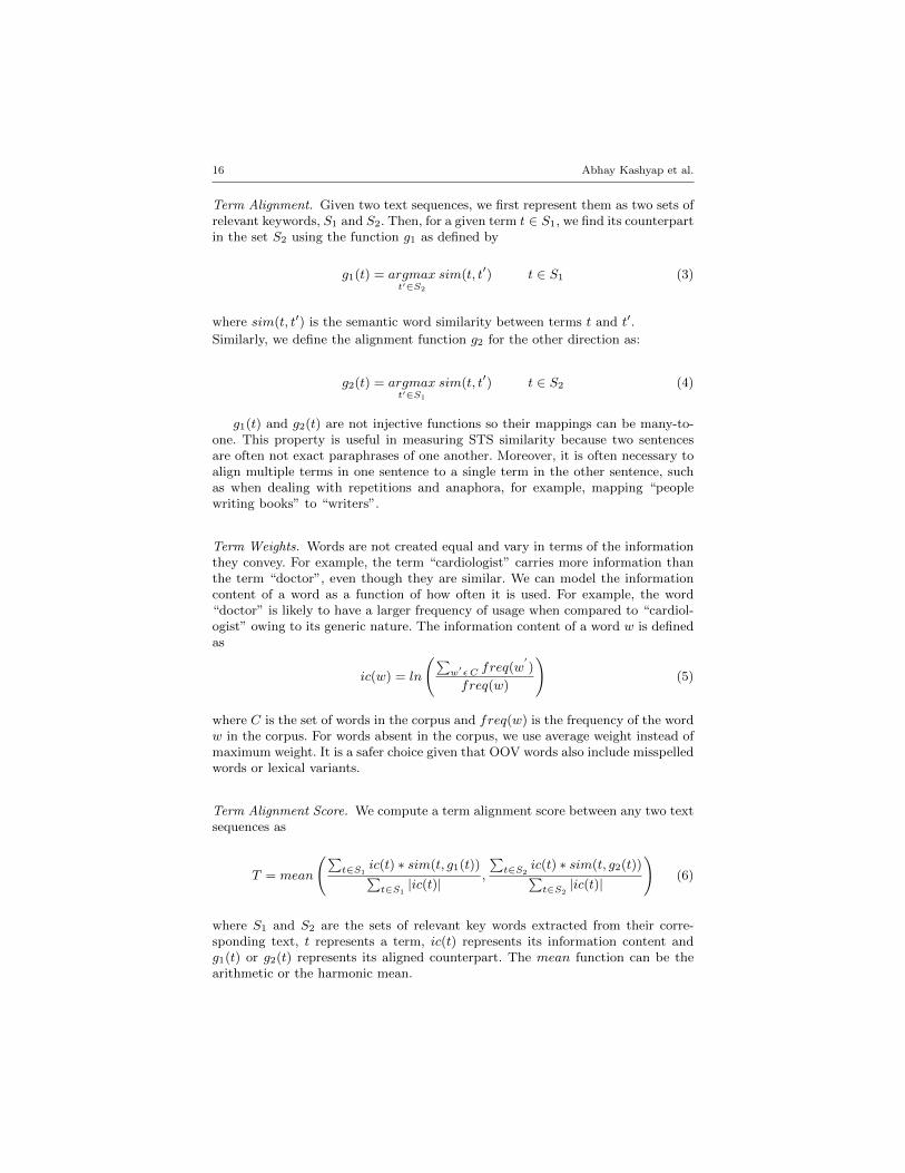
g1(t) and g2(t) are not injective functions so their mappings can be many-to-one. This property is useful in measuring STS similarity because two sentencesare often not exact paraphrases of one another. Moreover, it is often necessary toalign multiple terms in one sentence to a single term in the other sentence, suchas when dealing with repetitions and anaphora, for example, mapping “peoplewriting books” to “writers”.

Term Weights. Words are not created equal and vary in terms of the informationthey convey. For example, the term “cardiologist” carries more information thanthe term “doctor”, even though they are similar. We can model the informationcontent of a word as a function of how often it is used. For example, the word“doctor” is likely to have a larger frequency of usage when compared to “cardiol-ogist” owing to its generic nature. The information content of a word w is definedas

ic(w) = ln

Pw

0✏C

freq(w0)

freq(w)

!(5)

where C is the set of words in the corpus and freq(w) is the frequency of the wordw in the corpus. For words absent in the corpus, we use average weight instead ofmaximum weight. It is a safer choice given that OOV words also include misspelledwords or lexical variants.

Term Alignment Score. We compute a term alignment score between any two textsequences as

T = mean

Pt2S1

ic(t) ⇤ sim(t, g1(t))Pt2S1

|ic(t)| ,

Pt2S2

ic(t) ⇤ sim(t, g2(t))Pt2S2

|ic(t)|

!(6)

where S1 and S2 are the sets of relevant key words extracted from their corre-sponding text, t represents a term, ic(t) represents its information content andg1(t) or g2(t) represents its aligned counterpart. The mean function can be thearithmetic or the harmonic mean.


4.1.1 PairingWords: Align and Penalize

We hypothesize that STS similarity between two text sequences can be computedusing

STS = T � P

0 � P

00 (7)

where T is the term alignment score, P 0 is the penalty for bad alignments, andP

00 is the penalty for syntactic contradictions led by the alignments. However P 00

had not been fully implemented and is not used in our STS systems. We show ithere just for completeness.

We compute T from Equation 6 where the mean function represents the arith-metic mean. The similarity function sim

0(t, t0) is a simple lexical OOV word simi-larity back-o↵ (see Section 3.4) over sim(x, y) in Equation 2 that uses the relationsimilarity.

We currently treat two kinds of alignments as “bad”, as described in Equa-tion 8. The similarity threshold ✓ in defining A

i

should be set to a low score, suchas 0.05. For the set B

i

, we have an additional restriction that neither of the sen-tences has the form of a negation. In defining B

i

, we used a collection of antonymsextracted from WordNet [43]. Antonym pairs are a special case of disjoint sets.The terms “piano” and “violin” are also disjoint but they are not antonyms. Inorder to broaden the set B

i

we will need to develop a model that can determinewhen two terms belong to disjoint sets.

A

i

=�ht, g

i

(t)i |t 2 S

i

^ sim

0(t, gi

(t)) < ✓

B

i

= {ht, gi

(t)i |t 2 S

i

^ t is an antonymof gi

(t)}i 2 {1, 2} (8)

We show how we compute P

0 in the following:

P

A

i

=

Pht,g

i

(t)i2A

i

(sim0(t, gi

(t)) + w

f

(t) · wp

(t))

2 · |Si

|

P

B

i

=

Pht,g

i

(t)i2B

i

(sim0(t, gi

(t)) + 0.5)

2 · |Si

|P

0 = P

A

1 + P

B

1 + P

A

2 + P

B

2 (9)

w

f

(t) and w

p

(t) terms are two weighting functions on the term t. wf

(t) inverselyweights the log frequency of term t and w

p

(t) weights t by its part of speech tag,assigning 1.0 to verbs, nouns, pronouns and numbers, and 0.5 to terms with otherPOS tags.

4.1.2 Galactus/Hulk and Saiyan/Supersaiyan: Supervised systems

The PairingWords system is completely unsupervised. To leverage the availabil-ity of training data, we combine the scores from PairingWords with additionalfeatures and learn supervised models using support vector regression (SVR). Weused LIBSVM [10] to learn an epsilon SVR with a radial basis kernel and ran agrid search provided by [48] to find the optimal values for the parameters cost,gamma and epsilon. We developed two systems for the *SEM 2013 STS task,Galactus and Saiyan, which we used as a basis for the two systems developed forthe SemEval-2014 STS task, Hulk and SuperSaiyan.


Galactus and Saiyan: 2013 STS task. We used NLTK’s [6] default Penn Treebankbased tagger to tokenize and POS tag the given text. We also used regular ex-pressions to detect, extract, and normalize numbers, date, and time, and removedabout 80 stopwords. Instead of representing the given text as a set of relevantkeywords, we expanded this representation to include bigrams, trigrams, and skip-bigrams, a special form of bigrams which allow for arbitrary distance between twotokens. Similarities between bigrams and trigrams were computed as the averageof the similarities of its constituent terms. For example, for the bigrams “mouseate” and “rat gobbled”, the similarity score is the average of the similarity scoresbetween the words “mouse” and “rat” and the words “ate” and “gobbled”. Termweights for bigrams and trigrams were computed similarly.

The aligning function is similar to Equation 3 but is an exclusive alignmentthat implies a term can only be paired with one term in the other sentence. Thismakes the alignment direction independent and a one-one mapping. We use refinedversions of Google ngram frequencies [39], from [37] and [48], to get the informationcontent of the words. The similarity score is computed by Equation 6 where themean function represents the Harmonic mean. We used several word similarityfunctions in addition to our word similarity model. Our baseline similarity functionwas an exact string match which assigned a score of 1 if two tokens contained thesame sequence of characters and 0 otherwise. We also used NLTK’s library tocompute WordNet based similarity measures such as Path Distance Similarity,Wu-Palmer similarity [55], and Lin similarity [35]. For Lin similarity, the Semcorcorpus was used for the information content of words. Our word similarity wasused in concept, relation, and mixed mode (concept for nouns, relation otherwise).To handle OOV words, we used the lexical OOV word similarity as described inSection 3.4.

We computed contrast features using three di↵erent lists of antonym pairs [43].We used a large list containing 3.5 million antonym pairs, a list of about 22,000antonym pairs from WordNet and a list of 50,000 pairs of words with their degreeof contrast. The contrast score is computed using Equation 6 but the sim(t, t0)contains negative values to indicate contrast scores.

We constructed 52 features from di↵erent combinations of similarity metrics,their parameters, ngram types (unigram, bigram, trigram and skip-bigram), andngram weights (equal weight vs. information content) for all sentence pairs in thetraining data:

– We used scores from the align-and-penalize approach directly as a feature.– Using exact string match over di↵erent ngram types and weights, we extracted

eight features (4 ⇤ 2). We also developed four additional features (2 ⇤ 2) by in-cluding stopwords in bigrams and trigrams, motivated by the nature of MSRviddataset.

– We used the LSA-boosted similarity metric in three modes: concept similarity(for nouns), relation similarity (for verbs, adjectives and adverbs), and mixedmode. A total of 24 features were extracted (4 ⇤ 2 ⇤ 3).

– For WordNet-based similarity measures, we used uniform weights for Path andWu-Palmer similarity and used the information content of words (derived fromthe Semcor corpus) for Lin similarity. Skip bigrams were ignored and a totalof nine features were produced (3 ⇤ 3).


Table 11 Fraction of OOV words generated by NLTK’s Penn Treebank POS tagger.

dataset (#sentences) Noun Adjective Verb Adverb

MSRpar (1500) 0.47 0.25 0.10 0.13

SMT (1592) 0.26 0.12 0.09 0.10

headlines (750) 0.43 0.41 0.13 0.27

OnWN (1311) 0.24 0.24 0.10 0.23

– Contrast scores used three di↵erent lists of antonym pairs. A total of six fea-tures were extracted using di↵erent weight values (3 ⇤ 2).

The Galactus system was trained on all of the STS 2012 data and used the fullset of 52 features. The Saiyan system employed data-specific training and features.More specifically, the model for headlines was trained on 3000 sentence pairs fromMSRvid and MSRpar, SMT used 1500 sentence pairs from SMT europarl and SMTnews, while OnWN used only the 750 OnWN sentence pairs from last year. TheFnWN scores were directly used from the Align-and-Penalize approach. None ofthe models for Saiyan used contrast features and the model for SMT also ignoredsimilarity scores from exact string match metric.

Hulk and SuperSaiyan: 2014 STS task. We made a number of changes for the 2014tasks in an e↵ort to improve performance, including the following:

– We looked at the percentage of OOV words generated by NLTK (Table 11) andStanford coreNLP [16] (Table 9). Given the tagging inaccuracies by NLTK, weswitched to Stanford coreNLP for the 2014 tasks. Considering the sensitivityof some domains to names, we extracted named entities from the text alongwith normalized numbers, date and time expressions.

– While one-one alignment can reduce the number of bad alignments, it is notsuitable when comparing texts of di↵erent lengths. This was true in the caseof datasets like FrameNet-WordNet, which mapped small phrases with longersentences. We thus decided to revert to the direction-dependent, many-onemapping used by the PairingWords system.

– To address the high fraction of OOV words, the semantic OOV word similarityfunction as described in Section 3.4 was used.

– The large number of features used in 2013 gave marginally better results insome isolated cases but also introduced noise and increased training time. Thefeatures were largely correlated since they were derivatives of the basic termalignment with minor changes. Consequently, we decided to use only the scorefrom PairingWords and score computed using the semantic OOV word simi-larity.

In addition to these changes Galactus was renamed Hulk and trained on atotal of 3750 sentence pairs (1500 from MSRvid, 1500 from MSRpar and 750 fromheadlines). Datasets like SMT were excluded due to poor quality. Also, Saiyanwas renamed SuperSaiyan. For OnWN, we used 1361 sentence pairs from previousOnWN dataset. For Images, we used 1500 sentence pairs from MSRvid dataset.The others lacked any domain specific training data so we used a generic trainingdataset comprising 5111 sentence pairs from MSRvid, MSRpar, headlines andOnWN datasets.


Fig. 3 Our approach to compute the similarity between two Spanish sentences.

4.2 Spanish STS

Adapting our English STS system to handle Spanish similarity would require toselect a large and balanced Spanish text corpus and the use of a Spanish dic-tionary (such as the Multilingual Central Repository [18]). As a baseline for theSemEval-2014 Spanish subtask, we first considered translating the Spanish sen-tences to English and running the same systems explained for the English subtask(i.e., PairingWords and Hulk). The results obtained applying this approach to theprovided training data were promising (with a correlation of 0.777). So, insteadof adapting the systems to Spanish, we performed a preprocessing phase basedon the translation of the Spanish sentences (with some improvements) for thecompetition (see Figure 3).

Translating the sentences. To automatically translate sentences from Spanish toEnglish we used the Google Translate API,11 a free, multilingual machine trans-lation product by Google. It produces very accurate translations for Europeanlanguages by using statistical machine translation [7], where the translations aregenerated on the basis of statistical models derived from bilingual text corpora.Google used as part of this corpora 200 billion words from United Nations doc-uments that are typically published in all six o�cial UN languages, includingEnglish and Spanish.

In the experiments performed with the trial data, we manually evaluated thequality of the translations (one of the authors is a native Spanish speaker) andfound the overall translations to be very accurate. Some statistical anomalies werenoted that were due to incorrect translations because of the abundance of a specific

11 http://translate.google.com


word sense in the training set. On one hand, some homonym and polysemouswords are wrongly translated which is a common problem of machine translationsystems. For example, the Spanish sentence “Las costas o costa de un mar [...]”was translated to “Costs or the cost of a sea [...]”. The Spanish word costahas two di↵erent senses: “coast” (the shore of a sea or ocean) and “‘cost” (theproperty of having material worth). On the other hand, some words are translatedpreserving their semantics but with a slightly di↵erent meaning. For example, theSpanish sentence “Un cojın es una funda de tela [...]” was correctly translated to“A cushion is a fabric cover [...]”. However, the Spanish sentence “Una almohadaes un cojın en forma rectangular [...]” was translated to “A pillow is a rectangularpad [...]”.12

Dealing with Statistical Anomalies. The aforementioned problem of statistical ma-chine translation caused a slightly adverse e↵ect when computing the similarityof two English (translated from Spanish) sentences with the systems explained inSection 4.1. Therefore, we improved the direct translation approach by taking intoaccount the di↵erent possible translations for each word in a Spanish sentence. Forthat, we used Google Translate API to access all possible translations for everyword of the sentence along with a popularity value. For each Spanish sentence thesystem generates all its possible translations by combining the di↵erent possibletranslations of each word (in Figure 3 TS11, TS12...TS1n are the possible trans-lations for sentence SPASent1). For example, Figure 4 shows three of the Englishsentences generated for a given Spanish sentence from the trial data.

SPASent1: Las costas o costa de un mar, lago o extenso rıo es latierra a lo largo del borde de estos.

TS11: Costs or the cost of a sea, lake or wide river is theland along the edge of these.

TS12: Coasts or the coast of a sea, lake or wide river is theland along the edge of these.

TS13: Coasts or the coast of a sea, lake or wide river is theland along the border of these.

...

Fig. 4 Three of the English translations for the Spanish sentence SPASent1.

To control the combinatorial explosion of this step, we limited the maximumnumber of generated sentences for each Spanish sentence to 20 and only selectedwords with a popularity greater than 65. We arrived at the popularity thresholdthrough experimentation on every sentence in the trial data set. After this filtering,our input for the “news” and “Wikipedia” tests (see Section 2.1) went from 480and 324 pairs of sentences to 5756 and 1776 pairs, respectively.

Computing the Similarity Score. The next step was to apply the English STS sys-tem to the set of alternative translation sentence pairs to obtain similarity scores(see TS11vsTS21...TS1nvsTS2m in Figure 3). These were then combined to pro-duce the final similarity score for the original Spanish sentences. An intuitive way

12 Notice that both Spanish sentences used the term cojın that should be translated ascushion (the Spanish word for pad is almohadilla).


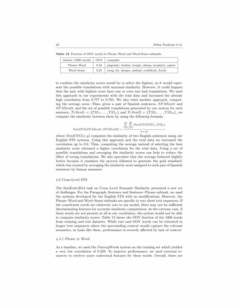
Table 12 Fraction of OOV words in Phrase–Word and Word-Sense subtasks.

dataset (1000 words) OOV examples

Phrase–Word 0.16 jingoistic, braless, bougie, skimp, neophyte, raptor

Word–Sense 0.25 swag, lol, cheapo, assload, cockblock, froofy

to combine the similarity scores would be to select the highest, as it would repre-sent the possible translations with maximal similarity. However, it could happenthat the pair with highest score have one or even two bad translations. We usedthis approach in our experiments with the trial data and increased the alreadyhigh correlation from 0.777 to 0.785. We also tried another approach, comput-ing the average score. Thus, given a pair of Spanish sentences, SPASent1 andSPASent2, and the set of possible translations generated by our system for eachsentence, TrSent1 = {TS11, . . . , TS1n} and TrSent2 = {TS21, . . . , TS2m}, wecompute the similarity between them by using the following formula:

SimSPA(SPASent1, SPASent2) =

nPi=1

mPj=1

SimENG(TS1i

, TS2j

)

n ⇤m

where SimENG(x, y) computes the similarity of two English sentences using ourEnglish STS systems. Using this approach and the trial data we increased thecorrelation up to 0.8. Thus, computing the average instead of selecting the bestsimilarity score obtained a higher correlation for the trial data. Using a set ofpossible translations and averaging the similarity scores can help to reduce thee↵ect of wrong translations. We also speculate that the average behaved slightlybetter because it emulates the process followed to generate the gold standard,which was created by averaging the similarity score assigned to each pair of Spanishsentences by human assessors.

4.3 Cross-Level STS

The SemEval-2014 task on Cross–Level Semantic Similarity presented a new setof challenges. For the Paragraph–Sentence and Sentence–Phrase subtask, we usedthe systems developed for the English STS with no modifications. However, thePhrase–Word and Word–Sense subtasks are specific to very short text sequences. Ifthe constituent words are relatively rare in our model, there may not be su�cientdiscriminating features for accurate similarity computation. In the extreme case, ifthese words are not present at all in our vocabulary, the system would not be ableto compute similarity scores. Table 12 shows the OOV fraction of the 1000 wordsfrom training and test datasets. While rare and OOV words can be tolerated inlonger text sequences where the surrounding context would capture the relevantsemantics, in tasks like these, performance is severely a↵ected by lack of context.

4.3.1 Phrase to Word

As a baseline, we used the PairingWords system on the training set which yieldeda very low correlation of 0.239. To improve performance, we used external re-sources to retrieve more contextual features for these words. Overall, there are


seven features: the baseline score from the PairingWords system, three dictionarybased features, and three web search based features.

Dictionary Features. In Section 3.4 we described the use of dictionary featuresas representation for OOV words. For this task, we extend it to all the words.To compare word and phrase, we retrieve a word’s definitions and examples fromWordnik and compare these with the phrase using our PairingWords system. Themaximum score when definitions and examples are compared with the phrase con-stitutes two features in the algorithm. The intuition behind taking the maximumis that the word sense which is most similar to the phrase is selected.

Following the 2014 task results, it was found that representing each phraseas a bag of words fared poorly for certain datasets, for example slang words andidioms. To address this, we added a third dictionary based feature based on thesimilarity of all Wordnik definitions of the phrase with all of the word’s definitionsusing our PairingWords system. This yielded a significant improvement over ourresults submitted in SemEval task as shown in Section 5.

Web Search Features. Dictionary features come with their own set of issues, asdescribed in Section 3.4. To overcome these shortcomings, we supplemented thesystem with Web search features. Since search engines provide a list of documentsranked by relevancy, an overlap between searches for the word, the phrase and acombination of the word and phrase, is evidence of similarity. This approach sup-plements our dictionary features by providing another way to recognize polysemouswords and phrases, e.g., that ’java’ can refer to co↵ee, an island, a programminglanguage, a Twitter handle, and many other things. It also addresses words andphrases that are at di↵erent levels of specificity. For example, ’object oriented pro-gramming language’ is a general concept and ’java object oriented programminglanguage’ is more specific. A word or phrase alone lacks any context that coulddiscriminate between meanings [42,45]. Including additional words or phrases ina search query provides context that supports comparing words and phrases withdi↵erent levels of specificity.

Given the set A and a word or phrase p

A

where p

A

2 A, a search on A willresult in a set of relevant documents D

A

. Given the set B and a word or phrase pB

where p

B

2 B, if we search on B, we will receive a set of relevant documents forB given by D

B

. Both searches will return what the engine calculates as relevantgiven A or B. So if we search on a new set C which includes A and B, such thatp

A

2 C and p

B

2 C then our new search result will be what the engine deemsrelevant, D

C

. If pA

is similar to p

B

and neither are polysemous, then D

A

, DB

andD

C

will overlap, shown in Figure 5(a). If either p

A

or p

B

is polysemous but notboth, then there may only be overlap between either A and C or B and C, shownin Figure 5(b). If both p

A

and p

B

are polysemous, then the three document setsmay not overlap, shown in Figure 5(c). In the case of a polysemous word or phrase,the overlapping likelihood is based on which meaning is considered most relevantby the search engine. For example, if p

A

is ’object oriented programming’ and p

B

is’java’, there is a higher likelihood that ’object oriented programming’ + ’java’, p

C

,will overlap with either p

A

or pB

if ’java’ as it relates to ’the programming language’is most relevant. However, if ’java’ as it relates to ’co↵ee’ is most relevant thenthe likelihood of overlap is low.

Specificity also a↵ects the likelihood of overlap. For example, even if the searchengine returns a document set that is relevant to the intended meaning of ’java’


or p

B

, the term is more specific than ’object oriented programming’ or p

A

andtherefore less likely to overlap. However since the combination of ’object orientedprogramming’ + ’java’ or p

C

acts as a link between p

A

and p

B

, the overlap betweenA , C and B , C could allow us to infer similarity between A and B or similarityspecifically between ’object oriented programming’ and ’java’.

(a) (b) (c)

(d)

Fig. 5 (a) Overlap between A, B, and C; (b) overlap between ’A and C’ or ’B and C’; (c) nooverlap between A, B and C; (d) overlap between ’A and C’ and ’B and C’.

We implemented this idea by comparing results of three search queries: theword, phrase, and the word and phrase together. We retrieved the top five resultsfor each search using the Bing Search API13 and indexed the resulting documentsets in Lucene [27] to obtain term frequencies for each search. For example, wecreated an index for the phrase ’spill the beans’, an index for the word ’confess’,and an index for ’spill the beans confess’. Using term frequency vectors for eachwe calculated the cosine similarity of the document sets. In addition, we alsocalculated the mean and minimum similarity among document sets. The similarityscores, the mean similarity, and minimum similarity were used as features, inaddition to the dictionary features, for the SVM regression model. We evaluatedhow our performance improved given our di↵erent sets of features. Table 19 showsthe cumulative e↵ect of adding these features.

4.3.2 Word to Sense

For the Word to Sense evaluation, our approach is similar to that described in theprevious section. However, we restrict ourselves to only dictionary features sinceusing Web search as a feature is not easily applicable when dealing with wordsenses. We will use an example word author#n and a WordNet sense Dante#n#1to explain the features extracted. We start by getting the word’s synonym set, W

i

,from WordNet. For the word author#n, W

i

comprises writer.n.01, generator.n.03and author.v.01. We then retrieve their corresponding set of definitions, D

i

. TheWordNet definition of writer.n.01, “writes (books or stories or articles or the like)

13 http://bing.com/developers/s/APIBasics.html


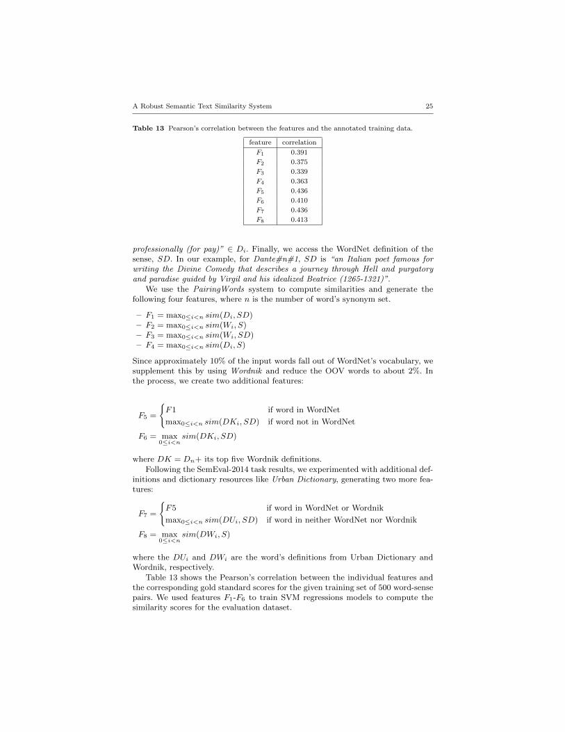
Table 13 Pearson’s correlation between the features and the annotated training data.

feature correlation

F1 0.391

F2 0.375

F3 0.339

F4 0.363

F5 0.436

F6 0.410

F7 0.436

F8 0.413

professionally (for pay)” 2 D

i

. Finally, we access the WordNet definition of thesense, SD. In our example, for Dante#n#1, SD is “an Italian poet famous forwriting the Divine Comedy that describes a journey through Hell and purgatoryand paradise guided by Virgil and his idealized Beatrice (1265-1321)”.

We use the PairingWords system to compute similarities and generate thefollowing four features, where n is the number of word’s synonym set.

– F1 = max0i<n

sim(Di

, SD)– F2 = max0i<n

sim(Wi

, S)– F3 = max0i<n

sim(Wi

, SD)– F4 = max0i<n

sim(Di

, S)

Since approximately 10% of the input words fall out of WordNet’s vocabulary, wesupplement this by using Wordnik and reduce the OOV words to about 2%. Inthe process, we create two additional features:

F5 =

(F1 if word in WordNet

max0i<n

sim(DK

i

, SD) if word not in WordNet

F6 = max0i<n

sim(DK

i

, SD)

where DK = D

n

+ its top five Wordnik definitions.Following the SemEval-2014 task results, we experimented with additional def-

initions and dictionary resources like Urban Dictionary, generating two more fea-tures:

F7 =

(F5 if word in WordNet or Wordnik

max0i<n

sim(DU

i

, SD) if word in neither WordNet nor Wordnik

F8 = max0i<n

sim(DW

i

, S)

where the DU

i

and DW

i

are the word’s definitions from Urban Dictionary andWordnik, respectively.

Table 13 shows the Pearson’s correlation between the individual features andthe corresponding gold standard scores for the given training set of 500 word-sensepairs. We used features F1-F6 to train SVM regressions models to compute thesimilarity scores for the evaluation dataset.


Table 14 Performance of our systems in the *SEM 2013 English STS task.

Dataset Pairing Galactus Saiyan

Headlines (750 pairs) 0.7642 (3) 0.7428 (7) 0.7838 (1)

OnWN (561 pairs) 0.7529 (5) 0.7053 (12) 0.5593 (36)

FNWN (189 pairs) 0.5818 (1) 0.5444 (3) 0.5815 (2)

SMT (750 pairs) 0.3804 (8) 0.3705 (11) 0.3563 (16)

Weighted mean 0.6181 (1) 0.5927 (2) 0.5683 (4)

5 Results

In the following we present the results of our system in the *SEM 2013 andSemEval-2014 competitions. First, we show the results for the English STS taskin *SEM 2013 and SemEval-2014. Then, we show the results for the Spanish STStask in SemEval-2014. Finally, we explain the results for the 2014 Cross-Level STStask.

English STS. The *SEM 2013 task attracted a total of 89 runs from 35 di↵er-ent teams. We submitted results from three systems to the competition: Pairing-Words, Galactus, and Saiyan. Our best performing system, PairingWords, rankedfirst overall (see Table 14) while the supervised systems, Galactus and Saiyan,ranked second and fourth, respectively. On the one hand, the unsupervised sys-tem, PairingWords, is robust and performs well on all domains. On the other hand,the supervised and domain specific system, Saiyan, gives mixed results. While itranks first on the headlines dataset, it drops to 36 on OnWN (model trained on2012 OnWN data, see Table 14) where it achieved a correlation of 0.56. Galactus’model for headlines (trained on MSRpar, MSRvid) was used on OnWN and thecorrelation improved significantly from 0.56 to 0.71. This shows the fragile natureof these trained models and the di�culty in feature engineering and training se-lection since in some cases they improved performance and added noise in othercases.

The English STS task at SemEval-2014 included 38 runs from 15 teams. Wepresented three systems to the competition: PairingWords, Hulk, and SuperSaiyan.Our best performing system ranked a close second overall,14 behind first placeby only 0.0005. Table 15 shows the o�cial results for the task. The supervisedsystems, Hulk and SuperSaiyan, fared slightly better in some domains. This can beattributed to the introduction of named entity recognition and semantic OOV wordsimilarity. deft-news and headlines are primarily newswire content and contain asignificant number of names. Also, deft-news lacked proper casing. An interestingdataset was tweet-news which had meta information in hashtags. These hashtagsoften contain multiple words that are in camel case. As a preprocessing step, weonly stripped out the ‘#’ symbol and did not tokenize camel cased hashtags.

While there are slight improvements from supervised models on some specificdomains, the gains are small when compared to the increase in complexity. Incontrast, the simple unsupervised PairingWords system is robust and consistentlyperforms well across all the domains.

14 An incorrect file for ‘deft-forum’ dataset was submitted. The correct version had a corre-lation of 0.4896 instead of 0.4710. This would have placed it at rank 1 overall.


Table 15 Performance of our systems in the SemEval-2014 English Subtask.

Dataset Pairing Hulk SuperSaiyan

deft-forum 0.4711 (9) 0.4495 (15) 0.4918 (4)

deft-news 0.7628 (8) 0.7850 (1) 0.7712 (3)

headlines 0.7597 (8) 0.7571 (9) 0.7666 (2)

images 0.8013 (7) 0.7896 (10) 0.7676 (18)

OnWN 0.8745 (1) 0.7872 (18) 0.8022 (12)

tweet-news 0.7793 (2) 0.7571 (7) 0.7651 (4)

Weighted Mean 0.7605 (2) 0.7349 (6) 0.7410 (5)

Table 16 Performance of our systems in the SemEval-2014 Spanish Subtask.

Dataset Pairing PairingAvg Hulk

Wikipedia 0.6682 (12) 0.7431 (6) 0.7382 (8)

News 0.7852 (12) 0.8454 (1) 0.8225 (6)

Weighted Mean 0.7380 (13) 0.8042 (2) 0.7885 (5)

Spanish STS. The SemEval-2014 Spanish STS task included 22 runs from nineteams. The results from our three submitted runs are summarized in Table 16.The first used the PairingWords system with the direct translation of the Spanishsentences to English. The second used the extraction of the multiple translationsof each Spanish sentence and the PairingWords system. The third used the Hulksystem with the direct translation. Our best run achieved a weighted correlationof 0.804, behind first place by only 0.003. Notice that the approach selected basedon the automatic translation of the Spanish sentences obtained good results forboth datasets.

The “News” dataset contained sentences in both Peninsular and AmericanSpanish dialects (the American Spanish dialect contains more than 20 subdialects).These dialects are similar but some of the words included in each are only used insome regions and the meaning of other words di↵er. The use of Google Translate,which handles Spanish dialects, and the computing of the average of the similarityof the possible translations helped us to increase the correlation in both datasets.

The results for the “Wikipedia” dataset are slightly worse due to the largenumber of named entities in the sentences, which PairingWords cannot handle.However, we note that the correlation obtained by the two Spanish native speakersused to validate the dataset was 0.824 and 0.742, respectively [2]. Our best runobtained a correlation of 0.743 for this dataset which means that our systembehaved as well as a native speaker for this test. Finally, the Hulk system, whichwas similar to the Pairing run and used only the direct translation per sentence,achieved better results as it is able to handle the named entities in both datasets.After the competition, we applied the Hulk system with the multiple translationsof each sentence generated by our approach, obtaining a correlation score of 0.8136,which would make the system first in the real competition.

Cross-Level STS. The 2014 Cross-Level STS task included 38 runs from 19 teams.The results from our submitted runs are summarized in Table 17. For the Paragraph–Sentence and Sentence–Phrase tasks we submitted three runs each which uti-lized the PairingWords, Hulk, and SuperSaiyan systems. For the Phrase–Word


Table 17 Performance of our systems on the four Cross-Level Subtasks.

Dataset Pairing Hulk SuperSaiyan WordExpand

Para.–Sent. 0.794 (10) 0.826 (4) 0.834 (2)

Sent.–Phrase 0.704 (14) 0.705 (13) 0.777 (1)

Phrase–Word 0.457 (1)

Word–Sense 0.389 (1)

Table 18 Examples where our algorithm performed poorly and the scores for individualfeatures.

Wordnik BingSim Score

S1 S2 Baseline Definition Example Sim Avg Min SVM GS Error

spill the beans confess 0 0 0 0.0282 0.1516 0.1266 0.5998 4.0 3.4002

screw the pooch mess up 0 0.04553 0.0176 0.0873 0.4238 0.0687 0.7185 4.0 3.2815

on a shoogly peg insecure 0 0.0793 0 0.0846 0.3115 0.1412 0.8830 4.0 3.1170

wacky tabaccy cannabis 0 0 0 0.0639 0.4960 0.1201 0.5490 4.0 3.4510

rock and roll commence 0 0.2068 0.0720 0.0467 0.5106 0.0560 0.8820 4.0 3.1180

Fig. 6 Correlation with gold standard with respect to category.

and Word–Sense tasks we submitted a single run each based on the features ex-plained in Section 4.3.1 and Section 4.3.2, respectively. It is interesting to note thedrop in correlation scores with the size of the text sequences. The domain-specificsystem SuperSaiyan ranked first in the Sentence-Phrase task and second in theParagraph-Sentence task. This could be attributed to its specially trained modelon the given 500 training pairs and the presence of a significant number of names.

The Phrase–Word run achieved a correlation of 0.457, the highest for the sub-task. Table 18 shows some examples where our system performed poorly. Ourperformance was slightly worse for slang and idiomatic categories when comparedto others because the semantics of idioms is not compositional, reducing the e↵ec-tiveness of a distributional similarity measure. After the competition we exploredthe inclusion of a third dictionary based feature to solve this problem (as ex-


Table 19 Cumulative e↵ect of features.

Features Used Correlation with GS

baselineSTS, Wordnik, Phrase Definitions, Search Features 0.581

baselineSTS, Wordnik, Phrase Definitions 0.519

baselineSTS, Wordnik, Search Features 0.456

baselineSTS, Search Features 0.452

baselineSTS 0.239

Fig. 7 Correlation with gold standard by category.

plained in Section 4.3.1). The overall correlation for the subtask increased from0.457 to 0.581 with the addition of this feature. This increase in performance canbe attributed to the increase in correlation for idiom and slang categories as seenin Figure 6. We also conducted ablation experiments to identify critical featuresand understand the relationship between dictionary and search features. Table 19shows the improvement in correlation scores with the addition of features. Figure 7compares the correlation with gold standard across di↵erent categories betweensearch and dictionary features.

We limited the documents we processed to the top five search results whilecomputing web search features. As a separate task, we conducted another experi-ment which focused on comparing search result sizes. We trained a model for eachsearch result size (1, 3, 5, 7, 10, 12) using the given training dataset. We thentested and measured our performance using the test data set as conveyed in Ta-ble 20. Future experiments will extend this test further to determine the numberof documents at which performance is negatively a↵ected. As can be seen in Fig-ure 8, the general trend indicates performance gain with increase in the numberof search results.

The Word–Sense run ranked first in the subtask with a correlation score of0.389. Table 21 gives some examples where the system performed poorly. We no-ticed that the top definition of Wordnik is not always reliable. For example, the


Fig. 8 Number of search documents vs. correlation.

Table 20 E↵ects of the number of search documents processed.

Number Correlation

1 0.5396

3 0.5715

5 0.5757

7 0.5802

10 0.5783

12 0.5932

Table 21 Examples where our system performed poorly.

ID word sense key sense number predicted gold

80 cheese#n moolah%1:21:00:: moolah#n#1 0.78 4

377 bone#n chalk%1:07:00:: chalk#n#2 1.52 4

441 wasteoid#n drug user%1:18:00:: drug user#n#1 0.78 3

Table 22 Correlation scores of di↵erent feature combinations for train and test datasets.

Method Features Corr. Train Corr. Test

SVR F1 � F6 0.529 0.389

SVR F1 � F8 0.543 0.393

Average F1 � F8 0.528 0.375

Average F2, F6, F7, F8 0.534 0.415

Average F2, F5, F6, F7, F8 0.536 0.406

first definition of cheese#n is “a solid food prepared from the pressed curd of milk”but there is a latter, less prominent one, which is “money”. Another issue is theabsence of some words like wasteoid#n in Wordnik.

Following the task results, we included Urban Dictionary as a dictionary sourceand included additional features (as explained in Section 4.3.2). Instead of usingtrained models, we also experimented with simple average of highly correlatedfeatures. Table 22 shows the correlation scores of di↵erent combinations of features.


We noticed a slight increase in our score after including Urban Dictionary. Alsowe observed better scores when we used a simple average of highly correlatedfeatures.

6 Conclusion

We described the resources and algorithms that we developed for our SemSim sys-tem and its performance in the *SEM 2013 and SemEval-2014 evaluation tasks forSemantic Textual Similarity. In the 2013 task, we ranked first out of 89 submit-ted runs. In the 2014 task on Multilingual Semantic Similarity, we ranked secondin both English and Spanish subtasks. In the 2014 task on Cross–Level Seman-tic Similarity, we ranked first in Sentence–Phrase, Phrase–Word and Word–Sensesubtasks while ranking second in the Paragraph-Sentence subtask. Our strongperformances can be attributed to a powerful distributional word similarity modelbased on LSA and WordNet knowledge.

Our unsupervised PairingWords system employed a simple term alignment al-gorithm and achieved robust performance across all datasets. There was interestin including syntactic features initially, but given the nature of the task, addingthem would likely give minimal gains. While we achieved good scores for thePhrase–Word and Word–Sense subtasks, there is considerable room for improve-ment. Future improvements include better use of dictionary resources, especiallywhen dealing with informal language. Also, the treatment of multiword expres-sions (MWE) could be improved as they are currently included in the dictionaryand treated as single terms. Another area of application is to augment our wordsimilarity model with domain specific similarity models, such as cybersecurity orhealthcare.

Acknowledgements This research was supported by awards 1228198, 1250627 and 0910838from the U.S. National Science Foundation. We would like to thank the anonymous reviewersfor their valuable comments on an earlier version of this paper.

References

1. ACLwiki: WordSimilarity-353 Test Collection (State of the art). http://bit.ly/ACLws2. Agirre, E., Banea, C., Cardie, C., Cer, D., Diab, M., Gonzalez-Agirre, A., Guo, W., Mi-

halcea, R., Rigau, G., Wiebe, J.: SemEval-2014 task 10: Multilingual semantic textualsimilarity. In: Proc. 8th Int. Workshop on Semantic Evaluation, pp. 81–91 (2014)

3. Agirre, E., Cer, D., Diab, M., Gonzalez-Agirre, A., Guo, W.: *SEM 2013 shared task:Semantic textual similarity, including a pilot on typed-similarity. In: 2nd Joint Conf. onLexical and Computational Semantics (2013)

4. Agirre, E., Diab, M., Cer, D., Gonzalez-Agirre, A.: SemEval-2012 task 6: a pilot on se-mantic textual similarity. In: 1st Joint Conf. on Lexical and Computational Semantics,pp. 385–393 (2012)

5. Baroni, M., Bernardini, S., Ferraresi, A., Zanchetta, E.: The wacky wide web: A collec-tion of very large linguistically processed web-crawled corpora. Language Resources andEvaluation 43(3), 209–226 (2009)

6. Bird, S.: NLTK: the natural language toolkit. In: COLING/ACL on Interactive presenta-tion sessions, COLING-ACL ’06, pp. 69–72 (2006)

7. Brown, P.F., Cocke, J., Pietra, S.A.D., Pietra, V.J.D., Jelinek, F., La↵erty, J.D., Mer-cer, R.L., Roossin, P.S.: A statistical approach to machine translation. Computationallinguistics 16(2), 79–85 (1990)


8. Bullinaria, J.A., Levy, J.P.: Extracting semantic representations from word co-occurrencestatistics: stop-lists, stemming, and SVD. Behavior research methods 44(3), 890–907(2012)

9. Burgess, C., Livesay, K., Lund, K.: Explorations in context space: Words, sentences, dis-course. Discourse Processes 25, 211–257 (1998)

10. Chang, C.C., Lin, C.J.: LIBSVM: A library for support vector machines. ACM Trans. onIntelligent Systems and Technology 2, 27:1–27:27 (2011)

11. Coelho, T., Pereira Calado, P., Vieira Souza, L., Ribeiro-Neto, B., Muntz, R.: Imageretrieval using multiple evidence ranking. IEEE Trans. on Knowl. and Data Eng. 16(4),408–417 (2004)

12. Collins, M.J.: Head-driven statistical models for natural language parsing. Ph.D. thesis,University of Pennsylvania (1999)

13. Davidson, S.: Wordnik. The Charleston Advisor 15(2), 54–58 (2013)14. Deerwester, S., Dumais, S.T., Furnas, G.W., Landauer, T.K., Harshman, R.: Indexing by

latent semantic analysis. Journal of the American Society for Information Science 41(6),391–407 (1990)

15. Dolan, B., Quirk, C., Brockett, C.: Unsupervised construction of large paraphrase cor-pora: exploiting massively parallel news sources. In: 20th Int. Conf. on ComputationalLinguistics (2004)

16. Finkel, J.R., Grenager, T., Manning, C.D.: Incorporating non-local information into infor-mation extraction systems by gibbs sampling. In: 43rd Annual Meeting of the ACL, pp.363–370 (2005)

17. Finkelstein, L., Gabrilovich, E., Matias, Y., Rivlin, E., Solan, Z., Wolfman, G., Ruppin,E.: Placing search in context: The concept revisited. ACM Trans. on Information Systems20(1), 116–131 (2002)

18. Gonzalez-Agirre, A., Laparra, E., Rigau, G.: Multilingual central repository version 3.0.In: 8th Int. Conf. on Language Resources and Evaluation, pp. 2525–2529 (2012)

19. Han, L.: Schema Free Querying of Semantic Data. Ph.D. thesis, University of Maryland,Baltimore County (2014)

20. Han, L., Finin, T.: UMBC webbase corpus. http://ebiq.org/r/351 (2013)21. Han, L., Finin, T., Joshi, A.: Schema-free structured querying of DBpedia data. In: 21st

ACM Int. Conf. on Information and knowledge management, pp. 2090–2093 (2012)22. Han, L., Finin, T., Joshi, A., Cheng, D.: Querying RDF data with text annotated graphs.

In: 27th Int. Conf. on Scientific and Statistical Database Management (2015)23. Han, L., Finin, T., McNamee, P., Joshi, A., Yesha, Y.: Improving Word Similarity by

Augmenting PMI with Estimates of Word Polysemy. IEEE Trans. on Knowl. and DataEng. 25(6), 1307–1322 (2013)

24. Han, L., Kashyap, A.L., Finin, T., Mayfield, J., Weese, J.: UMBC EBIQUITY-CORE:Semantic Textual Similarity Systems. In: 2nd Joint Conf. on Lexical and ComputationalSemantics (2013)

25. Harris, Z.: Mathematical Structures of Language. Wiley (1968)26. Hart, M.: Project Gutenberg. http://www.gutenberg.org/wiki/Main Page (1997)27. Hatcher, E., Gospodnetic, O., McCandless, M.: Lucene in action. Manning Publications

Greenwich, CT (2004)28. Jurgens, D., Pilehvar, M.T., Navigli, R.: SemEval-2014 task 3: Cross-level semantic simi-

larity. In: 8th Int. Workshop on Semantic Evaluation, pp. 17–26 (2014)29. Kashyap, A., Han, L., Yus, R., Sleeman, J., Satyapanich, T., Gandhi, S., Finin, T.: Meerkat

mafia: Multilingual and cross-level semantic textual similarity systems. In: 8th Int. Work-shop on Semantic Evaluation, pp. 416–423 (2014)

30. Kauchak, D., Barzilay, R.: Paraphrasing for automatic evaluation. In: Human LanguageTechnology Conf. of the N. American Chapter of the ACL, pp. 455–462 (2006)

31. Landauer, T., Dumais, S.: A solution to plato’s problem: The latent semantic analysistheory of the acquisition, induction, and representation of knowledge. In: PsychologicalReview, 104, pp. 211–240 (1997)

32. Lapesa, G., Evert, S.: A large scale evaluation of distributional semantic models: Parame-ters, interactions and model selection. Transactions of the Association for ComputationalLinguistics 2, 531–545 (2014)

33. Li, Y., Bandar, Z., McLean, D.: An approach for measuring semantic similarity betweenwords using multiple information sources. IEEE Trans. on Knowl. and Data Eng. 15(4),871–882 (2003)


34. Lin, D.: Automatic retrieval and clustering of similar words. In: 17th Int. Conf. on Com-putational Linguistics (ACL 1998), pp. 768–774 (1998)

35. Lin, D.: An information-theoretic definition of similarity. In: 15th Int. Conf. on MachineLearning, pp. 296–304 (1998)

36. Meadow, C.T.: Text Information Retrieval Systems. Academic Press, Inc. (1992)37. Google word frequency counts. http://bit.ly/10JdTRz (2008)38. Metzler, D., Dumais, S., Meek, C.: Similarity measures for short segments of text. In: 29th

European Conf. on IR research, pp. 16–27 (2007)39. Michel, J.B., Shen, Y.K., Aiden, A.P., Veres, A., Gray, M.K., Team, T.G.B., Pickett, J.P.,

Hoiberg, D., Clancy, D., Norvig, P., Orwant, J., Pinker, S., Nowak, M.A., Aiden, E.L.:Quantitative analysis of culture using millions of digitized books. Science 331(6014),176–182 (2011)

40. Mihalcea, R., Corley, C., Strapparava, C.: Corpus-based and knowledge-based measuresof text semantic similarity. In: 21st National Conf. on Artificial Intelligence, pp. 775–780.AAAI Press (2006)

41. Mikolov, T., Sutskever, I., Chen, K., Corrado, G.S., Dean, J.: Distributed representationsof words and phrases and their compositionality. In: NIPS, pp. 3111–3119 (2013)

42. Miller, G.A.: WordNet: a lexical database for english. Communications of the ACM 38(11),39–41 (1995)

43. Mohammad, S., Dorr, B., Hirst, G.: Computing word-pair antonymy. In: Conf. on Em-pirical Methods in Natural Language Processing and Computational Natural LanguageLearning (EMNLP 2008), pp. 982–991 (2008)

44. Rapp, R.: Word sense discovery based on sense descriptor dissimilarity. In: Proc. 9thMachine Translation Summit, pp. 315–322 (2003)

45. Ravin, Y., Leacock, C.: Polysemy: Theoretical and Computational Approaches: Theoreti-cal and Computational Approaches. Oxford Univ. Press (2000)

46. Rose, T., Stevenson, M., Whitehead, M.: The reuters corpus volume 1 - from yesterday’snews to tomorrow’s language resources. In: 3rd Int. Conf. on Language Resources andEvaluation, pp. 29–31 (2002)

47. Sahami, M., Heilman, T.D.: A web-based kernel function for measuring the similarity ofshort text snippets. In: 15th Int. Conf. on World Wide Web, pp. 377–386 (2006)

48. Saric, F., Glavas, G., Karan, M., Snajder, J., Basic, B.D.: TakeLab: systems for measuringsemantic text similarity. In: 1st Joint Conf. on Lexical and Computational Semantics, pp.441–448 (2012)

49. Sriram, B., Fuhry, D., Demir, E., Ferhatosmanoglu, H., Demirbas, M.: Short text classi-fication in twitter to improve information filtering. In: 33rd Int. ACM SIGIR Conf. onResearch and development in information retrieval, pp. 841–842 (2010)

50. Stanford: Stanford WebBase project. http://bit.ly/WebBase (2001)51. Toutanova, K., Klein, D., Manning, C., Morgan, W., Ra↵erty, A., Galley, M.: Stanford

log-linear part-of-speech tagger. http://nlp.stanford.edu/software/tagger.shtml (2000)52. UMBC: Graph of relations project. http://ebiq.org/j/95 (2013)53. UMBC: Semantic similarity demo. http://swoogle.umbc.edu/SimService/ (2013)54. Urban dictionary. http://urbandictionary.com/ (2014)55. Wu, Z., Palmer, M.: Verb semantic and lexical selection. In: 32nd Annual Meeting of the

Association for Computational Linguistics, pp. 133–138 (1994)

Robust Semantic Text Similarity Using LSA, Machine ... Kashyap · Lushan Han · Roberto Yus ·...

Documents

Transcript of Robust Semantic Text Similarity Using LSA, Machine ... Kashyap · Lushan Han · Roberto Yus ·...