Robust pricing and hedging of double no-touch optionsmapamgc/doublenotouch_jan09.pdf · Robust...

Robust pricing and hedging of double no-touch

options

Alexander M. G. Cox∗

Dept. of Mathematical Sciences, University of Bath

Bath BA2 7AY, UK

Jan Ob loj†

Oxford-Man Institute of Quantitative Finance and

Mathematical Institute, University of Oxford

24-29 St Giles, Oxford OX1 3LB, UK

January 9, 2009

Abstract

Double no-touch options, contracts which pay out a fixed amount pro-vided an underlying asset remains within a given interval, are commonlytraded, particularly in FX markets. In this work, we establish model-freebounds on the price of these options based on the prices of more liquidlytraded options (call and digital call options). Key steps are the construc-tion of super- and sub-hedging strategies, to establish the bounds, andthe use of Skorokhod embedding techniques to show the bounds are thebest possible.

In addition to establishing rigorous bounds, we consider carefully whatis meant by arbitrage in settings where there is no a priori known probabil-ity measure. We discuss two natural extensions of the notion of arbitrage,weak arbitrage and weak free lunch with vanishing risk, which are neededto establish equivalence between the lack of arbitrage and the existenceof a market model.

1 Introduction

It is classical in the Mathematical Finance literature to begin by assuming theexistence of a filtered probability space (Ω,F , (Ft)t≥0, P) on which an underly-ing price process is defined. In this work we do not assume any given model.Instead we are given the observed prices of vanilla options and our aim is toderive information concerning the arbitrage-free price of an exotic option, whileassuming as little as possible about the underlying asset’s behaviour.

More precisely, our starting point is the following question: suppose weknow the call prices on a fixed underlying at a given maturity date, what can

∗e-mail: [email protected]; web: www.maths.bath.ac.uk/∼mapamgc/†[email protected]; web: www.maths.ox.ac.uk/contacts/obloj. Research supported

by a Marie Curie Intra-European Fellowship at Imperial College London within the 6th Eu-ropean Community Framework Programme.

1

we deduce about the prices of a double no-touch option, written on the sameunderlying and settled at the same maturity as the call options? A double no-touch option is a contract which pays a fixed amount at maturity (which we willassume always to be 1 unit), provided the asset remains (strictly) between twofixed barriers. They appear most commonly in FX markets, and (in differentcontexts to the one we consider) have been considered recently by e.g. [CC08]and [Mij08].

The approach we take to the problem is based on the approach which was ini-tially established in [Hob98], and later in different settings in [BHR01, CHO08,CO08]. The basic principle is to use constructions from the theory of Skorokhodembeddings to identify extremal processes, which may then give intuition toidentify optimal super- and sub-hedges. A model based on the extremal solu-tion to the Skorokhod embedding allows one to deduce that the price boundsimplied by the hedges are tight. In the setting considered here, as we will showshortly, the relevant constructions already exist in the Skorokhod embeddingliterature (due to [Per86, Jac88, CH06]). However the hedging strategies havenot been explicitly derived. One of the goals of this paper is to open up theseresults to the finance community.

A second aspect of our discussion concerns a careful consideration of thetechnical framework in which our results are valid: we let the ‘market’ deter-mine a set of asset prices, and we assume that these prices satisfy standardlinearity assumptions. In particular, our starting point is a linear operator ona set of functions from a path space (our asset histories) to the real line (thepayoff of the option). Since there is no specified probability measure, a suitablenotion of arbitrage has to be introduced: the simplest arbitrage concept hereis that any non-negative payoff must be assigned a non-negative price, whichwe call a ‘model-free arbitrage’. However, as noted in [DH06], this definitionis insufficient to exclude some undesirable cases. In [DH06], this issue was re-solved by introducing the notion of ‘weak arbitrage,’ and this is a concept wealso introduce, along with the notion of ‘weak free lunch with vanishing risk.’Our main results are then along the following lines: if the stated prices sat-isfy the stronger no-arbitrage condition, then there exists a market model, i.e.a probability space with a stock price process which is a martingale and suchthat the expectation agrees with the pricing operator. On the other hand, ifwe see prices which exhibit no model-free arbitrage, but which admit a weakerarbitrage, then there is no market model, but we are restricted to a ‘boundary’between the prices for which there is a martingale measure, and the prices forwhich there exists a model-free arbitrage. Interestingly, we only need one of thestronger types of arbitrage depending on the call prices considered – when weconsider markets in which calls trade at all strikes, then the weak free lunchwith vanishing risk condition is needed. When we suppose only a finite numberof strikes are traded, then the weak arbitrage condition is required.

We note that there are a number of papers that have considered a similar‘operator’ based approach, where certain prices are specified, and an arbitrageconcept introduced: [BC07] suppose the existence of a pricing operator sat-isfying a number of conditions, which turn out to be sufficient to deduce theexistence of a probability measure (although their conditions mean that thepricing operator has to be defined for all bounded payoffs); [Che07] considers asimilar setting, but with a stronger form of arbitrage, from which a version ofthe Fundamental Theorem of Asset Pricing is recovered. [Cas08] also consid-

2

ers a similar setup, and is able to connect notions of arbitrage to the existenceof finitely additive martingale measures, and under certain conditions, to theexistence of martingale measures.

The paper is organised as follows. We first carefully introduce our setupand then in Section 2 we study when call prices (at a finite or infinite numberof strikes), possibly along with some digital calls, are free of different typesof arbitrage and when they are compatible with a market model. Then inSection 3 we construct sub- and super-hedges of a double no-touch option whichonly use calls and puts, digital calls at the barriers and forward transactions.We then combine these hedges with no arbitrage results and in Section 4 wedetermine the range of arbitrage-free (for different notions of arbitrage) pricesof double no-touch options given prices of calls and digital calls. Finally inSection 5 we discuss possible applications and present some brief numericalsimulations. Additional technical results about weak arbitrage along with theproof of Theorem 4.9 are given in Appendix A. Appendix B contains someremarks about the joint law of the maximum and minimum of a uniformlyintegrable martingale with a given terminal law, which follow from the resultsin this paper.

1.1 Market input and the modelling setup

Our main assumptions concern the behaviour of the asset price (St)t≥0. We willassume that the asset has zero cost of carry: this can come about in a numberof ways — St might be a forward price, the asset might be paying dividendscontinuously, at a rate equal to the prevailing interest rate, or the underlyingcould be the exchange rate between two economies with similar interest rates.In addition, through most of the paper, we assume that the paths of St are con-tinuous. In principle, these are really the only assumptions that we need on theasset, combined with some assumptions on the behaviour of the market (that theasset and certain derivative products – calls and forwards – are traded withouttransaction costs and at prices which are themselves free of arbitrage). Specif-ically, we do not need to assume that the price process is a semi-martingale,or that there is any probability space or measure given. The statement of theresults will concern the existence of an arbitrage for any path which satisfiesthe above conditions, or alternatively the existence of an arbitrage free modelwhich satisfies the above conditions.

More formally, we let (St : t ≤ T ) be an element of P – the space ofpossible paths of the stock price process. Let us assume that P = C([0, T ]; S0)is the space of continuous non-negative functions on [0, T ] with a fixed initialvalue S0 > 0, we shall discuss extensions to discontinuous setups later on.We suppose there are number of traded assets, which we define as real-valuedfunctions on P, priced by the market. The simplest transactions which we priceare ‘constants,’ where we assume that the constant payoff F can be purchased atinitial cost F (recall that we are assuming zero cost of carry). Then we assumethat calls with strikes K ∈ K, with payoffs (ST −K)+, are traded at respectiveprices C(K), where K is a set of strikes K ⊂ R+. Finally, we also assumethat forward transactions have zero cost. A forward transaction is one whereat some time ρ parties exchange the current value of the stock price Sρ againstthe terminal value ST . More precisely, let (Fn

t )t≤T be the natural filtration ofthe co-ordinate process on C([0, T ]) and consider a class T of stopping times ρ

3

relative to (Fnt )t≤T . Then the forward transaction has payoff (ST − Sρ)1ρ≤T .

In particular, we will consider here hitting times of levels Hb : P → [0, T ]∪∞defined by Hb = inft ≤ T : St = b, b ≥ 0. As the paths are continuous theseare indeed stopping times and we have Hb = inft ≤ T : St ≥ b for b ≥ S0,with similar expression for b ≤ S0, and SHb

= b whenever Hb ≤ T . We let

X =

F, (ST − K)+, (ST − Sρ)1ρ≤T : F ∈ R, K ∈ K, ρ ∈ T

. (1)

Note that here X is a just a set of real-valued functions on P. We denote Lin(X )the set of finite linear combinations of elements of X .We assume the prices of elements of X are known in the market, as discussedabove, and portfolios of assets in X are priced linearly. More precisely, wesuppose there exists a pricing operator P defined on Lin(X ) which is linear,and satisfies the following rules:

P1 = 1; (2)

P(ST − K)+ = C(K), ∀K ∈ K; (3)

P(ST − Sρ)1ρ≤T = 0, ∀ρ ∈ T. (4)

Later in the paper we will consider examples of T but for now it is arbitraryand we only assume 0 ∈ T. It then follows that ST = (ST − S0)10≤T + S0 is anelement of Lin(X ) and PST = S0.1 Note also that ST = (ST )+ so that we canalways assume 0 ∈ K and we have C(0) = S0 by linearity of P .2 We deducethat European puts are also in Lin(X ), we write P (K) for their prices, and notethat the put-call parity follows from linearity:

P(K − ST )+ = P(K − ST + (ST − K)+) = K − S0 + C(K).

In later applications, we will also at times wish to suppose that X is a largerset and in particular that P also prices digital call options at certain strikes.

The above setup is rather general and we relate it now to more ‘classicalmodels’.

Definition 1.1. A model is a probability space (Ω,F , P) with filtration (Ft)t≤T

satisfying the usual hypothesis and an adapted stochastic process (St) withpaths in P.A model is called a (P ,X )-market model if (St) is a P-martingale and

∀X ∈ X E[X((St : t ≤ T ))] = PX, (5)

where we implicitly assume that the LHS is well defined.

Note that for a (P ,X )-market model (5) holds for all X ∈ Lin(X ) by linearityof E and P . The notion of market model is relative to the market input, i.e. theset of assets X and their prices P(X), X ∈ X . However when (P ,X ) are clearfrom the context we simply say that there exists a market model.

Our aim is to understand the possible extensions of P to Lin(X∪Y ), whereY is the payoff of an additional asset, in particular of a barrier option. Specif-ically, we are interested in whether there is a linear extension which preservesthe no-arbitrage property:

1We note that in some financial markets, in particular in the presence of bubbles, it may besensible to assume that PST = PC(0) 6= S0 even when the cost of carry is zero, see [CH06].

2Alternatively, we could have assumed C(0) = S0 and then deduce from no arbitrage that(St) has non-negative paths.

4

Definition 1.2. We say a pricing operator P admits no model-free arbitrageon X if

∀X ∈ Lin(X ) : X ≥ 0 =⇒ PX ≥ 0. (6)

Naturally, whenever there exists a market model then we can extend P using(5) to all payoffs X for which E|X(St : t ≤ T )| < ∞. In analogy with the Fun-damental Theorem of Asset Pricing, we would expect the following dichotomy:either there is no extension which preserves the no-arbitrage property, or elsethere is a market model and hence a natural extension for P . To some extent,this is the behaviour we will see, however model-free arbitrage is too weak togrant this dichotomy. One of the features of this paper is the introduction ofweak free lunch with vanishing risk criterion (cf. Definition 2.1) which is thenapplied together with weak arbitrage of Davis and Hobson [DH06].

Notation: The minimum and maximum of two numbers are denoted a∧b =mina, b and a ∨ b = maxa, b. The running maximum and minimum of theprice process are denoted respectively St = supu≤t Su and St = infu≤t Su. Weare interested in derivatives with digital payoff conditional on the price processstaying in a given range. Such an option is often called a double no-touch optionor a range option and has payoff 1ST <b, S

T>b. It is often convenient to express

events involving the running maximum and minimum in terms of the first hittingtimes Hx = inft : St = x, x ≥ 0. As an example, note that when the asset isassumed to be continuous, we have 1ST <b, ST >b = 1H

b∧Hb>T .

2 Arbitrage-free prices of call and digital op-

tions

Before we consider extensions of P beyond X we need to understand the neces-sary and sufficient conditions on the market prices which guarantee that P doesnot admit model-free arbitrage on X . This and related questions have beenconsidered a number of times in the literature, e.g. Hobson [Hob98], Carr andMadan [CM05], Davis and Hobson [DH06], however never in the full generalityof our setup, and there remained some open issues which we resolve below.

It turns out the constraints on C(·) resulting from the condition of no model-free arbitrage of Definition 1.2 are not sufficient to guarantee existence of amarket model. We will give examples of this below both when K = R+ andwhen K is finite (the latter coming from Davis and Hobson [DH06]). Thisphenomena motivates stronger notions of no-arbitrage.

Definition 2.1. We say that the pricing operator P admits a weak free lunchwith vanishing risk (WFLVR) on X if there exist (Xn)n∈N, Z ∈ Lin(X ) suchthat Xn → X pointwise on P, Xn ≥ Z, X ≥ 0 and limn PXn < 0.

Note that if P admits a model-free arbitrage on X then it also admits aWFLVR on X . No WFLVR is a stronger condition as it also tells us about thebehaviour of P on (a certain) closure of X . It is naturally a weak analogue ofthe NFLVR condition of Delbaen and Schachermayer [DS94].

This new notion proves to be sufficiently strong to guarantee existence of amarket model.

5

Proposition 2.2. Assume K = R+. Then P admits no WFLVR on X if andonly if there exists a (P ,X )-market model, which happens if and only if

C(·) is a non-negative, convex, decreasing function, C(0) = S0, C′+(0) ≥ −1, (7)

C(K) → 0 as K → ∞. (8)

In comparison, P admits no model-free arbitrage on X if and only if (7) holds.In consequence, when (7) holds but (8) fails P admits no model-free arbitragebut a market model does not exist.

Proof. That absence of a model-free arbitrage implies (7) is straightforwardand classical. Note that since C(·) is convex C′

+(0) = C′(0+) is well defined.Let α := limK→∞ C(K) which is well defined by (7) with α ≥ 0. If α > 0then Xn = −(ST − n)+ is a WFLVR since Xn → 0 pointwise as n → ∞ andPXn = −C(n) → −α < 0. We conclude that no WFLVR implies (7)–(8). Butthen we may define a measure µ on R+ via

µ([0, K]) = 1 + C′+(K), (9)

which is a probability measure with µ([K,∞)) = −C′−(K) and

∫

xµ(dx) =

∫

µ((x,∞)) dx = −∫

C′+(x) dx = C(0) − C(∞) = S0.

In fact, (9) is the well known relation between the risk neutral distribution ofthe stock price and the call prices due to Breeden and Litzenberger [BL78]. Let(Bt) be a Brownian motion, B0 = S0, relative to its natural filtration on someprobability space (Ω,F , P) and τ be a solution to the Skorokhod embeddingproblem for µ, i.e. τ is a stopping time such that Bτ has law µ and (Bt∧τ ) is auniformly integrable martingale. Then St := B t

T−t∧τ is a continuous martingale

with T -distribution given by µ. Hence it is a market model as E(ST − K)+ =C(K) by (9) and E(ST − Sρ)1ρ<T = 0 for all stopping times, in particular forρ ∈ T, since (St) is a martingale. Finally, whenever a market model exists thenclearly we have no WFLVR since P is the expectation.It remains to argue that (7) alone implies that P admits no model-free arbitrage.Suppose to the contrary that there exists X ∈ Lin(X ) such that X ≥ 0 andP(X) < ǫ < 0. As X is a finite linear combination of elements of X , we let K bethe largest among the strikes of call options present in X . Then, for any δ > 0,there exists a function Cδ satisfying (7)–(8) and such that C(K) ≥ Cδ(K) ≥C(K) − δ, K ≤ K. More precisely, if C′

+(K) > 0 then C is strictly decreasing

on [0, K] and we may in fact take Cδ = C on [0, K]. Otherwise C is constant onsome interval [K0,∞) but then either it is zero or we can clearly construct Cδ

which approximates it arbitrarily closely on [0, K]. By the arguments above, thepricing operator Pδ corresponding to prices Cδ satisfies no WFLVR and henceno model-free arbitrage, so PδX ≥ 0. However, we can take δ small enough sothat |PX − PδX | < ǫ/2 which gives the desired contradiction.

We now turn to the case where K is a finite set. The no WFLVR conditiondoes not appear to be helpful here, and we need to use a different notion ofno-arbitrage due to Davis and Hobson [DH06].

6

Definition 2.3. We say that a pricing operator P admits a weak arbitrage(WA) on X if, for any model P, there exists an X ∈ Lin(X ) such that PX ≤ 0but P(X((St : t ≤ T )) ≥ 0) = 1 and P(X((St : t ≤ T )) > 0) > 0.

Note that no WA implies no model-free arbitrage. Indeed, let X be a model-free arbitrage so that X ≥ 0 and P(X) < ǫ < 0. Then Y = X + ǫ/2 is a WAsince Y > 0 on all paths in P and P(Y ) < 0. In addition, the existence of amarket model clearly excludes weak arbitrage. Strictly speaking, our definitionof a weak arbitrage differs from [DH06], since we include model-free arbitragesin the set of weak arbitrages.

Proposition 2.4 (Davis and Hobson [DH06]). Assume K ⊂ R+ is a finite set.Then P admits no WA on X if and only if there exists a (P ,X )-market model,which happens if and only if C(K), K ∈ K, may be extended to a function Con R+ satisfying (7)–(8).Furthermore, P may admit no model-free arbitrage but admit a WA.

Proof. Clearly if C(K), K ∈ K may be extended to a function C on R+ satis-fying (7)–(8) then from Proposition 2.2 there exists a market model, P is theexpectation and hence there is no WA. If C(K) is not convex, positive or de-creasing on K then a model-free arbitrage can be constructed easily. It remainsto see what happens if C(K1) = C(K2) = α > 0 with K1 < K2. This alonedoes not entail a model-free arbitrage as observed in the proof of Proposition2.2. However a WA can be constructed as follows:

X = (ST − K1)+ − (ST − K2)+ if P(ST > K1) > 0, elseX = α − (ST − K1)+ if P(ST > K1) = 0.

We now enlarge the set of assets to include digital calls. More precisely let0 b,1ST ≥b (10)

setting P on the new assets to be equal to their (given) market prices: P1ST >b =

D(b) and P1ST≥b = D(b) and imposing linearity on Lin(XD).

Proposition 2.5. Assume K = R+. Then P admits no WFLVR on XD ifand only if there exists a (P ,XD)-market model, which happens if and only if(7)–(8) hold and

D(b) = −C′+(b) and D(b) = −C′

−(b). (11)

Proof. Obviously existence of a market model implies no WFLVR. The conver-gences (pointwise in P), as ǫ → 0,

1

ε

[

(ST − (K − ε))+ − (ST − K)+]

→ 1ST ≥K,

1

ε

[

(ST − K)+ − (ST − (K + ε))+]

→ 1ST >K,

readily entail that no WFLVR implies (11) hold and from Proposition 2.2 it alsoimplies (7)–(8). Finally, if (7)–(8) hold we can can consider a (P ,X )-marketmodel by Proposition 2.2. We see that E1ST≥b = µ([b,∞)) = −C′

−(b) and

E1ST >b = µ((b,∞)) = −C′+(b) from (9), and hence (11) guarantees that the

model matches P on XD, i.e. we have a market model.

7

Finally, we have an analogous proposition in the case where finitely manystrikes are traded.

Proposition 2.6. Assume K ⊂ R+ is a finite set and b, b ∈ K. Then P admitsno WA on XD if and only if there exists a (P ,XD)-market model, which happensif and only if C(K), K ∈ K, may be extended to a function C on R+ satisfying(7)–(8) and (11).

The Proposition follows from Lemma A.1 given in the appendix, which alsodetails the case b, b /∈ K.

3 Robust hedging strategies

We turn now to robust hedging of double no-touch options. We fix b < S0 < band consider the derivative paying 1ST <b, S

T>b. Our aim is to devise simple

super- and sub- hedging strategies (inequalities) using the assets in XD. Ifsuccessful, such inequalities will instantly yield bounds on P(1ST <b, ST >b) under

the assumption of no model-free arbitrage.

3.1 Superhedges

We devise now simple a.s. inequalities of the form

1ST <b, ST >b ≤ NT + g(ST ), (12)

where (Nt : t ≤ T ), when considered in a market model, is a martingale. That is,we want (Nt) to have a simple interpretation in terms of a trading strategy andfurther (Nt) should ideally only involve assets from XD. A natural candidatefor (Nt) is a sum of terms of the type β(St − z)1St≥z, which is a purchase ofβ forwards when the stock price reaches the level z. We note also that in amarket model, it is a simple example of an Azema-Yor martingale, that is ofa martingale which is of the type H(St, St) for some function H (see Ob loj[Ob l06]).

We give three instances of (12). They correspond in fact to the three typesof behaviour of the ‘extremal market model’ which maximises the price of thedouble no-touch option, which we will see below in the proof of Lemma 4.2.

(i) We take Nt ≡ 0 and g(ST ) = 1ST∈(b,b) =: HI. The superhedge is static

and consists simply of buying a digital options paying 1 when b < ST < b.

(ii) In this case we superhedge the double no-touch option as if it was simplya barrier option paying 1S

T>b and we adapt the superhedge from Brown,

Hobson and Rogers [BHR01]. More precisely we have

1ST <b, ST >b ≤ 1ST >b−(b − ST )+

K − b+

(ST − K)+

K − b−ST − b

K − b1S

T≤b =: H

II(K),

(13)

where K > b is an arbitrary strike. The portfolio HII

(K) is a combinationof initially buying a digital option paying 1 if ST > b, buying α = 1/(K−b)calls with strike K and selling α puts with strike b. Upon reaching b we

8

b K

Portfolio for t < Hb

Portfolio for t ≥ Hb

Figure 1: The value of the portfolio HII

as a function of the asset price.

then sell α forward contracts. Note that α is chosen so that our portfoliois worth zero everywhere except for ST ∈ (b, K) after selling the forwards.This is represented graphically in Figure 1.

(iii) We mirror the last case but now we superhedge a barrier option paying1ST <b. We have

1ST <b, ST >b ≤ 1ST <b+(K − ST )+

b − K− (ST − b)+

b − K+

ST − b

b − K1ST ≥b =: H

III(K),

(14)

where K < b is an arbitrary strike. In this case the portfolio HIII

(K)consists of buying a digital option paying 1 on ST < b and α = 1/(b−K)puts with strike K, selling α calls with strike b and buying α forwardswhen the stock price reaches b. Similarly to (13), α is chosen so that

HIII

(K) = 0 for ST 6∈ (K, b) when ST ≥ b, i.e. when we have carried outthe forward transaction.

3.2 Subhedges

We now consider the sub-hedging strategies, i.e. we look for (Nt) and g whichwould satisfy

1ST <b, ST >b ≤ NT + g(ST ).

We design two such strategies. The first one is trivial as it consists in doingnothing: we let HI ≡ 0 and obviously HI ≤ 1ST <b, S

T>b. The second strategy

involves holding cash, selling a call and a put and entering a forward transactionupon the stock price reaching a given level. More precisely, we have

1ST <b, ST >b ≥ 1 − (ST − K2)+

b − K2

− (K1 − ST )+

K1 − b

+ST − b

b − K2

1Hb<Hb∧T − ST − b

K1 − b1Hb<H

b∧T =: HII(K1, K2),

(15)

9

b K1 bK2

Portfolio for t < Hb ∧ Hb

Portfolio for Hb < t ∧ Hb

Portfolio for Hb < t ∧ Hb

Figure 2: The value of the portfolio HII as a function of the asset price.

where b < K1 < K2 < b are arbitrary strikes. A graphical representation of theinequality is given in Figure 2. The inequality follows from the choice of thecoefficients which are such that

• on T < Hb ∧ Hb, i.e. on 1ST <b, ST >b = 1, HII(K1, K2) ≤ 1 and

HII(K1, K2) is equal to one on ST ∈ [K1, K2], and is equal to zero forST = b or ST = b,

• on Hb < Hb ∧T , HII is non-positive and is equal to zero on ST ≥ K2and

• on Hb < Hb∧T , HII is non-positive and is equal to zero on ST ≤ K1.

3.3 Model-free bounds on double no-touch options

We have exhibited above several super- and sub- hedging strategies of the doubleno-touch option. They involved four stopping times and from now on we alwaysassume that they are included in T:

0, Hb, Hb, inft < T ∧ Hb : St = b, inft < T ∧ Hb : St = b

⊂ T. (16)

It follows from the linearity of P that these induce bounds on the prices P(1ST <b, ST

>b)

admissible under no model-free arbitrage. More precisely, we have the following:

Lemma 3.1. Let b < S0 b. Then

P(1ST <b, ST

>b) ≤ infK2,K3∈K, K2>b,K3b) ≥ supK1,K2∈K, b<K1<K2<b

P(HI),P(HII(K1, K2))

.

(17)

10

4 Model-free pricing of double no-touch options

In the previous section we exhibited a necessary condition (17) for no model-freearbitrage and hence for existence of a market model. Our aim in this sectionis to derive sufficient conditions. In fact we will show that (17), together withappropriate restrictions on call prices from Propositions 2.5 and 2.6, is essentiallyequivalent to no WFLVR, or no WA when K is a finite set, and we can thenbuild a market model. Furthermore, we will compute explicitly the supremumand infimum in (17). To do this we have to understand market models whichare likely to achieve the bounds in (17). This is done using the technique ofSkorokhod embeddings which we now discuss.

4.1 The Skorokhod embedding problem

Let (Bt) be a standard real-valued Brownian motion with an arbitrary startingpoint B0. Let µ be a probability measure on R with

∫

R|x|µ(dx) < ∞ and

∫

Rxµ(dx) = B0.The Skorokhod embedding problem, (SEP ), is the following: given (Bt), µ,

find a stopping time τ such that the stopped process Bτ has the distributionµ, or simply: Bτ ∼ µ, and such that the process (Bt∧τ ) is uniformly integrable(UI)3. We will often refer to stopping times which satisfy this last condition as‘UI stopping times’. The existence of a solution was established by Skorokhod[Sko65], and since then a number of further solutions have been established, werefer the reader to [Ob l04] for details.

Of particular interest here are the solutions by Perkins [Per86] and the ‘tilted-Jacka’ construction ([Jac88, Cox04, Cox08]). The Perkins embedding is definedin terms of the functions

γ+µ (x) = sup

y < B0 :

∫

(0,y)∪(x,∞)

(w − x) µ(dw) ≥ 0

x > B0 (18)

γ−µ (y) = inf

x > B0 :

∫

(0,y)∪(x,∞)

(w − y) µ(dw) ≤ 0

y < B0. (19)

The Jacka embedding is defined in terms of the functions Ψµ(x),Θµ(x), where:

Ψµ(K) =1

µ(

[K,∞))

∫

[K,∞)

xµ(dx), Θµ(K) =1

µ(

(−∞, K])

∫

(−∞,K]

xµ(dx),

(20)when (respectively) µ([K,∞)) and µ((−∞, K]) are strictly positive, and ∞ and−∞ respectively when these sets have zero measure. The Perkins embedding isthe stopping time

τP := inf

t : Bt /∈(

γ+µ (Bt), γ

−µ (Bt)

)

. (21)

On the other hand, we define the ‘tilted-Jacka’ stopping time as follows. The

3In some parts of the literature, the latter assumption is not included in the definition ofthe problem, or an alternative property is used (see [CH06]). For the purposes of this article,we will assume that all solutions have this UI property.

11

‘tilt’ is to choose4 K ∈ (0,∞), and set

τ1 := inf t ≥ 0 : Bt 6∈ (Θµ(K), Ψµ(K)) (22)

τΨ = inf

t ≥ τ1 : Ψµ(Bt) ≤ Bt

τΘ = inf t ≥ τ1 : Θµ(Bt) ≥ Bt .

Then the ‘tilted-Jacka’ stopping time is defined by:

τJ (K) := τΨ1τ1=Ψµ(K) + τΘ1τ1=Θµ(K) (23)

These embeddings are of particular interest due to their optimality properties.Specifically, given any other stopping time τ which is a solution to (SEP ), thenwe have the inequalities:

P(

Bτ > b)

≤ P(

BτP> b

)

and P(

Bτ < b)

≤ P(

BτP Ψµ(K) and b < Θµ(K), for all solutions τ to (SEP ), we have:

P (Bτ > b) ≥ P

(

BτJ (K) > b)

and P(

Bτ < b)

≥ P(

BτJ (K) < b)

.

Remark 4.1. The importance of the role of K can now be seen if we choosea function f(x) such that f(x) is increasing for x > B0 and decreasing forx < B0. Since Θµ(K) and Ψµ(K) are both increasing, we can find a valueof K such that (assuming suitable continuity) f(Θµ(K)) = f(Ψµ(K)). Thenthe ‘tilted-Jacka’ construction, with K chosen such that f(Θµ(K)) = f(Ψµ(K))maximises P(supt≤τ f(Bt) ≥ z) over solutions of (SEP ) (see [Cox04] for details).We note that the construction of [Jac88] (where only a specific choice of Kis considered) maximises P(supt≤τ |Bt| ≥ z). Of particular interest for our

purposes will be the case where f(x) = 1x 6∈(b,b), where b < B0 < b. In this

case5, we can find K either such that f(Θµ(K)) = f(Ψµ(K)) = 0, or such thatf(Θµ(K)) = f(Ψµ(K)) = 1. In general this choice of K will not be unique andwe may take any suitable K. In fact, we may classify which case we belongto: if6 Θ−1

µ (b) ≥ Ψ−1µ (b) we can take K ∈ (Ψ−1

µ (b), Θ−1µ (b)) (or equal to Θ−1

µ (b)in the case where there is equality) which has f(Θµ(K)) = f(Ψµ(K)) = 1.Alternatively, if Θ−1

µ (b) < Ψ−1µ (b), then taking K ∈ (Θ−1

µ (b), Ψ−1µ (b)) gives

f(Θµ(K)) = f(Ψµ(K)) = 0. For such a choice of K, we will call the resultingstopping time the tilted-Jacka embedding for the barriers b, b.

4In [Jac88], where there is no ‘tilt’, K is chosen such that (B0 −Θµ(K)) = (Ψµ(K)−B0).5At least if we assume the absence of atoms from the measure µ. If the measure contains

atoms, we need to be slightly more careful about some definitions, but the statement remainstrue. We refer the reader to [CH06] for details. (The proof of Theorem 14 therein is easilyadapted to the centered case.)

6When there exists an interval to which µ assigns no mass, the inverse may not be uniquelydefined. In which case, the argument remains true if we take Θ−1

µ (z) = supw ∈ R : Θµ(w) ≤

z and Ψ−1µ (z) = infw ∈ R : Ψµ(w) ≥ z, i.e. we take Θ−1

µ left-continuous and Ψ−1µ

right-continuous. In case µ has atoms at the end of the support, writing µ(x) = µ([x,∞)):1 = µ(a) > µ(a+) or µ(b) > µ(b+) = 0 this becomes slightly more complex as then we putΘ−1

µ (a) = Θ−1µ (a+) and Ψ−1

µ (b) = Ψ−1µ (b−) respectively.

12

Lemma 4.2. For any b < B0 b and Bτ < b)

≤ P(

BτP> b and BτP

< b)

, (25)

where τP is the Perkins solution (21).

Proof. We consider three possibilities:

(i) First observe that we always have

P(

Bτ > b, Bτ < b)

≤ P(

Bτ ∈ (b, b))

= µ(

(b, b))

.

From the definition (21) of τP it follows that

P(

BτP> b, BτP

< b)

= µ(

(b, b))

,

when b ≤ γ−µ (b) and γ+

µ (b) ≤ b or when b > γ−µ (b) and γ+

µ (b) > b. The

latter corresponds to µ((b, b)) = 1 in which case a UI embedding alwaysremains within (b, b), i.e. P

(

Bτ > b, Bτ < b)

= 1 = µ((b, b)).

(ii) Suppose b > γ−µ (b) and γ+

µ (b) ≤ b. We then have, using (24) and (21),

P(

Bτ > b, Bτ < b)

≤ P(

Bτ > b)

≤ P(

BτP> b

)

= P(

BτP> b, BτP

< b)

.

(iii) Suppose b ≤ γ−µ (b) and γ+

µ (b) > b. We then have, using (24) and (21),

P(

Bτ > b, Bτ < b)

≤ P(

Bτ < b)

≤ P(

BτP b, BτP

< b)

.

Lemma 4.3. For any b < B0 b and BτJ (K) < b)

, (26)

where τJ (K) is the tilted-Jacka embedding (23) for barriers b, b.

Proof. As noted in Remark 4.1, the tilted-Jacka embedding with f(x) = 1x 6∈(b,b)

corresponds to a choice of K such that f(Θµ(K)) = f(Ψµ(K)). Suppose thatboth these terms are one. Then Θµ(K) b. In particular, sinceBτ1

∈ Θµ(K), Ψµ(K), we must have P(

BτJ (K) > b and BτJ (K) < b)

= 0, andthe conclusion trivially follows.

Suppose instead that f(Θµ(K)) = f(Ψµ(K)) = 0. Then Θµ(K) ≥ b andΨµ(K) ≤ b. From the definition of τJ(K), paths will never cross K after τ1, sowe have

P(


= 1 − P(BτJ (K) ≤ b) − P(BτJ (K) ≥ b)

= 1 − P(BτJ (K) ≤ Θ−1µ (b)) − P(BτJ (K) ≥ Ψ−1

µ (b)),

where the second equality follows from the definitions of τΨ and τΘ. Finally,we note that the latter expressions are exactly the maximal probabilities or the

13

Azema-Yor and reverse Azema-Yor embeddings (see [AY79] and [Ob l04]) so thatfor any solution τ to (SEP) for µ, we have

P(Bτ ≥ b) ≤ P(BτJ (K) ≥ Ψ−1µ (b))

P(Bτ ≤ b) ≤ P(BτJ (K) ≤ Θ−1µ (b)).

Putting these together, we conclude:

P(


≥ 1 − P(Bτ ≥ b) − P(Bτ ≤ b)

≥ 1 − P(BτJ(K) ≤ Θ−1µ (b)) − P(BτJ(K) ≥ Ψ−1

µ (b))

≥ P(


.

4.2 Prices and hedges for the double no-touch option when

K = R+

We now have all the tools we need to compute the bounds in (17) and provethey are the best possible bounds. We begin by considering the case where calloptions are traded at all strikes: K = R+.

Theorem 4.4. Let 0 b,(ii) there exists a (P ,XD ∪ 1ST <b, ST >b)-market model,

(iii)(17) holds,(iv) we have, with µ defined via (9),

P1ST <b, ST >b ≤ min

D(b) − D(b), D(b) +C(γ−

µ (b)) − P (b)

γ−µ (b) − b

, 1 − D(b) +P (γ+

µ (b)) − C(b)

b − γ+µ (b)

,

(27)where γ±

µ are given in (18)–(19), and

P1ST <b, ST >b ≥[

1 −C(Ψ−1

µ (b))

b − Ψ−1µ (b)

−P (θ−1

µ (b))

θ−1µ (b) − b

]

∨ 0 = µ(

(

θ−1µ (b), Ψ−1

µ (b))

)

∨ 0,

(28)where θµ, Ψµ are given by (20).

Furthermore, the upper bound in (27) is attained for the market model St :=BτP∧ t

T−t, where (Bt) is a standard Brownian motion, B0 = S0, and τP is

Perkins’ stopping time (21) embedding law µ, where µ is defined by (9). Thelower bound in (28) is attained for the market model St := BτJ (K)∧ t

T−t, where

(Bt) is a standard Brownian motion, B0 = S0, and τJ (K) is the tilted-Jackastopping time (23) embedding law µ for barriers b, b.

Remark 4.5. Note that the terms on the RHS of (27) correspond respectively

to PHI, PH

II(γ−

µ (b)) and PHIII

(γ+µ (b)). From the proof, we will be able

to say precisely which term is the smallest: the second term is the smallestif b > γ−

µ (b) and γ+µ (b) ≤ b, the third term is the smallest if b ≤ γ−

µ (b) and

14

γ+µ (b) > b and otherwise the first term is the smallest.

The lower bound (28) is non-zero if and only if θ−1µ (b) < Ψ−1

µ (b) and is then

equal to PHII(θ−1µ (b), Ψ−1

µ (b)).It follows from the definitions of γ±

µ (see [Per86]) that we have

C(γ−µ (b)) − P (b)

γ−µ (b) − b

= infK>S0

C(K) − P (b)

K − b

P (γ+µ (b)) − C(b)

b − γ+µ (b)

= infK<S0

P (K) − C(b)

b − K.

(29)

Using this and the remarks on when respective terms in (27) are the smallest,we can rewrite the minimum on the RHS of (27) as

min

D(b) − D(b), D(b) + infK∈(S0,b)

C(K) − P (b)

K − b, 1 − D(b) + inf

K∈(b,S0)

P (K) − C(b)

b − K

.

(30)

Remark 4.6. We want to investigate briefly what happens if the assumptionson continuity of paths are relaxed, namely if the bounds (27) and (28), or equiv-alently (17), are still consequences of no model-free arbitrage. If we considerthe upper barrier (27), the assumption that St is continuous may be relaxedslightly: we only require that the price does not jump across either barrier, butotherwise jumps may be introduced. We can also consider the general problemwithout any assumption of continuity, however this becomes fairly simple: theupper bound is now simply µ((b, b)), which corresponds to the price process(St)0≤t≤T which is constant for t ∈ [0, T ), so St = S0, but has ST ∼ µ.Unlike the upper bound, the continuity or otherwise of the process will makelittle7 difference to the lower bound. Clearly, the lower bound is still attainedby the same construction, however, we can also show that a similar subhedge to(15) still holds. In fact, the only alteration that is needed in the discontinuouscase concerns the forward purchase. We construct the same initial hedge, butsuppose now the asset jumps across the upper barrier, to a level z say. Then wemay still buy 1/(b−K2) forward units, but the value of this forward at maturityis now: (ST − z)/(b−K2). So the difference between this portfolio at maturityand the payoff given in (15) is just

ST − z

b − K2

− ST − b

b − K2

=b − z

b − K2

which is negative, and therefore the strategy is still a subhedge. Consequently,the same lower bound is valid.

Proof. If P admits no WFLVR on XD ∪ 1ST <b, ST >b then it also admits no

model-free arbitrage and (i) implies (iii) with Lemma 3.1. As observed above,

the three terms on the RHS of (27) are respectively PHI, PH

II(γ−

µ (b)) and

PHIII

(γ+µ (b)), and the two terms on the RHS of (28) are PHII(θ−1

µ (b), Ψ−1µ (b))

7One has to pay some attention to avoid measure-theoretic problems as some (minimal)assumption on the process and the filtration are required to guarantee that the first entrytime into [0, b] is a stopping time.

15

and PHI = 0. Thus clearly (iii) implies (iv).Let µ be defined via (9), (Bt) a Brownian motion defined on a filtered prob-ability space and τP , τJ respectively Perkins’ (21) and (tilted) Jacka’s (23)stopping times embedding µ for barriers b, b. Since P admits no WFLVR onXD, Proposition 2.5 implies that both SP

t := BτP∧ tT−t

and SJt := BτJ∧ t

T−tare

market models matching P on XD. It follows from the proof of Lemma 4.2 thatE1

SP

T <b, SPT

>bis equal to the RHS of (27). Likewise, it follows from the proof of

Lemma 4.3 that E1S

J

T <b, SJT

>bis equal to the RHS of (28). Enlarge the filtration

of (Bt) initially with an independent random variable U , uniform on [0, 1], letτλ = τP1U≤λ +τJ1U>λ and Sλ

t := Bτλ∧t

T−t. Then (Sλ

t ) is a (P ,XD)-market

model and E1S

λ

T <b, SλT

>btakes all values between the bounds in (27)-(28) as λ

varies between 0 and 1. We conclude that (iv) implies (ii). Obviously we have(ii) implies (i).

4.3 Pricing and hedging when K is finite

In practice, the assumption that call prices are known for every strike is unrealis-tic, so we consider now the case when K is finite. The only assumption we make,which is satisfied in most market conditions, is that there are enough strikes toseparate the barriers. Specifically, we shall make the following assumption:

(A) K = K0, K1, . . . , KN, 0 = K0 < K1 < . . . < KN , and the barriers b andb satisfy: b > K2, there are at least 2 traded strikes between b and b, andb < KN−1, with S0 > C(K1) > C(KN−1) > 0.

It is more convenient to consider the lower and the upper bounds on the priceof the double no-touch option independently. The upper bound involves dig-ital calls and when these are not traded in the market the results are some-what technical to formulate. We start with the lower bound which is relativelystraightforward.

Theorem 4.7. Recall X defined via (1) and (16). Suppose (A) holds and Padmits no WA on X ∪ 1ST <b, ST >b. Then

P1ST <b, ST >b ≥ maxi≤j:b≤Ki≤Kj≤b

[

1 − C(Kj)

b − Kj

− P (Ki)

Ki − b

]

∨ 0 . (31)

The bound is tight — there exists a (P ,X )-market model, under which the aboveprice is attained.

Proof. The bound is just a rewriting of the lower bound in (17) in which weomitted PHI = 0. It remains to construct a market model under which thebound is attained.

Recall that C(K0) = C(0) = S0 and choose KN+1 such that

KN+1 ≥ max

KN + C(KN )KN − KN−1

C(KN−1) − C(KN ), b + 1

,

and set C(KN+1) = 0. This extension of call prices preserves the no WAproperty and by Proposition 2.4 we may extend C to a function on R+ satisfying(7)–(8). In fact, we may take C to be linear in the intervals (Ki, Ki+1) for i ≤ N ,

16

and setting C(K) = 0 for K ≥ KN+1. To C we associate a measure µ by (9)which has the representation

µ =

N+1∑

i=0

(C′+(Ki) − C′

−(Ki))δKi

where we take C′−(0) = 1. Note that by (A) the barriers b, b are not at the

end of the support of µ. For the definition of Θµ and Ψµ it follows that theirinverses (which we took left- and right- continuous respectively) take values inK. The theorem now follows from Theorem 4.4 using the equivalence of (iii)and (iv). Note that (28) gives precisely the traded strikes Ki, Kj for which themaximum in the RHS of (31) is attained.

We now consider the upper bound. There are several issues that will makethis case more complicated than the previous. Wheras in the lower bound, weare purchasing only call/put options at strikes between b and b, in the upperbound, we need to consider how to infer the price of a digital option at b orb, and consider the possibility that there are no options traded exactly at thestrikes b and b. Secondly, the upper bound will prove to be much more sensitiveto the discontinuity in the payoff of the double no-touch. This is because, whenthere are only finitely many strikes, the measure µ – the market model law ofST – is not specified and in order to maximise E1ST <b, ST >b, one wants to have

as many paths as possible finishing as near to b and b within the constraintsimposed by the calls; to do this, we want to put atoms of mass ‘just to the rightof b’, and ‘just to the left of b’. For this reason, in the final case we consider, forsome specifications of the prices, the upper bound cannot always be attainedunder a suitable model, but rather, in general can only be arbitrarily closelyapproximated. These issues would not arise if we were to consider modifieddouble no-touch option with payoff 1ST ≤b, ST ≥b.

We begin by considering the simpler case where there are calls and digitalcalls traded with strikes b and b:

Theorem 4.8. Recall XD defined via (1), (10) and (16). Suppose (A) holds,b, b ∈ K and P admits no weak arbitrage on XD and no model-free arbitrage onXD ∪ 1ST <b, ST >b. Then the price of the double no-touch option is less than

or equal to

min

D(b) − D(b), D(b) + infK∈K∩(S0,b]

C(K) − P (b)

K − b, (1 − D(b)) + inf

K∈K∩[b,S0)

P (K) − C(b)

b − K

.

(32)Further, there exists a sequence of market-models for (P ,XD) which approximatethe upper bound, and if P attains the upper bound, then either there exists aweak arbitrage on XD∪1ST <b, ST >b, or there exists a (P ,XD∪1ST <b, ST >b)-

market model.

Proof. That (32) is an upper bound is a direct consequence of Lemma 3.1 andthe three terms correspond to the three terms on the RHS of the upper boundin (17). Since there is no WA, by Lemma A.1, we can extend C to a piecewiselinear function on R+ which satisfies (7)–(8) and (11). More precisely, let i, jbe such that Ki < b < Ki+1 and Kj < b < Kj+1. Then we can take C

17

piecewise linear with kinks for K ∈ K ∪ K, K, where Ki < K < b andKj < K < b can be chosen arbitrary close to the barriers. Note also that, using(11), we have then C(K) = C(b) + D(b)(b − K), with a similar expression forC(K). Consider the associated market model of Theorem 4.4 which achievesthe upper bound (27). We now argue that we can choose K, K so that (32)approximates (27) arbitrarily closely. Since C is piecewise linear we have that(27), which can be expressed as (30), is equal to (32) but with K replacedby K ∪ K, K and we just have to investigate whether the addition of twostrikes changes anything. We investigate K, the case of K is similar. Notethat we can make f(K) := (C(K) − P (b))/(K − b) as close to f(b) as wewant by choosing K sufficiently close to b. Hence if the minimum in (32) isstrictly smaller than D(b) + f(b) then the addition of K does not affect theminimum, and we note further that in such a case, we may construct a marketmodel (assuming similar behaviour at K) using values of K, K sufficiently closeto b, b respectively. Otherwise, suppose the minimum in (32) is achieved byD(b) − D(b) = D(b) + f(b). Then we have

f(K) =C(b) + D(b)(b − K) − P (b)

K − b=

C(b) − P (b)

K − b− f(b)

b − K

K − b= f(b),

and hence the minimum in (30) is also attained by the first term and is equalto (32). Again, the extension of C allows us to construct a suitable marketmodel. Finally, consider the case where f(b) < −D(b), and the second term atb is indeed the value of (32). Then taking a sequence of models as describedabove, with K, K converging to b, b respectively, we get a suitable approximatingsequence. We finally show that in this case, if P prices double no-touch at (32)then there is a weak arbitrage: suppose P is a model with P(Hb < T, ST ∈(b, b)) > 0. Then we can purchase the superhedge H

II(b) and sell the double

no-touch for zero initial net cash flow, but with a positive probability of apositive reward (and no chance of a loss). For all other models P, we purchasea portfolio which is short 1

b−bputs at b, long 1

b−bcalls at b, and long the digital

call at b; if the process hits b, we sell forward 1b−b

units of the underlying. This

has negative setup cost, since f(b) < −D(b), and zero probability of a loss asnow P(Hb < T, ST ∈ (b, b)) = 0.

The general case, where we do not assume that calls trade at the barriers,nor that there are suitable digital options, is slightly more complex. The keypoint to understanding this case is to consider models (or extensions of C(·) tothe whole of R+) which might maximise each of the individual terms (at b orb) in (32), and which agree with the call prices. Observe for example that at bit is optimal to minimise the call price C(b), and also maximise D(b) (at leastfor the first two terms in (32)). If we convert this to a statement about the callprices C(·) the aim becomes: minimise C(b), and maximise −C′

+(b). It is easyto see that choosing the smallest value of C(b) which maintains the convexity wealso maximise −C′

−(b). However this does not quite work for −C′+(b), although

we will ‘almost’ be able to use it. It turns out (see Lemma A.1) that even thenon-attainable lower bound, corresponding to taking −C′

−(b) = −C′+(b), is still

consistent with no model-free arbitrage, but it is not consistent with no weakarbitrage. However, we will be able to find a sequence of models under whichthe prices do converge to the optimal set of values.

18

We now consider the bounds in more detail. Suppose i is such that Ki ≤b ≤ Ki+1. By convexity, the value of C(b) must lie above the line pass-ing through (Ki−1, C(Ki−1)), (Ki, C(Ki)), and also the line passing through(Ki+1, C(Ki+1)), (Ki+2, C(Ki+2)). So to minimise C(b) we let it be:

C(b) = max

C(Ki) +C(Ki) − C(Ki−1)

Ki − Ki−1(b − Ki), C(Ki+1) +

C(Ki+1) − C(Ki+2)

Ki+2 − Ki+1(Ki+1 − b)

(33)and we set the corresponding ‘optimal’ digital call price:

D(b) = −C(b) − C(Ki)

b − Ki

. (34)

The prices for the third term in (32) are derived in a similar manner: ifwe suppose j ≥ i + 2 (by assumption (A)) is such that Kj ≤ b ≤ Kj+1, theresulting prices at b are:

C(b) = max

C(Kj) +C(Kj) − C(Kj−1)

Kj − Kj−1(b − Kj), C(Kj+1) +

C(Kj+1) − C(Kj+2)

Kj+2 − Kj+1(Kj+1 − b)

(35)and

D(b) = −C(Kj+1) − C(b)

Kj+1 − b. (36)

We note that assumption (A) is necessary here to ensure that the extendedprices are free of arbitrage. Otherwise, we would not in general be able to addassets to the initial market in a way that is consistent with (7).

Theorem 4.9. Recall X , XD defined via (1), (10) and (16). Suppose (A)holds, b, b /∈ K, and P admits no weak arbitrage on X . Define the values ofC(·) and D(·) at b, b respectively via (33)–(36). Then if P admits no model-freearbitrage on XD ∪1ST <b, ST >b, the price of the double no-touch option is less

than or equal to

D(b) − D(b), D(b) + infK∈K∩(S0,∞)

C(K) − P (b)

K − b, (1 − D(b)) + inf

K∈K∩[0,S0)

P (K) − C(b)

b − K

.

(37)Further, there exists a sequence of (P ,X )-market models which approximate theupper bound. Finally, if P attains the upper bound, and when extended via(33)–(36) admits no WA on XD ∪ 1ST <b, ST >b for K∪ b, b then there exists

a (P ,XD ∪ 1ST <b, ST >b)-market model.

We defer the proof to Appendix A. Note that exact conditions determiningwhether the no WA property is met are given in Lemma A.1. As will be clearfrom the proof, we could take K ∈ K ∩ (S0, Kj+1] and K ∈ K ∩ [Ki, S0) inthe second and third terms in (37) respectively. However, unlike in previoustheorems, we need to include strikes Ki and Kj+1 as we don’t have the barriersas traded strikes.

This result is our final theorem concerning the structure of the option pricesin this setting. We want to stress the fairly pleasing structure that all ourresults exhibit: we are able to exactly specify prices at which the options maytrade without exhibiting model-free arbitrage. Moreover, we are able to specify

19

the cases where there exist market models for a given set of prices. In general,the two sets are exclusive, and with the possible exception of a boundary case,constitute all prices. On the boundary, if there is no model, we are able to showthe existence of an arbitrage of a weaker form than the model-free arbitrage.

5 Applications

We turn now to possible applications of our results and present some numericalsimulations. We keep the discussion here rather brief and refer the reader toour paper on double touch options [CO08] for more details on implementationand application of robust hedging arguments.

The first natural application is for pricing. Namely, seeing call prices in themarket, we can instantly deduce robust price bounds on the double no-touchoptions using Theorems 4.7 and 4.8. However, typically these bounds are toowide to be of any practical use. This will be the case for example in foreignexchange markets, where double no-touch options are liquid and bid-aks spreadsare very small. In fact in major currency pairs, these options are so liquid thatthe price is given by the market — i.e. should be treated as an input to themodel, see Carr and Crosby [CC08].

The second application is for robust hedging — and this is where we believeour techniques can be competitive. Standard delta/vega hedging techniques fordouble no-touch options face several difficulties, such as:

• model risk – model mis-specification can result in incorrect hedges,

• transaction costs – these can run high as vega hedging is expensive,

• discrete monitoring – in practice hedges can only be updated discretelyand the more often they are updated the larger the transaction costs,

• gamma exposure – when the option is close to the barrier close to maturitythe delta is growing rapidly, in practice the trader then stops delta-hedgingand takes a view on the market.

Our robust hedges provide a simple alternative which avoids all of the above-listed problems. Specifically, say a trader sells a double no-touch option struckat (b, b) for a fair premium p. She can then set up one of our super-hedges

Hi(K), for i = I, II, III for a premium PH

i(K) which will be typically larger

then p. The superhedge then requires just that she monitors if the barriers arecrossed and if so that she buys or sells appropriate amounts of forwards. Thenat maturity T her portfolio (hedging error) is

X = Hi(K) − 1ST <b, ST >b ≥ 0 − PH

i(K) + p,

which has zero expectation and is bounded below by p − PHi(K). Depending

on the risk aversion and gravity of problems related to delta/vega-hedging listedabove, this may be an appealing way of hedging the double no-touch option.We give a simple example. Consider the following Heston model (based on theparameter estimates for USD/JPY given in [CW07]):

dSt =√

vtStdW 1t , S0 = S0, v0 = σ0

dvt = κ(θ − vt)dt + ξ√

vtdW 2t , d〈W 1, W 2〉t = ρdt,

(38)

20

with parameters

S0 = 2.006, σ0 = 0.025, κ = 0.559, θ = 0.02, ξ = 0.26 and ρ = 0.076, (39)

and a double no-touch option with 6 month maturity struck at b = 1.95,b = 2.05. The numerically evaluated fair price of this option in this model

is p = 0.3496. The cheapest of our superhedges is HI, which was just a digital

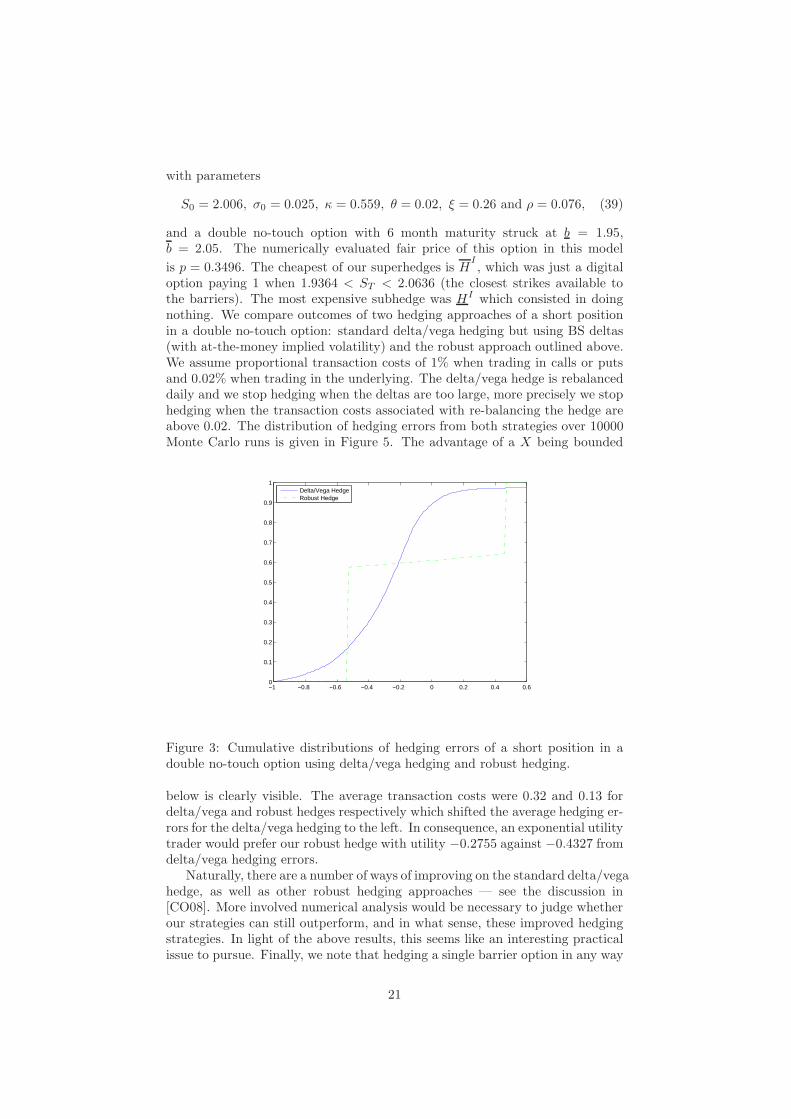
option paying 1 when 1.9364 < ST < 2.0636 (the closest strikes available tothe barriers). The most expensive subhedge was HI which consisted in doingnothing. We compare outcomes of two hedging approaches of a short positionin a double no-touch option: standard delta/vega hedging but using BS deltas(with at-the-money implied volatility) and the robust approach outlined above.We assume proportional transaction costs of 1% when trading in calls or putsand 0.02% when trading in the underlying. The delta/vega hedge is rebalanceddaily and we stop hedging when the deltas are too large, more precisely we stophedging when the transaction costs associated with re-balancing the hedge areabove 0.02. The distribution of hedging errors from both strategies over 10000Monte Carlo runs is given in Figure 5. The advantage of a X being bounded

−1 −0.8 −0.6 −0.4 −0.2 0 0.2 0.4 0.60

0.1

0.2

0.3

0.4

0.5

0.6

0.7

0.8

0.9

1

Delta/Vega HedgeRobust Hedge

Figure 3: Cumulative distributions of hedging errors of a short position in adouble no-touch option using delta/vega hedging and robust hedging.

below is clearly visible. The average transaction costs were 0.32 and 0.13 fordelta/vega and robust hedges respectively which shifted the average hedging er-rors for the delta/vega hedging to the left. In consequence, an exponential utilitytrader would prefer our robust hedge with utility −0.2755 against −0.4327 fromdelta/vega hedging errors.

Naturally, there are a number of ways of improving on the standard delta/vegahedge, as well as other robust hedging approaches — see the discussion in[CO08]. More involved numerical analysis would be necessary to judge whetherour strategies can still outperform, and in what sense, these improved hedgingstrategies. In light of the above results, this seems like an interesting practicalissue to pursue. Finally, we note that hedging a single barrier option in any way

21

is impractical due to transaction and operational costs and in practise bankshedge huge portfolios of barrier options rather than a single option. An adapta-tion of our techniques would be thus required before they could be implementedin real markets.

A Weak Arbitrage

In this appendix we are interested in the possible extensions of the pricingoperator from an arbitrage-free set of call prices C(Ki), 0 = K0 < K1 < . . . <KN to include a call C(b) and a digital call option D(b) where b ∈ (Ki, Ki+1),and a call C(b) and a digital call D(b), where b ∈ (Kj , Kj+1) for j ≥ i + 2.

To avoid simple arbitrages if we add in a call option with strike at x ∈(Kl, Kl+1), we need C(x) to satisfy:

C(x) ≤ C(Kl) + (x − Kl)C(Kl+1) − C(Kl)

Kl+1 − Kl

(40)

C(x) ≥ C(Kl) + (x − Kl)C(Kl) − C(Kl−1)

Kl − Kl−1(41)

C(x) ≥ C(Kl+1) − (Kl+1 − x)C(Kl+2) − C(Kl+1)

Kl+2 − Kl+1(42)

so we require these bounds to hold with (x, l) = (b, i) and (x, l) = (b, j). Somefurther simple arbitrages imply D(x) and D(x) satisfy

C(x) − C(Kl+1)

Kl+1 − x≤ D(x) ≤ D(x) ≤ C(Kl) − C(x)

x − Kl

. (43)

Depending on x, one of the lower bounds (41) or (42) may be redundant. Specifi-cally, there exists b∗ ∈ (Ki, Ki+1) such that the right-hand sides agree for x = b∗,(41) is larger for x < b∗, and (42) is larger for x > b∗, and there is a similar pointb∗ ∈ (Kj , Kj+1) at which the corresponding versions of (41) and (42) agree.

We now prove a result which connects the traded prices of these options, theexistence of both model-free arbitrages and weak arbitrages, and the existenceof a model which agrees with a given pricing operator:

Lemma A.1. Recall X given via (1) and (16). Suppose K is finite b, b 6∈ K,(A) holds, and P admits no WA on X . Let XD = X∪(ST −b)+,1ST >b, (ST −b)+,1ST≥b. Then if C(b), D(b), C(b), D(b) satisfy (40)–(43), there exists anextension of P to XD with

P1ST >b = D(b), P(ST−b)+ = C(b), P1ST ≥b = D(b), P(ST−b)+ = C(b)

such that P admits no model-free arbitrage. Conversely, if any of (40)–(43)fail, then there exists a model-free arbitrage.

Moreover, if there is no model-free arbitrage, there is a weak-arbitrage if andonly if either b ≥ b∗,

C(b) = C(Ki+1)−(Ki+1−b)C(Ki+2) − C(Ki+1)

Ki+2 − Ki+1and

C(b) − C(Ki+1)

Ki+1 − b< D(b) ≤ C(Ki) − C(b)

b − Ki

,

(44)

22

or b ≤ b∗,

C(b) = C(Kj)+(b−Kj)C(Kj) − C(Kj−1)

Kj − Kj−1and

C(b) − C(Kj+1)

Kj+1 − b≤ D(b) <

C(Kj) − C(b)

b − Kj

.

(45)Finally, if there is no weak arbitrage, then there exists a (P ,XD)-market model.Furthermore, we can take the model such that C(·) is piecewise linear and haskinks only at K1 < . . . < Ki < b < K < Ki+1 < . . . < Kj < K < b < Kj+1 <. . . < KN , where K, K are additional strikes which can be chosen arbitrary closeto the barriers b and b respectively.

Proof. The existence of a model-free arbitrage if any of (40)–(43) do not holdis straightforward, and can generally be read off from the inequality — e.g. if(42) fails at b, the arbitrage is to buy the call with strike C(b), sell a call with

strike Ki+1 and buy Ki+1−b

Ki+2−Ki+1units of the call with strike Ki+2, and sell the

same number of calls with strike Ki+1.So suppose (40)–(43) hold and extend P to XD with prices as given in the

statement of the lemma. Assume that neither of (44) or (45) hold. Then itis easy to check that we can find a piecewise linear extension of the functionC(·) which passes through each of the specified call prices and satisfies (7)–(8)and (11). Further, C(·) may be taken as in the statement of the Lemma, withK, K arbitrary close to the barriers b, b respectively. Proposition 2.5 then grantsexistence of a (P ,XD)-market model. In particular there is no weak arbitrageand hence no model-free arbitrage.

It remains to argue that if either of (44) or (45) hold then there is a weak-arbitrage, but no model-free arbitrage.

We first rule out a model-free arbitrage. Since, by Proposition 2.4, P onX ∪(ST − b)+, (ST − b)+ admits no WA we must only show that the additionof the digital options does not introduce an arbitrage. Consider initially the casewhere we add simply a digital option at b. Recalling (6), it is therefore sufficientto show that there does not exist an H ∈ Lin(X ∪(ST − b)+, (ST − b)+), suchthat either

1ST >b + H ≥ 0, and PH < −D(b) (46)

or

−1ST >b + H ≥ 0, and PH < D(b). (47)

However, any possible choice of H must be the combination of a sum of calloptions and forward options. Since only finitely many terms may be included, wenecessarily have H as a continuous function in ST : more precisely, for (St) ∈ P,and any ε, δ > 0, there exist paths (S′

t) ∈ P such that S′T ∈ (ST − δ, ST ) and

|H((St)) − H((S′t))| < ε. Clearly, we may also replace the first conclusion with

S′T ∈ (ST , ST + δ).

So suppose (47) holds, and H((St)) < 1 for some (St) ∈ P with ST = b, thenby the continuity property there exist (S′

t) ∈ P such that S′T > b and H((S′

t)) <1, contradicting (47). Hence, we can conclude that if an arbitrage exists for1ST >b, the same portfolio H is an arbitrage for 1ST≥b if P1ST ≥b = D(b).However, it is possible to construct an admissible curve C(·) such that C(·)

23

matches the given prices at the Ki’s and b, and has

−C′−(b) = −D(b) ∈

(

C(b) − C(Ki+1)

Ki+1 − b,C(Ki) − C(b)

b − Ki

]

,

and hence by arguments of Proposition 2.5, there exists a model under whichthe calls and the digital option 1ST ≥b are fairly priced, and so there cannot bean arbitrage. More generally, if we wish to consider adding both digital options,a similar argument will work, the only aspect we need to be careful about isthat we can find a suitable extension to the call price function, however this isguaranteed by assumption (A).

Finally, we construct a weak arbitrage if either of (44) or (45) hold. Suppose(44) holds. Let P be a model, then

(i) if P(ST ∈ (b, Ki+1)) = 0 we sell short the digital option, buy 1Ki+1−b

units

of the call with strike b, and sell the same number of units of the callwith strike Ki+1. By (44) we receive cash initially, but the final payoff isstrictly negative only for ST ∈ (b, Ki+1),

(ii) else P(ST ∈ (b, Ki+1)) > 0 and we purchase 1Ki+1−b

units of the call with

strike b, sell 1Ki+1−b

+ 1Ki+2−Ki+1

units of the call with strike Ki+1 and buy1

Ki+2−Ki+1units of the call with strike Ki+2. By (44) this costs nothing

initially, has non-negative payoff which is further strictly positive payoffin (b, Ki+1).

A similar argument gives weak arbitrage when (45) holds.

Corollary A.2. Suppose P on XD does not admit a model-free arbitrage. Thenfor all ε > 0, there exists a pricing operator Pε on XD such that |PX−PεX | < εfor all X ∈ XD, and such that a (Pε,XD)-market model exists.

Proof. Given the prices of the call and digital options, we can perturb theseprices by some small δ > 0 to get prices which satisfy the no-weak-arbitrageconditions of Lemma A.1: more precisely, if say (44) holds, by taking C(b) =C(b) + δ, and perhaps (if needed to preserve (43)) also D(b) = D(b) + δ

Ki+1−b,

and if necessary, performing a similar operation at b. The corresponding pricingoperator then satisfies the stated conditions.

Proof of Theorem 4.9. Note that we can’t apply directly Lemma 3.1 to deduce(37) as we do not have prices of digital calls. Instead, we will devise superhedges

of HI, H

II(K) and H

III(K) which only use traded options. Recall that i, j are

such that Ki < b < Ki+1 and Kj < b < Kj+1. Consider the following payoffs,presented in Figure 4,

X1 =(ST − Ki−1)+ − (ST − Ki)

+

Ki − Ki−1,

X2 =1

b − Ki

(

(ST − Ki)+ − Ki+2 − b

Ki+2 − Ki+1(ST − Ki+1)+ +

Ki+1 − b

Ki+2 − Ki+1(ST − Ki+2)+

)

,

(48)

24

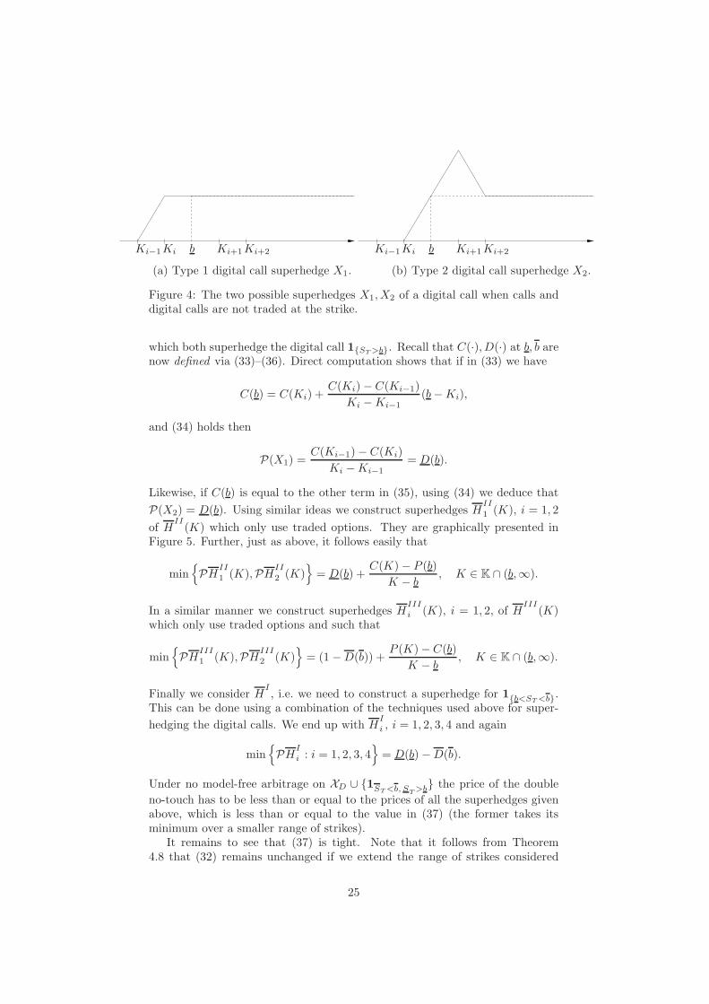
Ki−1Ki Ki+1Ki+2b

(a) Type 1 digital call superhedge X1.

Ki−1Ki Ki+1Ki+2b

(b) Type 2 digital call superhedge X2.

Figure 4: The two possible superhedges X1, X2 of a digital call when calls anddigital calls are not traded at the strike.

which both superhedge the digital call 1ST >b. Recall that C(·), D(·) at b, b arenow defined via (33)–(36). Direct computation shows that if in (33) we have

C(b) = C(Ki) +C(Ki) − C(Ki−1)

Ki − Ki−1(b − Ki),

and (34) holds then

P(X1) =C(Ki−1) − C(Ki)

Ki − Ki−1= D(b).

Likewise, if C(b) is equal to the other term in (35), using (34) we deduce that

P(X2) = D(b). Using similar ideas we construct superhedges HII

1 (K), i = 1, 2

of HII

(K) which only use traded options. They are graphically presented inFigure 5. Further, just as above, it follows easily that

min

PHII

1 (K),PHII

2 (K)

= D(b) +C(K) − P (b)

K − b, K ∈ K ∩ (b,∞).

In a similar manner we construct superhedges HIII

i (K), i = 1, 2, of HIII

(K)which only use traded options and such that

min

PHIII

1 (K),PHIII

2 (K)

= (1 − D(b)) +P (K) − C(b)

K − b, K ∈ K ∩ (b,∞).

Finally we consider HI, i.e. we need to construct a superhedge for 1b<ST <b.

This can be done using a combination of the techniques used above for super-

hedging the digital calls. We end up with HI

i , i = 1, 2, 3, 4 and again

min

PHI

i : i = 1, 2, 3, 4

= D(b) − D(b).

Under no model-free arbitrage on XD ∪ 1ST <b, ST

>b the price of the double

no-touch has to be less than or equal to the prices of all the superhedges givenabove, which is less than or equal to the value in (37) (the former takes itsminimum over a smaller range of strikes).

It remains to see that (37) is tight. Note that it follows from Theorem4.8 that (32) remains unchanged if we extend the range of strikes considered

25

<

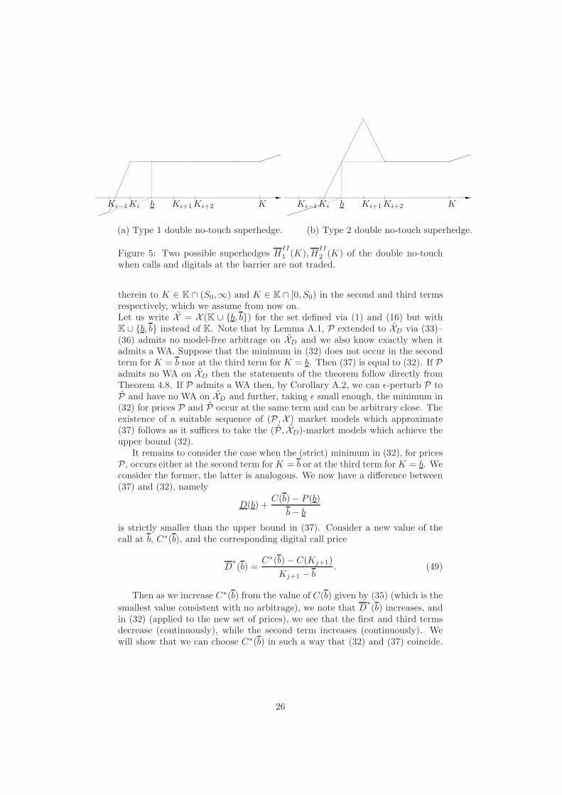
Ki−1Ki Ki+1Ki+2 Kb

(a) Type 1 double no-touch superhedge.

Ki−1Ki Ki+1Ki+2 Kb

(b) Type 2 double no-touch superhedge.

Figure 5: Two possible superhedges HII

1 (K), HII

2 (K) of the double no-touchwhen calls and digitals at the barrier are not traded.

therein to K ∈ K ∩ (S0,∞) and K ∈ K ∩ [0, S0) in the second and third termsrespectively, which we assume from now on.Let us write X = X (K ∪ b, b) for the set defined via (1) and (16) but withK ∪ b, b instead of K. Note that by Lemma A.1, P extended to XD via (33)–(36) admits no model-free arbitrage on XD and we also know exactly when itadmits a WA. Suppose that the minimum in (32) does not occur in the secondterm for K = b nor at the third term for K = b. Then (37) is equal to (32). If Padmits no WA on XD then the statements of the theorem follow directly fromTheorem 4.8. If P admits a WA then, by Corollary A.2, we can ǫ-perturb P toP and have no WA on XD and further, taking ǫ small enough, the minimum in(32) for prices P and P occur at the same term and can be arbitrary close. Theexistence of a suitable sequence of (P ,X ) market models which approximate(37) follows as it suffices to take the (P , XD)-market models which achieve theupper bound (32).

It remains to consider the case when the (strict) minimum in (32), for pricesP , occurs either at the second term for K = b or at the third term for K = b. Weconsider the former, the latter is analogous. We now have a difference between(37) and (32), namely

D(b) +C(b) − P (b)

b − b

is strictly smaller than the upper bound in (37). Consider a new value of thecall at b, C∗(b), and the corresponding digital call price

D∗(b) =

C∗(b) − C(Kj+1)

Kj+1 − b. (49)

Then as we increase C∗(b) from the value of C(b) given by (35) (which is the

smallest value consistent with no arbitrage), we note that D∗(b) increases, and

in (32) (applied to the new set of prices), we see that the first and third termsdecrease (continuously), while the second term increases (continuously). Wewill show that we can choose C∗(b) in such a way that (32) and (37) coincide.

26

Namely, we take

C∗(b) = min

C(Kj+1) − C(Kj+1) − P (b)

Kj+1 − b(Kj+1 − b), C(Kj) + (b − Kj)

C(Kj) − P (b)

Kj − b

(50)and let P∗ denote the pricing operator extended from X to XD via (50), (49)and (33)–(34)). We will show that

(i) P∗ admits no model-free arbitrage on XD,

(ii) the infimum in the second term in (32), for prices P∗, is still attained atb, and this agrees now with the minimum for (37):

infK∈K∩(S0,∞)

C(K) − P (b)

K − b=

C∗(b) − P (b)

b − b; (51)

(iii) the second term in (32) is still the smallest:

C∗(b) − P (b)

b − b≤ −D

∗(b) ≤ −D(b) (52)

D(b) ≤ 1 + infK∈K∩[b,b)∪b

P (K) − C∗(b)

b − K. (53)

If all these conditions hold, and in (i) there is no weak arbitrage, then (32) forP∗ and (37) are equal and applying Theorem 4.8 we get a (P ,X )-market modelwhich achieves the upper bound in (37). If there is a weak arbitrage in (i) wefirst use Corollary A.2 and obtain a sequence of models which approximate (37).The proof is then complete. So we turn to proving the above statements. For(i), we simply need to show that C∗(b) satisfies (40)–(42), i.e.

C(b) ≤ C∗(b) ≤ Kj+1 − b

Kj+1 − Kj

C(Kj) +b − Kj

Kj+1 − Kj

C(Kj+1).

The first inequality follows from the bounds:

C(b) − P (b)

b − b∈

[

C(b) − C(Kj)

b − Kj

,C(Kj+1) − C(b)

Kj+1 − b

]

(54)

which in turn follow from the optimality of b in (32), and the convexity of theprices C(·). The upper bound can be checked by taking a suitable weightedaverage of the terms in (50), where the weights are chosen so that the P (b)term drops out. To show (ii), we note that, by definition of C∗(b), we have

C∗(b) − P (b)

b − b= min

C(Kj) − P (b)

Kj − b,C(Kj+1) − P (b)

Kj+1 − b

and (51) follows from convexity of C and the fact that minimum in the secondterm of (32) for prices P , was attained at b. For (iii), (52) follows from the

definition of D∗(b) and (51), whose value is negative. To deduce (53), we note

the following: suppose (53) fails, so that (rearranging)

1 − D(b) < supK∈K∩[b,b)∪b

C∗(b) − P (K)

b − K. (55)

27

In particular, taking K = b on the RHS we deduce

C∗(b) − P (b)

b − b> 1 − D(b).

which combined with (52) yields 1 − D(b) < −D∗(b) which is clearly a contra-

diction as the first term is non-negative and the second non-positive.

B On the joint law of the maximum and mini-

mum of a UI martingale

Let (Mt : t ≤ ∞) be a uniformly integrable continuous martingale starting at adeterministic value M0 ∈ R and write µ for its terminal law, µ ∼ M∞, where weassume M is non trivial, i.e. µ 6= δM0

. We denote by −∞ ≤ aµ < bµ ≤ ∞ thebounds of the support of µ, i.e. [aµ, bµ] is the smallest interval with µ([aµ, bµ]) =1. In this final appendix, we include some remarks on the joint law of themaximum and minimum of uniformly integrable martingales, namely we studythe function p(b, b) := P

(

M∞ > b and M∞ < b)

for b ≤ M0 ≤ b. Naturally,this is closely related what we have done so far: (Mt) can be interpreted (atleast for aµ ≥ 0) as a market model M u

T−u= Su, u ≤ T , with maturity T call

prices given via (9), and p(b, b) is then the price of a double no-touch option.

Proposition B.1. We have the following properties:

(i) p(M0, b) = p(b, M0) = 0,

(ii) p(b, b) = 1 on [−∞, aµ) × (bµ,∞],

(iii) p is non-increasing in b ∈ (aµ, M0) and non-decreasing in b ∈ (M0, bµ),

(iv) for aµ ≤ b < M0 b and BτJ

< b)

≤ p(b, b) ≤ P(

BτP> b and BτP

< b)

, (56)

where (Bt) is a standard Brownian motion with B0 = M0, τP is the Perkinsstopping time (21) embedding µ and τJ is the Jacka stopping time (23),for barriers (b, b), embedding µ.

The first three assertions of the proposition are clear. Assertion (iv) is areformulation of Lemmas 4.2 and 4.3. It suffices to note that (Bt∧τJ

), (Bt∧τP),

(Mt) are all UI martingales starting at M0 and with the same terminal law µfor t = ∞.

We think of p(·, ·) as a surface defined over the quarter-plane [−∞, M0] ×[M0,∞]. Proposition B.1 describes boundary values of the surface, monotonicityproperties and gives an upper and a lower bound on the surface. However wenote that there is a substantial difference between the bounds linked to the factthat τP does not depend on (b, b) while τJ does. In consequence, the upperbound is attainable: there is a martingale (Mt), namely Mt = (Bt∧τP

), forwhich p is equal to the upper bound for all (b, b). In contrast a martingale(Mt) for which p would be equal to the lower bound does not exist. For themartingale Mt = (Bt∧τJ

), where τJ is defined for some pair (b, b), p will attain

28

the lower bound in some neighbourhood of (b, b) which will be strictly containedin (aµ, M0) × (M0, bµ).

We end this appendix with a result which provides some further insight intothe structure of the bounds discussed above. In particular, we can show somefiner properties of the function p(b, b) and its upper and lower bounds.

Theorem B.2. The function p(b, b) is caglad in b and cadlag in b. Moreover, ifp is discontinuous at (b, b), then µ must have an atom at one of b or b. Further:

(i) if there is a discontinuity at (b, b) of the form:

limwn↓b

p(b, wn) > p(b, b)

then the function g defined by

g(u) = limwn↓b

p(u, wn) − p(u, b), u ≤ b

is non-increasing.

(ii) if there is a discontinuity at (b, b) of the form:

limun↑b

p(un, b) > p(b, b)

then the function h defined by

h(w) = limun↑b

p(un, w) − p(b, w), w ≥ b

is non-decreasing.

And, at any discontinuity, we will be in at least one of the above cases.Finally, we note that the lower bound (corresponding to the tilted-Jacka con-

struction) is continuous in (aµ, M0)× (M0, bµ), and continuous at the boundary(b = bµ and b = aµ) unless there is an atom of µ at either bµ or aµ, while theupper bound (which corresponds to the Perkins construction) has a discontinuitycorresponding to every atom of µ

Before we prove the above result, we note the following useful result, whichis a simple consequence of the martingale property:

Proposition B.3. Suppose that (Mt)t≥0 is a UI martingale with M∞ ∼ µ.Then P(M∞ = b) > 0 implies µ(b) ≥ P(M∞ = b) and

M∞ = b = Mt = b, ∀t ≥ Hb ⊆ M∞ = b a.s..

Proof of Theorem B.2. We begin by noting that by definition of p(b, b), we nec-essarily have the claimed continuity/limiting properties. Further,

lim inf(un,wn)→(u,w)

p(un, wn) ≥ P(M∞ > b and M∞ < b)

andlim sup

(un,wn)→(u,w)

p(un, wn) ≤ P(M∞ ≥ b and M∞ ≤ b).

29

It follows that the function p is continuous at (b, b) if P(M∞ = b) = P(M∞ =b) = 0. By Proposition B.3, this is true when µ(b, b) = 0.

Note that we can now see that at a discontinuity of p, we must be in at leastone of the cases (i) or (ii). This is because discontinuity at (b, b) is equivalentto

P(M∞ ≥ b and M∞ ≤ b) > P(M∞ > b and M∞ < b),

from which we can deduce that at least one of the events

M∞ > b and M∞ = b, M∞ = b and M∞ < b, M∞ = b and M∞ = bis assigned positive mass. However, by Proposition B.3 the final event impliesboth M∞ = b and M∞ = b which is impossible. Consequently, at least one ofthe first two events must be assigned positive mass, and these are precisely thecases (i) and (ii).

Consider now case (i). We can rewrite the statement as: if g(b) > 0, theng(u) is decreasing for u < b. Note however that

g(u) = P(M∞ > u and M∞ ≤ b) − P(M∞ > u and M∞ < b)

= P(M∞ > u and M∞ = b)

which is clearly non-increasing in u. In fact, provided that g(b) < P(M∞ = b),it follows from e.g. [Rog93, Theorem 4.1] that g is strictly decreasing for b >u > supu ≥ −∞ : g(u) = P(M∞ = b). A similar proof holds in case (ii).

We now consider the lower bounds corresponding to the tilted-Jacka con-struction. We wish to show that

P(M∞ ≥ b and M∞ ≤ b) = P(M∞ > b and M∞ < b),

for any (b, b) except those excluded in the statement of the theorem. We notethat it is sufficient to show that P(M∞ = b) = P(M∞ = b) = 0, and byProposition B.3 it is only possible to have an atom in the law of the maximumor the minimum if the process stops at the maximum with positive probability;we note however that the stopping time τJ , due to the definition of Ψµ and Θµ

precludes such behaviour except at the points aµ, bµ.Considering now the Perkins construction, we note from (21) and the fact

that the function γ+µ is decreasing, that we will stop at b only if γ+

µ (M t) = b

and Mt = M t = b. It follows from (18) that there is a range of values (b∗, b∗) for

which γ+µ (b) = b, and consequently, we must have h(b) = P(M∞ = b, M∞ < b)

increasing in b as b goes from b∗ to b∗, with h(b∗) = P(M∞ = b, M∞ < b∗) = 0

and h(b∗) = P(M∞ = b, M∞ < b

∗) = µ(b).8 Similar results for the function

g also follow.

Rogers [Rog93] and Vallois [Val93] described all possible joint laws of (M∞, M∞).This naturally also gives possible joint laws of (M∞, M∞). It would be interest-ing and natural to try to describe possible joint laws of the triple (M∞, M∞, M∞).

Acknowledgement. We are grateful to John Crosby whose comments en-hanced our understanding of FX markets and practicalities of double no-touchoptions and who also provided us with some numerical data from his own work.

8In fact, as above, it follows from e.g. [Rog93, Theorem 2.2] that the maximum must havea strictly positive density with respect to Lebesgue measure, and therefore that the functionh is strictly increasing between the points b∗ and b

∗.

30

References

[AY79] J. Azema and M. Yor. Une solution simple au probleme de Sko-rokhod. In Seminaire de Probabilites, XIII (Univ. Strasbourg, Stras-bourg, 1977/78), volume 721 of Lecture Notes in Math., pages 90–115.Springer, Berlin, 1979.

[BC07] S. Biagini and R. Cont. Model-free representation of pricing rules asconditional expectations. Akahori, Jiro (ed.) et al., Stochastic pro-cesses and applications to mathematical finance. Proceedings of the6th Ritsumeikan International Symposium, Kyoto, Japan, March 6–10, 2006. Hackensack, NJ: World Scientific. 53-84 (2007)., 2007.

[BHR01] H. Brown, D. Hobson, and L. C. G. Rogers. Robust hedging of barrieroptions. Math. Finance, 11(3):285–314, 2001.

[BL78] D. T. Breeden and R. H. Litzenberger. Prices of state-contingentclaims implicit in option prices. Journal of Business, 51(4):621–651,1978.

[Cas08] G. Cassese. Asset pricing with no exogenous probability measure.Math. Finance, 18(1):23–54, 2008.

[CC08] P. Carr and J. Crosby. A class of Levy process models with almostexact calibration to both barrier and vanilla fx options. unpublished,http://www.john-crosby.co.uk/, 2008.

[CH06] A. M. G. Cox and D. G. Hobson. Skorokhod embeddings, minimalityand non-centred target distributions. Probab. Theory Related Fields,135(3):395–414, 2006.

[Che07] A. Cherny. General arbitrage pricing model. III. Possibility approach.In C. Donati-Martin et al., editor, Seminaire de Probabilites XL, vol-ume 1899 of Lecture Notes in Math., pages 463–481. Springer, Berlin,2007.

[CHO08] A. M. G. Cox, D. G. Hobson, and J. Ob loj. Pathwise inequalitiesfor local time: applications to Skorokhod embeddings and optimalstopping. Ann. Appl. Probab., 18(5):1870–1896, 2008.

[CM05] P. Carr and D. P. Madan. A note on sufficient conditions for noarbitrage. Finance Research Letters, 2(3):125–130, 2005.

[CO08] A. M. G. Cox and J. Ob loj. Robust hedging of double touch barrieroptions. unpublished, arXiv:0808.4012v1, 2008.

[Cox04] A. M. G. Cox. Skorokhod embeddings: non-centred target distributions,diffusions and minimality. PhD thesis, University of Bath, 2004.

[Cox08] A. M. G. Cox. Extending Chacon-Walsh: minimality and generalisedstarting distributions. In C. Donati-Martin et al., editor, Seminairede probabilites XLI, volume 1934 of Lecture Notes in Math., pages233–264. Springer, Berlin, 2008.

31

[CW07] P. Carr and L. Wu. Stochastic skew in currency options. Journal ofFinancial Economics, 86(1):213–247, 2007.

[DH06] M. H. A. Davis and D. G. Hobson. The range of traded option prices.To Appear, Math. Finance, 2006.

[DS94] F. Delbaen and W. Schachermayer. A general version of the funda-mental theorem of asset pricing. Math. Ann., 300(3):463–520, 1994.

[Hob98] D. G. Hobson. Robust hedging of the lookback option. Finance Stoch.,2(4):329–347, 1998.

[Jac88] S. D. Jacka. Doob’s inequalities revisited: a maximal H1-embedding.Stochastic Process. Appl., 29(2):281–290, 1988.

[Mij08] A. Mijatovic. Local time and the pricing of time-dependent barrieroptions. To Appear, Finance Stoch., 2008.

[Ob l04] J Ob loj. The Skorokhod embedding problem and its offspring. Probab.Surv., 1:321–390 (electronic), 2004.

[Ob l06] J. Ob loj. A complete characterization of local martingales which arefunctions of Brownian motion and its maximum. Bernoulli, 12(6):955–969, 2006.

[Per86] E. Perkins. The Cereteli-Davis solution to the H1-embedding prob-lem and an optimal embedding in Brownian motion. In Seminar onstochastic processes, 1985 (Gainesville, Fla., 1985), pages 172–223.Birkhauser Boston, Boston, MA, 1986.

[Rog93] L. C. G. Rogers. The joint law of the maximum and terminal valueof a martingale. Probab. Theory Related Fields, 95(4):451–466, 1993.

[Sko65] A. V. Skorokhod. Studies in the theory of random processes. Trans-lated from the Russian by Scripta Technica, Inc. Addison-Wesley Pub-lishing Co., Inc., Reading, Mass., 1965.

[Val93] P. Vallois. On the joint distribution of the supremum and terminalvalue of a uniformly integrable martingale. In Stochastic processesand optimal control (Friedrichroda, 1992), volume 7 of StochasticsMonogr., pages 183–199. Gordon and Breach, Montreux, 1993.

32

Robust pricing and hedging of double no-touch optionsmapamgc/doublenotouch_jan09.pdf · Robust...

Documents

Transcript of Robust pricing and hedging of double no-touch optionsmapamgc/doublenotouch_jan09.pdf · Robust...