Robust Planning for Heterogeneous UAVs in Uncertain ... · Bachelor of Science in Aeronautical and...

Robust Planning for Heterogeneous UAVs in

Uncertain Environments

by

Luca Francesco Bertuccelli

Bachelor of Science in Aeronautical and Astronautical Engineering

Purdue University, 2002

Submitted to the Department of Aeronautics and Astronautics

in partial fulfillment of the requirements for the degree of

Master of Science in Aeronautics and Astronautics

at the

MASSACHUSETTS INSTITUTE OF TECHNOLOGY

June 2004

c© Massachusetts Institute of Technology 2004. All rights reserved.

Author . . . . . . . . . . . . . . . . . . . . . . . . . . . . . . . . . . . . . . . . . . . . . . . . . . . . . . . . . . . . . .

Department of Aeronautics and Astronautics

May 17, 2004

Certified by. . . . . . . . . . . . . . . . . . . . . . . . . . . . . . . . . . . . . . . . . . . . . . . . . . . . . . . . . .

Jonathan P. HowAssociate Professor

Thesis Supervisor

Accepted by . . . . . . . . . . . . . . . . . . . . . . . . . . . . . . . . . . . . . . . . . . . . . . . . . . . . . . . . .Edward M. Greitzer

H.N. Slater Professor of Aeronautics and Astronautics

Chair, Committee on Graduate Students

Robust Planning for Heterogeneous UAVs in Uncertain

Environments

by

Luca Francesco Bertuccelli

Submitted to the Department of Aeronautics and Astronauticson May 17, 2004, in partial fulfillment of the

requirements for the degree ofMaster of Science in Aeronautics and Astronautics

Abstract

Future Unmanned Aerial Vehicle (UAV) missions will require the vehicles to exhibita greater level of autonomy than is currently implemented. While UAVs have mainlybeen used in reconnaissance missions, future UAVs will have more sophisticated ob-jectives, such as Suppression of Enemy Air Defense (SEAD) and coordinated strikemissions. As the complexity of these objectives increases and higher levels of auton-omy are desired, the command and control algorithms will need to incorporate notionsof robustness to successfully accomplish the mission in the presence of uncertaintyin the information of the environment. This uncertainty could result from inherentsensing errors, incorrect prior information, loss of communication with teammates, oradversarial deception.

This thesis investigates the role of uncertainty in task assignment algorithms anddevelops robust techniques that mitigate this effect on the command and controldecisions. More specifically, this thesis emphasizes the development of robust task as-signment techniques that hedge against worst-case realizations of target information.A new version of a robust optimization is presented that is shown to be both com-putationally tractable and yields similar levels of robustness as more sophisticatedalgorithms. This thesis also extends the task assignment formulation to explicitlyinclude reconnaissance tasks that can be used to reduce the uncertainty in the envi-ronment. A Mixed-Integer Linear Program (MILP) is presented that can be solvedfor the optimal strike and reconnaissance mission. This approach explicitly considersthe coupling in the problem by capturing the reduction in uncertainty associated withthe reconnaissance task when performing the robust assignment of the strike mission.The design and development of a new addition to a heterogeneous vehicle testbed isalso presented.

Thesis Supervisor: Jonathan P. HowTitle: Associate Professor

3

Acknowledgments

I would like to thank my advisor, Prof. Jonathan How, who provided much of the

direction and insight for this work. The support of the members of the research group

is also very much appreciated, as that of my family and friends. In particular, my

deep thanks go to Steven Waslander for his insight and support throughout the past

year, especially with the blimp project. The attention of Margaret Yoon in the edit-

ing stages of this work is immensely appreciated.

To my family

This research was funded in part under Air Force Grant # F49620-01-1-0453. The

testbed were funded by DURIP Grant # F49620-02-1-0216.

The views expressed in this thesis are those of the author and do not

reflect the official policy or position of the United States Air Force, De-

partment of Defense, or the U.S. Government.

5

Contents

Abstract 3

Acknowledgements 5

Table of Contents 6

List of Figures 11

List of Tables 14

1 Introduction 17

1.1 UAV Operations . . . . . . . . . . . . . . . . . . . . . . . . . . . . . 17

1.2 Command and Control . . . . . . . . . . . . . . . . . . . . . . . . . 18

1.2.1 Uncertainty . . . . . . . . . . . . . . . . . . . . . . . . . . . . 20

1.3 Overview . . . . . . . . . . . . . . . . . . . . . . . . . . . . . . . . . 21

2 Robust Assignment Formulations 25

2.1 Introduction . . . . . . . . . . . . . . . . . . . . . . . . . . . . . . . 25

2.2 General Optimization Framework . . . . . . . . . . . . . . . . . . . . 25

2.3 Uncertainty Models . . . . . . . . . . . . . . . . . . . . . . . . . . . 27

2.3.1 Ellipsoidal Uncertainty . . . . . . . . . . . . . . . . . . . . . 27

2.3.2 Polytopic Uncertainty . . . . . . . . . . . . . . . . . . . . . . 28

2.4 Optimization Under Uncertainty . . . . . . . . . . . . . . . . . . . . 29

2.4.1 Stochastic Programming . . . . . . . . . . . . . . . . . . . . . 30

2.4.2 Robust Programs . . . . . . . . . . . . . . . . . . . . . . . . 31

7

2.5 Robust Portfolio Problem . . . . . . . . . . . . . . . . . . . . . . . . 33

2.5.1 Relation to Robust Task Assignment . . . . . . . . . . . . . . 33

2.5.2 Mulvey Formulation . . . . . . . . . . . . . . . . . . . . . . . 34

2.5.3 Conditional Value at Risk (CVaR) Formulation . . . . . . . . 35

2.5.4 Ben-Tal/Nemirovski Formulation . . . . . . . . . . . . . . . . 36

2.5.5 Bertsimas/Sim Formulation . . . . . . . . . . . . . . . . . . . 37

2.5.6 Modified Soyster formulation . . . . . . . . . . . . . . . . . . 38

2.6 Equivalence of CVaR and Mulvey Approaches . . . . . . . . . . . . . 39

2.6.1 CVaR Formulation . . . . . . . . . . . . . . . . . . . . . . . . 40

2.6.2 Mulvey Formulation . . . . . . . . . . . . . . . . . . . . . . . 41

2.6.3 Comparison of the Formulations . . . . . . . . . . . . . . . . 41

2.7 Relation between CVaR and Modified Soyster . . . . . . . . . . . . . 42

2.8 Relation between Ben-Tal/Nemirovski and

Modified Soyster . . . . . . . . . . . . . . . . . . . . . . . . . . . . . 43

2.9 Numerical Simulations . . . . . . . . . . . . . . . . . . . . . . . . . . 44

2.10 Conclusion . . . . . . . . . . . . . . . . . . . . . . . . . . . . . . . . 46

3 Robust Weapon Task Assignment 49

3.1 Introduction . . . . . . . . . . . . . . . . . . . . . . . . . . . . . . . 49

3.2 Robust Formulation . . . . . . . . . . . . . . . . . . . . . . . . . . . 50

3.3 Simulation results . . . . . . . . . . . . . . . . . . . . . . . . . . . . 53

3.4 Modification for Cooperative reconnaissance/Strike . . . . . . . . . . 56

3.4.1 Estimator model . . . . . . . . . . . . . . . . . . . . . . . . . 57

3.4.2 Preliminary reconnaissance/Strike formulation . . . . . . . . 58

3.4.3 Improved Reconnaissance/Strike formulation . . . . . . . . . 64

3.5 Conclusion . . . . . . . . . . . . . . . . . . . . . . . . . . . . . . . . 67

4 Robust Receding Horizon Task Assignment 69

4.1 Introduction . . . . . . . . . . . . . . . . . . . . . . . . . . . . . . . 69

4.2 Motivation . . . . . . . . . . . . . . . . . . . . . . . . . . . . . . . . 70

4.3 RHTA Background . . . . . . . . . . . . . . . . . . . . . . . . . . . . 70

8

4.4 Receding Horizon Task Assignment (RHTA) . . . . . . . . . . . . . . 71

4.5 Robust RHTA (RRHTA) . . . . . . . . . . . . . . . . . . . . . . . . 75

4.6 Numerical Results . . . . . . . . . . . . . . . . . . . . . . . . . . . . 75

4.6.1 Plan Aggressiveness . . . . . . . . . . . . . . . . . . . . . . . 87

4.6.2 Heterogeneous Team Performance . . . . . . . . . . . . . . . 89

4.7 RRHTA with Recon (RRHTAR) . . . . . . . . . . . . . . . . . . . . 93

4.7.1 Strike Vehicle Objective . . . . . . . . . . . . . . . . . . . . . 94

4.7.2 Recon Vehicle Objective . . . . . . . . . . . . . . . . . . . . . 94

4.8 Decoupled Formulation . . . . . . . . . . . . . . . . . . . . . . . . . 95

4.9 Coupled Formulation and RRHTAR . . . . . . . . . . . . . . . . . . 96

4.9.1 Nonlinearity . . . . . . . . . . . . . . . . . . . . . . . . . . . 99

4.9.2 Timing constraints . . . . . . . . . . . . . . . . . . . . . . . . 100

4.10 Numerical Results for Coupled Objective . . . . . . . . . . . . . . . 102

4.11 Chapter Summary . . . . . . . . . . . . . . . . . . . . . . . . . . . . 105

5 Testbed Implementation and Development 107

5.1 Introduction . . . . . . . . . . . . . . . . . . . . . . . . . . . . . . . 107

5.2 Hardware Testbed . . . . . . . . . . . . . . . . . . . . . . . . . . . . 108

5.2.1 Rovers . . . . . . . . . . . . . . . . . . . . . . . . . . . . . . 109

5.2.2 Indoor Positioning System (IPS) . . . . . . . . . . . . . . . . 110

5.3 Blimp Development . . . . . . . . . . . . . . . . . . . . . . . . . . . 111

5.3.1 Weight Considerations . . . . . . . . . . . . . . . . . . . . . . 114

5.3.2 Thrust Calibration . . . . . . . . . . . . . . . . . . . . . . . . 114

5.3.3 Blimp Dynamics: Translational Motion (X,Y ) . . . . . . . . 116

5.3.4 Blimp Dynamics: Translational Motion (Z) . . . . . . . . . . 117

5.3.5 Blimp Dynamics: Rotational Motion . . . . . . . . . . . . . . 118

5.3.6 Parameter Identification . . . . . . . . . . . . . . . . . . . . . 118

5.4 Blimp Control . . . . . . . . . . . . . . . . . . . . . . . . . . . . . . 121

5.4.1 Velocity Control Loop . . . . . . . . . . . . . . . . . . . . . . 122

5.4.2 Altitude Control Loop . . . . . . . . . . . . . . . . . . . . . . 122

9

5.4.3 Heading Control Loop . . . . . . . . . . . . . . . . . . . . . . 124

5.5 Experimental Results . . . . . . . . . . . . . . . . . . . . . . . . . . 125

5.5.1 Closed Loop Velocity Control . . . . . . . . . . . . . . . . . . 126

5.5.2 Closed Loop Altitude Control . . . . . . . . . . . . . . . . . . 126

5.5.3 Closed Loop Heading Control . . . . . . . . . . . . . . . . . . 126

5.5.4 Circular Flight . . . . . . . . . . . . . . . . . . . . . . . . . . 128

5.6 Blimp-Rover Experiments . . . . . . . . . . . . . . . . . . . . . . . . 131

5.7 Conclusion . . . . . . . . . . . . . . . . . . . . . . . . . . . . . . . . 133

6 Conclusions and Future Work 135

6.1 Conclusions . . . . . . . . . . . . . . . . . . . . . . . . . . . . . . . . 135

6.2 Future Work . . . . . . . . . . . . . . . . . . . . . . . . . . . . . . . 136

Bibliography 139

10

List of Figures

1.1 Typical UAVs in operation and testing today (left to right): Global

Hawk, Predator, and X-45 . . . . . . . . . . . . . . . . . . . . . . . 18

1.2 Command and Control hierarchy . . . . . . . . . . . . . . . . . . . 19

2.1 Plot relating ω and β . . . . . . . . . . . . . . . . . . . . . . . . . . 42

2.2 Plot relating ω and β (zoomed in) . . . . . . . . . . . . . . . . . . . 42

3.1 Probability Density Functions . . . . . . . . . . . . . . . . . . . . . 54

3.2 Probability Distribution Functions . . . . . . . . . . . . . . . . . . . 55

3.3 Decoupled mission . . . . . . . . . . . . . . . . . . . . . . . . . . . 62

3.4 Coupled mission . . . . . . . . . . . . . . . . . . . . . . . . . . . . . 62

3.5 Comparison of Algorithm 1 (top) and Algorithm 2 (bottom) formula-

tions . . . . . . . . . . . . . . . . . . . . . . . . . . . . . . . . . . . 66

4.1 The assignment switches only twice between the nominal and robust

for this range of µ . . . . . . . . . . . . . . . . . . . . . . . . . . . . 77

4.2 Nominal Mission Veh A (µ = 0) . . . . . . . . . . . . . . . . . . . . 79

4.3 Nominal Mission Veh B (µ = 0) . . . . . . . . . . . . . . . . . . . . 79

4.4 Robust Mission Veh A (µ = 1) . . . . . . . . . . . . . . . . . . . . . 79

4.5 Robust Mission Veh B (µ = 1) . . . . . . . . . . . . . . . . . . . . . 79

4.6 Target parameters for Large-Scale Example. Note that 10 of the 15

targets may not even exist . . . . . . . . . . . . . . . . . . . . . . . 81

4.7 Nominal missions for 4 vehicles, Case 1 (A and B) . . . . . . . . . . 83

4.8 Nominal missions for 4 vehicles, Case 1 (C and D) . . . . . . . . . . 84

11

4.9 Robust missions for 4 vehicles, Case 1 (A and B) . . . . . . . . . . . 85

4.10 Robust missions for 4 vehicles, Case 1 (C and D) . . . . . . . . . . 86

4.11 Expected Scores for Veh A . . . . . . . . . . . . . . . . . . . . . . . 91

4.12 Expected Scores for Veh B . . . . . . . . . . . . . . . . . . . . . . . 91

4.13 Expected Scores for Veh C . . . . . . . . . . . . . . . . . . . . . . . 91

4.14 Expected Scores for Veh D . . . . . . . . . . . . . . . . . . . . . . . 91

4.15 Worst-case Scores for Veh A . . . . . . . . . . . . . . . . . . . . . . 92

4.16 Worst-case Scores for Veh B . . . . . . . . . . . . . . . . . . . . . . 92

4.17 Worst-case Scores for Veh C . . . . . . . . . . . . . . . . . . . . . . 92

4.18 Worst-case Scores for Veh D . . . . . . . . . . . . . . . . . . . . . . 92

4.19 Decoupled, strike vehicle . . . . . . . . . . . . . . . . . . . . . . . . 103

4.20 Decoupled, recon vehicle . . . . . . . . . . . . . . . . . . . . . . . . 103

4.21 Coupled, strike vehicle . . . . . . . . . . . . . . . . . . . . . . . . . 103

4.22 Coupled, recon vehicle . . . . . . . . . . . . . . . . . . . . . . . . . 103

5.1 Overall setup of the heterogeneous testbed: a) Rovers; b) Indoor Po-

sitioning System; c) Blimp (with sensor footprint). . . . . . . . . . 108

5.2 Close-up view of the rovers . . . . . . . . . . . . . . . . . . . . . . . 109

5.3 Close-up view of the transmitter. . . . . . . . . . . . . . . . . . . . 111

5.4 Sensor setup in protective casing showing: (a) Receiver and (b) PCE

board . . . . . . . . . . . . . . . . . . . . . . . . . . . . . . . . . . . 111

5.5 Close up view of the blimp. One of the IPS transmitters is in the

background. . . . . . . . . . . . . . . . . . . . . . . . . . . . . . . . 112

5.6 Close up view of the gondola. . . . . . . . . . . . . . . . . . . . . . 113

5.7 Typical calibration for the motors. Note the deadband region between

0 and 10 PWM units, and the saturation at PWM > 70. . . . . . . 116

5.8 Process used to identify the blimp inertia. . . . . . . . . . . . . . . 119

5.9 Root locus for closed loop velocity control . . . . . . . . . . . . . . 123

5.10 Root locus for closed loop altitude control. . . . . . . . . . . . . . . 124

5.11 Root locus for closed loop heading control. . . . . . . . . . . . . . . 125

12

5.12 Closed loop velocity control . . . . . . . . . . . . . . . . . . . . . . 127

5.13 Closed loop altitude control . . . . . . . . . . . . . . . . . . . . . . 128

5.14 Blimp response to a 90◦ degree step change in heading . . . . . . . 129

5.15 Closed loop heading control . . . . . . . . . . . . . . . . . . . . . . 130

5.16 Closed loop heading error. . . . . . . . . . . . . . . . . . . . . . . . 130

5.17 Blimp flying an autonomous circle . . . . . . . . . . . . . . . . . . . 131

5.18 Blimp-rover experiment . . . . . . . . . . . . . . . . . . . . . . . . . 132

13

List of Tables

2.1 Comparison of [11] and [41] for different values of Γ . . . . . . . . . . 45

2.2 Comparison of [11] and [41] for different levels of robustness. . . . . 45

3.1 Comparison of stochastic and modified Soyster . . . . . . . . . . . . 53

3.2 Comparison of CVar with Modified Soyster . . . . . . . . . . . . . . 56

3.3 Target parameters . . . . . . . . . . . . . . . . . . . . . . . . . . . . 61

3.4 Numerical comparisons of Decoupled and Coupled reconnaissance/Strike

64

4.1 Simulation parameters: Case 1 . . . . . . . . . . . . . . . . . . . . . 76

4.2 Assignments: Case 1 . . . . . . . . . . . . . . . . . . . . . . . . . . . 78

4.3 Performance: Case 1 . . . . . . . . . . . . . . . . . . . . . . . . . . . 78

4.4 Performance: Case 1 . . . . . . . . . . . . . . . . . . . . . . . . . . . 80

4.5 Performance for larger example, λ = 0.99 . . . . . . . . . . . . . . . 89



4.8 Comparison between RWTA with recon and RRHTA with recon . . 99

4.9 Target Parameters . . . . . . . . . . . . . . . . . . . . . . . . . . . . 102

4.10 Visitation times, coupled and decoupled . . . . . . . . . . . . . . . . 104

4.11 Simulation Numerical Results: Case #1 . . . . . . . . . . . . . . . . 104

5.1 Blimp Mass Budget . . . . . . . . . . . . . . . . . . . . . . . . . . . 115

5.2 Blimp and Controller Characteristics . . . . . . . . . . . . . . . . . . 121

15

Chapter 1

Introduction

1.1 UAV Operations

Current military operations are gradually introducing agents with increased levels of

autonomy in the battlefield. While earlier autonomous vehicle missions mainly em-

phasized the gathering of pre- and post-strike intelligence, Unmanned Aerial Vehicles

(UAVs) have recently been involved in real-time strike operations [16, 35, 43]. The

performance and functionality of these vehicles are expected to increase even fur-

ther in the future with the development of mixed manned-unmanned mission and the

deployment of multiple UAVs to execute coordinated search, reconnaissance, target

tracking, and strike missions. However, several fundamental problems in distributed

decision making and control must be solved to ensure that these autonomous vehi-

cles reliably (and efficiently) accomplish these missions. The main issues are high

complexity, uncertainty, and partial/distributed information.

Future operations with UAVs will provide certain advantages over strictly manned

missions. For example, UAVs can be deployed in environments that would endanger

the life of the aircrews, such as in Suppression of Enemy Air Defense (SEAD) missions

with high concentrations of anti-aircraft defenses or in the destruction of chemical

warfare manufacturing facilities. UAVs can also successfully perform surveillance and

reconnaissance missions for periods beyond 24 hours, reducing the fatigue of aircrews

assigned to these operations. An example of these types of high-endurance UAVs is

17

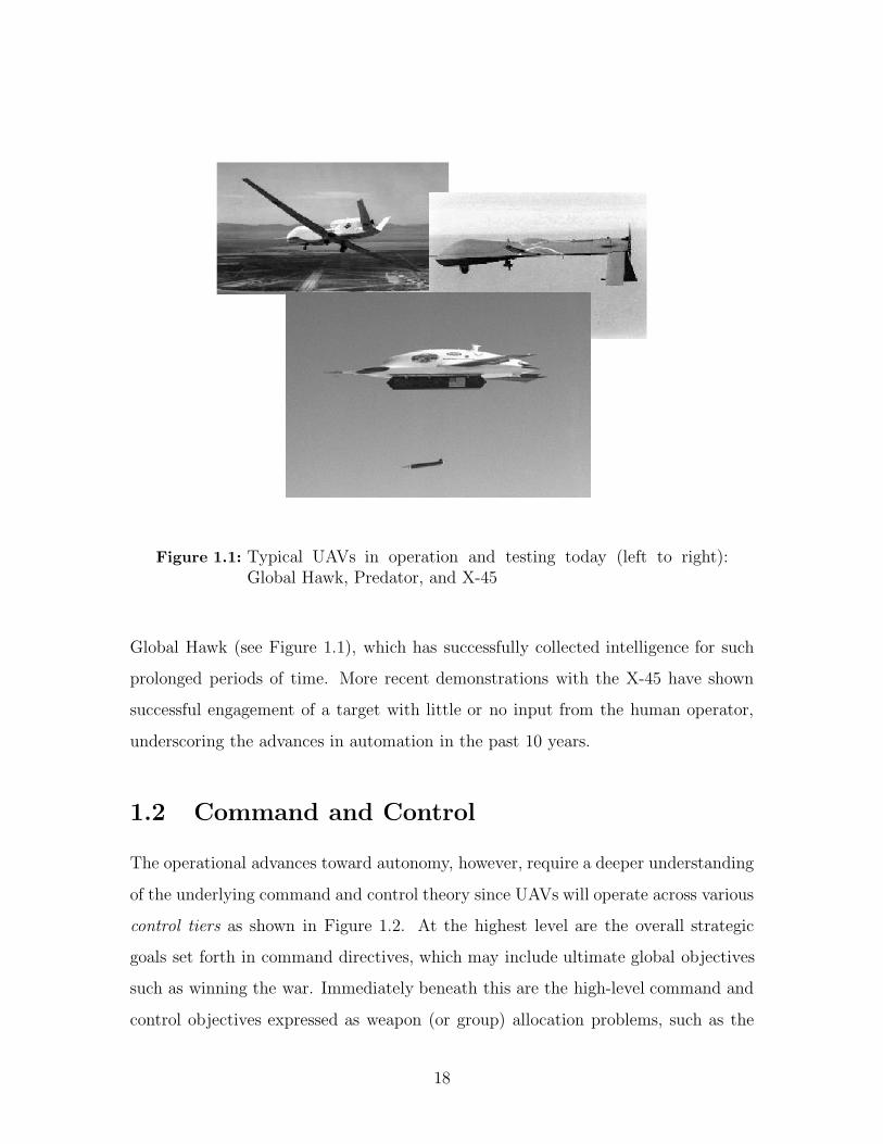
Figure 1.1: Typical UAVs in operation and testing today (left to right):Global Hawk, Predator, and X-45

Global Hawk (see Figure 1.1), which has successfully collected intelligence for such

prolonged periods of time. More recent demonstrations with the X-45 have shown

successful engagement of a target with little or no input from the human operator,

underscoring the advances in automation in the past 10 years.

1.2 Command and Control

The operational advances toward autonomy, however, require a deeper understanding

of the underlying command and control theory since UAVs will operate across various

control tiers as shown in Figure 1.2. At the highest level are the overall strategic

goals set forth in command directives, which may include ultimate global objectives

such as winning the war. Immediately beneath this are the high-level command and

control objectives expressed as weapon (or group) allocation problems, such as the

18

Figure 1.2: Command and Control hierarchy

assignment of a team of UAVs to strike high value targets or evaluate the presence or

absence of threats. At a lower level are the immediate (i.e., more tactical) control

objectives such as generating optimal trajectories that move a vehicle from its current

position to a goal state (e.g., a target). The ∆ij in Figure 1.2 represent disturbances

caused by uncertainty due to sensing errors, lack of (or incorrect) communication, or

even adversarial deception, which are added in the feedback path to the higher-level

control. This captures the typical problem that the information communicated up to

the higher levels of the architecture may be both incorrect or even incomplete –

part of the so-called “fog of war” [45].

To reduce the operator workload and enable efficient remote operations, the UAVs

will have to autonomously execute all levels of the control hierarchy. This will en-

tail information being continuously communicated from the higher-levels to the lower

levels, and vice versa, with the decisions being made based on the current situational

awareness, and the actions chosen affecting the information known about the envi-

ronment. This is inherently a feedback system, since information that is collected by

the sensors is sent to the controllers (in this case, the higher- and lower-level decision

19

makers) which generate a control action (the plans). This command and control hier-

archy requires the development of tools that satisfactorily answer critical questions

of any control system, such as robustness to uncertainty and stability of the overall

closed loop system. This thesis focuses on the robustness of higher-level command

and control systems to the uncertainty in the environment.

1.2.1 Uncertainty

Current autonomous vehicles operate with a multitude of sensors. Apart from the on-

board sensors that measure vehicle health and state, sensors such as video cameras

and Forward-Looking InfraRed (FLIR) provide the vehicles with the capability of

observing and exploring the environment [16, 24, 35, 43]. The human operators at

the base station interpret and make decisions based on the information obtained by

these sensors. Further, databases containing environmental and threat maps are also

primarily updated by the operators (via information sources as AWACS, JSTARS, as

well as ground-based intelligence assets [44]) and sent back to the vehicles, thereby

updating their situational awareness. Future vehicles will make decisions about their

observations and update their situational awareness maps autonomously. The primary

concern is that these sensors and database updates will not be accurate due to inherent

errors, and while a human operator may be able to account for this in the planning and

execution of the commands to the vehicles, algorithms for autonomous higher-level

operation have not yet fully addressed this uncertainty.

The principal source of uncertainty addressed in literature is attributed to sensing

errors [21, 36]. For example, optical sensors introduce noise due to the quantization of

the continuous image into discrete pixels while infrared sensors are impacted by back-

ground thermal noise. There is, however, another significant source of uncertainty

that has to be included as these autonomous missions evolve; namely, the uncertainty

that comes from a priori information, such as target location information from incom-

plete maps [15, 34]. Further, target classification errors and data association errors

may also contribute to the overall uncertainty in the information. Finally, real-time

information from conflicting intelligence sources may introduce significant levels of

20

uncertainty in the decision-making problem.

Mitigating the effect of uncertainty in lower-level planning algorithms has typi-

cally been addressed by the field of robust control. Theory and algorithms have been

developed that make the controllers robust to model uncertainty and sensing or pro-

cess noise. The equivalent approach for robust higher-level decision-making appears

to have received much less attention. The main concern is that the higher-level task

assignment decisions based on nominal information that do not incorporate the un-

certainty in their planning may result in overly optimistic missions. This is an issue

because the performance of these optimistic missions could degrade significantly if

the nominal parameters were replaced by their uncertain estimates.

Work has been done in the area of stochastic programming to attempt to incorpo-

rate the effects of uncertainty in the planning, much of which has been extended to the

area of UAVs [32, 33]. Many of these techniques have emphasized the impact of the

uncertainty on current plans, and not necessarily analyzing the value of information

in future plans. This is in stark contrast to the financial community, which has begun

developing multi-stage stochastic and robust optimization techniques that take into

account the impact of the uncertainty in future stages of the optimization [7, 17]. Cre-

ating planning algorithms that incorporate the future effects of the uncertainty in the

decision-making is a key advancement in the development of robust UAV command

and control decisions.

1.3 Overview

This thesis addresses the impact of uncertainty in higher-level planning algorithms of

task assignment, and develops robust techniques that mitigate this effect on command

and control decisions. More specifically, this thesis emphasizes the development of

robust task assignment techniques that hedge against worst-case target realizations

of target information.

Chapter 2 introduces the general optimization problem analyzed in this thesis

where the problem is modified to include uncertainty and various techniques to make

21

the optimization robust to the uncertainty are introduced. The key contributions in

this chapter are:

• Introduction of a new computationally tractable robust approach (Modified

Soyster) that is shown to be numerically efficient, and yields performance com-

parable to the other robust approaches presented;

• Identification of strong connections between several key previously published

robustness approaches, showing that they are intrinsically related. Numerical

simulations are given to emphasize these similarities.

Chapter 3 introduces the Weapon Target Assignment (WTA) problem [33] as very

general formulation of the problem of allocating weapons to targets. The contribu-

tions of this work are:

• Presentation of the robust WTA (RWTA) that is robust to the uncertainty in

target scores caused by sensing errors and poor intelligence information. Also,

demonstrated the numerical superiority of the RWTA in protecting against the

worst-case while at the same time preserving performance;

• Introduction of a new formulation that incorporates reconnaissance as a mission

objective in the RWTA. This is quantified as a predicted reduction in uncer-

tainty achieved by assigning a reconnaissance vehicle to a target with high

uncertainty.

Chapter 4 presents the Receding Horizon Task Assignment (RHTA) introduced in

Ref. [1], which is a computationally effective method of assigning vehicles in the

presence of side constraints. The key innovations are:

• Development of a robust version of the RHTA (RRHTA) and shown to hedge

the optimization against worst case realizations of the data;

• Modification of the RRHTA to allow for reconnaissance as a vehicle objective.

Numerical results are presented to demonstrate the positive impact of recon-

naissance on the ultimate mission objective.

Chapter 5 introduces a new vehicle (a blimp) to a rover testbed that makes the

testbed truly heterogeneous due to different vehicle dynamics and vehicle objectives.

22

The blimp is used to simulate a reconnaissance vehicle that provides information to

the rovers that simulate strike vehicles. The key contributions of this chapter are:

• Development of a guidance and control system for blimp autonomous flight;

• Demonstration of real-time blimp-rover missions.

The thesis concludes with suggested future work for this UAV task assignment prob-

lem.

23

Chapter 2

Robust Assignment Formulations

2.1 Introduction

This chapter discusses the application of Operations Research (OR) techniques to the

problem of optimally allocating resources subject to a set of constraints. These prob-

lems are initially described in a deterministic framework, with the recognition that

such a framework poses limitations since real-life parameters used in the optimizations

are rarely known with complete certainty. Various robust techniques are presented

as viable methodologies of planning with uncertainty. A robust algorithm resulting

from a modification of the Soyster formulation is introduced (Modified Soyster) as

a new computationally tractable and intuitive robust optimization technique that,

in contrast to existing robust techniques [8, 11, 12], can easily be extended to more

complex problems, such as those introduced in Chapter 4. Strong relationships are

then shown between the various robust optimizations when the uncertainty affects the

objective function coefficients. Finally, the Modified Soyster technique is numerically

evaluated with other robust techniques to demonstrate that the approach is effective.

2.2 General Optimization Framework

The integer optimization problems analyzed in this thesis have a linear objective

function and are subject to linear constraints; the decision variables are restricted to

25

lie in a discrete set, which differs from the continuous set of a linear programming [10].

More specifically, the decision variables in general will be binary, resulting in 0 − 1

integer programming problems, or binary programs (BP). If some of the decision

variables are allowed to lie in a continuous set and the remaining ones are confined

in the discrete set, and the objective function and constraints are linear, then the

problems are known as Mixed-Integer Linear Programs (MILP) [10]. Most of the

problems analyzed in this thesis, however, are BP with linear objective functions and

constraints.

The most general form of the discrete optimization problem is written as

maxx

J = cTx

subject to Ax ≤ b (2.1)

x ∈ XN

where c = [c1, c2, ..., cN]T denotes the objective function coefficients; A and b are the

data in the constraints imposed on the decision variables x = [x1, x2, ..., xN]T . The

vector x is a feasible solution if it satisfies the constraints imposed by A and b. The

constraint x ∈ XN is used to emphasize that the set of decision variables must lie

in a certain set; for the assignment problem in general, this set is the discrete set of

0− 1 integers, X = {0, 1}. More specifically, in the allocation of UAVs for real-world

strike operations, the goal is to destroy as many targets as possible subject to various

constraints. In this case, the decision variable is the allocation of UAVs to targets,

and the objective coefficients could represent target scores. Typical constraints could

be the total number of available vehicles to perform the mission, vehicle attrition due

to adversarial fire, etc. [22, 24, 30, 33, 32].

An example that is closely related to the optimal allocation of weapons to targets

is the integer version of the classic LP portfolio problem [29]. Given n stocks, each

with return ci, the objective is to maximize the total profit subject to investing in

only W stocks. Since only an integer number of items can be picked (we cannot

26

choose half an item), this problem can be written in the above form as

maxx

J =

n∑

i=1

cixi

subject ton∑

i=1

xi ≤ W (2.2)

xi ∈ {0, 1}

In this deterministic framework, this problem can be solved as a sorting problem,

which has a polynomial-time solution.

Many integer programs, however, are extremely difficult to solve, and the solution

time strongly depends on the problem formulation. Many approximations have been

developed to solve these problems more efficiently [10]. Most of these algorithms

have emphasized improving the computational efficiency of the solution, which is a

crucial problem to solve due to the complexity of solving these problems. An equally

important problem to address, however, is the role of uncertainty in the optimization

itself. The parameters used in the optimization are usually the result of either direct

measurements or estimates, and thus cannot generally be considered as perfectly

known. The issue of uncertainty in linear programming is certainly not new [8, 9],

but this issue has only recently been successfully addressed in the integer optimization

community [11, 12]. The next section discusses some models of data uncertainty.

2.3 Uncertainty Models

Various models can be used to capture the uncertainty in a particular problem. The

two types investigated here are the ellipsoidal and polytopic models [37, 39].

2.3.1 Ellipsoidal Uncertainty

An ellipsoidal uncertainty set is frequently used to describe the distribution of many

real-life noise processes. For example, it accurately models the distribution of position

errors in the Indoor Positioning System of Chapter 5. Consider the case of Gaussian

27

random variables c with mean c and covariance matrix Σ. The probability density

function fc(c) of the random variables is given by

fc(c) =1

(2 π)n/2|Σ|1/2exp

{−1

2

[(c − c)TΣ−1(c − c)

]}(2.3)

where |Σ| is the determinant of the matrix Σ. Loci of constant probability density are

found by setting the exponential term in brackets equal to a constant (since the coef-

ficients of the density function are constants). The bracketed term in Equation (2.3)

becomes

(c − c)TΣ−1(c − c) = K (2.4)

which corresponds to ellipsoids of constant probability density (related to K). In the

two-dimensional case, this is the area of the corresponding ellipse.

2.3.2 Polytopic Uncertainty

Polytopic uncertainty is generally used to model data that is known to exist within

certain ranges, but whose distribution within this range is otherwise unknown. This

is the multi-dimensional extension of the standard uniform distribution. This type of

uncertainty model is useful when prior statistical data is unknown, and only intervals

of the data are known. The bounds can be useful for example, in the position estima-

tion of a vehicle that cannot exceed certain physical boundaries. Thus, a constraint

on the position solution is that it has to lie within the boundaries. This could be rep-

resented by a variable c that is constrained to lie in the closed interval [c, c], where

c and c indicate the minimum and maximum values in the interval, respectively.

Mathematically, polytopic uncertainty can be modeled by the set

C(A, b) = { c | A(c − c) ≤ b} (2.5)

where A is a matrix of coefficients that scale the uncertainty and b is the hard con-

straint that bounds the uncertainty. Compared to the ellipsoidal set, this polytopic

uncertainty models guarantees that no realization of the data c will exceed c or be

28

less than c. In the case of ellipsoidal uncertainty, only probabilistic guarantees are

provided that the data realizations will not exceed K.

2.4 Optimization Under Uncertainty

Consider again the portfolio problem from the perspective that the values ci are now

replaced by their uncertain expected returns c. Further assume that these values

belong to an uncertainty set C. The uncertain version of the portfolio problem can

now be written as

maxx

J =n∑

i=1

cixi (2.6)

subject to

n∑

i=1

xi ≤ W (2.7)

xi ∈ {0, 1}, ci ∈ C

If there is no further information on the uncertainty set, this can in general be a

very difficult problem to solve [25]. Incorporating the uncertainty now changes the

meaning of the feasible solution. Without a clear specification on the uncertainty, the

objective function can take various interpretations; i.e., it could become a worst-case

objective or an expected objective. These choices are related to the question of how

to specify the performance for an uncertain optimization; note that this problem

could also contain uncertainties in the constraints (2.7) such as certain probabilistic

bounds on the possibility of bankruptcy. These constraints give rise to the issue of

feasibility, since certain realizations of any uncertain data could cause these prob-

lems to go infeasible. Thus, questions of feasibility in the optimization are also of

critical importance in making the argument for robustness with uncertain mathemat-

ical programs. Both performance and feasibility could be discussed together, but this

thesis investigates performance of the optimization under uncertainty. The role of

uncertainty in the problem of feasibility is addressed in [8, 11] and will be addressed

29

in future research.

2.4.1 Stochastic Programming

A common method for incorporating uncertainty is to use the stochastic programming

approach that simply replaces the uncertain parameters in the optimization, ci, with

the best estimate for those parameters, ci, and solves the new nominal problem [14].

This approach is appealing due to its simplicity, but fundamentally lacks any no-

tion of uncertainty since it does not capture the deviations of the coefficients about

their expected values. This variation is critical in understanding the impact of the

uncertain values on the performance of the optimization. Intuitively, with this sim-

ple approach, two targets having score deviations in the uniformly distributed range

(45, 55) and (30, 70) would be weighted equally since their expected values are both

50. However, choosing the first target is most beneficial in achieving performance

with lower variability.

Another approach in the stochastic programming community is that of scenario-

generation [31].1 This approach generates a set of scenarios that are representative

of the statistical information in the data and solves for the feasible solution that is

a compromise among all the data realizations. This method of incorporating uncer-

tainty critically relies on the number of scenarios used in the optimization, which is a

potential drawback of the approach since increasing the number of scenarios can have

a significant impact on the computational effort to solve the problem. Furthermore,

there is no systematic procedure for determining the minimum number of scenarios

that contain representative statistical characteristics of the entire data set.

1 In some communities, this is a “stochastic program,” while in others it is a “robust optimiza-tion.” Here, it will be introduced as a stochastic program, but in the next section it will be includedin the robust optimization literature to compare it to a very similar approach used in financialoptimization.

30

2.4.2 Robust Programs

Besides stochastic programming approaches of dealing with uncertainty, research in

robust optimization has focused on solving for optimal solutions that are robust to

variations in the data. The general definition used in this thesis for a robust op-

timization is an optimization that maximizes the minimum value of the objective

function. In other words, robust techniques immunize the optimization by protecting

it against the worst-case realizations of the data. The robust version of the single-

stage uncertain portfolio problem is written as

maxx

minc

J =n∑

i=1

cixi (2.8)

subject ton∑

i=1

xi ≤ W (2.9)

xi ∈ {0, 1}, ci ∈ C

where the maximization is done over all possible assignments and the minimization

is over all possible returns. Intuitively, this approach hedges the optimization against

the worst-case realization of the data by selecting returns that have a high worst-case

score. The key point is that the uncertainty is incorporated explicitly in the problem

formulation by maximizing over the minimum value of the optimization, whereas

in the stochastic programming scenario-based approaches there is only an implicit

representation of this uncertainty.

Incorporating uncertainty in the optimization is not new in the financial com-

munity, with its roots in the classic mean-variance portfolio optimization work by

Markowitz [29]. In this classic problem, an investor seeks to maximize the return in

a portfolio at the end of the year,∑

i ciyi, by accounting for the effect of uncertainty

in the elements of the portfolio. This uncertainty is modeled as the variance of the

return, expressed as∑

i σ2i y

2i . The problem is written as

31

Markowitz Problem

maxy

J =n∑

i=1

(ciyi − ασ2

i y2i

)(2.10)

subject to yi ∈ Y

where ci denotes the expected value of the individual elements of the portfolio (for

example, stocks), and σi denotes the standard deviation of the values of each of these

elements. Here, the uncertainty is assumed to decrease the total profit. yi ∈ Y

denotes general constraints, such as an inequality on the total number of investments

that can be made in this time period or a probabilistic constraint on the minimum

return of the investment. In this particular example, the previous assumptions of

integrality for the decision variables are relaxed, and this problem is no longer a

linear program, but reduces to a quadratic optimization problem.2 The variable α

is a tuning parameter that trades off the effect of the uncertainty with the expected

value of the portfolio. Thus, an investor who is completely risk-averse would choose

a large value of α, while an investor who is not concerned with risk would choose a

lower value of α. Choosing α = 0 collapses the problem to a deterministic program

(where the uncertain investment values are replaced by their expectations), but this

is likely to result in an unsafe policy if the portfolio data have large uncertainty.

The framework established by Markowitz is now a common approach used in

finance to hedge against risk and uncertainty [48]. This approach allows an investor

to be cognizant of uncertainty when choosing where to allocate resources, based on

the notion that the resources have an uncertain value. Thus, the Markowitz approach

primarily deals with the performance criteria of optimization.

The next section introduces various formulations for solving the robust portfolio

problem. In the cases when the uncertainty impacts the cost coefficients, strong

similarities are shown between the different robust formulations by presenting bounds

on their objective functions.

2 Note however, that in the case of a zero-one IP, the term y2i ≡ yi, and thus the problem is still

a linear integer program.

32

2.5 Robust Portfolio Problem

This section returns to the portfolio optimization. Analyzing this problem provides

insight to the various robust optimization approaches and will also help establish

relationships among the different techniques.

The notation is slightly changed to be consistent with the UAV assignment.

There are NT elements that can be included in the portfolio, but only an inte-

ger number NV (NV < NT ) can be picked. The expected score of the elements

are c = [c1, c2, . . . , cNT]T ; the standard deviation of the elements is given by σ =

[σ1, σ2, . . . , σNT]T . Each element has a value of ci, where it is assumed that the re-

alizations of the elements are constrained to lie in the interval ci ∈ [ci − σi, ci + σi].

Thus, the problem is to maximize the return of the portfolio, which is given by the

sum of the individual (uncertain) values of the chosen elements

maxx

minc

J =

NT∑

i=1

cixi (2.11)

subject to

NT∑

i=1

xi = NV (2.12)

ci ∈ [ci − σi, ci + σi]

xi ∈ {0, 1}

2.5.1 Relation to Robust Task Assignment

The robust portfolio problem and robust planning algorithms developed in this thesis

are intrinsically related. Both robust formulations want to avoid the worst-case per-

formance in the presence of the uncertainty. For the single-stage portfolio problem in

financial optimization, the investor wants to avoid the worst-case and hedge against

this risk without paying a heavy penalty on the overall performance (namely, the

profit). The objective for the UAV is precisely the same: hedge against the worst-

case realization of target scores, while maintaining an acceptable level of performance

(measured by the overall mission score). Furthermore, the choice of each item to

place in the portfolio is a direct parallel to choosing a specific UAV to accomplish

33

a certain task. For simplicity, for the rest of the section both of the problems are

treated equivalently.

Robust formulations to solve the robust portfolio problem in the LP form already

exist in literature, and their integer counterparts will be presented in this section.

They will be analyzed based on the assumption that uncertainty impacts the objective

function. These formulations are: i) Mulvey; ii) CVaR; iii) Ben-Tal/Nemirovski; iv)

Bertsimas-Sim; and v) Modified Soyster.

2.5.2 Mulvey Formulation

The Mulvey formulation [31] in its most general sense optimizes the expected score,

subject to a term that penalizes the variation about the expected score based on

scenarios of the data. These scenarios contain realizations of the uncertain data (the

values) based on the data statistical information; intuitively, this formulation includes

numerous data realizations and uses them to construct an assignment that is robust

to this variation in the data. The Mulvey approach solves the problem

maxx

J =

NT∑

i=1

(cixi − ωρ(E, x)) (2.13)

NT∑

i=1

xi = NV

xi ∈ {0, 1}

where the function ρ(E, x) is a penalty function based on an error matrix E ≡ c − c

and the assignment vector x, and ω is a weighting on this penalty function. Various

alternatives for the penalty ρ(E, x) can be used, but the two principal ones are

• Quadratic penalty ρ(E, x) =∑

i

∑j Eijxixj – Here E corresponds to a matrix

of errors, and this type of penalty can be used if positive and negative deviations

of the data are both undesirable;

• Negative deviations ρ(E, x) =∑

i max{0,∑

j Eijxj} – This type of a penalty

should be used if negative deviations of the data are undesirable, for example if

34

a certain non-negative objective is always required by the problem statement.

These representation of the penalty functions are not unique. Further, the choice of

penalty will depend on the problem formulation, but note that the quadratic penalty

will change any LP to a quadratic program. The second form can be embedded in

a linear program using slack variables, and thus is the form used in this thesis. The

error matrix is generally found by subtracting the expected scores from each of the

realizations of the scores

E = [E1 | E2 | . . . | EN ]T = [ c1 − c | c2 − c | . . . | cN − c ]T (2.14)

where Ek denotes the kth column of the matrix and ck is the kth realization of the

target scores.

2.5.3 Conditional Value at Risk (CVaR) Formulation

The CVaR approach [26] also uses realizations of the target scores and has a parameter

that penalizes the weight of the variations about the expected score. CVaR solves

the optimization

maxx

J =

NT∑

i=1

cixi −1

N(1 − β)

N∑

m=1

(y − cTmx)+ (2.15)

subject to

NT∑

i=1

xi = NV

xi ∈ {0, 1}

where N denotes the total number of realizations (scenarios) considered, β is a pa-

rameter that probabilistically describes the percentage loss that an operator is willing

to accept from the optimal score, and (g)+ ≡ max(g, 0). For a higher level of pro-

tection, β ≈ 0.99, meaning that the operator desires the probability of loss to be less

than 1%. (Substituting this value for β results in a summation coefficient of 100N

.)

For two scenarios (N = 2), this gives a coefficient of 50, which then heavily penalizes

the importance of non-zero deviation from the optimal assignment (in the summation

35

term). As the number of scenarios is increased, this penalty continually decreases so

that when 300 scenarios are used, the coefficient is decreased to 0.33.

In order to deal exclusively with the non-zero deviations from the mean, define

the set M0,i = {m | (gm)+ 6= 0} and rewrite the optimization as

maxx

J = cT x − 1

N(1 − β)

∑

m∈M0,i

(cT − cTm)x (2.16)

NT∑

i=1

xi = NV

xi ∈ {0, 1}

Rewriting the problem in this form emphasizes that the optimization is penalizing

the expected score obtained by the non-negative variations about the expected score,

which corresponds to the second term.

2.5.4 Ben-Tal/Nemirovski Formulation

The robust formulation of [8] specifies an ellipsoidal uncertainty set for the data that

results in a nonlinear optimization problem that is parameterized by the variable

θ, which allows the designer to vary the level of robustness in the solution. This

parameter has a probabilistic interpretation resulting from the representation of the

uncertainty set. There are many motivating factors for assuming this type of uncer-

tainty set, the principal one being that measurement errors are typically distributed

in an ellipsoid centered at the mean of the distribution.

This model of uncertainty changes the original LP optimization to a Second-

Order Conic Program (SOCP). While attractive from a modeling viewpoint, this

approach does not extend well to an integer formulation. While SOCP are convex,

and numerous interior-point solvers have been developed to solve them efficiently,

SOCP with integer variables are much harder to solve.

36

The target scores c are assumed to lie in an ellipsoidal uncertainty set C given by

C =

{ci |

NT∑

i=1

σ−2i (ci − ci)

2 ≤ θ2

}(2.17)

The robust optimization of Ben-Tal/Nemirovski is

maxx

J = cT x− θ√

V (x) (2.18)

subject to

NT∑

i=1

xi = NV

xi ∈ {0, 1}

where V (x) ≡∑NT

i=1 σ2i x

2i . Again, it is emphasized that when the decision variables

xi are enforced to be integers, the problem becomes a nonlinear integer optimiza-

tion problem, and the difficulty in obtaining the optimization efficiently is increased

significantly.

2.5.5 Bertsimas/Sim Formulation

The formulation proposed in [11] assumes that only a subset of all the target scores

are allowed to achieve their worst cases. The premise here is that, without being too

specific about the probability density function, worst-case variations in the parameters

are expected, but it is unlikely that more than a small subset will be at their worst

value at the same time. The problem to solve is

maxx

J =

NT∑

i=1

cixi + min

{∑

i∈NT

dixiui

}(2.19)

subject to

NT∑

i=1

xi = NV

NT∑

i=1

ui ≤ Γ

xi ∈ {0, 1} , 0 ≤ ui ≤ 1

37

where Γ is the total number of parameters that are allowed to simultaneously be at

their worst-case values, which can be used as a tuning parameter to specify the level

of robustness in the solution. This number need not be an integer, and for example,

if it is specified at 2.5, this implies that two parameters will go to their worst-case,

and one parameter will go to half its worst-case. The variable di is a variation about

the nominal score ci. This optimization can be solved in a polynomial number of

iterations with the algorithm presented in [12].

Bertsimas-Sim Algorithm

Find J∗ = maxxl

J l (2.20)

where ∀l = 1, 2, . . . , NT + 1

J l = Γdl + maxx

(cT x +

∑lp=1(dp − dl)xp

)

subject to

NT∑

i=1

xi = NV

xi ∈ {0, 1}

The key point of this approach is that if the original discrete combinatorial optimiza-

tion problem is solvable in polynomial time, then the robust discrete optimization

of Eq. 2.20 is also solvable in polynomial time, since one is solving a linear number

of nominal optimization. The size of the robust optimization does not scale with

the value Γ; rather it strictly depends on the number of distinct variations di. The

work of Bertsimas and Sim originally focused on the issue of feasibility. Probabilistic

guarantees are provided so that if Γ has been chosen incorrectly, and more than Γ

coefficients actually go to their worst-case, the solution will still be feasible with high

probability [11].

2.5.6 Modified Soyster formulation

The Modified Soyster formulation [13, 41] is a modification of a conservative formula-

tion, which does not allow the operator to tune the level of robustness. The original

Soyster formulation solves an optimization problem by replacing the expected target

scores ci with the 1σ deviation from the expected target scores, ci − σi. Recognizing

38

that this is a potentially conservative approach, the Modified Soyster formulation

solves the problem by introducing a parameter µ that restricts the deviation of the

target scores. It solves the optimization

maxx

J =

NT∑

i=1

(ci − µiσi)xi (2.21)

subject to

NT∑

i=1

xi = NV

xi ∈ {0, 1}

The parameter µi in general is a scalar µ that captures the risk-aversion or accep-

tance of the user by tuning the robustness of the solution. It effectively adds the level

of uncertainty that is introduced in the optimization, where the level is captured by

the standard deviation of the uncertain values ci.

Comments On the Formulations: When robust optimizations are introduced

both based on uncertainty assumptions and computational tractability, the question

of conservatism always arises. This question can be addressed by evaluating the

change in the (optimal) objective value J∗ of the robust solution. With a given

assignment x, bounds between some of the robust optimizations are made relating

these robust optimizations, and analytically investigating the issue of conservatism

among the different techniques. The next section introduces an inequality that is

used in Section 2.7. Next, the relations between the various robust formulations are

demonstrated.

2.6 Equivalence of CVaR and Mulvey Approaches

This section draws a strong connection between the CVaR and Mulvey approaches of

robust optimization.

39

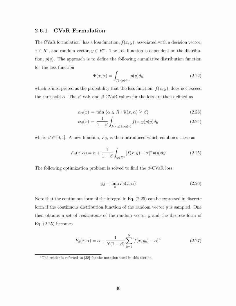
2.6.1 CVaR Formulation

The CVaR formulation3 has a loss function, f(x, y), associated with a decision vector,

x ∈ Rn, and random vector, y ∈ Rm. The loss function is dependent on the distribu-

tion, p(y). The approach is to define the following cumulative distribution function

for the loss function

Ψ(x, α) =

∫

f(x,y)≤α

p(y)dy (2.22)

which is interpreted as the probability that the loss function, f(x, y), does not exceed

the threshold α. The β-VaR and β-CVaR values for the loss are then defined as

αβ(x) = min (α ∈ R : Ψ(x, α) ≥ β) (2.23)

φβ(x) =1

1 − β

∫

f(x,y)≥αβ(x)

f(x, y)p(y)dy (2.24)

where β ∈ [0, 1]. A new function, Fβ, is then introduced which combines these as

Fβ(x, α) = α +1

1 − β

∫

y∈Rm

[f(x, y)− α]+p(y)dy (2.25)

The following optimization problem is solved to find the β-CVaR loss

φβ = minα

Fβ(x, α) (2.26)

Note that the continuous form of the integral in Eq. (2.25) can be expressed in discrete

form if the continuous distribution function of the random vector y is sampled. One

then obtains a set of realizations of the random vector y and the discrete form of

Eq. (2.25) becomes

Fβ(x, α) = α +1

N(1 − β)

N∑

k=1

[f(x, yk) − α]+ (2.27)

3The reader is referred to [38] for the notation used in this section.

40

2.6.2 Mulvey Formulation

The robust formulation in [31] investigates robust (scenario-based) solutions. The

optimization problem takes the form

maxx

J = y − ω

N

N∑

i=1

g(y − xTci) (2.28)

subject to x ∈ X (2.29)

Here ci is the ith realization of the profit vector, c. ω is a tuning parameter for

optimality, and xTci is defined as the ith profit function.

2.6.3 Comparison of the Formulations

This comparison results from the observation that a loss function is the negative of

its profit function. In other words f(x) = −xTci. Furthermore, a threshold of α in

the loss function, can be interpreted as a threshold of α ≡ −α in the profit function.

Thus, f(x, yk) ≤ α is equivalent to xT ci ≥ α. By direct substitution in Eq. (2.27)

Fβ(x, α) = −α +1

N(1 − β)

N∑

i=1

[−xTci + α]+ (2.30)

Since minx{Fβ(x, α)} = maxx{−Fβ(x, α)} the minimization of Eq. (2.30) can be

written as the equivalent maximization problem

maxx

{α − 1

N(1 − β)

N∑

k=1

[α − xTci]+

}(2.31)

By comparing Eq. (2.28), it is clear that since y and a are equivalent representations

of the same function

ω ≡ 1

1 − β(2.32)

So the two approaches are intrinsically related via the parameters ω and β. The former

is a tuning knob for optimality, while the latter has probabilistic interpretations for

constraint violations. The relationship between ω and β is shown in Figure 2.1.

41

10−4

10−3

10−2

10−1

100

100

101

102

103

104

β

µ

Plot of µ vs. β

Figure 2.1: Plot relating ω and β

10−1

100

100

101

102

β

µ

Plot of µ vs. β

Figure 2.2: Plot relating ω and β(zoomed in)

It indicates that ω is greater than 1 at β ≈ 0.1, stating mathematically that the

probability of the loss function not exceeding the threshold α is greater than 0.1.

As this probability is further increased, the loss function will not exceed the thresh-

old α with high probability, a trend that occurs with an increasing value of ω. Note

that Ref. [8] used a value of ω = 100 in their simulations, corresponding to β = 0.89.

As β → 1, ω grows unbounded. Thus, as safer policies are sought (in the sense

that losses beyond a certain threshold do not exceed a certain probability), the value

of ω must increase. Since higher values of ω serve as protection against infeasibility,

there is a price in optimality to obtain probabilistic guarantees on performance. There

is a transition zone (i.e., a zone in which small changes in β result in large changes

in ω) for values of β ≥ 0.25.

2.7 Relation between CVaR and Modified Soyster

The relationship between these robust formulations will be based on approximations

and bounds of the objective functions for a fixed assignment vector, x. Recall that

CVaR is based on realizations of the data, cm. Consider the mth realization of the

data for target i given by cm,i. Using the earlier results obtained in the Appendix

42

of this chapter, this result can be substituted in the objective function for CVaR

obtaining

NT∑

i=1

cixi −1

N(1 − β)

NT∑

i=1

∑

m∈M0,i

(ci − cm,i)xi

≤NT∑

i=1

cixi −1

N(1 − β)

NT∑

i=1

(σi

√|M0,i| − 1

)xi (2.33)

which simplifies to

NT∑

i=1

cixi −1

N(1 − β)

NT∑

i=1

(σi

√|M0,i| − 1

)xi =

NT∑

i=1

(ci −

√|M0,i| − 1

N(1 − β)σi

)xi (2.34)

After defining µi ≡√

|M0,i|−1

N(1−β), this is precisely the Modified Soyster formulation in

Eq. (2.22).

2.8 Relation between Ben-Tal/Nemirovski and

Modified Soyster

For these two formulations, the difference between the objective functions depends

on the tightness of the bound. Recall that for a vector Q, ‖Q‖2 ≤ ‖Q‖1. Then define

Q = Px where P = diag(σ1, σ2, ..., σNT), so it follows that

‖Px‖2 =√

xTP T Px ≤ ‖Px‖1

Substituting this result in Eq. (2.19) gives

cx − θ‖Px‖2 ≥ cx − θ‖Px‖1 (2.35)

43

Note that ‖Px‖1 =∑NT

i=1 |σixi|, but since σi > 0 and xi ∈ {0, 1}, then for this case,

‖Px‖1 =∑NT

i=1 σixi. Substituting this into the righthand side of Eq. (2.35) gives

cx − θ‖Px‖1 =

NT∑

i=1

cixi − θ

NT∑

i=1

σixi =

NT∑

i=1

(ci − θσi)xi (2.36)

If µi = θ, ∀ i, Eq. (2.35) (with ‖Px‖2 replaced with ≡√

V (x) ) can be rewritten as

cx − θ√

V (x) ≥NT∑

i=1

(ci − µiσi)xi (2.37)

The left hand side is the Ben-Tal/Nemirovski formulation of the robust optimization

of Section 2.5.4, while the right hand side is the Modified Soyster of Section 2.5.6.

Based on this expression it is clear in this case that the parameters µ and θ play

very similar roles in the optimization: both will reduce the overall mission score. In

the Ben-Tal/Nemirovski framework, the total mission score is penalized by a term

that captures the variability in the scores, thus indicating that the price of immunizing

the assignment to the uncertainty will immediately result in a lower mission score.

The Modified Soyster will also result in a lower mission score since each element is

individually penalized by µσ.

2.9 Numerical Simulations

This section presents some numerical results comparing two robust formulations with

uncertain costs. The motivations is that a formulation with a predefined budget

of uncertainty (Modified Soyster) could actually be suboptimal with respect to a

formulation that allows the user to choose it (Bertsimas–Sim). A modified portfolio

problem from Ref. [8] is used as the benchmark. The problem statement is: given a set

of NT portfolios with expected scores and a predefined uncertainty model, select the

NV portfolios that will give the highest expected profit. Here, the portfolio choices are

constrained to be binary, and (NT , NV ) = (50, 15). The expected scores and standard

44

Table 2.1: Comparison of [11] and [41] for different values of Γ

Optimization J σJ

Γ = 0 19.05 0.17Γ = 15 17.84 0.08Γ = 50 17.84 0.08Robust 17.84 0.08µ = 1Nominal 19.05 0.17

Table 2.2: Comparison of [11] and [41] for different levels of robustness.

Optimization J σJ

µ = 0 19.05 0.17µ = 0.33 18.86 0.16µ = 1 17.84 0.08

deviations, ci and σi are

ci = 1.15 + i0.05

NT(2.38)

σi = 0.0236√

i, ∀i = 1, 2, . . . , NT (2.39)

1000 numerical simulations were obtained for various values of Γ and compared to

the nominal assignment and the Modified Soyster (µ =1). For this simulation, Γ was

varied in the integer range from [0 : 1 : 50].

For Γ < 15, the robust formulation of Ref. [11] resulted in the nominal assign-

ment, and it resulted in the robust assignment of the Modified Soyster formulation

for Γ ≥ 15. Thus, this particular example did not exhibit great sensitivity to the

uncertainty for the integer case, and the numerical results show this. Furthermore,

the protection factor Γ did not add any additional protection beyond the value of 15.

This observation is important, since it clearly indicates that being robust to uncer-

tainty for integer programs must be tackled carefully, since arbitrarily increasing the

protection level may not necessarily provide a more robust solution.

The numerical simulations were then repeated by varying the parameter µ of the

45

Modified Soyster formulation. The results are shown in Table 3.1. For the case

of µ = 0.33, the Modified Soyster optimization has identified an assignment that

had not been found in the Bertsimas–Sim formulation, which results in a 1% loss

in performance, with a 6% improvement in standard deviation. Both the Modified

Soyster and Bertsimas/Sim formulations identify the identical assignment for the

interval of µ ∈ [0.33, 1], however, which results in a 6% loss of performance compared

to the nominal, but a 50% improvement in the standard deviation. These performance

results are quite typical of standard robust formulations. The performance of the

mission is generally sacrificed in exchange for an increased worst-case value for these

mission scores. This performance criterion will be further investigated in the next

chapter.

In conclusion, tuning the parameter µ will not result in a suboptimal performance

of the robust algorithm as compared to the formulation of Bertsimas/Sim. In fact,

the performances for Γ ≥ 15 and µ ≥ 1 are identical.

2.10 Conclusion

This chapter has introduced the problem of optimization under uncertainty and pre-

sented various robust techniques to protect the mission against worst-case perfor-

mance. This chapter has shown that the various robust optimization algorithms are

not independent, and in fact they are very closely related. The key observation is

that each robust optimization penalizes the total cost using one of two methods:

1. Subtracting an element of uncertainty from each score, and solving the (deter-

ministic) optimization;

2. Subtracting an element of the uncertainty from the total score.

A numerical comparison of two different robust optimization methods showed that

these two techniques result in very similar levels of performance.

46

Appendix to Chapter 2

This appendix introduces an inequality used for proving a bound for the CVaR ap-

proach. Consider a set of uncertain target scores with expected value ci, and their N

realizations: cm,i m = 1, . . . , N and ∀i, which come from prior statistical information

about the data. Next, consider the following summation, over all score realizations

and target scores

P =

NT∑

i=1

N∑

m=1

(ci − cm,i)+xi, xi ∈ {0, 1} (2.40)

As before (g)+ = max(g, 0). Now, define the set M0,i = {m | ci − cm,i > 0}, then

P =

NT∑

i=1

∑

m∈M0,i

(ci − cm,i)xi (2.41)

This summation contains only positive elements, since all non-positive elements have

been excluded from the set. The interior summation over the set M0,i is analogous to a

1-norm: w =∑

m∈M0,i(ci−cm,i) =

∑m∈M0,i

|ci−cm,i|. However, by norm inequalities,

for any vector g the 1-norm overbounds the 2-norm, ‖g‖1 ≥ ‖g‖2, and w can be

overbounded with the 2-norm:

w =∑

m∈M0,i

(ci − cm,i) =∑

m∈M0,i

|ci − cm,i| ≥√ ∑

m∈M0,i

(ci − cm,i)2

≥

√∑m∈M0,i

(ci − cm,i)2

√|M0,i| − 1

√|M0,i| − 1 (2.42)

The first term on the righthand side of Eq. (2.42) is related to the sample standard

deviation. Define

σ2M,i =

∑m∈M0,i

(ci − cm,i)2

|M0,i| − 1

47

Assuming that the entities in M0,i are representative of the full set, then σM,i ≈ σi.

Substitution of this result in Eq. (2.40) the final result is

P =

NT∑

i=1

∑

m∈M0,i

(ci − cm,i)+xi ≥

NT∑

i=1

σi

√|M0,i| − 1 xi (2.43)

48

Chapter 3

Robust Weapon Task Assignment

3.1 Introduction

Future UAV missions will require more autonomous high-level planning capabilities

onboard the vehicles using information acquired through sensing or communicating

with other UAVs in the group. This information will include battlefield parameters

such as target identities/locations, but will be inherently uncertain due to real-world

disturbances such as noisy sensors or even deceptive adversarial strategies. This

chapter presents a new approach to the high-level planning (i.e., task assignment)

that accounts for uncertainty in the situational awareness of the environment.

Except for a few recent results [6, 26, 30], the controls community has largely

treated the UAV task assignment problem as a deterministic optimization problem

with perfectly known parameters. However, the Operations Research and finance

communities have made significant progress in incorporating this uncertainty in the

high-level planning and have generated techniques that make the optimization robust

to the uncertainty [8, 11, 27, 41]. While these results have mainly been made available

for Linear Programs (LPs) [8], robust optimization for Integer Programs (IPs) has

recently been provided with elegant and computationally tractable results [12, 27].

The latter formulation allows the operator to tune the level of robustness included by

selecting how many parameters in the optimization are allowed to achieve their worst

case values. The result is a robust design that reflects the level of risk-aversion (or

49

acceptance) of the operator. This is by no means a unique method to tune the robust-

ness, as the operator could want to restrict the worst case deviation of the parameters

in the optimization, instead of allowing only a few to go to their worst case. This

chapter makes the task assignment robust to the environmental uncertainty, creating

designs that are less sensitive to the errors in the vehicle’s situational awareness.

Environmental uncertainty also creates an inherent coupling between the missions

of the heterogeneous vehicles in the team. Future UAV mission packages will include

both strike and reconnaissance vehicles (possibly mixed), with each type of vehicle

providing unique capabilities to the mission. For example, strike vehicles will have

the critical firepower to eliminate a target, but may have to rely on reconnaissance

vehicle capabilities in order to obtain valuable target information. Including this

coupling will be critical in truly understanding the cooperative nature of missions

with heterogeneous vehicles.

This chapter investigates the impact of uncertain target identity by formulating a

weapon task assignment problem with uncertain data. Sensing errors are assumed to

cause uncertainty in the classification of a target. In the presence of this uncertainty,

the objective robustly assign a set of vehicles to a subset of these targets in order to

maximize a performance criterion. This robustness formulation is extended to solve a

mission with heterogeneous vehicles (namely, reconnaissance and strike) with coupled

actions operating in an uncertain environment.

3.2 Robust Formulation

Consider a weapon-target assignment problem – given a set of NT targets and a set

of NV vehicles, the objective to assign the vehicles to the targets to maximize the

score of the mission. Each target has a score associated with it based on the current

classification, and that the vehicle accrues that score if it is assigned to that target.

If a vehicle is not assigned to a target, it receives a score of 0. The mission score

is the sum of the individual scores accrued by the vehicles; in order for the vehicles

to visit the “best” targets, assume that NV < NT . Due to sensing errors, deceptive

50

adversarial strategies, or even poor intelligence, these scores will be uncertain, and

this lack of perfect information must be included in our planning.

The basic stochastic programming formulation of this problem replaces the deter-

ministic target scores with expected target scores [14], and mathematically, the goal

is to maximize the following objective function at time k

maxx

Jk =

NT∑

i=1

ck,ixk,i (3.1)

subject to:

NT∑

i=1

xk,i = NV , xi ∈ {0, 1}

(We henceforth summarize the constraints as x ∈ X.) The binary variable xk,i is 1 if

a vehicle is assigned to target i and zero if it is not, and ck,i represent the expected

score of the ith target at time k. Assume that any vehicle can be assigned to any

target and (for now) all the vehicles are homogeneous.

Robust formulations have been developed to account for uncertainty in the data by

incorporating uncertainty sets for the data [8]. These uncertainty sets can be modeled

in various ways. One way is to generate a set of realizations (or scenarios) based on

statistical information of the data, and using them explicitly in the optimization;

another way is by using the values of the moments (mean and standard deviation)

directly. Using either method, the robust formulation of the weapon task assignment

is posed as

maxx

minc

Jk =

NT∑

i=1

ck,ixk,i

subject to: x ∈ X (3.2)

ck,i ∈ Ck

The optimization becomes to obtain the “best” worst-case score when each ck,i is

assumed to lie in the uncertainty set Ck. Characterization of this uncertainty set de-

pends on any a priori knowledge of the uncertainty. The choice of this uncertainty set

will generally result in different robust formulations that are either computationally

51

intensive (many are NP -hard [25]) or extremely conservative.

One formulation that falls in the latter case is the Soyster formulation [41]. The

appeal of the Soyster formulation however is its simplicity, as will subsequently be

shown. Here a Modified Soyster formulation is applied to integer programs. It allows

a designer to solve a robust formulation in the same manner as an integer program

while allowing a designer to tune the level of robustness desired in the solution. Here,

the expected target scores, ck,i, are assumed to lie in the interval [ck,i−σk,i, ck,i +σk,i],

where σk,i indicates the standard deviation of target i at time k. In this case the

Soyster formulation solves the following problem

maxx

Jk =

NT∑

i=1

(ck,i − σk,i)xk,i


This formulation assigns vehicles to the targets that exhibit the highest “worst-case”

score. Note that the use of expected scores and standard deviations is not restric-

tive; quite the opposite, they are rather general, providing sufficient statistics for the

unknown true target scores. In general, solving the Soyster formulation results in an

extremely conservative policy, since it is unlikely that each target will indeed achieve

its worst case score; furthermore, it is unlikely that each target will achieve this score

at the same time. A straightforward modification is applied to the cost function al-

lowing the operator to accept or reject the uncertainty, by introducing a parameter

(µ) that can vary the degree of uncertainty introduced in the problem. The modified

robust formulation then takes the form

maxx

Jk =

NT∑

i=1

(ck,i − µσk,i)xk,i


µ restricts the µσ deviation that the mission designer expects and serves as a tuning

parameter to adjust the robustness of the solution. Note that µ = 0 corresponds to

the basic stochastic formulation (which relies on expected scores, and ignores second

52

Table 3.1: Comparison of stochastic and modified SoysterOptimization J σJ max min

Stochastic 14.79 6.07 23.50 6.30Robust 14.37 2.11 17.20 11.43

moment information), while µ = 1 recovers the Soyster formulation. Furthermore, µ

need to be restricted to positive scalars; µ could actually be a vector with elements

µi which penalize each target score differently. This would certainly be useful if the

operator desires to accept more uncertainty in one target than another.

3.3 Simulation results

Numerical results of this robust optimization are demonstrated for the case of an

assignment with uncertain data, and compare them to the stochastic programming

formulation ( where the target scores are replaced with the expected target scores).

10 targets having random score ck,i and standard deviation σi were simulated, and

evaluated the assignments generated from the robust and stochastic formulation, when

the scores were allowed to vary in the interval [ck,i − σi, ck,i + σi]. The expected

mission score, standard deviation, minimum, and maximum scores attained in 1000

numerical simulations were compared, and the results may be seen in Table 3.1. The

simulations confirm the expectation that the robust optimization results in a lower

but more certain mission score; while the robust mission score is 2.8% lower than the

stochastic programming score, there is a 65% reduction in the standard deviation of

this resulting score.

This results in less variability in the resulting mission scores, seen by considering

a 2σ range for the mission scores: for the stochastic formulation this is [2.65, 26.93]

while for the robust one this is [10.15, 18.59]. Although the expected mission score

is indeed lower, there is much more of a guarantee for this score. Furthermore,

note that the robust optimization has a higher minimum score in the simulations of

11.43 compared to 6.30 of the stochastic optimization, indicating that with the given

53

0 5 10 15 20 25 300

0.02

0.04

0.06

0.08

0.1

0.12

0.14

0.16

0.18

0.2PDF of the cost (robust and nominal)

RobustNominal

Figure 3.1: Probability Density Functions

bounds on the cost data, the robust optimization has a better guarantee of “worst-

case” performance. This can also be seen in the probability density functions shown

in Figure 3.1 (and the associated probability distribution functions in Figure 3.2). As

the numerical results indicate, the stochastic formulation results in larger spread in

the mission scores than the robust formulation, which restricts the range of possible

missions scores. Thus, while the maximum achievable mission score is lower in the

robust formulation than that obtained by the stochastic one, the missions scores in

the range of the mean occur with much higher probability.

This robust formulation was also compared to the Conditional Value at Risk

(CVaR) formulation in [26] in another series of experiments with 5 strike vehicles

and 10 targets. CVaR is a modified version of the VaR optimization, which allows

the operator to choose the level of “protection” in a probabilistic sense, based on

given number of scenarios (Nscen) of the data. These scenarios are generated from

54

0 5 10 15 20 25 300

0.1

0.2

0.3

0.4

0.5

0.6

0.7

0.8

0.9

1

RobustNominal

Figure 3.2: Probability Distribution Functions

realizations of the data in the range of [ck,i − σi, ck,i + σi]. This optimization can be

expressed as

maxx

JV aR,k = γ +1

Nscen(1 − β)

Nscen∑

m=1

[γ − cTmx]+

subject to: γ ≤N∑

i=1

ck,ixk,i (3.5)

NT∑

i=1

xk,i = NV

xk,i ∈ {0, 1}

Here x is the assignment vector, x = [x1, x2, . . . , xNV]T , cm is the mth realization of

the target score vector, and [g]+ ≡ max(g, 0). In our simulations a value of β = 0.01

is chosen, allowing for a 1% probability of exceeding our “loss function”. The target

scores were varied in same interval as before, [ck,i−σi, ck,i +σi]. This was compared to

the modified Soyster (Robust entry in the table) formulation using a value of µ = 3.

The numerical results can be seen in Table 3.2.

Note that the CVaR approach depends crucially on the number of scenarios; for

lower number of scenarios, the robust assignment generated by CVaR results in higher

expected mission score, but also higher standard deviation. With 50 scenarios, the

55

Table 3.2: Comparison of CVar with Modified SoysterNumber of Scenarios J σJ max min

10 18.01 2.41 22.80 13.2020 17.33 1.87 20.98 13.6250 17.39 1.99 20.98 13.62100 16.51 1.18 18.90 14.10200 16.58 1.31 19.16 14.04500 16.51 1.18 18.90 14.10

Robust 16.51 1.18 18.90 14.10

CVaR approach results in a higher mission score than the robust formulation, but

also has a higher standard deviation. As the number of scenarios is increased to 100,

the CVaR approach results match with the modified Soyster results; note that at 200

scenarios, a different assignment is generated, and the mission score is increased (as

well as standard deviation). Beyond 500 scenarios, the two approaches generated the

same assignments, and thus resulted in the same performance. In the next section,

the modified Soyster formulation is extended to account for the coupling between the

reconnaissance and strike vehicles.

3.4 Modification for Cooperative reconnaissance/Strike

As stated previously, future UAV missions will involve heterogeneous vehicles with

coupled mission objectives. For example, the mission of reconnaissance vehicles is

to reduce uncertainty in the environment and is coupled with the objective of the

strike vehicles (namely, destroying targets in the presence of this uncertainty). First,

the uncertainty and estimation models used in this work are introduced; the robust

formulation is then used to pose and solve a mission with coupled reconnaissance and

strike objectives.

56

3.4.1 Estimator model

For our estimator model, the target’s state at time k is represented by its target type

(i.e. its score). The output of a classification task is assumed to be a measurement

of the target type, corrupted by some sensor noise νk

zk = Hck + νk (3.6)

where ck represents the true target state (assumed constant); νk represents the (as-

sumed zero-mean, Gaussian distributed) sensor noise, with covariance E[ν2k] = R.

The estimator equations for the updated expected score and covariance that result

from this model are [20]

ck+1 = ck + Lk+1(zk+1 − zk+1|k) (3.7)

P−1k+1 = P−1

k + HR−1HT (3.8)

Here, ck represents the estimate of the target score at time k; Lk+1 represents an

estimator gain on the innovations; the covariance Pk = σ2k; and zk+1|k = Hck. Note

that here, H = 1 since the state of the target is directly observed.

It is clear from Eq. (3.8) that the updated estimate relies on a new observation.

However, this observation will only become available once the reconnaissance vehicle

has actually visited the target. As such, at time k, our best estimate of the future

observation (e.g. at time k + 1) is

zk+1|k = E[Hck+1|k + νk+1

]= Hck (3.9)

This expected observation in the estimator equations can be used to update our

57

predictions of the target classification.

ck+1|k = ck|k + Lk+1(zk+1|k − zk+1|k)

= ck + Lk+1(Hck − Hck) = ck (3.10)

P−1k+1|k = P−1

k + HR−1HT (3.11)

This update is the key component of the coupled reconnaissance/strike problem dis-

cussed in this chapter. By rearranging Eq. (3.11) for the scalar case (H = 1), the

modification to the uncertainty in the target classification as a result of assigning a

future reconnaissance task can be rewritten as

σk+1|k =

√σ2

kR

R + σ2k

(3.12)

or equivalently as the difference

σk+1|k − σk = σk

{√R

R + σ2k

− 1

}(3.13)

Note that in the limiting cases R → ∞ (i.e., a very poor sensor), then σk+1|k = σk,

and the uncertainty does not change. In the case of R = 0 (i.e., a perfect sensor) then

σk+1|k = σk = 0 and the uncertainty in the target classification will be eliminated

by the measurement. In summary, these equations present a means to analyze the

expected reduction in the uncertainty of the target type by a future reconnaissance

prior to visiting the target.

3.4.2 Preliminary reconnaissance/Strike formulation

Reconnaissance and strike vehicles have inherently different mission goals – the ob-

jective of the former is to reduce the uncertainty of the information about the envi-

ronment, the objective of the latter is to recover the maximum score of the mission

by destroying the most valuable targets. Thus, it would be desirable for a recon-

naissance vehicle to be assigned to higher variance targets (equivalently, targets with

58

higher standard deviations), while a strike vehicle would likely be assigned to tar-

gets exhibiting the best “worst-case” score. One could then derive an optimization

criterion for these mission objectives as

maxx,y

Jk=

NT∑

i=1

(ck,i − µσk,i)xk,i + µσk,iyk,i

subject to:

NT∑

i=1

yk,i = NV R ,

NT∑

i=1

xk,i = NV S (3.14)

xk,i, yk,i ∈ {0, 1}

Here, xk,i and yk,i represent the assignments for the strike and reconnaissance vehicles

respectively, and the maximization is taken over these assignments. NV S and NV R

represent the total number of strike and reconnaissance vehicles respectively. Note

that this optimization can be solved separately for x and y, as there is no coupling

in the objective function.

With this decoupled objective function, the resulting optimization is straightfor-

ward. However, this approach does not capture the cooperative behavior that is

required between the two types of vehicles. For example, it would be beneficial for

the reconnaissance vehicle to do more than just update the knowledge of the envi-

ronment by visiting the most uncertain targets. Since the ultimate goal is to achieve

the best possible mission score, the reconnaissance mission should be modified to

account for the strike mission, and vice versa. This can be achieved by coupling the

mission objectives and using the estimator results on the reduction of uncertainty due

to reconnaissance.

An objective function that couples the individual mission objectives captures this

cooperation. As mentioned previously, the target’s score will remain the same if a

reconnaissance vehicle is assigned to it (since an observation has not yet arrived to

update its score), but its uncertainty (given by σ) will decrease from σk to σk+1|k. The

result would exhibit truly cooperative behavior in the sense that the reconnaissance

vehicle will be assigned to observe the target whose reduction in uncertainty will prove

most beneficial for the strike vehicles, thereby creating this coupled behavior between

59

the vehicle missions. The optimization for the coupled mission can be written as

maxx,y

Jk =

NT∑

i=1

(ck,i − µσk,i(1 − yk,i) − µσk+1|k,i yk,i

)xk,i

subject to:

NT∑

i=1

yk,i = NV R ,

NT∑

i=1

xk,i = NV S (3.15)

xk,i, yk,i ∈ {0, 1}

This objective function implies that if a target is assigned to be visited by a recon-

naissance vehicle, then yk,i = 1, and thus the uncertainty in target score i decreases

from σk,i to σk+1|k,i. Similarly, if a reconnaissance vehicle is not assigned to target

i, the uncertainty does not change. Note that by coupling the assignment, if both a

strike and reconnaissance vehicle are assigned to target i, the strike vehicle recovers

an improved score.

The objective function can be simplified by combining similar terms to give

maxx,y

Jk =

NT∑

i=1

(ck,i − µσk,i)xk,i + µ(σk,i − σk+1|k,i)xk,iyk,i

Note that this is a nonlinear objective function that cannot be solved as a Mixed-

Integer Linear Program (MILP), but vk,i ≡ xk,iyk,i can be defined as an additional

optimization variable, and constrain it as follows

vk,i ≤ xk,i

vk,i ≤ yk,i (3.16)

vk,i ≥ xk,i + yk,i − 1

vk,i ∈ {0, 1}

This change of variables enables the problem to be posed and solved as a MILP of

60

Table 3.3: Target parametersTarget c σk σk+1

1 20 4 0.31522 22 7 0.3159

the form

Algorithm #1

maxx,y

Jk =

NT∑

i=1

(ck,i − µσk,i)xk,i + µ(σk,i − σk+1|k,i)vk,i

subject to:

NT∑

i=1

yk,i = NV R ,

NT∑

i=1

xk,i = NV S (3.17)

xk,i, yk,i, vk,i ∈ {0, 1}

vk,i ≤ xk,i

vk,i ≤ yk,i (3.18)

vk,i ≥ xk,i + yk,i − 1

The key point with this formulation is that it captures the coupling in the cooperative

heterogeneous mission by assigning the reconnaissance and strike vehicles together,

taking into account the individual missions.

As a straightforward example, consider a 2 target case with one strike and re-

connaissance vehicle to be assigned (Figure 3.3). This problem is simple enough to

visualize and be used as a demonstration of the effectiveness of this approach. The

reconnaissance (R1) and strike (S1) vehicles are represented by ? and ∆, respectively,

and the ith target, Ti, is represented by 2. The expected score of each target is pro-

portional to the size of the box, and the uncertainty in the target score is proportional

to the radius of the surrounding circle . The target parameters for this experiment

are given in Table 3.3 (µ=1).

Figures 3.3 and 3.4 compare the assignments of the reconnaissance and strike ve-

hicle for the decoupled and coupled cases. In the decoupled case, strike vehicle S1

61

2 4 6 8

2

4

6

8

10

12

T1

T2R1

Recon Package

X [m]

Y [m

]

2 4 6 8

2

4

6

8

10

12

T1

T2

S1

Strike Package

X [m]

Y [m

]

Figure 3.3: Decoupled mission

2 4 6 8

2

4

6

8

10

12

T1

T2R1

Recon Package

X [m]

Y [m

]

2 4 6 8

2

4

6

8

10

12

T1

T2

S1

Strike Package

X [m]

Y [m

]

Figure 3.4: Coupled mission

62

is assigned to T1, while reconnaissance vehicle R1 is assigned to T2. Here the opti-

mization is completely decoupled in that the strike vehicle and reconnaissance vehicle

assignments are found independently. In the coupled case, both strike vehicle S1 and

reconnaissance vehicle R1 are assigned to T2. Without reconnaissance to T1, the ex-

pected worst case score is higher in T1; however, with reconnaissance to that target,

uncertainty is reduced for both targets, and T1 then has a higher expected worst score.

Note that with the two formulations, the strike vehicles are assigned to different tar-

gets. This serves to demonstrate that solving the optimization in Eq. (3.15) does not

result in the same assignment as the coupled formulation. This is key: if we were

able to solve the decoupled formulation for the strike vehicle assignments, the recon-

naissance vehicles would be assigned to those targets and the reconnaissance/strike

mission would thus be obtained. As these results show, that is not the case.

To demonstrate these results numerically, a two-stage mission analysis was con-

ducted. In the first stage, the above two optimizations were solved with the target

parameters; after this first stage, the vehicles progressed toward their intended tar-

gets. At the second stage, it was assumed that the reconnaissance vehicle had actually

reached the target to which it was assigned, and thus, there was no uncertainty in

the target score. The optimization in Eq. (3.6) was then solved for the strike vehi-

cle, with the updated target scores (from the reconnaissance vehicle’s observation)

and standard deviations. Note that this target score could have actually been worse

than predicted, as the observation was made only at time of the reconnaissance UAV

arrival; the target that was not visited by the reconnaissance vehicle maintained its

original expected score and uncertainty. In order to compare the two approaches,

the scores accrued by the strike vehicles at the second stage were tabulated and they

were discounted by their current distance to the (possibly new) target to visit. Both

vehicles incurred this score penalty, but since the targets were en route to their pre-

viously intended targets, a re-assignment to a different target incurred a greater score

penalty, and hence reduction in score.

Of interest in this experiment is the time delay between the assignment of the

reconnaissance vehicle to a target, and its observation of that target. Clearly, if a

63

Table 3.4: Numerical comparisons of Decoupled and Coupled reconnais-sance/Strike

Reconnaissance/Strike J σJ

Coupled 61.19 26.56Decoupled 41.50 23.12

reconnaissance vehicle had a high enough speed such that it could update the “true”

state (i.e., score) of the target almost immediately, then the effects of a coupled

reconnaissance and strike vehicle would likely be identical to those obtained in a

decoupled mission, since the strike vehicles would be immediately reassigned. This

time delay however is present in these typical reconnaissance/strike missions; our time

discount “penalty” for a change in reassignment does reflect that a reassignment as

a result of improved information will result in a lower accrued score for the mission.

The numerical results of 1000 simulations are given in Table 3.4, where J indicates

the average mission score of each approach, and σJ indicates the standard deviation of

this score. Note that the score accrued by the coupled approach has a much improved

performance over the decoupled approach. Furthermore, note that the variation of

this mean performance is almost equivalent for the two approaches (though note that

this is troubling for the decoupled approach due to its lower mean). From this simple

example, the coupling between the two types of vehicles is critical.

3.4.3 Improved Reconnaissance/Strike formulation

While the above example shows that the coupled approach performs better than a

decoupled one, using Eq. (3.19) for more complex missions can result in an incomplete

use of resources if there are more reconnaissance vehicles than strike vehicles, or if

reconnaissance is rewarded as a mission objective in its own right. The cost function

mainly rewards the strike vehicles, by improving their score if a reconnaissance vehicle

is assigned to that target. However, it does not fully capture the reward for the

reconnaissance vehicles that are, for example, not assigned to strike vehicle targets.

64

With the previous algorithm, these unassigned vehicles could be assigned anywhere,

but it would be desirable for them to explore the remaining targets based on a certain

criteria. Such a criterion could be to assign them to the targets with the highest

standard deviation, or to targets that exhibit the “best-case” score (ck,i + σk,i) so as

to incorporate the notion of cost in the optimization. Either of these options can be

included by adding a an extra term to the cost function

Algorithm #2

maxx,y

Jk =

NT∑

i=1

(ck,i − µσk,i)xk,i + µ(σk,i − σk+1,i)vk,i

+Kσk,i(1 − xk,i)yk,i (3.19)

For small K this cost function keeps the strike objective as the principal objective of

the mission, while the weighting on the latter part of the cost function assigns the

remaining reconnaissance vehicles to highly uncertain targets.

Since the coupling between reconnaissance vehicles and strike vehicles is captured

in the first part of the cost function, it is appropriate to assign the remaining recon-

naissance vehicles to targets that have the highest uncertainty. The term (1−xk,i)yk,i

captures the fact that these extra reconnaissance vehicles will be assigned to tar-

gets that have not been assigned (recall when the targets are unassigned, xk,i = 0).

Note that this approach is quite general, since the Kσk,i term can be replaced by

any expression that captures an alternative objective function for the reconnaissance

vehicle.

This change in the objective function in shown in Figure 3.5. In this example,

consider the assignment of 3 reconnaissance and 2 strike vehicles (strike assignments

remained identical in both cases), and K = .01. In the earlier formulation, R3 is

assigned to T5, a target with virtually no uncertainty (note that the target score is

virtually certain since it has such a low uncertainty), since in this instance there was no

reward for decreasing the uncertainty in the environment. The extra reconnaissance

vehicle was not assigned for the benefit of the overall mission as it did not improve

the cost function. Note that there is benefit in the extra reconnaissance vehicle going

65

0 2 4 6 8 10 12 14 160

5

10

15

T1

T2

T3

T4

T5

R1R2

R3

Recon Package

X [m]

Y [m

]

0 2 4 6 8 10 12 14 160

5

10

15

T1

T2

T3

T4

T5

R1R2

R3

Recon Package

X [m]

Y [m

]

Figure 3.5: Comparison of Algorithm 1 (top) and Algorithm 2 (bottom) for-mulations

66

to T3 instead of T5 since it will inherently decrease the uncertainty in the environment.

Thus, the modified formulation captures more intuitive results by reducing the

uncertainty in the environment for the vehicles that will visit the remaining targets.

This is not captured by the original formulation, but is captured by the modified

formulation, which optimally allocates resources based on an overall mission objective.

3.5 Conclusion

This chapter has presented a novel approach to the problem of mission planning

for a team of heterogeneous vehicles with uncertainty in the environment. We have

presented a simple modification of a robustness approach that allows for a direct

tuning of the level of robustness in the solution. This robust formulation was then

extended to account for the coupling between the reconnaissance (tasks that reduce

uncertainty) and strike (tasks that directly increase the score) parts of the combined

mission. Although nonlinear, we show that this coupled problem can be solved as a

single MILP. Future work will investigate the use of time discounting explicitly in the

cost function, thereby incorporating the notion of distance in the assignment, as well

as different vehicle capabilities and performance (speed). We are also investigating

alternative representations of the uncertainty in the information of the environment.

67

Chapter 4

Robust Receding Horizon Task

Assignment

4.1 Introduction

This chapter presents an extension of the Receding Horizon Task Assignment (RHTA).

RHTA is a computationally efficient algorithm for assigning heterogeneous vehicles in

the presence of side constraints [1]; the original approach assumes perfect parameter

information, and thus the resulting optimization is inherently optimistic. A modified

algorithm that includes target score uncertainty is introduced by incorporating the

Modified Soyster robustness formulation of Chapter 2. The benefits of using this ap-

proach are twofold. First and foremost, the robust version of the RHTA (RRHTA) is

successfully protected against worst-case realizations of the data. Second, the robust

formulation of the problem maintains the computational tractability of the original

RHTA.

This chapter also introduces the notion of reconnaissance to a group of hetero-

geneous vehicles, thus creating the Robust RHTA with reconnaissance (RRHTAR).

As in the Weapon Task Assignment (WTA) case, the objective functions of both the

reconnaissance and strike vehicles are now coupled and nonlinear. A cutting plane

method is used to convert the nonlinear optimization to linear form. However, in

contrast to the WTA, the reconnaissance and strike vehicles in this problem are also

69

coupled by timing constraints. The benefits of using reconnaissance are demonstrated

numerically.

4.2 Motivation

The assignment problems discussed so far have largely been of a static nature. The

problem formulation has not considered notions of time or distance in the optimiza-

tion; rather, the focus has largely been on robust weapon allocation based on uncer-

tain target value due to sensing or estimation errors. If an environment is relatively

static or if the effectiveness of the weapons does not depend on their deployment

time, the robust (and for the deterministic case, the optimal) allocation of weapons

in a battlefield can be effectively modeled in this way.

There are, however, other very important problems where the problem of assigning

a vehicle to a target is a function of both its uncertain value and the time it takes

to employ a weapon. An example is the timely deployment of offensive weapons

in a very dynamic and uncertain environment, since the targets could be moved by

the adversary and not be reached in time by the weapon. In this framework, the

target value then becomes a function of both its uncertain value and the weapon

time of flight. The uncertainty in the value of the target will have an effect on the

future assignment decisions since this value is scaled by time, and hence the RHTA

algorithm (introduced in the next sections) needs to be extended and made robust to

this uncertainty.

4.3 RHTA Background

Time discounting factors (λt) that scale the target score, give a functional relationship

between target scores and the time to visit these targets; here 0 < λ ≤ 1 and t

denotes time. The target score cw is multiplied by the time-discount to become a

time-discounted score cwλt.

While the use of time discounts trades off the benefit gained by visiting a target

70

with the effort expended to visit the target, this problem can become extremely com-

putationally difficult as the vehicle and target number increase. This is because the

combinatorial problem of enumerating all the possible permutations of target-vehicle

arrangements becomes computationally very difficult for larger problems. Since the

number of permutations increases exponentially, the assignment problem becomes

computationally infeasible as the problem size increases. RHTA was developed to

alleviate these computational difficulties, and is introduced in the next section.

4.4 Receding Horizon Task Assignment (RHTA)

The RHTA algorithm [1] solves a suboptimal optimization in order to recover com-

putational tractability. Instead of considering all the possible vehicle-target permuta-

tions, RHTA only looks at permutations that contain m or fewer targets (out of the

total target list). From this set, the best permutation is picked for each vehicle, and

the first target of that permutation is taken out of the target list for visitation; the

process is then repeated, until all remaining targets have been assigned. Since the

number of permutations is not the entire set of permutations, however, there is now

no guarantee of optimality in the solution. Nonetheless, the work of [1] demonstrates

that m = 2 in general attains a very high fraction of the optimal solution, while m = 3

generally attains the optimal value. The computational times increase significantly

from m = 2 to 3, and m = 2 is used to solve most practical problems.

Mathematically, the RHTA can be formulated as follows. Consider NT targets

with (deterministic) scores [c1, c2, . . . , cNT]; the positions of the NS vehicles are de-

noted by [q1, q2, . . . , qNS], where qj = [xj, yj]

T denotes the x and y coordinate of the

jth vehicle. The objective function that RHTA maximizes is1

J =∑

i∈p

λticixi (4.1)

1Note, the RHTA of [1] includes a penalty function for a constraint on the munitions. Here,unlimited munitions are assumed, so this penalty function is not included.

71

where ci is the value of the ith waypoint, and p is the set of all permutations that are

evaluated in this iteration. Here, each score of each target is discounted by the time

to reach that target. The set of possible target-vehicle permutations are generated,

and the following knapsack problem is solved

maxx

J =

NS∑

v=1

Nvp∑

p=1

cvpxvp (4.2)

subject to

NS∑

v=1

Nvp∑

p=1

avpixvp = 1 (4.3)

Nvp∑

p=1

xvp = 1, ∀v ∈ 1 . . . NS

xvp ∈ {0, 1}

where Nvp is the total number of permutations for vehicle v. Each grouping of targets

in a given permutation is called a petal: for example, in the case m = 2, only two

targets are in each petal. Constraint (4.3) ensures that each vehicle can only visit

one target: avpi is a binary matrix, and avpi = 1 if target i is in the permutation,

p of vehicle v, and 0 otherwise. The remaining constraint enforces that only one

permutation per vehicle is chosen. cvp is a time discounted score that is calculated

outside of the optimization as

cvp =∑

w∈P

λtwcw, ∀v ∈ 1 . . . NS (4.4)

where P contains the waypoints w in the permutation, λtw is the time discount that

takes into account the distance between a vehicle and a waypoint to which it is

assigned; tw is calculated as the quotient of the distance between target w and vehicle

v, and Vref , the vehicle velocity.

In an uncertain environment, estimation and sensing errors will likely give rise

to uncertain information about the environment, such as target identity or distance

to target; thus, in a realistic optimization, both times to target and target identities

are uncertain, belonging to uncertainty sets T and C. The uncertain version of the

72

RHTA can be written to incorporate this as

maxx

J =

NS∑

v=1

Nvp∑

p=1

cvpxvp (4.5)

subject to

NS∑

v=1

Nvp∑

p=1

avpixvp = 1 (4.6)

Nvp∑

p=1

xvp = 1, ∀v ∈ 1 . . . Nv

cvp =∑

w∈P

λtw cw, ∀v ∈ 1 . . . NS (4.7)

xvp ∈ {0, 1} ci ∈ C tw ∈ T

In this thesis, time (or distance) will be considered known with complete certainty;

hence, the uncertainty set T is dropped and only the uncertainty set C is retained.

The focus is solely on the classification uncertainty due to sensing errors,since the

assumption is that this type of uncertainty has a more significant impact on the

resource allocation problem than the localization issues, which will affect the path-

planning algorithms more directly.

In this particular formulation, cvp represents the uncertain permutation score

which is the summation of weighted and uncertain target scores. Thus, the effect

of each target’s value uncertainty is included in all the permutations. Because the

earlier robust formulations applied exclusively to the target scores (and not to permu-

tations), the current formulation cannot be made robust unless the RHTA is rewritten

to isolate the time discounts in a unique matrix. Then, the uncertainty in the target

scores can be uniquely isolated, and the RHTA can be made robust to this uncertainty.

73

This can be done by modifying the objective function with the following steps

J =

NS∑

v=1

Nvp∑

p=1

cvpxvp

=

NS∑

v=1

Nvp∑

p=1

∑

w∈P

λtw cwxvp (By substituting 4.4)

=

NT∑

w=1

Nvp∑

p=1

cwGwpxvp (By defining Gwp ≡∑

w∈P

λtw )

Here Gwp is a matrix of time discounts. An example of this matrix is given below,

for the case of 1 vehicle, 4 targets, and m = 2 (only two targets per petal).

Gwp =

λt01 0 0 0 . . . λt02 λt01 . . . 0 0

0 λt02 0 0 . . . λt21 λt12 . . . 0 0

0 0 λt03 0 . . . 0 0 . . . λt03 λt04

0 0 0 λt04 . . . 0 0 . . . λt34 λt43

(4.8)

The first column of this matrix represents the time discount incurred by only visiting

target 1 from the current location (represented by 0). The fifth column in this matrix

is the time discount by visiting target 2 first, followed by target 1. The next column

represents visiting target 1 first, followed by target 2.

The optimization with the isolated uncertain score coefficients then becomes

maxx

J =Nw∑

w=1

Nvp∑

p=1

cwGwpxvp (4.9)

subject toNv∑

v=1

Nvp∑

p=1

aivpxvp = 1

Nvp∑

p=1

xvp = 1, ∀v ∈ 1 . . . Nv

Xvp ∈ {0, 1}, c ∈ C

This transformation isolates the effect of the target score uncertainty, in a form that

74

can be solved by applying the Modified Soyster algorithm introduced in Chapter 2.

4.5 Robust RHTA (RRHTA)

From the results of Chapter 2, various related optimization techniques exist to make

the RHTA robust to the uncertainty in the objective coefficients; here, the Modified

Soyster approach is used to develop the RRHTA by hedging it against the worst-case

realization of the uncertain target scores.

With an application of the Modified Soyster approach, the uncertain target scores

ci are replaced by their robust equivalents ci − µσi, and robust objective function of

the RHTA then becomes

maxx

minc

J =

Nw∑

w=1

Nvp∑

p=1

cwGwpxvp ⇒ maxx

J =

Nw∑

w=1

Nvp∑

p=1

(cw − µσw) Gwpxvp (4.10)

Numerical results are shown next for the case of a RRHTA with uncertainty in the

target values. The distinguishing feature of this problem is the use of time discounts.

In the WTA problem, only the target scores contribute in the assignment problem,

while here time is also incorporated in the scaling of the target value and uncertainty.

The choice of assigning vehicles to destroy targets thus depends on both the level of

uncertainty (σi and µ) and their relative distance (which is equivalently captured by

time, since the vehicles are assumed to travel at a constant velocity).

4.6 Numerical Results

This section introduces numerical results obtained with the RRHTA. The first exam-

ple demonstrates the value of hedging against a worst-case realization, by appropri-

ately choosing the value of the parameter µ. The second example is a more complex

scenario which gives additional insight in the effectiveness of this robust approach.

75

Table 4.1: Simulation parameters: Case 1

Target ci σi

1 100 902 50 253 100 45

Robust Hedging

The first case consisted of 2 vehicles and 3 targets. The vehicle initial positions were

(0, 0) and (0, 5) respectively; the target positions were (5, 8), (10, 6), and (6, 15) re-

spectively, while target scores were considered to be uncertain, as shown in Table 4.1.

Targets 1 and 3 had identical expected scores, with different uncertainty associated

with them. Targets 1 and 3 have the highest expected score, but in worst case, target

1 results in a lower score than target 2. Since the nominal assignment does not con-

sider the variation in the target score, it will seek to maximize the expected score by

visiting the target with the largest expected scores first, while the robust assignment

will visit the targets with the largest worst-case scores first. The nominal and robust

optimizations were solved for several values of µ (µ = 0, µ = 1), but the optimization

was only sensitive to the values of µ in the range from [0, 0.6] and [0.6, 1]; only two

distinct assignments were generated for these two intervals. The assignment for the

first interval is referred to as the nominal assignment, while the assignment for the

second interval is referred to as the robust assignment. Figure 4.1 shows the range of

µ which resulted in the nominal and robust assignments, with the visible switch at

µ = 0.6. Since the assignments for µ = 0 and µ = 1 correspond to the nominal and

robust assignment, the following analysis only focuses on these two values of µ.

For the case µ = 0, the mission goal is to strictly drive the optimization based

on expected performance without consideration of the worst-case realizations of the

data. The robust approach instead, drives the optimization to consider the full 1σ

deviations of the data. The visitation order for the different assignments are shown

in Table 4.2. The time discounted scores for each of the targets for these visitation

76

0 0.2 0.4 0.6 0.8 1

Nominal

Robust

µ

Assignment vs. µ

Fig.4.1: The assignment switches only twice between the nominal and robust for thisrange of µ

orders are given in parentheses: the nominal case calculated these scores as ciλtw ,

while the robust case calculated these as (ci − µσi)λtw .

The assignments for the two vehicles for the case µ = 0 are shown in Figures 4.2

and 4.3, while the assignments for the robust case (µ = 1) are shown in Figures 4.4

and 4.5. In the figures, the shaded circles represent the expected score of the target;

the inner (outer) circles represent the target worst-case (best-case) score.

As anticipated, the vehicles in the nominal assignment seek to recover the max-

imum expected score with vehicle A visiting target 2, and vehicle B visiting targets

1 and 3. Here, target 1 is assumed to have a very high expected score, and thus is

visited in the first stage of the RHTA; target 3, which has the same expected score is

visited in the second stage, even though this target has a much lower variation in its

score.

77

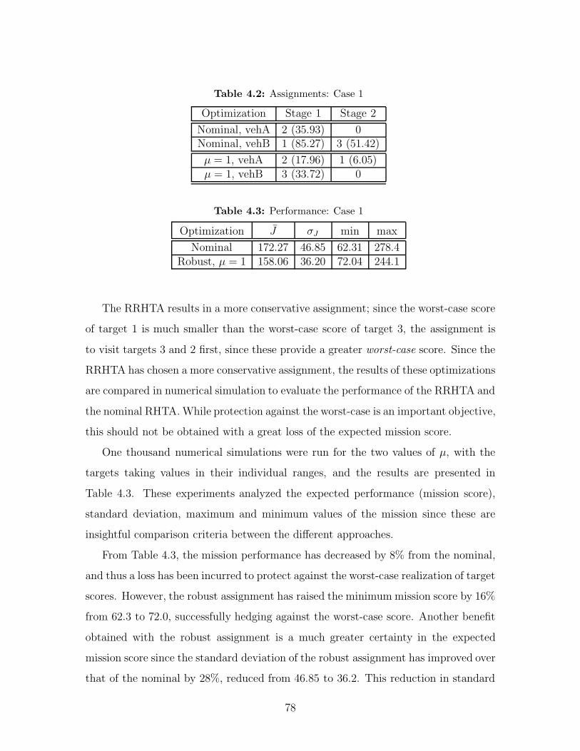
Table 4.2: Assignments: Case 1

Optimization Stage 1 Stage 2

Nominal, vehA 2 (35.93) 0Nominal, vehB 1 (85.27) 3 (51.42)

µ = 1, vehA 2 (17.96) 1 (6.05)µ = 1, vehB 3 (33.72) 0

Table 4.3: Performance: Case 1

Optimization J σJ min max

Nominal 172.27 46.85 62.31 278.4Robust, µ = 1 158.06 36.20 72.04 244.1

The RRHTA results in a more conservative assignment; since the worst-case score

of target 1 is much smaller than the worst-case score of target 3, the assignment is

to visit targets 3 and 2 first, since these provide a greater worst-case score. Since the

RRHTA has chosen a more conservative assignment, the results of these optimizations

are compared in numerical simulation to evaluate the performance of the RRHTA and

the nominal RHTA. While protection against the worst-case is an important objective,

this should not be obtained with a great loss of the expected mission score.

One thousand numerical simulations were run for the two values of µ, with the

targets taking values in their individual ranges, and the results are presented in

Table 4.3. These experiments analyzed the expected performance (mission score),

standard deviation, maximum and minimum values of the mission since these are

insightful comparison criteria between the different approaches.

From Table 4.3, the mission performance has decreased by 8% from the nominal,

and thus a loss has been incurred to protect against the worst-case realization of target

scores. However, the robust assignment has raised the minimum mission score by 16%

from 62.3 to 72.0, successfully hedging against the worst-case score. Another benefit

obtained with the robust assignment is a much greater certainty in the expected

mission score since the standard deviation of the robust assignment has improved over

that of the nominal by 28%, reduced from 46.85 to 36.2. This reduction in standard

78

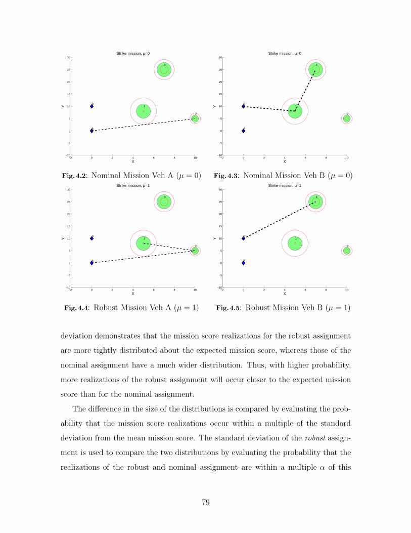
−2 0 2 4 6 8 10−10

−5

0

5

10

15

20

25

30

A

B1

2

3

Strike mission, µ=0

X

Y

Fig.4.2: Nominal Mission Veh A (µ = 0)

−2 0 2 4 6 8 10−10

−5

0

5

10

15

20

25

30

A

B1

2

3


X

Y

Fig.4.3: Nominal Mission Veh B (µ = 0)

−2 0 2 4 6 8 10−10

−5

0

5

10

15

20

25

30

A

B1

2

3


X

Y

Fig.4.4: Robust Mission Veh A (µ = 1)

−2 0 2 4 6 8 10−10

−5

0

5

10

15

20

25

30

A

B1

2

3


X

Y

Fig.4.5: Robust Mission Veh B (µ = 1)

deviation demonstrates that the mission score realizations for the robust assignment

are more tightly distributed about the expected mission score, whereas those of the

nominal assignment have a much wider distribution. Thus, with higher probability,

more realizations of the robust assignment will occur closer to the expected mission

score than for the nominal assignment.

The difference in the size of the distributions is compared by evaluating the prob-

ability that the mission score realizations occur within a multiple of the standard

deviation from the mean mission score. The standard deviation of the robust assign-

ment is used to compare the two distributions by evaluating the probability that the

realizations of the robust and nominal assignment are within a multiple α of this

79

Table 4.4: Performance: Case 1

α Ur Un

1 80.10 83.281.5 94.40 92.512 100.0 98.70

2.5 100.0 99.803 100.0 100.04 100.0 100.0

standard deviation from the means Jr and Jn. The probabilities are given by

Ur ≡ Pr(Jr < |Jr − ασr|) (4.11)

Un ≡ Pr(Jn < |Jn − ασn|) (4.12)

These results are summarized in Table 4.4. The robust assignment results in almost

95% of the realizations data within 1.5 standard deviations of the expected value;

however, the robust assignment has 100% of its realizations within 2 standard devia-

tions, while the nominal has 100% at 3 standard deviations. While both distributions

have all their realizations within the 3 standard deviation range, recall that the robust

realizations of the mission scores had a much tighter distribution than their nominal

counterparts, since the standard deviation of the latter was 28% smaller than the

robust.

Thus, while the robust RHTA has a slightly lower expected mission score than

the nominal, the robust RHTA has protected against the worst-case realization of the

data, and has also reduced the size of distribution of mission score realizations. Next,

a slightly larger example is considered.

Complex Example

In this section, a more complex example consisting of 4 vehicles and 15 waypoints is

considered (λ = .91). For this large-scale simulation, the target scores and uncertain-

ties were randomly generated, and they are shown in Figure 4.6. Here © represents

80

0 2 4 6 8 10 12 14 160

20

40

60

80

100

120

140

160

180

Target Number

Tar

get V

alue

Target parameters for Large−Scale example

Fig. 4.6: Target parameters for Large-Scale Example. Note that 10 of the 15 targetsmay not even exist

the expected target score, and the maximum and minimum deviations are represented

by the error bars. This environment had a very extreme degree of uncertainty in that

10 of the 15 targets had a worst-case score of 0; this represents the fact that in the

worst-case these targets do not exist.2 This extreme case is nonetheless very realistic

in real-world operations due to uncertain intelligence or sensor errors that could be

very uncertain about the existence of a target. Robust optimization techniques must

successfully plan even in these very uncertain conditions. While this large-scale exam-

ple was found to be very sensitive to the various levels of µ, for simplicity the focus will

2Note that higher value targets do not necessarily have a high uncertainty in their scores; hence,this example is distinct from the portfolio problem studied in Chapter 2 where by construction,higher target values have a greater uncertainty.

81

be on µ = 0, 0.5, 0.75, 1. µ = 0 represents the assignment that was generated without

any robustness included, while the other values of µ increase the desired robustness

of the plan. Figures 4.7(a) to 4.8(b) show the assignments generated from planning

only with the expected scores, while Figures 4.9(a) to 4.10(b) show the assignments

for µ = 1.

Discussion

The clear difference between the robust and nominal assignments is that the robust

assignment assigns vehicles to destroy the less uncertain targets first while the nominal

assignment does not. Consider, for example, the nominal assignment for vehicle C

in Figure 4.8(a): the vehicle is assigned to target 15 (which, compared to the other

targets, has a low uncertainty), but is then assigned to targets 5 and 13. Recall that

target 5 has a much higher uncertainty in value than 13, yet the vehicle is assigned to

target 5 first. Thus, in the worst-case, this vehicle would recover less score by visiting

5 before 13. In the robust mission, however, the assignment for vehicle C changes

such that it visits the less uncertain targets first. In Figure 4.10(a), the vehicle visits

targets 7 and 14, which are the more certain targets. The last target visited is 12,

but this has a very low expected and worst-case score, and hence does not contribute

much to the overall score.

The nominal mission for vehicle D (Figure 4.8(b)) also does not visit the higher

(worst-case) value targets first. While this vehicle is assigned to targets 2 and 7 first,

it then visits targets 10 and 6, which have a very high uncertainty; target 14, which

has a higher worst-case score than either 10 and 6, is visited last. In the robust

mission (Figure 4.10(b)), vehicle D visits targets 2 and 15 first, leaving target 13

(which has a very low worst-case value) to last. Thus, since the robust assignment

explicitly considers the lower bounds on the target values, the robust worst-case score

will be significantly higher than the nominal score.

The concern of performance loss is again addressed in numerical simulation. Nu-

merical results were obtained with one thousand realizations of the uncertain data.

As in the smaller example of Section 4.6, the data was simulated based on the score

82

−5 0 5 10 15 20 25 30 35

0

5

10

15

20

25

30

A B C D

1

2

3

4

5

6

7

8

9 10

11

12

13

14

15


X

Y

(a) Vehicle A

−5 0 5 10 15 20 25 30 35

0

5

10

15

20

25

30

A B C D

1

2

3

4

5

6

7

8

9 10

11

12

13

14

15


X

Y

(b) Vehicle B

Figure 4.7: Nominal missions for 4 vehicles, Case 1 (A and B)83

−5 0 5 10 15 20 25 30 35

0

5

10

15

20

25

30

A B C D

1

2

3

4

5

6

7

8

9 10

11

12

13

14

15


X

Y

(a) Vehicle C

−5 0 5 10 15 20 25 30 35

0

5

10

15

20

25

30

A B C D

1

2

3

4

5

6

7

8

9 10

11

12

13

14

15


X

Y

(b) Vehicle D

Figure 4.8: Nominal missions for 4 vehicles, Case 1 (C and D)84

−5 0 5 10 15 20 25 30 35

0

5

10

15

20

25

30

A B C D

1

2

3

4

5

6

7

8

9 10

11

12

13

14

15


X

Y

(a) Vehicle A

−5 0 5 10 15 20 25 30 35

0

5

10

15

20

25

30

A B C D

1

2

3

4

5

6

7

8

9 10

11

12

13

14

15


X

Y

(b) Vehicle B

Figure 4.9: Robust missions for 4 vehicles, Case 1 (A and B)85

−5 0 5 10 15 20 25 30 35

0

5

10

15

20

25

30

A B C D

1

2

3

4

5

6

7

8

9 10

11

12

13

14

15


X

Y

(a) Vehicle C

−5 0 5 10 15 20 25 30 35

0

5

10

15

20

25

30

A B C D

1

2

3

4

5

6

7

8

9 10

11

12

13

14

15


X

Y

(b) Vehicle D

Figure 4.10: Robust missions for 4 vehicles, Case 1 (C and D)86

ranges depicted in Figure 4.6, and the results are shown in Table 4.5. As in the

previous example, the expected score, standard deviation and minimum value were

tabulated. The effectiveness of the robustness was investigated by considering the

percentage improvement in the minimum value of the robust assignment compared

to the minimum obtained in the nominal assignment, i.e., ∆min ≡ min{Jr}−min{Jn}min{Jn}

(where min{Jr} and min{Jn} denote the minimum values obtained by the robust

and nominal assignments).

The key result is that the robust algorithm did not significantly lose performance

when compared to the nominal. For µ = 0.5, the average performance loss was

only 0.5%, while for µ = 1, this loss was approximately 1.8%. Also note that there

was a significant improvement in the worst-case mission scores. The effectiveness

of the robust assignment in protecting against this case is demonstrated by the 15%

increase in the worst-case score when µ = 0.5 was used. More dramatic improvements

are obtained when a higher value is used, and there is almost a 30% increase in the

minimum score for µ = 1. Recall that this improvement in the minimum score

has been obtained with only a 1.8% loss in the expected mission score, and this

demonstrates that the improvement in minimum score does not result in a significant

performance loss compared to the nominal.

Other factors that affect the performance of the RHTA and RRHTA are addressed

in the following sections. More specifically, consideration is given to the aggressiveness

of the plan and the heterogeneous composition of the team.

4.6.1 Plan Aggressiveness

The RHTA crucially depends on the value of the parameter λ. This parameter cap-

tures the aggressiveness of the plan, since varying this parameter changes the scaling

that is applied to the target scores. A value of λ near 1 results in plans that are not

affected much by the time to visit the target (since the term λt ≈ 1 for any t) and

are less aggressive (i.e., do not strike closer, higher valued targets first over further,

higher valued targets) since time to target is not a critical factor in determining the

overall target score. Thus, further, higher value targets will be equally as attractive

87

as closer, higher value targets. λ < 1 however, results in plans that are more sensitive

to the time to target, since longer missions result in reduced target scores. Hence, the

objective is to visit the closer, higher value targets first, resulting in a more aggressive

plan.

Since the RHTA crucially depends on the parameter λ that determines the time

discount scaling applied to the target scores, a numerical study was conducted to

investigate the effect of varying this parameter in the above example. Numerical

experiments were repeated for different values of λ. As λ approaches 1, the impact

of the time discount is reduced, and the optimization is almost exclusively driven by

the uncertain target scores. As λ is decreased, however, the mission time significantly

impacts the overall mission scores.

The results in Tables 4.5 to 4.7 indicate that the mission scores decrease signif-

icantly as λ is varied. However, the effects of applying the robustness algorithm

remain largely unchanged from a performance standpoint for the various values of λ:

the expected score does not decrease significantly, and the robust optimization raises

the worst-case score appreciably. The main difference is for the cases of µ = 0.5

where the minimum is improved by almost 15% for λ = 0.99, 8.4% for the case of

λ = 0.95, and only 3.3% for λ = 0.91. In this latter case, λ strongly influences the

target scores, and reduces the effectiveness of the robustness, since the scaling λt is

the driving factor of the term (ci − µσi)λt. Thus, µ does not have as a significant

impact on the optimization as for cases of higher λ.

Across all values of λ however, the expected mission score for the robust was not

greatly decreased compared to the nominal. The worst loss was for µ = 1 for all cases

(this was the most robust case), but the worst one was for λ = 0.95 with a 5.4% loss.

Hence, across different levels of λ, the worst performance loss was on the order of

5%, while the improvement on the minimum mission scores was on the order of 25%,

underscoring the effectiveness of the RRHTA at hedging against the worst case while

simultaneously maintaining performance. Note, however, that the standard deviation

of the robust plans was not significantly affected for each value of λ.

The conclusions from this study are representative of those obtained in similar,

88

Table 4.5: Performance for larger example, λ = 0.99

Optimization J σJ min ∆min%

Nominal 712.11 93.11 352.8 –Robust, µ = 0.5 708.67 92.06 404.69 14.70Robust, µ = 0.75 712.01 92.00 432.20 22.50Robust, µ = 1 699.1 93.21 455.81 28.9







large-scale scenarios. The key point is that as the plans are made more aggressive, the

RRHTA may result in slightly lower performance improvements in worst-case than

in plans that are less aggressive. This is due to the fact that as λ decreases, the effect

of the time discounts becomes more significant than a change in the robustness level

(by changing µ), resulting in plans that are more strongly parameterized by λ than

by µ.

4.6.2 Heterogeneous Team Performance

While the previous emphasis was on homogeneous teams (teams consisting of vehicles

with similar, if not identical, capabilities), future UAV missions will be comprised of

heterogeneous vehicles. In these teams, vehicles will have different capabilities, such

89

as those given by physical constraints. For example, some vehicles may fly much faster

than others. It is important to address the impact of such heterogeneous compositions

on the overall mission performance. This section investigates the effect of the vehicle

velocities in a UAV team and provides new insights into this issue. The analysis also

includes the effect of the robustness on both the expected and worst-case mission

scores.

The nominal velocity for each vehicle was 1 m/s and for each of the figures gen-

erated, the velocity, Vref of each vehicle in the team (A-D) was varied in the interval

[0.05, 1] in intervals of 0.05 m/s (while the other ones in the team were kept constant).

For each of the velocities in this range, the robustness parameter µ was also varied

from [0, 1] in intervals of 0.05. λ was kept at 0.91 for all cases. A robust and nominal

assignment were generated for each discretized velocity and µ values, and evaluated

in a Monte Carlo simulation of two thousand realizations of the target scores. The

expected and worst-case mission scores of the realizations were then stored for

each pair (µ, Vref ). These results are shown in the mesh plots of Figures 4.11 to 4.18.

The results for the expected mission score are presented first.

Expected Mission Score

The first results presented demonstrate the effect of the robustness parameter and

velocity on the expected mission score, see Figures 4.11 to 4.14. The expected mission

score is on the z-axis, while the x- and y-axes represent robustness level and vehicle

velocity. Analyzing vehicle A (Figure 4.11), note that as µ increases (for each fixed

velocity), the expected mission score does not significantly decrease, confirming the

earlier numerical results of Section 4.6.1 that expected mission score remains relatively

constant for increased values of µ. This trend is fairly constant across all vehicles,

as seen from the remaining figures. Vehicle velocity has a more significant impact

on performance, however, since as vehicle velocity is increased, the expected mission

score increases. This is to be expected, because increased speed decreases the time it

takes to visit targets, which will significant improve mission score.

These figures also indicate that the speed of certain vehicles have a more important

90

00.2

0.40.6

0.81

0

0.2

0.4

0.6

0.8

1130

135

140

145

150

155

160

165

170

Velocity

Expected mission score, Changing Velocity Vehicle A

µ

Mis

sion

sco

re

Fig.4.11: Expected Scores for Veh A

00.2

0.40.6

0.81

0

0.2

0.4

0.6

0.8

1130

135

140

145

150

155

160

165

170

Velocity

Expected mission score, Changing Velocity Vehicle B

µ

Mis

sion

sco

re

Fig.4.12: Expected Scores for Veh B

00.2

0.40.6

0.81

0

0.2

0.4

0.6

0.8

1130

135

140

145

150

155

160

165

170

Velocity

Expected mission score, Changing Velocity Vehicle C

µ

Mis

sion

sco

re

Fig.4.13: Expected Scores for Veh C

00.2

0.40.6

0.81

0

0.2

0.4

0.6

0.8

1130

135

140

145

150

155

160

165

170

Velocity

Expected mission score, Changing Velocity Vehicle D

µ

Mis

sion

sco

re

Fig.4.14: Expected Scores for Veh D

effect on the mission performance. A decrease in vehicle A’s velocity from 1 to 0.5

m/s (Figure 4.11) results in a 5% performance loss in expected mission score, while

an equivalent decrease in vehicle D’s velocity results in a 15% loss in expected mission

score (Figure 4.14).

Thus, the key point is that care must be exercised when determining the com-

position of heterogeneous teams, since changing vehicle velocities across teams may

result in a worst overall performance depending on the vehicles that are affected. In

the above example, for example, vehicle D should be one of the faster vehicles in

the heterogeneous team to recover maximum expected performance; vehicle A could

be one of the slower vehicles, since the expected mission score loss resulting in its

decreased velocity is not as large.

91

00.2

0.40.6

0.81

0

0.2

0.4

0.6

0.8

180

85

90

95

100

105

110

Velocity

Min Max mission score, Changing Velocity Vehicle A

µ

Mis

sion

sco

re

Fig.4.15: Worst-case Scores for Veh A

00.2

0.40.6

0.81

0

0.2

0.4

0.6

0.8

180

85

90

95

100

105

110

Velocity

Min Max mission score, Changing Velocity Vehicle B

µ

Mis

sion

sco

re

Fig.4.16: Worst-case Scores for Veh B

00.2

0.40.6

0.81

0

0.2

0.4

0.6

0.8

180

85

90

95

100

105

110

Velocity

Min Max mission score, Changing Velocity Vehicle C

µ

Mis

sion

sco

re

Fig.4.17: Worst-case Scores for Veh C

00.2

0.40.6

0.81

0

0.2

0.4

0.6

0.8

180

85

90

95

100

105

110

Velocity

Min Max mission score, Changing Velocity Vehicle D

µ

Mis

sion

sco

re

Fig.4.18: Worst-case Scores for Veh D

Worst-Case Mission Score

In this section, the worst-case mission score is compared for different levels of robust-

ness and vehicle velocities. From the earlier numerical results in Sections 4.6 and 4.6,

RRHTA substantially increased the worst-case performance of the assignment. Here,

the emphasis is to understand the impact of tuning this robustness across different

team compositions and investigating the impact of these velocities on the worst-case

mission score; these results are shown in Figures 4.15 to 4.18.

Figure 4.15 shows vehicle A’s velocity varied within [0.05, 1], while all the other

vehicles in the team maintained a velocity of 1 m/s. The effect of increasing the

robustness was significant for the range of µ ≥ 0.55 and velocity Vref from 0.1 to 0.7

92

m/s. In this interval, the robustness increased the worst-case performance by 11.5%,

from 87.1 to 97.0. As the velocity of vehicle A was increased beyond 0.7 m/s, the

robustness did not significantly improve the worst-case performance, as can be seen

from the rather constant surface in this interval.

Vehicle D (Figure 4.18) also demonstrated an improvement in worst-case score

by increasing the robustness; this occurred in the range of velocities ≤ 0.6 m/s,

and for µ ≥ 0.7. In this interval, robustness increased the worst-case performance

by approximately 6.5%, from 78.1 to 85.0. Vehicles B and C did not demonstrate

sensitivity to the robustness as vehicle A and D, and thus the increase in worst-case

score was marginal for these vehicles.

The key point is that the robustness of the RRHTA may have fundamental

limitations in improving the worst-case performance. Vehicles B and C were not

significantly impacted by the robustness, since their worst-case mission score was not

significantly increased by increasing robustness; vehicles A and D however improved

their worst-case performance by a significant amount, though this improvement de-

pended on the (µ, Vref ) values. Thus, applying robustness to heterogeneous teams

will require a careful a priori investigation of the impact of the robustness on the

overall worst-case mission score, since the robustness may impact certain vehicles

more significantly than others.

In the next section, heterogeneous teams consisting of recon and strike vehicles

are considered.

4.7 RRHTA with Recon (RRHTAR)

Future UAV missions will be performed by teams of heterogeneous vehicles (such

as reconnaissance and strike vehicles) with unique capabilities and possibly different

objectives. For example, recon vehicles explore and reduce the uncertainty of the

information in the environment, while strike vehicles seek to maximize the score of

the overall mission by destroying as many targets as possible (with higher value

targets being eliminated first). As heterogeneous missions are designed, these unique

93

capabilities and objectives must be considered jointly to construct robust planning

algorithms for the diverse teams. Furthermore, techniques must be developed that

accurately represent the value of acquiring information (with recon for example), and

verifying the impact of this new information in the control algorithms.

This section considers the dependence between the strike and recon objectives

and investigates the impact of acquiring new information on higher-level decision

making. The objective functions of the strike and recon vehicles are first introduced.

Then, a heterogeneous team formulation that independently assigns recon and strike

vehicles based on their objective functions is presented. Since this approach does not

capture the inherent coupling between the recon and strike vehicle objectives, a more

sophisticated approach is then presented – the RRHTAR – that successfully recovers

this coupling and is shown to be numerically superior to the decoupled approach.

4.7.1 Strike Vehicle Objective

As introduced in Section 4.10, the robust mission score that is optimized by the strike

vehicles is

J(x) =Nw∑

w=1

Nvp∑

p=1

(cw − µσw) Gwpxvp (4.13)

where Gwp is the time discount matrix for the strike vehicles that impacts both the

target score and uncertainty. Here, the expected score cw of target w is scaled by the

time it takes a strike vehicle to visit the target; this weighting is captured by the time

discount matrix Gwp. As in Section 4.5, xvp = 1 if the vth strike vehicle is selected in

the pth permutation, and 0 otherwise. These permutations only contain strike vehicle

assignments.

4.7.2 Recon Vehicle Objective

In contrast to the goals of the strike vehicle, the recon objective is to reduce the un-

certainty in the information of the environment by visiting targets with the highest

94

uncertainty (greater σw). Intuitively this means that closer, uncertain targets (with

high variance σ2w) are then of greater value than further targets with equivalent uncer-

tainty. Based on this motivation, the cost function for the recon objective is written

as

Jrec(y) =Nw∑

w=1

Nvp∑

p=1

σwFwpyvp (4.14)

where, yvp = 1 if the vth recon vehicle is selected in the pth permutation. Note that

this permutation only contains recon vehicle assignments and that target score is not

included in this objective function, since the recon mission objective is to strictly

reduce the uncertainty. Further, Fwp has the same form of Gwp as in Eq. (4.8). Next,

the two objective functions are considered together for a heterogeneous team objective

function.

4.8 Decoupled Formulation

Since heterogeneous teams will be composed of both strike and recon vehicles, a

unified objective function is required to assign the two different types of vehicles

based on their capabilities. A naive objective function is one that assigns both vehicles

based on their individual capabilities, and is given by the sum of the recon and strike

vehicle objectives:

Decoupled Objective

maxx,y

Jd = Jstr(x) + Jrec(y)

=Nw∑

w=1

Nvp∑

p=1

[(cw − µσw)Gwpxvp + σwFwpyvp] (4.15)

95

where Jd is the decoupled team objective function. Note that the optimal strike and

recon vehicle assignments, x∗ and y∗, are given by

x∗ = arg minx

Jd = arg minx

Jstr(x) (4.16)

y∗ = arg miny

Jd = arg miny

Jrec(y) (4.17)

Thus, the optimal assignments can be found by maximizing the individual objectives

(with respect to x and y respectively) since the cost does not couple these objectives.

This formulation does not fully capture the coupled mission of the two vehicles,

since the ultimate objective of the coupled mission is to destroy the most

valuable targets first in the presence of the uncertainty. It would be more

desirable if the recon vehicle tasks were coupled to the strike so that they reduced the

uncertainty in target information enabling the strike team to recover the maximum

score. This coupling is not captured by the formulation given above however, since

the recon mission is driven solely by the uncertainty σw of the targets. Here, the

recon vehicles will visit the most uncertain targets first, even though these targets

may be of little value to the strike mission. Furthermore, recon vehicles may visit

these targets after the strike vehicle has visited them, since no timing constraint is

enforced. In this case, the strike vehicles do not recover any pre-strike information

from the recon since the targets have already been visited, and the recon vehicles have

been used inefficiently. Thus, a new objective function that captures the dependence

of the strike mission on the recon is required, and a more sophisticated formulation

is introduced in the next section.

4.9 Coupled Formulation and RRHTAR

From the motivation in Chapter 2 and [13], recall that the assignment of a recon

vehicle to a target results in a predicted decrease in target uncertainty based on the

sensing noise covariance; namely, if at time k a target w has uncertainty given by

σk,w, and a vehicle has a sensing error noise covariance (here, assumed scalar) of R,

96

then the uncertainty following an observation is reduced to

σk+1|k,w =

√σ2

k,wR

R + σ2k,w

(4.18)

Note that regardless of the magnitude of R, an observation will result in a reduced

uncertainty of the target score, since the term σk+1|k,w < σk,w for R > 0. Recall

that for the WTA, the time index k was required for the recon vehicles since time

was not considered explicitly in that formulation. For the RRHTA, time is considered

explicitly via the time discounts. Here, the interpretation of k is that of an observation

number of a particular target. Hence k = 1 indicates the first observation of the target,

while k = n indicates the nth observation of the target. Thus, σk|k,w is the uncertainty

in target w resulting from the kth observation, given the information at observation k.

For the remainder of the thesis, the principal reason for using the indexing k for the

uncertainty is for updating the predicted uncertainty as in Eq. 4.18. A more complex

formulation for the heterogeneous objective function is motivated from a strike vehicle

perspective, since this is the ultimate goal of the mission. The key point is that a

strike vehicle will have less uncertainty in the target score if a recon vehicle is assigned

to that target. This observation implicitly incorporates the recon mission by tightly

linking it with the strike mission. As in the WTA with Recon approach, the reduced

uncertainty is recovered only if a recon vehicle visits the target. In contrast to the

strike vehicle objective in Eq. (4.13), however, the uncertainty is scaled by the recon

vehicle time discount, Fwp; this captures the notion that the uncertainty is reduced

by the recon vehicle and thus recovers some of the coupling between the strike and

recon objectives. In this coupled framework, the strike objective is then written as

Nw∑

w=1

Nvp∑

p=1

(cwGwp − µσwFwp)xvp

This framework is extended by including the predicted reduction in uncertainty of a

target obtained by assigning a recon vehicle to that target. In the RHTA framework,

97

this strike objective is given by

Nw∑

w=1

Nvp∑

p=1

(cwGwp − µσk,wFwp)xvp

if a recon vehicle is not assigned to visit the target (yvp = 0), and

Nw∑

w=1

Nvp∑

p=1

(cwGwp − µσk+1|k,wFwp

)xvp

if the target is visited by a recon vehicle (yvp = 1). Since σk+1|k,w < σk,w, the mission

score for the strike vehicle is greater if a recon vehicle visits the target due to the

uncertainty reduction. Both of these costs can be captured in a combined strike score

expressed as

Nw∑

w=1

Nvp∑

p=1

(cwGwp − µσk,wFwp(1 − yvp) − µFwpσk+1|k,wyvp

)xvp

=Nw∑

w=1

Nvp∑

p=1

(cwGwp − µσk,wFwp)xvp + µ(σk,w − σk+1|k,w

)Fwpyvpxvp (4.19)

Note that if yvp = 1, the recon vehicle decreases the uncertainty for the strike vehicle,

while if yvp = 0, the uncertainty is unchanged. Thus, the coupled objective function

Jc is given by

Coupled Objective

maxx,y

Jc =

Nw∑

w=1

Nvp∑

p=1

(cwGwp − µσk|k,wFwp

)xvp + µ

(σk|k,w − σk+1|k,w

)Fwpxvpyvp(4.20)

Since this heterogeneous objective is greatly motivated by the WTA with Recon,

the two cost functions are compared in Table 4.8. The key differences are the time-

discount factors and the interpretation of x and y, but the two objectives are otherwise

98

Table 4.8: Comparison between RWTA with recon and RRHTA with recon

Assignment Objective

WTA (ci − µσk,w)xw + µ(σk+1|k,w − σk,w)xwyw

RRHTA (cwGvp − µσk,wFvp)xvp + µ(σk+1|k,w − σk,w)Fwpxvpyvp

very similar.3 In its current form, the optimization of Eq. (4.20) has two issues:

• The term xvpyvp in the objective function makes the optimization nonlinear,

and not amenable to LP solution techniques;

• The visitation timing constraints between the recon and strike vehicles must be

enforced.

The first issue arises from the construction of the objective function, while the second

issue comes from the physical capabilities of the vehicles. A slower recon vehicle

will not provide any recon benefit if it visits the target after it has been visited by

the strike vehicle. Thus, the visitation timing constraint refers to enforcing recon

visitation of the target prior to the strike vehicle. The solution to these issues are

shown in the next section.

4.9.1 Nonlinearity

While the objective function is nonlinear, it can be represented by a set of linear

constraints using cutting planes [10], which is a common technique for rewriting such

constraints for binary programs. This is in fact the same approach used for the

WTA with Recon in Chapter 2. The subtlety is that in the WTA problem, xw and

yw corresponded to vehicle assignments, while here xvp and yvp correspond to the

particular choice of permutation p for vehicle v. Since only the interpretation of

the nonlinearity changes, and both are {0, 1} decision variables, they can be treated

3Recall that xvp refers to the vehicle permutation picked in the RRHTA, while xi refers to thetarget-vehicle assignment for the WTA.

99

equivalently. The nonlinear variable can be described by the following inequalities

qvp ≡ xvpyvp

qvp ≤ xvp (4.21)

qvp ≤ yvp (4.22)

qvp ≤ xvp + yvp − 1 , ∀v ∈ 1, 2, . . . , NS (4.23)

These constraints are enforced for each of the NS vehicles (v), and for each of the Nvp

permutations p; the variable qvp thus remains in the objective function as an auxiliary

variable constrained by the above inequalities.

4.9.2 Timing constraints

The timing constraints are enforced as hard constraints that require that a recon

vehicle visit the target before the strike vehicle. Time matrices are created within

the permutations, and these matrix elements contain the time for a vehicle to visit

the various target permutations. These matrices are calculated directly from the

distance between the targets and vehicle and the vehicle speeds. The recon time

matrix is defined as Φwp while the strike time matrix is Γwp; for the case of 1 vehicle,

4 targets and m = 2 (two targets per permutation), a typical example is of the form

Γwp =

t01 0 0 0 . . . t01 t02 . . . 0 0

0 t02 0 0 . . . t12 t21 . . . 0 0

0 0 t03 0 . . . 0 0 . . . t04 t03

0 0 0 t04 . . . 0 0 . . . t43 t34

(4.24)

where tij refers to the time required by this vehicle to visit target i first and then target

j second. Note that repeated indices, such as tii refer to a vehicle only visiting one

target. To enforce that the recon vehicle reaches the targets before the strike vehicle,

it is not necessary for each entry of the recon vehicle time matrix be less than the

corresponding entry in the strike vehicle i.e., it is not necessary that Φwp ≤ Γwp ∀w, p.

100

Optimization: Coupled Objective (RRHTAR)

maxx,y

Jc =Nw∑

w=1

Nvp∑

p=1

[(cwGwp − µσk|k,wFwp

)xvp + µ(σk|k,w − σk+1|k,w)Fwpqvp

]

subject to

NS∑

v=1

Nvp∑

p=1

aivpxvp = 1

NR∑

v=1

Nvp∑

p=1

aivpyvp = 1

Nvp∑

p=1

xvp = 1, ∀v ∈ 1..NS

Nvp∑

v=1

yzp = 1, ∀v ∈ 1..NR

Γwpxvp ≥ Φwpyzp and Eqs. (4.21) − (4.23)

Rather, only the entries for the mission permutations (the ones that are actually

implemented in the mission) should meet this criterion. The hard timing constraint

that is enforced is

Γwpxvp ≥ Φwpyvp (4.25)

which states that the time to strike the target (for the chosen permutation xvp) must

be greater than that for the recon (for the chosen permutation for the recon vehicle

yvp).

With the above modifications to account for the nonlinearity and the timing con-

straints, the full heterogeneous objective problem is formally defined in the opti-

mization: Coupled Objective (RRHTAR). Note that NR and NS may in general be

different.

101

Table 4.9: Target Parameters

Target c σk,w σk+1|k,w

1 100 60 4.462 90 70 4.463 120 100 4.474 60 40 4.405 100 10 4.106 100 90 4.47

4.10 Numerical Results for Coupled Objective

Numerical experiments were performed for this heterogeneous objective function. The

time discount parameter was λ = 0.91 for all the experiments.

Mission Scenario: This simulation was done with µ = 0.5. The recon and strike

vehicle starting conditions were both at the origin, and the vehicles have identical

speeds (Vref = 2m/s). The environment consists of 6 targets in which two targets

had relatively well-known values, and four had uncertainty greater than 60% of their

nominal values (i.e., σw/cw > 60%), see Table 4.9. The sensor model assumed a noise

covariance R = 20, and hence each observation substantially reduces the uncertainty

of the target values; for example, the uncertainty in target 3 decreases from a standard

deviation of 100 to a standard deviation of 4.47. The assignments for the decoupled

objective of Eq. (4.15) and coupled objective of Section 4.9 were found, and the strike

missions for each are shown in Figures 4.19 and 4.21.

Discussion: Note that the strike vehicle in the decoupled assignment (Figure 4.19)

visits targets 1 and 3 first, even though there is a significant uncertainty in the value

of target 3. It then visits target 5, whose value is known well. The strike vehicle

visits target 6 last, since this target provides a very low value in the worst case.

Recall that the strike vehicle optimizes the robust assignment, and hence optimizes

the worst-case.

The recon vehicle in the decoupled assignment (Figure 4.20) correctly visits the

most uncertain targets first. Note however that it visits the uncertain targets 1 and

102

−5 0 5 10 15 20 25 30−15

−10

−5

0

5

10

15

SA

1

2

3

4

5

6

Strike mission

X

Y

Fig.4.19: Decoupled, strike vehicle

−5 0 5 10 15 20 25 30−15

−10

−5

0

5

10

15

RA

1

2

3

4

5

6

Recon mission, vel = 2

X

Y

Fig.4.20: Decoupled, recon vehicle

−5 0 5 10 15 20 25 30−15

−10

−5

0

5

10

15

SA

1

2

3

4

5

6

Strike mission

X

Y

Fig.4.21: Coupled, strike vehicle

−5 0 5 10 15 20 25 30−15

−10

−5

0

5

10

15

RA

1

2

3

4

5

6

Recon mission, vel = 2

X

Y

Fig.4.22: Coupled, recon vehicle

3 after the strike vehicle has visited, and thus does not contribute more information

to the strike vehicle. While the recon vehicle visits target 6 and 2 before the strike

vehicle, it does not consider the reduction in uncertainty from 1 and 3; thus, this

decoupled allocation between the recon and strike vehicle will perform sub-optimally

when compared to a fully coupled approach that includes this coupling.

The results of the coupled approach are seen in the assignments of Figures 4.21

and 4.21. First, note that the recon and strike vehicles visit the targets in the same

order, which contrasts with the decoupled results. Also, the coupled formulation

results in a strike assignment that is identical to the decoupled assignment for targets

1,3, and 5. In the coupled framework, however, the strike vehicle has a reduced

103

Table 4.10: Visitation times, coupled and decoupled

Target Coupled Strike Time Recon TimeDecoupled Decoupled

1 5.59 5.59 15.992 32.19 26.16 5.593 9.59 9.59 11.994 28.19 22.16 22.395 13.89 13.89 36.696 23.89 34.07 26.69

Table 4.11: Simulation Numerical Results: Case #1

Optimization J min

Coupled (R = 20) 170.42 149.40Decoupled 152.05 138.68

uncertainty in the environment since the recon vehicle has visited it before, while in

the decoupled case, this is not the case.

To numerically compare the different assignment, one thousand simulations were

run with the target parameters. If the recon vehicle visited the target before the

strike vehicle did, the target uncertainty was reduced to σk+1|k,w; if not, the target

uncertainty remained σk|k,w. This numerically captured the successful use of the recon

vehicle. The numerical results are shown in Table 4.11.

The coupled framework has an expected performance that exceeds that of the

decoupled framework by 11.8%, an increase from 152.05 to 170.42. This increased

performance comes directly from the recon vehicle reducing the uncertainty for the

strike vehicle. In the decoupled case, this reduction does not occur for two targets

whose scores are very uncertainty, and this is reflected in the results. Also, note that

the coupled framework has improved the worst-case performance of the optimization,

raising it by 7.7% from 138.68 to 149.4.

104

4.11 Chapter Summary

This chapter has modified the RHTA, a computationally effective algorithm of assign-

ing vehicles in the presence of side constraints. While the original modification did not

include uncertainty, a new formulation robust to the uncertainty was introduced as

the Robust RHTA (RRHTA). This robust formulation demonstrated significant im-

provements over a nominal formulation, specifically against protecting the worst-case

events.

The RRHTA was further extended to incorporate reconnaissance, by formulating

an optimization problem that coupled the individual objective functions of reconnais-

sance and strike vehicles. Though initially nonlinear, this optimization was reformu-

lated to be posed as a linear program. This approach was numerically demonstrated

to perform better in the coupled formulation than the decoupled formulation.

105

Chapter 5

Testbed Implementation and

Development

5.1 Introduction

This chapter discusses the design and development of an autonomous blimp to aug-

ment an existing rover testbed. The blimp makes the hardware testbed truly hetero-

geneous since it has distinct dynamics, can fly in 3 dimensions, and can execute very

different missions such as reconnaissance and aerial tracking. Specifically, the blimp

has the advantage that it can see beyond obstacles and observe a larger portion of

the environment from the air. Furthermore, the blimp generally flies more quickly

than the rovers (at speeds of 0.3-0.4 m/s, compared to the rover 0.2-0.4 m/s), and

can thus explore the environment quicker than the rovers.

Section 5.2 introduces the components of the original hardware testbed which

include the rovers and the Indoor Positioning System (IPS). Section 5.3 presents

the blimp design and development; it also includes the parameter identification ex-

periments conducted to identify various vehicle constants, such as inertia and drag

coefficients. Section 5.4 presents the control algorithms developed for lower-level con-

trol of the vehicle. Sections 5.5 and 5.6 presents experimental results for the blimp

and blimp-rover experiments.

107

Figure 5.1: Overall setup of the heterogeneous testbed: a) Rovers; b) IndoorPositioning System; c) Blimp (with sensor footprint).

5.2 Hardware Testbed

This section introduces the hardware testbed consisting of 8 rovers and a very precise

Indoor Positioning System (see Figure 5.1). The rovers are constrained to drive at

constant speed and can thus simulate typical UAV flight characteristics, including

turn constraints to simulate steering limitations [28]. While mainly configured to

operate indoors (with the Indoor Positioning System), this testbed can be operated

outdoors as well.

108

Figure 5.2: Close-up view of the rovers

5.2.1 Rovers

The rovers (see Figure 5.4) consist of a mixture of 8 Pioneer-2 and -3 power-steered

vehicles constructed by ActivMedia Robotics [28]. The rovers operate using the Ac-

tivMedia Robotics Operating Systems (AROS) software, supplemented by the Activ-

Media Robotics Interface for Applications (ARIA) software written in C++, which

interfaces with the robot controller functions1 and simplifies the integration of user-

developed code with the on board software [3]. Our rovers operate with a Pentium III

850 MHz Sony VAIO that generates control commands (for the on board, lower-level

control algorithms) that are converted into PWM signals and communicated via serial

to the on board system. The vehicles also carry an IPS receiver (see Section 5.2.2) and

processor board for determining position information. While position information is

directly available from the IPS, a Kalman filter is used to estimate the velocity and

smooth the position estimates generated by the IPS.

1For example, the Pioneer vehicles have an on board speed control available to the user, thoughthis controller is not used.

109

5.2.2 Indoor Positioning System (IPS)

The positioning system [5] consists of an ArcSecond 3D-i Constellation metrology

system comprised of 4 transmitters and 1–12 receivers. At least two transmitters are

required to obtain position solutions, but 4 transmitters provide additional robustness

to failure as well as increased visibility and range. The transmitters generate three

signals: two vertically fanned infrared (IR) laser beams, and a LED strobe, which are

the optical signals measured by the photodetector in the receiver. The fanned beams

have an elevation angle of ±30◦ with respect to the vertical axis. Hence, any receiver

that operates in the vicinity of the transmitter and does not fall in this envelope, will

not be able to use that particular transmitter for a position solution. The position

solution is in inertial XYZ coordinates,2 and typical measurement uncertainty is on

the order of 0.4 mm (3σ). This specification is consistent with the measurements

obtained in our hardware experiments.

The transmitters are mechanically fixed, but also have a rotating head from which

the IR laser beams are emitted. Each transmitter has a different rotation speed that

uniquely differentiates it from the other transmitters. When received at the photode-

tector, the IR beams and strobe information are converted into timing pulses; since

each transmitter has a different rotation speed, the timing interval between signals

identifies each transmitter. This systems measures two angles to generate a position

solution, a horizontal and vertical angle. The horizontal angle measurement requires

that the LED strobe fire at the same point in the rotation of each transmitter’s head;

the horizontal angle is then measured with a knowledge of the fanned laser beam

angles, transmitter rotation speed, and the time between the strobe and the laser

pulses. The vertical angle does not require the strobe timing information; rather it

only relies on the difference in time of arrival of the two fanned laser beams, as well

as the angles of the fan beam and transmitter rotation speed. A calibration process

determines transmitter position and orientation; this information, along with a user-

2When calibrated, the IPS generates an inertial reference frame based on the location of thetransmitters. This reference frame in general will not coincide with any terrestrial inertial frame,but will differ by a fixed rotation that can easily be resolved.

110

Fig.5.3: Close-up view of the transmitter.

Fig. 5.4: Sensor setup in protective casingshowing: (a) Receiver and (b) PCE board

defined reference scale also determined during setup, allows the system to generate

very precise position solutions.

The on board receiver package consists of a cylindrical photodetector and a pro-

cessing board. The photodetector measures the vertical and horizontal angles to the

receiver. These measurements are then serially sent to the ArcSecond Workbench

software that is running on each laptop. The position solution is then calculated by

the Workbench software, and sent to the vehicle control algorithms.

5.3 Blimp Development

The blimp is comprised of a 7-ft diameter spherical balloon (Figure 5.5) and a T-

shaped gondola (Figure 5.6). The gondola carries the necessary guidance and control

equipment, and the blimp control is done on board. The gondola carries the equip-

ment discussed in the following.

111

Figure 5.5: Close up view of the blimp. One of the IPS transmitters is in thebackground.

• Sony VAIO: The laptop runs the vehicle controller code and communicates

via serial to the Serial Servo Controller, which generates the PWM signals

that are sent to the Mosfet reversing speed controllers. The VAIO also runs

the Workbench software for the IPS that communicates with the IPS sensor

suite via a serial cable. The key advantage of this setup is that the blimp

is designed to have an interface that is very similar to the rovers, and the

planner introduced in Ref. [28] can handle both vehicles in a similar fashion.

Hence, the blimp becomes a modular addition to the hardware testbed without

requiring large modifications in the planning software. Communications are

done over a wireless LAN at 10Mbps. A 4-port serial PCMCIA adapter is used

for connectivity of the motors, sensor suite, and laptop

• IPS receiver: As described in Section 5.2.2, the cylindrical receiver has a

photodetector that detects the incoming optical signals, changing them into

112

Figure 5.6: Close up view of the gondola.

timing pulses. This cylindrical receiver is on board the blimp for determining

the position of the vehicle. This sensor is typically placed near the center of

gravity to minimize the effect of motion that is not compensated (such as roll)

on the position solution. A second onboard receiver can been placed on the

blimp to provide a secondary means of determining heading information.

• Magnetometer: The magnetometer is used to provide heading information. It

is connected via a RS-232 connection, and can provide ASCII or binary output

at either 9.6 or 19.2 Kbps. The magnetometer measures the strength of the

magnetic field in three orthogonal directions and a 50/60 Hz pre-filter helps

reduce environmental magnetic interference. Typical sample rates are on the

order of 30 Hz. With the assumption that the blimp does not roll or pitch

significantly (i.e., angles remain less than 10◦), the heading is found by

θ = arctanY

X(5.1)

where X and Y are the magnetic field strengths (with respect to the Earth’s

magnetic field, and measured in milliGauss) in the x- and y-directions.

113

• Speed 400 Motors: The blimp is actuated by two Speed 400 electric mo-

tors, one on each side approximately 50 cm from the centerline of the gondola.

Powered by 1100 mAh batteries, these motors require 7.2V and can operate for

approximately 1 hour. The motors are supplemented by thrust-reversing, speed

controlling Mosfets. Though the thrust is heavily dependent on the type of pro-

peller used, these motors can provide up to 5.6 N of thrust (see Section 5.3.2).

The blimp uses thrust vector control for translational and rotational motion

(no aerodynamic actuators), and the motors are hinged on servos that provide

a ±45◦ sweep range for altitude control. Yawing motion is induced by differen-

tial thrust.

5.3.1 Weight Considerations

As any flying vehicle, the blimp was designed around stringent weight considerations.

The key limitation was the buoyancy force provided by the balloon which was on the

order of 35N. A precise mass budget [46] with the necessary equipment for guidance

and control is provided in Table 5.1.

5.3.2 Thrust Calibration

Calibration experiments were done to determine the thrust curves of the motors for

the different PWM settings. The relations between PWM signal input and output

thrust were required to actively control the blimp. The calibration experiments were

done by strapping the engines and the Mosfets on a physical pendulum. The angle

between the lever arm of the pendulum and the vertical was measured for different

PWM levels, and a linear relation was found between the PWM and angles less than

17◦. At angles greater than 17◦, the engine did not produce any additional thrust for

increased PWM settings, and the thrust was thus assumed linear, since thrust levels

greater than 0.5N were not needed for the blimp. (While thrusts on the order of 0.5N

generated a pitching motion in the blimp that resulted in a pitch-up attitude (causing

the blimp to climb), this was accounted for in the controller designs.) Note that the

114

Table 5.1: Blimp Mass Budget

Item Individual Quantity TotalMass (Kg) Mass (Kg)

Motor 0.08 2 0.16Mosfet 0.12 2 0.24Servos 0.05 2 0.10

Batteries 0.38 2 0.76Frame 0.21 1 0.21

IPS board 0.04 2 0.08IPS sensor 0.06 2 0.12IPS battery 0.15 2 0.30Sony VAIO 1.28 1 1.28

Serial Connector 0.14 1 0.14(PCMCIA)Servo board 0.07 1 0.07and cable

Total 3.46

thrust curves for positive and negative thrust have different slopes, attributed to

propeller efficiency in forward and reverse, as well as the decrease in Mosfet efficiency

due to the reversed polarity when operating in reverse.

A typical thrust curve is shown in Figure 5.7. This relationship between the

PWM signal and the thrust was used to generate a thrust conversion function that

was implemented in the blimp control. From this, thrust commands were directly

requested by the planner, and these were implemented in the low-level controllers for

path-following. During the thrust calibration portion of the blimp development, clear

disparities existed in both the thrust slopes and y-intercepts of the various engines.

These differences can be attributed to the Mosfets, although the motors did exhibit

slightly different thrust profiles when tested with the same Mosfet. These disparities

were adjusted for in the software by allowing different deadband regions for each

motor.

115

−80 −60 −40 −20 0 20 40 60 80 100−15

−10

−5

0

5

10

15

20

PWM signal

Ver

tical

Ang

le,d

egre

es

Plot of Vertical Angle vs. PWM signal

Figure 5.7: Typical calibration for the motors. Note the deadband regionbetween 0 and 10 PWM units, and the saturation at PWM > 70.

5.3.3 Blimp Dynamics: Translational Motion (X, Y )

The blimp is modeled as a point mass for the derivation of the translational equations

of motion. It is assumed that the mass is concentrated at the center of the mass of

the blimp; further, the blimp is assumed to be neutrally buoyant. Hence, there is

no resultant lifting force. Based on these assumptions, the only forces acting on the

blimp are the thrust (FT ) and the drag (D). The basic dynamics are given by

Mdv

dt= FT − D (5.2)

where M is the total mass of the blimp (including apparent mass) and v is the

velocity of the blimp. The drag on the blimp is obtain from the definition of the drag

coefficient, CD = D/(12ρAv2) where ρ is the air density, A is the wetted area, and v is

116

the velocity. While drag typically is modeled to vary as v2, experiments in our flight

regime showed a linear approximation to be valid. This was mathematically justified

by linearizing about a reference velocity, v0. Then by replacing v = v0 + v where v is

a perturbation in velocity, Eq. (5.2) becomes

Md

dt(v0 + v) = FT − 1

2ρCDA(v0 + v)2

⇒ Mdv0

dt+ M

dv

dt≈ FT − 1

2ρCDAv2

0 − ρCDAv0v (5.3)

where in the second equation, higher order terms have been neglected. However, since

the reference drag at v0 is equal to M dv0

dt= −D0 = −1

2ρCDAv2

0, these terms can be

eliminated on either side of the equation, resulting in the translational equations of

motion

Mdv

dt≈ FT − Cv (5.4)

where C ≡ ρCDAv0.

5.3.4 Blimp Dynamics: Translational Motion (Z)

Blimp altitude changes in the Z-direction occur by rotating the servo attachments of

the motors by an angle γ. The vertical component of the thrust force, FT , is given

by FT sin γ, and hence the equations of motion become

Md2z

dt2= FT sin γ − C

dz

dt(5.5)

where z is the instantaneous altitude of the blimp. The drag was assumed linear in

vertical velocity since the blimp was symmetric, and the linear approximation was

valid for the three body-axes. These equations of motion are expressed in terms

of the state z and not the velocity vz, since it is the blimp altitude that needs to

be controlled, and not the rate of change of the altitude. Since the spherical balloon

contributed the largest amount of drag, the drag coefficient CD was assumed constant

for the X−, Y −, and Z-axes.

117

5.3.5 Blimp Dynamics: Rotational Motion

The blimp rotational equations are derived from conservation of angular momentum.

The rate of change of the angular momentum is given by

d

dt(Iθ) =

∑

i

Ti (5.6)

where θ is the heading, θ = dθdt

, I is the blimp inertia, and Ti is the ith component

of the external torque. The external torques acting on the blimp are the differential

thrust, T , and the rotational drag Drot, given by Drot = CDrotdθdt

. (Note that a linear

drag model is also assumed for the rotational motion of the blimp, similar to the

motivation for drag in Section 5.3.3 and validated by experiment.) Based on these

assumptions, Eq. (5.6) becomes

Iθ = T − CDrotθ (5.7)

5.3.6 Parameter Identification

Various parameters in the equations of motion were identified in the course of the

blimp development. These parameters were the inertia (I) and the drag coefficient

(CD). The apparent mass M of the blimp was approximated as the total mass of the

balloon and gondola; hence the total mass of the blimp was assumed to be twice the

mass of the balloon and gondola. This assumption was valid for the purposes of the

blimp development [4].

Inertia

Various tests were done to identify the blimp inertia. The blimp was held neutrally

buoyant and stationary. The motors were actuated in differential mode with a total

thrust of FT : one motor thrusted with a differential dF while the other thrusted with

differential −dF . The blimp was then released when full thrust was attained, and

the rotation period was calculated. A key assumption in this parameter identifica-

118

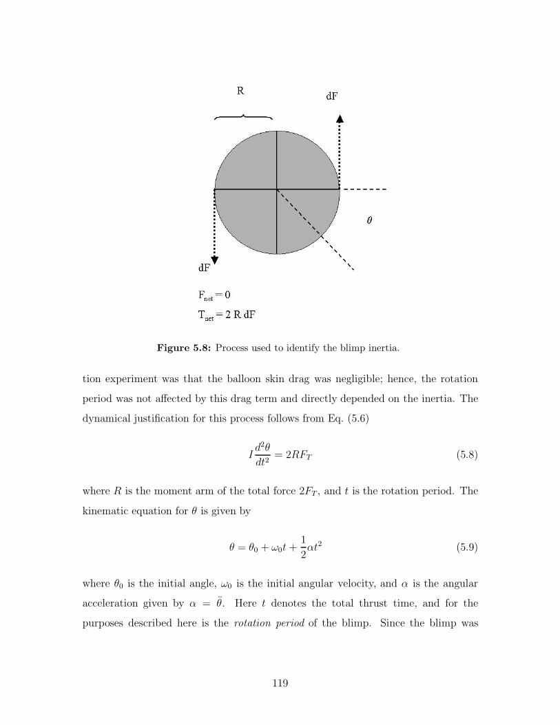
Figure 5.8: Process used to identify the blimp inertia.

tion experiment was that the balloon skin drag was negligible; hence, the rotation

period was not affected by this drag term and directly depended on the inertia. The

dynamical justification for this process follows from Eq. (5.6)

Id2θ

dt2= 2RFT (5.8)

where R is the moment arm of the total force 2FT , and t is the rotation period. The

kinematic equation for θ is given by

θ = θ0 + ω0t +1

2αt2 (5.9)

where θ0 is the initial angle, ω0 is the initial angular velocity, and α is the angular

acceleration given by α = θ. Here t denotes the total thrust time, and for the

purposes described here is the rotation period of the blimp. Since the blimp was

119

initially stationary, θ0 = 0 and ω0 = 0 and Eq. (5.9) simplifies to

α =2θ

t2(5.10)

Substituting this in Eq. (5.8) results in the expression

I =2RFT

α⇒ t2I =

R

θFT (5.11)

Recall that the moment arm R is known, the actuation force FT is known, and the

period of rotation can be measured; hence the inertia can be uniquely identified.

Here, only one rotation was evaluated, and so θ = 2π radians, a constant.

Numerous trials were done with different thrust values which resulted in different

rotation periods. The inertia was then found by least-squares. N measurements were

taken; defining the vector of times t2i as T ≡ [ t21 | t22 | . . . | t2N ]T and the vector of

different thrusts F ≡ [ FT,1 | FT,2 | . . . | FT,N ]T then Eq. (5.11) can be expressed as

T I =R

θF (5.12)

and the inertia can be solved explicitly by least squares as

I =R

θ(T T T )−1 T T F (5.13)

where I denotes the least squares estimate of the inertia, which was found to be

1.55 Kg-m2.

Drag Coefficient

The drag coefficient was calculated by flying the blimp at a constant velocity. At this

point, the thrust of the blimp was equal in magnitude to the drag force, so the drag

can be found by equating the two

D =1

2ρCDAv2 ≡ FT ⇒ CD =

2FT

Aρv2(5.14)

120

Table 5.2: Blimp and Controller Characteristics

Symbol Definition Value

I Inertia 1.55 kg − m2

M Mass 10 KgC Drag Coefficient 0.5

Kp,v Velocity P gain 0.75Kp,z Altitude P gain 28.65Kd,z Altitude D gain 68.75Kp,h Heading P gain 0.004Kd,h Heading D gain 0.016cf Thrust2Servo Slope (forward) 55.15cb Thrust2Servo Slope (backward) 45.15df Thrust2Servo Intercept (forward) 6db Thrust2Servo Intercept (backward) 5

Since the thrust FT and velocity v of the blimp were both known, the drag coefficient

was found by isolating it as in Eq. (5.14). Since the linear model was used for the

controllers, the coefficient for the linearized drag C had to be expressed in terms

of the drag coefficient CD (C ≡ ρCDAv0). The value of the drag coefficient C was

found to be approximately 0.5, for CD ≈ .12. Note that the value CD fell within the

accepted range of 0.1 − 4 for spherical objects [4].

A summary table of the main parameters of the blimp is shown in Table 5.2. The

table also includes the controller gains introduced in the next section.

5.4 Blimp Control

Three control loops were developed for the blimp for velocity, altitude, and heading

control [47]. These controllers are introduced in the next sections. The transmis-

sion delays, τ , in the physical system were approximated using a 2nd order Pade

approximation

e−τs ≈1 − τs

2+ (τs)2

12

1 + τs2

+ (τs)2

12

(5.15)

121

5.4.1 Velocity Control Loop

The transfer function from the commanded thrust to the velocity with the delay (τv)

included is given by

Gv(s) =V (s)

FT (s)=

e−τvs

Ms + C(5.16)

The thrust command is given by a proportional control via a combination of a refer-

ence state and an error term

FT ≡ Cvref + Kp,vverr (5.17)

where vref is the desired reference velocity and Kp,v is the proportional gain on the

velocity error verr = v − vref . This reference state is added so that even when the

velocity error is zero, a thrust command is still provided to actuate against the effect

of the drag and maintain the current velocity. A steady-state error in the velocity will

result if the incorrect drag coefficient is found. A root locus for the velocity control

loop is shown in Figure 5.9 with a delay of approximately 0.5 seconds in the velocity

loop.

5.4.2 Altitude Control Loop

The altitude control loop uses the tilt angle γ of the servos to increase or decrease

the altitude of the blimp. While the relation involves a nonlinear sinx term, this

term is linearized using the familiar small angle approximation of sin x ≈ x. This

is justified by the fact that for the scope of the current heterogeneous testbed, the

blimp is generally operated at constant altitude, and is not required to change altitude

frequently; furthermore, these altitude changes are small (generally not larger than

0.5 meters) and for reasonable damped responses, the control request for the angle

γ does not exceed 30◦. While these requests exceeded the assumptions for the small

angle approximations, they were generally infrequent; the nominal requests were on

the order of 10◦ − 15◦ which did satisfy the assumptions of the approximation. The

122

−7 −6 −5 −4 −3 −2 −1 0 1 2 3 4−2.5

−2

−1.5

−1

−0.5

0

0.5

1

1.5

2

2.5

Imag

Axi

s

Real Axis

Velocity Root Locus with Delay

Figure 5.9: Root locus for closed loop velocity control

equations of motion for the altitude motion given in Eq. (5.5) then become

Md2z

dt2≈ FTγ − C

dz

dt(5.18)

The transfer function with a delay (τz) of approximately 1 second (due to the actua-

tion and the servos being tilted correctly) then becomes

Gz(s) =Z(s)

γ(s)=

e−τzsFT

Ms2 + Cs(5.19)

To control this second order plant, the altitude error, zerr = z − zref and altitude

error rate zerr = d (z − zref ) /dt are used to create a PD compensator of the form

Gz(s) =Kp,z + Kd,zs

FT(5.20)

123

−8 −6 −4 −2 0 2 4−2.5

−2

−1.5

−1

−0.5

0

0.5

1

1.5

2

2.5

Imag

Axi

s

Real Axis

Altitude Root Locus with Delay

Figure 5.10: Root locus for closed loop altitude control.

where Kp, z is the proportional gain on the altitude error, and Kd, z is the derivative

gain on the altitude error rate. The root locus of the altitude control loop is shown

in Figure 5.10.

5.4.3 Heading Control Loop

The blimp controls heading by applying a differential thrust: +dF on one motor and

−dF on the other. The net thrust will remain the same at FT , but there will be

a net torque T , given by T = 2 R dF , where, as before, R is the moment arm to

the motors. The length of this moment arm was given in Section 5.3 as 50 cm. The

transfer function from the torque to the heading is given by

Gh(s) =Θ(s)

T (s)=

e−τhs

Is2 + CDrots(5.21)

124

−10 −8 −6 −4 −2 0 2 4−3

−2

−1

0

1

2

3Heading Root Locust with Delay

Real Axis

Imag

Axi

s

Figure 5.11: Root locus for closed loop heading control.

where τh is the time delay in the heading response. The heading error herr = h−hdes

and heading error rate herr = d (h − hdes) /dt and are used in the PD compensator

T = Kp,hherr + Kd,hherr (5.22)

The root locus is shown in Figure 5.11.

5.5 Experimental Results

This section presents results that demonstrate the effectiveness of the closed loop

control of velocity, altitude, and heading. Each loop closure is presented individually

and all three loops are then closed in a circle flight demonstration.

125

5.5.1 Closed Loop Velocity Control

Recall that a proportional controller was used for the velocity loop; closed loop control

of velocity was demonstrated by step changes in the requested velocity of the blimp.

A typical response of the velocity control system is shown in Figure 5.12 in which the

blimp started stationary (neutrally buoyant), and a reference speed of 0.4 m/s was

commanded (hence simulating a 0.4 m/s step input). The velocity control system was

designed to be slightly over damped (as seen from root locus), and does not achieve

the reference velocity with zero error. Note, however, that this error is very small, on

the order of 2.5 cm/s.

The velocity controller is extremely dependent on the correct value of the drag

coefficient which was calculated with an assumed wetted area of the balloon. During

the course of a test, both the shape and area of the balloon could change primarily

due to helium leaks. Thus, the small errors in steady-state velocity were attributed to

using a controller designed for a certain type of drag coefficient which varied through

the course of the experiments.

5.5.2 Closed Loop Altitude Control

Closed loop control of altitude is demonstrated by step changes in the requested

altitude of the blimp. Here, the altitude of the blimp initially exhibited a large

overshoot which was damped to within 8 cm in approximately 15 seconds. This time

constant was acceptable for the requirements for the blimp, but the overshoot is quite

dramatic. This test was done while the blimp in forward motion, approximately 0.4

m/s.

5.5.3 Closed Loop Heading Control

The heading loop of the blimp was also closed. Figure 5.14 shows a step change of 90◦

from a heading of 200◦ to 110◦, flying at a velocity of approximately 0.4 m/s. This

was a very large heading change for the blimp, especially complicated by the almost

1-second time delay in the system. While the blimp was not specifically designed to

126

0 5 10 15 20 25 30 35 40 450

0.05

0.1

0.15

0.2

0.25

0.3

0.35

0.4

0.45

0.5

Time

Vel

ocity

, m/s

ec

Velocity Control Loop

VV

des

Figure 5.12: Closed loop velocity control

turn so aggressively, this represents an extreme case that demonstrates the successful

loop closure of the heading loop.

The overall maneuver takes approximately 12 seconds and the figure shows a

smooth transition from the original heading to the final heading. There is a steady-

state error from 45 seconds onwards, when the blimp has reached the vicinity of its

target heading. The average steady-state error from 45 to 52.5 seconds is approx-

imately 2-3 degrees. While this error could be decreased by varying the controller

gains in an ideal system, blimp stability became the primary concern when these

changes were made. Note however that this error is acceptable for the distances in

which the blimp will be operating, as they will be on the order of 20-30 meters, and

a cross-track error due to this heading difference is on the order of 1.5 meters, which

will be corrected continuously by an improved waypoint controller. Figure 5.15 shows

the heading controller tracking a 250◦ heading. The blimp actual heading appears

127

0 5 10 15 20 25 30 35 40 45−0.5

−0.4

−0.3

−0.2

−0.1

0

0.1

0.2Altitude Control Loop

Time

Alti

tude

, met

ers

zzdes

Figure 5.13: Closed loop altitude control

very oscillatory due to a pitching motion that was induced by a misaligned center of

mass. This motion caused the blimp to oscillate with a period of approximately 3 sec-

onds. The key point is that the pitch angle was sufficiently large to invalidate the key

assumption of blimp level flight used in Eq. (5.1). Hence, the heading was estimated

to be changing more quickly than it actually was. The heading controller responded

quickly to these oscillations, and maintained the blimp heading within −5.5◦ and +4◦

of the requested heading, as seen in Figure 5.16. The closed loop response to step

changes in heading is shown in Figure 5.16

5.5.4 Circular Flight

This section shows the blimp successfully flying a circle at a constant altitude and

velocity. This demonstrates that the three control loops on the blimp were closed

successfully. The circle was discretized by a set of fixed heading changes that were

128

25 30 35 40 45 50

100

120

140

160

180

200

Heading Loop − Gain = 0.07, Zero at −0.25i

Time

Hea

ding

(de

g)

DesiredActual

Figure 5.14: Blimp response to a 90◦ degree step change in heading

passed from a planner to the blimp heading controller. These heading changes were

successfully tracked by the blimp for the duration of the test, which was approximately

10 minutes. A representative flight test is shown in Figure 5.17. Note the slightly

pear-dropped shape of the circle; this was caused by currents in the air conditioning

system of the test area that the blimp could not account for, since it was not doing

station keeping about the center of the circle. Hence the blimp did not try to maintain

its absolute position within a certain radius from the center of the circle; rather the

objective was to track the heading changes at a constant altitude and velocity. Note

that the blimp deviations about the reference altitude never exceeded 8cm. Even

though this figure shows approximately the first two minutes, this is representative

of the remainder of the flight.

129

0 5 10 15 20 25 30 35 40 45200

210

220

230

240

250

260

270

280Heading Control Loop

Time

Hea

ding

, deg

rees

hh

des

Figure 5.15: Closed loop heading control

0 5 10 15 20 25 30 35 40 45−10

−8

−6

−4

−2

0

2

4

6

8

10Heading Control Loop: Error

Time

Hea

ding

err

or, d

egre

es

Heading error

Figure 5.16: Closed loop heading error.

130

5 10 150

2

4

6

8

10

12

Y a

xis

X axis

Bird’s eye view of the circle

40 50 60 70 80 90 100 110 120

−0.9

−0.6

−0.3

0

Time, seconds

Z, m

eter

s

Z vs. timeZZ desired

Figure 5.17: Blimp flying an autonomous circle

5.6 Blimp-Rover Experiments

This section presents some results that were obtained with the rover and the blimp

acting in a cooperative fashion. Here, the blimp was launched simultaneously with

the rover; the rover had an initial situational awareness of the environment that was

updated by the blimp when it flew in the vicinity of the obstacle. This example

is representative of the scenarios that were shown with the previous algorithms of

the RRHTA and RRHTAR. Here, the blimp acting as a recon vehicle provides the

information to the rover, which can then include it in the task assignment and path

planning algorithms. Furthermore, by overflying the obstacles, the blimp can reduce

the uncertainty regarding the identity of those obstacles.

In this scenario, the blimp started at (6.5,1) and the rover started at (10,0). The

131

0 5 10 150

2

4

6

8

10

12

14

16

18

20

22

X [m]

Y [m

]

C

B

A

Blimp

Rover

Figure 5.18: Blimp-rover experiment

rover had an initial target map composed of vehicles A and B. It did not know of

the existence of target C. The blimp began flying approximately 10 seconds after the

rover, and was assigned by the higher level planner to “explore” the environment by

giving it reference velocity and heading commands.

Since the original rover assignment was composed of targets A and B, Figure 5.18

shows that after visiting target A, the rover originally changes heading to visit target

B. However, 5 seconds after the rover visited target A, the blimp discovered target B

and sent this new target information to the central planner, which then updated the

rover’s target list. The rover then was reassigned to visit target C, and this can be

seen in the figure, with the rover changing heading to visit target C first, and finally

visiting target B.

132

This test demonstrated a truly cooperative behavior between two heterogeneous

vehicles; while implemented in a decoupled fashion, the blimp was used to explore

the environment, while the truck was used to strike the targets. From a hardware

perspective, this series of tests successfully demonstrated the integration of the two

vehicles under one central planner.

5.7 Conclusion

This chapter has presented the design and development of an autonomous blimp. Sec-

tion 5.2 presented the elements of the hardware testbed and Section 5.3 introduced

the blimp design and development. Section 5.4 presented the control algorithms

developed for lower-level control of the vehicle. Sections 5.5 and 5.6 presented exper-

imental results for the blimp and blimp-rover combinations. The blimp currently has

sufficient payload capability to lift an additional small sensor, such as a camera, that

could be used to perform actual reconnaissance missions.

133

Chapter 6

Conclusions and Future Work

6.1 Conclusions

This thesis has emphasized the robustness to uncertainty of higher-level decision mak-

ing command and control. Specifically, robust formulations have been presented for

various decision-making algorithms, to hedge against worst-case realizations of target

information. These formulations have demonstrated successful protection without

incurring significant losses in performance.

Chapter 2 presented several common forms of robust optimization presented in

literature; a new formulation (Modified Soyster) was introduced that both maintains

computational tractability and successfully protects the optimization from the worst-

case parameter information, while maintaining an acceptable loss of performance. The

chapter also demonstrated strong relations between these various formulations when

the uncertainty impacted the objective coefficients. Finally, the Modified Soyster was

compared to the Bertsimas-Sim algorithm in an integer portfolio optimization, and

both successfully protected against worst-case realizations while at an acceptable loss

in performance.

Chapter 3 presented a robust Weapon Task Assignment (RWTA) formulation that

hedges against the worst-case. A modification was made to incorporate reconnais-

sance as a task that can be assigned to reduce the uncertainty in the environment. A

full reconnaissance-strike problem was then posed as a mixed-integer linear program.

135

Several numerical examples were given to demonstrate the advantage of solving this

joint assignment problem simultaneously rather than using a decoupled approach.

Chapter 4 presented a modification of the RHTA [1] to make it robust to un-

certainty by creating the RRHTA, and extended the notion of reconnaissance to

this assignment (creating the RRHTAR). This specific extension emphasized that

vehicle-task assignment in the RHTA relies critically on both the physical distances

and uncertainty in the problem formulation. Results were demonstrated showing the

advantage of incorporating reconnaissance in a RHTA-like framework.

Finally, Chapter 5 introduced the blimp as a new vehicle that makes the existing

testbed truly heterogeneous. The control algorithms for the blimp were demonstrated,

and a truck-blimp experiment was shown.

6.2 Future Work

The study of higher-level command and control systems remains a crucial area of

research. More specifically, analyzing these systems from a control-theoretic perspec-

tive should give great insight into issues that still need to be fully understood, such

as stability in the presence of time delays and communication bandwidth limitations

among the different control levels. This thesis has primarily emphasized the per-

formance of decision-making under uncertainty, and has developed tools that make

the objective robust to the uncertainty. There are still some fundamental research

questions that need to be addressed and future work should focus on: i) including

robust constraint satisfaction, and ii) incorporating more sophisticated representa-

tions of the battle dynamics. While robust performance is an important part of this

problem, robust constraint satisfaction, i.e., maintaining feasibility in the presence

of uncertainty, is also crucial. This problem is important since planning without un-

certainty could lead to missions that are not physically realizable. While this thesis

has analyzed optimizations with rather simple and deterministic constraints, more

sophisticated and in general uncertain constraints (such as incorporating attrition in

multi-stage optimizations) should be included. The overall mission should be robust

136

in the presence of this uncertainty, and the tools developed in this thesis should be

extended to deal with the uncertain constraints.

Battle dynamics should also be modified to incorporate more representative sensor

models and uncertainties. For example, while this thesis emphasized the presence of

information uncertainty in the environment, it did not consider adversarial models

for the enemy or attrition models for the strike vehicles. Incorporating these models

in more sophisticated battlefield simulations will address key research questions while

improving the realism of battlefield dynamics, thereby reducing the gap between the

abstract development and applicability of the theory.

137

Bibliography

[1] M. Alighanbari, “Task Assignment Algorithms for Teams of UAVs in Dynamic

Environments.” S. M. Thesis, June 2004.

[2] M. Alighanbari, L. F. Bertuccelli, and J. P. How. “Filter-Embedded UAV Assign-

ment Algorithms for Dynamic Environments.” AIAA GNC, 2004.

[3] ActivMedia Robotics. “Pioneer Operations Manual,” January 2003.

http://robots.activmedia.com

[4] J. Anderson. “Fundamentals of Aerodynamics.” McGraw-Hill. New York, 1991.

[5] ArcSecond. “Constellation 3D-i Error Budget and Specifications.” June, 2002.

http://www.arcsecond.com

[6] J. S. Bellingham, M. J. Tillerson, A. G. Richards, J. P. How, “Multi-Task As-

signment and Path Planning for Cooperating UAVs,” Conference on Cooperative

Control and Optimization, Nov. 2001.

[7] A. Ben-Tal, T. Margalit, and A. Nemirovski. “Robust Modeling of Multi-Stage

Portfolio Problems” In: H. Frenk, K. Roos, T. Terlaky, and S. Zhang. (Eds.) ”High-

Performance Optimization”, Kluwer Academic Publishers, 303-328. 2000.

[8] A. Ben-Tal and A. Nemirovski, “Robust Solutions of Uncertain Linear Programs”

Operations Research Letters, Vol. 25, pp. 1-13.

[9] A. Ben-Tal and A. Nemirovski, “Robust Solutions of Linear Programming Prob-

lems Contaminated with Uncertain Data” Matematical Programming, Vol. 88,

pp. 411-424.

139

[10] D. Bertsimas and J. Tsitsiklis, “Introduction to Linear Optimization,” Athena

Scientific 1997.

[11] D. Bertsimas and M. Sim, “Robust Discrete Optimization and Network Flows,”

submitted to Operations Research Letters, 2002.

[12] D. Bertsimas and M. Sim, “Price of Robustness,” submitted to Mathematical

Programming, 2002.

[13] L. F. Bertuccelli, M. Alighanbari, and J. P. How. “Robust Planning for Coupled

Cooperative UAV Missions,”, submitted to IEEE CDC 2004.

[14] J. R. Birge and F. Louveaux, “Introduction to Stochastic Programming”,

Springer-Verlag, 1997.

[15] J. A. Castellanos, J. Neira, and J. D. Tardos. “Multisensor Fusion for Simulta-

neous Localization and Map Building.” IEEE Transactions on Robotics and Au-

tomation, Vol. 17(6), 2001.

[16] P. Chandler, M. Pachter, D. Swaroop, J. Fowler, et al. “Complexity in UAV

cooperative control,” IEEE ACC 2002, pp. 1831-1836.

[17] G. B. Dantzig and G. Infanger. “Multi-Stage Stochastic Linear Programs for

Portfolio Optimization.” Annals of Operations Research, Vol. 45, pp. 59-76. 1993.

[18] L. El-Ghaoui and H. Lebret. “Robust Solutions to Least-Square Problems to Un-

certain Data Matrices,” SIAM Journal of Matrix Analy. and Appl., (18), pp. 1035–

1064.

[19] H. Fourer, D. M. Gay, and B. W. Kernighan. AMPL: A Modeling Language for

Mathematical Programming. The Scientific Press, 1993.

[20] A. Gelb, “Applied Optimal Estimation”, MIT Press, 1974.

[21] B. Grocholsky, A. Makarenko, and H. Durrant-Whyte. “Information-Theoretic

Coordinated Control of Multiple Sensor Platforms.” IEEE International Conference

on Robotics and Automation September 2003, Taipei, Taiwan.

140

[22] P. Hosein, and M. Athans. “The Dynamic Weapon Target Assignment Problem.”

Proc. of Symposium on C2 Research, Washington, D.C. 1989.

[23] Honeywell. “HMR2300 Smart Digital Magnetometer Product Information.”

http://www.honeywell.com

[24] D. R .Jacques and R. L Leblanc. “Effectiveness Analysis for Wide Area Search

Munitions.” AIAA, available at http://eewww.ecn.ohio-state.edu/ passino.

[25] P. Kouvelis and G. Yu, “Robust Discrete Optimization and Its Applications,”

Kluwer Academic Publishers, 1996.

[26] P. Krokhmal, R. Murphey, P. Pardalos, S. Uryasev, and G. Zrazhevsky. “Robust

Decision Making: Addressing Uncertainties in Distributions”, In: S. Butenko et

al. (Eds.) ”Cooperative Control: Models, Applications and Algorithms”, Kluwer

Academic Publishers, 165-185. 2003.

[27] P. Krokhmal, J. Palmquist, and S. Uryasev. “Portfolio Optimization with Con-

ditional Value-At-Risk Objective and Constraints.” The Journal of Risk, Vol. 4,

No. 2, 2002.

[28] Y. Kuwata. “Real-Time Trajectory Design for Unmanned Aerial Vehicles using

Receding Horizon Control,“S.M. Thesis,” 2003.

[29] H. Markowitz. “Portfolio Selection”, The Journal of Finance, (7) No. 1, pp. 77-

91, 1952.

[30] W. M. McEneaney and B. Fitzpatrick, “Control for UAV Operations Under

Imperfect Information,” AIAA, 2002–3418.

[31] J. M. Mulvey, R. J. Vanderbei, and S. A. Zenios. “Robust Optimization of Large-

Scale Systems,” Operations Research (43), pp. 264-281, 1995.

[32] R. A. Murphey, “An Approximate Algorithm For A Weapon Target Assignment

Stochastic Program,” in Approximation and Complexity in Numerical Optimiza-

141

tion: Continuous and Discrete Problems, P. M. Pardalos ed., Kluwer Academic

Publishers, 1999.

[33] R. A. Murphey, “Target-Based Weapon Target Assignment Problems,” in Non-

linear Assignment Problems: Algorithms and Applications, P. M. Pardalos and

L. S. Pitsoulis eds., Kluwer Academic Publishers, 2000.

[34] J. Neira and J. D. Tardos. “Data Association in Stochastic Mapping Using

the Joint Compatibility Test.” IEEE Transactions on Robotics and Automation.

Vol. 17(6), 2001.

[35] O. of the Secretary of Defense, “Unmanned Aerial Vehicles Roadmap,” tech.

rep., December 2002. http://www.acq.osd.mil/usd/uav roadmap.pdf

[36] Y. Oshman and P. Davidson. “Optimization of Observer Trajectories for

Bearings-Only Target Localization.” IEEE Trans. on Aerospace and Electronic Sys-

tems, Vol. 35(3), 1999.

[37] D. Pachamanova, “A Robust Optimization Approach to Finance,” Ph.D. Thesis,

June 2002.

[38] R. T .Rockafellar, and S. Uryasev. “Optimization of Conditional Value at Risk,”

available at http://www.ise.ufl.edu/uryasev, 1999.

[39] F. Schweppe. Uncertain Dynamical Systems, Prentice-Hall, 1973.

[40] C. Schumacher, P. R. Chandler, and S. R. Rasmussen. “Task Allocation for Wide

Area Search Munitions.” ACC, 2002.

[41] A. L. Soyster, “Convex Programming with Set-Inclusive Constraints and Ap-

plications to Inexact Linear Programming,” Operations Research, 1973, pp. 1154–

1157.

[42] J. E. Tierno and A. Khalak , “Frequency Domain Control Synthesis for Dis-

counted Markov Decision Processes,” IEE European Control Conference. Cam-

bridge, UK ,Sept. 2003.

142

[43] USAF Board, “UAV Technologies and Combat operations,” Tech. Rep. Tech.

Tep. SAB-TR-96-01, November 1996.

[44] http://www.af.mil

[45] C. von Clausewitz. On War. Dummlers Verlag, Berlin, 1832.

[46] S. Waslander. “Blimp Mass Budget,” MIT Internal Report, 2004.

[47] S. Waslander and J. McRae. “Blimp Summary Report,” MIT Internal Report,

2004.

[48] S.-S. Zhu, D. Li, and S.-Y. Wang, “Risk Control Over Bankruptcy in Dynamic

Portfolio Selection: A Generalized Mean-Variance Formulation,” IEEE Transac-

tions on Automatic Control, Vol. 49, No. 3, pp. 447–457.

143

Robust Planning for Heterogeneous UAVs in Uncertain ... · Bachelor of Science in Aeronautical and...

Documents

Transcript of Robust Planning for Heterogeneous UAVs in Uncertain ... · Bachelor of Science in Aeronautical and...