Robust PID Control of the QuadrotorHelicopter ?

R.A. Garcıa, F.R. Rubio and M.G. Ortega

Dpto Ing Sistemas y Automatica. Universidad de sevilla, EscuelaTecnica Superior de Ingenierıa, 41092, Sevilla, Spain.

{ramongr, rubio, mortega}@us.es

Abstract: In this paper a robust PID control strategy via affine parametrization is designed foran multivariable nonlinear unmanned aerial vehicle. The robustness of the controlled system isassured by using the H∞ norm of the weighted complementary sensitivity function. Simulationresults carried out using a complete nonlinear model are shown, wherein the performanceachieved with this control strategy is shown.

Keywords: PID, Robust control, UAV, Simulation, Model.

1. INTRODUCTION

Unmanned Aerial Vehicles, UAVs, are well advanced inrecent years, especially the quadrotor equipments. Theyare helicopters whose main feature is that they have fourcoplanar motors. Furthermore, as helicopter, it enablesa hover, allowing the testing of control techniques forstabilization and height regulation regardless of the dis-placement in the XY plane.

This kind of airship also requires continuous control action,because the system is unstable. The slightest change in anuncontrolled action from the engines can cause the systemleave the stable operating point.

A lot of researches have been carried out in a wide rangeof fields in control and robotics, such as computer visionfeedback, fusion sensor, and linear and nonlinear controlmethodologies to improve performance of this kind ofsystem.

Equations of movements for this kind of helicopter can befound in (Castillo et al (2007), Raffo et al (2008)). Theseequations can be used for the control of the helicopterby means of many control strategies, such as MPC, H∞,and PID, among others (Alexis et al (2011), Chen et al(2003,AIAA), Chen et al (2003)). Feedback informationcan be provided by inertial measurement units, GPS, oreven computer vision systems (Altug et al (2002)).

In this paper, a fixed-structure robust PIDs are used tocontrol both the attitude and the height of a quadrotorhelicopter. PIDs are very extended in industry due tothe possibility of experimental settings and the insightof their parameters tuning. Focusing on robust control,this control theory allows to consider uncertainties whichare not described in a nominal model, such as delays orvariations in certain values due to complex measurements.In Saeki (2006) can be found a work concerning robustPID design via LMIs.

? The authors want to thank the MICINN for funding this workthrough project DPI2010-19154.

In this work, the PID controllers have been synthesizedthrough affine parametrization. This methodology cancancel the stable-known dynamics of the system. Andfor the unknown dynamics and parameter uncertainty, arobust design using H∞ theory is implemented. By com-bining robust and affine approaches, PID controllers areobtained which guarantee functionality under uncertainconditions.

The remainder of the paper is organized as follows. Section2 describes the model of quadrotor used in this work. InSection 3, the controllers structure and its implementationare explained. Simulation results are presented in Section4, and finally the main conclusions are drawn in Section 5.

2. SYSTEM MODELING

A scheme of the system is presented in Fig. 1, whereindifferent forces and torques actuating on the quadrotor canbe observed. Basically, they are the followings: total force,F , roll torque, τφ, pitch toque, τθ, and yaw torque, τψ.However the actuators are four rotors represented by theirforces, fi. Therefore, the desired total force and torqueshave to be achieved by exerting some combination of fi asfollows:

F = f1 + f2 + f3 + f4

τφ = l · (f2 − f4) , τθ = l · (f3 − f1)

τψ =ktb· (f1 + f3 − f2 − f4),

(1)

where l is the distance from the center of rotation to therotors, kt is the drag coefficient of the motors and b is thethrust coefficient of the rotors. The following values havebeen considered for this work from a particular quadrotor:

kt = 1.06 · 10−8Nm2(τψ = ktω

2)

b = 5.8 · 10−7Ns2(f = bω2

).

(2)

The aim is to control the height and the stabilization ofthe UAV simultaneously. Next, the nonlinear equations of

IFAC Conference on Advances in PID Control PID'12 Brescia (Italy), March 28-30, 2012 WeC2.5

Fig. 1. Model scheme: Main forces and torques

motion for the height, z and for these three angles areshown, wherein the roll, pitch and yaw Euler angles arenoted as φ, θ and ψ respectively (Raffo et al (2010)), (Raffoet al (2008)).

• Equation for the height expressed with respect to aninertial frame W:

z = −g +1

m(cos θ cosφ)F +

Azm, (3)

being Az a disturbance acting on the Z axis. c

• Equations for the three Euler angles:

I(η)η + C(η, η)η = τη + τηdist . (4)

Being I(η) inner matrix, η Euler angles, C Coriolismatrix, τη torques applied and τηdist disturbancetorques.

τη =

[τφτθτψ

](5)

I(η) =

[i11 i12 i13i21 i22 i23i31 i32 i33

](6)

i11 = Ixx, i13 = −Ixx sin θ

i12 = i21 = 0

i22 = Iyy cos2 φ+ Izz sin

2 φ

i23 = (Iyy − Izz) cosφ sinφ cos θ

i31 = −Ixx sin θ, i32 = (Iyy − Izz) cosφ sinφ cos θ

i33 = Ixx sin2 θ + Iyy sin

2 φ cos2 θ + Izz cos2 φ cos2 θ

(7)

C(η, η) =

[c11 c12 c13c21 c22 c23c31 c32 c33

](8)

c11 = 0

c12 = (Iyy − Izz)(θ cosφ sinφ+ ψ sin2φ cos θ)

+(Izz − Iyy)ψ cos2φ cos θ − Ixxψ cos θ

c13 = (Izz − Iyy)ψ cosφ sinφ cos2θ

c21 = (Izz − Iyy)(θ cosφ sinφ+ ψ sin2φ cos θ)

+(Iyy − Izz)ψ cos2φ cos θ + Ixxψ cos θ

c22 = (Izz − Iyy)φ cosφ sinφ

c23 = −Ixxψ sin θ cos θ + Iyyψ sin2φ cos θ sin θ

+Izzψ cos2φ sin θ cos θ

c31 = (Iyy − Izz)ψ cos2θ sinφ cosφ− Izz θ cos θ

c32 = (Izz − Iyy)(θ cosφ sinφ sin θ + φ sin2φ cos θ)

+(Iyy − Izz)φ cos2φ cos θ + Ixxψ sinφ cos θ

−Iyyψ sin2φ sin θ cos θ − Izzψ cos

2φ sin θ cos θ

c33 = (Iyy − Izz)φ cosφ sinφ cos2θ − Ixxθ sin

2φ cos θ sin θ

−Izz θ cos2 φ cos θ sin θ + Ixxθ cos θ sin θ

(9)

These equations describe the system behavior in all itsworkspace. However, in this paper a hovering flight isconsidered, and therefore, the desired equilibrium pointconsists in keeping null values for the Euler angles, at leastfor the pitch and roll angles. Keeping in mind this fact,the original model can be simplified, yielding the followinglinear expressions:

z =F

m, φ =

τφIxx

, θ =τθIyy

, ψ =τψIzz

(10)

The values of the mass, the length from the center ofthe mass to the rotor and the inertias considered can beobserved below, they would be obtained experimentally:

m = 2.24 kg, l = 0.332 m, Ixx = 0.038425 kgm2

Iyy = 0.038421 kgm2, Izz = 0.061547 kgm2(11)

Then the plant without considering the rotors dynamics isgiven by:

Gi(s) =Ki

s2, {i = z, φ, θ, ψ}. (12)

These transfer functions represent a simplified linearmodel obtained from movement equations. Neverthelessin this model, neither the delays from communication(of about 20 ms) due to the motors driver nor motorsdynamics are considered. Besides, some coupling is notconsidered either, which appears when the helicopter isworking far from the desired equilibrium points. All thesefacts will be dealt as a system uncertainties.

3. CONTROLLER DESIGN

Four controllers are needed, one for the height and onefor each angle. A PID based on affine parametrization isgoing to be presented. This classic controller, C(s), hasthe following structure:

CPID(s) = KPTITDs

2 + TIs+ 1

TIs (τDs+ 1), (13)

Based on an affine parametrization, the controller can beexpressed in the following form (Goodwin et al (2000):

C(s) =Q(s)

1−Q(s)G(s), (14)

IFAC Conference on Advances in PID Control PID'12 Brescia (Italy), March 28-30, 2012 WeC2.5

where the transfer function Q(s) acts as parameter whichmay cancel the stable dynamics of the plant. Therefore,Q(s) can be expressed as follows:

Q(s) = FQ(s)G−1(s), (15)

where FQ(s) is chosen to satisfy some constraints (Good-win et al (2000)).

In the case under consideration,

G−1(s) =s2

K. (16)

It is known that Q(s) must be proper, which yields FQ(s)needs to have relative degree 2. In addition, since a specificPID structure for the controller is desired, and taking intoaccount that input sensitivity transfer function

Sio(s) = [1−Q(s)G0(s)]G0(s) (17)

must have a zero at the origin in order to be able to rejectsustained disturbances, the following general expressionfor FQ(s) is proposed:

FQ(s) =α2s

2 + α1s+ 1

α4s4 + α3s3 + α2s2 + α1s+ 1(18)

By substituting this expression of FQ(s) into (15) and (14),and after some manipulations, the following controller isobtained:

C(s) =α2s

2 + α1s+ 1

α3Ks(α4

α3s+ 1)

(19)

By comparing the preceding expression with Eq. (13), itis easy to obtain the following correlations:

KP =α1

α3K, TI = α1 , TD =

α2

α1, τD =

α4

α3(20)

In this work, the following conditions have been taken intoaccount for the controllers design. On the one hand, inorder to optimize the disturbances rejection, the followingconstraints has been imposed:

TI = 4TD → α2 =α21

4(21)

On the other hand, the time constant of the high frequencypole is chosen as follows:

τD =TD10→ α4 =

α2

α1

10α3 (22)

Under these constraints, the controllers have two parame-ters to adjust, α1 and α3. Their adjustment will be carriedout in order to provided robustness to the controlled sys-tem.

For the design of a robust controller, first the followinguncertain plant is considered:

G∗i (s) =K∗i

s2(τms+ 1)e−Ls (23)

In this uncertain plant, structural and parametric uncer-tainties with respect to the nominal model are included.τm represents the motor time constant, whose value hasbeen estimated about 0.1 seconds, and L is the delay dueto the ESC (Electronic Speed Controller) driver, whose

Fig. 2. Uncertainties in Z coordinate and estimated bound

Fig. 3. Uncertainties in Roll coordinate and estimatedbound

value is around 20 ms. In addition, a gain variation of a±25% is also considered.

Once the uncertain plants have been selected, the multi-plicative uncertainty with respect the nominal model canbe estimated as follows:

|Emi(jω)| = |G∗i (jω)−Gi(jω)||Gi(jω)|

, (24)

The modulus of the output multiplicative uncertainty canbe upper bounded by the modulus of a stable weightingfunction Wi(s). Both the estimated multiplicative uncer-tainty and the designed weighting function are depicted inFigs. 2 and 3 for the case of the height and the roll anglerespectively. The ones for the remaining Euler angles arevery similar to the roll angle case. It should be highlightedthe fact that the modulus of the weighting function growsat high frequencies, which is due to the fact that theuncertain models do not represent the real plant at thesefrequencies.

It is well-known (Sigurd (2005)) that to achieve a robustH∞ controller, it is necessary the inverse of the multiplica-tive uncertainty bound has to be an upper bound for thecomplementary sensitivity transfer function Ti(s)

IFAC Conference on Advances in PID Control PID'12 Brescia (Italy), March 28-30, 2012 WeC2.5

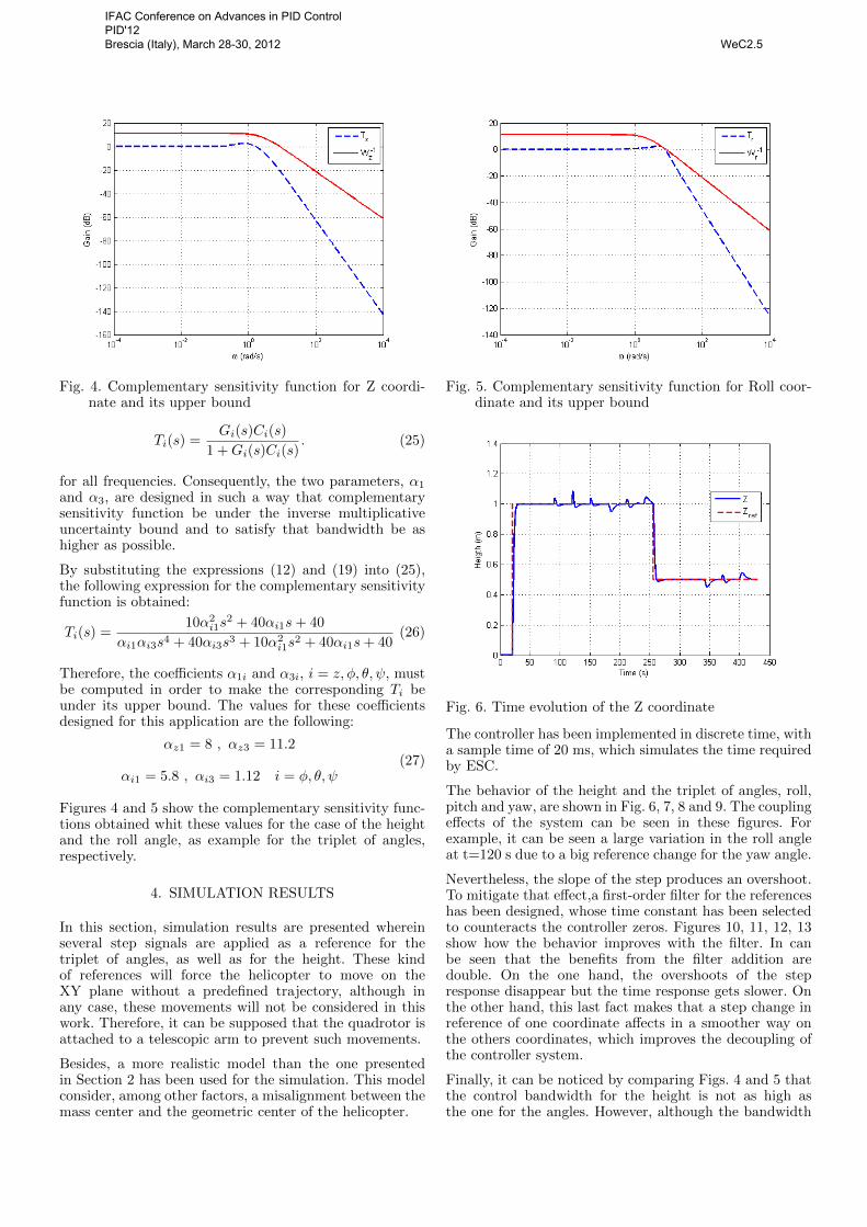
Fig. 4. Complementary sensitivity function for Z coordi-nate and its upper bound

Ti(s) =Gi(s)Ci(s)

1 +Gi(s)Ci(s). (25)

for all frequencies. Consequently, the two parameters, α1

and α3, are designed in such a way that complementarysensitivity function be under the inverse multiplicativeuncertainty bound and to satisfy that bandwidth be ashigher as possible.

By substituting the expressions (12) and (19) into (25),the following expression for the complementary sensitivityfunction is obtained:

Ti(s) =10α2

i1s2 + 40αi1s+ 40

αi1αi3s4 + 40αi3s3 + 10α2i1s

2 + 40αi1s+ 40(26)

Therefore, the coefficients α1i and α3i, i = z, φ, θ, ψ, mustbe computed in order to make the corresponding Ti beunder its upper bound. The values for these coefficientsdesigned for this application are the following:

αz1 = 8 , αz3 = 11.2

αi1 = 5.8 , αi3 = 1.12 i = φ, θ, ψ(27)

Figures 4 and 5 show the complementary sensitivity func-tions obtained whit these values for the case of the heightand the roll angle, as example for the triplet of angles,respectively.

4. SIMULATION RESULTS

In this section, simulation results are presented whereinseveral step signals are applied as a reference for thetriplet of angles, as well as for the height. These kindof references will force the helicopter to move on theXY plane without a predefined trajectory, although inany case, these movements will not be considered in thiswork. Therefore, it can be supposed that the quadrotor isattached to a telescopic arm to prevent such movements.

Besides, a more realistic model than the one presentedin Section 2 has been used for the simulation. This modelconsider, among other factors, a misalignment between themass center and the geometric center of the helicopter.

Fig. 5. Complementary sensitivity function for Roll coor-dinate and its upper bound

Fig. 6. Time evolution of the Z coordinate

The controller has been implemented in discrete time, witha sample time of 20 ms, which simulates the time requiredby ESC.

The behavior of the height and the triplet of angles, roll,pitch and yaw, are shown in Fig. 6, 7, 8 and 9. The couplingeffects of the system can be seen in these figures. Forexample, it can be seen a large variation in the roll angleat t=120 s due to a big reference change for the yaw angle.

Nevertheless, the slope of the step produces an overshoot.To mitigate that effect,a first-order filter for the referenceshas been designed, whose time constant has been selectedto counteracts the controller zeros. Figures 10, 11, 12, 13show how the behavior improves with the filter. In canbe seen that the benefits from the filter addition aredouble. On the one hand, the overshoots of the stepresponse disappear but the time response gets slower. Onthe other hand, this last fact makes that a step change inreference of one coordinate affects in a smoother way onthe others coordinates, which improves the decoupling ofthe controller system.

Finally, it can be noticed by comparing Figs. 4 and 5 thatthe control bandwidth for the height is not as high asthe one for the angles. However, although the bandwidth

IFAC Conference on Advances in PID Control PID'12 Brescia (Italy), March 28-30, 2012 WeC2.5

Fig. 7. Time evolution of the Roll angle

Fig. 8. Time evolution of the Pitch angle

Fig. 9. time evolution of the Yaw angle

control for the z coordinate may be increased, this factmay cause undesirable effects due to the coupling. As forexample, Figs. 14 and 15 show the behavior of the Z androll coordinates for the case of the same control bandwidthfor all coordinates, which is achieved by selecting thesame values for αz1 and αz3 than the ones for αφ1 andαφ3 respectively. Obviously, the control of the height gets

Fig. 10. Time evolution of the Z coordinate with filteredreference

Fig. 11. Time evolution of the Roll angle with filteredreference

Fig. 12. Time evolution of the Pitch angle with filteredreference

IFAC Conference on Advances in PID Control PID'12 Brescia (Italy), March 28-30, 2012 WeC2.5

Fig. 13. Time evolution of the Yaw angle with filteredreference

Fig. 14. Time evolution of the Z coordinate with highheight-control bandwidth

Fig. 15. Time evolution of the Roll angle with high height-control bandwidth

better, but a reference change in Z affects in excess onthe performance of the angles. This is clearly undesirablefor future works where the displacements in the XY planehave to be considered.

5. CONCLUSION

In this paper a robust PID control strategy, tuned viaaffine parametrization, has been presented. At first, adecoupled system has been assumed, but in figures ofsimulation results it is observed that as long as a referenceangle changes, the other ones can be modified. Thisis because the equations used in the simulation modelare coupled, whereas the equations used for control aredecoupled.

It can be seen how the behavior of the system is quite goodeven with the simplifications made. So a nonlinear systemcan be controlled with a decoupled linear controller. Thiscontroller is a PID tuning by affine parametrization androbust thanks to H∞ theory.

Affine parametrization allows to cancel some dynamics inorder to obtain a desired dynamics. In addition,H∞ theoryallows to considerer uncertainties such as the plant withdifferent gain and the actuator, motors in this case.

However it could be observed an overshoot due to theapplied reference. To solve that a filter in the referencewas used and the results obtained were better and slower.

REFERENCES

K. Alexis, G. Nikolakopoulos and A. Tzes Model Pre-dictive Control Scheme for the Autonomous Flight ofan Unmanned Quadrotor Industrial Electronics (ISIE),2011 IEEE International Symposium on. 2243–2248,2011

E. Altug, J.P. Ostrowski, R. Mahony Control of a Quadro-tor Helicopter Using Visual Feedback Robotics andAutomation, 2002. Proceedings. ICRA ’02. IEEE Inter-national Conference on Vol.1 72 – 77, 2002

P. Castillo, P. Garcia, R. Lozano, P. Albertos. Modeladoy Estabilizacion de un Helicoptero con cuatro rotores.Revista Iberoamericana de Automatica e InformaticaIndustrial RIAI, ISSN: 1697-7912 4:41–57, 2007.

M. Chen, M. Huzmezan A Combined MBPC/2 DOF H∞Controller for a Quad Rotor UAV Proc. AIAA Guid-ance, Navigation, and Control Conference and ExhibitTexas, USA, 2003.

M. Chen, M. Huzmezan A Simulation Model and H∞Loop shaping Control of a Quad Rotor UnmannedAir Vehicle Proceedings of Modelling, Simulation, andOptimization, 320–325, 2003

G. C. Goodwin, S. F. Graebe, M. E. Salgado. ControlSystem Design. Valparıso, 2000 .

M. Saeki Fixed structure PID controller design for standarH∞ control problem. Automatica, 42:93–100, 2006.

G. V. Raffo, M. G. Ortega, F. R. Rubio An integral pre-dictive/nonlinear H∞ control structure for a quadrotorhelicopter Automatica, 46:29–39, 2010.

G. V. Raffo, M. G. Ortega, F. R. Rubio Robust Back-stepping/Nonlinear H∞ control for path tracking of aquadrotor unmanned aerial vehicle. Proceedings Amer-ican Control Conference (Acc’08) Seattle. Wa. Usa,2008.

S. Skogestad and I. Postlethwaite Multivariable FeedbackControl Analysis and Design. John Wiley and Sons Ltd,2005

IFAC Conference on Advances in PID Control PID'12 Brescia (Italy), March 28-30, 2012 WeC2.5