Robust Optimal Policies in a Behavioural New...
30
Di Bartolomeo Giovanni Serpieri Carolina Robust Optimal Policies in a Behavioural New Keynesian Model 2018 EUR 29210 EN
Transcript of Robust Optimal Policies in a Behavioural New...

Di Bartolomeo Giovanni Serpieri Carolina
Robust Optimal Policies in a Behavioural New Keynesian Model
2018
EUR 29210 EN

This publication is a Technical report by the Joint Research Centre (JRC), the European
Commission’s science and knowledge service. It aims to provide evidence-based scientific support
to the European policymaking process. The scientific output expressed does not imply a policy
position of the European Commission. Neither the European Commission nor any person acting on
behalf of the Commission is responsible for the use that might be made of this publication.
Contact information
Name: Carolina Serpieri
Address: Via E. Fermi 2749
I-21027 Ispra (VA) – Italy – TP 26A
E-mail: [email protected]
Tel.: +39/0332786292
Name: Giovanni Di Bartolomeo
Address: Dipartimento di Economa e Diritto,
Facoltà di Economia, Sapienza Università di Roma
Via del Castro Laurenziano,9 00161, Roma, Italia
E-mail: [email protected]
Tel.: +39 06 49766400
JRC Science Hub
https://ec.europa.eu/jrc
JRC111603
EUR 29210 EN
PDF ISBN 978-92-79-82752-5 ISSN 1831-9424 doi:10.2760/66451
Luxembourg: Publications Office of the European Union, 2018
© European Union, 2018
Reuse is authorised provided the source is acknowledged. The reuse policy of European Commission documents is regulated by Decision 2011/833/EU (OJ L 330, 14.12.2011, p. 39).
For any use or reproduction of photos or other material that is not under the EU copyright,
permission must be sought directly from the copyright holders.
How to cite: Di Bartolomeo, G. and Serpieri, C., Robust Optimal Policies in a Behavioural New
Keynesian Model, EUR 29210 EN, Publications Office of the European Union, Luxembourg, 2018,
ISBN 978-92-79-82752-5, doi:10.2760/66451, JRC111603.
All images © European Union 2018, except cover page, Alejandro Dans, # 23677393, 2017.
Source: stock.adobe.com.
Table of contents
Acknowledgements ................................................................................................ 1
Abstract ............................................................................................................... 2
1 Introduction .................................................................................................... 3
2 Methodology ................................................................................................... 5
3 A behavioral macro model with heterogeneous agents ......................................... 7
4 Robust optimal policies ................................................................................... 11
4.1 Calibration .............................................................................................. 11
4.2 How many are boundedly rational agents? .................................................. 12
4.2.1 Commitment .................................................................................... 12
4.2.2 Discretion ........................................................................................ 14
4.3 Who is the boundedly rational agent? ......................................................... 15
4.4 Bi-dimensional uncertainty ........................................................................ 17
5 Conclusion .................................................................................................... 19
References ....................................................................................................... 21
List of tables ....................................................................................................... 25

1
Acknowledgements
The authors are grateful to Elton Beqiraj, Marco Di Pietro, Bianca Giannini, Salvatore Nisticò, and Stefano Papa for comments on previous
versions.
The views expressed are the authors' views and do not necessarily
correspond to those of the European Commission.

2
Abstract
This paper introduces model uncertainty into a behavioral New Keynesian DSGE framework and derives robust optimal monetary policies. We build
a heterogeneous agents DSGE model, where a fraction of agents behave according to some forms of bounded rationality (boundedly rational
agents), while the reminder operate on the basis of expectations that are corrected on average (rational agents). We consider two potential
mechanisms of expectations formation to generate beliefs. The central bank observes the aggregate economic dynamics, but it ignores the
fraction of boundedly rational agents and/or the mechanism they use to form their expectations. Non-Bayesian robust control techniques are then
adopted to minimize a welfare loss derived from the second-order
approximation of agents’ utilities. We account of model uncertainty considering both commitment and discretion regime.
3
1 Introduction
The DSGE approach represents dominant framework used for quantitative policy analysis, especially for monetary and fiscal policies. There, expectations on macro-variable dynamics are crucial for understanding the policy transmission
mechanism and to design optimal policies. However, policymakers might feature uncertainty about how expectations are formed, and therefore, on the way those
affect the policy transmission and welfare. Our paper aims to investigate the optimal monetary policy design in such a situation by using non-Bayesian robust control techniques. In the spirit of McCallum (1988) and Taylor (1993),
monetary policies derive here provide a performance that is robust to various forms of model misspecification.
Along the lines of a recent strand of literature,1we assume that all the agents are forward looking, but they might differ in the way they form their expectations: a
fraction of them behave according to some forms of bounded rationality (boundedly rational agents), whereas the reminder operate on the basis of expectations corrected on average (rational agents). We also assume that
monetary authorities ignore the share of boundedly rational agents and/or the way they form their expectations. Robust control techniques are then introduced
to manage the central bank’s model uncertainty and to derive optimal robust policies, as the cost of misinterpreting the economy can be large (i.e., optimal policy rules designed in a situation may lead to large welfare loss in others).2
The existence of heterogeneous expectations is well documented. For instance, Carroll (2003) showed that information slowly diffuses among agents. Mankiw et
al. (2004) and Branch (2004) obtained evidence on time-varying dispersion of beliefs. Evans and Ramey (1992, 1998) and Brock and Hommes (1997, 1998, 2000) found evidence that if information has a cost, it can be optimal for agents
to behave by choosing the non-rational expectations operator. Evidence is also provided by laboratory experiments (e.g., Assenza et al. 2011).
In our theoretical macro model, we consider two popular forms of expectation formation processes, which have been recently developed within New Keynesian DSGE models. Both approaches assume some forms of adaptive expectations for
a fraction of agents, but they differ in the agents’ relevant forecasting horizon.
Agents might take their decisions either considering long- or short-term
expectations. The former, e.g., is the case of consumption decisions based on the expected permanent income, while the latter is the case of consumption decisions based on the Euler equation. It is worth mentioning that when all the
agents are rational, forecasting horizons do not matter, i.e., decisions based on long forecasts are consistent to decisions based on short-horizon expectations.
1 In the last years, macroeconomic models have incorporated many different behavioral elements demonstrating that heterogeneity of agents is key factor in the analysis of the effects of economic policies. The issue of heterogeneity in the agents’ expectation formation process is emphasized in the surveys provided by Brzoza-Brzezina et al. (2013) and Branch and McGough (2016).
Alternative approaches use learning (Evans and Honkapohja (2001, 2003)), rule-of-thumb agents (e.g., Galí and Gertler, 1999; Galí et al. 2004); near-rationality (e.g., Roberts, 1997; Akerlof et al., 2000). See also Kurz et al. (2002, 2005), De Grauwe (2011), De Grauwe and Kaltwasser (2012), and Gaffeo et al. (2013).
2 Formally, robust policy control techniques design policy for the worst possible outcome within a pre-specified set of plausible models over which the policymaker is unable to formulate a
probability distribution (Hansen and Sargent, 2004).
4
By contrast, forecasting horizons makes the difference when bounded rationality is introduced. If some agents form their beliefs by using a behavioral
mechanism, agents who base their decisions on (miss-specified) long-term expectations behave differently from those who base their choices on (equally
miss-specified) short-term expectations. We refer to the former case as that of agents who are long-horizon forecasters (LHFs) and to the latter as the case of agents who are short-sighted forecasters (SSFs).
The SSFs have been first proposed by Branch and McGough (2009) in DSGE models. They provide a micro-founded sticky-price model in which agents have
boundedly rational expectations and derive aggregate macro-dynamics. Branch and McGough (2009) suppose that households behave according to their Euler equation and, similarly, producers operate looking at one-period-ahead
expectations. They impose some restrictive assumptions on belief formation which are sufficient to obtain aggregate demand and supply relations of the
same form embedded in the traditional New Keynesian framework where only the specification of one-period ahead forecasts is different.
Similarly, Massaro (2013) assumes that some agents have cognitive limitations
and use heuristics to forecast macro variables. But, as in Preston (2006), agents’ decision rules now depend on long-horizon forecasts. Individual decision rules
solve infinite-horizon-decision problems. In making current choices about spending and pricing, agents consider forecasts of macroeconomic conditions
over an infinite horizon. As agents do not have a complete economic model of determination of aggregate variables, the predicted aggregate dynamics depend on long-horizon forecasts. By explicitly aggregating LHFs’ individual decision
rules, Massaro derives aggregate demand and supply equations consistent with heterogeneous expectations and LHFs.
Summing up, SSFs with cognitive limitations make mistakes when attempt to forecast variables one-period ahead, which are those relevant for taking their choices. By contrast, LHFs with cognitive limitations make mistakes in
forecasting long-run macroeconomic variables. Both update their beliefs as new information becomes available, but the associated micro-founded aggregate
dynamics are different. In both frameworks, it is possible to derive a welfare measure based on a second-order approximation of the agents’ utility function. The welfare criterion will be different, even if the utility is the same because it
depends on the consumption and price dispersions, which evolve differently when either SSFs or LHFs are considered and cognitive limitations are assumed.
In our analysis, we proceed in three steps. First, we focus upon the risk of ignoring the distribution of agents between rational and boundedly rational forecasters. In this case, the central bank ignores the share of rational agents in
the economy but knows if they are SSFs or LHFs. Second, we investigate the consequences of a central bank that ignores the correct shape of welfare loss
equation. In this case, the central banker can make two kinds of mistakes: assuming long-term expectations in a world where all the agents are SSFs; or neglecting infinite horizon forecasts in a context where agents are LHFs. Finally,
we introduce a bi-dimensional model uncertainty, assuming that the central banker ignores both the share and the forecasting mechanism of boundedly
rational agents.
Our main findings are that: i) minimax regret and minimax criteria can lead to misleading alternative policy implications; ii) implementing the wrong rule

5
always entails costs in terms of welfare losses, whatever the right model is; iii) optimal delegation can occur under discretion, i.e. the government delegates to
the central bank an objective function that differs from the social welfare function to improve the society welfare gain; iv) ignoring that expectations are
formed over infinite horizon is less costly in terms of additional welfare losses compared to the case where short-term expectations are ignored; v) under bi-dimensional uncertainty it is not always true that central banker’s double
misunderstandings are costlier than single unidimensional uncertainties.
Closely related to our results are the researches by Gasteiger (2014, 2017), Di
Bartolomeo et al. (2016), and Beqiraj et al. (2017). Considering either LHFs or SSFs, these studies have emphasized how prescriptions for optimal monetary policy are sensitive to the assumptions on how agents’ form their beliefs. In the
Branch and McGough‘s framework (2009), Gasteiger (2014) uses an ad hoc quadratic welfare function to study optimal policy and its implementation by an
interest rate rule.3 By a second-order approximation of the policy objective from the consumers’ utility, Di Bartolomeo et al. (2016) and Beqiraj et al. (2017) derive welfare criteria consistent with, respectively, SSFs and LHFs when some
agents have cognitive limitations. Then they use the welfare measure to investigate the optimal policy design.
The rest paper is organized as follows. Robust control techniques are introduced in Section 2. The general framework consistent with heterogeneous expectations
of different kind is briefly illustrated in Section 3. Model uncertainty and robust optimal policies are applied to the model in Section 4, which illustrates our results. Finally, Section 5 concludes.
2 Methodology
Robustness analysis is introduced to evaluate policies in the presence of model
uncertainty. It has been developed, among others, by Levin and Williams (2003), Brock and Durlauf (2005), and Brock et al. (2003, 2007).
The basic ideas beyond model uncertainty is that a policymaker wishes to
choose a policy rule 𝑝 among a set 𝑃 to minimize a loss function 𝑙(𝛩), where 𝛩 is
a vector of outcomes, which indicates key aspects of the economy that matter to
policymaker. The elements described by 𝛩 can be defined by a conditional
probability:
𝜇 = (𝛩|𝑝, 𝑑, 𝑚) (1)
which indicates that the state of the economy depends on the policy choice(𝑝),
the available data( 𝑑 ), and the true model of the economy ( 𝑚 ). Then, a
policymaker wishes to minimize (𝛩) by choosing a policy to affect (1).However,
the policy maker does not know the true model of the economy among several
alternatives. Alternative models call for different policy prescriptions.
Different approaches have been proposed to solve the problem, including Bayesian, minimax regret, and minimax (see Brock et al., 2003; and Kuester
and Wieland, 2010, for detailed discussions). To derive robust optimal policy, we
3 Both Branch and McGough (2009) and Massaro (2013) assumed that the central bank sets the interest rate according to a simple Taylor-kind rule and analyze the dynamical consequences of
canonical policy rules in case of heterogeneity of beliefs.

6
focus on non-Bayesian techniques. Specifically, we rely on minimax regret and minimax.
The minimax regret criterion, developed by Savage (1951), concerns avoiding regrets that may result from making a non-optimal decision. The regret is the
difference of the loss incurred by implementing certain policy in a certain given specification and the loss obtained by using the optimal policy in that given specification. Savage’s minimax regret criterion implies that optimal robust
policy is the policy associate to the lowest regret. The use of Savage’s minimax regret in economics is extensively discussed, among others, by Brock et al.
(2007).
Formally, given a given policy 𝑝 and a model 𝑚, the regret 𝑅(𝑝, 𝑑, 𝑚) related to
the policy choice can be defined according to:
𝑅(𝑝, 𝑑, 𝑚) = 𝐸(𝑙(Θ)|𝑝, 𝑑, 𝑚) − 𝑚𝑖𝑛𝑝∈𝑃𝐸(𝑙(Θ)|𝑝, 𝑑, 𝑚) (2)
According to Savage (1951), the minimax regret policy is defined by:
𝑚𝑖𝑛𝑝∈𝑃𝑚𝑎𝑥𝑚∈𝑀R(𝑝, 𝑑, 𝑚) (3)
The minimax regret criterion considers that certain realizations of the unknown state of nature (our correct model) are associated with relatively high losses
regardless of the policy choice. To grasp the intuition of the criterion, suppose that there are two policies (a and b) and two possible models (A and B). For policy a, there are a loss under model A of 11 and a loss under model B of 10.
For policy b, the losses under model A and B are 15 and 5, respectively. The minimax regret policy implies that policy b is chosen, since the maximum regret
for policy a is 10-5=5 whereas it equals 15-11=4 for policy b.
Among non-Bayesian techniques, alternative to the minimax regret criteria is the minimax criteria, which is the basis of the literature on robustness analysis. It
has been applied to macroeconomics by Hansen and Sargent (2003). Proposed by Wald (1950), the minimax approach requires that a policy is chosen to
minimize the expected loss under the least favorable model in the model set. The minimax policy choice can be written as:
𝑚𝑖𝑛𝑝∈𝑃𝑚𝑎𝑥𝑚∈𝑀𝐸(𝑙(𝛩)|𝑝, 𝑑, 𝑀) (4)
In our previous example, the minimax criterion implies that policy a is chosen
(instead of policy b). When policy a is considered, the maximum loss is 11, whereas it is 15 when policy b is assumed. The reason explaining the fact that
the two minimax criteria lead to different policy choices is that under model a, both policies lead to similar losses, while these are quite different in case of model b. The minimax criterion has been in fact criticized because it assumes
the worst scenario possible on assessing polices.
After introducing our economic framework in next session, we assume model
uncertainty and consider the cost of different “misunderstandings” by the central bankers. We analyze the case where the central bank ignores:
1. the distribution of agents between rational forecasters and boundedly
rational ones (Section 4.2); 2. how the known fraction of boundedly rational agents form their
expectations (Section 4.3);

7
3. both the distribution of agents and the mechanism used by boundedly rational agents to form their beliefs (Section 4.4).
To conduct our robustness analysis on comparable models and isolate the costs
related to the share, type or both of bounded rationality, the Branch and McGough (2009) expectation framework has been derived in the context of a model with decentralized markets.
We compute the welfare for all central bank possible beliefs given the true model of the economy, showing how central bankers’ misunderstandings are always
costly. Conducting a stabilization policy under wrong beliefs entails welfare worsening due to an inefficient management of agents’ expectations. Finally, by using Savage’s minimax regret criterion and minimax, we look at robust optimal
policies.
3 A behavioral macro model with heterogeneous agents4
The economy is populated by heterogeneous agents, who may differ in the way they form their expectations. The predicted aggregate dynamics depend on the
assumption about horizon forecasts. Specifically, first-order conditions and budget constraints can be represented by linking current and one-period ahead (expected) variables or, using forward iterations, by relating current and any–
period ahead (expected) variables. When expectations are rational, these representations are equivalent. But, when the micro-foundations underpinning
the New Keynesian model are solved relaxing the rational expectations assumption, the expectations horizon matters since the representations are no
longer the same (Preston, 2006). Along these insights, we derive parsimonious micro-founded representations of DSGE sticky–price models that are consistent with boundedly rational individuals, we consider two polar cases.
The economy is populated by a continuum of households represented by an
interval [0,1] . Each household consists of a continuum of agents which are
employed across firms and share dividends within the household. Households
maximize the same utility function, but may form their expectations according to
different processes, expectation operators (ℰ) are thus indexed by 𝑖. Agents of
kind 𝑖 choose their consumption, 𝐶𝑖,𝑡 , and labor supply, 𝑁𝑖,𝑡 , to maximize the
expected present discounted value of their utility, i.e.,
ℰ𝑖,0 ∑ 𝛽𝑡
∞
𝑡=0
(𝐶𝑖,𝑡
1−𝜎
1 − 𝜎− 𝜐
𝑁𝑖,𝑡1+𝛾
1 + 𝛾) (5)
where 𝛽 ∈ (0,1) is the discount factor; 𝜎 is the coefficient of relative risk
aversion;𝛾 is the inverse of Frisch labor supply elasticity; 𝜐is the labor disutility
scaling parameter; 𝐶𝑡𝑖 ≡ (∫ 𝐶𝑡
𝑖1
0(𝑗)
𝜂−1
𝜂 𝑑𝑗)
𝜂
𝜂−1
is the composite consumption good,
4 This section is drawn upon Beqiraj et al. (2017). It only sketches the model. The behavioral assumptions and micro-foundations are largely discussed by Branch and McGough (2009) and Massaro (2013), who derived the original New Keynesian behavioral models used here. In Branch and McGough (2009) a yeoman farmer’s model is assumed, while in Massaro (2013) production and consumption decisions are decentralized. For the sake of comparison, we always adopt the
latter assumption.
8
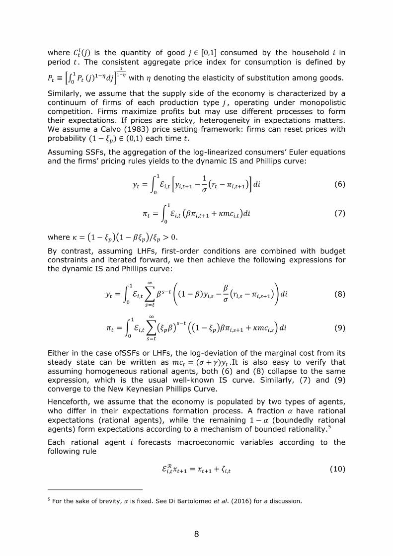
where 𝐶𝑡𝑖(𝑗) is the quantity of good 𝑗 ∈ [0,1] consumed by the household 𝑖 in
period 𝑡. The consistent aggregate price index for consumption is defined by
𝑃𝑡 ≡ [∫ 𝑃𝑡1
0(𝑗)1−𝜂𝑑𝑗]
1
1−𝜂 with 𝜂 denoting the elasticity of substitution among goods.
Similarly, we assume that the supply side of the economy is characterized by a
continuum of firms of each production type 𝑗 , operating under monopolistic
competition. Firms maximize profits but may use different processes to form
their expectations. If prices are sticky, heterogeneity in expectations matters. We assume a Calvo (1983) price setting framework: firms can reset prices with
probability (1 − 𝜉𝑝) ∈ (0,1) each time 𝑡.
Assuming SSFs, the aggregation of the log-linearized consumers’ Euler equations
and the firms’ pricing rules yields to the dynamic IS and Phillips curve:
𝑦𝑡 = ∫ ℰ𝑖,𝑡
1
0
[𝑦𝑖,𝑡+1 −1
𝜎(𝑟𝑡 − 𝜋𝑖,𝑡+1)] 𝑑𝑖 (6)
𝜋𝑡 = ∫ ℰ𝑖,𝑡
1
0
(𝛽𝜋𝑖,𝑡+1 + 𝜅𝑚𝑐𝑖,𝑡)𝑑𝑖 (7)
where 𝜅 = (1 − 𝜉𝑝)(1 − 𝛽𝜉𝑝)/𝜉𝑝 > 0.
By contrast, assuming LHFs, first-order conditions are combined with budget constraints and iterated forward, we then achieve the following expressions for
the dynamic IS and Phillips curve:
𝑦𝑡 = ∫ ℰ𝑖,𝑡
1
0
∑ 𝛽𝑠−𝑡
∞
𝑠=𝑡
((1 − 𝛽)𝑦𝑖,𝑠 −𝛽
𝜎(𝑟𝑖,𝑠 − 𝜋𝑖,𝑠+1)) 𝑑𝑖 (8)
𝜋𝑡 = ∫ ℰ𝑖,𝑡
1
0
∑(𝜉𝑝𝛽)𝑠−𝑡
∞
𝑠=𝑡
((1 − 𝜉𝑝)𝛽𝜋𝑖,𝑠+1 + 𝜅𝑚𝑐𝑖,𝑠) 𝑑𝑖 (9)
Either in the case ofSSFs or LHFs, the log-deviation of the marginal cost from its
steady state can be written as 𝑚𝑐𝑡 = (𝜎 + 𝛾)𝑦𝑡 .It is also easy to verify that
assuming homogeneous rational agents, both (6) and (8) collapse to the same expression, which is the usual well-known IS curve. Similarly, (7) and (9)
converge to the New Keynesian Phillips Curve.
Henceforth, we assume that the economy is populated by two types of agents,
who differ in their expectations formation process. A fraction 𝛼 have rational
expectations (rational agents), while the remaining 1 − 𝛼 (boundedly rational
agents) form expectations according to a mechanism of bounded rationality.5
Each rational agent 𝑖 forecasts macroeconomic variables according to the
following rule
ℰ𝑖,𝑡ℛ 𝑥𝑡+1 = 𝑥𝑡+1 + 𝜁𝑖,𝑡 (10)
5 For the sake of brevity, 𝛼 is fixed. See Di Bartolomeo et al. (2016) for a discussion.

9
where ℰ𝑖,𝑡ℛ is the expectation operator used by the rational agent 𝑖 to forecast
𝑥𝑡+1 at 𝑡 and 𝜁𝑖,𝑡 is an i.i.d. expectation error with zero mean defined in the
support identified by the agents considered (i.e., in the case of rational agents: (0, 𝛼)). Aggregation among rational agents then yields
∫ ℰ𝑖,𝑡ℛ
𝛼
0
𝑥𝑡+1𝑑𝑖 = 𝛼𝐸𝑡𝑥𝑡+1 (11)
The remaining 1 − 𝛼 agents have cognitive limitations and use heuristics to
forecast macro variables. As previously illustrated, the predicted aggregate dynamics depend on the assumption about horizon forecasts. SSFs form their expectations focusing on one-period ahead forecasts based on heuristics and
making mistakes in predicting the next period values for relevant aggregate macroeconomic variables. LHFs, instead, use heuristics to forecast
macroeconomic variables over an infinite horizon and make errors in those predictions.
Looking at the fraction 1 − 𝛼, we begin by assuming that agents are SSFs. They
set their behavior at time 𝑡 based on their expectations on consumption (output)
or price at price 𝑡 + 1. Households satisfy an Euler equation, while firms set their
price according to a Calvo’s pricing rule. However, differently from the traditional
case, SSFs’ expectations are based on some heuristics and affected by systematic errors. Boundedly rational agents form their beliefs based on a
simple perceived linear law of motion, i.e., 𝑥𝑡 = 𝑥𝑡−1. Therefore,
ℰ𝑖,𝑡ℬ 𝑥𝑡 = 𝑥𝑡−1 + 𝜁𝑖,𝑡 (12)
where ℰ𝑖,𝑡ℬ is the expectation operator used by boundedly rational agents.
Applying the law of iterated expectations, we obtain ℰ𝑡ℬ𝑥𝑡+1 = 𝑥𝑡−1 + 𝜁𝑖,𝑡 + 𝜁𝑖,𝑡+1,
then aggregating
∫ ℰ𝑖,𝑡ℬ
1
𝛼
𝑥𝑡+1𝑑𝑖 = (1 − 𝛼)𝑥𝑡−1 (13)
By imposing some minimal restrictions to the heuristics used by the SSFs, Branch and McGough (2009) show that (12) implies a micro-founded
representation of the sticky price New Keynesian model very similar to the traditional case. The generalization of the New Keynesian sticky price model to heterogeneous expectations, in fact, implies that the conditional expected values
of the textbook model are replaced by a convex combination of expectations operators (rational (11) and heuristics (13)).
Formally, the aggregate IS demand curve and the Phillips Curve become:
𝑦𝑡 = 𝛼𝐸𝑡𝑦𝑡+1 + (1 − 𝛼)𝑦𝑡−1 −𝑟𝑡 − 𝛼𝐸𝑡𝜋𝑡+1 − (1 − 𝛼)𝜋𝑡−1
𝜎 (14)
𝜋𝑡 = 𝛽[𝛼𝐸𝑡𝜋𝑡+1 + (1 − 𝛼)𝜋𝑡−1] + 𝜅𝑚𝑐𝑡 (15)
Now, let us look at the case of LHFs, they use heuristics to forecast macroeconomic variables over an infinite horizon. The selection of heuristics
takes place at the beginning of period 𝑡, when they observe and compare past

10
performances. Each predictor 𝜃𝑖 ∈ Θ, ∀𝑖 ∈ [0,1], is evaluated according to the past
squared forecast error (performance measure). The distribution of beliefs then
evolves over time as a function of past performances according to the continuous choice model (Diks and van der Weide, 2005). The distribution of
beliefs is normal, and its evolution is characterized by a mean equal to 𝑥𝑡−1 and
a finite variance that is decreasing in the agents’ sensitivity to differences in performances.
Aggregating among boundedly rational agents, we obtain
∫ ℰ𝑖,𝑡
1
𝛼
𝑥𝑡+1𝑑𝑖 = (1 − 𝛼) ∫ 𝜃𝑖Θ
𝑑𝑖 = (1 − 𝛼)𝜃𝑥𝑡−1 (16)
By using (16) into (8) and (9), we get the representation of the IS curve and
Phillips cure, which are respectively
𝑦𝑡 = 𝛼𝐸𝑡 ∑ 𝛽𝑠−𝑡
∞
𝑠=𝑡
[(1 − 𝛽)𝑦𝑠 −𝛽
𝜎(𝑟𝑠 − 𝜋𝑠+1)] +
+(1 − 𝛼) [𝑦𝑡−1 −𝛽
𝜎
(1 − 𝛽)𝑟𝑡 + 𝜃𝛽𝑟𝑡−1 − 𝜃𝜋𝑡−1
1 − 𝛽] (17)
and
𝜋𝑡 = 𝛼𝐸𝑡 ∑(𝜉𝑝𝛽)𝑠−𝑡
∞
𝑠=𝑡
[(1 − 𝜉𝑝)𝛽𝜋𝑠+1 + 𝜅𝑚𝑐𝑠] +
+(1 − 𝛼) [𝜃𝑘
1 − 𝜉𝑝𝛽𝑚𝑐𝑡−1 +
𝜃(1 − 𝜉𝑝)𝛽
1 − 𝜉𝑝𝛽𝜋𝑡−1] (18)
In equation the above equations, we assumed that the current interest rate is
observed by boundedly rational agents, while current output and inflation are not.
Independently of the fraction and the kind of boundedly rational agents, to
perform welfare analysis under model uncertainty, we need a second-order approximation of the utility function (5). The instantaneous loss can be written
as follows:
𝐿𝑡 =1
2[(𝛾 +
1
𝜎) 𝑦𝑡
2 + (𝜂2𝛾)𝑣𝑎𝑟𝑖(𝑝𝑡(𝑖)) +1
𝜎𝑣𝑎𝑟𝑖(𝑐𝑡(𝑖))] (19)
Due to the agents’ heterogeneity, the welfare criterion (19) is made up of three components. Beyond the traditional costs related to consumption variability and
price dispersion, there is an additional cost which captures the inequality in the
consumption of the different types of agents 𝑣𝑎𝑟𝑖(𝑐𝑡(𝑖)). Everything equal, the
cost reaches the maximum in case population is split in half which happens when
𝛼 = 0.5 . The cross-sectional variability of expectations, which involves
differences in consumption and labour/leisure choices, implies higher inequality.
11
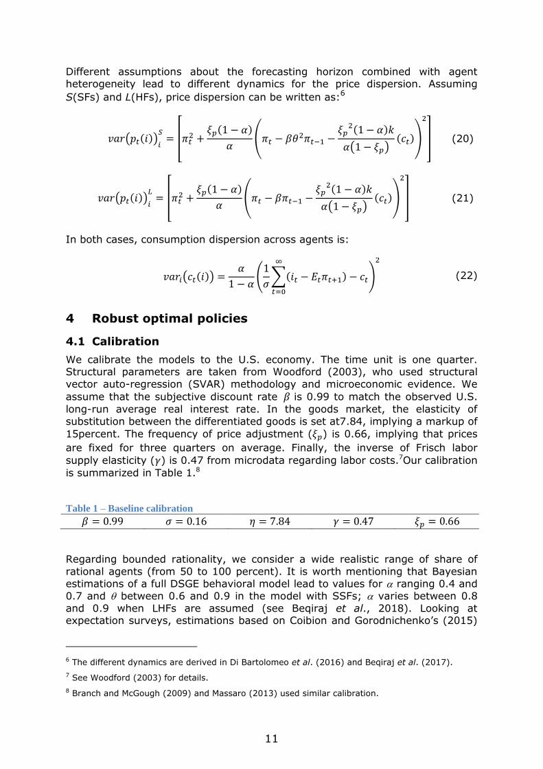
Different assumptions about the forecasting horizon combined with agent heterogeneity lead to different dynamics for the price dispersion. Assuming
S(SFs) and L(HFs), price dispersion can be written as:6
𝑣𝑎𝑟(𝑝𝑡(𝑖))𝑖
𝑆= [𝜋𝑡
2 +𝜉𝑝(1 − 𝛼)
𝛼(𝜋𝑡 − 𝛽𝜃2𝜋𝑡−1 −
𝜉𝑝2(1 − 𝛼)𝑘
𝛼(1 − 𝜉𝑝)(𝑐𝑡))
2
] (20)
𝑣𝑎𝑟(𝑝𝑡(𝑖))𝑖
𝐿= [𝜋𝑡
2 +𝜉𝑝(1 − 𝛼)
𝛼(𝜋𝑡 − 𝛽𝜋𝑡−1 −
𝜉𝑝2(1 − 𝛼)𝑘
𝛼(1 − 𝜉𝑝)(𝑐𝑡))
2
] (21)
In both cases, consumption dispersion across agents is:
𝑣𝑎𝑟𝑖(𝑐𝑡(𝑖)) =𝛼
1 − 𝛼(
1
𝜎∑(𝑖𝑡 − 𝐸𝑡𝜋𝑡+1)
∞
𝑡=0
− 𝑐𝑡)
2
(22)
4 Robust optimal policies
4.1 Calibration
We calibrate the models to the U.S. economy. The time unit is one quarter. Structural parameters are taken from Woodford (2003), who used structural
vector auto-regression (SVAR) methodology and microeconomic evidence. We
assume that the subjective discount rate 𝛽 is 0.99 to match the observed U.S.
long-run average real interest rate. In the goods market, the elasticity of
substitution between the differentiated goods is set at7.84, implying a markup of
15percent. The frequency of price adjustment (𝜉𝑝) is 0.66, implying that prices
are fixed for three quarters on average. Finally, the inverse of Frisch labor
supply elasticity (𝛾) is 0.47 from microdata regarding labor costs.7Our calibration
is summarized in Table 1.8
Table 1 – Baseline calibration
𝛽 = 0.99 𝜎 = 0.16 𝜂 = 7.84 𝛾 = 0.47 𝜉𝑝 = 0.66
Regarding bounded rationality, we consider a wide realistic range of share of
rational agents (from 50 to 100 percent). It is worth mentioning that Bayesian
estimations of a full DSGE behavioral model lead to values for ranging 0.4 and
0.7 and between 0.6 and 0.9 in the model with SSFs; varies between 0.8
and 0.9 when LHFs are assumed (see Beqiraj et al., 2018). Looking at expectation surveys, estimations based on Coibion and Gorodnichenko’s (2015)
6 The different dynamics are derived in Di Bartolomeo et al. (2016) and Beqiraj et al. (2017).
7 See Woodford (2003) for details.
8 Branch and McGough (2009) and Massaro (2013) used similar calibration.
12
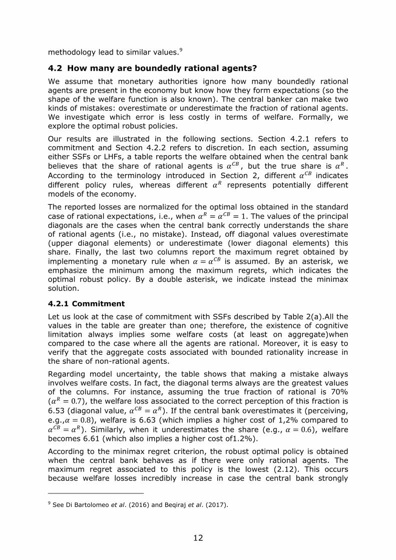
methodology lead to similar values.9
4.2 How many are boundedly rational agents?
We assume that monetary authorities ignore how many boundedly rational
agents are present in the economy but know how they form expectations (so the shape of the welfare function is also known). The central banker can make two kinds of mistakes: overestimate or underestimate the fraction of rational agents.
We investigate which error is less costly in terms of welfare. Formally, we explore the optimal robust policies.
Our results are illustrated in the following sections. Section 4.2.1 refers to commitment and Section 4.2.2 refers to discretion. In each section, assuming
either SSFs or LHFs, a table reports the welfare obtained when the central bank
believes that the share of rational agents is 𝛼𝐶𝐵 , but the true share is 𝛼𝑅 .
According to the terminology introduced in Section 2, different 𝛼𝐶𝐵 indicates
different policy rules, whereas different 𝛼𝑅 represents potentially different
models of the economy.
The reported losses are normalized for the optimal loss obtained in the standard
case of rational expectations, i.e., when 𝛼𝑅 = 𝛼𝐶𝐵 = 1. The values of the principal
diagonals are the cases when the central bank correctly understands the share of rational agents (i.e., no mistake). Instead, off diagonal values overestimate
(upper diagonal elements) or underestimate (lower diagonal elements) this share. Finally, the last two columns report the maximum regret obtained by
implementing a monetary rule when 𝛼 = 𝛼𝐶𝐵 is assumed. By an asterisk, we
emphasize the minimum among the maximum regrets, which indicates the optimal robust policy. By a double asterisk, we indicate instead the minimax
solution.
4.2.1 Commitment
Let us look at the case of commitment with SSFs described by Table 2(a).All the values in the table are greater than one; therefore, the existence of cognitive limitation always implies some welfare costs (at least on aggregate)when
compared to the case where all the agents are rational. Moreover, it is easy to verify that the aggregate costs associated with bounded rationality increase in
the share of non-rational agents.
Regarding model uncertainty, the table shows that making a mistake always
involves welfare costs. In fact, the diagonal terms always are the greatest values of the columns. For instance, assuming the true fraction of rational is 70%
(𝛼𝑅 = 0.7), the welfare loss associated to the correct perception of this fraction is
6.53 (diagonal value, 𝛼𝐶𝐵 = 𝛼𝑅). If the central bank overestimates it (perceiving,
e.g.,𝛼 = 0.8), welfare is 6.63 (which implies a higher cost of 1,2% compared to
𝛼𝐶𝐵 = 𝛼𝑅). Similarly, when it underestimates the share (e.g., 𝛼 = 0.6), welfare
becomes 6.61 (which also implies a higher cost of1.2%).
According to the minimax regret criterion, the robust optimal policy is obtained
when the central bank behaves as if there were only rational agents. The maximum regret associated to this policy is the lowest (2.12). This occurs
because welfare losses incredibly increase in case the central bank strongly
9 See Di Bartolomeo et al. (2016) and Beqiraj et al. (2017).

13
believes the economy is populated by non-rational agents, but there are instead only rational agents.10
Table 2(a) - Welfare losses under commitment with SSFs
Perceived True proportion (𝛼𝑅)
(𝛼𝐶𝐵) 0.5 0.6 0.7 0.8 0.9 1.0 Max
Min
Max
Regret
0.5 10.21 8.17 6.97 6.36 5.75 4.31 10.21** 3.31
0.6 10.34 8.08 6.61 5.71 5.09 3.88 10.34 2.88
0.7 10.61 8.19 6.53 5.40 4.67 3.63 10.61 2.63
0.8 11.01 8.45 6.63 5.32 4.41 3.49 11.01 2.49
0.9 11.57 8.91 6.95 5.46 4.32 3.42 11.57 2.42
1.0 12.33 9.68 7.69 6.11 4.74 1.00 12.33 2.12*
Assuming that agents are LHFs, commitment is described in Table 2(b). The
outcomes are like those described for SSFs’ case. The minimum among the maximum regret is obtained for the policy rule associated to the model where
𝛼𝐶𝐵 = 1.0. In this case, the maximum regret is 2.06.
Table 2(b) - Welfare losses under commitment with LHFs
Perceived True proportion (𝛼𝑅)
(𝛼𝐶𝐵) 0.5 0.6 0.7 0.8 0.9 1.0 Max
Min
Max
Regret
0.5 20.04 13.12 8.69 6.56 6.43 18.54 20.04** 17.54
0.6 20.11 13.05 8.41 5.89 5.08 9.64 20.11 8.64
0.7 20.30 13.10 8.34 5.65 4.40 5.57 20.30 4.57
0.8 20.59 13.23 8.37 5.59 4.07 3.78 20.59 2.78
0.9 20.77 13.31 8.48 5.68 3.98 3.08 20.77 2.08
1.0 21.83 15.11 9.75 6.08 4.04 1.00 21.83 2.06*
However, if the central bank takes its action based on the minimax criterion, the
scenario will change radically. In both cases, it in fact implies that the central bank should behave as the amount of boundedly rational agents in the economy is the highest irrespectively of its true share. The intuition is quite simple. As
long as the share of rational agents falls, the welfare loss increases.11 Then, when the share of boundedly rational agents is high, optimal policy requires
internalizing this information accounting exactly for them. As above explained, the two criteria can give misleading results.
10 Di Bartolomeo et al. (2016) focused upon a dichotomous scenario where the share of rational agents can only assume two given values (1 or 0.7). They found that, according to the minimax regret criterion, the optimal robust policy requires taking into account 30% of boundedly rational agents in both policy regimes.
11 Note that the highest loss for each policy correspond to those reported in columns (1), where
the share of rational agents is the lowest.

14
4.2.2 Discretion
Let us now investigate the effects of cognitive limitation when the central bank
operates in a discretionary fashion. Results are illustrated in Table 3(a) and 3(b), which refer to the cases of SSFs and LHFs.
Table 3(a) - Welfare losses under discretion with SSFs
Perceived True proportion (𝛼𝑅)
(𝛼𝐶𝐵) 0.5 0.6 0.7 0.8 0.9 1.0 Max
Min
Max
Regret
0.5 8.15 6.48 5.26 4.31 3.67 3.31 8.15** 2.31
0.6 8.19 6.49 5.27 4.33 3.63 3.24 8.19 2.24
0.7 8.31 6.53 5.28 4.35 3.63 3.19 8.31 2.19
0.8 8.52 6.64 5.32 4.37 3.64 3.17 8.52 2.17
0.9 8.85 6.88 5.46 4.41 3.65 3.15 8.85 2.15
1.0 9.32 7.32 5.84 4.68 3.73 1.00 9.32 1.17*
Table 3(b) - Welfare losses under discretion with LHFs
Perceived True proportion (𝛼𝑅)
(𝛼𝐶𝐵) 0.5 0.6 0.7 0.8 0.9 1.0 Max
Min
Max
Regret
0.5 16.79 11.69 8.14 7.68 29.70 344.26 16.79** 343.25
0.6 16.79 11.62 8.03 7.13 56.84 263.13 16.79 262.13
0.7 16.92 11.61 7.91 6.55 26.97 119.09 16.92 118.09
0.8 17.10 11.56 7.71 6.01 13.49 54.01 17.10 53.01
0.9 17.03 11.32 7.50 5.68 16.20 22.23 17.03 21.23
1.0 16.85 13.08 13.24 9.87 5.44 1.00 16.85 5.73*
Again, all values in the tables are greater than one, indicating welfare costs
compared to the case when all the agents are rational. The aggregate costs associated with bounded rationality increase in the share of non-rational agents.
Now, differently from the commitment regime, lowest losses implied by discretionary rules are no longer distributed along the main diagonal. Therefore, even if the central banker would be perfectly informed about the share of
rational agents (i.e., the true 𝛼𝑅 ), it would somehow find to ignore this
information, choosing a rule corresponding to 𝛼𝐶𝐵 < 𝛼𝑅 (it is easy to verify that
underestimation improves central bank’s performance).12
The rationale of the above result is as follows. In the textbook model, the discretionary planner may improve its policy efficacy by responding to inflation more aggressively than required by the society through a commitment to a
weight against inflation losses greater than that the society would commit to. We can refer to this case as optimal delegation.
The government appoints a central bank or delegates to the central bank an objective function that differs from the social welfare function derived
12 For example, if there are 90% of rational agents, it could be convenient for the central bank to ignore this information. Underestimating it, e.g., implementing the policy rule consistent with𝛼𝐶𝐵 =0.5, the loss is 3.67, which is lower than the loss obtained when the policy consistent with the true
model is chosen (3.63).

15
considering social beliefs and preferences. The delegation however improves the society (government’s) welfare measure. By committing to a more aggressive
behavior to inflation, if in the economy there is some inertia, the central bank can stabilize the expectation reducing the cost of stabilizing the current trade-off
between inflation and output (Clarida et al., 1999).
In our framework, inertia is intrinsic to boundedly rational agents’ behavior and discretionary rules associated to smaller share of rational agents might put more
pressure on inflation stabilization. Then the rationale is as above. An inefficient deviation from the welfare-consistent rule, due to the underestimation of
rational agents, leads to a more aggressive policy towards inflation. In turn, aggressiveness stabilizes rational agents’ expectations and improves the current trade-off between inflation variability and output gap.
Regarding robust optimal policies, as in the case of commitment, the maximum regret is always minimized implementing a policy which ignores that all agents
might be not rational. When agents are SSFs (cf. Table 3(a)), the optimal regret is 1.17, which is the lowest value of the last column of Table 3(a). Similarly, when they are LHFs (cf. Table 3(b)), the minimax regret value is 5.73. Both are
consistent with a policy that assumes =1.
As a result, based on Savage’s criterion, when the central bank knows how
expectations are formed but ignores the share of boundedly rational agents, robust policy design under discretion (and commitment) requires that the central banker should implement a policy consistent with the assumption that the
economy is as if all the agents are fully rational, ignoring the fraction of boundedly rational agents.
When the minimax criteria are considered, instead of minimizing the maximum regret, the picture is mixed and the optimal policy solution should consider highest bounded rationality in the economy. The minimax regret criterion takes
into account that certain realizations of the unknown state of nature (our correct model) are associated with relatively high losses regardless of the policy choice.
Whereas the minimax criterion has been criticized in the sense that it is not required to obey to the axiom of independence or irrelevant alternatives provided by Chernoff (1954), while decision making under it. The axiom, is
frequently used in the individual choice theory and states that if an alternative 𝑥
is chosen from a set 𝑇, and 𝑥 is also an element of a subset 𝑆 ∈ 𝑇 , then 𝑥 must
be chosen from 𝑆. That is, context in which alternatives are made should not
affect the selection of 𝑥 as the best option.13
4.3 Who is the boundedly rational agent?
In this section, we consider that the central bank knows the share of boundedly
rational agents (𝛼𝑅 = 𝛼𝐶𝐵) but ignores how expectations are formed. Specifically,
we assume that the central bank observes the correct economic structure
(constraints), but it can maximize the wrong welfare function. This occurs when the central banker misunderstands the kind of boundedly rational agents and adopts the wrong welfare criterion to design monetary policy.
13 Blume et al. (2006) assume that such an axiomatization of rationality can be interpreted in a restrictive sense meaning that agents have preferences which obey certain conditions only over
states under consideration and not over all possible states of the world, as supposed by Savage.

16
Results are illustrated in Tables 4(a) (commitment) and 4(b) (discretion). In each case, we have two possible models and two possible policies. We indicate
by "true" the true model and by "perceived" the model adopted by the central bank to select the welfare criterion. We consider model uncertainty for a large
range of observed shares of rational agents.14 For each share, robust policy is derived comparing welfare outcomes from a 4 by 4 matrix derived by considering the two possible models and the two possible policies (obtained by
using one of the two different welfare criteria). Regrets are reported in the last columns and the robust policy is indicated by an asterisk.
Let us discuss the results when the commitment regime is implemented (cf. Table 4(a)). Bold numbers are welfare losses obtained when there is no uncertainty, i.e., the monetary authority is able to minimize the welfare loss
consistent with the kind of boundedly rational agents. Welfare losses are decreasing in the share of rational agents in both frameworks (SSFs and LHFs).
Moreover, misunderstanding the true model always implies additional costs
(compare welfare outcomes by row).15
Regarding model uncertainty, as said, robust policies are derived by comparing regrets associated with the two different rules in the two alternative specifications of the economy. The robust policy is chosen by applying Savage’s
criterion. For any given share of rational agents, monetary policy should be designed assuming that agents always are SSFs.
Table 4(a) - Welfare losses with uncertainty about expectation formation process: commitment
Perceived Max Max
True 𝛼𝐿𝐻𝐹 𝛼𝑆𝑆𝐹 Min Regret
0.5 𝛼𝐿𝐻𝐹 20.04 22.71 29.34 19.13 𝛼𝑆𝑆𝐹 29.34 10.21 22.71** 2.67*
0.6 𝛼𝐿𝐻𝐹 13.05 15.97 23.25 15.17 𝛼𝑆𝑆𝐹 23.25 8.08 15.97** 2.92*
0.7 𝛼𝐿𝐻𝐹 8.34 10.88 18.03 11.50 𝛼𝑆𝑆𝐹 18.03 6.53 10.88** 2.54*
0.8 𝛼𝐿𝐻𝐹 5.59 7.61 13.42 8.10 𝛼𝑆𝑆𝐹 13.42 5.32 7.61** 2.02*
0.9 𝛼𝐿𝐻𝐹 3.98 5.71 9.27 4.95 𝛼𝑆𝑆𝐹 9.27 4.32 5.71** 1.73*
Table 4(b) replicates previous analysis in case the central bank acts under
discretion. The results reported are confirmed and the central bank robust policy requires assuming that all the agents are SSFs with the exception of the extreme case where the share of rational agents is 90%. The minimax criterion
leads to similar results in both policy regimes.
14 The full rationality 𝛼𝑅 = 1.0 is not illustrated because the two forecasts mechanisms collapse to
the standard rational expectations case and get same welfare losses.
15 For example, when the central bank knows that the share of boundedly rational agents is 20%, but the central banker wrongly believes that they are LHFs, the welfare loss is 13.42. By contrast,
if the central bank correctly understands that agents are SSFs, welfare loss decreases to 5.32.

17
Table 4(b) - Welfare losses with uncertainty about expectation formation process: discretion
Perceived Max Max
True 𝛼𝐿𝐻𝐹 𝛼𝑆𝑆𝐹 Min Regret
0.5 𝛼𝐿𝐻𝐹 13.11 17.80 20.91 14.76 𝛼𝑆𝑆𝐹 22.91 8.15 15.51** 4.69*
0.6 𝛼𝐿𝐻𝐹 8.99 13.80 17.47 11.80 𝛼𝑆𝑆𝐹 18.29 6.49 12.40** 4.81*
0.7 𝛼𝐿𝐻𝐹 6.03 10.43 14.15 9.03 𝛼𝑆𝑆𝐹 14.31 5.28 9.99** 4.40*
0.8 𝛼𝐿𝐻𝐹 4.34 8.21 10.91 6.38 𝛼𝑆𝑆𝐹 10.75 4.37 8.06** 3.87*
0.9 𝛼𝐿𝐻𝐹 3.86 7.79 7.74 3.87* 𝛼𝑆𝑆𝐹 7.52 3.65 6.39** 3.93
4.4 Bi-dimensional uncertainty
Central bankers might ignore both the share and how boundedly rational agents form their expectations. In this section, we intersect the previous two by
considering the cost of misunderstanding the shape of the welfare-based loss rule (ignoring if agents are SSFs or LHFs) and the cost of ignoring the share of
rational agents into the economy. In other words, uncertainty is bi-dimensional:
uncertainty about the share of rational agents () and uncertainty about the way
expectations are formed (SSF/LHF).
Combining the uncertainty about the share of rational agents (5 cases) and that regarding the way expectations are formed (2 cases), we obtain 10 possible
states of the world. The central banker observes the economic dynamics and implements monetary policy by choosing the welfare loss to minimize. As the
loss depends on both the share of rational agents and the way expectations are formed, ten policy options are also available (one for each perceived state of the world). Combining state of the worlds and perceived state of the world we can
represent all possible losses in a ten-by-ten table, and derive robust optimal policies. Again, we distinguish the case of commitment and discretion.
The losses obtained for each policy option in each possible state of the world are reported in Table 5(a). In the table is always assumed that the central bank can commit to a policy rule, minimizing the loss corresponding to the perceived
model constrained by the true model of the economy. Therefore, off diagonal terms represent misunderstanding of the economy by the central banker.
Looking at the table as a 4 blocks matrix (each block is a 10-by-10 matrix), the top-left and bottom-right blocks are clearly derived from Table 2(a) and 2(b)
from Section 4.2.1. In such a case, the central banker understands the way expectations are formed, but he can eventually over or under estimate the share of rational agents. The bottom-left and top-right blocks report the losses
obtained when the central banker also misunderstands the way expectations are formed: he believes that agents are SSF when they are LHFs and vice versa. It
reports the costs of double errors.
Central bankers’ misunderstandings are costlier when model uncertainty is related to two dimensions. For instance, assume that agents are SSFs and the
share of rational is 60%, if the central bank wrongly supposes that they are 50% but understands how expectations are formed, the loss is 8.2. But if the central
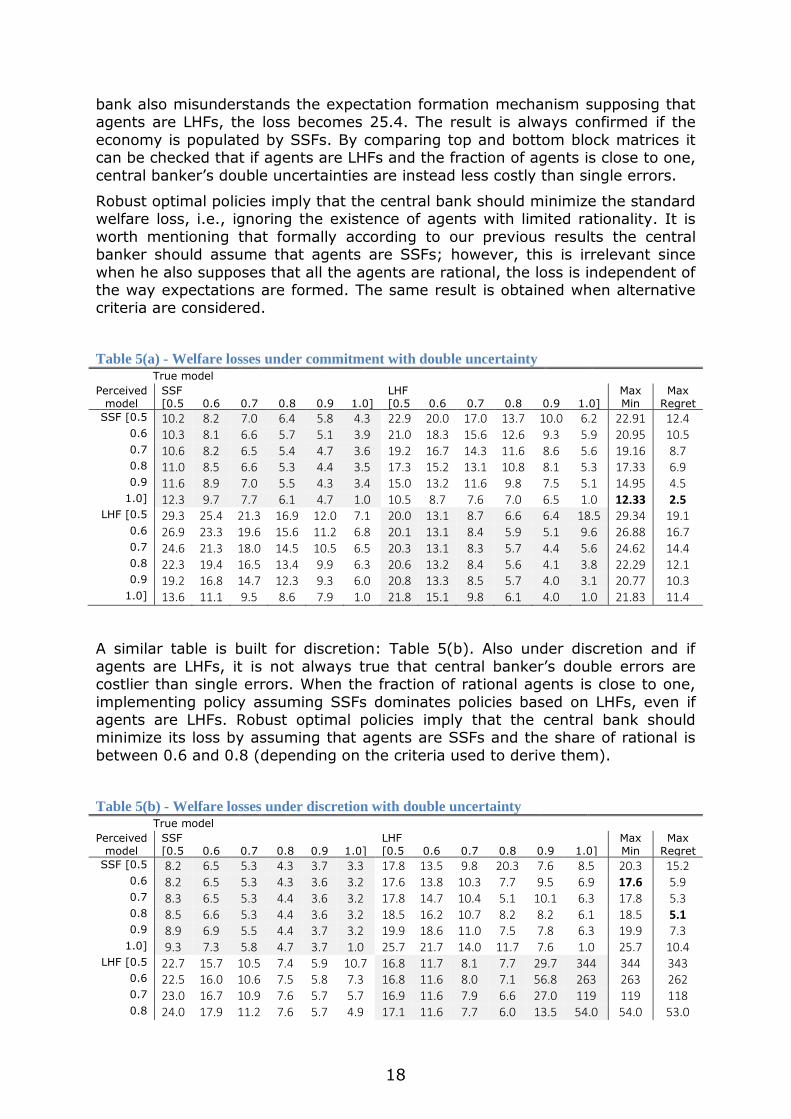
18
bank also misunderstands the expectation formation mechanism supposing that agents are LHFs, the loss becomes 25.4. The result is always confirmed if the
economy is populated by SSFs. By comparing top and bottom block matrices it can be checked that if agents are LHFs and the fraction of agents is close to one,
central banker’s double uncertainties are instead less costly than single errors.
Robust optimal policies imply that the central bank should minimize the standard welfare loss, i.e., ignoring the existence of agents with limited rationality. It is
worth mentioning that formally according to our previous results the central banker should assume that agents are SSFs; however, this is irrelevant since
when he also supposes that all the agents are rational, the loss is independent of the way expectations are formed. The same result is obtained when alternative criteria are considered.
Table 5(a) - Welfare losses under commitment with double uncertainty True model
Perceived model
SSF [0.5
0.6
0.7
0.8
0.9
1.0]
LHF [0.5
0.6
0.7
0.8
0.9
1.0]
Max Min
Max Regret
SSF [0.5 10.2 8.2 7.0 6.4 5.8 4.3 22.9 20.0 17.0 13.7 10.0 6.2 22.91 12.4 0.6 10.3 8.1 6.6 5.7 5.1 3.9 21.0 18.3 15.6 12.6 9.3 5.9 20.95 10.5 0.7 10.6 8.2 6.5 5.4 4.7 3.6 19.2 16.7 14.3 11.6 8.6 5.6 19.16 8.7 0.8 11.0 8.5 6.6 5.3 4.4 3.5 17.3 15.2 13.1 10.8 8.1 5.3 17.33 6.9 0.9 11.6 8.9 7.0 5.5 4.3 3.4 15.0 13.2 11.6 9.8 7.5 5.1 14.95 4.5
1.0] 12.3 9.7 7.7 6.1 4.7 1.0 10.5 8.7 7.6 7.0 6.5 1.0 12.33 2.5 LHF [0.5 29.3 25.4 21.3 16.9 12.0 7.1 20.0 13.1 8.7 6.6 6.4 18.5 29.34 19.1
0.6 26.9 23.3 19.6 15.6 11.2 6.8 20.1 13.1 8.4 5.9 5.1 9.6 26.88 16.7 0.7 24.6 21.3 18.0 14.5 10.5 6.5 20.3 13.1 8.3 5.7 4.4 5.6 24.62 14.4 0.8 22.3 19.4 16.5 13.4 9.9 6.3 20.6 13.2 8.4 5.6 4.1 3.8 22.29 12.1 0.9 19.2 16.8 14.7 12.3 9.3 6.0 20.8 13.3 8.5 5.7 4.0 3.1 20.77 10.3
1.0] 13.6 11.1 9.5 8.6 7.9 1.0 21.8 15.1 9.8 6.1 4.0 1.0 21.83 11.4
A similar table is built for discretion: Table 5(b). Also under discretion and if
agents are LHFs, it is not always true that central banker’s double errors are costlier than single errors. When the fraction of rational agents is close to one,
implementing policy assuming SSFs dominates policies based on LHFs, even if agents are LHFs. Robust optimal policies imply that the central bank should minimize its loss by assuming that agents are SSFs and the share of rational is
between 0.6 and 0.8 (depending on the criteria used to derive them).
Table 5(b) - Welfare losses under discretion with double uncertainty True model
Perceived model
SSF [0.5
0.6
0.7
0.8
0.9
1.0]
LHF [0.5
0.6
0.7
0.8
0.9
1.0]
Max Min
Max Regret
SSF [0.5 8.2 6.5 5.3 4.3 3.7 3.3 17.8 13.5 9.8 20.3 7.6 8.5 20.3 15.2 0.6 8.2 6.5 5.3 4.3 3.6 3.2 17.6 13.8 10.3 7.7 9.5 6.9 17.6 5.9 0.7 8.3 6.5 5.3 4.4 3.6 3.2 17.8 14.7 10.4 5.1 10.1 6.3 17.8 5.3 0.8 8.5 6.6 5.3 4.4 3.6 3.2 18.5 16.2 10.7 8.2 8.2 6.1 18.5 5.1 0.9 8.9 6.9 5.5 4.4 3.7 3.2 19.9 18.6 11.0 7.5 7.8 6.3 19.9 7.3
1.0] 9.3 7.3 5.8 4.7 3.7 1.0 25.7 21.7 14.0 11.7 7.6 1.0 25.7 10.4 LHF [0.5 22.7 15.7 10.5 7.4 5.9 10.7 16.8 11.7 8.1 7.7 29.7 344 344 343
0.6 22.5 16.0 10.6 7.5 5.8 7.3 16.8 11.6 8.0 7.1 56.8 263 263 262 0.7 23.0 16.7 10.9 7.6 5.7 5.7 16.9 11.6 7.9 6.6 27.0 119 119 118 0.8 24.0 17.9 11.2 7.6 5.7 4.9 17.1 11.6 7.7 6.0 13.5 54.0 54.0 53.0

19
0.9 26.3 20.2 11.5 7.7 5.7 4.6 17.0 11.3 7.5 5.7 16.2 22.2 26.3 21.2 1.0] 33.8 27.7 11.8 7.7 5.7 1.0 16.9 13.1 13.2 9.9 5.4 1.0 33.8 25.7
5 Conclusion
This paper investigated monetary policy optimal design under model uncertainty. It used non-Bayesian robust control techniques. We considered a sticky price DSGE economy and assumed that some agents behave according to some
limited rationality when they have to form their expectations about the future. Moreover, we also assumed that agents can be either short-sighted (SSFs) or
long-horizon forecasters (LHFs). The former behave according to their Euler equations, so, period-by-period, they need to forecast future one period ahead.
Instead, the latter behave according to their inter-temporal constraints, so they have to forecast the long-run expected values (e.g., their expected permanent income for the consumers). 16 The central bank then might face model
uncertainty ignoring the share of boundedly rational agents and/or how their expectations are formed (i.e., agents are SSFs or LHFs).
We began by focusing upon uncertainty about the true distribution of agents. The central bank knows how expectations are formed (and then the shape of the welfare loss) but ignores the share of rational agents populating the economy.
Second, we investigate robust policies when the central banker knows the fraction of boundedly rational agents but ignores whether the economy is
populated by SSFs or LHFs. Finally, the two previous forms of model uncertainty are simultaneously considered. We introduced a bi-dimensional model uncertainty, assuming that the central banker ignores both the share and the
forecasting mechanism of boundedly rational agents. In all the cases, we calculated robust policies for a wide range of the share of rational agents in the
economy, varying from 50 to 100 percent. Both commitment and discretion were considered.
Our results can be summarized as follows.
When model uncertainty only belongs to the true fraction of boundedly rational agents, minimax and minimax regret criterion lead to opposite policy
implications. The latter is associated to robust policies designed by ignoring the existence of boundedly rational agents in the economy. According to the former, instead, the robust policy requires considering the highest degree of bounded
rationality. The result holds for both commitment and discretion.
When model uncertainty only belongs to the mechanism boundedly rational
agents use to form their expectations, the central bank knows the share of rational agents but two kinds of mistakes can be made: assuming LHFs in a world where all the agents are SSFs or neglecting them in a context where
agents truly are long-sighted. We find that the policymaker should always conduct monetary policy by assuming that agents are SSFs. The result is
confirmed by using both non-Bayesian robust control techniques.
Combining the above cases, we also explore the case where bi-dimensional model uncertainty is introduced: a central banker who ignores both the share of
boundedly rational agents and their forecasts horizon. Additional welfare losses
16 If all the agents are rational, the assumption about the forecasting horizon does not matter.

20
due to double model uncertainty decrease as the number of rational forecasters increases in the economy. Our analysis suggested that the ability of the central
bank to recognize only the forecasts mechanism of non-rational agents, while still misunderstanding their share, would not always minimize welfare losses. If
the economy is populated by LHFs, it is not always true that central banker’s double errors are costlier than single errors. However, double uncertainty confirms the robust policy obtained in the case of commitment. By contrast,
under discretion, robust optimal policies are implemented considering that the share of rational agents is between 60% and 80%.
21
References
Adam, K. (2007), “Optimal monetary policy with imperfect common knowledge,” Journal of Monetary Economics, 54(2): 267–301.
Andolfatto, D., Hendry, S., and K. Moran, (2008), “Are inflation expectations
rational?”Journal of Monetary Economics, 55(2): 406–422.
Andrade, P. and H. Le Bihan (2013), “Inattentive professional forecasters,”
Journal of Monetary Economics, 60(8): 967–982.
Assenza, T., P. Heemeijer, C. Hommes and D. Massaro (2011), “Individual expectations and aggregate macro behavior,” CeNDEF Working Paper, 2011-1
University of Amsterdam.
Beqiraj, E., G. Di Bartolomeo, and C. Serpieri (2017), “Rational vs. long-run
forecasters: Optimal monetary policy and the role of inequality,” Macroeconomic Dynamics, forthcoming.
Beqiraj, E., G. Di Bartolomeo, M. Di Pietro, and C. Serpieri (2018), “Bounded-rationality and heterogeneous agents: Long or short forecasters?,” JRC Technical Report.
Blanchard, O. J. and C. M. Kahn (1980), “The solution of linear difference models under rational expectations,” Econometrica, 48(5): 1305–1311.
Blume, L., D. Easley, and J. Halperin (2006), “Redoing the foundations of decisiontheory, ” Mimeo, Cornell University.
Branch, W. A. (2004), “The theory of rationally heterogeneous expectations:
Evidence from survey data on inflation expectations,” The Economic Journal, 114(497): 592–621.
Branch, W.A. and B. McGough (2009), “A New Keynesian model with heterogeneous expectations,” Journal of Economic Dynamics and Control, 33(5): 1036–1051.
Branch, W. A. and B. McGough (2016), “Heterogeneous expectations and micro-foundations in macroeconomics,” forthcoming in Handbook of Computational
Economics, K. Schmedders and K.L. Judd (eds.), Elsevier Science, North-Holland, Vol. 4.
Brock, W. A. and C. H. Hommes (1997), “A rational route to randomness,”
Econometrica, 65(5): 1059-1096.
Brock, W. A. and C. H. Hommes (1998), “Heterogeneous beliefs and routes to
chaos in a simple asset pricing model,” Journal of Economic Dynamics and Control, 22(8-9): 1235-1274.
Brock, W. A. and S. N. Durlauf (2005), “Local robustness analysis: Theory and
application,” Journal of Economic Dynamics and Control, 29(11): 2067-2092.
Brock, W. A., S. N. Durlauf, and K. D. West (2003), "Policy evaluation in
uncertain economic environments," Brookings Papers on Economic Activity, 34(1): 235-322.
Brock, W. A., S. N. Durlauf, and K. D. West (2007), "Model uncertainty and
policy evaluation: Some theory and empirics," Journal of Econometrics, 136(2): 629-664.
22
Brzoza-Brzezina, M., M. Kolasa, G. Koloch, K. Makarski and M. Rubaszek (2013), “Monetary policy in a non-representative agents economy: a survey,” Journal of
Economic Surveys, 27(4): 641-669.
Calvo, G. A. (1983), “Staggered prices in a utility–maximizing framework,”
Journal of Monetary Economics, 12(3): 383–398.
Carroll, C. (2003), “Macroeconomic expectations of households and professional forecasters,” Quarterly Journal of Economics, 118(1): 269–298.
Cirillo, P., D. Delli Gatti, S. Desiderio, E.Gaffeo, M. Gallegati (2011), “Macroeconomics from the bottom-up,” Milan: Springer.
Chernoff, H. (1954), “Rational selection of decision functions,” Econometrica, 22: 422-443.
Clarida, R., J. Galí, and M. Gertler (2000), “Monetary policy rules and
macroeconomic stability: Evidence and some theory,” Quarterly Journal of Economics, 115(1): 147–180.
Coibion, O. and Y. Gorodnichenko (2015), “Information rigidity and the expectations formation process: A simple framework and new facts,” American Economic Review, 105(8): 2644–2678.
Deak, S., P. Levine, J. Pearlman, and B. Yang (2017), “Internal rationality, learning and imperfect information,” School of Economics, University of Surrey,
mimeo.
Del Negro, M., and S. Eusepi (2011), “Fitting observed inflation expectations,”
Journal of Economic Dynamics and Control, 35: 2105–2131.
Di Bartolomeo, G., M. Di Pietro, and B. Giannini (2016), “Optimal monetary policy in a New Keynesian model with heterogeneous expectations,” Journal of
Economic Dynamics and Control, 73: 373–387.
Di Bartolomeo, G., E. Beqiraj, and M. Di Pietro (2017), “Beliefs formation and
the puzzle of forward guidance power,” EconStor Preprints 175198, ZBW - German National Library of Economics.
Diks, C. and R. Van Der Weide (2005), “Herding, a-synchronous updating and
heterogeneity in memory in a CBS,” Journal of Economic Dynamics and Control, 29(4): 741–763.
Dovern, J. (2015), “A multivariate analysis of forecast disagreement: Confronting models of disagreement with survey data,” European Economic Review, 80: 16–35.
Dräger, L., M. J. Laml, D. Pfajfar (2016), “Are survey expectations theory-consistent? The role of central bank communication and news,” European
Economic Review, 85: 84–111.
Eusepi, S. and B. Preston (2011), “Expectations, learning, and business cycle fluctuations,” American Economic Review, 101(6): 2844–2872.
Evans, G. W. and S. Honkapohja (2001), “Learning and expectations in macroeconomics,” Princeton University Press.
Evans, G. W. and S. Honkapohja (2003), “Adaptive learning and monetary policy design,” Proceedings, Federal Reserve Bank of Cleveland: 1045-1084.
23
Evans, G. W. and G. Ramey (1992), “Expectation calculation and macroeconomic dynamics,” American Economic Review, 82(1): 207-224.
Evans, G. W. and G. Ramey (1998), “Claculation, adaptation and rational expectations,” Macroeconomic Dynamics, 2: 156-182.
Gaffeo, E., I. Petrella, D. Pfajfar and E. Santoro (2014), “Loss aversion and the asymmetric transmission of monetary policy,” Journal of Monetary Economics, 68:19-36.
Galì, J. and M. Gertler (1999), “Inflation dynamics: a structural econometric analysis,” Journal of Monetary Economics, 44: 195-222.
Galì, J., J. D. López-Salido, and J. Vallés (2004), “Rule of thumb consumers and the design of interest rate rules,” Journal of Money, Credit and Banking, 36(4): 739-763.
Gasteiger, E. (2014), “Heterogeneous expectations, optimal monetary policy, and the merit of policy inertia,” Journal of Monetary, Credit and Banking, 46(7):
1533–1554.
Gasteiger, E. (2017), “Optimal constrained interest-rate rules under heterogeneous expectations,” mimeo.
Hansen, L. and T. Sargent (2003), “Robust control of forward-looking models, Journal of Monetary Economics, 50: 581-604.
Hommes, C., J. Sonnemans, J. Tuinstra, and H. van de Velden (2005), “Coordination of expectations in asset pricing experiments,” Review of Financial
Studies, 18(3): 955–980.
Hommes, C. (2011), “The heterogeneous expectations hypothesis: Some evidence from the lab,” Journal of Economic Dynamics and Control, 35(1): 1–24.
Honkapohja, S., K. Mitra, and G. W. Evans (2013), “Notes on agents’ behavioral rules under adaptive learning and studies of monetary policy,” in
Macroeconomics at the Service of Public Policy, Chapter 4, Sargent, T. J. and J. Vilmunen (eds.), Oxford University Press, Oxford.
Kuester, K. and V. Wieland (2010), "Insurance Policies for Monetary Policy in the
Euro Area", MIT Press, vol. 8(4): 872-912.
Kurz, M., H. Jin, and M. Motolese (2005), “The role of expectations in economic
fluctuations and the efficacy of monetary policy,” Journal of Economic Dynamics and Control, 29(11): 2017-2065.
Levin, A. and J. Williams (2003), “Robust monetary policy with competing
reference model,” Journal of Monetary Economics, 50(5): 945-975.
Mankiw, N.G., R. Reis, and J. Wolfers (2004), “Disagreement about inflation
expectations,” in NBER Macroeconomics Annual 2003, M. Gertler and K. Rogoff (eds.), MIT Press, Cambridge, Vol. 18: 209–270.
Massaro, D. (2013), “Heterogeneous expectations in monetary DSGE models,”
Journal of Economic Dynamics and Control, 37(3): 680–692.
Milani, F. (2007). “Expectations, learning and macroeconomic persistence,”
Journal of Monetary Economics, 54(7): 2065–2082.
Milani, F. (2011). “Expectation shocks and learning as drivers of the business cycle,” Economic Journal, 121(552): 379–401.

24
Pfajfar, D. and E. Santoro (2010), “Heterogeneity, learning and information stickiness in inflation expectations,” Journal of Economic Behavior and
Organization, 75(3): 426–444.
Preston, B. (2006), “Adaptive learning, forecast-based instrument rules and
monetary policy,” Journal of Monetary Economics, 53(3): 507–535.
Roberts, J. M. (1997), “Is inflation sticky?,” Journal of Monetary Economics, 39(2): 173-196.
Savage, L. (1951), “The theory of statistical decision,” Journal of the American Statistical Association, 46(253): 55-67.
Sims, C. A. (2003), “Implications of rational inattention,” Journal of Monetary Economics, 50(3): 665–690.
Wald, A. (1950), “Statistical decision functions,” New York: John Wiley.
Walsh, C. E. (2010), “Monetary theory and policy,” The MIT Press, Cambridge Massachusetts.
Woodford, M. (1999), “Optimal monetary policy inertia,” The Manchester School, 67(Suppl.): 1–35.

25
List of tables
Table 1- Baseline calibration
Table 2(a) - Welfare losses under commitment with SSFs
Table 2(b) - Welfare losses under commitment with LHFs
Table 3(a) - Welfare losses under discretion with SSFs
Table 3(b) - Welfare losses under discretion with LHFs
Table 4(a) - Welfare losses with uncertainty about expectation formation
process: commitment
Table 4(b) - Welfare losses with uncertainty about expectation formation
process: discretion
Table 5(a) - Welfare losses under commitment with double uncertainty
Table 5(b) - Welfare losses under discretion with double uncertainty

GETTING IN TOUCH WITH THE EU
In person
All over the European Union there are hundreds of Europe Direct information centres. You can find the address of the centre nearest you at: http://europea.eu/contact
On the phone or by email
Europe Direct is a service that answers your questions about the European Union. You can contact this service:
- byfreephone: 00 800 6 7 8 9 10 11 (certain operators may charge for these calls),
- at the following standard number: +32 22999696, or
- by electronic mail via: http://europa.eu/contact
FINDING INFORMATION ABOUT THE EU
Online
Information about the European Union in all the official languages of the EU is available on the Europa website at: http://europa.eu
EU publications You can download or order free and priced EU publications from EU Bookshop at:
http://bookshop.europa.eu. Multiple copies of free publications may be obtained by contacting Europe
Direct or your local information centre (see http://europa.eu/contact).

XX-N
A-x
xxxx-E
N-N
doi:10.2760/66451
ISBN 978-92-79-82752-5
KJ-N
A-2
9210-E
N-N