Robust Look-ahead Three-phase Balancing of Uncertain Distribution Loads

Xinbo GengDepartment of Electrical and

Computer EngineeringTexas A&M University

College Station, TXxbgeng@tamu.edu

Swati GuptaSchool of Industrial and

Systems EngineeringGeorgia Institute of Technology

Atlanta, GAswatig@gatech.edu

Le XieDepartment of Electrical and

Computer EngineeringTexas A&M University

College Station, TXle.xie@tamu.edu

Abstract

Increasing penetration of highly variablecomponents such as solar generation and electricvehicle charging loads pose significant challengesto keeping three-phase loads balanced in moderndistribution systems. Failure to maintain balance acrossthree phases would lead to asset deterioration andincreasing delivery losses. Motivated by the real-worldneeds to automate and optimize the three-phasebalancing decision making, this paper introduces arobust look-ahead optimization framework that pursuesbalanced phases in the presence of demand-sideuncertainties. We show that look-ahead moving windowoptimization can reduce imbalances among phasesat the cost of a limited number of phase swappingoperations. Case studies quantify the improvementsof the proposed methods compared with conventionaldeterministic phase balancing. Discussions on possiblebenefits of the proposed methods and extensions arepresented.

1. Introduction

Increasing levels of distributed energy resources,together with more active participation of demand sideprograms, have introduced higher levels of uncertaintiesto distribution grid operations. One fundamental taskfor distribution system operators (DSOs) is to keep threephases as balanced as possible over a long period oftime. However, the increasing variability coming fromend users requires DSOs to revisit this old problemwith modern techniques. Imbalanced three phases couldlead to higher risks of equipment failures [1], increaseddelivery losses [2], potential relay malfunctioning [3],additional asset reinforcement costs [4], and issuesrelated with voltage imbalances [5–8]. In particular,there is increasing need to develop solutions that cankeep three phases balanced in the presence of highuncertainties from end users over a period of time (e.g.over the course of a day). In this paper, we provide a

novel and scalable solution for addressing this problem.From a DSO’s perspective, there are three levels

of decisions that can be made to ensure reliable andefficient delivery of electricity to end-users duringnormal conditions. At the highest level, it canengage with transmission-level voltage/reactive poweroptimization routine to regulate its voltage level at thepoint of interconnection with the backbone grid [9, 10].At the medium level, modern distribution operator couldcontrol various sectionalizers and tie switches in orderto optimize the topology of a distribution system [11,12]. At the lowest level, DSOs need to optimize theassignment of each load (or each cluster of loads) toappropriate phases in order to keep the three phasebalanced during a wide range of operating conditions.This paper addresses the issue at the lowest level.

There is a large body of literature that addresses theissue of keeping three phases balanced in distributionsystems. The phase balancing problem has beentraditionally formulated as a mixed integer linearprogram (MILP) [1]. Due to the computationalintractability of mixed integer programs, manyoptimization techniques and heuristics have beenapplied to phase balancing: simulated annealing [13],expert systems [14], particle swarm optimization [15],immune algorithm [3, 16] and dynamic programming[17]. These works [1,3,14–17] typically consider eithera single snapshot or use average loads over a long periodof time. In [18,19], the authors demonstrate the benefitsof extending the phase balancing problem to multiplesnapshots and utilizing daily load patterns. It is worthmentioning that [1, 3, 14–19] solve the deterministicphase balancing problem. Uncertainties as well asinter-temporal variabilities have not been taken intoaccount in the problem of phase balancing. This is thekey gap we attempt to bridge in this work.

The reminder of this paper is organized as follows:Section 2 introduces robust optimization; Section 3first reviews the deterministic phase balancing problem,which is enhanced to a robust optimization problemin Section 3.3. The proposed robust look-ahead phase

Proceedings of the 52nd Hawaii International Conference on System Sciences | 2019

URI: https://hdl.handle.net/10125/59790ISBN: 978-0-9981331-2-6(CC BY-NC-ND 4.0)

Page 3542

balancing problem is in Section 3.4. Case studiesand discussions are presented in Section 4 and 5.Conclusions and future works are in Section 6.

2. Robust Optimization: Preliminaries

Broadly speaking, there are two approaches fordecision making in uncertain environments: stochasticoptimization (SO) and robust optimization (RO).SO relies on probabilistic models to explain theuncertainties in data and often results in solutionsthat are sensitive to these assumptions1. On theother hand, RO incorporates a set-based deterministicmodel of the uncertainty such that the optimal solutionprotects against all realizations in the uncertainty set.Compared with SO, one significant advantage of ROis the computational tractability, which is importantfor the phase balancing problem to be applicablein real-world scenarios. Moreover, it has beenobserved that robust solutions are competitive with thedeterministic solutions in terms of cost, while beingmore robust to unplanned uncertainties in the data.Robust optimization also does not need to assume anyprobabilistic information about the uncertain quantities[21].

We consider the following row-uncertain robustlinear optimization problem, where the row vectors αiare uncertain in each constraint:

minimizex

γᵀx (1a)

subject to αᵀi x ≤ βi, ∀αi ∈ Ui, (1b)i = 1, 2, · · · ,m.

Formulation (1) seeks an optimal solution x ∈ Rn that isfeasible to m linear uncertain constraints αᵀ

i x ≤ βi, inwhich the uncertain vector of parameters αi can take anyvalues from the uncertainty set Ui. A common choice isthe polyhedral uncertainty set defined as

Ui := {αi : Hiαi ≤ hi}, i = 1, 2, · · · ,m, (2)

where Hi ∈ Rk×n and hi ∈ Rk depict k inequalitiesthat define a polyhedron. Such uncertainty sets havebeen successful in capturing insights from probabilitytheory to obtain more realistic models. For instance, ifthe data is generated independently from a probabilitydistribution then the well-known central limit theoremstates that the appropriately normalized average ofvariables tends to a normal distribution. The centrallimit theorem can be written as a polyhedral uncertaintyset that protects against all realizations of data that

1We refer an interested reader to [20] for a survey on stochasticmodeling and techniques.

satisfy the central limit theorem [22]. Its parameterscan be set such that if the data was generated via agiven probability distribution, then the uncertainty setcaptures provably 95% − 99% of possible scenarios.This provides a clean way to incorporate probabilisticinformation. We refer the reader to [23] for a moredetailed survey on robust optimization techniques.

In the definition of a polyhedral uncertainty set U ={α ∈ Rn|Hα ≤ h} where H ∈ Rk×n, the constraintαᵀx ≤ β ∀α ∈ U is equivalent to

b ≥ maximizeα

xᵀα (3a)

subject to Hα ≤ h. (3b)

Let p ∈ Rk+ be the dual variable for (3b). Then the duallinear program of (3) is:

minimizep

hᵀp (4a)

subject to Hᵀp = x, (4b)p ≥ 0. (4c)

By weak duality, any feasible solution p of (4) for agiven x provides a lower bound to (3), i.e. hᵀp ≤(∗)

maxα∈U αᵀx ≤ b, and the inequality (*) is tight for the

optimal solution of the dual formulation in (4), by strongduality.

Therefore the uncertain constraints αᵀi x ≤ βi ∀αi ∈

Ui are equivalent to the following deterministicconstraints:

hᵀi pi ≤ βi, Hᵀi pi = x, pi ≥ 0,

where each pi ∈ Rk+ is a vector of auxiliary variablescorresponding to the ith constraint in (1). The robustformulation (1) with polyhedral uncertainty sets Ui isthen equivalent to the following linear program [24]:

minimizex

γᵀx (5a)

subject to hᵀi pi ≤ βi, (5b)Hᵀi pi = x, (5c)

pi ∈ Rk+, i = 1, 2, · · ·m. (5d)

One major advantage of using a polyhedraluncertainty set is its computational tractability. Thereformulation of the robust linear program (1) asthe deterministic linear program (5) involves a fewmore variables and this does not increase the overallcomputational complexity [24].

Page 3543

3. Formulations of Phase BalancingProblems

3.1. Nomenclature

Time dependent variables are represented with ·[t],e.g. d[t] is the demand at time t. Matrices arerepresented using capital letters and uncertainty sets arein calligraphic font. | · | is the absolute value functionand ᵀ denotes transpose of matrices or vectors. By 1, wemean the vector of all ones in the appropriate dimension(typically n in this paper, e.g. in (6b) 1 ∈ Rn).

3.2. Deterministic Phase Balancing

We briefly review the conventional formulation ofphase balancing in this subsection. Formulation (6)presented below is a slight variation of the original onein [1].

minimizea,b,c,ua,ub,uc

max{ua, ub, uc} (6a)

subject to ua = |dᵀ(a− 1

3)|, (6b)

ub = |dᵀ(b−1

3)|, (6c)

uc = |dᵀ(c−1

3)|, (6d)

a+ b+ c = 1, (6e)a, b, c ∈ {0, 1}n, (6f)ua, ub, uc ∈ R+. (6g)

Phase balancing aims at finding the most balancedassignment of n loads d ∈ Rn to three phases (A,B,C).Phase balancing commonly relies on phase swapping(or re-phasing) actions to reduce imbalances. Phaseswapping typically happens at the feeder level, duringmaintenance or restoration periods [1]. Phase swappingactions are depicted by decision variables a, b and c,all of which are binary vectors with dimension equalto the number of loads, where ai = 1 (similarly,bi, ci = 1) denotes load di is assigned to phase A(similarly, to phase B, C), and 0 indicates di is notassigned to that phase. Constraint (6e) ensures thateach load must be assigned to exactly one phase2.Variables ua, ub, uc represent single-phase imbalances,namely the difference of load on phase A (B,C) fromthe uniformly balanced case dᵀ1/3. The objective (6a)is to minimize the largest imbalance amongst the threephases. The original formulation in [1] minimizes the

2For simplicity, we only consider single-phase loads in this paper.Extensions to multi-phase loads are in Section 5.3.

largest differences between any two phases, i.e.

minimizea,b,c∈{0,1}n

max{|dᵀ(b− a)|, |dᵀ(b− c)|, |dᵀ(a− c)|}.

(7)

These two formulations are closely related in thefollowing sense. Let the total loads assigned to phasesA, B and C be x, y and z respectively, and let thetotal overall load be x + y + z = dᵀ1. Without lossof generality, let x ≤ y ≤ z which implies x ≤dᵀ1/3 ≤ z. So, the objective value of (7) will bez − x whereas the objective value of (6) for such anassignment will be max{dᵀ1/3−x, z−dᵀ1/3}, but notethat z−x ≤ 2max{1/3−x, z−dᵀ1/3}. Therefore, theoptimal solution of (7) will be at most twice the optimalsolution of (6) (and similarly, optimal solution of (7) isat least the optimal solution of (6)). Further, we believethat our formulation in (6) meets the intuitive notion ofphase balancing better than (7). To see this, considera total given demand of 21 kW. Formulation (7) doesnot differentiate between the assignments 2,9,10 kW and3,7,11 kW on each phase. For either assignment, themaximum difference between the assigned loads is 8kW. However, our formulation (6) would prefer 3,7,11as a solution since it minimizes the maximum deviationfrom the average. The absolute value constraints (6b),(6c) and (6d) can be reformulated to obtain an equivalentmixed integer linear program [25]:

minimizea,b,c,u

u (8a)

subject to − u ≤ dᵀ(a− 1

3) ≤ u, (8b)

− u ≤ dᵀ(b− 1

3) ≤ u, (8c)

− u ≤ dᵀ(c− 1

3) ≤ u, (8d)

a+ b+ c = 1, (8e)a, b, c ∈ {0, 1}n, u ∈ R+. (8f)

3.3. Robust Phase Balancing

In deterministic phase balancing problem (6), loadvector d represents the average load level during a longperiod, without any uncertainties. Motivated by therapid growth of highly variable resources in distributionsystems, we connect conventional phase balancing withrobust optimization and formulate the following robust

Page 3544

phase balancing problem:

minimizeu,a,b,c

u (9a)

subject to − u ≤ dᵀ(a− 1

3) ≤ u,∀d ∈ D, (9b)

− u ≤ dᵀ(b− 1

3) ≤ u,∀d ∈ D, (9c)

− u ≤ dᵀ(c− 1

3) ≤ u,∀d ∈ D, (9d)

a+ b+ c = 1, (9e)a, b, c ∈ {0, 1}n, u ∈ R+. (9f)

The major difference between robust phase balancing(9) and the deterministic version (8) is that: insteadof seeking solutions (a, b, c) that are feasible for theaverage or expected load vector d, (9) seeks solutionsrobust to all realizations of d in an uncertainty set D.The uncertainty setD can be constructed using historicaldata or approximated with prior knowledge.

Similar to Section 2, formulation (9) with polyhedraluncertainty set D = {d : Hd ≤ h} can be rewritten asan MILP (10).

minimizep,q,a,b,c,u

u (10a)

subject to hᵀpa ≤ u, Hᵀpa = a− 1

3, (10b)

hᵀqa ≤ u, Hᵀqa =1

3− a, (10c)

hᵀpb ≤ u, Hᵀpb = b− 1

3, (10d)

hᵀqb ≤ u, Hᵀqb =1

3− b, (10e)

hᵀpc ≤ u, Hᵀpc = c− 1

3, (10f)

hᵀqc ≤ u, Hᵀqc =1

3− c, (10g)

a+ b+ c = 1, (10h)a, b, c ∈ {0, 1}n, u ∈ R+, (10i)

pa, pb, pc, qa, qb, qc ∈ Rk+. (10j)

where pa, pb, pc and qa, qb, qc are auxiliary variables.

3.4. Robust Look-ahead Phase Balancing

The problem formulated in Section 3.3 considersonly a single snapshot (e.g. one hour) decisionmaking for robust phase balancing. However,one key component of costs comes from frequent

phase swapping actions of loads. Therefore, it isimportant to consider the phase balancing problem in amulti-time-horizon setting. We formulate it as a robustlook-ahead phase balancing problem, much like theusual practices in [26, 27].

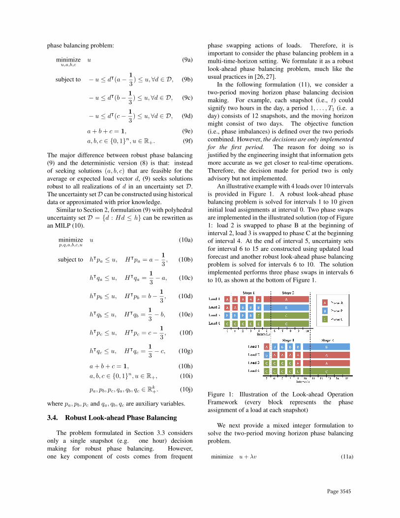
In the following formulation (11), we consider atwo-period moving horizon phase balancing decisionmaking. For example, each snapshot (i.e., t) couldsignify two hours in the day, a period 1, . . . , T1 (i.e. aday) consists of 12 snapshots, and the moving horizonmight consist of two days. The objective function(i.e., phase imbalances) is defined over the two periodscombined. However, the decisions are only implementedfor the first period. The reason for doing so isjustified by the engineering insight that information getsmore accurate as we get closer to real-time operations.Therefore, the decision made for period two is onlyadvisory but not implemented.

An illustrative example with 4 loads over 10 intervalsis provided in Figure 1. A robust look-ahead phasebalancing problem is solved for intervals 1 to 10 giveninitial load assignments at interval 0. Two phase swapsare implemented in the illustrated solution (top of Figure1: load 2 is swapped to phase B at the beginning ofinterval 2, load 3 is swapped to phase C at the beginningof interval 4. At the end of interval 5, uncertainty setsfor interval 6 to 15 are constructed using updated loadforecast and another robust look-ahead phase balancingproblem is solved for intervals 6 to 10. The solutionimplemented performs three phase swaps in intervals 6to 10, as shown at the bottom of Figure 1.

Figure 1: Illustration of the Look-ahead OperationFramework (every block represents the phaseassignment of a load at each snapshot)

We next provide a mixed integer formulation tosolve the two-period moving horizon phase balancingproblem.

minimize u+ λv (11a)

Page 3545

subject to − u ≤ (d[t])ᵀ(a[t]− 1

3) ≤ u, ∀d[t] ∈ Dt,

(11b)

− u ≤ (d[t])ᵀ(b[t]− 1

3) ≤ u, ∀d[t] ∈ Dt,

(11c)

− u ≤ (d[t])ᵀ(c[t]− 1

3) ≤ u, ∀d[t] ∈ Dt,

(11d)

t = 1, 2, · · · , T1

− v ≤ (d[t])ᵀ(a[T1]−1

3) ≤ v,∀d[t] ∈ Dt,

(11e)

− v ≤ (d[t])ᵀ(b[T1]−1

3) ≤ v,∀d[t] ∈ Dt,

(11f)

− v ≤ (d[t])ᵀ(c[T1]−1

3) ≤ v,∀d[t] ∈ Dt,

(11g)

t = T1 + 1, T1 + 2, · · · , T2

T1∑t=1

(1ᵀ|a[t]− a[t− 1]|+ 1ᵀ|b[t]− b[t− 1]|

+ 1ᵀ|c[t]− c[t− 1]|)≤ 2s,

(11h)

a[t] + b[t] + c[t] = 1, (11i)

a[t], b[t], c[t] ∈ {0, 1}n, u, v ∈ R+, (11j)t = 1, 2, · · · , T1.

In the above formulation (11), the first periodconsists of T1 snapshots (t = 1, 2, · · · , T1).It determines the phase swapping actions to beimplemented. Similar to previous formulations, ai[t] =1 indicates load di[t] is assigned to phase A at time t(t = 1, 2, · · · , T1). (11b)-(11d) are robust constraintsfor period 1. It is worth noting that each snapshot has itsown uncertainty set d[t] ∈ Dt. This allows (11) to takeadvantage of the temporal patterns of uncertain loads.As illustrated in Figure 1, no phase swapping actionsare considered for period 2. Formulation (11) seeksfixed load assignments with small phase imbalances forperiod 2. The decision variables of the second period area[T1], b[T1] and c[T1]. Constraints (11e)-(11g) relate todecisions in period 2.

We do not allow phase swapping actions in thesecond period of (11) for two important reasons: (a)uncertainties for the second period could be significantlylarger than in the first one, over-optimization withlarge uncertainties might lead to conservative solutions;(b) the problem size will be twice larger if weconsider phase swapping in both periods thus hurting

performance. Recall that phase balancing is an MILP,the computational burden could be prohibitive3

Variables u and v denote the largest single-phaseimbalance that occurs in the two periods, respectively.Choosing a proper value of parameter λ ∈ R+ couldachieve a balance between the optimality in short termand long term.

Given current industrial practice, swapping loadsfrom one phase to another typically requires manualoperations, which incurs extra costs on humanresources, maintenance expenses and planned outageduration [1]. Constraint (11h) limits the maximumnumber of phase swapping actions in the first period.Parameter s denotes the budget of swapping actions.Without constraint (11h), a large amount of phaseswapping actions could be recommended, which is notaffordable for utility companies [1].

For each snapshot t = 1, 2, · · · , T2, the polyhedraluncertainty set is defined as

Dt = {d[t] : Htd[t] ≤ ht} (12)

By introducing auxiliary variables, (11) is equivalentto an MILP (15).

It is worth mentioning that a recent paper [29]proposes a related but different approach with stochasticoptimization. It minimizes the expected loss functionover a time horizon with respect to uncertainties fromloads and electricity prices. While its decision variablesdenote the charging and discharging rates of energystorages, load assignments remain unchanged and nophase swapping actions are considered.

4. Case Study

4.1. Load Data

The load profiles are from dataset “R1-12.47-4” of[30]. It models a heavily populated suburban areacomposed mainly of single family homes and heavycommercial loads [31]. The dataset “R1-12.47-4” ispopulated with hourly averaged load data from a utilitycompany in the West Coast of the United States [30].The original dataset is publicly available on catalog.data.gov. The dataset contains 74 hourly loadprofiles of 365 days. We use the first 30 days and scalethem randomly to avoid identical load profiles.

Figure 2 visualizes the modified dataset.

3We actually tested the case in which phase swapping is consideredin both periods. Gurobi [28] took 12 hours to converge and the solutionwas comparable to the current formulation in (11).

Page 3546

(a) average daily load profiles with standard deviations (each colorrepresents one load)

(b) profiles of load 16 (different colors represent different days)

Figure 2: Modified Load Dataset “R1-1247-4”

4.2. Construct Uncertainty Set

In order to demonstrate the benefits ofrobustification, we use the following polyhedraluncertainty sets for the robust Phase Balancing (r-PB)and robust Look-ahead Phase Balancing (r-LAPB)problems:

D = {d ∈ Rn : d̂ ≤ d− d ≤ d̂} (13)

Dt = {d[t] ∈ Rn : (1− ρt)d[t] ≤ d[t] ≤ (1 + ρt)d[t]}(14)

where d ∈ Rn or d[t] ∈ Rn represent the average

load or forecast value, and d̂ ∈ Rn denotes the largestdeviation of load d. Problem r-PB (9) with d̂ = 0 isequivalent with deterministic Phase Balancing (d-PB)(6). Values of d, d[t] and d̂ are estimated from themodified “R1-1247-4” dataset. These uncertainty setscan be viewed as simple relaxations of the centrallimit theorem based sets (which can risk the solutionbeing too conservative), but they already show asignificant improvement in our experiments compared

Table 1: Parameters

n T1 T2 λ ρt (period1) ρt (period2)74 24 48 1/3 10% 30%

to deterministic solutions.For r-LAPB, the level of robustness ρt depends on

the forecast accuracy or confidence. Larger ρt indicateslower forecast accuracy. Definition of Dt in (13)-(14)assumes that the load forecast is unbiased and boundedby ρt. For r-LAPB, ρt in the first period (i.e. 24 hours)is set to be 10% (t = 1, 2, · · · , 24) and ρt = 30% forthe second period (t = 25, 26, · · · , 48).

For d-PB (6), load vector d is the average hourly loadof 30 days. There is no uncertainty associated.

4.3. Simulation Results

Simulations are performed on a desktop with Inteli7-2600 8-core CPU@3.40GHz and 16GB memory. Thephase balancing problems are solved using YALMIP[32, 33] and Gurobi [28]. The optimality gap of everysolution is smaller than 0.1%. Key results are presentedin Figure 3 and Table 2.

The performance of three formulations are evaluatedusing three metrics: between-phase kW differenceω, single-phase kW difference ν and single-phasepercentage difference υ, which are defined below:

ω := max{|dᵀ(a− b)|, |dᵀ(a− c)|, |dᵀ(b− c)|},

ν := max{|dᵀ(a− 1/3)|, |dᵀ(b− 1/3)|, |dᵀ(c− 1/3)|},

υ := max{|1− 3dᵀa

dᵀ1|, |1− 3dᵀb

dᵀ1|, |1− 3dᵀc

dᵀ1|}.

Compared with d-PB, robust phase balancing(r-PB) reduces both between-phase and single-phaseimbalances by around 11%, the standard deviationsof imbalances are reduced by more than 20%. Itis also worth mentioning that the time to solve r-PBis significantly reduced due to more restricted searchspace since the robust solutions must be feasible for alldemand realizations.

Table 2 shows that the imbalances could besignificantly reduced by incorporating look-aheadoperations. For example, r-LAPB with 3 swappingactions per day reduces both between-phase andsingle-phase kW differences by 30% on average.

Figure 3 and Table 2 also demonstrate the trade-offbetween performance and computation complexity. Ingeneral, more frequent phase swapping operations leadto less imbalances among phases, while the time of

Page 3547

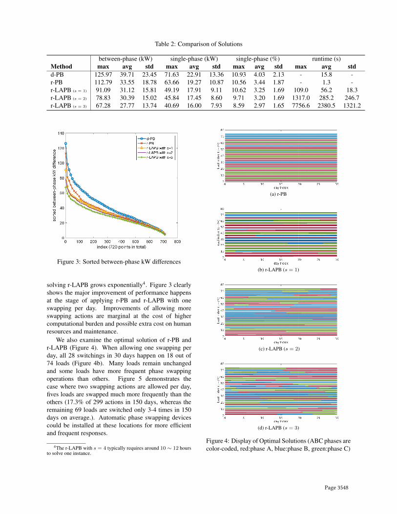
Table 2: Comparison of Solutions

between-phase (kW) single-phase (kW) single-phase (%) runtime (s)Method max avg std max avg std max avg std max avg stdd-PB 125.97 39.71 23.45 71.63 22.91 13.36 10.93 4.03 2.13 - 15.8 -r-PB 112.79 33.55 18.78 63.66 19.27 10.87 10.56 3.44 1.87 - 1.3 -r-LAPB (s = 1) 91.09 31.12 15.81 49.19 17.91 9.11 10.62 3.25 1.69 109.0 56.2 18.3r-LAPB (s = 2) 78.83 30.39 15.02 45.84 17.45 8.60 9.71 3.20 1.69 1317.0 285.2 246.7r-LAPB (s = 3) 67.28 27.77 13.74 40.69 16.00 7.93 8.59 2.97 1.65 7756.6 2380.5 1321.2

Figure 3: Sorted between-phase kW differences

solving r-LAPB grows exponentially4. Figure 3 clearlyshows the major improvement of performance happensat the stage of applying r-PB and r-LAPB with oneswapping per day. Improvements of allowing moreswapping actions are marginal at the cost of highercomputational burden and possible extra cost on humanresources and maintenance.

We also examine the optimal solution of r-PB andr-LAPB (Figure 4). When allowing one swapping perday, all 28 switchings in 30 days happen on 18 out of74 loads (Figure 4b). Many loads remain unchangedand some loads have more frequent phase swappingoperations than others. Figure 5 demonstrates thecase where two swapping actions are allowed per day,fives loads are swapped much more frequently than theothers (17.3% of 299 actions in 150 days, whereas theremaining 69 loads are switched only 3-4 times in 150days on average.). Automatic phase swapping devicescould be installed at these locations for more efficientand frequent responses.

4The r-LAPB with s = 4 typically requires around 10 ∼ 12 hoursto solve one instance.

(a) r-PB

(b) r-LAPB (s = 1)

(c) r-LAPB (s = 2)

(d) r-LAPB (s = 3)

Figure 4: Display of Optimal Solutions (ABC phases arecolor-coded, red:phase A, blue:phase B, green:phase C)

Page 3548

Figure 5: Phase Swapping Actions of Each Load (resultsof r-LAPB (s = 2) running for 150 days)

5. Discussions

5.1. Uncertainty Sets

In this paper, the uncertainty sets (13)-(14) weuse are a special case of polyhedral uncertainty sets.We do not capture yet potential correlations amongdifferent loads, as shown in Figure 2a. Other choicesof uncertainty sets might outperform current ones andreduce conservativeness, e.g. central limit theorembased polyhedral sets [22], ellipsoidal uncertainty sets[34], cardinality constrained uncertainty sets [35], andconstructing polyhedral uncertainty sets from data [36].

5.2. Approximation Algorithms

All our formulations of phase balancing problemsare mixed integer programs, which are in generalcomputationally intractable. One of the classicalproblems in combinatorial optimization is minimummakespan scheduling that attempts to run a given setof jobs on a fixed number of parallel machines suchthat total time, i.e. the makespan, to complete jobson any machine is minimized [37]. Minimizing themaximum total load on any phase can then be viewedas makespan scheduling where the given set of jobsis simply the various loads, and the three parallelidentical machines are the three phase lines. It is anopen question to adapt known approximation algorithmsfor the minimum makespan scheduling problem (or todevelop new methods) to the robust framework whileincorporating switching costs. Deterministic phasebalancing (d-PB) can also be seen as the optimizationversion of the k-partition problem [38], that attempts todivide n integers into k subsets such that the total sumof each subset is close to each other. This problem isa generalization of the three phase balancing problem,

and might provide useful insights as well.

5.3. Multi-phase Loads

It is easy to extend current phase balancing problemsfor the consideration of multi-phase loads. Fordeterministic phase balancing (6), we could definevariable a(1), b(1) and c(1) for single phase loads, a(2),b(2) and c(2) for two-phase loads, a(3), b(3) and c(3)

for loads connecting to all three phases. Instead ofconstraint (6e), we have the following constraints:

a(1) + b(1) + c(1) = 1,

a(2) + b(2) + c(2) = 2 · 1, anda(3) + b(3) + c(3) = 3 · 1.

6. Concluding Remarks

In this paper, we advance the conventional phasebalancing problem to a robust look-ahead optimizationframework that pursuits balanced phases in the presenceof uncertainties. It is shown that imbalances amongphases could be significantly reduced at the cost ofa limit number of phase swapping operations. Manyinteresting directions are open for future research.For example, choosing different uncertainty sets forr-LAPB could take advantage of strong correlationamong some loads. Future works also include designingapproximation algorithms with optimality guaranteesand exploring the benefits of controlling distributedgenerations [39–41], electric vehicles [42–44], energystorage [29, 45–47] and demand response [48–51].

Acknowledgement

This work was supported in part by Power SystemsEngineering Research Center (PSERC) and in part bythe Simons Institute for the Theory of Computing. Thiswork was partially done while the authors were visitingthe Simons Institute for the Theory of Computing, UCBerkeley, and we would like to acknowledge the Gordonand Betty Moore Foundation for their generous support.

A. Appendix: Equivalent Formulation ofRobust Look-ahead Phase Balancing

Formulation (11) is equivalent with the following:

minimize u+ λv (15a)

subject to hᵀt pa[t] ≤ u, Hᵀ

t pa[t] = a[t]− 1

3, (15b)

hᵀt qa[t] ≤ u, Hᵀ

t qa[t] =1

3− a[t], (15c)

Page 3549

hᵀt pb[t] ≤ u, Hᵀ

t pb[t] = b[t]− 1

3, (15d)

hᵀt qb[t] ≤ u, Hᵀ

t qb[t] =1

3− b[t], (15e)

hᵀt pc[t] ≤ u, Hᵀ

t pc[t] = c[t]− 1

3, (15f)

hᵀt qc[t] ≤ u, Hᵀ

t qc[t] =1

3− c[t], (15g)

t = 1, 2, · · · , T1,

hᵀt pa[t] ≤ v, Hᵀ

t pa[t] = a[T1]−1

3, (15h)

hᵀt qa[t] ≤ v, Hᵀ

t qa[t] =1

3− a[T1], (15i)

hᵀt pb[t] ≤ v, Hᵀ

t pb[t] = b[T1]−1

3, (15j)

hᵀt qb[t] ≤ v, Hᵀ

t qb[t] =1

3− b[T1], (15k)

hᵀt pc[t] ≤ v, Hᵀ

t pc[t] = c[T1]−1

3, (15l)

hᵀt qc[t] ≤ v, Hᵀ

t qc[t] =1

3− c[T1], (15m)

t = T1 + 1, T1 + 2, · · · , T2,

− wa[t] ≤ a[t]− a[t− 1] ≤ wa[t], (15n)

− wb[t] ≤ b[t]− b[t− 1] ≤ wb[t], (15o)

− wc[t] ≤ c[t]− c[t− 1] ≤ wc[t], (15p)

T1∑t=1

(1ᵀwa[t] + 1ᵀwb[t] + 1ᵀwc[t]

)≤ 2s,

(15q)

a[t] + b[t] + c[t] = 1, (15r)

a[t], b[t], c[t] ∈ {0, 1}n, u, v ∈ R+, (15s)

wa[t], wb[t], wc[t] ∈ Rn+ (15t)t = 1, 2, · · · , T1,

pa[t], pb[t], pc[t], qa[t], qb[t], qc[t] ∈ Rk+, (15u)

t = 1, 2, · · · , T2.

References

[1] J. Zhu, M.-Y. Chow, and F. Zhang, “Phase balancingusing mixed-integer programming [distributionfeeders],” IEEE transactions on power systems,vol. 13, no. 4, pp. 1487–1492, 1998.

[2] L. F. Ochoa, R. M. Ciric, A. Padilha-Feltrin, and G. P.Harrison, “Evaluation of distribution system losses dueto load unbalance,” in 15th PSCC, vol. 6, pp. 1–4, 2005.

[3] T.-H. Chen and J.-T. Cherng, “Optimal phasearrangement of distribution transformers connectedto a primary feeder for system unbalance improvementand loss reduction using a genetic algorithm,” in Power

Industry Computer Applications, 1999. PICA’99.Proceedings of the 21st 1999 IEEE InternationalConference, IEEE, 1999.

[4] K. Ma, R. Li, and F. Li, “Quantification of additionalasset reinforcement cost from 3-phase imbalance,”IEEE Transactions on Power Systems, vol. 31, no. 4,pp. 2885–2891, 2016.

[5] R. Yan and T. K. Saha, “Investigation of voltageimbalance due to distribution network unbalanced lineconfigurations and load levels,” IEEE Transactions onPower Systems, vol. 28, no. 2, pp. 1829–1838, 2013.

[6] F. Shahnia, P. J. Wolfs, and A. Ghosh, “Voltageunbalance reduction in low voltage feeders by dynamicswitching of residential customers among three phases,”IEEE Transactions on Smart Grid, vol. 5, no. 3,pp. 1318–1327, 2014.

[7] M. S. Modarresi, T. Huang, H. Ming, and L. Xie,“Robust phase detection in distribution systems,” inPower and Energy Conference (TPEC), IEEE Texas,pp. 1–5, IEEE, 2017.

[8] H. Xu, A. D. Domnguez-Garca, and P. W. Sauer,“A data-driven voltage control framework for powerdistribution systems,” in In Proceedings of 2018 Powerand Energy Society General Meeting (PESGM), IEEE,2018.

[9] “Voltage Security Constrained Look-ahead Coordinationof Reactive Power Support Devices with HighRenewables,” in Proceedings of the 19th InternationalConference on Intelligent System Applications to PowerSystems, author = Geng, Xinbo and Xie, Le andObadina, Diran, year = 2017.

[10] Xinbo Geng, Le Xie, and Diran Obadina,“Chance-constrained Optimal Reactive Power Dispatch,”in In Proceedings of 2018 Power and Energy SocietyGeneral Meeting (PESGM), IEEE, 2018.

[11] A. Khodabakhsh, G. Yang, S. Basu, E. Nikolova,M. C. Caramanis, T. Lianeas, and E. Pountourakis,“A Submodular Approach for Electricity DistributionNetwork Reconfiguration,” in Proceedings of the 36thAnnual Hawaii International Conference on SystemSciences, 2017, 2017.

[12] S. Civanlar, J. Grainger, H. Yin, and S. Lee,“Distribution feeder reconfiguration for loss reduction,”IEEE Transactions on Power Delivery, vol. 3, no. 3,pp. 1217–1223, 1988.

[13] J. Zhu, G. Bilbro, and M.-Y. Chow, “Phase balancingusing simulated annealing,” IEEE Transactions on PowerSystems, vol. 14, no. 4, pp. 1508–1513, 1999.

[14] C.-H. Lin, C.-S. Chen, H.-J. Chuang, M.-Y. Huang,and C.-W. Huang, “An expert system for three-phasebalancing of distribution feeders,” IEEE Transactions onPower Systems, vol. 23, no. 3, pp. 1488–1496, 2008.

[15] R. A. Hooshmand and S. Soltani, “Fuzzy optimal phasebalancing of radial and meshed distribution networksusing BF-PSO algorithm,” IEEE Transactions on PowerSystems, vol. 27, no. 1, pp. 47–57, 2012.

[16] C. Lin, C. Chen, M. Huang, H. Chuang, M. Kang,C. Ho, and C. Huang, “Optimal phase arrangementof distribution feeders using immune algorithm,” inIntelligent Systems Applications to Power Systems, 2007.ISAP 2007. International Conference on, pp. 1–6, IEEE,2007.

[17] K. Wang, S. Skiena, and T. G. Robertazzi, “Phasebalancing algorithms,” Electric Power Systems Research,vol. 96, pp. 218–224, 2013.

Page 3550

[18] M. Dilek, R. P. Broadwater, J. C. Thompson, andR. Seqiun, “Simultaneous phase balancing at substationsand switches with time-varying load patterns,” IEEETransactions on Power Systems, vol. 16, no. 4,pp. 922–928, 2001.

[19] C.-H. Lin, C.-S. Chen, H.-J. Chuang, and C.-Y. Ho,“Heuristic rule-based phase balancing of distributionsystems by considering customer load patterns,” IEEETransactions on Power Systems, vol. 20, no. 2,pp. 709–716, 2005.

[20] J. R. Birge and F. Louveaux, Introduction to stochasticprogramming. Springer Science & Business Media.

[21] D. Bertsimas and M. Sim, “The price of robustness,”Operations research, vol. 52, no. 1, pp. 35–53, 2004.

[22] C. Bandi and D. Bertsimas, “Tractable stochasticanalysis in high dimensions via robust optimization,”Mathematical programming, 2012.

[23] A. Ben-Tal, L. El Ghaoui, and A. Nemirovski, Robustoptimization. Princeton University Press, 2009.

[24] D. Bertsimas, D. B. Brown, and C. Caramanis, “Theoryand applications of robust optimization,” SIAM review,vol. 53, no. 3, pp. 464–501, 2011.

[25] A. Ben-Tal, L. El Ghaoui, and A. Nemirovski, Robustoptimization. Princeton University Press, 2009.

[26] A. A. Thatte, X. A. Sun, and L. Xie, “Robustoptimization based economic dispatch for managingsystem ramp requirement,” in System Sciences (HICSS),2014 47th Hawaii International Conference on,pp. 2344–2352, IEEE, 2014.

[27] L. Xie, Y. Gu, X. Zhu, and M. G. Genton,“Short-term spatio-temporal wind power forecast inrobust look-ahead power system dispatch,” IEEETransactions on Smart Grid, vol. 5, no. 1, pp. 511–520,2014.

[28] I. Gurobi Optimization, Gurobi Optimizer ReferenceManual. 2016.

[29] S. Sun, B. Liang, M. Dong, and J. A. Taylor, “Phasebalancing using energy storage in power grids underuncertainty,” IEEE Transactions on Power Systems,vol. 31, no. 5, pp. 3891–3903, 2016.

[30] A. Hoke, R. Butler, J. Hambrick, and B. Kroposki,“Steady-state analysis of maximum photovoltaicpenetration levels on typical distribution feeders,” IEEETransactions on Sustainable Energy, vol. 4, no. 2,pp. 350–357, 2013.

[31] K. P. Schneider, Y. Chen, D. P. Chassin, R. G. Pratt, D. W.Engel, and S. E. Thompson, “Modern grid initiativedistribution taxonomy final report,” tech. rep., PacificNorthwest National Laboratory (PNNL), Richland, WA(US), 2008.

[32] J. Lfberg, “Automatic robust convex programming,”Optimization methods and software, 2012.

[33] J. Lfberg, “YALMIP : A Toolbox for Modeling andOptimization in MATLAB,” in In Proceedings of theCACSD Conference, (Taipei, Taiwan), 2004.

[34] A. Ben-Tal and A. Nemirovski, “Robust solutions ofuncertain linear programs,” Operations research letters,vol. 25, no. 1, pp. 1–13, 1999.

[35] D. Bertsimas and M. Sim, “Robust discrete optimizationand network flows,” Mathematical programming,vol. 98, no. 1-3, pp. 49–71, 2003.

[36] D. Bertsimas, V. Gupta, and N. Kallus, “Data-drivenrobust optimization,” Mathematical Programming, 2018.

[37] J. K. Lenstra, D. B. Shmoys, and E. Tardos,“Approximation algorithms for scheduling unrelatedparallel machines,” Mathematical programming, vol. 46,no. 1-3, pp. 259–271, 1990.

[38] S. Sahni and T. Gonzalez, “P-complete approximationproblems,” Journal of the ACM (JACM), 1976.

[39] H. Xu, A. D. Domı́nguez-Garcı́a, and P. W. Sauer,“Adaptive coordination of distributed energy resourcesin lossy power distribution systems,” arXiv preprintarXiv:1711.04157, 2017.

[40] H. Xu, A. D. Domnguez-Garca, and P. W. Sauer,“Adaptive coordination of distributed energy resourcesin lossy power distribution systems,” in In Proceedingsof 2018 Power and Energy Society General Meeting,(Portland, OR), IEEE, 2018.

[41] H. Zhang, Z. Hu, E. Munsing, S. J. Moura, andY. Song, “Data-driven chance-constrained regulationcapacity offering for distributed energy resources,” IEEETransactions on Smart Grid, 2018.

[42] H. Zhang, Z. Hu, Z. Xu, and Y. Song, “Evaluation ofachievable vehicle-to-grid capacity using aggregate pevmodel,” IEEE Transactions on Power Systems, vol. 32,no. 1, pp. 784–794, 2017.

[43] H. Zhang, S. J. Moura, Z. Hu, W. Qi, and Y. Song, “Jointpev charging network and distributed pv generationplanning based on accelerated generalized bendersdecomposition,” IEEE Transactions on TransportationElectrification, 2018.

[44] X. Chen, H. Zhang, Z. Xu, C. P. Nielsen, M. B.McElroy, and J. Lv, “Impacts of fleet types and chargingmodes for electric vehicles on emissions under differentpenetrations of wind power,” Nature Energy, 2018.

[45] C. J. Bennett, R. A. Stewart, and J. W. Lu, “Developmentof a three-phase battery energy storage scheduling andoperation system for low voltage distribution networks,”Applied Energy, vol. 146, pp. 122–134, 2015.

[46] B. Xu, Y. Shi, D. S. Kirschen, and B. Zhang, “Optimalbattery participation in frequency regulation markets,”IEEE Transactions on Power Systems, 2018.

[47] B. Xu, J. Zhao, T. Zheng, E. Litvinov, and D. S.Kirschen, “Factoring the cycle aging cost of batteriesparticipating in electricity markets,” IEEE Transactionson Power Systems, vol. 33, no. 2, pp. 2248–2259, 2018.

[48] A. Haider, X. Geng, G. Sharma, L. Xie, andP. Kumar, “A control system framework for privacypreserving demand response of thermal inertial loads,”in 2015 IEEE International Conference on SmartGrid Communications (SmartGridComm), pp. 181–186,IEEE, 2015.

[49] A. Halder, X. Geng, P. Kumar, and L. Xie, “Architectureand Algorithms for Privacy Preserving Thermal InertialLoad Management by A Load Serving Entity,” IEEETransactions on Power Systems, 2016.

[50] B. Xia, H. Ming, K.-Y. Lee, Y. Li, Y. Zhou, S. Bansal,S. Shakkottai, and L. Xie, “Energycoupon: A case studyon incentive-based demand response in smart grid,” inProceedings of the Eighth International Conference onFuture Energy Systems, pp. 80–90, ACM, 2017.

[51] Hao Ming, Le Xie, Marco Campi, Simone Garatti,and P.R. Kumar, “Scenario-based Economic Dispatchwith Uncertain Demand Response,” accepted by IEEETransactions on Smart Grid, 2017.

Page 3551