Robust Impulsive Control of Motion Systems

with Uncertain Friction

Technical Report DC2010.031

N. van de Wouw⋆, R.I. Leine‡

⋆ Department of Mechanical Engineering,Eindhoven University of Technology,P.O. Box 513, 5600 MB Eindhoven,

The Netherlands,N.v.d.wouw@tue.nl

‡ Institute of Mechanical Systems,Department of Mechanical and Process

Engineering,ETH Zurich, CH-8092 Zurich, Switzerland

remco.leine@imes.mavt.ethz.ch

Abstract

In this paper, we consider the robust set-point stabilisation problem for motion systemssubject to friction. Robustness aspects are particularly relevant in practice, where uncertain-ties in the friction model are unavoidable. We propose an impulsive feedback control designthat robustly stabilises the set-point for a class of position-, velocity- and time-dependentfriction laws with uncertainty. Moreover, it is shown that this control strategy guarantees thefinite-time convergence to the set-point which is a favourable characteristic of the resultingclosed loop from a transient performance perspective. The results are illustrated by means ofa representative motion control example.

Key words: Robust Stabilisation, Impulsive Control, Friction, Motion Control.

1 Introduction

In this paper, we consider the robust set-point stabilisation problem for motion control systemswith uncertain friction using an impulsive control strategy. It is well known that controlled motionsystems with friction exhibit many undesirable effects such as stick-slip limit cycling, large settlingtimes and non-zero steady-state errors, see e.g. [3, 4, 6, 7, 11, 21, 23, 27]. In the literature manydifferent approaches towards the control of motion systems with friction have been proposed, suchas PID control design, friction compensation, dithering-based approaches, adaptive techniquesand impulsive control strategies. As shown e.g. in [3, 11], PID control techniques may sufferfrom an instability phenomenon known as hunting limit cycling. Many friction compensationapproaches are available in the literature (see, for example, [3, 7, 11, 17, 21, 23, 27, 29]) and havesuccessfully been applied in practice, although it is widely recognised that the undercompensationand overcompensation of friction (due to inevitable friction modelling errors) may lead to non-zerosteady-state errors and limit cycling [2,26,27]. Examples of adaptive compensation approaches arean adaptive friction compensation strategy reported in [25] and a model reference adaptive controlscheme proposed in [30]. Dithering-based approaches, see e.g. [3,15,16,31], aim at smoothing thediscontinuity induced by (Coulomb) friction by the introduction of high-frequency excitationsand thereby aim to avoid non-zero steady-state errors. The basic idea behind impulsive controlstrategies is the introduction of controlled impulsive forces when the system gets stuck at a non-zero steady-state error (due the stiction effect of friction), see e.g. [3,4,10,12–14,18,19,24,28,32–34].One of the key practical problems faced in any of those ‘friction-beating’ strategies is the fact thatfriction is a phenomenon which is particularly hard to model accurately, especially due to e.g.changing environmental conditions such as lubrication conditions, temperature, wear, humidity

1

etc. [3, 7, 23]. It is therefore of the utmost importance to develop stabilising controllers that arerobust against uncertainties in the friction.

Here, we propose an impulsive feedback control strategy which guarantees the robust sta-bility of the set-point in the face of frictional uncertainties, where we consider a large class ofposition-dependent, velocity-dependent, and time-varying friction models. The practical feasi-bility of impulsive force manipulation for the positioning of motion control systems has beenillustrated in [10, 12–14, 18, 28, 32, 33]. Moreover, different impulsive feedback control strategieshave been proposed in [18,19,24,32]. However, rigorous stability analyses of the closed-loop systemare rare, especially when accounting for uncertainties in the friction model. A notable exceptionis the recent work in [24] in which an impulsive feedback law similar to the one proposed in thispaper has been studied. The common idea behind this impulsive control law is that, when thesystem reaches the stick phase at a non-zero regulation error, an impulsive force is applied, whichkicks the system out of the stick phase and whose magnitude is dependent on the positioningerror. The current work differs from and extends the work in [24] in the following ways. Firstly, inthis paper we provide a proof for the robust set-point stability for a class of set-valued Coulombfriction models where the friction coefficient may be position-dependent, velocity-dependent andtime-dependent, whereas in [24] only a stability analysis for uncertain, but constant, friction co-efficients is given. Given the fact that position-dependencies, velocity-dependencies (think of e.g.the Stribeck effect) and time-dependent frictional characteristics (due to e.g. changing temper-ature, humidity or lubrication conditions) are always present in practice, such an extension isvery relevant for applications. Secondly, in [24] a combination of an impulsive controller with asmooth linear position-error feedback controller is considered. In the current work, we consideran impulsive controller in combination with a more general linear state-feedback controller. Asalso stated in [24], such an extension is highly desirable from a performance perspective. Finally,in the current paper we provide a proof for the finite-time stability of the set-point, as opposed tomere asymptotic stability in [24].

Resuming, the main contributions of the current paper are as follows. Firstly, we propose animpulsive feedback control design for a motion control system consisting of a controlled inertia sub-ject to friction modelled by a general class of set-valued, position-dependent, velocity-dependent,and time-varying friction models. Secondly, a stability analysis is performed to guarantee therobust stability of the set-point in the face of uncertainties in the friction. Thirdly, we show thatthe stability achieved is symptotic (i.e. attractivity in finite time to the set-point is guaranteed).

The outline of the paper is as follows. In Section 2, the control problem tackled in this paperis formalised. In Section 3, the impulsive control design is introduced. The robust (finite-time)stability analysis of the impulsive closed-loop system is presented in Section 4. The effectivenessof the control design and its robustness properties are illustrated by means of an example inSection 5. Finally, concluding remarks are presented in Section 6. Some of the proofs are collectedin the appendix.

2 Control Problem Formulation

Consider a one-degree-of-freedom mechanical system consisting of an inertia with mass m whichis in frictional contact with a support, being a flat horizontal plane (see Figure 1). We denotethe position of the inertia by z and its velocity by z whenever it exists. A friction force Ff actsbetween the mass and the support under the influence of a normal force mg, where g denotes thegravitational acceleration. The control input consist of a finite control force u and an impulsivecontrol force U . The dynamics of the control system is described by the equation of motion (thebalance of linear momentum)

mz = u + Ff (z, z, t) (1)

and the impact equation

m(z+(tj) − z−(tj)) = U, (2)

2

which relates the difference between the post-impact velocity z+(tj) and the pre-impact velocityz−(tj) to the impulsive control force U at time tj . It is tacitly assumed that the impulsive forceU is such that the velocity z(t) is of locally bounded variation. A proof for the validity of thisassumption can be found in Appendix A.

Figure 1: Mechanical motion system with control input.

The friction force Ff (z, z, t) is assumed to obey the following set-valued force law:

Ff (z, z, t) ∈ −mgµ(z, z, t)Sign(z), (3)

where Sign(·) denotes the set-valued sign function defined by

Sign(y) ,

−1, y < 0[−1, 1] , y = 01, y > 0

. (4)

Moreover, µ(z, z, t) denotes the friction coefficient that may depend on z and z, which are bothfunctions of time, and may also depend explicitly on time t. Note that (3) represent a ratherlarge class of friction models including possibly position-dependent friction, velocity-dependenteffects, such as the Stribeck effect, and time-dependent friction (which can occur in practicedue to changing temperature/humidity of the contact, wear or changing lubrication conditions).Moreover, (3) represents a set-valued friction model to account for the stiction effect induced by dryfriction. Despite the fact that (3) represents a static friction model, the explicit time-dependencycan also account for certain effects encountered in dynamic friction models. In the remainder ofthis paper, we adopt the following assumption on the friction coefficient.

Assumption 1

The friction coefficient µ(z, z, t) is lower bounded by µ and upper bounded by µ, i.e. it holds that

µ ≤ µ(z, z, t) ≤ µ, ∀t, z, z ∈ R, (5)

for some 0 < µ ≤ µ.

In the remainder of this paper, we express the dynamics of the system in first-order form byusing the state vector x = [x1 x2]

T:= [z z]

T. The impulsive and non-impulsive dynamics of

the system can be represented by a (in general non-autonomous) first-order measure differentialinclusion [1, 20, 22]:

dx1 = x2 dt

dx2 ∈ −gµ(x1, x2, t)Sign(x2) dt +1

mdp,

(6)

where

dp = u dt + U dη (7)

is the differential measure of the control input, dt is the Lebesgue measure and dη is a differentialatomic measure consisting of a sum of Dirac point measures [9, 20]. The decomposition of the

3

control force as in (7) implies that the differential measure dx of the state can be decomposed asfollows dx = x dt + (x+ − x

−) dη. Such a decomposition, implies that x(t) is a special functionof locally bounded variation [1]. The state x(t) admits at each time-instant t a left and right limitx−(tj) = limt↑tj

x(t), x+(tj) = limt↓tj

x(t), as x(t) is of (special) locally bounded variation. Thetime-evolution of x(t) is governed by the integration process x

+(t1) = x−(t0) +

∫

[t0,t1]dx, where

[t0, t1] denotes the compact time-interval between t0 and t1 ≥ t0.Now let us state the control problem considered in this paper:

Problem 1

Design a control law for u and U for system (6), (7) such that x = 0 is a robustly globallyuniformly attractively stable equilibrium point of the closed-loop system for a class of uncertainfriction models of the form (3) satisfying Assumption 1.

The attraction in Problem 1 can be asymptotic or symptotic, with which we mean attraction tothe equilibrium in infinite or finite time, respectively. The controller proposed in this paper willinduce stability and finite-time attractivity, i.e. symptotic stability1.

3 Impulsive Feedback Control Design

In order to solve Problem 1, we adopt a proportional-derivative (state-)feedback control law for uin (7) of the form

u(x1, x2) = −k1x1 − k2x2, k1, k2 > 0, (8)

together with an impulsive feedback control law for U in (7) of the form

U(x1, x−2 ) =

k3(x1), if (x−

2 = 0) ∧ (|x1| ≤ mgµk1

)

0, else, (9)

where the constants k1, k2 and the function k3(x1) are to be designed. The resulting closed-loopdynamics can be formulated in terms of a measure differential inclusion:

dx1 = x2 dt

dx2 ∈(

−k1

mx1 −

k2

mx2 − gµ(x1, x2, t)Sign(x2)

)

dt +1

mU(x1, x

−2 ) dη.

(10)

In between impulsive control actions, the non-impulsive dynamics is described by the differentialinclusion

x1 = x2

x2 ∈ −k1

mx1 −

k2

mx2 − gµ(x1, x2, t)Sign(x2).

(11)

The state of the system may jump at impulsive time-instants tj for which U 6= 0, i.e. for timeinstants at which

x−2 (tj) = 0, |x1(tj)| ≤

mgµ

k1, (12)

according to the state reset map

x+1 (tj) = x−

1 (tj)

x+2 (tj) = x−

2 (tj) +k3(x

−1 (tj))

m.

(13)

In the remainder we will denote x1(tj) = x−1 (tj) = x+

1 (tj) since the position x1(t) = z(t) is anabsolutely continuous function of time.

1For a definition of symptotic stability we refer to e.g. [20]

4

3.1 Analysis of the Non-impulsive Closed-loop Dynamics

In this section, we study properties of the solutions of the non-impulsive closed-loop dynamicsdescribed by the differential inclusion (11) that are important for the stability analysis pursued inSection 4.

If x2(t) 6= 0, then the differential inclusion (11) reduces to the nonlinear differential equation

x1 = x2

x2 = −k1

mx1 −

k2

mx2 ± gµ(x1, x2, t).

(14)

In the following we will regard the nonlinear term gµ(x1, x2, t) to be a time-varying input gµ(t)with µ(t) := µ(x1(t), x2(t), t), which obeys Assumption 1, i.e. µ ≤ µ(t) ≤ µ ∀t. Hence, theclosed-loop non-impulsive dynamics for x2(t) 6= 0 is described by the linear differential equation

x1 = x2

x2 = −ω2nx1 − 2ζωnx2 + f(t),

(15)

with time-varying input f(t) := −gµ(t)Sign(x2(t)), undamped eigenfrequency ωn =√

k1/m, and

damping ratio ζ = k2

2√

k1m> 0 and gµ ≤ f(t) ≤ gµ ∀t. Consider the case that the controller

parameters k1, k2 are designed such that ζ > 1. Denote λ1 := −ωnζ + ωn

√

ζ2 − 1, λ2 :=

−ωnζ −ωn

√

ζ2 − 1, and note that λ1λ2 = ω2n, λ1 + λ2 = −2ζωn and λ2 < λ1 < 0. We denote the

arbitrary initial condition as

x1(t0) = x10, x2(t0) = x20. (16)

Let (x1(t), x2(t)) denote the solution of the initial value problem (15), (16) on a time intervalfor which x2(t) does not change sign. Furthermore, let (x1(t), x2(t)) denote the solution of theinitial value problem (15), (16) for µ(t) = µ, ∀t and (x1(t), x2(t)) for µ(t) = µ, ∀t. The followingproposition explicates that xi(t) and xi(t) characterise bounds on xi(t) (i = 1, 2). Herein, we usethe following definitions:

c :=mgµ

k1=

gµ

λ1λ2, c :=

mgµ

k1=

gµ

λ1λ2. (17)

Proposition 1

The solutions (x1(t), x2(t)) and (x1(t), x2(t)) satisfy

x1(t) = s1(t − t0)x10 + s2(t − t0)x20 − c (1 − s1(t − t0)) ,

x2(t) = s1(t − t0)x10 + s2(t − t0)x20 − λ1λ2c s2(t − t0)(18)

and

x1(t) = s1(t − t0)x10 + s2(t − t0)x20 − c (1 − s1(t − t0)) ,

x2(t) = s1(t − t0)x10 + s2(t − t0)x20 − λ1λ2c s2(t − t0)(19)

with the definitions for c and c as in (17) and s1(t), s2(t) defined by

s1(t) =λ2

λ2 − λ1eλ1t − λ1

λ2 − λ1eλ2t, and s2(t) =

1

λ2 − λ1

(−eλ1t + eλ2t

). (20)

Moreover, the solution (x1(t), x2(t)) is lower and upper bounded by the solutions (x1(t), x2(t))and (x1(t), x2(t)) according to

x2 > 0 : x1(t) ≤ x1(t) ≤ x1(t), x2(t) ≤ x2(t) ≤ x2(t) for 0 ≤ t − t0 ≤ 1

λ2 − λ1ln

λ1

λ2,

x2 < 0 : x1(t) ≥ x1(t) ≥ x1(t), x2(t) ≥ x2(t) ≥ x2(t) for 0 ≤ t − t0 ≤ 1

λ2 − λ1ln

λ1

λ2.

(21)

Proof The proof is given in Appendix B.

5

3.2 Impulsive Controller Design

Let us first explain the rationale behind the design of the controller (7), (8), (9). Hereto, considerthe case that µ(x1, x2, t) = µ, with µ a constant, and consider the system without the impulsivepart of the controller (i.e. k3(x1) = 0 in (9)). In this case the closed-loop system is a PD-controlledinertia with Coulomb friction which exhibits an equilibrium set defined by x ∈ R

2 | |x1| ≤mgµk1

∧ x2 = 0. Clearly, the closed-loop system will then ultimately converge to the equilibriumset and an undesirable non-zero steady-state error will in general result. This attraction caneither occur in a finite time or the solution can approach the equilibrium set asymptotically [5,8].Note that for (non-constant) friction coefficients µ(x1, x2, t) satisfying Assumption 1, the closed-loop system without impulsive control will exhibit a time-varying stick set E(t) that satisfiesE ⊆ E(t) ⊆ E ∀t, where E = x ∈ R

2 | |x1| ≤ mgµ

k1∧x2 = 0, E = x ∈ R

2 | |x1| ≤ mgµk1

∧x2 = 0are the minimal and maximal stick sets, respectively. A point x

∗ ∈ E remains stationary for alltimes and is therefore an equilibrium point of the PD-controlled system. The time-varying natureof the stick set E(t) may destroy the stationarity of points in E(t)\E . The set E(t) thereforedenotes the stick set at time t and not an equilibrium set. The basic idea behind the impulsivecontroller (7), (8), (9) is to apply an impulsive control force when the state of the system enters themaximal stick-set E . Loosely speaking, the impulsive force kicks the system out off the stick phaseallowing it to further converge (closer) to the set-point. Since the friction law is uncertain alsothe stick set E(t) is not known a priori and the closed-loop system without impulsive control mayeven get stuck at zero velocity temporarily when µ(z, z, t) is indeed time-dependent. To enforcethat the system never remains at zero velocity for more than an isolated time instant (i.e. for atime interval of positive Lebesgue measure), we design the impulsive controller in (9) such thatan impulsive force is applied whenever x

−(t) ∈ E . Clearly, the impulsive part of the controllerprevents the existence of an equilibrium set (and the occurrence of non-zero steady-state errors).However, energy will be added to the system at every time-instant on which an impulsive controlaction is applied. In this paper, we will provide design rules for k1, k2 and k3(x1) such that moreenergy is dissipated (through the derivative action of the controller and the friction) in a time-interval between two impulsive control actions than is provided by the impulsive control actionpreceding this time-interval.

In order to design the impulsive part of the controller k3(x1), we take the following perspective.Consider a time instant tj for which x

−(tj) ∈ E , i.e. an impulsive control action U = k3(x1(tj))will be induced by the controller (7) at t = tj . Note that an impulsive control force results onlyin a jump of the velocity x2(t) whereas the position x1(t) is absolutely continuous, as formalisedin (13). The impulsive control action will cause x

+(tj) /∈ E . Let tj+1 denote the first time-instantfor which x(t) reaches again E , i.e. x−

2 (tj+1) = 0. Now, we will design k3(x1) in (9)such thatthe velocity will be reset to such a post-impact velocity x+

2 (tj) that the solution to (11), withµ(z, z, t) = µ and initial condition

(x1(tj), x

+2 (tj)

), will converge to the origin in finite time tj+1

without any impulses and/or velocity reversals occurring in the time-interval (tj , tj+1]. So, the(impulsive) controller is designed such that it stabilises the setpoint in finite time with only oneimpulsive action when the friction coefficient equals its lower bound. The impulsive controllerdesign will satisfy the condition

k3(y) =

< 0, y > 0

= 0, y = 0

> 0, y < 0

; (22)

in other words, x = 0 is an equilibrium point of the controlled system and the impulsive controlforce U is opposite to the position error x1(tj), which appeals to our intuition. In Section 4, we willshow that this control design also robustly stabilises the closed-loop system with a time-varyingand state-dependent friction coefficient µt = µ(x1(t), x2(t), t) satisfying Assumption 1.

Let us now design the impulsive control law k3(x1) that has the above properties. Hereto,consider the case that x1(tj) < 0 (the case x1(tj) > 0 can be studied in an analogous fashion).This implies that k3(x1(tj)) > 0, see (22), and x+

2 (tj) > 0. On the non-impulsive open time-

6

interval (tj , tj+1), the dynamics of (6) for µ(x1, x2, t) = µ is therefore governed by the differentialequation (15) with ζ > 1 and f(t) = fconst = −gµ, i.e.

x1(t) = x2(t)

x2(t) = −ω2nx1(t) − 2ζωnx2(t) − gµ.

(23)

We seek a solution curve of (23) with the boundary conditions x+(tj) =

[

x1(tj) x+2 (tj)

]T

and

x−(tj+1) =

[

0 0]T

. The initial position x1(tj) and initial time tj are a priori known. The initial

velocity x+2 (tj) as well as the end time tj+1 > tj are yet unknown. We therefore have to solve a

kind of mixed boundary value problem for the unknowns x+2 (tj) and tj+1. The boundary value

problem can be solved in many different ways. The rationale behind the method which we proposehere is to arrive at an algebraic equation for which we can prove the existence and uniquenessof the solution. We can express the solution for µ(x1, x2, t) = µ in closed form using the general

solution (18) by taking tj+1 = t0 as reference time and x10 = x1(tj+1) = 0, x20 = x−2 (tj+1) = 0,

which gives

x1(t) = −c(1 − s1(t − tj+1)

)= c

(λ2

λ2 − λ1eλ1(t−tj+1

) − λ1

λ2 − λ1eλ2(t−tj+1

) − 1

)

,

x2(t) = −λ1λ2c s2(t − tj+1) = cλ1λ2

λ2 − λ1

(

eλ1(t−tj+1) − eλ2(t−tj+1

))

,

(24)

with c given by (17).Subsequently, using (24) we require that x1(t) at time tj equals the a priori known initial positionx1(tj). This yields a nonlinear real algebraic equation

f(tj+1) = 0 (25)

for the unknown end time tj+1, where the function f(t) is given by

f(t) := c (s1(tj − t) − 1) − x1(tj) = c

(λ2

λ2 − λ1eλ1(tj−t) − λ1

λ2 − λ1eλ2(tj−t) − 1

)

− x1(tj). (26)

We can easily verify that f(tj) = −x1(tj) > 0 holds.Let us now study the following questions for the system of equations (24), (25), (26):

• For which domain in x1(tj) does a solution pair (tj+1, x+2 (tj)) exist (and can we show the

uniqueness of this solution)?

• If a such solution pair exists, can we show that both the time lapse tj+1 − tj and x+2 (tj) are

bounded for bounded x1(tj) (i.e. the impulsive control law yields bounded impulses and theresulting flowing response of system (23) converges to the origin in finite time)?

In the following proposition, we propose the impulsive control law and show that it exhibits theabove properties. Note that the impulsive control action k3(x1(tj)) can be computed from (13)using the fact that x−

2 (tj) = 0:

k3(x1(tj)) = mx+2 (tj). (27)

Proposition 2

Consider the impulsive control law k3(x1(tj)) for a given x1(tj), with tj arbitrary, defined by (27),where

1. tj+1 is the solution of (25), (26);

2. the value of x+2 (tj) is determined by the evaluation of x2(t), given by (24) at t = tj .

7

If ζ > 1, then it holds that k3(x1) is uniquely defined and bounded for all (x1, x2) ∈ E .

Proof The proof is given in Appendix B.

Note that the impulsive control law (27) can be computed a priori given the plant properties, suchas the mass m, the uncertainty bounds µ and µ on the friction coefficient, the gains k1 and k2 ofthe PD-controller and the gravitational acceleration g.

3.2.1 Characteristics of the impulsive control law

In this section, we further illuminate particular characteristics of the impulsive control law k3(x1)designed above. These characteristics will be exploited in Section 4 to study the stability of theimpulsive closed-loop system.

It holds that x+2 (tj) = −f

′(tj+1) and we can therefore writedx+

2(tj)

dtj+1

= −f′′(tj+1). Moreover,

differentiation of the algebraic equation f(tj+1; x1(tj)) = 0, in which with some abuse of notationwe make explicit that f also depends on x1(tj), using ∂f/∂x1(tj) = −1, yields

f′(tj+1) dtj+1 − dx1(tj) = 0 =⇒

dtj+1

dx1(tj)=

1

f′(tj+1). (28)

Consequently, the impulsive control law k3(x1(tj)) has a slope given by

dk3(x1(tj))

dx1(tj)= m

dx+2 (tj)

dx1(tj)= m

dx+2 (tj)

dtj+1

dtj+1

dx1(tj)= −m

f′′(tj+1)

f′(tj+1), (29)

or, using f′(tj+1) = −x+

2 (tj) = −k3(x1(tj))/m, by k′3(x1(tj)) = m2 f

′′(tj+1

)

k3(x1(tj)). For ζ > 1, it holds

that f′′(tj+1) ≤ −cω2

n −λ2f′(tj+1) for all tj+1 ≥ tj . We therefore obtain the differential inequality

k′3(y) ≤ mλ2 −

cω2nm2

k3(y), (30)

on the domain y < 0 with the boundary condition k3(0) = 0. The differential equation h′ = −a/hwith h(0) = 0 has the solution h(x) =

√−2ax on the domain x ≤ 0. The impulsive control law

k3(y) is therefore bounded from below by

k3(y) ≥√

−2cω2nm2y, y ≤ 0, (31)

as well as by k3(y) ≥ mλ2y, for y ≤ 0. The symmetry of the problem implies the unevenness ofk3(y), i.e. k3(y) = −k3(−y), and we therefore obtain

k3(y) ≤ −√

2cω2nm2y, y ≥ 0. (32)

Moreover, for small values of |y| the impulsive control law k3(y) can be well approximated by

k3approx(y) = − sign(y)√

2cω2nm2|y| (33)

because if y ↑ 0 then tj+1 ↓ tj and f′′(tj+1) ↑ −cω2

n. Hence if ζ > 1, then the slope k′3(y) is negative

for all y 6= 0, but is tending to minus infinity for y → 0. The graph of the impulsive control lawk3(y), which is a continuous uneven function, is therefore strictly decreasing for ζ > 1 and is locallysimilar to the square-root function k3approx(y) around the origin. A schematic representation ofthe impulsive control law k3(x1) for ζ > 1 is given in Figure 2, where we recall that it is only

applied for x1 ∈ E∗= x1 ∈ R | |x1| ≤ mgµ

k1 (the solid part of the graph).

The characteristics of the impulsive control explicated in (31), (32) and (33) will be used inProposition 6, which, in turn, plays a key role in the stability analysis in Section 4.

8

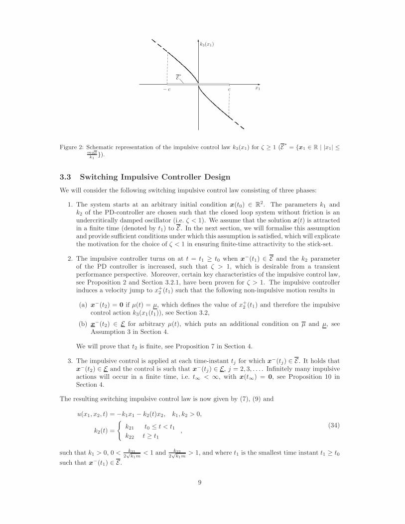
Figure 2: Schematic representation of the impulsive control law k3(x1) for ζ ≥ 1 (E∗

= x1 ∈ R | |x1| ≤mgµ

k1).

3.3 Switching Impulsive Controller Design

We will consider the following switching impulsive control law consisting of three phases:

1. The system starts at an arbitrary initial condition x(t0) ∈ R2. The parameters k1 and

k2 of the PD-controller are chosen such that the closed loop system without friction is anundercritically damped oscillator (i.e. ζ < 1). We assume that the solution x(t) is attractedin a finite time (denoted by t1) to E . In the next section, we will formalise this assumptionand provide sufficient conditions under which this assumption is satisfied, which will explicatethe motivation for the choice of ζ < 1 in ensuring finite-time attractivity to the stick-set.

2. The impulsive controller turns on at t = t1 ≥ t0 when x−(t1) ∈ E and the k2 parameter

of the PD controller is increased, such that ζ > 1, which is desirable from a transientperformance perspective. Moreover, certain key characteristics of the impulsive control law,see Proposition 2 and Section 3.2.1, have been proven for ζ > 1. The impulsive controllerinduces a velocity jump to x+

2 (t1) such that the following non-impulsive motion results in

(a) x−(t2) = 0 if µ(t) = µ, which defines the value of x+

2 (t1) and therefore the impulsivecontrol action k3(x1(t1)), see Section 3.2,

(b) x−(t2) ∈ E for arbitrary µ(t), which puts an additional condition on µ and µ, see

Assumption 3 in Section 4.

We will prove that t2 is finite, see Proposition 7 in Section 4.

3. The impulsive control is applied at each time-instant tj for which x−(tj) ∈ E . It holds that

x−(t2) ∈ E and the control is such that x

−(tj) ∈ E , j = 2, 3, . . . . Infinitely many impulsiveactions will occur in a finite time, i.e. t∞ < ∞, with x(t∞) = 0, see Proposition 10 inSection 4.

The resulting switching impulsive control law is now given by (7), (9) and

u(x1, x2, t) = −k1x1 − k2(t)x2, k1, k2 > 0,

k2(t) =

k21 t0 ≤ t < t1

k22 t ≥ t1,

(34)

such that k1 > 0, 0 < k21

2√

k1m< 1 and k22

2√

k1m> 1, and where t1 is the smallest time instant t1 ≥ t0

such that x−(t1) ∈ E .

9

4 Stability Analysis

In the previous section, we have introduced the switching impulsive control design. In this section,we will show that this control design symptotically (finite-time) stabilises the set-point x = 0.Consider the system (6) satisfying Assumption 1 and the impulsive feedback controller (7), (9), (34)with k3(x1) satisfying (27) and x+

2 (tj) fulfilling the mixed boundary value problem (see point 2in Proposition 2). In the following we will call this the resulting closed-loop system. We willprove that x = 0 is a globally uniformly symptotically stable equilibrium point of the resultingclosed-loop system.

Let us first prove boundedness of solutions.

Proposition 3

The solutions of the resulting closed-loop system (6), (7), (9), (34), satisfying Assumption 1, arebounded.

Proof The proof is given in Appendix B.

Secondly, let us assume that solutions which start in x(t0) ∈ R2 reach the compact set E in a

finite time t1.

Assumption 2

Solutions of the resulting closed-loop system (6), (7), (9), (34), satisfying Assumption 1, which

start in x(t0) ∈ R2 reach the compact set E in a finite time t1 (i.e. t1 − t0 < ∞).

We now formulate two sufficient conditions for Assumption 2 in the following two propositions.

Proposition 4

Suppose the friction coefficient µ(x1, x2, t) satisfies Assumption 1. If the time-evolution of thefriction coefficient µ(t) = µ(x1(t), x2(t), t) along solutions of the closed-loop system (6), (7), (34),with U = 0, is piecewise constant, such that it is constant during each time-interval for whichx2(t) does not change sign, and the linear part of the closed loop system is undercritically damped(i.e. ζ < 1), then the stick set E is reached in finite time for any initial condition x(t0) ∈ R

2.

Proof In [8], Theorem 2(iii), finite-time attraction is proven for a constant value of µ(t). Theproof can easily be extended to a piecewise constant µ(t) as in the proposition.

Proposition 5

Consider the closed-loop system (6), (7), (34), with U = 0. Consider a velocity-dependent frictionlaws satisfying the decomposition Ff (x2) ∈ −mgµ Sign(x2) − Fsm(x2) instead of the friction lawin (3), where µ is constant and satisfies Assumption 1, Fsm(·) ∈ C1 and Ff (x2)x2 ≤ 0, ∀x2. If

k21 +∂Fsm

∂x2(0) < 2

√

mk1, (35)

i.e. the linearisation of the continuous part of the closed-loop dynamics (around the origin) isundercritically damped, then the stick set E is reached in finite time for any initial conditionx(t0) ∈ R

2.

Proof Under the conditions in the proposition, Theorem 2 in [8] can be directly employed toprovide the proof.

Remark 1

Given the rather generic class of friction laws considered in this paper, the condition on thefriction law in Propositions 4 and 5 can be considered to be restrictive. Note, however, that(possibly asymmetric) Coulomb friction laws with uncertain (though constant) friction coefficientform a practically relevant subclass of friction models that satisfies the conditions in Proposition 4

10

and that the friction law in Proposition 5 represents a general class of discontinuous, velocity-dependent friction laws (possibly including the Stribeck effect). Moreover, the formulation of lessstringent conditions for the finite-time convergence to the stickset for the case of generic frictioncoefficients µ(x1, x2, t) is, to the best the authors’ knowledge, an open problem. Namely, it hasbeen shown in [5,8] that, even for constant µ, manifolds in state space may exist for which solutionsonly converge to the equilibrium set asymptotically (not in finite time). More precisely, in [8], it isshown that under the conditions in Proposition 5 with k21+ ∂Fsm

∂x2(0) ≥ 2

√mk1, solutions exist that

reach the equilibrium set in infinite time. Based on Propositions 4 and 5 and the work in [8], [5],we conclude that the fact that the linearised dynamics is undercritically damped appears to bean essential condition for the finite-time attractivity of the equilibrium set. This is the reason fordesigning the switching controller as in (34).

We do stress here that, although more generic sufficient conditions for Assumption 2 arecurrently lacking, it has been widely observed in the literature (both on a model level as inexperiments), see e.g. [3,21,27], that solutions in practice generally do converge to the stickset infinite time. In fact, this finite-time convergence to the stick set is directly related to the problemsof stick-slip limit cycling and non-zero steady-state errors, which we are aiming to tackle with thecontrol design in this paper and form the core motivation for our work. Hence, from a practicalpoint of view, Assumption 2 is a very natural one.

Remark 2

Let us consider an alternative tuning for the switching state-feedback controller in (34) such that

also the position feedback gain is switched according to k1 = 0, for t0 ≤ t ≤ t1, k1 ≤ mgµ|x1(t1)| , for

t ≥ t1 and the velocity feedback gain k2 > 0 is taken constant and such that ζ > 1 for t ≥ t1.In this case it is straightforward to show that for general µ(x1, x2, t), satisfying Assumption 1,Assumption 2 is satisfied. Still, we prefer to use the design proposed in (34) since the abovealternative control design leads to position feedback gains dependent on the initial conditions,which may lead to unpredictable/inferior transient performance.

Using the arguments and assumptions above we can now consider initial conditions (at t = t1)

satisfying x−(t1) =

[x1(t1) x−

2 (t1)]T ∈ E−

:= x ∈ E | x1 < 0. The case in which x1 > 0 can betreated in an entirely analogous fashion. Now, we consider a sequence of time instants tj, j ≥ 1,

such that x−(tj) ∈ E−

and x(t) 6∈ E−for t 6= tj . Clearly, due to the design of the impulsive part

of the control law as in (9), an impulse will now be applied instantly at t = tj and the system

undergoes a state reset to x+(tj) =

[x1(tj) x+

2 (tj)]T

= [x1(tj) k3(x1(tj))/m]T, see (13). We will

show below that if x1(t1) < 0, then x1(tj) ≤ 0, ∀j ≥ 1. Note that for x1(tj) < 0 we have thatx+

2 (t1) > 0, since x1(tj)k3(x1(tj)) < 0. Now, we study solutions flowing from x+(tj) until they

reach again the set E . We denote the next time instants at which these solutions reach E by tj+1,tj+1 and tj+1 for µ = µ(x1, x2, t), µ = µ and µ = µ, respectively. In doing so, we consider threedifferent systems:

1. system (15) with f(t) = −gµ(x1(t), x2(t), t) and solution x(t) on (tj , tj+1),

2. system (15) with f(t) = −gµ, i.e. system (23), and solution x(t) on (tj , tj+1),

3. system (15) with f(t) = −gµ and solution x(t) on (tj , tj+1).

All three solutions x(t), x(t) and x(t) have the same initial condition and are sketched in Figure 3.By Γµ we denote the solution segment x(t), for t ∈

(tj , tj+1

), and by Γµ we denote the solution

segment x(t), for t ∈(tj , tj+1

). By χ we denote the set enclosed by the line segments Γµ, Γµ,

and the axis x2 = 0 (gray set in Figure 3). A solution x(t) which starts in the set χ can not crossΓµ or Γµ. So, the solution x(t) is confined between Γµ and Γµ and if it leaves χ then this canonly happen through the line x2 = 0. However, for an arbitrary initial condition, it might alsobe that the solution approaches the edge of E(t) asymptotically and therefore never leaves χ (weonce more recall the results in [5, 8]). We first show that for µ(t) = µ solutions which start in Ereturn to E in a finite time and that this return is governed by a contraction map.

11

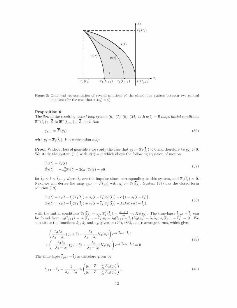
Figure 3: Graphical representation of several solutions of the closed-loop system between two controlimpulses (for the case that x1(tj) < 0).

Proposition 6

The flow of the resulting closed-loop system (6), (7), (9), (34) with µ(t) = µ maps initial conditions

x−(tj) ∈ E to x

−(tj+1) ∈ E , such that

yj+1 = F (yj), (36)

with yj = x1(tj), is a contraction map.

Proof Without loss of generality we study the case that yj := x1(tj) < 0 and therefore k3(yj) > 0.We study the system (11) with µ(t) = µ which obeys the following equation of motion

x1(t) = x2(t)

x2(t) = −ω2nx1(t) − 2ζωnx2(t) − gµ

(37)

for tj < t < tj+1, where tj are the impulse times corresponding to this system, and x1(tj) < 0.Next we will derive the map yj+1 = F (yj) with yj := x1(tj). System (37) has the closed formsolution (19)

x1(t) = s1(t − tj)x1(tj) + s2(t − tj)x+2 (tj) − c

(1 − s1(t − tj)

),

x2(t) = s1(t − tj)x1(tj) + s2(t − tj)x+2 (tj) − λ1λ2c s2(t − tj),

(38)

with the initial conditions x1(tj) = yj , x+2 (tj) =

k3(yj)m =: K3(yj). The time-lapse tj+1 − tj can

be found from x2(tj+1) = s1(tj+1 − tj)yj + s2(tj+1 − tj)K3(yj) − λ1λ2c s2(tj+1 − tj) = 0. Wesubstitute the functions s1, s2 and s2, given in (20), (83), and rearrange terms, which gives

(λ1λ2

λ2 − λ1(yj + c) − λ1

λ2 − λ1K3(yj)

)

eλ1(tj+1−tj)

+

(

− λ1λ2

λ2 − λ1(yj + c) +

λ2

λ2 − λ1K3(yj)

)

eλ2(tj+1−tj) = 0.

(39)

The time-lapse tj+1 − tj is therefore given by

tj+1 − tj =1

λ2 − λ1ln

(

yj + c − 1λ2

K3(yj)

yj + c − 1λ1

K3(yj)

)

, (40)

12

which is bounded because yj ≥ −c, i.e. tj+1 − tj ≤ 1λ2−λ1

ln (λ1/λ2). The return value yj+1 of the

map equals F (yj) = x1(tj+1), which yields

F (yj) = s1(tj+1 − tj)(yj + c) + s2(tj+1 − tj)K3(yj) − c

= a2

(

yj + c − K3(yj)

λ2

)

eλ1(tj+1−tj) + a1

(

yj + c − K3(yj)

λ1

)

eλ2(tj+1−tj) − c(41)

with

a1 := − λ1

λ2 − λ1, a2 :=

λ2

λ2 − λ1. (42)

Substitution of (40) in (41) gives

F (yj) =a2

(

yj + c − K3(yj)

λ2

)(

yj + c − 1λ2

K3(yj)

yj + c − 1λ1

K3(yj)

)−a1

+

a1

(

yj + c − K3(yj)

λ1

)(

yj + c − 1λ2

K3(yj)

yj + c − 1λ1

K3(yj)

)a2(43)

which can be simplified using a1 + a2 = 1 to

F (yj) =

(

c + yj −K3(yj)

λ2

)a2(

c + yj −K3(yj)

λ1

)a1

− c

= c

[(

1 +yj

c− K3(yj)

cλ2

)a2(

1 +yj

c− K3(yj)

cλ1

)a1

− 1

]

.

(44)

Clearly, F (y) has a fixed point at y∗ = F (y∗) if K3(y∗) = 0. The map F has therefore a unique

fixed point at y = 0.In order to study the contraction properties of this map, we now would have to evaluate the

derivative F′(y), but a direct evaluation of this derivative is obstructed by the fact that K ′

3(0)does not exist (note that k′

3(0) does not exist due to (31), (32)). Here, we use the Taylor expansion

(1+x)a ≈ 1+ax+ a(a−1)2 x2 on each of the terms in the brackets in the expression (44) and retain

terms of O(y). Note that K3(y) = O(√

y) and K3(y)2 = O(y), see (33). For small values of y, we

can therefore approximate F with

F (y) = c

[(

1 + a2y

c− a2

K3(y)

λ2c+

a2(a2 − 1)

2

K23 (y)

λ22c

2

)

·

(

1 + a1y

c− a1

K3(y)

λ1c+

a1(a1 − 1)

2

K23 (y)

λ21c

2

)

− 1

]

+ O(y32 )

= c

[

(a1 + a2)y

c−(

a2

λ2+

a1

λ1

)K3(y)

c+

(a1a2

λ1λ2+

a2(a2 − 1)

2λ22

+a1(a1 − 1)

2λ21

)K2

3 (y)

c2

]

+ O(y32 ).

(45)

The following coefficients appear in (45) a1 + a2 = 1, a2

λ2+ a1

λ1= 0, and

a1a2

λ1λ2+

a2(a2 − 1)

2λ22

+a1(a1 − 1)

2λ21

=a1a2

λ1λ2− a2a1

2λ22

− a1a2

2λ21

=1

2λ1λ2=

1

2

1

ω2n

. (46)

Hence, the map F is approximated to leading order by

F (y) = y +1

2

1

ω2n

K23(y)

c+ O(y

32 ) (47)

13

and k3(y) ≈ k3approx(y) = − sign(y)√

2cω2nm2|y| for small values of |y|, see (33). The slope of

the map at the fixed point y = 0 therefore yields F′(0) = 1 − c/c = 1 − µ/µ, which fulfills the

condition 0 ≤ F′(0) < 1 because 0 < µ ≤ µ. Note that if another control law would have been

chosen for which K ′3(0) is bounded, then it would hold that F

′(0) = 1. For y 6= 0, the slope F

′(y)

is much easier to obtain as K ′3(y) is bounded for y 6= 0. For y < 0 we have

F′(y) = a2

(

1 +y

c− K3(y)

cλ2

)−a1(

1 +y

c− K3(y)

cλ1

)a1(

1 − K ′3(y)

λ2

)

+ a1

(

1 +y

c− K3(y)

cλ1

)−a2(

1 +y

c− K3(y)

cλ2

)a2(

1 − K ′3(y)

λ1

)

.

(48)

We introduce the following abbreviations:

L1 = 1 +y

c− K3(y)

cλ1, L2 = 1 +

y

c− K3(y)

cλ2, Z1 =

(

1 − K ′3(y)

λ1

)

, (49)

L1 = 1 +y

c− K3(y)

cλ1, L2 = 1 +

y

c− K3(y)

cλ2, Z2 =

(

1 − K ′3(y)

λ2

)

. (50)

Using these abbreviations, together with a1 + a2 = 1, we write the slope F′(y) for y < 0 as

F′(y) = a2L

−a1

2 La1

1 Z2 + a1L−a2

1 La2

2 Z1 = a2

(L2

L1

)a2−1

Z2 + a1

(L2

L1

)a2

Z1

=

(L2

L1

)a2 (

a2

(L1

L2

)

Z2 + a1Z1

)

.

(51)

We now use the fact that a2

λ2+ a1

λ1= 0 and therefore a2Z2 + a1Z1 = 1 to arrive at

F′(y) =

(L2

L1

)a2 (

1 + a2Z2

(L1

L2

− 1

))

. (52)

It holds that F (y) = F ′(y) = 0 for µ(t) = µ, so 0 = 1 + a2Z2 (L2/L1 − 1). Substitution of thelatter gives

F′(y) =

(L2

L1

)a2

1 −L1

L2

− 1

L1

L2

− 1

=

(L2

L1

)a2 (

1 − L1 − L2

L1 − L2

L2

L2

)

=

(L2

L1

)a2 (

1 −µ

µ

L2

L2

)

. (53)

Because a2 > 0, L2

L1

< 1 andL

2

L2

> 1 for y < 0, it holds that the map F has its largest slope for

y = 0, i.e. F′(y) ≤ 1 − µ/µ. The symmetry of the problem implies that |F (y)| ≤ (1 − µ/µ)|y| for

all y. The map F is therefore a contraction mapping, i.e.

|yj+1| ≤(

1 −µ

µ

)

|yj |, (54)

since 0 ≤ 1 − µ

µ < 1 due to the fact that 0 < µ ≤ µ by the adoption of Assumption 1. Hence, the

sequence yj = x1(tj) converges to zero as j → ∞.

We now return to the problem that a solution x+(tj) is confined to the set χ, but (if no

additional assumptions are made) might approach the end of the stick set E(t) asymptotically andmight therefore not return to x

−(tj+1) ∈ E in a finite time tj+1 < ∞. To avoid such undesirablebehaviour, we adopt the following assumption.

Assumption 3

We assume that µ < 2µ.

14

Under this assumption it holds that the previously defined map F in (36) satisfies F (−c) ≥(1 − µ/µ

)· (−c) > −c. This assumption restricts the Γµ border of χ to end in E . This fact will,

in turn, be used to show that solutions of the resulting closed-loop system with time-varying µ(t)return in finite time to E .

Proposition 7

A solution of the resulting closed-loop system (6), (7), (9), (34), satisfying Assumptions 1 and 3,

which starts in E at t = t1 returns to E in a finite time interval t2 − t1.

Proof The proof is given in Appendix B.

Next, we consider the impulse times tj with j > 2 and x−(t2) ∈ E . We prove that if x

−(t2) ∈E− then it holds that x

−(tj) ∈ E− for all j > 2. Similar reasoning holds for x−(t2) ∈ E+ due to

the symmetry properties of the system.

Proposition 8

Solutions of the resulting closed-loop system (6), (7), (9), (34) with a friction coefficient µ(x1, x2, t),

satisfying Assumptions 1 and 3, which start in E− at t = tj return to E− in a finite time tj+1 − tjwith the lower and upper bounds tj+1 ≤ tj+1 ≤ tj+1 given by

tj+1 − tj =1

λ2 − λ1ln

(−λ1λ2 (x1(tj) + c) + λ1x+2 (tj)

−λ1λ2 (x1(tj) + c) + λ2x+2 (tj)

)

, (55)

tj+1 − tj =1

λ2 − λ1ln

(−λ1λ2 (x1(tj) + c) + λ1x+2 (tj)

−λ1λ2 (x1(tj) + c) + λ2x+2 (tj)

)

, (56)

with x1(tj+1) ≤ x1(tj+1) ≤ x1(tj+1) = 0.

Proof The proof is given in Appendix B.

We conclude that if x−(tj) ∈ E , then the solution x(t) ∈ χ for t ∈ (tj , tj+1) and that this solution

will hit the line x2 = 0 in finite time-lapse tj+1 − tj with lower and upper bound given by (55)and (56), respectively. Note that, due to Proposition 2, we have that x2(t

+j ) = mk3(x1(tj)) is

bounded and, consequently, both tj+1 and tj+1 are upper bounded, which also follows from (92).In other words, after an impulsive control action a finite time interval of smooth flow follows beforethe next control impulse is applied.

Next, we exploit Proposition 8, which states that the position errors yj = x1(tj) at the impulsetimes tj converge to zero faster for system (11) with time-varying µ(t) than for system (11) withµ(t) = µ. Note that Proposition 8 only holds for initial conditions in E .

Proposition 9

The flow of the resulting closed-loop system (6), (7), (9), (34) with a friction coefficient µ(x1, x2, t),satisfying Assumptions 1 and 3, maps initial conditions x

−(tj) ∈ E to x−(tj+1) ∈ E , such that

yj+1 = F (yj), (57)

with yj = x1(tj), is a contraction map.

Proof Proposition 8 proves that if −c ≤ yj ≤ 0, then it holds that F (yj) ≤ F (yj) ≤ 0. Proposi-tion 6 proves that F is a contraction map, hence the map F is also a contraction map within E .

Proposition 9 proves that the sequence yj = x1(tj) converges to zero (i.e. the positioning error atthe impulse times converges to zero). Next, we show that the position error converges to zero infinite time.

15

Proposition 10

A solution of the resulting closed-loop system (6), (7), (9), (34) with a friction coefficient µ(x1, x2, t),satisfying Assumptions 1 and 3, and initial condition x

−(t2) ∈ E reaches the origin in a finite time

t∞ − t2 ≤√

2|y2|gµ

1

1 −(

1 − µ

µ

) 12

, (58)

with y2 = x1(t2) and x(t∞) = 0.

Proof The time difference between two consecutive impacts is bounded from above by (92) with

x1(tj) = yj , i.e. tj+1 − tj ≤√

2|yj |cω2

n=√

2|yj |gµ . The total time to arrive at the origin amounts to

T := t∞ − t2 =

∞∑

j=2

tj+1 − tj ≤√

2

gµ

∞∑

j=2

√

|yj |. (59)

Recursive usage of the contraction property in (54) yields

|yj| ≤(

1 −µ

µ

)j−2

|y2|. (60)

Inequality (60) in combination with (59) gives the upper bound

T ≤√

2|y2|gµ

∞∑

j=2

(

1 −µ

µ

) 12j−1

=

√

2|y2|gµ

∞∑

j=0

(

1 −µ

µ

) 12j

. (61)

Using the convergent geometric series

∞∑

j=0

x1/2j =

∞∑

j=0

(x1/2)j = 1/(1 − x1/2) |x| < 1, (62)

we can give the conservative estimate

T ≤√

2|y2|gµ

∞∑

j=0

(

1 −µ

µ

) 12j

=

√

2|y2|gµ

1

1 −(

1 − µ

µ

) 12

, (63)

which gives an upper bound for the finite attraction time. Since |y2| ≤ c is bounded and Assump-tion 1 is satisfied, we can conclude that the attraction is symptotic.

Proposition 11

Consider the resulting closed-loop system (6), (7), (9), (34) satisfying Assumptions 1, 2 and 3.The solutions of the resulting closed-loop system are bounded and converge to x = 0 in a finitetime.

Proof Boundedness is proven in Proposition 3. Assumption 2 assures that a solutions withan arbitrary initial condition x(t0) ∈ R

2 reaches E is a finite time t1. Under Assumption 3,Proposition 7 proves that any solution of the resulting closed-loop system which starts in E att = t1 returns to E in a finite time t2. Propositions 9 and 10 prove that a solution which starts inx−(t2) ∈ E reaches the origin in a finite time.

Finally, we will show that the origin of the resulting closed-loop system is globally uniformlysymptotically stable.

16

Theorem 1

Consider the resulting closed loop system (6), (7), (9), (34) satisfying Assumptions 1, 2 and 3.The origin of the resulting closed-loop system is globally uniformly symptotically stable.

Proof Consider the candidate Lyapunov function V (x) = 12mx2

2 + 12k1x

21 and with some abuse of

notation V (t) = V (x+(t)), i.e. the function V (t) is right-continuous. Let us denote the value of the

Lyapunov function V (tj) at impulse time-instants tj by Vj := V (tj) = 12m(x+

2 (tj))2

+ 12k1x

21(tj).

Using the notation yj = x1(tj) and the fact that x+2 (tj) = k3(x1(tj))/m = K3(yj), the increment

Vj+1 − Vj satisfies:

Vj+1 − Vj =1

2k1

(y2

j+1 − y2j

)+

1

2m(K2

3 (yj+1) − K23(yj)

). (64)

Propositions 6, 7, and 9 prove the contraction properties (54): |yj+1| ≤(1 − µ/µ

)|yj|, for j ≥ 1.

Moreover, the impulsive control law K3(y) is monotonically decreasing, see e.g. (30) in Sec-tion 3.2.1, i.e. (K3(y2) − K3(y1)) (y2 − y1) < 0 ∀y1, y2. It therefore holds that |K3(yj+1)| <|K3(yj)| as well as

K23(yj+1) − K2

3 (yj) < 0. (65)

Using (65) and Assumption 1 in (64) yields

Vj+1 − Vj <1

2k1

(y2

j+1 − y2j

)<

1

2k1

((

1 −µ

µ

)2

− 1

)

y2j < 0 (66)

for yj 6= 0. In other words, the Lyapunov function strictly decreases along the impulse timeinstants tj . Let us now investigate the evolution of the Lyapunov function in between the impulse

times (i.e. for t ∈ (tj , tj+1)): V = −k2x22−mgµ(x1, x2, t) |x2| ≤ −k2x

22−mgµ |x2|. Since x2(t) 6= 0

for all t ∈ (tj , tj+1) we have that V (t) < Vj , for t ∈ (tj , tj+1) , j ≥ 1. Moreover, it holds that

V (t) ≤ 0 for t ∈ [t0, t1). Let us define V 0 := max(V0, V1). We can construct a function βV (V 0, t)as follows:

βV (V 0, t − t0) =

V 0 t0 ≤ t < t2V2−V 0

t3−t2(t − t2) + V 0 t2 ≤ t < t3

Vj−Vj−1

tj+1−tj(t − tj) + Vj−1 tj ≤ t < tj+1, j > 2

0 t ≥ t∞,

(67)

such that

V (t) ≤ βV (V 0, t − t0), t ≥ t0, (68)

where we used that V (t∞) = 0 because x(t∞) = 0, see Proposition 10. Clearly, βV (V 0, t − t0)is a continuous function of V 0 and a continuous function of t because limj→∞ Vj = 0. For fixedt − t0, the mapping βV (V 0, t − t0) is upper bounded by a class K∞ function with respect to V 0.Moreover, since Vj , j ≥ 1, is a strictly decreasing series tending to zero, see (66), we have that, forfixed V 0, the mapping βV (V 0, t − t0) is decreasing with respect to t − t0 and βV (V 0, t − t0) = 0for t ≥ t∞ (where t∞ is bounded, see Proposition 11). Hence, βV is upper bounded by a class KLfunction βV (V 0, t − t0) := βV (V 0, t − t0) + εV 0e

(t0−t), with ε > 0. Hence, we can conclude thatV (t) is upper bounded by a class KL function according to

V (t) ≤ βV (V 0, t − t0), t ≥ t0. (69)

Since it holds that α1(|x|) ≤ V (x) ≤ α2(|x|), with α1(|x|) := min(k1

2 , m2 )|x|2 and α2(|x|) :=

max(k1

2 , m2 )|x|2, we can conclude from (69) that

|x(t)| ≤ α−11 βV (V 0, t − t0), t ≥ t0. (70)

17

Next, let us use that V 0 = max(V0, V1) ≤ max(α2(|x(t0)|), α2(|x+(t1)|)) = α2(max(|x(t0)|, |x+(t1)|)),since α2(·) is a K∞-function. Combining the latter fact with (70) yields

|x(t)| ≤ α−11 βV (α2(max(|x(t0)|, |x+(t1)|)), t − t0), t ≥ t0. (71)

Consider a class K∞-function γ(·) such that γ(|x−(t1)|) ≥ (x−1 (t1))

2 + K23 (x−

1 (t1)) ∀x−(t1) ∈E , which indeed exists and only depends on |x−(t1)| because of the symmetry properties andboundedness of K3 and the fact that |x−(t1)| = |x−

1 (t1)|. Consequently, |x+(t1)| = (x−1 (t1))

2 +K2

3 (x−1 (t1)) ≤ γ(|x−(t1)|) and in turn it holds that V (x+(t1)) ≤ α2(γ(|x−(t1)|)). Combining

the latter fact with the implication V (x−(t1)) ≤ V (x(t0)) ⇒ α−11 α2(|x(t0)|) ≥ |x−(t1)|, gives

V (x+(t1)) ≤ α2 γ α−11 α2(|x(t0)|). Consequently, we can conclude that |x+(t1)| ≤ α−1

1 α2 γ α−1

1 α2(|x(t0)|). Combining the latter fact with (71) yields

|x(t)| ≤ α−11 βV (α2(max(|x(t0)|, α−1

1 α2 γ α−11 α2(|x(t0)|))), t − t0), t ≥ t0. (72)

If we define α2(|x(t0)|) := α2(max(|x(t0)|, α−11 α2 γ α−1

1 α2(|x(t0)|))), this inequality can bewritten as

|x(t)| ≤ α−11 βV (α2(|x(t0)|), t − t0) =: βx(|x(t0)|, t − t0), t ≥ t0, (73)

where βx(s, t) is a class KL function, since α2 is a class K∞-function and βV (s, t) is a classKL function. In other words the equilibrium point is globally uniformly asymptotically stable.Moreover, since all solutions of the system converge to the origin in finite time, see Proposition 11,the origin is globally uniformly symptotically stable. This completes the proof.

5 Illustrative Example

In this section, we illustrate the effectiveness of the impulsive control strategy, developed in thispaper, by means of an example. Hereto, we consider a motion system as in Figure 1 with dynamicsdescribed by (6), where the inertia is taken to be m = 1 and the gravitational acceleration g = 10.Moreover, the friction coefficient in (6) is of the form µ(x1, x2, t) = (µ1 − µ2)/(1 + 0.5|x2|) + µ2 +µ3 sin(Ωt), where µ1 = 0.4, µ2 = 0.3, µ3 = 0.05 and Ω = 4. In this friction law one can recognisea velocity-dependency with a pronounced Stribeck effect and an explicit time-dependency. Notethat this friction law satisfies Assumption 1 with µ = 0.25 and µ = 0.45, which indicates asignificant possible variation on the friction coefficient and which also implies the satisfaction ofAssumption 3. The possible variation of the friction coefficient is also illustrated by the dashedlines in Figure 4. Next, we employ the switching impulsive controller design proposed in Section 3and described by (7), (9), (34). Herein, the control parameters are designed as k1 = 1, k21 = 0.5,k22 = 3, implying that 0 < k21

2√

k1m= 0.25 < 1 and k22

2√

k1m= 1.5 > 1 as proposed in Section 3.3,

and the impulsive control design (9) is designed as depicted in Figure 5, where k3(y) = K3(y)since m = 1.

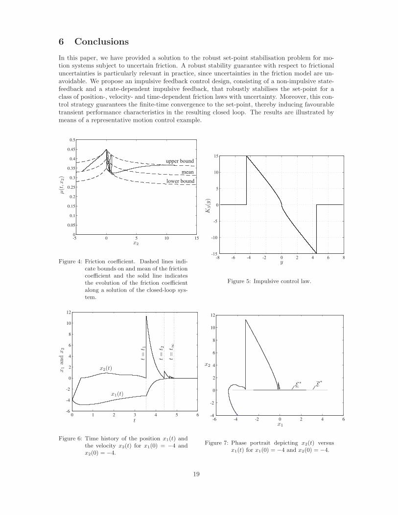
Figures 6 and 7 depict a simulated response of the closed-loop system for an initial conditionx1(0) = −4 and x2(0) = −4. Figure 8 shows the corresponding time evolution of the frictioncoefficient along this solution of the closed-loop system (a different perspective on the variationof the friction coefficient along the same solution of the closed-loop system is represented by thesolid line in Figure 4). Figures 6 clearly shows that the response indeed converges to the originin finite time, while the jumps in the velocity induced by the impulsive control action are clearlyvisible. This figure also displays the time instants t1 = 3.55 and t2 = 4.40 at which the responsehits, for the first time, the sets E (maximal stick set) and E (minimal stick set), respectively (seealso Figure 7). Moreover, the response converges to the origin in the finite time t∞ = 4.8707.The upper bound on t∞ that can be computed using Proposition 10 is t∞ = 5.5162. This upperbound on t∞ is not overly conservative and can be considered to be a realistic bound on the timein which convergence to the setpoint is achieved.

We care to stress that the impulsive control design by no means exploits knowledge on theparticular friction law used in this example and indeed guarantees robust stabilisation for anyposition-, velocity- and time-dependent friction coefficient satisfying the same bounds.

18

6 Conclusions

In this paper, we have provided a solution to the robust set-point stabilisation problem for mo-tion systems subject to uncertain friction. A robust stability guarantee with respect to frictionaluncertainties is particularly relevant in practice, since uncertainties in the friction model are un-avoidable. We propose an impulsive feedback control design, consisting of a non-impulsive state-feedback and a state-dependent impulsive feedback, that robustly stabilises the set-point for aclass of position-, velocity- and time-dependent friction laws with uncertainty. Moreover, this con-trol strategy guarantees the finite-time convergence to the set-point, thereby inducing favourabletransient performance characteristics in the resulting closed loop. The results are illustrated bymeans of a representative motion control example.

Figure 4: Friction coefficient. Dashed lines indi-cate bounds on and mean of the frictioncoefficient and the solid line indicatesthe evolution of the friction coefficientalong a solution of the closed-loop sys-tem.

-8 -6 -4 -2 0 2 4 6 8-15

-10

-5

0

5

10

15

Figure 5: Impulsive control law.

Figure 6: Time history of the position x1(t) andthe velocity x2(t) for x1(0) = −4 andx2(0) = −4.

Figure 7: Phase portrait depicting x2(t) versusx1(t) for x1(0) = −4 and x2(0) = −4.

19

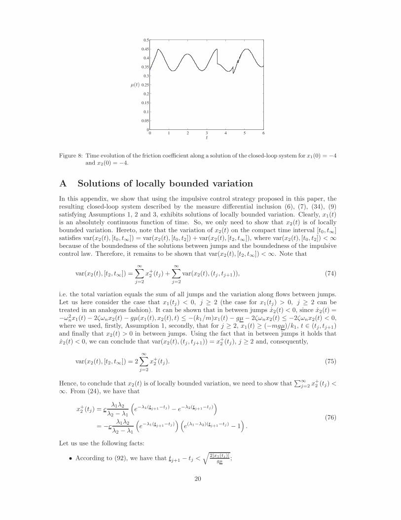
Figure 8: Time evolution of the friction coefficient along a solution of the closed-loop system for x1(0) = −4and x2(0) = −4.

A Solutions of locally bounded variation

In this appendix, we show that using the impulsive control strategy proposed in this paper, theresulting closed-loop system described by the measure differential inclusion (6), (7), (34), (9)satisfying Assumptions 1, 2 and 3, exhibits solutions of locally bounded variation. Clearly, x1(t)is an absolutely continuous function of time. So, we only need to show that x2(t) is of locallybounded variation. Hereto, note that the variation of x2(t) on the compact time interval [t0, t∞]satisfies var(x2(t), [t0, t∞]) = var(x2(t), [t0, t2]) + var(x2(t), [t2, t∞]), where var(x2(t), [t0, t2]) < ∞because of the boundedness of the solutions between jumps and the boundedness of the impulsivecontrol law. Therefore, it remains to be shown that var(x2(t), [t2, t∞]) < ∞. Note that

var(x2(t), [t2, t∞]) =

∞∑

j=2

x+2 (tj) +

∞∑

j=2

var(x2(t), (tj , tj+1)), (74)

i.e. the total variation equals the sum of all jumps and the variation along flows between jumps.Let us here consider the case that x1(tj) < 0, j ≥ 2 (the case for x1(tj) > 0, j ≥ 2 can betreated in an analogous fashion). It can be shown that in between jumps x2(t) < 0, since x2(t) =−ω2

nx1(t) − 2ζωnx2(t) − gµ(x1(t), x2(t), t) ≤ −(k1/m)x1(t) − gµ − 2ζωnx2(t) ≤ −2ζωnx2(t) < 0,where we used, firstly, Assumption 1, secondly, that for j ≥ 2, x1(t) ≥ (−mgµ)/k1, t ∈ (tj , tj+1)and finally that x2(t) > 0 in between jumps. Using the fact that in between jumps it holds thatx2(t) < 0, we can conclude that var(x2(t), (tj , tj+1)) = x+

2 (tj), j ≥ 2 and, consequently,

var(x2(t), [t2, t∞]) = 2

∞∑

j=2

x+2 (tj). (75)

Hence, to conclude that x2(t) is of locally bounded variation, we need to show that∑∞

j=2 x+2 (tj) <

∞. From (24), we have that

x+2 (tj) = c

λ1λ2

λ2 − λ1

(

e−λ1(tj+1−tj) − e−λ2(tj+1

−tj))

= −cλ1λ2

λ2 − λ1

(

e−λ1(tj+1−tj)

)(

e(λ1−λ2)(tj+1−tj) − 1

)

.

(76)

Let us use the following facts:

• According to (92), we have that tj+1 − tj <√

2|x1(tj)|gµ ;

20

• |x1(tj)| ≤ mgµ

k1,

to conclude that tj+1 − tj <√

2ωn

. Using the latter fact, the following statements are valid:

• e−λ1(tj+1−tj) ≤ e−λ1

√2

ωn for (tj+1 − tj) ≤√

2ωn

;

• e(λ1−λ2)(tj+1−tj) − 1 ≤ (λ1 − λ2)e

(λ1−λ2)√

2

ωn (tj+1 − tj), for (tj+1 − tj) ≤√

2ωn

.

Using the latter facts in (76) gives

x+2 (tj) ≤ −c

λ1λ2

λ2 − λ1

(

e−λ1

√2

ωn

)(

(λ1 − λ2)e(λ1−λ2)

√2

ωn

) (tj+1 − tj

)

≤ cλ1λ2e−λ2

√2

ωn

(tj+1 − tj

)=: M

(tj+1 − tj

)(77)

with M > 0 bounded. Hence, we can conclude that

∞∑

j=2

x+2 (tj) ≤ M

∞∑

j=2

(tj+1 − tj

)≤ M

√

2|x1(t2)|gµ

1

1 −(

1 − µ

µ

) 12

, (78)

where we used (63). Subsequently using the fact that |x1(t2)| ≤ mgµ

k1and Assumption 3 yields

∞∑

j=2

x+2 (tj) ≤

2M

(√

2 − 1)ωn

< ∞. (79)

Hence, the combination of (75) and (79) shows that var(x2(t), [t2, t∞]) < ∞, which also impliesthat x2(t) is of locally bounded variation. Hence, this validates the formulation of the resultingclosed-loop system in terms of a measure differential inclusion.

B Proofs

B.1 Proof of Proposition 1

By exploiting the Laplace transforms Xi(s) = L(xi(t)), i = 1, 2, F (s) = L(f(t)), (15) can betransformed to sX1(s) − x10 = X2(s), sX2(s) − x20 = −ω2

nX1(s) − 2ζωnX2(s) + F (s), and weobtain that it holds that X1(s) = S1(s)x10 + S2(s)x20 + S2(s)F (s), where the S1(s) and S2(s) arethe transfer functions of the initial conditions given by

S1(s) =s + 2ζωn

s2 + 2ζωns + ω2n

=λ2

λ2 − λ1

1

s − λ1− λ1

λ2 − λ1

1

s − λ2, (80)

S2(s) =1

s2 + 2ζωns + ω2n

= − 1

λ2 − λ1

1

s − λ1+

1

λ2 − λ1

1

s − λ2. (81)

We take the inverse Laplace transform of S1(s) and S2(s) to obtain the expressions for s1(t), s2(t)as in (20), for which it holds that s1(0) = 1, s2(0) = 0 and the following inequalities hold

s1(t) > 0 ∀ t > − 1λ2−λ1

ln(

λ1

λ2

)

,

s2(t) > 0 ∀ t > 0.(82)

Differentiation of (20) with respect to time gives

s1(t) = −λ1λ2 s2(t),

s2(t) =1

λ2 − λ1

(−λ1e

λ1t + λ2eλ2t)

= s1(t) + (λ1 + λ2) s2(t),(83)

21

and it therefore holds that s2(t) > 0 for t < 1λ2−λ1

ln λ1

λ2from which we conclude, using (82), that

s2(t) > 0 ⇐⇒ s1(−t) > 0. (84)

The general solution of (15), with the initial condition (16) and on a non-impulsive time-intervalfor which x2(t) 6= 0 does not change sign, can therefore be written as

x1(t) = s1(t − t0)x10 + s2(t − t0)x20 +

∫ t

t0

s2(t − τ)f(τ) dτ,

x2(t) = s1(t − t0)x10 + s2(t − t0)x20 +

∫ t

t0

s2(t − τ)f(τ) dτ.

(85)

We now decompose the input f(t) in a constant input fconst and a time-varying input fvar(t), i.e.

f(t) = −gµconst sign(x2)︸ ︷︷ ︸

fconst

−g (µ(t) − µconst) sign(x2)︸ ︷︷ ︸

fvar(t)

(86)

for some µconst > 0. The convolution integrals in (85) of the constant input yield

∫ t

t0

s2(t − τ)fconst dτ =

[fconst

λ1λ2s1(t − τ)

]t

t0

=fconst

λ1λ2(1 − s1(t − t0)) , (87)

∫ t

t0

s2(t − τ)fconst dτ = [−fconst s2(t − τ)]tt0

= fconst s2(t − t0). (88)

If x2 > 0 and µconst = µ, then it holds that fvar(t) ≤ 0 for all t and, using the inequalities (82), (84),we arrive at the following inequalities for the convolution integrals of the time-varying input f(τ)in (85):

∫ t

t0

s2(t − τ)fvar(τ) dτ ≤ 0 t − t0 ≥ 0,

∫ t

t0

s2(t − τ)fvar(τ) dτ ≤ 0 t − t0 ≤ 1

λ2 − λ1ln

λ1

λ2.

(89)

Similarly, if x2 > 0 and µconst = µ, then it holds that fvar(t) ≥ 0 and the inequalities forthe convolution integrals change sign. Let (x1(t), x2(t)) denote the solution of the initial valueproblem (15), (16) for µ(t) = µ and (x1(t), x2(t)) for µ(t) = µ. The latter two solutions forconstant µ and positive velocity x2 > 0 can be expressed in closed form as in (18) and (19).Similar expressions can obviously be derived for the case that x2 < 0. The inequalities on thetime-varying input in (89) imply that, for a certain time-interval, the solution (x1(t), x2(t)) islower and upper bounded by the solutions (x1(t), x2(t)) and (x1(t), x2(t)) according to (21).

B.2 Proof of Proposition 2

We first investigate the slope of f(t) given by

f′(t) = cλ1λ2 s2(tj − t) = −c

λ1λ2

λ2 − λ1

(

eλ1(tj−t) − eλ2(tj−t))

. (90)

It holds that f′(tj) = 0 and f

′(tj+1) = −x+2 (tj). Further differentiation gives

f′′(t) = −cλ1λ2 s2(tj − t) = −c

λ1λ2

λ2 − λ1

(

−λ1eλ1(tj−t) + λ2e

λ2(tj−t))

= −λ2f′(t) − cλ1λ2e

λ1(tj−t).

(91)

22

The slope f′(t) is strictly negative on the open domain t > tj . In addition, it can easily be

checked that also f′′(t) < −cω2

n < 0 on the domain t > tj . We can therefore conclude that, for ζ >1, the algebraic equation f(tj+1) = 0 has a unique solution. Moreover, on the domain t > tj , the

function f is bounded from above by a concave parabola, i.e. f(tj+1) < − 12 cω2

n(tj+1− tj)2−x1(tj),

and the end time therefore has the upper bound

tj+1 − tj <

√

2|x1(tj)|cω2

n

=

√

2|x1(tj)|gµ

. (92)

The value of x+2 (tj) is determined by the evaluation of x2(t), given by (24) at t = tj using the

previously calculated value of tj+1. Since tj+1 is bounded, due to the fact that x1 is bounded for

all (x1, x2) ∈ E , also x+2 (tj) is bounded.

Subsequently, the impulsive control action k3(x1(tj)) can be computed from (27). Hence,k3(x1) is uniquely defined and bounded for all (x1, x2) ∈ E and the proof is complete.

B.3 Proof of Proposition 3

Consider the energy function V (x) = 12mx2

2 + 12k1x

21. Define the set Ω = x ∈ R

2 | V (x) >

12k1

(mgµk1

)2

. By definition of the impulsive part of the control law (9) no impulsive control

action will occur for x ∈ Ω because Ω ∩ E = ∅. Hence, using (11), the time-derivative of Valong solutions of the closed-loop system can be evaluated with V = −k2x

22−mgµ(x1, x2, t) |x2| ≤

−k2x22 − mgµ |x2|, for x ∈ Ω. The parameter k2(t) switches from k21 > 0, for t0 ≤ t < t1, to a

larger value k22 > 0, for t ≥ t1. It holds that V ≤ 0 for x ∈ Ω, implying that solutions can notgrow unbounded along flows. The switching of k2 such that ζ > 1 when the impulsive controlleris switched on guarantees the satisfaction of the conditions of Proposition 2 and therewith impliesthat U = k3(x1) is defined and bounded for all x ∈ E , whereas U = 0 for x /∈ E . The impulsivecontrol force U is therefore bounded and leads to a bounded jump in x2. Hence the boundednessof solutions in forward time is guaranteed.

B.4 Proof of Proposition 7

Without loss of generality we consider the case x1(t1) < 0. Under Assumption 3 and (54), it holdsthat F (−c) ≥

(1 − µ/µ

)· (−c) > −c and therefore x1(t2) ≥ −c + c > −c. Solutions can therefore

only escape the set χ, see Figure 3, through the ”inner” part −c < x1 ≤ 0 of E−. The stick set E−

is therefore reached in a finite time, because the edges of the stick set E(t) ⊇ E can not be reached(see [5,8]). We can estimate the time lapse t2 − t1 by evaluation of the condition x−

2 (t2) = 0 usingthe general solution as in (85) with t0 = t2 as reference time x+

2 (t1) = −λ1λ2s2(t1 − t2)(x1(t2) +

c)+∫ t1

t2s2(t1− τ)fvar(τ) dτ with fvar = −g(µ(t)−µ) ≤ 0. The inequalities s2(t) < 0, s2(t) > 1 for

t < 0, together with t2 > t1, give x+2 (t1) > −λ1λ2s2(t1−t2)(x1(t2)+c) > −λ1λ2s2(t1−t2)(−c+2c),

where we used that x1(t2) ≥ −c + c and, together with Assumption 3 and x+2 (t1) = K3(x1(t1)), it

therefore holds that

s2(t1 − t2) > − K3(x1(t1))

(2c − c)λ1λ2. (93)

Clearly, the time lapse

t2 − t1 < −s−12

(

− K3(x1(t1))

(2c− c)λ1λ2

)

(94)

is finite if Assumption 3 holds. The function s2(t) is strictly increasing for t < 0 as s2(t) > 1 andit therefore holds that s2(t) < t for t < 0, and correspondingly s−1

2 (x) > x for x < 0. The timelapse t2 − t1 can therefore be bounded from above by

t2 − t1 <K3(x1(t1))

(2c − c)λ1λ2. (95)

23

B.5 Proof of Proposition 8

Using (24) for t = tj , x1(tj) = −c(1 − s1(tj − tj+1)

)and the inequality −c ≤ x1(tj), because

x−(tj) ∈ E−, we find that s1(tj − tj+1) ≥ 0 and, using (82), it therefore holds that tj+1 − tj ≤1

λ2−λ1ln λ1

λ2. Hence, (21) in Proposition 1 holds, implying that the solution x(t) is wedged between

x(t) and x(t), i.e. x1(t) ≤ x1(t) ≤ x1(t), x2(t) ≤ x2(t) ≤ x2(t), for those t ∈ (tj , tj+1) such that the

velocities x2(t), x2(t) and x2(t) are strictly positive. We therefore deduce that tj+1 ≤ tj+1 ≤ tj+1.

The time-instant tj+1 is a lower bound for tj+1 and can be found from x2(tj+1) = 0. By using thegeneral solution (19) and taking t0 = tj as reference-time we obtain the expression

x2(tj+1) = s1(tj+1 − tj)x1(tj) + s2(tj+1 − tj)x+2 (tj) − λ1λ2c s2(tj+1 − tj) = 0. (96)

We substitute the functions s1, s2 and s2 and rearrange terms, which gives

(λ1λ2

λ2 − λ1(x1(tj) + c) − λ1

λ2 − λ1x+

2 (tj)

)

eλ1(tj+1−tj)

+

(

− λ1λ2

λ2 − λ1(x1(tj) + c) +

λ2

λ2 − λ1x+

2 (tj)

)

eλ2(tj+1−tj) = 0.

(97)

Further rearranging terms an taking the natural logarithm yields the time-lapse

tj+1 − tj =1

λ2 − λ1ln

(−λ1λ2 (x1(tj) + c) + λ1x+2 (tj)

−λ1λ2 (x1(tj) + c) + λ2x+2 (tj)

)

, (98)

which is strictly positive for x+2 (tj) > 0, because −c ≤ x1(tj) ≤ 0. Similarly, we obtain the

time-lapse

tj+1 − tj =1

λ2 − λ1ln

(−λ1λ2 (x1(tj) + c) + λ1x+2 (tj)

−λ1λ2 (x1(tj) + c) + λ2x+2 (tj)

)

, (99)

which gives the upper bound tj+1 for tj+1. Clearly, the upper bound (92) for tj+1 is also analternative upper bound for tj+1.

References

[1] Acary, V., and Brogliato, B. Numerical Methods for Nonsmooth Dynamical Systems.Applications in Mechanics and Electronics., vol. 35 of Lecture Notes in Applied and Compu-tational Mechanics. Springer Verlag, Berlin Heidelberg, 2008.

[2] Altpeter, F. Friction Modeling, Identification and Compensation. Ph.D. thesis, Dept.Genie Mech., Ecole Polytech. Fed. Lausanne, Switzerland, 1999.

[3] Armstrong-Helouvry, B., Dupont, P., and Canudas de Wit, C. A survey of models,analysis tools and compensation methods for the control of machines with friction. Automatica30, 7 (1994), 1083–1138.

[4] Armstrong-Helouvry, B. Control of Machines with Friction. Kluwer Academic Publish-ers, Boston, 1991.

[5] Cabot, A. Stabilization of oscillators subject to dry friction: finite time convergence versusexponential decay results. Transactions of the American Mathematical Society 360, 1 (2008),103–121.

[6] Canudas de Wit, C. Robust control for servo-mechanisms under inexact friction compen-sation. Automatica 29, 3 (1993), 757–761.

24

[7] Canudas de Wit, C., Olsson, H., Astrom, K., and Lischinsky, P. A new modelfor control of systems with friction. IEEE Transactions on Automatic Control 40, 3 (1995),419–425.

[8] Dıaz, J. I., and Millot, V. Coulomb friction and oscillation: stabilization in finite timefor a system of damped oscillators. In XVIII CEDYA: Congress on Differential Equationsand Applications / VIII CMA: Congress on Applied Mathematics, Tarragona (2003).

[9] Glocker, Ch. Set-Valued Force Laws, Dynamics of Non-Smooth Systems, vol. 1 of LectureNotes in Applied Mechanics. Springer-Verlag, Berlin, 2001.

[10] Hagglund, T. A friction compensator for pneumatic control valves. Journal of ProcessControl 12 (2002), 897–904.

[11] Hensen, R. H. A., Van de Molengraft, M. J. G., and Steinbuch, M. Friction inducedhunting limit cycles: A comparison between the LuGre and switch friction model. Automatica39 (2003), 2131–2137.

[12] Hojjat, Y., and Higuchi, T. Application of electromagnetic impulsive force to precisepositioning. International Journal of the Japan society for precision engineering 25, 11 (1991),39–44.

[13] Huang, W. Impulsive Manipulation. Ph.D. thesis, Carnegie Mellon University, U.S.A., 1997.

[14] Huang, W., and Mason, W. Mechanics, planning, and control for tapping. The Interna-tional Journal of Robotics Research 19, 10 (2000), 883–894.

[15] Iannelli, L., Johansson, K. H., Jonsson, U. T., and Vasca, F. Averaging of nons-mooth systems using dither. Automatica 42 (2006), 669–676.

[16] Ipri, S., and Asada, H. Tuned dither for friction suppression during force-guided roboticassembly. In Proceedings of the 1995 IEEE/RSJ International Conference on IntelligentRobots and Systems (1995), vol. 1, pp. 310–315.

[17] Johnson, C., and Lorenz, R. Experimental identification of friction and its compensationin precise position controlled mechanisms. IEEE Transactions on Industry Applications 28,6 (1992), 1392–1398.

[18] Kased, R., and Singh, T. High precision point-to-point maneuvering of an experimentalstructure subject to friction via adaptive impulsive control. In Proceedings of the 2006 IEEEInternational Conference on Control Applications, Germany (October 2006), pp. 3235–3240.

[19] Kim, J., and Singh, T. Desensitized control of vibratory systems with friction: linearprogramming approach. Optimal Control Applications and Methods 25 (2004), 165–180.

[20] Leine, R. I., and van de Wouw, N. Stability and Convergence of Mechanical Systemswith Unilateral Constraints, vol. 36 of Lecture Notes in Applied and Computational Mechanics.Springer Verlag, Berlin, 2008.

[21] Mallon, N. J., van de Wouw, N., Putra, D., and Nijmeijer, H. Friction compensationin a controlled one-link robot using a reduced-order observer. IEEE Trans. on Control SystemsTechnology 14, 2 (2006), 374–383.

[22] Moreau, J. J. Unilateral contact and dry friction in finite freedom dynamics. In Non-Smooth Mechanics and Applications, J. J. Moreau and P. D. Panagiotopoulos, Eds., vol. 302of CISM Courses and Lectures. Springer, Wien, 1988, pp. 1–82.

[23] Olsson, H., Astrom, K. J., Canudas de Wit, C., Gafvert, M., and Lischinsky, P.

Friction models and friction compensation. European Journal of Control 4, 3 (1998), 176–195.

25

[24] Orlov, Y. Santiesteban, R., and Aguilar, L. T. Impulsive control of a mechanicaloscillator with friction. In Proceedings of the 2009 IEEE American Control Conference, St.Louis, U.S.A. (June 2009), pp. 3494–3499.

[25] Panteley, E., Ortega, R., and Gafvert, M. An adaptive friction compensator forglobal tracking in robot manipulators. Systems & Control Letters 33 (1998), 307–313.

[26] Papadopoulos, E. G., and Chasparis, G. C. Analysis and model-based control of ser-vomechanisms with friction. In Proceedings of the 2002 IEEE/RSJ Int. Conf. on IntelligentRobots and Systems (Lausanne, Switzerland, 2002), pp. 2109–2114.

[27] Putra, D., van de Wouw, N., and Nijmeijer, H. Analysis of undercompensation andovercompensation of friction in 1DOF mechanical systems. Automatica 43, 8 (2007), 1387–1394.

[28] Siebenhaar, C. Precise adjustment method using stroke impulse and friction. PrecisionEngineering 28 (2004), 194–203.

[29] Southward, S., Radcliffe, C., and MacCluer, C. Robust nonlinear stick-slip frictioncompensation. ASME Journal of Dynamic Systems, Measurement, and Control 113 (1991),639–644.

[30] Taware, A., Tao, G., Pradhan, N., and Teolis, C. Friction compensation for a sand-wich dynamic system. Automatica 39, 3 (2003), 481–488.

[31] Thomsen, J. J. Using fast vibrations to quench friction-induced oscillations. Journal ofSound and Vibration 228, 5 (1999), 1079–1102.

[32] Wu, R., and Tung, P. Fast pointing control for systems with stick-slip friction. ASMEJournal of Dynamic Systems, Measurement and Control 126 (2004), 614–626.

[33] Yamagata, Y., and Higuchi, T. A micropositioning device for precision automatic assem-bly using impact force of piezoelectric elements. In Proceedings of the IEEE InternationalConference on Robotics and Automation (1995), pp. 666–671.

[34] Yang, S., and Tomizuka, M. Adaptive pulse width control for precise positioning under theinfluence of stiction and Coulomb friction. ASME Journal of Dynamic Systems, Measurementand Control 110, 3 (1988), 221–227.

26