Robust High Speed Autonomous Steering of an Off-Road Vehicle
134
Robust High Speed Autonomous Steering of an Off-Road Vehicle Michael Kapp Submitted in partial fulfilment of the requirements for the degree Master of Engineering (Mechanical Engineering) in the Faculty of Engineering, Built Environment and Information Technology (EBIT) at the University of Pretoria, Pretoria October 2014 © University of Pretoria
Transcript of Robust High Speed Autonomous Steering of an Off-Road Vehicle

Robust High Speed Autonomous Steeringof an Off-Road Vehicle
Michael Kapp
Submitted in partial fulfilment of the requirements for the degree
Master of Engineering(Mechanical Engineering)
in the Faculty of
Engineering Built Environment and Information Technology (EBIT)
at the
University of PretoriaPretoria
October 2014
copycopy UUnniivveerrssiittyy ooff PPrreettoorriiaa
II
Abstract
Title Robust High Speed Autonomous Steering of an Off-Road Vehicle
Author Michael Kapp
Study Leader Prof PS Els
Department Mechanical and Aeronautical Engineering University of Pretoria
Degree Masters in Engineering (Mechanical Engineering)
A ground vehicle is a dynamic system containing many non-linear components ranging from
the non-linear engine response to the tyre-road interface In pursuit of developing driver-
assist systems for accident avoidance as well as fully autonomous vehicles the application of
modern mechatronics systems to vehicles are widely investigated Extensive work has been
done in an attempt to model and control the lateral response of the vehicle system utilising a
wide variety of conventional control and intelligent systems theory The majority of driver
models are however intended for low speed applications where the vehicle dynamics are
fairly linear This study proposes the use of adaptive control strategies as robust driver
models capable of steering the vehicle without explicit knowledge of vehicle parameters A
Model Predictive Controller (MPC) self-tuning regulator and Linear Quadratic Self-Tuning
Regulator (LQSTR) updated through the use of an Auto Regression with eXogenous input
(ARX) model that describes the relation between the vehicle steering angle and yaw rate are
considered as solutions The strategies are evaluated by performing a double lane change in
simulation using a validated full vehicle model in MSC ADAMS and comparing the
maximum stable speed and lateral offset from the required path It is found that all the
adaptive controllers are able to successfully steer the vehicle through the manoeuvre with no
prior knowledge of the vehicle parameters An LQSTR proves to be the best adaptive strategy
for driver model applications delivering a stable response well into the non-linear tyre force
regime This controller is implemented on a fully instrumented Land Rover 110 of the
Vehicle Dynamics Group at the University of Pretoria fitted with a semi-active spring-
damper suspension that can be switched between two discrete setting representing opposite
extremes of the desired response namely ride mode (soft spring and low damping) and
handling mode (stiff spring and high damping) The controller yields a stable response
through a severe double lane change (DLC) up to the handling limit of the vehicle safely
completing the DLC at a maximum speed of 90 kmh all suspension configurations The
LQSTR also proves to be robust by following the same path for all suspension configurations
through the manoeuvre for vehicle speeds up to 75 kmh Validation is continued by
successfully navigating the Gerotek dynamic handling track as well as by performing a DLC
manoeuvre on an off-road terrain The study successfully developed and validated a driver
model that is robust against variations in vehicle parameters and friction coefficients
copycopy UUnniivveerrssiittyy ooff PPrreettoorriiaa
III
Acknowledgements
I would like to acknowledge the following persons for their contribution to this study
Prof PS Els for his leadership and advice through my postgraduate studies
My parents Gert Kapp and Clara Kapp for their support and aid in my masters
My colleagues in the Vehicle Dynamics Group for their advice and help during
testing as well as helping me to refresh my mind during our ldquostudy sessionsrdquo
copycopy UUnniivveerrssiittyy ooff PPrreettoorriiaa
IV
Contents
Chapter 1 Introduction and Literature Survey 1
11 Introduction 1
12 Non-linearity in vehicle dynamics 3
13 Driver models4
14 Conclusion11
15 Research focus11
Chapter 2 Vehicle Platform and Multi-Body Dynamics Model 13
21 Test platform 13
22 Vehicle model 16
23 Conclusion19
Chapter 3 General driver model structure and performance evaluation methodology20
31 Driver model structure 20
32 Performance evaluation22
33 Evaluation paths 23
Chapter 4 Autoregressive Model 28
41 Overview 28
42 ARX model order 28
43 Sampling of estimation data and the process model 30
44 Linear Least Squares Estimation31
45 Tracking simulation32
46 Conclusion36
Chapter 5 A Model Predictive Implementation 37
51 Overview 37
52 Controller synthesis37
53 Simulation study39
54 Conclusion42
Chapter 6 Indirect Self-Tuning Regulator 43
61 Overview 43
62 Controller synthesis44
copycopy UUnniivveerrssiittyy ooff PPrreettoorriiaa
V
63 Simulation study46
64 Conclusion53
Chapter 7 Linear Quadratic Self-Tuning Regulator55
71 Overview 55
72 Controller synthesis56
73 Simulation study57
74 Conclusion66
Chapter 8 Vehicle Navigation system67
81 Positioning systems 67
82 NovAtel SPAN-CPT 71
83 Conclusion78
Chapter 9 Adaptive Strategy Selection and Experimental Results79
91 Adaptive strategy selection 79
92 Testing remarks 82
93 Severe DLC without integral action87
94 Severe DLC with integral action94
95 Gerotek dynamic handling track 96
96 Off-road track98
97 Start-stop driving101
Chapter 10 Conclusion103
101 Conclusion 103
102 Recommendations 106
References107
Appendix A112
A1 Vehicle parameters112
A2 Additional manipulated and controlled variable plots through the DLC 112
A3 Additional DLC LQR gain plots 118
copycopy UUnniivveerrssiittyy ooff PPrreettoorriiaa
VI
List of Figures
Figure 1 The side-slip angle of a tyre [8]3
Figure 2 Typical lateral and longitudinal force generation of a tyre under different vertical
loads [9] 3
Figure 3 The Pure Pursuit model (left) and the Stanley model (right) [13]5
Figure 4 A kinematic driver model [13] 6
Figure 5 A simple dynamic driver model 7
Figure 6 Transducer locations on the vehicle platform (Image adapted from [41])14
Figure 7 Block diagram of controller hardware15
Figure 8 Stepper motor assembly [20]15
Figure 9 Top view of the stepper motor assembly installed in the engine bay16
Figure 10 ADAMS vehicle model [20] 17
Figure 11 Model front suspension [20]17
Figure 12 Model rear suspension [20] 18
Figure 13 Simulation structure overview19
Figure 14 Definition of the desired yaw and lateral error parameters 20
Figure 15 Driver model layout21
Figure 16 Steering actuator control structure 21
Figure 17 The ISO 3888-1 severe double lane change [20] 24
Figure 18 Sinusoidal path 26
Figure 19 Gerotek dynamic handling track [46]26
Figure 20 Yaw damping ratio and natural frequency as a function of vehicle speed [20] 31
Figure 21 Path of the vehicle during the tracking test 33
Figure 22 Tracking results at 60 kmh 34
Figure 23 Tracking results at 80 kmh 35
Figure 24 Tracking results at 60 kmh with a reduced sampling rate35
Figure 25 Tracking results at 80 kmh with a reduced sampling rate36
Figure 26 MPC controller structure 37
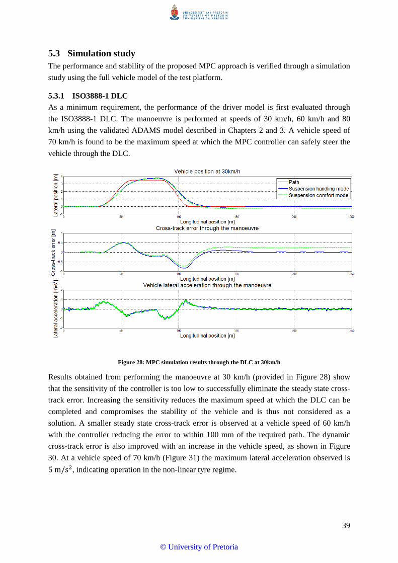
Figure 27 MPC simulation results through the DLC at 30kmh39
Figure 28 MPC simulation results through the DLC at 60kmh40
Figure 29 MPC simulation results through the DLC at 80kmh40
Figure 30 MPC simulation results through the DLC at 70kmh41
Figure 31 Indirect self-tuning regulator structure44
Figure 32 Indirect regulator simulation results through the DLC at 30kmh 46
Figure 33 Indirect regulator simulation results through the DLC at 60kmh 47
Figure 34 Indirect regulator simulation results through the DLC at 80kmh 47
Figure 35 Indirect regulator simulation results through the DLC at 88kmh 48
Figure 36 Indirect regulator simulation results through the DLC at 90kmh 48
copycopy UUnniivveerrssiittyy ooff PPrreettoorriiaa
VII
Figure 37 Indirect regulator RMSE through the DLC49
Figure 38 Indirect regulator parameter evolution through the DLC at 80kmh50
Figure 39 Indirect regulator simulation results through the sinusoidal path at 30kmh 51
Figure 40 Indirect regulator simulation results through the sinusoidal path at 60kmh 51
Figure 41 Indirect regulator simulation results through the sinusoidal path at 80kmh 52
Figure 42 Indirect regulator RMSE through the sinusoidal path52
Figure 43 Indirect regulator parameter evolution through the sinusoidal path at 80kmh 53
Figure 44 LQSTR structure 55
Figure 45 LQSTR simulation results through the DLC at 30kmh58
Figure 46 LQSTR simulation results through the DLC at 60kmh58
Figure 47 LQSTR simulation results through the DLC at 80kmh59
Figure 48 LQSTR simulation results through the DLC at 100kmh59
Figure 49 LQSTR simulation results through the DLC at 110kmh60
Figure 50 LQSTR simulation results through the DLC at 115kmh61
Figure 51 LQSTR RMSE through the DLC 62
Figure 52 LQSTR gain evolution through the DLC at 100kmh62
Figure 53 LQSTR simulation results through the sinusoidal path at 30kmh 63
Figure 54 LQSTR simulation results through the sinusoidal path at 60kmh 63
Figure 55 LQSTR simulation results through the sinusoidal path at 80kmh 64
Figure 56 LQSTR simulation results through the sinusoidal path at 100kmh 64
Figure 57 LQSTR RMSE through the sinusoidal path 65
Figure 58 LQSTR gain evolution through the sinusoidal path at 100kmh66
Figure 59 The positioning principle of GPS [54] 68
Figure 60 A gimbal based INS [55]70
Figure 61 Static drift time data 74
Figure 62 Static drift distribution74
Figure 63 Dynamic square test results 75
Figure 64 Yaw angle of the receiver during the dynamic square test76
Figure 65 DLCs measured with the SPAN-CPT 77
Figure 66 Reference position throughout testing day78
Figure 67 Adaptive controllersrsquo performance through the DLC 80
Figure 68 Adaptive controllersrsquo accuracy through the DLC 81
Figure 69 RMSE compared as a function of vehicle speed82
Figure 70 LQSTR structure with added integral action85
Figure 71 Illustration of offset at 90kmh in suspension handling mode 85
Figure 72 Simulated steering offset at 90kmh86
Figure 73 The test vehicle through the DLC manoeuvre87
Figure 74 Original vehicle position through the DLC manoeuvre 88
Figure 75 LQSTR implementation results through the DLC at approximately 40kmh 89
Figure 76 LQSTR implementation results through the DLC at approximately 60kmh 89
copycopy UUnniivveerrssiittyy ooff PPrreettoorriiaa
VIII
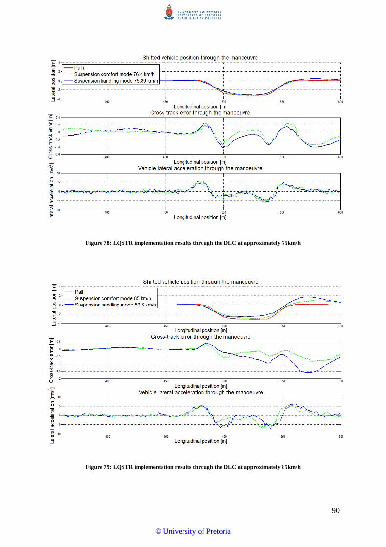
Figure 77 LQSTR implementation results through the DLC at approximately 75kmh 90
Figure 78 LQSTR implementation results through the DLC at approximately 85kmh 90
Figure 79 LQSTR implementation results through the DLC at 90kmh 91
Figure 80 LQSTR gains during implementation through the DLC at approximately 85kmh
92
Figure 81 LQSTR RMSE through the DLC during implementation plotted with the
simulated values92
Figure 82 RMSE values compared over all tested speeds 93
Figure 83 Oscillations caused by the integral action 94
Figure 84 Original vehicle position through the manoeuvre 95
Figure 85 The test vehicle on the dynamic handling track 96
Figure 86 Vehicle position and speed on the dynamic handling track 97
Figure 87 Vehicle position and cross-track error on the decreasing radius turns of the
dynamic handling track98
Figure 88 The test vehicle on the off-road test track 99
Figure 89 Off-road LQSTR implementation results through the DLC at approximately 455
kmh 99
Figure 90 Off-road LQSTR implementation results through the DLC at approximately 2631
kmh 100
Figure 91 Vehicle position and speed through the DLC along with the desired and actual
steering angles during the start-stop test 101
copycopy UUnniivveerrssiittyy ooff PPrreettoorriiaa
IX
List of Tables
Table 1 Vehicle transducers14
Table 2 Maximum relative error on peaks of correlation data [20]18
Table 3 Shillings findings on the yaw natural modes (Adapted from [48]) 30
Table 4 MPC and model parameters38
Table 5 Regulator and model parameters 45
Table 6 LQSTR and model parameters 57
Table 7 SPAN-CPT claimed accuracy (Adapted from [58])73
Table 8 LQSTR parameters during experimental validation84
copycopy UUnniivveerrssiittyy ooff PPrreettoorriiaa
X
List of Symbols and Abbreviations
List of Roman Symbols
Continuous pole location
Yaw acceleration
State space state matrix
Desired closed loop polynomial
Desired closed loop poles
Observer polynomial
Number of exogenous inputs
State space input matrix
Desired closed loop zeros
CG x-position in global axis system
CG y-position in global axis system
State space output matrix
ࢻ Cornering stiffness
Change in east-west Cartesian position
Cross-track error preview distance
Change in north-south Cartesian position
Path preview distance
Change in x coordinates
ᇱ Rotated change in x coordinates
Change in y coordinates
ᇱ Rotated change in y coordinates
Exponent
Value of eccentricity of the earth
Cross-track error
Model update frequency
Data sample frequency
Tyre longitudinal force
Tyre lateral force
ࢠ Tyre vertical force
Transfer function
Index subscript
LQSTR performance penalty function
MPC performance penalty function
Index subscript
Lateral gain
LQR controller gain
copycopy UUnniivveerrssiittyy ooff PPrreettoorriiaa
XI
Total wheelbase length
Number of least squares parameters
ࢠ Self-aligning moment
Samples delay
Path length
Blocking horizon
Control horizon
Prediction horizon
Number of data samples
Initial condition subscript
Number of autoregressive terms
Riccati solution
MPC performance weighting matrix
LQR performance weighting matrix
Equatorial radius
Polar radius
Input polynomial
Radius of the earth
Radius of a turn
MPC input weighting matrix
LQR input weighting matrix
Prime meridian
Prime vertical
Continuous transfer function variable
Feedback polynomial
Side force
Time
Setpoint polynomial
Controller input
Autoregressive input
Controller reference
Required side force
Transfer function denominator
Vehicle velocity
Freund controller filtered path
GPS satellite intersection
Vehicle velocity magnitude
Longitudinal position of the path in the
global axis system
State space state vector
copycopy UUnniivveerrssiittyy ooff PPrreettoorriiaa
XII
Measured plant output
State space output value
Predicted output
Transfer function numerator
Lateral position of the path in the global axis
system
State space output vector
෩ Predicted model output
Measured outputs
ࢠ Discrete transfer function variable
ࢠ Unit delay
copycopy UUnniivveerrssiittyy ooff PPrreettoorriiaa
XIII
List of Greek Symbols
ࢻ Slip angle
ࢻ Freund controller parameter
ࢼ Side-slip angle
ࢼ Normalising factor
Steering angle of wheels
Residual term
Damping ratio
Exogenous input weight
Least squares parameters
Longitude
Freund controller parameter
Freund controller tuning parameter
Lateral error preview time
Path preview time
Yaw rate preview time
Autoregressive weight
Latitude
Regression vector
Yaw angle
Actual yaw angle
Desired yaw angle
Yaw rate
Yaw rate setpoint
Natural frequency
copycopy UUnniivveerrssiittyy ooff PPrreettoorriiaa
XIV
List of Abbreviations
ACC Active Cruise Control
AR Auto Regression
ARX Auto Regression with eXogenous input
CA Collision Avoidance
CG Center of Gravity
DARPADefence Advanced Research Projects
Agency
DGPS Differential Global Positioning System
DLC Double Lane Change
DOP Dilution of Precision
EGNOSEuropean Geostationary Navigation Overlay
Service
FEM Finite Element Modelling
FLC Fuzzy Logic Controller
GLONASSGlobalnaya Navigatsionnaya Sputnikovaya
Sistema
GNSS Global Navigation Satellite System
GPS Global Positioning System
INS Inertial Navigation System
LIDAR Light Detection and Ranging
LQG Linear Quadratic Gaussian controller
LQR Linear Quadratic Regulator
LQSTR Linear Quadratic Self-Tuning Regulator
LR Left Rear
MPC Model Predictive Control
MRAC Model Reference Adaptive Controller
NFC Neuro-Fuzzy Controller
NHTSANational Highway Traffic Safety
Administration
NN Neural Network
PID Proportional Integral Derivative
RADAR Radio Detection and Ranging
RMSE Root Mean Square Error
RR Right Rear
SBAS Satellite-Based Augmentation System
SSE Sum of Squares Error
VDG Vehicle Dynamics Group
WAAS Wide Area Augmentation System
WGS 84 World Geodetic System revision of 1984
copycopy UUnniivveerrssiittyy ooff PPrreettoorriiaa
XV
4S4 4-State Semi-active Suspension System
copycopy UUnniivveerrssiittyy ooff PPrreettoorriiaa
1
Chapter 1
Introduction and Literature Survey
Throughout the existence of the automobile researchers have attempted to improve the safety
of all road users by augmenting the vehicle with support systems A driver model is a good
example of a system that could potentially save millions of lives if implemented on vehicles
as an augmentation during severe manoeuvres
11 Introduction
Vehicle automation has always been a very active research field usually aimed at increasing
the safety of the driver and occupants Manufactures such as BMW Mercedes-Benz and
Audi among others first started implementing intelligent system such as Radio Detection and
Ranging (RADAR) in the early 90rsquos [1] Although these early systems would only tension
seatbelts it was the first step to the advanced Collision Avoidance (CA) systems of today
Modern CA systems employ a variety of techniques aimed at improving the safety of the
vehicle These include assistive braking and Active Cruise Control (ACC) all of which is
designed to control the distance between the vehicles Although extensive research has been
done on longitudinal CA lateral CA has largely been limited to driver feedback and other
warnings Statistics by the National Highway Traffic Safety Administration (NHTSA) of the
USA show that head on and rear-end collisions make up 343 of the total number of
collisions while angled and sideswipe collisions make up 325 Despite this head on and
rear-end collisions are responsible for only 153 of all collision fatalities while angled and
sideswipe collisions are responsible for 203 of all collisions fatalities Furthermore a total
of 217 of all fatal collisions occurred while the vehicle was negotiating a curve [2] These
numbers demonstrate the effectiveness of longitudinal CA systems and emphasize the need
for a lateral CA system as no active systems are currently available
Lateral CA systems can be divided in two groups
1 Object detection and avoidance strategy (known as path planning)
2 Following a predetermined path to avoid an identified obstacle (known as path
following)
Extensive work has been done on object detection algorithms and avoidance strategies for
automotive applications employing visual or scanning sensors Researchers from the
Technische Universitaumlt Darmstadt in Germany developed a collision avoidance system
known as PRORETA [3] The system utilizes a fusion of Light Detection and Ranging
(LIDAR) and camera data to detect a possible collision with another vehicle Upon
copycopy UUnniivveerrssiittyy ooff PPrreettoorriiaa
2
triggering the system either reduces the vehicle speed or calculates an evasive trajectory in
an attempt to prevent the collision Another example of such a system with path following
capabilities was developed by Yoon et al and utilizes a model-predictive controller to steer
the vehicle on the calculated path [4] Despite being able to detect obstacles and plan
avoidance trajectories these systems normally rely on the assumption of linear vehicle
dynamics leading to inadequate performance at higher vehicle speeds and during severe
manoeuvres
Path following systems are responsible for determining the vehicle steering input required to
follow a predetermined path with minimal deviation These systems are designed using a
driver model which characterises the lateral response of a vehicle to some input (usually a
lateral position error or trajectory error) and may also be termed a steering controller
Although many models exist few have been successfully validated at highway speeds and
high lateral accelerations where the effect of the non-linear tyre-road interface becomes
significant Among the few that does consider the non-linear response effects in this regime is
the non-linear model described by Edelmann and Ploumlchl which uses a preview controller [5]
Gain scheduling can be used to allow these types of controllers to compensate for the non-
linearity at higher lateral accelerations by linearizing about a range of operating points Not
only are these controllers limited to a specific operating environment determining the various
gains that deliver stable performance proves to be a tedious process
Some models attempt to physically model the vehicle using a set of parameters as opposed to
determining the transient response of the system empirically This is demonstrated by the
driver model developed by Canale et al [6] Physical models are usually computational
complex and cannot be used on-line to control the vehicle They also require parameters that
cannot be easily determined while the vehicle is in operation (such as the position of the
center of mass) which poses a problem for practical control of a vehicle
In an effort to model the tyre-road interface and its non-linearity Bakker and Pacejka
proposed the Magic Tyre Formula [7] The formula performs a curve fit on measured data to
characterize the forces generated by the tyre and has been used by many to develop non-
linear driver models While providing satisfactory results on manmade surfaces the curve fit
coefficients are only valid in the environment that the initial measurements were performed
in When the vehicle is driven in different conditions the controllers must rely on their
disturbance rejection properties to follow the required path
Thus there exists a need for a robust driver model that can compensate for the non-linear
dynamics of the vehicle at high lateral accelerations without being bound to a specific
operating environment
copycopy UUnniivveerrssiittyy ooff PPrreettoorriiaa
3
12 Non-linearity in vehicle dynamics
When considering the vehicle system many non-linear components can be identified This
ranges from a non-linear engine curve and backlashing of gears in the driveline to the
temperature dependent deceleration of the wheels during braking Perhaps the largest
contributor to the non-linearity of vehicle dynamics is the tyre-road interface and the manner
in which lateral force is generated by a rolling tyre
A rolling tyre generates lateral force by manner of deformation Figure 1 demonstrates this
effect in which the alignment of the contact area of the tyre is offset by an angle from the
longitudinal axis of the tyre This angle is more commonly known as the side-slip angle At
low side-slip angles the lateral deformation of the tyre is minimal and almost no lateral force
is generated However as the side-slip angle increases so does the amount of lateral force
Figure 1 The side-slip angle of a tyre [8]
Figure 2 shows plots of lateral force vs side-slip angle and longitudinal force vs longitudinal
slip to demonstrate the non-linearity present in the tyre-road interface
Figure 2 Typical lateral and longitudinal force generation of a tyre under different vertical loads [9]
copycopy UUnniivveerrssiittyy ooff PPrreettoorriiaa
4
The lateral force generation of the tyre is mostly linear at low slip values but becomes non-
linear as the amount of side-slip increases and the lateral force saturates A similar
observation can be made when considering the longitudinal force generation where a
maximum is reached at approximately 20 slip It should also be noted that the amount of
force generated and the point at which the lateral force saturates is largely dependent on the
vertical load of the tyre This implies that vehicle roll pitch and general load-transfer
between the wheels of the vehicle add to the non-linearity of the problem
Many have attempted to model the tyre-road interface with varying levels of success
Existing tyre models can be classified as physical semi-empirical or empirical models and
can model either the force generation or the vertical dynamics of the tyre As this study does
not consider ride comfort only the lateral and longitudinal force generation aspects will be
discussed
Physical tyre models are also known as white box models and attempt to describe the force
generation of the tyre by means of physical laws and wheel-ground interaction models These
models are known to be very complex and take some time to solve making them impractical
for online applications [10] These include Finite Element Modelling (FEM) based models
Contrasting this is the so-called black box or empirical models in which a range of
measurements are taken and used to construct a lookup table Although this could provide a
simple quick solving solution the conditions in which such a model is valid are limited
The most popular modern tyre model is an example of a grey box or semi-empirical model
The Pacejka Magic Tyre Formula [7] performs a curve fit to measured data in an effort to
describe the tyre-road interface Although similar to the black box approach the coefficients
used were chosen to have some physical meaning thereby easing the task of identifying the
initial model parameters Having some initial parameters eases the task of optimizing the
curve fit The model is however still only valid on man-made surfaces similar to those on
which the original data was obtained although the estimated friction coefficient can be
adjusted in the curve fit parameters
13 Driver models
A wide range of driver models have been developed in the past These range from human
based models which emulate the biological response and neuromuscular delays of the driver
to advance physical models based solely on the geometry and dynamics of the vehicle Work
has also been done on developing behavioural driver models which try to replicate the human
thought and learning processes and incorporate it into the control of the vehicle
131 Vehicle based driver models
Vehicle based driver models can be divided into three categories (with increasing
complexity) geometric models kinematic models and dynamic models Conventionally in-
plane geometric and kinematic models are favoured for their simplicity As this simplicity is
copycopy UUnniivveerrssiittyy ooff PPrreettoorriiaa
5
achieved by neglecting the effect of slip these models tend to become less accurate during
higher lateral accelerations in the non-linear tyre regime Dynamic models based on
Newtonrsquos second law of motion are preferred in this instance
Geometric and Kinematic Driver Models
Geometric driver models are designed by taking into account only the geometry of the
vehicle more specifically the wheelbase and steering angle that allows the vehicle to move
on a constant radius A geometric controller incorporates no additional information about the
vehicle being controlled
An example of a geometric driver model is the pure pursuit method based on simplified
Ackerman steering geometry The pure pursuit method calculates the steering angle required
to have the rear wheel intersect a predetermined goal point on the path assuming a constant
radius curvature and a specified preview distance [11] An illustration of the pure pursuit
model is shown in Figure 3 along with the Stanley method path follower Stanford
University developed the Stanley method based on their autonomous vehicle competing in
the Defence Advanced Research Projects Agency (DARPA) Grand Challenge [12] Stanley
the autonomous Volkswagen Touareg won the 2005 DARPA Grand Challenge using the
Stanley method controller to steer the vehicle The Stanley method controller regulates the
heading of the vehicle and incorporates a non-linear penalty function to minimize the cross
track error
A study performed by Snider using the CarSim software package and a simple proportional
controller with the geometric driver models showed that reasonable path following can be
achieved at low speeds [13] It was however found that the controller gains used caused it to
become unstable at higher speeds and had to be re-tuned to achieve path following at these
speeds This illustrates the compromise between path following accuracy at low speeds and
high speed stability when using geometric driver models
Figure 3 The Pure Pursuit model (left) and the Stanley model (right) [13]
copycopy UUnniivveerrssiittyy ooff PPrreettoorriiaa
6
A kinematic driver model can be considered the most basic form of a vehicle model These
driver models are based on the linear equations of motion and operate under the assumption
of no wheel slip Figure 4 illustrates the kinematic bicycle model (also referred to as a yaw
planar model) in which the left and right tyres are represented as one with the average
steering angle at the front wheel
Figure 4 A kinematic driver model [13]
Kinematic models use the steering angle and vehicle geometry to calculate the vehicle
velocity component in each direction as well as the in-plane rotation of the vehicle Simple
integration yields the estimated position of the vehicle Apart from the wheelbase of the
vehicle no additional vehicle dynamics are incorporated in the models Although kinematic
driver models yield better results at low speed than their geometric counterparts a trade-off
between path following accuracy and path following speed is still required when using a
single gain controller
Dynamic Driver Models
Unlike the geometrical and kinematic driver models dynamic driver models do not disregard
the tyre-road interface Instead the response of the vehicle is estimated by considering the
dynamics of the vehicle system either explicitly through mathematical equations or through
intelligent system techniques such as neural networks (NN) The introduction of the
additional dynamics does however increase the complexity of the system and the
computational effort required to solve it In an attempt to reduce this complexity many
models linearize the dynamics of the tyre-road force generation Although satisfactory results
are achieved at low to medium lateral accelerations the non-linear tyre force generation and
tyre force saturation causes these models to deviate significantly at high lateral accelerations
Basic driver models use Newtonrsquos second law and the forces generated by the tyres directly
to estimate the vehicle acceleration and yaw-rate A simple dynamic model is formulated by
expanding the bicycle model discussed earlier and is illustrated in Figure 5 [13] Here the
copycopy UUnniivveerrssiittyy ooff PPrreettoorriiaa
7
introduction of tyre forces and vehicle dynamics to the model allows the concept of side-slip
and tyre slip angles to be addressed Ackermann et al developed a similar dynamic driver
model for the lateral control of a city bus [14] The model incorporated vehicle dynamics
such as slip but the tyre-road interface was modelled using the linear tyre model of Riekert
and Schunck [15] and was found to be valid only at low lateral accelerations
Figure 5 A simple dynamic driver model
In an attempt to overcome the instabilities of the controllers at high speeds caused by
linearization of the tyre-road interface many researchers proposed sliding-mode control as a
solution In a sliding-mode algorithm the control structure is modified based on the current
state of the system In other words more than one controller is designed and the correct
variant is selected based on the lateral acceleration of the vehicle This was implemented by
Ackermann at al as a successor to the initial linear city bus controller discussed earlier
Ackermann found that although no noticeable difference was observed in controller settling
time the sliding-mode controller yielded smaller deviations from the set guideline than the
previous linear controller [16]
Falcone et al proposed a Model Predictive Control (MPC) scheme for the active steering
control of a vehicle [17] The controller was based on a non-linear vehicle model as opposed
to the linear model of Yoon et al [4] and tasked with determining the optimal steering angle
The steering angle was required to steer the vehicle with a calculated trajectory and was
implemented over a finite preview horizon Results showed that as with many optimal
control problems the computational complexity of the optimisation limited the
implementation to very low vehicle speeds This was overcome by implementing a low order
linear time varying controller designed to perform online linearization of the vehicle model
Despite being able to stabilize the vehicle at speeds of up to 21 ms the controller is based on
a detailed vehicle model and cannot be easily transferred to a different platform Furthermore
the non-linear tyre-road interaction is based on the Magic Formula tyre model [7] While this
copycopy UUnniivveerrssiittyy ooff PPrreettoorriiaa
8
model provides a good approximation of the tyre characteristics on manmade surfaces it is
limited to the surface on which the initial model was generated
Sharp et al suggested a modified optimal controller that utilises more than one preview point
[18] The multi-point preview approach allows the controller to weigh each error
appropriately along with the current state feedback in order to determine the required steer
angle The introduction of saturation functions in the model attempts to mimic the tyre force
saturation that occurs during vigorous manoeuvring Even though these gain parameters are
difficult to tune Sharp notes that although the system is based in linear optimal control
theory the structure is similar to that of a NN He argues that the model parameters can be
found using NN learning approaches This indicates that the use of intelligent system
techniques might be necessary to capture the highly non-linear dynamics present in the lateral
control of a vehicle
Neural networks are designed to mimic the learning response of a human to a specific
situation by using a set of training data and identifying input-output scenarios The possibility
of using a NN as a driver model was already investigated in the early 90rsquos as demonstrated
by the NN steering controller of Mecklenburg et al Although the controller was trained
offline using a linear plant model simulations proved it superior to the classical vehicle
control techniques of the time [19] A feedforward NN was also used by Botha to characterise
the steering angle required to steer a test vehicle with a specified yaw rate at a certain vehicle
speed Results from the study showed that performance similar to the mathematical model
could be achieved at a fraction of the computational cost [20] However as the model was
trained using the Inverse Magic Formula proposed by Thoresson [21] its performance is
limited by its operating environment and is bound to the test platform used
A drawback of NNs is the amount of training data required to successfully develop the
system The response of a NN is also limited to the scope of training data used and cannot
handle situations that the system was not trained for In many cases especially when training
a vehicle controller the gathering of training data can be a time consuming and unpractical
process A compromise has been proposed in the form of Fuzzy Logic Controllers (FLC)
The concept of fuzzy logic has already been introduced in the 60rsquos by Zadeh [22] but only
became popular in the late 80rsquos FLCs attempt to mimic human reasoning by moving away
from precise measurements and by labelling a situation in a so-called lsquofuzzy mannerrsquo These
controllers are known for being able to control complex non-linear systems of which a
mathematical model is not easily available through the use of linguistic techniques
Conventional FLC implementations was limited to basic tasks such as determining optimal
settings for household appliances based on load parameters [23] The use of FLCs as vehicle
support systems was suggested by Li et al who implemented a FLC as a stability control
system A FLC was used to minimise the side slip angle of the vehicle during a range of
steering manoeuvres [24]
copycopy UUnniivveerrssiittyy ooff PPrreettoorriiaa
9
Hessburg and Tomizuka showed that a FLC delivered the same performance as a
conventional Proportional Integral Derivative (PID) controller when autonomously
performing manoeuvres up to 50 kmh [25] While the PID loop was tuned using an explicit
linear vehicle model the FLC was designed using an implicit model and contained only
simple logic instructions Another comparison with a conventional PID system was done by
Kodagoda et al who proposed a FLC based on variable structure systems theory applied to
the control of an electric golf cart Results from this study showed the FLC to outperform
conventional PID control in both tracking and robustness The study indicated that the lateral
FLC can be implemented along with a longitudinal FLC without any coupling between the
systems while still maintaining the robustness of the individual controllers [26]
Even though FLCs are capable of controlling non-linear systems the construction of the
membership functions that lead to a stable response can be a tedious process To overcome
this a neuro-fuzzy controller (NFC) was first proposed by Lee and Berenji [27] The purpose
of the NFC is to modify the membership functions through machine learning much like a
human operator would modify inputs to the system based on previous experiences This
increases the robustness of the controller as demonstrated by Perez et al who implemented a
NFC to perform the longitudinal control of a gasoline vehicle [28] Lateral control of a
vehicle using a NFC has been performed in a study by Ryoo and Lim where the NFC was
tasked with following the curvature of a road [29] Despite the fact that this was demonstrated
using a small wheeled robot at low speeds the path following capabilities of the system
proved promising A different study by Ting and Lui showed that a NFC is superior to a
conventional linear controller at high vehicle speeds where the tyre-road interface becomes
non-linear [30]
Adaptive controllers are frequently implemented to deal with a non-linear process model and
have been successfully implemented in ship navigation [31] Similar to the sliding mode
controllers discussed earlier an adaptive controller evolves according to the current state of
the plant Peng and Tomizuka suggested an adaptive controller in the form of a frequency-
shaped linear quadratic controller of which the performance function is modified to include
factors such as ride quality and robustness to wind gusts The controller was designed using a
linearized vehicle model [32] An adaptive lateral vehicle controller was also designed by
Netto et al [33] The controller was constructed using self-tuning regulator theory and a
vehicle model proposed by Ackerman containing a set of bounded uncertain vehicle
parameters Simulations showed a robust response up to 25 ms (90 kmh) with minimal
deviations from the setpoints Similar to Nettorsquos driver model Fukao et al suggested a Model
Reference Adaptive Controller (MRAC) to solve the active vehicle steering problem [34]
The MRAC approach was also followed by Byrne and Abdallah who design and verified a
MRAC on a vehicle road following in simulation [35] During the study Byrne noted that the
saturation of the steering angle posed a problem when using MRAC theory which in turn
required the adaption gains to be adjusted Although promising results were achieved the
copycopy UUnniivveerrssiittyy ooff PPrreettoorriiaa
10
analysis was based on a simple bicycle model for speeds up to 25 ms and remains to be
verified experimentally
Although these driver models attempt to compensate for the non-linear dynamics of the
vehicle with varying rates of success all are designed using a fixed vehicle model This
implies that any significant changes in the vehicle parameters or operating environment are
treated as disturbances and may impact the performance of the controller In order to
successfully account for the non-linear dynamics the effect of the environment on the vehicle
needs to be included in the vehicle model
132 Human based driver models
Human based driver models are generated by considering the human driver as a controller
responsible for safely operating the vehicle This leads to models that consider common
biological limitations such as the neuromuscular time delays and threshold limitations [36]
Emphasis is also placed on the sensory aspects of human modelling including visual
vestibular auditory and tactile information Some of these driver models even attempt to
model driver skill as a response to task difficulty and try to emulate the actual sub-optimal
response of a human being
The sub-optimal nature of these models is not ideal when considering autonomous systems
as the purpose of an autonomous vehicle controller is to improve the safety and performance
of the vehicle above the capabilities of the conventional driver Despite these attributes a
human driver is able to adapt to different driving conditions and use a preview of the path to
anticipate future control moves A model of this adaptive control behaviour can prove useful
in an autonomous vehicle controller as it is not bounded by its operating conditions
133 Behavioural driver models
The concept of behaviour driver models is generally ill defined and is usually included in
dynamic or human based driver models It is described by Abe and Manning as the human
driverrsquos ability to adjust its control and sensing strategy according to the current vehicle
parameters [37] For example as the vehicle speed increases a human driver would increase
the preview distance and decrease the severity of steering inputs to the vehicle This is similar
to the FLCs NFCs and sliding mode controllers discussed earlier but is more heavily based
on human reasoning than on prior knowledge of basic vehicle dynamics However as human
reasoning is difficult to define mathematically most designers prefer the more structured
approach of FLCs and NFCs to solve the path following problem using human-like logic
copycopy UUnniivveerrssiittyy ooff PPrreettoorriiaa
11
14 Conclusion
A ground vehicle is a dynamic system containing many non-linear components ranging from
the non-linear engine response to the tyre-road interface Extensive work has been done in an
attempt to model and control the vehicle system utilising a wide variety of conventional
control and intelligent systems theory
The use of geometric and kinematic driver models are found to be inadequate while the
majority of dynamic driver models are based on linear vehicle dynamics and are limited to
either low speed or high speed applications respectively This can be attributed to the non-
linear tendency of the tyre-road interface at high lateral accelerations as conventional linear
control struggles to capture the tyre force saturation that occurs in this region Thus a
compromise is required between low speed accuracy and high speed stability when
implementing conventional driver models Current driver models are also sensitive to
changes in the vehicle parameters as well as the operating environment of the vehicle
Although some models do account for the non-linearity in an attempt to facilitate low speed
and high speed path following these are found to be either computationally inefficient or to
require a vast amount of training data to synthesize The use of FLCs as driver models seems
promising but in-depth knowledge of the problem is required to set up the required fuzzy
rules and proves to be a tedious design process Adaptive control adapts the control action
according to the current state of the process and is largely dependent on an accurate estimate
of the plant model Up to date only linear models have been used to implement adaptive
control in the field of vehicle dynamics
The gap in lateral driver models has limited the progress made in the development of lateral
CA systems which could potentially reduce the number of fatalities caused by vehicle
collisions It can thus be concluded that a need exists for a robust driver model capable of
performing path following at both low and high lateral accelerations through the non-linear
tyre regime without being sensitive to changes in vehicle parameters and operating
environment Development of such a driver model would aid the design of lateral CA
systems thereby increasing the safety of all road users
15 Research focus
It is evident from the literature reviewed that more work is necessary in the field of lateral
CA systems as the current available driver models are limited by the non-linearity of the
tyre-road interface Although some do account for this non-linearity these models are
normally based on a semi-empirical model restricting the operating environment of the
vehicle This study aims at developing a driver model that allows an off-road vehicle to
perform robust path following in different environments assuming that the required path is
known a-priori
copycopy UUnniivveerrssiittyy ooff PPrreettoorriiaa
12
The resulting driver model will use an implicit vehicle model to account for the non-linearity
at high lateral accelerations It should be able to perform stable path following at both low (lt
60 kmh) and high vehicle speeds (gt 70 kmh) The driver model should be able to safely
steer the vehicle through manoeuvres resulting in high lateral accelerations (gt 4 msଶ) in
the non-linear tyre force regime
Development of the driver model will be done by considering various adaptive controllers
each following a different approach in controlling a non-linear process The performance of
these controllers will be evaluated in simulation after which the best performing controller
will be implemented and validated experimentally
Although Electronic Stability Control (ESC) systems are common on modern vehicles and
can improve their handling characteristics this study is performed without such a system
This is not only done to ensure better repeatability of tests as the ESC system might not react
in the same manner each time but also because the experimental vehicle used in this study is
not fitted with an ESC system The adaptive nature of the proposed control algorithms should
however also allow implementation on vehicles with ESC systems as the response of the
vehicle is determined on-line by considering measured input-output data This captures the
response of the vehicle with the effect of its driving aids includedExperimental validation is
done by autonomously performing amongst others an ISO3888-1 severe Double Lane
Change (DLC) [38] To achieve the required lateral acceleration the test will be performed at
the same speed at which an experienced human driver can complete the task in the test
vehicle Evaluation of the driver model performance is done using both the overall stability of
the vehicle and the driver model as well as the path following accuracy that can be achieved
copycopy UUnniivveerrssiittyy ooff PPrreettoorriiaa
13
Chapter 2
Vehicle Platform and Multi-Body Dynamics
Model
This study is performed using a Land Rover Defender 110 TDi from the Vehicle Dynamics
Group (VDG) of the University of Pretoria The test platform has been used in various studies
performed by the group including the development of a full vehicle model in MSC ADAMS
by Thoresson [21] and Uys et al [39] A model of the platform will be used extensively in
developing and testing a robust driver model for the vehicle and is also discussed in this
section Validation of the driver model will be done experimentally using the instrumented
Land Rover Defender fitted with the controller hardware and software
21 Test platform
The Land Rover Defender 110 of the VDG is equipped with various systems that enable
modification of the vehiclersquos dynamics as well as measurement equipment These will be
reviewed in this section
211 4S4 Suspension system
In an effort to improve the ride-handling compromise Els [40] developed the 4-State Semi-
active Suspension System (4S4) hydro-pneumatic suspension system This system enables
switching between a ride mode (soft spring and low damping) and a handling mode (stiff
spring and high damping) The ride mode settings have been optimised for ride comfort
ignoring handling requirements Handling mode on the other hand has been optimised for
handling and reduced roll-over propensity and result in an uncomfortable ride over rough
terrain The ride and handling settings therefore lie at opposite ends of the design spectrum
and are vastly different By automatically switching between a handling mode with high
spring stiffness and damping and a comfort mode utilising low spring stiffness and damping a
compromise is found between ride and handling using a single suspension system The 4S4 is
also capable of switching between four discrete spring-damper combinations on each
suspension strut This versatility will be used to modify the yaw response of the test platform
and will aid in determining the robustness of the driver model
212 Vehicle instrumentation
Although the test platform is equipped with various sensors only those pertaining to the
lateral dynamics of the vehicle and the measurements required by the driver model will be
considered in this section These are tabulated in Table 1 for reference Figure 6 provides the
locations of the sensors on the test platform The vehicle position is provided by a global
positioning system (GPS)
copycopy UUnniivveerrssiittyy ooff PPrreettoorriiaa
14
Table 1 Vehicle transducers
Measurement Transducer
Vehicle position
SPAN-CPT (NovAtel)
Vehicle heading
Vehicle speed
Vehicle yaw rate
Vehicle lateral acceleration
CG lateral acceleration Crossbow accelerometer
Steering kingpin angle Absolute encoder (Eltra)
Figure 6 Transducer locations on the vehicle platform (Image adapted from [41])
213 Control system hardware
Figure 7 provides the proposed structure for the implementation of the control system on the
vehicle platform The analogue signals from the absolute encoder and CG accelerometer are
passed directly to the processing block while the SPAN-CPT measurements are transferred
using RS-232 serial communication All processing including sampling of the required
analogue channels and providing the analogue control signal to the steering motor controller
is performed using a Helios single board computer from Diamond Systems [42] running a
Slackware version of Linux The Helios computer is powered using the on-board 12V power
supply and contains a Vortex86DX CPU running at 1GHz as well as 256MB RAM The on-
board input-output interfaces available include RS-232 serial ports sixteen single-ended 16
bit analogue to digital converters four 12 bit digital to analogue converters and forty general
purpose digital input-output pins This should provide enough computing power as well as
sampling capabilities to successfully implement and test a driver model experimentally
copycopy UUnniivveerrssiittyy ooff PPrreettoorriiaa
15
Figure 7 Block diagram of controller hardware
Actuation of the steering system is done using a FESTO EMMS-ST-87L stepper motor
controlled by a FESTO CMMS-ST-G1 stepper motor controller in analogue tracking mode
[43] The steer angle of the front wheels (referred to as the steer or steering angle in this
study) is driven through a belt system on the steering column using the stepper motor In
analogue tracking mode the speed and direction of the stepper motor is set proportional to the
reference voltage allowing the use of the proportional steer rate controller discussed in the
next section of this report
Installing the stepper motor in parallel with the existing steering system allows driver
intervention should a malfunction occur The actuator system is depicted in Figure 8 while
Figure 9 illustrates the system installed in the vehicle The steering actuator is able to achieve
a maximum steer rate of ͳͷιȀݏ while the steer angle of the vehicle is mechanically limited to
30deg to each side by the steering geometry These parameters are also included in the
simulation to allow for an accurate representation of the real vehicle
Figure 8 Stepper motor assembly [20]
copycopy UUnniivveerrssiittyy ooff PPrreettoorriiaa
16
Figure 9 Top view of the stepper motor assembly installed in the engine bay
22 Vehicle model
The vehicle is represented in simulation using a 16 degree of freedom non-linear model in
MSC ADAMS Development of the model was done using experimentally determined body
torsion moments of inertia and suspension characteristics The spring force of the hydro-
pneumatic suspension is modelled using diabatic process theory while the dampers and
bump stops are modelled using look-up tables A representation of the full vehicle model as
shown in ADAMS is provided in Figure 10
The tyre-road interface is modelled using the Pacejka lsquo89 tyre model [44] fitted using data
obtained by Thoresson [21] This is incorporated into the model using the ADAMS Tyre
package It should be noted that the self-aligning moment and longitudinal characteristics of
the tyre are excluded from the model to keep the model simple and to decrease the solving
time
The suspension kinematics is modelled using solid axles and joints similar to those found on
the test platform as shown in Figure 11 and Figure 12 It consists of a leading arm front
suspension system with a Panhard rod while the rear suspension is constructed using trailing
arms A single A-arm constrains the rear axle laterally The torsional spring in the model
represents the effect of the front anti-roll bar of the vehicle
copycopy UUnniivveerrssiittyy ooff PPrreettoorriiaa
17
Figure 10 ADAMS vehicle model [20]
Figure 11 Model front suspension [20]
copycopy UUnniivveerrssiittyy ooff PPrreettoorriiaa
18
Figure 12 Model rear suspension [20]
The full vehicle model is implemented in Simulink using an ADAMS controls plant for co-
simulation This is done to easily include the non-linear suspension characteristics of the 4S4
suspension system and to streamline the process of developing a steering controller through
simulation
Validation of the vehicle model used was performed in a study by Botha [20] in which a
series of DLC [38] manoeuvres were performed at various speeds both experimentally and in
simulation using the ADAMS vehicle model The values are compared using a maximum
relative error approach where the maximum discrepancy between the simulated and
measured data in expressed as a percentage of the measured value Upon comparing the
experimental and simulation results Botha concluded that the vehicle model is an accurate
representation of the test platform for use in vehicle handling studies Botha did note that the
suspension friction is not accurately modelled and may cause the model to deviate from
experimental results but argued that this should not be a problem in handling studies and can
be eliminated by performing a vertical shift on the data A summary of the correlation data as
compiled by Botha is provided below for reference
Table 2 Maximum relative error on peaks of correlation data [20]
Maximum Relative Error []
SpeedYaw
Rate
Yaw
Angle
Lateral
Acceleration
Suspension
Force RR
Suspension
Displacement
LR
Path
55kmh 1607 1506 1700 1067 60 516
735kmh 505 027 1538 767 2620 720
copycopy UUnniivveerrssiittyy ooff PPrreettoorriiaa
19
Simulation of the vehicle model is performed using a co-simulation setup between MSC
ADAMS and Simulink Figure 13 illustrates the input communicated and measured variables
in the simulation used to verify and validate the driver models The driver model and
suspension characteristics are solved in Simulink while the multi-body dynamics is solved in
MSC ADAMS Measurements are also performed in Simulink
Figure 13 Simulation structure overview
23 Conclusion
Access to a validated full vehicle model implemented using ADAMS and Simulink co-
simulation eases the process of developing a driver model and allows efficient debugging of
the system before it is implemented experimentally The good correlation between the vehicle
model and the test platform also implies that the developed model can be transferred to the
platform without modification of the algorithm This validated full vehicle model will be used
in the development of an intelligent driver model capable of performing autonomous path
following
The fully instrumented vehicle test platform allows experimental validation of the robust
driver model on various terrains some which cannot be accurately modelled in software
Implementation of the driver model in the presence of random noise and disturbances also aid
in determining the robustness of the controller Lastly implementation of the driver model on
the test platform in real-time should support the feasibility of a lateral CA system based on
this driver model
copycopy UUnniivveerrssiittyy ooff PPrreettoorriiaa
20
Chapter 3
General driver model structure and
performance evaluation methodology
Successful comparison of the adaptive strategies requires a set structure and testing
procedures This section provides an overview of the general driver model approach used in
this study as well as the methodologies used to determine and quantify the performance of
the adaptive controllers
31 Driver model structure
The general structure of the driver model used to verify the performance of the adaptive
controllers will be discussed here Some important parameters are also defined in this section
311 Overview
Vehicle path following can be separated into two control problems yaw angle control and
lateral position control In order for the vehicle to perform stable path following yaw angle
control is responsible for aligning the vehicle with the heading of the required path This
prevents oscillation of the vehicle around the path and a potentially unstable situation The
second controller is of secondary importance and is tasked with removing small lateral offsets
or cross-track errors that might arise during a dynamic manoeuvre The errors and yaw angles
of importance are defined in Figure 14
Figure 14 Definition of the desired yaw and lateral error parameters
Figure 15 demonstrates the general structure that will be used during the implementation of
adaptive control on the vehicle platform A yaw angle reference is passed to the driver model
copycopy UUnniivveerrssiittyy ooff PPrreettoorriiaa
21
after which the estimator and adaptive controller attempts to safely achieve this The lateral
control of the vehicle is incorporated through a proportional controller that adds to the yaw
reference signal This strategy prevents the possibility of contradicting controllers which may
occur if separate controllers are implemented for yaw and lateral position control Through
various simulation runs it was determined that the optimal proportional gain for the lateral
error is 1degm when a preview of 01s is used
Figure 15 Driver model layout
As opposed to controlling the yaw angle directly the yaw rate of the vehicle is controlled
This is discussed in more detail in Chapter 4 The conversion from yaw angle to yaw rate is
performed assuming a constant acceleration over a small period of time allowing the use of
the general equation of motion for the rotation of a rigid body in plane motion provided in
equation (1)
Δ =
ݐΔݐ+
1
2
ଶ
ଶݐΔݐଶ (1)
The controller block is defined in the following chapters as the structure of this block varies
according to the type of adaptive strategy used Figure 16 depicts the general steering
actuator control approach for the vehicle that will interface with the designed driver models
Figure 16 Steering actuator control structure
A steering rate controller is implemented using proportional control in conjunction with the
FESTO stepper motor controller previously discussed This allows for a quick responding
steering controller that should provide a steer angle with minimal offset and oscillation This
also ensures that the steering actuator control is much faster than the vehicle dynamics of the
vehicle and should thus not influence the adaptive control strategy of the driver model
copycopy UUnniivveerrssiittyy ooff PPrreettoorriiaa
22
312 Model preview
Preview is required in the driver model due to restrictions in the movement of the vehicle ie
the vehicle needs to move longitudinally to change its heading and lateral position The
structure of the driver model requires three previews (see Figure 14) These are the path
preview the lateral error preview and the yaw rate preview The values for these preview
distances are speed dependent and are defined as a time constant to allow for adjustment with
vehicle speed
The path preview is used to determine the yaw reference while the lateral error preview
indicates where the projected lateral error should be calculated The yaw rate reference is
used in the general equation of motion to determine the yaw rate required to achieve the
desired yaw angle some point in the future As these are expected to be different for each
adaptive strategy the values are quoted along with the adaptive controller parameters in the
following chapters
32 Performance evaluation
The performance of the driver model is evaluated using two criteria vehicle stability and path
following accuracy Vehicle stability is regarded as the primary objective and path following
accuracy is allowed to be sacrificed (within reason) to safely complete a desired manoeuvre
without inducing rollover Navigating the ISO3888-1 DLC [38] safely is set as the minimum
performance requirement for a driver model
321 Stability
The stability of the driver model is not only defined by safely navigating a required
manoeuvre but also by its ability to move in a straight line without constant oscillations of
the steering andor yaw angle Both these requirements will be evaluated visually after the
vehicle has navigated the evaluation paths At low speeds steady state oscillations are
particularly unwanted while the high speed stability will be under consideration for speeds
greater than 60kmh
322 Path following accuracy
The path following accuracy of the controllers is evaluated using both the maximum path
deviation and the lateral root mean square error (RMSE) in the global axis system throughout
the manoeuvre A higher RMSE will point to a worse average path following performance
while the maximum path deviation provides an indication of the dynamic cross-track
accuracy of the system The RMSE is given by equation (2)
ܯ ܧ =ඩsum ቆminቆට൫ݕ௧minus ௬
൯ଶ
+ ൫ݔ௧minus ௫൯ଶቇቇ
ଶ
ேୀଵ
(2)
This error is not determined at a preview distance as required by the controller but rather
taken as the lateral deviation of the vehicle CG from the path Doing so eliminates the effect
copycopy UUnniivveerrssiittyy ooff PPrreettoorriiaa
23
of the vehicle heading on the lateral error value The RMSE will also only be considered in
stable cases as sliding out of the vehicle will skew the RMSE value
323 Vehicle speed through the manoeuvres
As the driver model should be able to safely steer the vehicle in all operating conditions the
adaptive controllers will be tested at low as well as high speeds For low speed driving a
speed of 30 kmh will be used to evaluate the performance of the driver model Here the path
following accuracy and steady state stability are of main concern An intermediate speed of
60 kmh will also be considered representing the transition zone where the vehicle dynamics
are non-linear when driving on a conventional tar road with the test platform High speed
steering will be done at 80 kmh
In the saturation region of the tyre high speed stability of the vehicle is more important
Should the driver model be able to successfully complete the manoeuvre at 80 kmh the
vehicle speed will be incrementally increased to determine the highest safe operation speed of
the adaptive controller when used in the driver model structure
324 Evaluation of controller robustness
Robustness of the controllers is a crucial requirement in evaluating the performance of the
system in different environments and on varying surfaces The vehicle dynamics of the test
platform are modified using the semi-active suspension (4S4) fitted to the vehicle By
switching the suspension between the handling mode and comfort mode configurations the
vehicle dynamics can be varied sufficiently to show the robustness of the particular
controller The largely different yaw responses observed between the handling mode and
comfort mode setting poses a challenge to most driver models Thus the simulations and
validation experiments will be performed using both the handling mode and comfort mode
settings of the 4S4 system During experimental validation the vehicle will also be driven on
a uneven gravel terrain As the terrain cannot be accurately simulated at this stage this test
will not be performed in simulation
33 Evaluation paths
The paths used to evaluate the performance of the driver model are the ISO3888-1 DLC and a
sinusoidal path with increasing frequency These paths are designed to excite most by yaw
dynamics of the vehicle and to excite the tyre both in the linear and saturation regions
During testing these paths will be followed on a hard man-made surface as well as on
gravel
331 ISO3888-1 DLC
The ISO3888-1 DLC [38] describes the test track and procedure for performing a severe
double lane change manoeuvre for the purpose of evaluating the handling characteristics of a
vehicle A severe double lane change as described in the standard has been used in previous
studies by the VDG in evaluating and validating vehicle and driver models for handling
copycopy UUnniivveerrssiittyy ooff PPrreettoorriiaa
24
manoeuvres This study will also use this testing procedure to evaluate the performance of the
driver model and adaptive strategies considered Figure 17 depicts the DLC and its
parameters [20] It should be noted that the DLC depicted here is intended for use with left
hand drive vehicles As the test vehicle used in this study is a right hand drive vehicle
mirrored version of the manoeuvre will be completed (ie turning right upon entering as
opposed to left) for both the simulation studies and experimental implementation
The purpose of the severe DLC change is to test the response of the vehicle both in its stable
state (when entering the section 2) and its potentially unstable state (sections 4 and 5) It also
represents the vehicles ability to avoid a sudden obstacle in the road while maintaining the
safety of the vehicle occupants and returning to a stable state after the manoeuvre The
maximum speed at which an experienced driver is able to complete the manoeuvre using the
test vehicle is known to be between 80 kmh and 90 kmh This will also be used as a
benchmark in the evaluation of the driver model
Figure 17 The ISO 3888-1 severe double lane change [20]
The desired paths through the manoeuvre as used in this study are provided in Figure 18 The
simulated path is generated to steer the vehicle through the center of the coned track while
copycopy UUnniivveerrssiittyy ooff PPrreettoorriiaa
25
the experimental path is recorded (using GPS receiver mounted on the vehicle) by a human
driver attempting to steer the vehicle through the middle of the coned track These paths were
also used in previous studies [2045] to evaluate the performance of a proposed driver model
Although a path of minimum curvature should allow higher speeds through the manoeuvre
these paths are deemed adequate to evaluate the performance and stability of the proposed
driver models when tasked with following a pre-determined path
Figure 18 Simulation path and experimental path through the DLC
332 Increasing frequency sinusoidal path
In contrast to the DLC that requires the vehicle to return to a stable state the increasing
frequency sinusoidal path with constant amplitude determines the point at which the vehicle
becomes unstable As the frequency of the path increases the required lateral acceleration
required to navigate the path increases up to the point where the vehicle limit is reached This
parameter is vehicle speed dependant The further a driver model is able to steer the vehicle
into the path while maintaining an adequate compromise between path following and vehicle
stability the better the performance of the driver model will be
A sinusoidal path with constant amplitude of 05 m and a spatial frequency ranging from
pi50 to pi20 cycles per meter is used in this study The sinusoidal path will only be used in
simulation as accurate recording of the path in real time is a tedious process especially with
the navigation system fitted to the vehicle (discussed in Chapters 2 and 8) Figure 19 provides
an XY plot of the sinusoidal path
copycopy UUnniivveerrssiittyy ooff PPrreettoorriiaa
26
Figure 19 Sinusoidal path
333 Gerotek dynamic handling track
The dynamic handling track at the Gerotek Test Facilities [46] is used to determine the high-
speed handling characteristics of light vehicles This will be used to test the driver modelrsquos
response to changing vehicle speeds while performing dynamic manoeuvres including
increasing and decreasing radius turns as well as off-camber turns and changes in the
elevation of the road The track consists of an asphalt surface with a high friction coefficient
Figure 20 provides a birds-eye view of the track Due to limited GPS visibility only the
highlighted portion of the track can be driven with the test platform
Figure 20 Gerotek dynamic handling track [47]
0 50 100 150 200 250 300
-04
-02
0
02
04
06Late
ralP
ositio
n[m
]
Longitudinal Position [m]
copycopy UUnniivveerrssiittyy ooff PPrreettoorriiaa
27
334 Gerotek gravel surface
Safely testing the robustness of the driver model is a difficult task This study will determine
the designed driver modelrsquos robustness to changes in the operating environment using a
gravel road section at the entrance of the rally track at the Gerotek Test Facilities The surface
of the track is uneven and inconsistent and is made up of natural soil gravel and stones which
should provide significantly different vehicle dynamics than experienced on hard surfaces
Driving on this surface also renders the Magic tyre formula and similar tyre models obsolete
and requires an intelligent driver model to navigate a path successfully A DLC manoeuvre
will be performed on the gravel surface to verify the performance of the driver model on
natural terrains
copycopy UUnniivveerrssiittyy ooff PPrreettoorriiaa
28
Chapter 4
Autoregressive Model
It is common practice in controller design to linearize the plant around a stable operating
point to allow the use of linear control theory Although an operating point may be easily
determined for most industrial processes the nature of the vehicle system and its operating
environment do not allow for a single operating point The use of linear control theory will
thus require constant linearization of the plant depending on the current state of the vehicle
An accurate vehicle model describing both the response of the vehicle and the effect of the
current driving environment are required to achieve this successfully As opposed to
performing a linearization on a complex mathematical model it might be more efficient to
estimate and model the current plant model as it evolves
41 Overview
Autoregressive (AR) models are commonly used to describe time-varying random processes
especially in the field of econometrics In an AR model the output is described as a linear
function of its own previous values An extension of the AR model is known as the
autoregressive model with exogenous input (ARX) which incorporates the effect of an
external excitation signal [3148] The ARX model is described by Equation (3) where is
the number of autoregressive terms and the number of exogenous input terms An error
term is used to describe the un-modelled residuals
෨௧ = ௧
ୀଵ
+ ௧ݑߟ
ୀ
+ ௧ߝ (3)
Although ARX models are intended to be applied to linear systems the response of the
vehicle can be assumed to be approximately linear over a short period of time This implies
that the yaw rate at the next time step can be determined by the previous values (due to the
angular momentum) and the excitation by the current steering angle generating lateral force
This is performed under the assumption that the tyres remain in the same operating region for
this time period If the model is updated at a high enough frequency the vehicle dynamics
can be estimated and controlled over an infinite number of operating regions
42 ARX model order
Before determining the order of the model it should be noted that the ARX model can be
written as a discrete transfer function (ݖ)ܪ The parameter denotes the number of samples
delay in the system
(ݖ)ܪ =(ݖ)
(ݖ)=sum ݖߟ
ାୀ
sum ݖ ୀ
(4)
copycopy UUnniivveerrssiittyy ooff PPrreettoorriiaa
29
Considering the transfer function above the model order should be chosen according to the
expected dynamics of the input-output pair of measured variables In the neural network
implementation of Botha [20] control was performed using the steer rate and yaw
acceleration response of the vehicle The study argues that the yaw acceleration of the vehicle
is linearly dependent on the steering rate of the vehicle in the linear tyre regime yielding an
equation of the form
ట =ଶ
ଶݐ= ൬
ߜ
ݐ൰ (5)
The acceleration measurement is however prone to noise generated by the various sub-
systems of the vehicle and needs to be extensively filtered before using it as feedback to the
controller Control of the yaw rate of the vehicle will be implemented here as the gyroscope
measurements are generally less prone to noise contamination Considering Equation (5) the
yaw response of the vehicle can be written as
ݐ= (ߜ) (6)
This illustrates that manipulating the steering angle of the vehicle should yield a first order
response when observing the vehicle yaw rate In the discrete domain this implies a transfer
function as shown below
(ݖ)ܪ =ݖߟ
+ ݖଵߟଵ
1 + ݖ ଵ(7)
Such a process model should prove adequate to predict the response of the vehicle while the
tyre is operating in the linear region but may yield errors at higher vehicle speeds when the
non-linearity becomes significant For this reason a discrete pole is added to the system to
increase its dependency on previous samples in an attempt to capture these dynamics when
the effect of the steer angle is reduced at higher lateral accelerations The input dependency is
also reduced from two samples to only the current steering angle to accommodate operation
in the saturated tyre-force region The second order discrete transfer function provided below
is used to estimate the yaw dynamics of the vehicle
(ݖ)ܪ =ݖߟ
1 + ݖ ଵ + ଵݖ ଶ(8)
Converting to the difference equation form the ARX model will have a regressive order of
two and an input order of one
+)ݕ 1) = ݕ( ) + ଵݕ(minus 1) + minus)ݑߟ ) (9)
The model delay is chosen as 1 sample to absorb any higher order dynamics and unknown
time delays in the steering system This value may be adjusted according to the sampling and
update rate of the model
copycopy UUnniivveerrssiittyy ooff PPrreettoorriiaa
30
43 Sampling of estimation data and the process model
Application of the Nyquist criteria on the yaw rate response is nontrivial The yaw rate
response is influenced by many factors such as vehicle speed road surface suspension
stiffness and geometry and the mass of the vehicle In order to perform the necessary control
the ARX model should be able to capture the yaw natural frequency of the vehicle for a
realistic range of these vehicle parameters
Robert Schilling from the GM Proving Ground published a study in 1938 in which he
described the natural modes expected during transient cornering through linear analysis [49]
Schilling found that the first mode involved yawing and side slip while the second mode
described the roll of the vehicle The analysis was performed with both a fixed input (cases 1
and 2) and an impulse input where the steering wheel is free after the initial turn (cases 3 and
4) Table 3 below shows Shillingrsquos findings for the first mode at speeds of 65 kmh and 131
kmh
Table 3 Shillings findings on the yaw natural modes (Adapted from [49])
CaseSteering
Mode
Speed
[kmh]
Natural
Frequency
[Hz]
Specific
Damping
1 Fixed 65 072 069
2 Fixed 131 057 044
3 Free 65 073 034
4 Free 131 078 017
As the speed of the vehicle is increased the yaw natural frequency of the vehicle tends to
decrease The same is observed for the specific damping of the system Similar results were
observed by Botha [20] in his study where the yaw natural frequency drastically decreases
with vehicle speed Figure 21 provides results obtained by Botha from an analysis using the
parameters of the test platform
copycopy UUnniivveerrssiittyy ooff PPrreettoorriiaa
31
Figure 21 Yaw damping ratio and natural frequency as a function of vehicle speed [20]
The yaw natural frequency of the vehicle is high at low speeds but is too high to have any
significant effect on the handling of the vehicle Assuming that the first mode will have an
effect at vehicle speeds greater than 20 kmh the highest frequency that needs to be is in the
range of 5 Hz For this reason the data used for model estimation is sampled at 20 Hz to
ensure reliable estimation and a robust model
A model update frequency of 5Hz is chosen This was determined during simulation studies
as the lowest frequency at which a reasonable model is estimated and indicates the period for
which the vehicle dynamics remain within the same region through the simulated
manoeuvres Although the update frequency can be reduced during low lateral acceleration
manoeuvres where the response remains fairly linear the current rate is able to estimate the
current vehicle state with greater accuracy
The length of the estimation data is chosen to be 20 samples or one second under the
assumption that the vehicle system will not undergo any significant changes in this time
frame in turn causing the controller to become unstable Although shortening this time would
make the assumption more valid it might skew the results by observing only a portion of the
current vehicle dynamics
44 Linear Least Squares Estimation
The principle of least squares estimation has been formulated by Karl Friedrich Gauss at the
end of the eighteenth century [31] Used to determine the orbits of planets Gauss argued that
a mathematical model should be chosen such that the sum of the squares of the error between
the computed and observed parameters is a minimum In order to do so the model is required
to have the following form with theݕ predicted output and ߠ the parameters to be estimated
by the model
copycopy UUnniivveerrssiittyy ooff PPrreettoorriiaa
32
=ݕ ߠݖ
ୀଵ
(10)
The least squares estimation can thus be described as the minimisation of the sum-of-squares
error (SSE) with ݕ the actual output of the system
min( (ܧ = minusߠݖ) (ݕଶ
ே
ୀଵ
(11)
This estimation technique is applied to the regression model estimation by rearranging the
ARX parameters in a vector and estimation data in a regression vector Φ to create the
equation below with ௧ a vector of output values such that ௧ = )ݕ] minus)ݕ( 1) hellip ]
௧ = Φߠ (12)
Where
Φ୩ = ݕhellipଵݕ ൧ݑ (13)
ߠ = [-ଵminus [ߟ (14)
The least squares estimate can now be calculated by
ߠ = (ΦᇱΦ)ଵΦᇱY୲ (15)
Even though the least squares estimation can be calculated by using recursive techniques the
inversion needs to be done for a relatively small matrix The calculation of the least squares
estimation is performed using the matrix inversion technique and should solve at the required
rate of 5 Hz
45 Tracking simulation
A simple tracking simulation is performed to verify the validity of the ARX model While the
vehicle is guided by Botharsquos NN driver model [20] through a sinusoidal path with constant
amplitude and increasing frequency the input-output data is recorded and the ARX model
calculated The prediction quality of the model is evaluated by comparing the model
prediction with the actual values obtained from the multi-body dynamics simulation The
path of the vehicle during the manoeuvre is provided in Figure 22
The ARX model is evaluated by considering two methodologies The first is known as one-
step-ahead prediction In this case the model is used along with a measured yaw and steering
angle history to estimate the value of the yaw rate at the next time step This determines the
ability of the model to successfully estimate the model while it is evolving as will be done
during the control of the vehicle
copycopy UUnniivveerrssiittyy ooff PPrreettoorriiaa
33
Figure 22 Path of the vehicle during the tracking test
The second is known as infinite horizon prediction During infinite horizon prediction only
the input (steer angle) data is considered while the estimated value of the yaw rate is fed
back to the model to determine future values A model configuration at an arbitrary time
during the one-step-ahead simulation was chosen to perform the infinite horizon test This
implies that the model is not updated as the dynamics evolves but remains constant for the
current vehicle speed
During the infinite horizon test no correction is performed over the prediction time as with
one-step-ahead prediction Although not entirely applicable to the current application it
demonstrates the ability of the model to capture the yaw dynamics of the vehicle Figure 23
shows the results obtained from simulations at 60 kmh while Figure 24 provides the results
at 80 kmh
0 50 100 150 200 250
-04
-03
-02
-01
0
01
02
03
04
Longitudinal Position [m]
Late
ralP
ositio
n[m
]Path of Vehicle at 60kmh
Simulation
Desired Path
copycopy UUnniivveerrssiittyy ooff PPrreettoorriiaa
34
Figure 23 Tracking results at 60 kmh
The model provides a good estimate of the yaw rate when one-step-ahead prediction is
performed but a slight phase shift is observed when considering the infinite horizon This
may be caused by the time the arbitrary model was chosen to model the vehicle and can be
attributed to the stability factor of the vehicle that varies slightly through the manoeuvre
Increasing the vehicle speed causes the model to undershoot the actual yaw rate response
The instability observed at the end of the run is due to the manoeuvre becoming too intense
for the vehicle to complete it
As the computation rates determined in the previous section were chosen to be conservative
a test was performed to determine the effect on the performance of the system when these
rates are reduced Figure 25 and Figure 26 provide the tracking results obtained when
reducing the sampling rate to 15 Hz (keeping the model update frequency at 5 Hz) showing
that similar performance can be achieved with the lower sampling rate When the data
sampling rate is decreased below 15 Hz a significant reduction in model prediction accuracy
is observed especially in the one-step-ahead prediction This may be caused by the prediction
model failing to successfully capture the higher order tyre dynamics The data can thus not be
sampled at a rate lower than 15 Hz for this implementation
0 2 4 6 8 10 12 14 16 18-05
0
05
Time [s]
Yaw
rate
[rads
]
Actual vehicle yaw rate vs ARX estimator output One step ahead prediction
Vehicle yaw rate
Estimator output
0 2 4 6 8 10 12 14 16 18-05
0
05
Time [s]
Yaw
rate
[rads
]
Actual vehicle yaw rate vs ARX estimator output Infinite horizon
Vehicle yaw rate
Estimator output
copycopy UUnniivveerrssiittyy ooff PPrreettoorriiaa
35
Figure 24 Tracking results at 80 kmh
Figure 25 Tracking results at 60 kmh with a reduced sampling rate
0 2 4 6 8 10 12 14
-05
0
05
Time [s]
Yaw
rate
[rads
]
Actual vehicle yaw rate vs ARX estimator output One step ahead prediction
Vehicle yaw rate
Estimator output
0 2 4 6 8 10 12
-05
0
05
Time [s]
Yaw
rate
[rads
]
Actual vehicle yaw rate vs ARX estimator output Infinite horizon
Vehicle yaw rate
Estimator output
0 2 4 6 8 10 12 14 16 18-05
0
05
Time [s]
Yaw
rate
[rads
]
Actual vehicle yaw rate vs ARX estimator output One step ahead prediction
Vehicle yaw rate
Estimator output
0 2 4 6 8 10 12 14 16 18-05
0
05
Time [s]
Yaw
rate
[rads
]
Actual vehicle yaw rate vs ARX estimator output Infinite horizon
Vehicle yaw rate
Estimator output
copycopy UUnniivveerrssiittyy ooff PPrreettoorriiaa
36
Figure 26 Tracking results at 80 kmh with a reduced sampling rate
46 Conclusion
ARX models provide an efficient black box solution to the yaw estimation problem when a
sufficiently small update time is implemented The ability to change between the difference
function and the discrete transfer function form makes ARX an attractive estimator for use
with adaptive control strategies A direct inversion linear least squares approach is used to fit
the ARX model to the input-output data in this study
The order of the ARX model used in this study was initially chosen to account for the yaw
response of the vehicle but is modified to provide additional robustness against non-linear
and higher order dynamics A model with a regressive order of two and an input order of one
is used to model the yaw dynamics along with a model delay of one sample
Tracking simulations indicate that the chosen process model orders provide sufficient
information to estimate the yaw dynamics of the vehicle This is confirmed using both one-
step-ahead and infinite horizon prediction strategies Although the minimum sampling
frequency of the model data was found to be 15 Hz a sampling frequency of 20 Hz will be
used to provide additional robustness in the presence of measurement noise The ARX model
is updated at a frequency of 5 Hz during the simulation studies and 2 Hz during the
experimental implementation
0 2 4 6 8 10 12
-05
0
05
Time [s]
Yaw
rate
[rads
]
Actual vehicle yaw rate vs ARX estimator output One step ahead prediction
Vehicle yaw rate
Estimator output
2 4 6 8 10 12 14
-05
0
05
Time [s]
Yaw
rate
[rads
]
Actual vehicle yaw rate vs ARX estimator output Infinite horizon
Vehicle yaw rate
Estimator output
copycopy UUnniivveerrssiittyy ooff PPrreettoorriiaa
37
Chapter 5
A Model Predictive Implementation
MPCs are frequently used in environments were an accurate model of the plant has been
defined particularly in chemical processes and recently also power system balancing An
MPC provides the advantages of anticipating the response of a system and optimising the
control action in advance as opposed to reacting to a measured event as in the case of
feedback control This can also be applied to the vehicle system where a stable response can
be obtained through optimizing and anticipating the steering angle required to complete a
manoeuvre
51 Overview
A simple way to implement a MPC is to optimize the control actions over a finite preview
horizon using some minimisation technique [50] A performance function is used to quantify
the minimisation process and can be used to alter the response of the controller The general
structure shown in Figure 27 is used for this implementation
Figure 27 MPC controller structure
Conventionally the robustness of an MPC is augmented through the use of a Kalman filter or
some variant thereof This allows the model to estimate measurement noise and external
disturbances The ARX model of Chapter 4 is used as basis for the MPC in this study
resulting in a controller that evolves with time without the use of an optimal filter Although
external disturbances may not be quantified directly the ARX model should allow the
controller to compensate accordingly
52 Controller synthesis
Apart from obtaining the model used for optimisation perhaps the most important design step
of a MPC is the construction of performance function Many different performance functions
can be used in calculating the optimal control output ranging from minimum energy criteria
to following an optimal trajectory In this study the performance function is chosen to
facilitate setpoint following while limiting the amount of actuator movement Equation (16)
demonstrates the weighted quadratic performance function where ெ represents the
setpoint following weight and ெ the input weight
copycopy UUnniivveerrssiittyy ooff PPrreettoorriiaa
38
ெܬ = (௦ minus
ே
ୀଵ
)primeெ (௦ minus ) + (Δߜ)primeெ (Δߜ) (16)
During the ARX model prediction steps the performance function is accumulated The
simulation is run for a fixed time period known as the prediction horizon wherein the
controls are optimised over the control horizon It is also important that the controller
accounts for any input-output delays that may be present in the system This is done by
implementing controller blocking where the control actions remain constant for a period of
samples
The optimisation is performed over the entire prediction horizon after which only the first
calculated control action is implemented This process is then repeated using the updated
measurements Table 4 provides the parameters used when applying the MPC to the vehicle
platform in simulation tuned to provide a compromise between accurate path following and a
stable system response
Table 4 MPC and model parameters
Parameter Value Parameter Value
ெ 5 ௧ 05s
ெ 1 ௧ 01s
40 ௬௪ 03s
4 ௦ 20 Hz
3 ௦ ௦ 20
ௗ 5 Hz ௧ܭ 1degm
An MPC is a process intensive controller as multiple simulations have to be performed at
each control step to optimize the actuator movements at the next time step If a minimum
cannot be found in the required time frame sub-optimal actuator movements may result in an
unstable plant The current implementation uses a simple Nelder-Mead [51] algorithm to
optimize the controls as an initial proof of concept
copycopy UUnniivveerrssiittyy ooff PPrreettoorriiaa
39
53 Simulation study
The performance and stability of the proposed MPC approach is verified through a simulation
study using the full vehicle model of the test platform
531 ISO3888-1 DLC
As a minimum requirement the performance of the driver model is first evaluated through
the ISO3888-1 DLC The manoeuvre is performed at speeds of 30 kmh 60 kmh and 80
kmh using the validated ADAMS model described in Chapters 2 and 3 A vehicle speed of
70 kmh is found to be the maximum speed at which the MPC controller can safely steer the
vehicle through the DLC
Figure 28 MPC simulation results through the DLC at 30kmh
Results obtained from performing the manoeuvre at 30 kmh (provided in Figure 28) show
that the sensitivity of the controller is too low to successfully eliminate the steady state cross-
track error Increasing the sensitivity reduces the maximum speed at which the DLC can be
completed and compromises the stability of the vehicle and is thus not considered as a
solution A smaller steady state cross-track error is observed at a vehicle speed of 60 kmh
with the controller reducing the error to within 100 mm of the required path The dynamic
cross-track error is also improved with an increase in the vehicle speed as shown in Figure
30 At a vehicle speed of 70 kmh (Figure 31) the maximum lateral acceleration observed is
5 msଶ indicating operation in the non-linear tyre regime
copycopy UUnniivveerrssiittyy ooff PPrreettoorriiaa
40
Figure 29 MPC simulation results through the DLC at 60kmh
Figure 30 MPC simulation results through the DLC at 80kmh
copycopy UUnniivveerrssiittyy ooff PPrreettoorriiaa
41
Although the controller is able to successfully follow the DLC path in the non-linear regime
increasing the speed above 70 kmh causes instability through the manoeuvre The instability
occurs when the controller causes the vehicle to exceed its maximum lateral acceleration
while driving with the suspension comfort setting Further desensitising the MPC controller
should enable the vehicle to follow the required path at higher speeds but the potential loss in
path following accuracy eliminates this option
Figure 31 MPC simulation results through the DLC at 70kmh
Robust operation of the controller is observed at lower speeds with similar results obtained
when performing the manoeuvre at lower lateral accelerations in the linear tyre force region
The robustness of the controller is however compromised when entering the non-linear
regime
The maximum manoeuvre speed of 70 kmh does not fully capture the non-linear operating
region of the tyre and a maximum following speed closer to 80 kmh is expected from the
adaptive driver models For this reason the sinusoidal path test is not performed on the MPC
based driver model
copycopy UUnniivveerrssiittyy ooff PPrreettoorriiaa
42
54 Conclusion
Results obtained from the multi-body simulation indicate that a simple MPC implementation
is able to stabilize the test platform through the DLC manoeuvre while maintaining adequate
path following at speeds up to 70 kmh The robustness of the controller is only compromised
when entering the non-linear operating region with lateral acceleration greater than 5 msଶ
At higher vehicle speeds the dynamic cross-track error is observed to be within 05 m of the
required path with the steady state cross-track error approaching zero after completion of the
manoeuvre A large steady state cross-track error arises at lower vehicle speeds when using
the comfort suspension setting This is most likely caused by insufficient controller
sensitivity and indicates that the algorithm is not able to fully adapt to all operating regions of
the vehicle system Instead the MPC approach seems to fall victim to the compromise
between high speed vehicle stability and low speed path following that is commonly
observed in driver model design
Furthermore MPC implementation is computationally expensive The model used by the
controller is solved a number of times at each sampling time to calculate the optimal control
action without guarantee that an optimal solution will be reached within the required time
frame Although more complex optimisation algorithms than the Nelder-Mead approach are
available as well as more complex forms of MPC the focus of this study is shifted to other
adaptive approaches As the performance of the MPC was only moderately satisfactory it
will not be investigated further as an adaptive control solution
copycopy UUnniivveerrssiittyy ooff PPrreettoorriiaa
43
Chapter 6
Indirect Self-Tuning Regulator
The closed loop response of a system is determined its closed-loop eigenvalues or poles
Having the ability to choose the position of these poles allows the designer to sculpt a desired
closed loop response This process is known as pole placement and is commonly used in
control system design By combining pole placement with the ARX model discussed in
Chapter 4 an adaptive pole-placement controller can be designed also known as an indirect
self-tuning regulator
61 Overview
An indirect self-tuning regulator is based on the premise that the transfer function (ݖ)ܪ =
of the process is known whereas the model parameters are known in the case of the direct
self-tuner [31] The process model is used along with the desired closed loop polynomial ܣ
to determine and solve the Diophantine equation shown in Equation (17) The Diophantine
equation is obtained by performing pole placement with and polynomials
ܣ + =ܤ ܣ = ܣܣ (17)
Closed loop characteristics are constructed and solved under the assumption of a general
linear controller in a negative feedback system with a setpoint polynomial an input
polynomial ௨ (usually a gain) and a feedback polynomial The controller characteristic
equation is provided in equation (18)
௨ݑ(ݐ) = (ݐ)ݑ minus (ݐ)ݕ (18)
Using the ARX model the polynomials and are determined at each model sampling
instant which are in turn used to determine the control action (ݐ)ݑ This yields an adaptive
control structure as shown in Figure 32
Theoretically the indirect self-tuner should adapt as the model of the process evolves with
time to always keep the closed loop poles at the desired position However solving these
equations without any assumptions or prior knowledge of the system structure proves to be a
tedious and time-consuming process As the structure of the discrete transfer function
obtained from the ARX model is known the controller synthesis can be simplified
significantly
copycopy UUnniivveerrssiittyy ooff PPrreettoorriiaa
44
Figure 32 Indirect self-tuning regulator structure
62 Controller synthesis
Before synthesising the regulator the desired response of the system is to be determined
Assuming a second order response the closed loop transfer function should have the
following form when conjugate poles are assumed
(ݏ)ܪ =ܤ (ݏ)
ܣ (ݏ)=
ܤ (ݏ)
+ݏ) +ݏ)( lowast)(19)
Through a range of simulations it was determined that a very small closed loop damping ratio
is required to obtain adequate path following using the indirect self-tuning regulator When
negligible damping is used the dynamic performance of the system is significantly increased
This however causes an increase in steady state oscillations and compromises the overall
stability of the system By choosing a conjugate pair of poles at 5 plusmn 200 the closed loop
response will have a natural frequency of ݓ = 114 rads and a damping ratio of =ߞ 004
This allows for a quick responding system that remains stable during steady state driving
The transfer function polynomials are converted to the z-domain to yield (ݖ)ܪ below
(ݖ)ܪ =ܤ (ݖ)
ܣ (ݖ)(20)
ܤ (ݖ) = ܤ (21)
ܣ (ݖ) = ଶݖ + ܣ ଵ+ݖ ܣ ଶ (22)
As the desired closed loop response and thus the number of poles of the closed loop system
will remain constant throughout the conversion can be pre-processed using a zero-order hold
approach to calculate the equivalent z-domain coefficients in equations (23) to (24)
ܣ ଵ= minus௧minus
lowast௧ (23)
ܣ ଶ= (ଶ)௧ (24)
The gain of the closed loop system is not chosen arbitrarily but rather to aid in the solution of
the controller When performing minimal degree pole placement (thereby limiting the amount
of solutions to the Diophantine equation) while assuming that no zeros will be cancelled
between the controller and the process a normalising factor ߚ can be defined
copycopy UUnniivveerrssiittyy ooff PPrreettoorriiaa
45
ߚ =ܣ ଵ
ܤ(25)
The desired closed loop gain can now be chosen as ܤ = ܤߚ Furthermore ܣ is chosen as
1 to allow ܣ = ܣ and ܣߚ= = ߚ The Diophantine equation determines the rest of
the parameters choosing ௨ = 1 for easy solving This is illustrated in equations (26) to (28)
+ܣ =ܤ ܣ (26)
ଵ =ܣ ଵ
minus ଵܣ
ܤ(27)
ଶ =ܣ ଶ
minus ଶܣ
ܤ(28)
The equations used to calculate the parameters are fixed and thus only the values have to be
updated at each model sampling instant This should greatly increase the solving speed of the
adaptive controller and it is expected to solve much quicker than the MPC implementation
The general linear control law becomes
(ݐ)ݑ =ܣ ଵ
ܤ(ݐ)ݑ minus ଵ(ݐ)ݕ minus ଶݐ)ݕminus 1) (29)
Thus the sensitivity of the control is adjusted according to the sensitivity of the estimated
model with large control inputs generated for small values of ܤ and large differences
between the process and desired closed loop coefficients The controller however assumes
that the vehicle is able to achieve the desired response through the manoeuvre and instability
may occur when the vehicle exceeds its traction limit The parameters used when
implementing the indirect self-tuning regulator are provided in Table 5 for reference
Table 5 Regulator and model parameters
Parameter Value Parameter Value
௦ 20 Hz ௧ 05s
௦ ௦ 20 ௧ 01s
ௗ 5 Hz ௬௪ 03s
௧ܭ 1degm
copycopy UUnniivveerrssiittyy ooff PPrreettoorriiaa
46
63 Simulation study
A simulation study will determine the validity of the driver model in a safe yet accurate
manner
631 ISO3888-1 DLC
The performance of the driver model is again evaluated through the ISO3888-1 DLC at
speeds of 30 kmh 60 kmh and 80 kmh using the validated ADAMS model as described in
Chapters 2 and 3 The maximum safe speed at which the controller is able to navigate the
DLC is found to be 80 kmh with lateral accelerations in the region of 5 msଶ Figure 33 to
Figure 37 provide the results obtained from the DLC simulations
Even though the maximum safe speed for the DLC manoeuvre using the indirect self-tuning
regulator is found to be 80 kmh (considering path following accuracy and stability) the
controller is able to stabilize the vehicle at vehicle speeds up to 88 kmh This is done at the
cost of path following accuracy with a dynamic cross-track error of almost 2 m observed
when exiting the DLC at 88 kmh Nonetheless Figure 36 demonstrates that the steady state
cross-track error returns to zero after the manoeuvre Slightly increasing the vehicle speed to
90 kmh causes the control action to induce an unstable response and the vehicle slides out
during the manoeuvre (Figure 37) This instability may be a result of an unrealistic closed-
loop response requirement at the current vehicle speed
Figure 33 Indirect regulator simulation results through the DLC at 30kmh
copycopy UUnniivveerrssiittyy ooff PPrreettoorriiaa
47
Figure 34 Indirect regulator simulation results through the DLC at 60kmh
Figure 35 Indirect regulator simulation results through the DLC at 80kmh
copycopy UUnniivveerrssiittyy ooff PPrreettoorriiaa
48
Figure 36 Indirect regulator simulation results through the DLC at 88kmh
Figure 37 Indirect regulator simulation results through the DLC at 90kmh
copycopy UUnniivveerrssiittyy ooff PPrreettoorriiaa
49
Considering the accurate path following speeds of the controller the dynamic cross-track
error is found to remain within 05 m of the required path for vehicle speeds up to 80 kmh
The steady state cross-track error approaches zero after completion of the manoeuvre for all
stable speeds with a slight oscillation observed at a vehicle speed of 80 kmh The recovery
rate of the dynamic cross-track error is found to be adequate
The RMSE through the DLC manoeuvre is plotted in Figure 38 for the simulated vehicle
speeds Up to a vehicle speed of 80 kmh the RMSE is found to remain below 022 m
throughout the DLC with the error increasing slightly with vehicle speed A sharp increase in
the error is observed when moving from 80 kmh to 88 kmh confirming that the stability of
the vehicle can only be kept if path following accuracy is sacrificed at this speed
Figure 38 Indirect regulator RMSE through the DLC
The response of the vehicle is found to be similar for both suspension modes with slight
differences arising at higher path following speeds This is particularly evident when
considering the RMSE showing large differences in accuracy at 88 kmh At these higher
speeds the changes in the yaw response time delay may become significant with the comfort
suspension modersquos time delay evolving different from that of the handling suspension mode
scenario In the case of regulators robustness against time delays is implemented through the
closed loop pole placement and the corresponding gain and phase margins Since the
regulator was set up using a single parameter set that was assumed to be valid over the entire
range of vehicle speeds its margins and thus robustness against uncertain time delays may be
copycopy UUnniivveerrssiittyy ooff PPrreettoorriiaa
50
insufficient This would explain both the discrepancies at higher velocities as well as the
failure to stabilize the vehicle at speeds above 88kmh
Figure 39 illustrates the evolution of regulator parameters ଵ and ଶ while and ௨ is kept
constant for a vehicle speed of 80 kmh The required path is also included for reference
When the simulation is started the parameters quickly converge from the randomly
initialized values and remain within a constant range throughout During the dynamic
sections of the path the parameters are seen to compensate for the change in vehicle
dynamics by increasing or reducing the effective gain of the controller Some steady state
oscillatory behaviour is also observed most likely due to a lack of vehicle dynamics causing
the ARX estimation to become inaccurate
Figure 39 Indirect regulator parameter evolution through the DLC at 80kmh
632 Sinusoidal path
The sinusoidal path simulation results are provided below in Figure 40 to Figure 42 As
described in Chapter 3 the sinusoidal path indicates the point at which the vehicle becomes
unstable Results show that the vehicle is able to successfully complete the manoeuvre at
vehicle speeds of 30 kmh and 60 kmh Deviations from the path at the sinusoid peaks is
expected as this is limited by the ability of the test platform combined with the path preview
time
A vehicle speed of 80 kmh causes the system to become unstable and the vehicle to slide out
at a longitudinal position of 160 m in the manoeuvre The lateral acceleration at this point is
found to be 88 msଶ and is most likely induced by strenuous closed-loop requirements set
copycopy UUnniivveerrssiittyy ooff PPrreettoorriiaa
51
when designing the regulator Although relaxing the closed loop requirements could increase
the stability of the vehicle at higher speeds it will also reduce the path following accuracy
over the entire speed range
Figure 40 Indirect regulator simulation results through the sinusoidal path at 30kmh
Figure 41 Indirect regulator simulation results through the sinusoidal path at 60kmh
copycopy UUnniivveerrssiittyy ooff PPrreettoorriiaa
52
Figure 42 Indirect regulator simulation results through the sinusoidal path at 80kmh
Figure 43 Indirect regulator RMSE through the sinusoidal path
copycopy UUnniivveerrssiittyy ooff PPrreettoorriiaa
53
Figure 44 Indirect regulator parameter evolution through the sinusoidal path at 80kmh
Figure 43 provides the RMSE through the sinusoidal path manoeuvre The error is found to
remain fairly small increasing linearly with vehicle speed to a value of 027 m from the path
The performance of the regulator is slightly worse through the sinusoidal path than through
the DLC most likely caused by the constant excitation of the vehicle keeping it in the non-
linear regime for a longer period of time
An overview of the indirect self-tuning regulator parameters through the sinusoidal
manoeuvre is provided in Figure 44 In contrast to the parameters measured during the DLC
manoeuvre these are found to be much more stable after the initial conversion The constant
excitation of the vehicle dynamics allows for more accurate model estimation and thus a
constant regulator for the current operating region of the vehicle This indicates that the ARX
model requires constant vehicle dynamics and may show an improvement in performance
when implemented experimentally in the presence of random excitation
64 Conclusion
Implementation of the indirect self-tuning regulator allowed the driver model to safely steer
the vehicle through the manoeuvres at speeds up to 80 kmh It also showed the ability to
stabilize the vehicle at speeds up to 88 kmh provided the previous completed manoeuvre is
within the limits of the vehicle A satisfactory cross-track performance is achieved by the
controller remaining within 05 m of the required path for vehicle speeds up to 80 kmh and
during lateral acceleration up to 55 msଶ The controller is thus able to stabilize and perform
path following at higher lateral accelerations albeit at the lower end of the non-linear region
copycopy UUnniivveerrssiittyy ooff PPrreettoorriiaa
54
By considering both modes of the 4S4 suspension system the driver model is found to be
robust against changes in the vehiclersquos yaw response A significant difference in performance
of the driver model between these two variants is only observed at unstable speeds with
lateral accelerations between 8 msଶ and 9 msଶ (also the handling limit of the vehicle)
Monitoring of the regulator parameters through both simulated manoeuvres illustrated the
driver modelrsquos ability to converge to a solution and adapt to changing vehicle dynamics in an
effort to maintain the required closed loop performance Instability occurs when the closed
loop requirements become too strenuous for the vehicle platform in which case the tyre force
is saturated and control of the vehicle is lost
Reducing the closed loop requirements should enable the driver model to complete the
manoeuvres at higher speeds but the compromise in path following accuracy cannot be
made Another solution would be to implement a set of vehicle speeds dependent closed loop
requirements in which the path following accuracy is only sacrificed at high lateral
accelerations This however increases the complexity of the overall system and may bind the
driver model to a specific vehicle platform
The indirect self-tuning regulator showed an overall improvement in performance when
compared to the MPC implementation but is still only able to navigate the required paths at a
maximum speed of 80 kmh when using a single set of parameters Significant changes in the
time delays of the vehiclersquos yaw response may exceed the stability margin of the regulator
and is the most probable cause of this limitation Unfortunately the margins of the controller
cannot be modified without changing the closed loop requirements and sacrificing the overall
performance of the system As the aim of this study is to develop a single parameter solution
an adaptive strategy less sensitive to changes in time delays is required
copycopy UUnniivveerrssiittyy ooff PPrreettoorriiaa
55
Chapter 7
Linear Quadratic Self-Tuning Regulator
The Linear Quadratic Self-Tuning Regulator (LQSTR) is similar to the indirect self-tuning
regulator A Linear Quadratic Regulator (LQR) can be interpreted as a pole placement
controller where the position of the closed loop poles is governed by a minimisation process
describing the closed loop performance This generally allows the LQR to handle uncertain
phase information and time delays better than the conventional regulators at the cost of more
computations
71 Overview
Conventionally the LQR requires full state feedback from some form of observer to allow for
optimal use of the calculated gain matrix However the construction of the ARX model in
this study allows direct state feedback without the need for an observer accomplished by
defining the discrete states as the previous outputs of the system Solving the LQR gain
matrix as time progresses evolves the gain matrix with changes in the process model and
yields the LQSTR Figure 45 provides an overview of the LQSTR implementation as a driver
model
Figure 45 LQSTR structure
Although the LQR (and more generally the Linear Quadratic Gaussian controller (LQG)) are
popular optimal controllers the stability and robustness of the controller cannot be
guaranteed This was demonstrated by Doyle [52] through examples in which he calculated
solutions with arbitrarily small stability margins Doyle suggested that the robustness of these
controllers can be increased by sacrificing some optimality This is done by relaxing the
performance function and allowing some setpoint errors when the stability margins are found
to be inadequate
copycopy UUnniivveerrssiittyy ooff PPrreettoorriiaa
56
72 Controller synthesis
In order to facilitate the real-time implementation of the LQSTR the controller gain is solved
using the state space method and thus allowing recursive solving of the Riccati equation The
ARX model is written in the discrete controller canonical form state space realization
demonstrated in the equations below
= ଵܣ + ݑܤ (30)
= ܥ (31)
ܣ = ቂminus minusଵ
1 0ቃ (32)
ܤ = ቂ10ቃ (33)
ܥ = ቂߟ0ቃ (34)
Before the Riccati equation can be constructed the performance function needs to be defined
This study defines the quadratic performance function of the LQR as a compromise between
setpoint following and control action The infinite horizon performance function of the LQR
is provided in equation (35) with ொோ being the setpoint weighting and ொோ being the
control weighting
ொோܬ = [(௦ minus )ொோ(௦ minus ) + [ߜொோߜ
ஶ
ୀ
(35)
The optimal feedback that minimises the cost function above is obtained by solving in the
discrete time algebraic Riccati equation in equation (36)
= ொோ + ܣ ቀ minus ൫ܤ ொோ + ൯ܤܤଵܣቁܤ (36)
The Riccati equation can be solved algebraically but this is very computationally expensive
and requires inversion of complex matrices Therefore the equation is solved by iterating the
dynamic Riccati equation (provided in equation (37)) in time until the solution converges A
maximum iteration count is added to avoid infinite loops in case a solution cannot be
obtained to within the required tolerance of 10 relative error Although a sub-optimal
solution may arise in this case the stability of the system is maintained
ାଵ = ொோ + ܣ ቀ minus ܤ൫ ொோ + ܤ ܤ൯ଵܤ ቁܣ (37)
After obtaining the solution to the discrete Riccati equation the optimal feedback gain is
calculated As opposed to calculating the discrete variant of the optimal control law it is
assumed that the sampling rate is significantly higher than the dynamics being controlled
This allows the calculation of the optimal gain matrix using the continuous time feedback
control law as demonstrated below
ொோܭ = ொோଵܤprime (38)
copycopy UUnniivveerrssiittyy ooff PPrreettoorriiaa
57
The calculated gain is a 2x1 matrix that weighs the control action according to the current and
previous error The current LQSTR is comparable to a gain scheduling proportional
controller as the optimal gain will vary according to the parameters and thus the operating
point of the plant In contrast to a conventional gain scheduler the LQSTR calculates the gain
as the system evolves whereas the gain scheduler employs a lookup table approach
Implementation of the optimal gain matrix through the control law is provided in equation
(39)
ݑ = ொோܭminus (39)
The parameters of the LQSTR and the driver model are provided in Table 6 Higher path
following speeds were obtained by slightly increasing the preview distances of the driver
model from the values used in the previous adaptive strategies which in turn allowed the
setpoint weighting to be increased
Table 6 LQSTR and model parameters
Parameter Value Parameter Value
ொோ ቂ15 00 1
ቃ ௧ 06s
ொோ 1 ௧ 01s
௦ 20 Hz ௬௪ 04s
ௗ 5 Hz ௦ ௦ 20
௧ܭ 1degm
73 Simulation study
A simulation study is required to verify the performance of the proposed LQSTR driver
model for comparison with the other adaptive strategies
731 ISO3888-1 DLC
Using the validated ADAMS model of the test platform the DLC manoeuvre is performed at
the required test speeds and incrementally increased to the maximum speed A maximum safe
following speed of 100 kmh and a maximum stable following speed of 115 kmh is achieved
through the DLC using the LQSTR controlled driver model The results are provided in
Figure 46 to Figure 51
copycopy UUnniivveerrssiittyy ooff PPrreettoorriiaa
58
Figure 46 LQSTR simulation results through the DLC at 30kmh
Figure 47 LQSTR simulation results through the DLC at 60kmh
copycopy UUnniivveerrssiittyy ooff PPrreettoorriiaa
59
Figure 48 LQSTR simulation results through the DLC at 80kmh
Figure 49 LQSTR simulation results through the DLC at 100kmh
Implementation of LQSTR in the driver model yields overall satisfactory simulation results
with the dynamic cross-track error remaining within 05 m of the required path for vehicle
speeds up to 100 kmh and lateral acceleration in the region of 618 msଶ Stabilization of the
copycopy UUnniivveerrssiittyy ooff PPrreettoorriiaa
60
vehicle and elimination of the steady state cross-track error occurs promptly after completion
of the manoeuvre at vehicle speeds up to 110kmh and lateral acceleration up to 752 msଶ
(Figure 50) The RMSE through the manoeuvre is provided in Figure 52 as a function of
vehicle speed Up to 100 kmh the RMSE remains within 025 m from the path but
deteriorates rapidly at higher speeds This is caused by the controller sacrificing path
following accuracy in an attempt to stabilize the vehicle
At the maximum stable DLC speed of 115 kmh the dynamic cross-track error is observed to
be 2 m with the controller taking much longer to stabilize the vehicle Although this is
deemed inadequate in terms of path following accuracy inspection of the simulation data
found that this is caused by the limited steer rate of 15degsec imposed by the steering actuator
of the vehicle Doubling this limit in simulation showed similar responses at 110 kmh and
115 kmh As the required steer rate cannot be achieved on the current test platform this was
not investigated further The limited steer rate also causes the vehicle to become unstable at a
speed of 120 kmh through the manoeuvre
Figure 50 LQSTR simulation results through the DLC at 110kmh
Similar responses are achieved while using both the comfort and handling suspension
settings with the dynamic cross-track error increasing slightly with vehicle speed for the
suspension comfort setting when exiting the DLC manoeuvre The RMSE for both settings
remain the same up to 110 kmh after which the comfort setting value deteriorates This
along with the higher path following speeds achieved indicate that LQSTR is more robust
against changes in time delays than the regulator discussed in the previous chapter
copycopy UUnniivveerrssiittyy ooff PPrreettoorriiaa
61
The adaptive properties of the LQSTR are illustrated in Figure 53 which provides the
optimal controller gain though the DLC manoeuvre After the gains have converged from the
random initial values fairly consistent values are observed The gains adapt with the vehicle
through the dynamic portions of the path increasing or decreasing to maintain a stable
response Again some instability in the controller parameters is observed during steady state
operation likely caused by an inaccurate ARX estimation of the vehicle dynamics
It should be noted that the first gain is much higher than the second which corresponds to the
increased setpoint weighting placed on the first state of the state space model Thus the closed
loop performance of the system is not fixed as in the case of the indirect self-tuning regulator
but rather determined by the penalty incurred when the setpoint is not reached This vague
definition of the closed loop performance allows a robust system
Figure 51 LQSTR simulation results through the DLC at 115kmh
copycopy UUnniivveerrssiittyy ooff PPrreettoorriiaa
62
Figure 52 LQSTR RMSE through the DLC
Figure 53 LQSTR gain evolution through the DLC at 100kmh
copycopy UUnniivveerrssiittyy ooff PPrreettoorriiaa
63
732 Sinusoidal path
Figure 54 to Figure 57 provides the results obtained by navigating the sinusoidal path
Figure 54 LQSTR simulation results through the sinusoidal path at 30kmh
Figure 55 LQSTR simulation results through the sinusoidal path at 60kmh
copycopy UUnniivveerrssiittyy ooff PPrreettoorriiaa
64
Figure 56 LQSTR simulation results through the sinusoidal path at 80kmh
Figure 57 LQSTR simulation results through the sinusoidal path at 100kmh
The LQSTR driver model is able to successfully navigate the sinusoidal path at vehicle
speeds up to 80 kmh with a dynamic cross-track error within 05 m A fairly constant path
copycopy UUnniivveerrssiittyy ooff PPrreettoorriiaa
65
following accuracy is observed for all vehicle speeds with the RMSE remaining within 035
m up to 80 kmh (Figure 58) Again the RMSE is found to increase linearly with vehicle
speed within the accurate region At a vehicle speed of 100 kmh the tyre force is saturated
after a distance of 160 m in the manoeuvre and the RMSE increases significantly Control of
the vehicle is lost at this point Despite this rollover was not observed during the simulation
Figure 58 LQSTR RMSE through the sinusoidal path
A good correlation between the handling mode and comfort mode suspension setting is
observed with differences in the data only occurring when control of the vehicle is lost This
is confirmed by the RMSE and illustrates the ability of the LQSTR driver model to adapt to
changes in its operating environment
The optimal gain of the controller is presented in Figure 59 Again a much more stable gain is
observed in the presence of persisting vehicle dynamics Large modifications in the controller
gain are observed around the lower end dynamic manoeuvres after which the controller starts
to sacrifice path following accuracy as the lateral acceleration increases in an attempt to keep
the vehicle stable The controller gain remains fairly constant in the presence of constant
excitation
copycopy UUnniivveerrssiittyy ooff PPrreettoorriiaa
66
Figure 59 LQSTR gain evolution through the sinusoidal path at 100kmh
74 Conclusion
The LQSTR driver model yielded promising results during the simulation study A consistent
path following accuracy is achieved with the dynamic cross-track error remaining within
055 m of the required path and virtually no steady state cross-track error being observed The
maximum safe following speeds is found to be 100 kmh (lateral accelerations in the region
of 6 msଶ) with a stabilizing speed of 115 kmh measured (lateral accelerations of 78 msଶ)
providing the manoeuvre is within the handling limits of the vehicle These values are
confirmed by the RMSE which shows values within 035 m of the path for vehicle speeds up
to 100 kmh The RMSE increases slightly with vehicle speed but a negligible difference is
recorded between 30 kmh and 100 kmh This further supports the claim that the LQSTR
provides a robust adaptive solution to the driver model problem
Compared to the indirect self-tuning regulator the LQSTR provides excellent robustness
against uncertain time delays A good correlation in the performance of the vehicle is
achieved when using both the handling mode and comfort mode suspension settings with
deviations only observed when the vehicle start to become unstable This can be explained by
the vague closed loop performance requirement set by the weighting of the penalty function
Use of the penalty function allows sacrificing path following accuracy for vehicle stability
and thus higher lateral accelerations can be handled
copycopy UUnniivveerrssiittyy ooff PPrreettoorriiaa
67
Chapter 8
Vehicle Navigation system
Path following cannot be performed without knowledge of the vehicles current position and
dynamics For this reason vehicle positioning systems need to be considered For the purpose
of path following a navigation system with good sequential positioning accuracy and high
update rates are required
81 Positioning systems
A wide range of positioning systems is available varying in cost and accuracy The
performance of the system needs to be considered in accordance with its cost in order to find
the optimal navigation system for the driver model implementation
811 Vehicle based navigation system
A vehicle based navigation system is defined as a system that is mounted to the vehicle and
determines its position relative to the vehiclersquos reference frame RADAR and in some cases
LIDAR is a common example of where such a sensor is mounted to a vehicle usually to
supplement an adaptive cruise control system These systems can also be used to scan the
area in front of the vehicle to identify any obstacles that need to be avoided as suggested by
White and Tomizuka [53] White et al proposed that a scanning laser be used in a heavy
vehicle platoon implementation to determine the distance and relative yaw between the
successive vehicles
A drawback with using such a scanning system is that the system cannot identify a path
without distinct road features such as a kerb It can also not identify the nature of an obstacle
To overcome this the use of cameras was proposed By analysing an image features such as
road markings can be identified and a path calculated from the data The use of stereo vision
(two cameras creating a stereo image) also allows the distance of features to be measured A
study performed by Nisteacuter et al demonstrates the advantages of using a vision based system
in ground vehicle navigation by considering both monocular and stereoscopic vision systems
[54]
812 Global Navigation Satellite System (GNSS)
As opposed to determining position relative to the vehicle frame the absolute position and
orientation of the vehicle can be determined Although this might not be as intuitive as
vehicle based navigation systems the absolute systems do not require processing of images
and scanning data A well-known absolute positioning technique is GPS positioning with the
Russian equivalent system called ldquoGlobalnaya Navigatsionnaya Sputnikovaya Sistemardquo
(GLONASS) As the systems are based on the same theory only GPS will be discussed
copycopy UUnniivveerrssiittyy ooff PPrreettoorriiaa
68
GPS relies on satellites to determine the position of the user (or receiver) on the surface of the
earth Currently a total of 24 satellites orbiting in 6 planes are available to the public for
navigation purposes The positions of these satellites have been optimized to ensure that at
least four satellites are visible to a GPS receiver anywhere on the earth when neglecting the
effect of mountains and other interference Failure of any one of the satellites will also have a
minimal effect on the overall performance of the system
Using the distance between the receiver and the satellite the position of the receiver relative
to the satellite can be narrowed down to a fixed radius (assuming no Dilution of Precision
(DOP)) By considering the point of intersection from multiple satellites the exact position of
the receiver can be obtained Figure 60 shows an example of the two dimensional case where
a total of three satellites are required for an accurate position W
Figure 60 The positioning principle of GPS [55]
When the principle is extended to a three dimensional system a total of four satellites are
required for accurate positioning to compensate for the addition of altitude This is however
assuming perfect synchronisation between the satellite clock and the receiver clock which is
not generally the case The error in the GPS clocks causes a bias error in the measurement
which in turn causes an additional solution to appear Most GPS devices disregard this
additional solution as it is almost always in space Ideally an additional satellite is required to
provide a unique position solution bringing the total number of satellites required for
accurate three dimensional positioning to five
The accuracy of the position measurement is also influenced by the positional geometry (the
position of the satellites relative to each other) This effect is known as the DOP and is
copycopy UUnniivveerrssiittyy ooff PPrreettoorriiaa
69
influenced by the RMSE of the user position measurement as well as the expected RMSE of
the user clock expressed in distance A lower DOP indicates a better satellite geometry for
determining the user position accurately and is commonly used as a measure to determine the
best constellation of satellites to use during a solution
In an attempt to increase the accuracy of GPS the Satellite-Based Augmentation Systems
(SBAS) were introduced These supplement conventional GPS through satellite based
messages by relaying the GPS positions of fixed ground stations By using this position
information disturbances in the GPS signals such as carrier phase discrepancies can be
eliminated and a more accurate receiver position can be determined Popular augmentation
systems are the Wide Area Augmentation System (WAAS) for North America and the
European Geostationary Navigation Overlay Service (EGNOS) for Europe Unfortunately
South Africa does not currently have access to a global augmentation system
An alternative to the SBAS is Differential GPS (DGPS) which uses a portable base-station
with an additional GPS receiver Here the base-station takes the role of the SBAS ground
stations and acts as a fixed reference point which can be used to increase the accuracy of the
user position measurement This is also known as local-area DGPS Although not quite as
accurate as the SBAS system a great improvement in absolute position accuracy is observed
when a properly set-up base-station is used
A drawback when using a GPS for navigation is that an accurate solution can only be
obtained when at least four satellites with a low DOP is visible to the receiver This greatly
restricts the operating environment of the receiver as satellite visibility is limited in vegetated
and built environments
813 Inertial Navigation System (INS)
Using Newtonrsquos second law the relative position of the vehicle from its starting point can be
estimated using only the position and velocity initial conditions along with the forces and
inertial effects on the system An INS contains at least three linear accelerometers (measuring
linear acceleration in each axis) and three gyroscopes (measuring rotational position or
rotational velocity about each axis) By integrating the acceleration signals over time and
supplementing the result with the measurements from the gyroscopes the position and
velocity of the vehicle can be estimated relative to its starting position This is usually done
through Kalman or similar filtering and will not be discussed in detail here The structure of a
basic gimbal based INS is provided below as an example
copycopy UUnniivveerrssiittyy ooff PPrreettoorriiaa
70
Figure 61 A gimbal based INS [56]
A gimbal INS as illustrated in Figure 61 generally provides a good estimate of the vehicle
orientation and position when used with inexpensive computing hardware as it does not
require a high update rate The use of gimbals however introduces the risk of gimbal lockup
in which the gyroscope gimbals reaches the end of their travel This leads to incorrect
measurements and could cause vehicle instability if used for navigation The mechanical
hardware of a gimbal based INS is also generally expensive due to the precision required
during machining
To overcome these problems strap-down systems were introduced with less moving parts
than the conventional INS As opposed to using a gimbal system to measure angular position
directly rate gyros are introduced to measure the angular velocity of the system Although
this increases reliability a much higher sampling rate is required to obtain the same accuracy
[56] The moving parts can be removed completely by using other techniques such as a fibre
optic gyroscope that measures angular velocity based on the Sagnac interference of two light
beams In lower end INS solutions the moving parts are eliminated all together by the
implementation of vibrating structure gyroscopes Vibrating structure gyroscopes greatly
reduced the cost of the system but with a great reduction in system accuracy These systems
are more commonly used in combinational navigation systems
Arguably the largest disadvantage of using an INS only navigation system is the effect of
drift Due to the integration processed used to determine the vehiclersquos position and
copycopy UUnniivveerrssiittyy ooff PPrreettoorriiaa
71
orientation small errors in the acceleration and angular velocity measurements will
accumulate and could cause a significant offset on the final values In order to overcome this
an INS is usually supplemented with a GPS to continuously update the position of the
vehicle The addition of a Kalman filter describing the basic inertial dynamics of the system
yields a navigation system with very good relative accuracy
82 NovAtel SPAN-CPT
The SPAN-CPT manufactured by NovAtel is a measurement system designed for use on
various vehicles as an accurate navigation system It is built to be robust for use in severe
conditions
821 System overview
The SPAN-CPT is a combinational navigation system that utilises both GPS and INS
technology While the GPS receiver periodically provide updates about vehicle position
velocity and orientation (by observing sequential measurements) the INS supplements the
system by providing information when the GPS signal is lost or the information considered to
be outdated The addition of the GPS eliminates the common problem of drift in the INS
system while the INS improves the relative accuracy of the system
The INS system of the SPAN-CPT consists of three accelerometers coupled with three fibre
optic gyroscopes The GPS receiver is capable of functioning with a base station for
increased accuracy although this is not required A NovAtel SPAN-CPT system will be used
for vehicle navigation during experimental validation of the system as well as providing
information such as the yaw-rate of the vehicle
822 WGS 84 and Cartesian coordinates
Position data obtained from the SPAN-CPT system is formatted according to the World
Geodetic System revision of 1984 (WGS 84) [57] WGS 84 is a navigation standard that
describes a standard coordinate system for the earth a reference ellipsoid and a definition for
nominal sea level The position of the receiver is defined by a latitude longitude and altitude
Although this can be used for navigation it is difficult to quantify system performance in
terms of these parameters and thus a conversion to conventional two dimensional Cartesian
coordinates is required
Assuming a spherical earth the Cartesian coordinates can be obtained by simply performing
a coordinate transformation from spherical coordinates to Cartesian coordinates The
transformation is illustrated in equations (40) and (41) using the latitude and the longitude
ߣ where is the radius of the earth (assuming the effect of altitude change to be negligible in
relation to the earthrsquos radius) [58]
= ௧ (40)
ܧ = ௧ ()ݏ ߣ (41)
copycopy UUnniivveerrssiittyy ooff PPrreettoorriiaa
72
This assumption is however not valid as the earth is in fact ellipsoidal Clynch proposed
taking the shape of the earth into account by replacing the radius of the earth with the radius
of curvature in the prime vertical ே and the radius of curvature in the prime meridian ெ
Using a value of eccentricity ௧ and the polar (ݎ) and equatorial (ݎ) radii the Cartesian
coordinates can be obtained using the following set of equations adapted from [58]
௧ = ඨ1 minusଶݎ
ଶݎ(42)
ே =ݎ
ඥ1 minus ௧ଶ sinଶ
(43)
ெ = ே1 minus ௧
ଶ
1 minus ௧ଶ sinଶ
(44)
= ெ (45)
ܧ = ே ()ݏ ߣ (46)
The coordinate transformation will remain valid as long as small relative changes on the
surface of the earth are assumed
823 System accuracy
Safety is of prime concern when performing experimental validation tests and therefore the
accuracy and repeatability of the navigation system have to be verified This also has to be
done to ensure accurate results during testing The system accuracy as claimed by the
manufacturers of the SPAN-CPT system is tabulated below The system is used without any
augmentation
These figures are verified by performing accuracy tests that will determine the drift and
sequential accuracy of the system for position and heading Although more measurements
can be taken from the SPAN-CPT these are the only channels required by the driver model
The repeatability of a position measurement will also be evaluated
copycopy UUnniivveerrssiittyy ooff PPrreettoorriiaa
73
Table 7 SPAN-CPT claimed accuracy (Adapted from [59])
Sensor accuracy
GPS accuracy INS accuracy
Horizontal position
accuracy [m RMSE]12
Gyroscope bias 20deghour
Accelerometer bias 50mg
Prediction accuracy
Outage duration [s] 0 10 60
Position accuracy [m RMSE]
Horizontal 002 026 609
Vertical 003 016 205
Velocity accuracy [ms RMSE]
Horizontal 0015 0045 0255
Vertical 001 0024 008
Static drift
The static drift of the system is defined as the drift in the measurement while no dynamics is
observed This is tested by keeping the SPAN-CPT stationary after alignment for
approximately five minutes after which the position measurement is recorded for 10 seconds
This test was performed 6 times while using both a wheel sensor and a time based trigger for
reference Figure 62 provides results obtained from the time based trigger test although the
wheel sensor triggered data shows similar results
The drift is quantified by calculating the direct distance from the measurement to the
reference origin as opposed to evaluating the horizontal and vertical displacements
separately Considering the data for all 6 calibration experiments yields the plot in Figure 63
The plot shows an average absolute drift of 4 mm from the reference origin with some
residuals arising at higher drift values The slight peak visible at an offset of 50 mm might be
caused by the SPAN-CPT inertial filter in a wheel sensor triggered data set Triggering the
data too quickly causes the optimal filter to assume the vehicle is moving which results in
erroneous data
copycopy UUnniivveerrssiittyy ooff PPrreettoorriiaa
74
Figure 62 Static drift time data
Figure 63 Static drift distribution
-6 -4 -2 0 2 4 6 8
x 10-3
-4
-2
0
2
4
6
8x 10
-3
X position [m]
Ypositio
n[m
]
IMU position data
0 10 20 30 40 50 600
20
40
60
80
100
120
140
160
X 4
Y 154
Offset [mm]
Occure
nce
copycopy UUnniivveerrssiittyy ooff PPrreettoorriiaa
75
Dynamic drift and sequential accuracy
Dynamic drift of the system describes its ability to return to its starting point after a
manoeuvre was completed The drift is determined by navigating a 88 m x 9 m square and
ending an edge away from the starting point Recording the position of the system throughout
the manoeuvre also allows the evaluation of the sequential accuracy of the system
Figure 62 provides the measured position of the receiver during the manoeuvre Dynamic
drift is found to be minimal with a lateral offset of 200 mm measured from the starting edge
of the square to the final position The receiver position also successfully crosses the starting
point and continues up to the first turn of the square Although the test results show a good
alignment in the starting direction a slight offset in the other two sides of the square is
observed
This may have been caused by the measurement wheel travelling slightly off the path
combined with the drift of the GPS (the directional offset may point to a high DOP) The
maximum deviation at the corners of the square is 1 m and is within the quoted specification
of the receiver The measured azimuth of the receiver confirms an expected 90 degree
increment at each turn of the square
Figure 64 Dynamic square test results
-2 0 2 4 6 8 10 12-10
-8
-6
-4
-2
0
2
X position [m]
Ypositio
n[m
]
IMU position data
Position
Path
copycopy UUnniivveerrssiittyy ooff PPrreettoorriiaa
76
Figure 65 Yaw angle of the receiver during the dynamic square test
Although the square test delivered good dynamic drift results the sequential accuracy of the
system is deemed inadequate due to the overshoots observed at the corners of the navigated
square To determine the ability of the SPAN-CPT to provide accurate results through a DLC
manoeuvre vehicle position data from previous DLC studies by the VDG measured with the
system is studied It is expected that the accuracy of the system will improve at higher vehicle
speeds and result in smoother data with less discrepancies as the contribution of the INS
should increase The DLC position and heading data was recorded at 20 Hz while the test
platform was controlled through the DLC by a human driver at a target speed of 70 kmh The
position of the vehicle through the DLC along with the time the vehicle entered the DLC
from starting recording in minutes is provided in Figure 66
The recorded data shows very good sequential accuracy considering the largest jump in
vehicle position in the same run occurs in the 17 min DLC with a magnitude of 02 m
Consistent results are obtained from the SPAN-CPT both when driving in a straight line and
during a dynamic manoeuvre It should be observed that the dynamic events align much
better between runs than the straight line data and is believed to be a result of an increased
INS contribution during higher accelerations This could however also be attributed to driver
error as following the exact path repeatedly is a difficult task
0 200 400 600 800 1000 1200 1400 1600 18000
50
100
150
200
250
300
350
400
X 1204
Y 3529
Data points
Azim
uth
[deg]
Azimuth
X 873
Y 2629
X 591
Y 1726
X 226
Y 8262
X 1528
Y 8264
Azimuth
copycopy UUnniivveerrssiittyy ooff PPrreettoorriiaa
77
Figure 66 DLCs measured with the SPAN-CPT
Repeatability
Over a longer period of time the satellite constellation used by the receiver might change and
errors in the absolute position measurement of the receiver might arise due to a different
DOP The effect of this change was evaluated by returning to a fixed point randomly
throughout the day of testing and measuring the absolute position of the receiver Figure 67
provides these measurements relative to the first measurement taken (placed at the origin)
with the line showing successive measurements The drift observed during this test is well
within the quoted specifications of the manufacturer but can be improved by the use of a
GPS base station This equipment was however unavailable during testing of the system A
maximum absolute drift of 082 m was observed during the test
The repeatability of the system is also confirmed by studying the results in Figure 66 During
the DLC tests the absolute vehicle position error that occurs between experimental runs is
072 m Considering that the vehicle was being controlled by a human driver this value is
well within the tolerances expected from the driver and measurement equipment
0 50 100 150 200 250-1
-05
0
05
1
15
2
25
3
35
Longitudinal position [m]
Late
ralpositio
n[m
]DLC t = 26409min
DLC t = 117078min
DLC t = 170912min
DLC t = 255081min
DLC t = 327416min
copycopy UUnniivveerrssiittyy ooff PPrreettoorriiaa
78
Figure 67 Reference position throughout testing day
83 Conclusion
Various sensors are available to determine the required path of the vehicle both relative to
the vehicle frame and globally The use of sensors such as stereo vision provides a more
intuitive solution to navigation but poses various other problems GPS sensors are able to
provide the position of the vehicle in a global axis system given that enough satellites are
visible to the receiver and a good DOP can be achieved This approach also requires the path
to be pre-recorded and delivers the position with varying accuracy
A combinational GPS and INS system such as the NovAtel SPAN-CPT provides an elegant
solution to measuring vehicle position and dynamics Not only does the system improve
positional accuracy through the use of the INS the vehicle dynamics data is also pre-filtered
Although the system accuracy is slightly compromised when used without a GPS base
station the accuracy achieved during the verification tests proved to be sufficient to illustrate
the ability of the LQSTR driver model The sequential accuracy of 200 mm will be taken into
account when evaluating the accuracy of the measured response Safety during the
experimental validation is of prime concern and thus the repeatability and absolute accuracy
of the sensor needs to be kept in mind Even though the measured values showed adequate
repeatability readouts from the SPAN-CPT system will be monitored throughout the tests to
ensure the sensor drift does not cause a potentially unstable situation The NovAtel SPAN-
CPT will thus be used to provide positional feedback as well as measuring the yaw rate of
the vehicle
-1 -08 -06 -04 -02 0 02 040
01
02
03
04
05
06
07
X position
Ypositio
n
copycopy UUnniivveerrssiittyy ooff PPrreettoorriiaa
79
Chapter 9
Adaptive Strategy Selection and Experimental
Results
The experimental implementation of a system is crucial in validating its performance and
robustness The addition of unmodelled noise and disturbances allows evaluation of the
system in environments that cannot be accurately captured in simulation Using the test
platform and protocols described in Chapters 2 and 3 the best simulated adaptive strategy is
chosen and validated experimentally A comparison is also made to a widely used
commercial driver model
91 Adaptive strategy selection
Comparison of the adaptive strategies is performed by considering the path following speeds
and the cross-track errors induced by the driver models The strategies are also compared to
the well-known driver model developed by Freund and Mayr [60] more commonly known as
the Freund controller It incorporates a non-linear vehicle and tyre model along with a
steering saturation function and is used in commercial software such as veDYNA [61]
The Freund controller is based on the decoupling and control principle which allows the use
of free pole-placement from the compensated non-linear model under the assumption that the
lateral tyre force is known at each sampling instant Freund and Mayr incorporated a path
following controller shown in Equations (47) to (49) with a path filter yielding (ݐ)ଵݓ and
(ݐ)ଶݓ and tuneable parameters ிଵߙ ிଶߙ ிଵଵߙ ிଵଶߙ ிଵߣ and ிଶߣ
ௌݑ = minus minus ൫ߚ )ݏ minus (ߚ + ݏ ( minus ଵݕ൯(ߚ
+ ൫ߚ )ݏ minus (ߚ + ݏ ( minus ൧ଶݕ൯(ߚ(47)
Where
=ଵݕ (ݐ)ଵݓிଵߣ minus ிଵߙ ௫ minus ݔிଵଵߙ )ݏ minus (ߚ (48)
=ଶݕ (ݐ)ଶݓிଶߣ minus ிଶߙ ௬ minus ݏݔிଵଶߙ ( minus (ߚ (49)
Under the assumption of steady state behaviour and an equally weighted coordinate system
these parameters can be reduced to a single tuning parameter ிబߣ by equations (50) and (51)
ଵߙ = ଶߙ = ଵߣ = ଶߣ = ிబߣ (50)
ଵଵߙ = ଵଶߙ = ටߣிబ (51)
copycopy UUnniivveerrssiittyy ooff PPrreettoorriiaa
80
The control law in equation (47) yields the lateral force required to steer the vehicle and
needs to be converted to a front wheel steering angle using the side force dependency on the
steer angle This however requires the tyre side-force response to be known a-priori along
with the current lateral force experienced by the rear axle of the vehicle Although easily
obtained and implemented in simulation this may become an issue during experimental
implementation Nonetheless the driver model provides good performance and general
stability when used in a multi-body dynamics simulation Tuning of the ிబߣ parameter of the
controller was performed at a vehicle speed of 60 kmh
The largest differences in performance of the adaptive strategies were observed while
performing the DLC manoeuvre As this manoeuvre is also commonly required when
avoiding an obstacle or accident its data will be used for the comparison The maximum
accurate and stable path following speeds achieved by the controllers in simulation are
compared in Figure 68 The maximum lateral accelerations for these cases are also included
to evaluate if the driver models are able to operate close to the handling limit of the vehicle
Note that these figures were measured without integral action added to the driver model
Figure 68 Adaptive controllersrsquo performance through the DLC
The data shows the LQSTR to be the superior strategy with an accurate following speed of
100 kmh and a stable following speed of 115 kmh This adaptive strategy also shows the
highest accurate lateral acceleration The indirect self-tuning regulator achieves the highest
lateral acceleration but at a vehicle speed of only 88 kmh This implies the controller to be
too aggressive for the implementation and the sharp steer inputs may cause the vehicle to
become instable Relaxing the controller requirements by moving the desired closed loop
poles should remedy this as discussed in Chapter 6 but will sacrifice the accuracy of the
controller The performance of the simple MPC is deemed inadequate as it is only able to
copycopy UUnniivveerrssiittyy ooff PPrreettoorriiaa
81
handle lateral accelerations up to 55 msଶ The Freund controller is able to handle high
lateral accelerations but induces these at relatively low vehicle speeds while attempting to
accurately follow the prescribed path
Even though the LQSTR strategy is able to achieve the highest path following speeds its
accuracy may be reduced when compared to the other strategies The maximum cross-track
error of each strategy through the DLC manoeuvre is provided in Figure 69 along with the
RMSE through the manoeuvre over all simulated accurate speeds Both the dynamic cross-
track error and the RMSE of the MPC strategy are found to be inferior to the other strategies
Values measured using the indirect regulator Freund controller and the LQSTR appear to be
similar with the indirect regulator showing slightly better accuracy The gain in accuracy by
using the indirect regulator does however require strenuous closed loop requirement which
limits the maximum path following speed of the driver model
Figure 69 Adaptive controllersrsquo accuracy through the DLC
Negligible differences in path following accuracy are observed between the comfort mode
and handling mode suspension setting for both the LQSTR and indirect self-tuning regulator
Thus both strategies show good robustness within their accurate operating regions
Robustness of the LQSTR against uncertain time delays is however slightly better as was
illustrated in Chapter 7 Here similar accuracies are also achieved when operating within the
stable-only region (where the path following accuracy becomes unsatisfactory)
Figure 70 illustrates the RMSE of the driver models through the DLC as a function of vehicle
speed The difference in the driver model performance becomes apparent here where the
LQSTR remains accurate for much higher speeds than the other driver models The Freund
controller and the indirect regulator are able to achieve similar path following speeds but the
copycopy UUnniivveerrssiittyy ooff PPrreettoorriiaa
82
indirect regulator proves to be much more accurate All strategies show good robustness
against changes in the vehicle suspension parameters
Having achieved highest path following speeds while maintaining acceptable path following
accuracy the LQSTR proves to be the superior adaptive strategy Sufficient robustness
against uncertain vehicle parameters and time delays are observed with the adaptive gain
quickly converging to the appropriate value The approach also does not require any prior
knowledge of the vehicle parameters or tyre-force characteristics Experimental validation of
the driver model will thus be performed using the LQSTR controller
Figure 70 RMSE compared as a function of vehicle speed
92 Testing remarks
Moving from a simulation study to an experimental implementation is always a difficult task
The addition of noise and uncertain parameters requires some alterations to the configuration
of the system as well as to the measurement strategies used Experimental implementation
required modification of parameters and strategies such as the path definition lateral error
calculation and lateral error control The vehicle parameters as tested are available in
Appendix A1
921 Path definition
Accurately defining the required path of the vehicle is crucial in obtaining reliable
experimental results Due to noise in the GPS measurements the heading of the path could
not be accurately determined from the recorded GPS coordinates Scattering of the positional
information introduced noise in the desired vehicle heading which in turn induced an
oscillatory and general uncomfortable vehicle yaw response This was remedied by
copycopy UUnniivveerrssiittyy ooff PPrreettoorriiaa
83
measuring the heading of the vehicle along with the position coordinates through the
manoeuvre during path recording As opposed to calculating the required yaw angle a lookup
is performed by determining the coordinate set closest to the preview point and retrieving the
heading of the path at this point This is done in the global coordinate system
The path data is also filtered in a discrete manner to ensure a clean and accurate path This is
required to eliminate any scattering or outliers caused by the uncertainty in the GPS
measurement During the path recording process each data pointrsquos validity is evaluated
before adding it to the path data by considering its position relative to the previous recorded
coordinate The coordinate is only added if it is a distance of 05 m or greater from the
previous point thereby preventing clustering of measurements and easing the coordinate
search process required to determine the coordinate closest to the current vehicle position If
done at a sufficiently high sample rate and adequately low vehicle speed (approximately 20
kmh) a mostly uniform monotone and equispaced path is recorded without the presence of
outliers
922 Lateral error calculation
In simulation the lateral error could be easily calculated as the vehicle and path position and
orientation was available both in absolute coordinates and relative to the vehicle frame
During experimental validation however information is only available in global coordinates
from the SPAN-CPT system and thus the lateral error cannot be calculated accurately using
the approaches followed in simulation (ie a direct subtraction of the vehicle coordinates
from the path coordinates)
Calculation of the lateral error is performed by determining the difference between the lateral
error preview point and the point on the path a minimum distance form this point Although
this difference is calculated relative to the vehiclersquos preview point the orientation of the error
is still in the absolute coordinate system This calculated offset is thus rotated (Equations (52)
and (53)) by the heading of the vehicle in order to align it with the vehicle reference frame
The cross-track error is simply the ݔ coordinate of the error as the lateral axes of the two
coordinate systems are now aligned
=ᇱݔ ݔ ()ݏ minus ݏݕ () (52)
=ᇱݕ ݏݔ () + ݕ ()ݏ (53)
923 LQSTR parameter modifications
It is virtually impossible to include all dynamics in a simulation model and thus some
modifications to the controller are expected during the experimental implementation Due to
unmodelled time delays and dead zones in the steering system the steering delay of the
vehicle was found to be slightly more than in the simulated model The delay was however
incorporated by increasing the preview time of the driver model thereby allowing more time
copycopy UUnniivveerrssiittyy ooff PPrreettoorriiaa
84
for the driver model to react to a change in path heading The effect of the delay on the final
heading is demonstrated in Figure 72 where the actual heading lags the desired heading by
08 s
The yaw sensitivity of the vehicle was also found to be slightly more than the multi-body
dynamics model This can be caused by a stiffer suspension system on the vehicle but is
most likely caused by the tyre model used during simulation The multi-body dynamics
model relies on a Pacejka rsquo89 tyre model that was generated using the vehicle tyres when
they were new As various tests have been performed using the vehicle since the construction
of the tyre model the force generation properties of the tyres may have changed slightly as a
result of wear The friction coefficient of the test surface may also be different from the
surfaced used to parameterise the lateral force generation properties of the tyres
Nevertheless by adjusting the setpoint weight lateral gain and the error preview time of the
controller to the appropriate values the controller is adapted to this baseline The LQSTR
parameters as used during the experimental validation are provided in Table 8
Table 8 LQSTR parameters during experimental validation
Parameter Value Parameter Value
ொோ ቂ9 00 1
ቃ ௧ 08s
ொோ 1 ௧ 01s
௦ 20 Hz ௬௪ 045s
ௗ 2 Hz ௦ ௦ 20
௧ܭ 2deg
924 Misalignment in steering system
An LQR is essentially a proportional controller and assigns a control action proportional to
the calculated error Thus a conventional LQR is unable to eliminate any steady state offsets
that may occur during operation without modification of the plant model used during the
design process The current form of the model used (the discrete controller canonical form)
does not allow for this modification and leaves the system vulnerable to steady state offsets
as was found during testing A small offset in the steering angle measurement is suspected to
cause the steady state lateral error of between 05 and 1 m depending on vehicle speed and
the initial lateral offset Other possible causes include uneven tyre wear and general
misalignment between the right and left wheels of the vehicle The phenomenon is illustrated
in Figure 72 where steady state is achieved at a steering angle of 1deg when driving at 90 kmh
along with a constant steady state yaw rate error
The offset can be rectified by adjusting the calibration of the steering measurement but still
poses a problem to the path following accuracy of the system as incline driving will produce
a similar offset In an effort to remedy this a small integral term is added to the final steering
copycopy UUnniivveerrssiittyy ooff PPrreettoorriiaa
85
angle of the LQR output illustrated in Figure 71 This should allow elimination of the steady
state offset without modification of the LQSTR Some deterioration of the system
performance is however expected as the addition of the integral term will be seen as a
disturbance by the LQSTR and will reduce the reaction time of the controller
Figure 71 LQSTR structure with added integral action
Figure 72 Illustration of offset at 90kmh in suspension handling mode
The ISO3888-1 DLC manoeuvres were performed without the addition of the integral term
and a steady state offset can be clearly observed when entering the manoeuvre There seems
to be no effect on the dynamic performance of the controller as illustrated in Figure 72 where
the desired yaw rate is achieved during the dynamic portions of the track A simulation was
also performed during which a 05deg offset is introduced to the steering system of the vehicle
Figure 73 illustrates the simulation results for a normal case offset case as well as a shifted
and integral action scenario The same measured steady state offset is observed in simulation
with a path deviation of 1 m at 90 kmh Shifting the response to align with the path upon
copycopy UUnniivveerrssiittyy ooff PPrreettoorriiaa
86
entry of the DLC places the position data on top of the response with no steering offset and
represents the original response both in cross-track error and lateral acceleration
Figure 73 Simulated steering offset at 90kmh
The data can thus be shifted laterally during post-processing so the vehicle enters the DLC
manoeuvre aligned with the required path without skewing the results of the experiment This
should deliver realistic RMSE values and allow for an accurate comparison with the
simulation data The driver model is also verified through the DLC with the addition of the
integral term in an attempt to remove the steady state error during implementation Figure 73
also demonstrates the loss in performance of the driver model when integral action is added
in simulation The more sluggish steering angle causes the vehicle to overshoot the path and
leads to a slightly more oscillatory response at the exit of the DLC
copycopy UUnniivveerrssiittyy ooff PPrreettoorriiaa
87
93 Severe DLC without integral action
The ISO3888-1 DLC is performed on the straight track at the Gerotek Test Facilities [46]
The track has a concrete surface with a high friction coefficient and provides enough room to
achieve the required vehicle speeds whilst providing run-off space in the event the vehicle
becomes unstable The surface is also entirely horizontal to eliminate the disturbance caused
by an incline plane Figure 74 shows superimposed snapshots of the test vehicle at various
instances through the DLC manoeuvre
Figure 74 The test vehicle through the DLC manoeuvre
A maximum speed of 90 kmh was achieved through the manoeuvre during testing The
vehicle was not tested to the point of instability to ensure the safety of the vehicle occupants
It should also be noted that an experienced human driver cannot improve on this result when
using this vehicle Figure 75 provides a summary of the actual vehicle position where an
offset upon entering the manoeuvre is observed as a reference The shifted data were the
vehicle is aligned to the DLC when entering the manoeuvre will be used to evaluate the
performance of the driver model
Shifting the vehicle position laterally yields the results in Figure 76 to Figure 80 A good path
following accuracy is achieved using the LQSTR for speed up to 75 kmh after which the
accuracy starts to deteriorate at the exit of the DLC manoeuvre In the accurate regime the
maximum lateral acceleration is found to be in the region of 6 msଶ with the cross-track
error remaining within 06 m of the required path through the DLC The most accurate
following was observed at a vehicle speed of 75 kmh This could indicate that although the
LQSTR is less sensitive to the low speed accuracy vs high speed stability compromise it is
still affected by the phenomenon Appendix A2 provides the manipulated and controlled
variables during the DLC manoeuvre for reference
copycopy UUnniivveerrssiittyy ooff PPrreettoorriiaa
88
Figure 75 Original vehicle position through the DLC manoeuvre
A maximum vehicle speed of 90 kmh was achieved through the DLC with maximum lateral
accelerations between 8 msଶ and 9 msଶ measured during the manoeuvre Previous studies
using the vehicle established this to be the handling limit of the vehicle on the concrete
surface and thus the manoeuvre was not attempted at higher speeds for the risk of creating a
hazardous situation This however indicates that the driver model is able to maintain vehicle
stability up to the handling limit of the vehicle and return it to a stable state after completion
of the manoeuvre It is also noted that the control of the vehicle becomes significantly more
difficult at lateral accelerations exceeding 6 msଶ In this region the tyre force starts to
saturate and the response becomes highly non-linear up to the handling limit of the vehicle
where the tyres are completely saturated Previous studies using the vehicle have also shown
that an experienced human driver cannot improve on these results A maximum cross-track
error of 28 m is observed at the exit of the DLC
Apart from controlling the vehicle the vehicle over the entire speed range the ability of the
LQSTR to estimate the yaw response of the vehicle is evident when comparing the path
following results from both suspension configurations In the accurate path following region
virtually identical paths are followed through the manoeuvre for both settings despite the
different yaw responses Only at a speed of 85 kmh and higher is a significant difference
observed Here the stability of the vehicle becomes more important than the accuracy of the
path following The path recorded at 20 kmh might also be inadequate for navigating the
manoeuvre at higher vehicle speeds and could also cause the loss of path following accuracy
To allow for a realistic comparison between the different vehicle speeds the path was not
recorded at higher speeds
copycopy UUnniivveerrssiittyy ooff PPrreettoorriiaa
89
Figure 76 LQSTR implementation results through the DLC at approximately 40kmh
Figure 77 LQSTR implementation results through the DLC at approximately 60kmh
copycopy UUnniivveerrssiittyy ooff PPrreettoorriiaa
90
Figure 78 LQSTR implementation results through the DLC at approximately 75kmh
Figure 79 LQSTR implementation results through the DLC at approximately 85kmh
copycopy UUnniivveerrssiittyy ooff PPrreettoorriiaa
91
Figure 80 LQSTR implementation results through the DLC at 90kmh
A much less oscillatory controller gain is observed when comparing the values in Figure 81
with those generated in simulation The constant disturbances and measurement noise leads
to a more stable estimation and prevents the model from losing sensitivity during straight line
driving Compared to the simulation result (see Figure 53 as well as Appendix A3) the
gains are lower in the case of the experimental implementation This is caused by the reduced
setpoint weighting that generates a more conservative controller when the Riccati equation is
solved Similar gains are observed for both the comfort and handling suspension
configurations although the handling mode gain is slightly lower through the manoeuvre
This indicates a quicker vehicle yaw response requiring less steering input in this mode as
expected from a stiffer suspension Additional controller gains measured through the DLC
are provided in Appendix A3
Although specified as 5 Hz during simulation the model update frequency was reduced to 2
Hz during the experimental implementation This was done as the same results were achieved
when using the reduced model rate The lower rate greatly reduces the computations required
by the driver model and will allow implementation of the model on much simpler hardware if
required
copycopy UUnniivveerrssiittyy ooff PPrreettoorriiaa
92
Figure 81 LQSTR gains during implementation through the DLC at approximately 85kmh
Figure 82 LQSTR RMSE through the DLC during implementation plotted with the simulated values
The cross-track RMSE is provided as a function of vehicle speed for shifted data in Figure
82 The values obtained during the simulation study are also shown here for the same
manoeuvre An improvement in the driver model following accuracy is observed up to a
copycopy UUnniivveerrssiittyy ooff PPrreettoorriiaa
93
vehicle speed of 75 kmh after which the accuracy deteriorates when the tyres of the vehicle
start to enter saturation This is caused by the accuracy-stability compromise At the handling
limit of the vehicle the RMSE of the comfort suspension setting mode is significantly more
than that of the handling mode configuration The dynamic cross-track error is however
larger for the latter at these speeds due to the vehicle sliding but not when exiting the
manoeuvre When compared to the simulation values good correlation is observed at speeds
up to 75 kmh and indicates the model used during simulation to be valid for these speeds
The tyre forces are however found to saturate much earlier in practice (speeds greater than 75
kmh) than in the simulation (speeds greater than 100 kmh) and thus the tyre model may
need to be adjusted to yield accurate simulation results This is not necessarily the cause the
discrepancy as it may also be attributed to unmodelled dynamics unmodelled time delays
and a difference in the driving surface Nonetheless a similar trend is observed around the
tyre force saturation region in both the measured and simulated data sets
Figure 83 RMSE values compared over all tested speeds
When considering the overall accuracy of the controller (Figure 83) the combined RMSE is
found to be within 05 m of the required path with the comfort mode configuration
demonstrating the highest RMSE of 052 m This illustrates the LQSTR based driver modelrsquos
ability to control the vehicle over a range of speeds and for more than one vehicle
configuration though the DLC manoeuvre To fully verify the validity of the LQSTR driver
model concept more manoeuvres on different terrains are required
copycopy UUnniivveerrssiittyy ooff PPrreettoorriiaa
94
94 Severe DLC with integral action
Integral action was added to the driver model in an effort to eliminate the steady state offset
resulting from misalignments present on the vehicle It was however found that although
satisfactory results were obtained in simulation the addition of integral action caused
instability when driving in a straight line The oscillatory behaviour illustrated in Figure 84
may be a result of the integration of measurement noise or unmodelled time delays in the
steering system
Figure 84 Oscillations caused by the integral action
Although the oscillations were eliminated by adjusting the integral gain the reduced value
failed to fully eliminate steady state error Figure 85 provides a plot of the vehicle position
through the manoeuvres performed during testing As in the case of no integral action the
vehicle does not enter the DLC at the correct lateral position and follows a path parallel to the
required path with a steady state offset The offset is however slightly less with the addition
of the small integral action An attempt was made to re-align the steering actuator but it was
noted that the misalignment is dependent on the suspension setting of the vehicle as well as
the previous manoeuvre performed This indicates that suspension friction may also be
responsible for the steering offset as it prevents the vehicle from returning to a zero roll
angle and neutral load transfer
The maximum following speed of the controller is found to be limited by the introduction of
the integral term to the driver model A more sluggish steering response prevents the driver
model from maintaining vehicle stability when driving with the suspension handling mode at
copycopy UUnniivveerrssiittyy ooff PPrreettoorriiaa
95
high speed In this suspension mode high lateral accelerations cause the vehicle to slide and
quick steering actions are required to maintain control of the vehicle A maximum speed of
7635 kmh was achieved through the DLC using the LQSTR driver model in handling
suspension mode while a maximum speed of 907 kmh was managed in suspension comfort
mode (the vehicle is less prone to sliding in this mode)
Figure 85 Original vehicle position through the manoeuvre
The integral action introduced to the driver model is thus found to be inadequate It limits the
maximum path following speed of the driver model and leads to instability when the integral
gain is set to eliminate the steady state error A more intelligent approach such as a sliding-
gain integrator or additional lateral error correction controller is required to successfully
eliminate the steady state error caused by misalignment and friction in the vehicle systems
Another solution would be to implement steer rate control as opposed to steer angle control
but this is not in the scope of this study
copycopy UUnniivveerrssiittyy ooff PPrreettoorriiaa
96
95 Gerotek dynamic handling track
Intended to verify the performance of the controller through a longer non-monotone
manoeuvre the dynamic handling track (Figure 20) at the Gerotek Test Facilities [46] is
driven in the suspension comfort mode The suspension comfort mode setting is chosen to
enable significant non-linear vehicle dynamics (eg roll) at relatively low speeds to limit the
risk while navigating the course Figure 86 shows the test vehicle driving autonomously on
the Gerotek dynamic handling track
Figure 86 The test vehicle on the dynamic handling track
The course is navigated with the reduced integral action added to the driver model in order to
maintain vehicle stability while attempting to minimise the cross-track error Some cross-
track errors are however expected as a result of the misalignment in the steering and
suspension systems although the alignment was set before the test was commenced The path
of the vehicle is provided in Figure 87 along with the speed of the vehicle at each instance A
maximum speed of 58 kmh was achieved while navigating the course The path following
speed is limited by the performance of the vehicle and the steady state cross-track error that
causes the vehicle to follow a sub-optimal path
copycopy UUnniivveerrssiittyy ooff PPrreettoorriiaa
97
Figure 87 Vehicle position and speed on the dynamic handling track
Adequate path following is observed considering that a steady state cross-track error is
present through most of the course The driver model is however unable to navigate the last
two reducing radius turns of the course accurately where cross-track errors in the region of
56 m arise Figure 88 quantifies the cross-track error and speed of the vehicle position while
navigating the decreasing radius turns This offset is due to the vehicle not reaching the
required yaw rate as calculated by the driver model and may be a result of the steering system
misalignment or of a too large preview distance that is unable to fully capture the sharp turn
The error is greatly reduced after exiting the turn but further investigation is required to
determine and remedy the cause of this phenomenon An RMSE of 228 m is observed during
the test largely exaggerated by the significant offsets occurring at the reducing radius turns
Some offsets may also have been caused by reduced GPS accuracy on the course as some
portions are surrounded by vegetation that may limit the satellite visibility of the GPS
receiver The INS solution of the SPAN-CPT system is able to account for this but the
positional accuracy of the system is greatly reduced during this time
copycopy UUnniivveerrssiittyy ooff PPrreettoorriiaa
98
Figure 88 Vehicle position and cross-track error on the decreasing radius turns of the dynamic handling track
Although not as dynamic as the DLC manoeuvre the track allowed lateral accelerations up to
55 msଶ through some portions This was again limited by the performance of the vehicle
as well as the misalignment in the steering system The majority of the track was driven with
lateral accelerations in the region of 25 msଶ which is still larger than would be experienced
by the average driver Greater lateral accelerations can be achieved when driving on a course
with more run-off areas on the side of the track The dynamic handling track is 5 m wide and
has minimal run-off areas which poses a potential safety hazard if a malfunction should
occur during a high speed manoeuvre This also limited the path following speed and thus the
lateral accelerations through the manoeuvre
With the exception of the reducing radius turns the driver model is able to navigate a path
with turns of different radii and varying elevation This is performed at different vehicle
speeds without any instability being observed The steady state cross-track error did prove to
be a problem by limiting the maximum path following speed through the course but the
concept of a LQSTR driver model could be proved Some investigation is however required
to determine the cause of the cross-track error arising during the decreasing radius turns
96 Off-road track
An off-road DLC is performed using the suspension comfort mode with integral action on the
dirt and gravel section shown in Figure 89 The uneven and loose surface should provide a
sufficiently different yaw response that cannot be described using conventional tyre models
due to the terramechanics at play The vehicle was tested using the same weight and tyre
pressures as used on the hard terrain to allow for accurate comparison Figure 90 and Figure
91 provide the results obtained by performing the off-road DLC
copycopy UUnniivveerrssiittyy ooff PPrreettoorriiaa
99
Figure 89 The test vehicle on the off-road test track
Figure 90 Off-road LQSTR implementation results through the DLC at approximately 455 kmh
copycopy UUnniivveerrssiittyy ooff PPrreettoorriiaa
100
Figure 91 Off-road LQSTR implementation results through the DLC at approximately 2631 kmh
The off-road DLC manoeuvre is completed at a maximum speed of 455 kmh during which
very similar results to the 2631 kmh run is achieved This indicates that the driver model is
still in the accurate path following region at these speeds and that it should be able to steer the
vehicle at higher speeds over this terrain Higher vehicle speeds was however not attempted
due to the roughness of the terrain risking damage to the test vehicle equipment and the
occupants of the vehicle
The cross-track error observed is much larger than those observed during the hard terrain
tests but remains within 1 m of the desired path An RMSE of 043 m is measured through
the off-road DLC The larger dynamic cross-track error is likely caused by greater slip
between the tyres and the road surface but could also be caused by the excessive
measurement noise induced by the rough terrain Excessive noise is also apparent when
considering the lateral acceleration data in the figures above The performance of the system
may thus be improved by pre-filtering the measurements when driving on rough terrain A
maximum lateral acceleration though the DLC in the region of 4 msଶ is observed which is
significant when driving on a low friction surface such as gravel
copycopy UUnniivveerrssiittyy ooff PPrreettoorriiaa
101
Considering the results from the off-road DLC the LQSTR driver model is found to be able
to steer the vehicle on a natural terrain that cannot be accurately modelled using conventional
techniques The vehicle is steered through the manoeuvre without any prior knowledge of the
vehicle parameters or the driving surface using the same parameters as implemented during
the hard terrain tests Although this proves the ability of the driver model to robustly steer the
vehicle in natural terrains further investigation should be performed into the abilities of the
LQSTR driver model This should especially be done considering soft soils where the
deformation of the surface under load becomes significant
97 Start-stop driving
Start-stop driving is intended to simulate city driving where the controller is required to
remain during acceleration deceleration and when the vehicle is stationary Many driver
models assume the vehicle to be moving and require explicit instructions when the vehicle is
stationary The structure of the LQSTR should allow the driver model to remain stable when
the vehicle is stationary This is verified by braking and accelerating through the DLC
manoeuvre on hard surface as illustrated in Figure 92
Figure 92 Vehicle position and speed through the DLC along with the desired and actual steering angles during thestart-stop test
The vehicle is accelerated and decelerated on the straight section of track without any
instability from the steering controller and brought to a standstill in the first turn of the
manoeuvre with the same result Accelerating from standstill out of the first turn to a speed of
40 kmh through the manoeuvre (limited by the performance of the vehicle) the driver model
successfully and accurately completes the DLC manoeuvre The steering setpoint is found to
copycopy UUnniivveerrssiittyy ooff PPrreettoorriiaa
102
remain constant and stable when the vehicle is at a standstill which would not be possible if
steer rate was used to control the yaw response of the vehicle
This test also confirms the sampling rate and model generation capabilities of the LQSTR
driver model as the quality of the estimated model is not compromised under changing
vehicle speed Although this test does not fully simulate city driving doing so could be a
hazardous task It can however be concluded that variations in the longitudinal speed (and it
derivatives) of the vehicle does not influence the performance of the LQSTR driver model
This adaptive approach can thus also be implemented in city driving situation given that the
steady state cross-track error problem can be solved
copycopy UUnniivveerrssiittyy ooff PPrreettoorriiaa
103
Chapter 10
Conclusion
101 Conclusion
Lateral CA systems are more complex than their longitudinal counterparts and require an
accurate driver model quantifying and controlling the yaw dynamics of the vehicle This
study set out to develop a robust lateral driver model capable of path following in various
operating conditions to aid the development of lateral CA systems It was found that the
majority of current driver models are based on linearized vehicle dynamics making them
inadequate for simultaneous use in low and high speed following These normally require a
compromise to be made between path following accuracy at low speed and vehicle stability at
high speed and assume a known constant operating environment Some do incorporate the
non-linearity of the tyre-road interface either by using a complete mathematical model or by
the introduction of intelligent systems such as NNs Fuzzy logic system have been proposed
as a solution to the non-linear control problem but requires in-depth knowledge of the
control problem to synthesize Commonly used in non-linear control solutions adaptive
control operates on the premise of estimating the plant model and updating the controller
parameters as time progresses The effectiveness of this technique has already been
demonstrated in ship navigation as well as in some vehicle dynamics applications In an
effort to design a simple computationally efficient driver model that is not sensitive to the
vehicle parameters operating point or operating environment this study considers the use of
adaptive control techniques in lateral vehicle dynamics
The platform for development of the driver model was chosen as the Land Rover Defender
110 of the Vehicle Dynamics Group of the University of Pretoria Apart from the vehicle
being fully instrumented a validated model of the vehicle is also available in MSC ADAMS
This allowed the proposed driver models to be developed in simulation before experimental
validation is performed The high CG of the vehicle also allows validation to be done at
lower and safer vehicle speeds with the handling limit of the vehicle being much lower than
conventional passenger vehicles The handling limit can also be modified through use of the
semi-active 4S4 hydro-pneumatic suspension system which provides significantly different
roll and yaw responses between the comfort mode and handling mode settings
This study considered the use of three adaptive control strategies an MPC a self-tuning
indirect regulator and a LQSTR Whilst the MPC is based in the premise of optimising the
control action over a finite horizon using the estimated vehicle model the other strategies are
based on more conventional control techniques The self-tuning regulator is based on a fixed
closed loop performance specification This allows the appropriate controller gains to be
chosen such that when implemented in conjunction with the estimated model poles the
desired closed loop poles will be approximated Although the LQSTR operates on a similar
copycopy UUnniivveerrssiittyy ooff PPrreettoorriiaa
104
premise the closed loop specification is done by means of a penalty function and the
controller designed using the discrete Riccati equation This less strenuous requirement
generally improves the robustness of the system against uncertain time delays at the cost of
more computations during synthesis
The vehicle model is estimated using regression theory in the form of an ARX model
generated by a linear least squares fit By measuring the steering angle of the vehicle along
with the associated yaw rate a simple model of the yaw rate dynamics is constructed in the
form of a difference equation Rewriting this in the discrete controller canonical state space
form allows the controllers to be synthesised as the dynamics evolve through the manoeuvre
The auto-regression data was sampled at a rate of 20 Hz while the model was updated at 5
Hz during simulation and 2 Hz during the experimental validation
Results obtained from the simulation studies indicate the LQSTR adaptive control approach
to be the most successful in controlling the yaw dynamics of the vehicle Even though the
self-tuning regulator was found to be the most accurate approach it only managed to
complete the manoeuvre at a maximum vehicle speed of 88 kmh while the LQSTR achieved
115 kmh in simulation The cross-track RMSE measured from the LQSTR in simulation was
found to be 052 m through the ISO3888-1 DLC The MPC approach was found to be the
least successful approach only managing a maximum speed of 80 kmh through the DLC
When compared to a popular commercial driver model the LQSTR approach is found to
deliver faster path following with a minimal sacrifice in path following accuracy The
adaptive strategies also have the advantage of not requiring any prior knowledge of the
vehicle parameters or driving surface Being the superior adaptive strategy the LQSTR was
chosen for experimental validation on the test platform
Although minor modifications to the driver model were required the LQSTR based system
was experimentally validated through the ISO3888-1 DLC at the Gerotek Test Facilities The
driver model was able to successfully complete the manoeuvre at speeds up to 90 kmh for
both suspension configurations Up to a vehicle speed of 75 kmh the measured cross-track
error remains within 06 m of the required path after which accuracy is sacrificed to maintain
the stability of the vehicle The robustness of the controller against changes in vehicle
parameters is also demonstrated in the accurate region with virtually the same path being
followed through the manoeuvre for both suspension configurations At a vehicle speed of 90
kmh the measured lateral accelerations starts to exceed 8 msଶ and controlling the vehicle
becomes a difficult task From previous studies this was found to be the handling limit of the
vehicle and the point where the tyre forces are saturated The LQSTR is thus able to perform
stable lateral control of the vehicle up to the handling limit through an object avoidance
manoeuvre An experienced human driver would not be able to improve on this result using
the test vehicle
copycopy UUnniivveerrssiittyy ooff PPrreettoorriiaa
105
Validation of the driver model was continued by evaluating the performance of the steering
controller on the Gerotek dynamic handling track as well as on an uneven gravel surface
The driver model was found to be able to navigate a course with different radius turns and
changing altitude but failed to navigate the decreasing radius turns The reason for this is not
entirely known but it is most likely due to the misalignment in the steering system that could
not be completely eliminated or quantified This however requires further investigation An
off-road DLC proved the ability of the LQSTR driver model to steer the vehicle in natural
terrains although the cross-track error was found to be significantly higher when driving off-
road This is most likely caused by increased tyre slip and noisy measurements arising from
the rough terrain
A start-stop test was performed to evaluate the response of the driver model during
acceleration and braking This was found to have no effect on the controller which remains
stable even when the vehicle is at a standstill The DLC was successfully completed while
accelerating to a speed of 40 kmh from a stationary position in the first turn indicating that
the LQSTR driver model could be implemented in city driving conditions This will however
require the steady state cross-track error caused by the misalignment in the vehicle systems to
be solved as it was found that the introduction of an integral term to the driver model caused
severe instability when driving in a straight line and will also pose problem when the vehicle
is at a standstill
The use of adaptive control strategies in lateral driver models is found to be promising
solution due to the constant model estimation reducing the effect of the non-linear vehicle
dynamics on the linear controller This study was able to design and implement a robust
LQSTR based driver model capable of steering a vehicle though a manoeuvre without
explicit prior knowledge of the vehicle parameters By removing vehicle parameters from the
model the computational complexity can be reduced and the system can be transferred to
various vehicles through simple adjusting of the performance weight and preview times The
driver modelrsquos insensitivity to the friction of the operating surface also allows operations on a
wide range of terrains and is ideal for cross-country implementations
copycopy UUnniivveerrssiittyy ooff PPrreettoorriiaa
106
102 Recommendations
The study proves the concept of using adaptive control techniques in lateral vehicle
dynamics but much work is still needed in this field The following aspects have been
identified
The concept of cross-track error control needs to be revisited for the case of the
LQSTR As the LQSTR is essentially a proportional controller it is vulnerable to
steady state offsets as was observed in this study Although an integral term was
added to eliminate this it reduced the maximum path following speeds of the driver
model and caused instability when driving in a straight line A better solution is thus
required that maintains the path following capabilities of the LQSTR based driver
model while eliminating the effect of offsets and disturbances Lane departure
warning technology is also becoming more mature and could be used to provide
accurate lateral position feedback to augment the cross-track error controller and
reduce the uncertainty in the GPS measurement
The inability of the LQSTR driver model to navigate a decreasing radius turn should
be investigated and the cause remedied to improve the systems versatility and general
performance The effect of the vehicle speed and the curvature of the corner could
also be incorporated to yield an optimal preview which should remedy the problem
It was observed in simulation that slightly higher path following speeds could be
achieved by using higher steer rates This should be investigated by fitting a more
powerful motor to the steering system of the vehicle It must be noted that the driver
of the vehicle needs to be able to overpower the steering actuator to maintain the
safety of the vehicle occupants during testing
The path used during testing was recorded at low speed and may be inadequate when
performing high speed following An investigation is required in combining the drive
model with a path planning system that calculates the optimum path through the
manoeuvre according to the vehicle speed
The current driver model can be combined with a longitudinal control system to yield
a fully autonomous vehicle This could also improve the path following accuracy
through the manoeuvre by adjusting the vehicle speed to prevent saturation of the tyre
force
Longitudinal control using the adaptive control approach should also be investigated
Estimating the longitudinal response of the vehicle on-line will enable the use of
longitudinal controllers on more terrains and could aid the integration of lateral and
longitudinal control as mentioned in the previous point
Implementation of supervisory control should be considered By combining the driver
model with traction control and torque vectoring techniques the yaw response of the
vehicle can be manipulated more accurately This will improve the safety of the
occupants whilst improving the overall handling performance of the vehicle
copycopy UUnniivveerrssiittyy ooff PPrreettoorriiaa
107
References
1 Schneider M Automotive radarndashstatus and trends Ger Microw Conf [Internet] 2005[cited 2014 Sep 3] p 144ndash147 Available from httpduepublicouni-duisburg-essendeservletsDerivateServletDerivate-14581Paper5_3pdf
2 National Highway Traffic Safety Administration Traffic safety facts 2011Washington 2013
3 Isermann R Mannale R Schmitt K Collision-avoidance systems PRORETASituation analysis and intervention control Control Eng Pract [Internet] Elsevier2012 Nov [cited 2014 Sep 3]201236ndash1246 Available fromhttplinkinghubelseviercomretrievepiiS0967066112001256
4 Yoon Y Shin J Kim HJ Park Y Sastry S Model-predictive active steering andobstacle avoidance for autonomous ground vehicles Control Eng Pract [Internet]2009 Jul [cited 2014 Sep 3]17741ndash750 Available fromhttplinkinghubelseviercomretrievepiiS0967066108002025
5 Edelmann J Ploumlchl M Reinalter W Tieber W A passenger car driver model forhigher lateral accelerations Veh Syst Dyn [Internet] 2007 Dec [cited 2014 Aug14]451117ndash1129 Available fromhttpwwwtandfonlinecomdoiabs10108000423110701203644
6 Canale M Fagiano L Milanese M Borodani P Robust vehicle yaw control using anactive differential and IMC techniques Control Eng Pract [Internet] 2007 Aug [cited2014 Sep 3]15923ndash941 Available fromhttplinkinghubelseviercomretrievepiiS0967066106002267
7 Pacejka HB Bakker E The magic formula tyre model Veh Syst Dyn Taylor ampFrancis 1992211ndash18
8 Gillespie TD Fundamentals of vehicle dynamics 1992
9 Blundell M Harty D The multibody systems approach to vehicle dynamics Elsevier2004
10 Porcel A Laurence P Basset M Gissinger GL Real Time Solution for CriticalSituations Proc 2001 IEEE Int Conf Control Appl 2001 (CCA rsquo01) Mexico City2001 p 817ndash822
11 Coulter RC Implementation of the Pure Persuit Path Tracking Algorithm Pittsburgh1992
12 Thrun S Montemerlo M Dahlkamp H Stavens D Aron A Diebel J Fong P Gale JHalpenny M Hoffmann G Lau K Oakley C Palatucci M Pratt V Stang P StrohbandS Dupont C Jendrossek L Koelen C Markey C Rummel C Niekerk J Van JensenE Alessandrini P Bradski G Davies B Ettinger S Kaehler A Nefian A Mahoney P
copycopy UUnniivveerrssiittyy ooff PPrreettoorriiaa
108
Stanley The Robot that Won the DARPA Grand Challenge J F Robot 200623661ndash692
13 Snider JM Automatic Steering Methods for Autonomous Automobile Path TrackingPittsburgh 2009
14 Ackermann J Sienel W Robust Control for Automatic Steering Am Control ConfSan Diego 1990 p 795ndash800
15 Riekert P Schunck TE Zur fahrmechanik des gummibereiften kraftfahrzeugsIngenieur-Archiv [Internet] 1940 [cited 2014 Sep 3]11210ndash224 Available fromhttplinkspringercomarticle101007BF02086921
16 Ackermann J Guldner J Linear and nonlinear controller design for robust automaticsteering IEEE Trans Control Syst Technol [Internet] 1995 [cited 2014 Sep3]3132ndash143 Available fromhttpieeexploreieeeorgxplsabs_alljsparnumber=370719
17 Falcone P Borrelli F Asgari J Tseng HE Hrovat D Vehicle Systems IEEE TransControl Syst Technol 200715566ndash580
18 Sharp RS Casanova D Symonds P A Mathematical Model for Driver SteeringControl with Design Tuning and Performance Results Veh Syst Dyn Int J VehMech Mobil 201033289ndash326
19 Mecklenburg K Hrycej T Franke U Fritz H Neural control of autonomous vehiclesVeh Technol Conf 1992 IEEE 42nd 1992 p 303ndash306
20 Botha TR High speed autonomous off-road vehicle steering [Internet] Univeristy ofPretoria 2011 Available from httpupetdupaczathesisavailableetd-11212011-125411
21 Thoresson MJ Efficient Gradient-Based Optimisation of Suspension Characteristicsfor an Off-Road Vehicle [Internet] University of Pretoria 2007 Available fromhttpupetdupaczathesisavailableetd-08042008-093103
22 Zadeh LA Fuzzy Sets Inf Control 19658338ndash353
23 Self K Designing with fuzzy logic IEEE Spectr 1990 Nov42ndash44
24 Li Q Shi G Lin Y Wei J Yaw Rate Control of Active Front Steering Based onFuzzy-logic Controller 2010 Second Int Work Educ Technol Comput Sci[Internet] Wuhan IEEE 2010 [cited 2014 Sep 3] p 125ndash128 Available fromhttpieeexploreieeeorglpdocsepic03wrapperhtmarnumber=5458655
25 Hessburg T Tomizuka M Fuzzy Logic Control for Lateral Vehicle Guidance IEEEControl Syst 19941455ndash63
copycopy UUnniivveerrssiittyy ooff PPrreettoorriiaa
109
26 Kodagoda KRS Wijesoma WS Teoh EK Fuzzy speed and steering control of anAGV IEEE Trans Control Syst Technol [Internet] 2002 [cited 2014 Sep 3]10112ndash120 Available from httpieeexploreieeeorgxplsabs_alljsparnumber=974344
27 Lee CC Berenji HR An intelligent controller based on approximate reasoning andreinforcement learning IEEE Int Symp Intell Control 1989 Proceedings [Internet]Albany 1989 [cited 2014 Sep 3] p 200ndash205 Available fromhttpieeexploreieeeorgxplsabs_alljsparnumber=238693
28 Peacuterez J Gajate A Milaneacutes V Design and implementation of a neuro-fuzzy system forlongitudinal control of autonomous vehicles 2010 IEEE Int Conf Fuzzy Syst[Internet] Barcelona 2010 [cited 2014 Sep 3] p 18ndash23 Available fromhttpieeexploreieeeorgxplsabs_alljsparnumber=5584208
29 Ryoo Y Lim Y Neuro-Fuzzy Control System for Vision-Based Autonomous Vehicle1999 IEEE Int Fuzzy Syst Conf Proceedings 1999 FUZZ-IEEE rsquo99 Seoul 1999 p22ndash25
30 Ting C-S Liu C-S An adaptive fuzzy-neural control approach for vehicle lateraldynamics 2012 Int Conf Syst Informatics [Internet] Yantai Ieee 2012 p 66ndash70Available fromhttpieeexploreieeeorglpdocsepic03wrapperhtmarnumber=6223089
31 Aringstroumlm KJ Wittenmark B Adaptive Control Warrendale USA SAE International2008
32 Peng H Tomizuka M Vehicle Lateral Control for Highway Automation Am ControlConf San Diego 1990 p 788ndash794
33 Netto MS Chaib S Mammar S Lateral adaptive control for vehicle lane keeping AmControl Conf 2004 Proc 2004 2004 p 2693ndash2698
34 Fukao T Miyasaka S Mori K Adachi N Osuka K Active steering systems based onmodel reference adaptive nonlinear control Veh Syst Dyn Taylor amp Francis200442301ndash318
35 Byrne RH Abdallah CT Design of a model reference adaptive controller for vehicleroad following Math Comput Model Elsevier 199522343ndash354
36 Macadam CC Understanding and modeling the human driver Veh Syst Dyn Tayloramp Francis 200340101ndash134
37 Abe M Manning W Chapter 9 - Vehicle Motion with Human Driver Veh HandlDyn Oxford Butterworth-Heinemann 2009 p 243ndash266
38 The International Organisation for Standardisation ISO3888-1 Passenger cars - Testtrack for a severe lane-change manoeuvre - Part 1 Double lane-change 1999
copycopy UUnniivveerrssiittyy ooff PPrreettoorriiaa
110
39 Uys PE Els PS Thoresson MJ Suspension settings for optimal ride comfort of off-road vehicles travelling on roads with different roughness and speeds JTerramechanics Elsevier 200744163ndash175
40 Els PS Theron NJ Uys PE Thoresson MJ The ride comfort vs handling compromisefor off-road vehicles J Terramechanics Elsevier 200744303ndash317
41 Paudel P EROC Concept SUV-built on LR Defender [Internet] 2014 Available fromhttpwwwparanjayacomnp201403eroc-concept-suv-built-on-lr-defenderhtml
42 Diamond Systems Helios SBC - Diamond Systems [Internet] 2014 Available fromhttpwwwdiamondsystemscomproductshelios
43 Festo Festo 2014
44 Bakker E Pacejka HB Lidner L A new tire model with an application in vehicledynamics studies 1989 p 101ndash113
45 Thoresson MJ Botha TR Els PS The relationship between vehicle yaw accelerationresponse and steering velocity for steering control Int J Veh Des Inderscience201464195ndash213
46 Gerotek Test Facilities Gerotek Test Facilities [Internet] 2014 Available fromhttpwwwarmscordicomSubSitesGerotek1Gerotek01_landingasp
47 Google Inc Google Maps [Internet] Available from httpswwwgooglecozamaps
48 Box GE Jenkins GM Reinsel GC Time Series Analysis Forecasting and Control 3rded New Jersey USA Prentice-Hall inc 1994
49 Milliken WF Milliken DL Olley M Chassis design principles and analysis Societyof Automotive Engineers Warrendale PA 2002
50 Camacho EF Alba CB Model predictive control Springer 2013
51 Nelder JA Mead R A simplex method for function minimization Comput J BrComputer Soc 19657308ndash313
52 Doyle J C Guaranteed margins for LQG regulators IEEE Trans Automat Contr1978AC-23756ndash757
53 White R Tomizuka M Autonomous following lateral control of heavy vehicles usinglaser scanning radar Am Control Conf 2001 Proc 2001 2001 p 2333ndash2338
54 Nisteacuter D Naroditsky O Bergen J Visual odometry for ground vehicle applications JF Robot Wiley Online Library 2006233ndash20
55 Tsui JB Fundamentals of Global Positioning System Receivers A SoftwareApproach 2nd ed USA Wiley 2005
copycopy UUnniivveerrssiittyy ooff PPrreettoorriiaa
111
56 Grewal MS Veill LR Andrews AP Global Positioning Systems Inertial Navigationand Integration 2nd ed New Jersey USA John Wiley and Sons 2007
57 Decker BL World geodetic system 1984 1986
58 Clynch J Radius of the Earth-Radii Used in Geodesy Nav Postgrad Sch [Internet]2002 [cited 2014 Sep 3]1ndash5 Available fromhttpscalhounnpsedupublicbitstreamhandle1094540343clynch_radiigeopdfsequence=1
59 NovAtel Inc NovAtel SPAN-CPT [Internet] 2014 Available fromhttpwwwnovatelcomassetsDocumentsPapersSPAN-CPTpdf
60 Freund E Mayr R Nonlinear Path Control in Automated Vehicle Guidance IEEETrans Robot Control 19971349ndash60
61 Ploumlchl M Edelmann J Driver models in automobile dynamics application Veh SystDyn Int J Veh Mech Mobil 200745699ndash741
copycopy UUnniivveerrssiittyy ooff PPrreettoorriiaa
112
Appendix A
A1 Vehicle parametersTable A 1 Vehicle parameters
Value
Vehicle Mass 2047 kg
Sprung Mass 1576 kg
Yaw moment of Inertia 2475 kgmଶ
Roll moment of Inertia 744 kgmଶ
Front Axle to CG 154 m
Rear Axle to CG 125 m
Track Width 1486 m
Tyre pressure as tested 2 bar
A2 Additional manipulated and controlled variable plots through the
DLC
Figure A 1 Yaw dynamics of the vehicle with suspension comfort mode at 379kmh
copycopy UUnniivveerrssiittyy ooff PPrreettoorriiaa
113
Figure A 2 Yaw dynamics of the vehicle with suspension comfort mode at 576kmh
Figure A 3 Yaw dynamics of the vehicle with suspension comfort mode at 764kmh
copycopy UUnniivveerrssiittyy ooff PPrreettoorriiaa
114
Figure A 4 Yaw dynamics of the vehicle with suspension comfort mode at 85kmh
Figure A 5 Yaw dynamics of the vehicle with suspension comfort mode at 90kmh
copycopy UUnniivveerrssiittyy ooff PPrreettoorriiaa
115
Figure A 6 Yaw dynamics of the vehicle with suspension handling mode at 406kmh
Figure A 7 Yaw dynamics of the vehicle with suspension handling mode at 589kmh
copycopy UUnniivveerrssiittyy ooff PPrreettoorriiaa
116
Figure A 8 Yaw dynamics of the vehicle with suspension handling mode at 7589kmh
Figure A 9 Yaw dynamics of the vehicle with suspension handling mode at 836kmh
copycopy UUnniivveerrssiittyy ooff PPrreettoorriiaa
117
Figure A 10 Yaw dynamics of the vehicle with suspension handling mode at 90kmh
copycopy UUnniivveerrssiittyy ooff PPrreettoorriiaa
118
A3 Additional DLC LQR gain plots
Figure A 11 LQSTR gains during implementation through the DLC at approximately 40kmh
Figure A 12 LQSTR gains during implementation through the DLC at approximately 60kmh
copycopy UUnniivveerrssiittyy ooff PPrreettoorriiaa
119
Figure A 13 LQSTR gains during implementation through the DLC at approximately 75kmh
Figure A 14 LQSTR gains during implementation through the DLC at approximately 90kmh
copycopy UUnniivveerrssiittyy ooff PPrreettoorriiaa

II
Abstract
Title Robust High Speed Autonomous Steering of an Off-Road Vehicle
Author Michael Kapp
Study Leader Prof PS Els
Department Mechanical and Aeronautical Engineering University of Pretoria
Degree Masters in Engineering (Mechanical Engineering)
A ground vehicle is a dynamic system containing many non-linear components ranging from
the non-linear engine response to the tyre-road interface In pursuit of developing driver-
assist systems for accident avoidance as well as fully autonomous vehicles the application of
modern mechatronics systems to vehicles are widely investigated Extensive work has been
done in an attempt to model and control the lateral response of the vehicle system utilising a
wide variety of conventional control and intelligent systems theory The majority of driver
models are however intended for low speed applications where the vehicle dynamics are
fairly linear This study proposes the use of adaptive control strategies as robust driver
models capable of steering the vehicle without explicit knowledge of vehicle parameters A
Model Predictive Controller (MPC) self-tuning regulator and Linear Quadratic Self-Tuning
Regulator (LQSTR) updated through the use of an Auto Regression with eXogenous input
(ARX) model that describes the relation between the vehicle steering angle and yaw rate are
considered as solutions The strategies are evaluated by performing a double lane change in
simulation using a validated full vehicle model in MSC ADAMS and comparing the
maximum stable speed and lateral offset from the required path It is found that all the
adaptive controllers are able to successfully steer the vehicle through the manoeuvre with no
prior knowledge of the vehicle parameters An LQSTR proves to be the best adaptive strategy
for driver model applications delivering a stable response well into the non-linear tyre force
regime This controller is implemented on a fully instrumented Land Rover 110 of the
Vehicle Dynamics Group at the University of Pretoria fitted with a semi-active spring-
damper suspension that can be switched between two discrete setting representing opposite
extremes of the desired response namely ride mode (soft spring and low damping) and
handling mode (stiff spring and high damping) The controller yields a stable response
through a severe double lane change (DLC) up to the handling limit of the vehicle safely
completing the DLC at a maximum speed of 90 kmh all suspension configurations The
LQSTR also proves to be robust by following the same path for all suspension configurations
through the manoeuvre for vehicle speeds up to 75 kmh Validation is continued by
successfully navigating the Gerotek dynamic handling track as well as by performing a DLC
manoeuvre on an off-road terrain The study successfully developed and validated a driver
model that is robust against variations in vehicle parameters and friction coefficients
copycopy UUnniivveerrssiittyy ooff PPrreettoorriiaa
III
Acknowledgements
I would like to acknowledge the following persons for their contribution to this study
Prof PS Els for his leadership and advice through my postgraduate studies
My parents Gert Kapp and Clara Kapp for their support and aid in my masters
My colleagues in the Vehicle Dynamics Group for their advice and help during
testing as well as helping me to refresh my mind during our ldquostudy sessionsrdquo
copycopy UUnniivveerrssiittyy ooff PPrreettoorriiaa
IV
Contents
Chapter 1 Introduction and Literature Survey 1
11 Introduction 1
12 Non-linearity in vehicle dynamics 3
13 Driver models4
14 Conclusion11
15 Research focus11
Chapter 2 Vehicle Platform and Multi-Body Dynamics Model 13
21 Test platform 13
22 Vehicle model 16
23 Conclusion19
Chapter 3 General driver model structure and performance evaluation methodology20
31 Driver model structure 20
32 Performance evaluation22
33 Evaluation paths 23
Chapter 4 Autoregressive Model 28
41 Overview 28
42 ARX model order 28
43 Sampling of estimation data and the process model 30
44 Linear Least Squares Estimation31
45 Tracking simulation32
46 Conclusion36
Chapter 5 A Model Predictive Implementation 37
51 Overview 37
52 Controller synthesis37
53 Simulation study39
54 Conclusion42
Chapter 6 Indirect Self-Tuning Regulator 43
61 Overview 43
62 Controller synthesis44
copycopy UUnniivveerrssiittyy ooff PPrreettoorriiaa
V
63 Simulation study46
64 Conclusion53
Chapter 7 Linear Quadratic Self-Tuning Regulator55
71 Overview 55
72 Controller synthesis56
73 Simulation study57
74 Conclusion66
Chapter 8 Vehicle Navigation system67
81 Positioning systems 67
82 NovAtel SPAN-CPT 71
83 Conclusion78
Chapter 9 Adaptive Strategy Selection and Experimental Results79
91 Adaptive strategy selection 79
92 Testing remarks 82
93 Severe DLC without integral action87
94 Severe DLC with integral action94
95 Gerotek dynamic handling track 96
96 Off-road track98
97 Start-stop driving101
Chapter 10 Conclusion103
101 Conclusion 103
102 Recommendations 106
References107
Appendix A112
A1 Vehicle parameters112
A2 Additional manipulated and controlled variable plots through the DLC 112
A3 Additional DLC LQR gain plots 118
copycopy UUnniivveerrssiittyy ooff PPrreettoorriiaa
VI
List of Figures
Figure 1 The side-slip angle of a tyre [8]3
Figure 2 Typical lateral and longitudinal force generation of a tyre under different vertical
loads [9] 3
Figure 3 The Pure Pursuit model (left) and the Stanley model (right) [13]5
Figure 4 A kinematic driver model [13] 6
Figure 5 A simple dynamic driver model 7
Figure 6 Transducer locations on the vehicle platform (Image adapted from [41])14
Figure 7 Block diagram of controller hardware15
Figure 8 Stepper motor assembly [20]15
Figure 9 Top view of the stepper motor assembly installed in the engine bay16
Figure 10 ADAMS vehicle model [20] 17
Figure 11 Model front suspension [20]17
Figure 12 Model rear suspension [20] 18
Figure 13 Simulation structure overview19
Figure 14 Definition of the desired yaw and lateral error parameters 20
Figure 15 Driver model layout21
Figure 16 Steering actuator control structure 21
Figure 17 The ISO 3888-1 severe double lane change [20] 24
Figure 18 Sinusoidal path 26
Figure 19 Gerotek dynamic handling track [46]26
Figure 20 Yaw damping ratio and natural frequency as a function of vehicle speed [20] 31
Figure 21 Path of the vehicle during the tracking test 33
Figure 22 Tracking results at 60 kmh 34
Figure 23 Tracking results at 80 kmh 35
Figure 24 Tracking results at 60 kmh with a reduced sampling rate35
Figure 25 Tracking results at 80 kmh with a reduced sampling rate36
Figure 26 MPC controller structure 37
Figure 27 MPC simulation results through the DLC at 30kmh39
Figure 28 MPC simulation results through the DLC at 60kmh40
Figure 29 MPC simulation results through the DLC at 80kmh40
Figure 30 MPC simulation results through the DLC at 70kmh41
Figure 31 Indirect self-tuning regulator structure44
Figure 32 Indirect regulator simulation results through the DLC at 30kmh 46
Figure 33 Indirect regulator simulation results through the DLC at 60kmh 47
Figure 34 Indirect regulator simulation results through the DLC at 80kmh 47
Figure 35 Indirect regulator simulation results through the DLC at 88kmh 48
Figure 36 Indirect regulator simulation results through the DLC at 90kmh 48
copycopy UUnniivveerrssiittyy ooff PPrreettoorriiaa
VII
Figure 37 Indirect regulator RMSE through the DLC49
Figure 38 Indirect regulator parameter evolution through the DLC at 80kmh50
Figure 39 Indirect regulator simulation results through the sinusoidal path at 30kmh 51
Figure 40 Indirect regulator simulation results through the sinusoidal path at 60kmh 51
Figure 41 Indirect regulator simulation results through the sinusoidal path at 80kmh 52
Figure 42 Indirect regulator RMSE through the sinusoidal path52
Figure 43 Indirect regulator parameter evolution through the sinusoidal path at 80kmh 53
Figure 44 LQSTR structure 55
Figure 45 LQSTR simulation results through the DLC at 30kmh58
Figure 46 LQSTR simulation results through the DLC at 60kmh58
Figure 47 LQSTR simulation results through the DLC at 80kmh59
Figure 48 LQSTR simulation results through the DLC at 100kmh59
Figure 49 LQSTR simulation results through the DLC at 110kmh60
Figure 50 LQSTR simulation results through the DLC at 115kmh61
Figure 51 LQSTR RMSE through the DLC 62
Figure 52 LQSTR gain evolution through the DLC at 100kmh62
Figure 53 LQSTR simulation results through the sinusoidal path at 30kmh 63
Figure 54 LQSTR simulation results through the sinusoidal path at 60kmh 63
Figure 55 LQSTR simulation results through the sinusoidal path at 80kmh 64
Figure 56 LQSTR simulation results through the sinusoidal path at 100kmh 64
Figure 57 LQSTR RMSE through the sinusoidal path 65
Figure 58 LQSTR gain evolution through the sinusoidal path at 100kmh66
Figure 59 The positioning principle of GPS [54] 68
Figure 60 A gimbal based INS [55]70
Figure 61 Static drift time data 74
Figure 62 Static drift distribution74
Figure 63 Dynamic square test results 75
Figure 64 Yaw angle of the receiver during the dynamic square test76
Figure 65 DLCs measured with the SPAN-CPT 77
Figure 66 Reference position throughout testing day78
Figure 67 Adaptive controllersrsquo performance through the DLC 80
Figure 68 Adaptive controllersrsquo accuracy through the DLC 81
Figure 69 RMSE compared as a function of vehicle speed82
Figure 70 LQSTR structure with added integral action85
Figure 71 Illustration of offset at 90kmh in suspension handling mode 85
Figure 72 Simulated steering offset at 90kmh86
Figure 73 The test vehicle through the DLC manoeuvre87
Figure 74 Original vehicle position through the DLC manoeuvre 88
Figure 75 LQSTR implementation results through the DLC at approximately 40kmh 89
Figure 76 LQSTR implementation results through the DLC at approximately 60kmh 89
copycopy UUnniivveerrssiittyy ooff PPrreettoorriiaa
VIII
Figure 77 LQSTR implementation results through the DLC at approximately 75kmh 90
Figure 78 LQSTR implementation results through the DLC at approximately 85kmh 90
Figure 79 LQSTR implementation results through the DLC at 90kmh 91
Figure 80 LQSTR gains during implementation through the DLC at approximately 85kmh
92
Figure 81 LQSTR RMSE through the DLC during implementation plotted with the
simulated values92
Figure 82 RMSE values compared over all tested speeds 93
Figure 83 Oscillations caused by the integral action 94
Figure 84 Original vehicle position through the manoeuvre 95
Figure 85 The test vehicle on the dynamic handling track 96
Figure 86 Vehicle position and speed on the dynamic handling track 97
Figure 87 Vehicle position and cross-track error on the decreasing radius turns of the
dynamic handling track98
Figure 88 The test vehicle on the off-road test track 99
Figure 89 Off-road LQSTR implementation results through the DLC at approximately 455
kmh 99
Figure 90 Off-road LQSTR implementation results through the DLC at approximately 2631
kmh 100
Figure 91 Vehicle position and speed through the DLC along with the desired and actual
steering angles during the start-stop test 101
copycopy UUnniivveerrssiittyy ooff PPrreettoorriiaa
IX
List of Tables
Table 1 Vehicle transducers14
Table 2 Maximum relative error on peaks of correlation data [20]18
Table 3 Shillings findings on the yaw natural modes (Adapted from [48]) 30
Table 4 MPC and model parameters38
Table 5 Regulator and model parameters 45
Table 6 LQSTR and model parameters 57
Table 7 SPAN-CPT claimed accuracy (Adapted from [58])73
Table 8 LQSTR parameters during experimental validation84
copycopy UUnniivveerrssiittyy ooff PPrreettoorriiaa
X
List of Symbols and Abbreviations
List of Roman Symbols
Continuous pole location
Yaw acceleration
State space state matrix
Desired closed loop polynomial
Desired closed loop poles
Observer polynomial
Number of exogenous inputs
State space input matrix
Desired closed loop zeros
CG x-position in global axis system
CG y-position in global axis system
State space output matrix
ࢻ Cornering stiffness
Change in east-west Cartesian position
Cross-track error preview distance
Change in north-south Cartesian position
Path preview distance
Change in x coordinates
ᇱ Rotated change in x coordinates
Change in y coordinates
ᇱ Rotated change in y coordinates
Exponent
Value of eccentricity of the earth
Cross-track error
Model update frequency
Data sample frequency
Tyre longitudinal force
Tyre lateral force
ࢠ Tyre vertical force
Transfer function
Index subscript
LQSTR performance penalty function
MPC performance penalty function
Index subscript
Lateral gain
LQR controller gain
copycopy UUnniivveerrssiittyy ooff PPrreettoorriiaa
XI
Total wheelbase length
Number of least squares parameters
ࢠ Self-aligning moment
Samples delay
Path length
Blocking horizon
Control horizon
Prediction horizon
Number of data samples
Initial condition subscript
Number of autoregressive terms
Riccati solution
MPC performance weighting matrix
LQR performance weighting matrix
Equatorial radius
Polar radius
Input polynomial
Radius of the earth
Radius of a turn
MPC input weighting matrix
LQR input weighting matrix
Prime meridian
Prime vertical
Continuous transfer function variable
Feedback polynomial
Side force
Time
Setpoint polynomial
Controller input
Autoregressive input
Controller reference
Required side force
Transfer function denominator
Vehicle velocity
Freund controller filtered path
GPS satellite intersection
Vehicle velocity magnitude
Longitudinal position of the path in the
global axis system
State space state vector
copycopy UUnniivveerrssiittyy ooff PPrreettoorriiaa
XII
Measured plant output
State space output value
Predicted output
Transfer function numerator
Lateral position of the path in the global axis
system
State space output vector
෩ Predicted model output
Measured outputs
ࢠ Discrete transfer function variable
ࢠ Unit delay
copycopy UUnniivveerrssiittyy ooff PPrreettoorriiaa
XIII
List of Greek Symbols
ࢻ Slip angle
ࢻ Freund controller parameter
ࢼ Side-slip angle
ࢼ Normalising factor
Steering angle of wheels
Residual term
Damping ratio
Exogenous input weight
Least squares parameters
Longitude
Freund controller parameter
Freund controller tuning parameter
Lateral error preview time
Path preview time
Yaw rate preview time
Autoregressive weight
Latitude
Regression vector
Yaw angle
Actual yaw angle
Desired yaw angle
Yaw rate
Yaw rate setpoint
Natural frequency
copycopy UUnniivveerrssiittyy ooff PPrreettoorriiaa
XIV
List of Abbreviations
ACC Active Cruise Control
AR Auto Regression
ARX Auto Regression with eXogenous input
CA Collision Avoidance
CG Center of Gravity
DARPADefence Advanced Research Projects
Agency
DGPS Differential Global Positioning System
DLC Double Lane Change
DOP Dilution of Precision
EGNOSEuropean Geostationary Navigation Overlay
Service
FEM Finite Element Modelling
FLC Fuzzy Logic Controller
GLONASSGlobalnaya Navigatsionnaya Sputnikovaya
Sistema
GNSS Global Navigation Satellite System
GPS Global Positioning System
INS Inertial Navigation System
LIDAR Light Detection and Ranging
LQG Linear Quadratic Gaussian controller
LQR Linear Quadratic Regulator
LQSTR Linear Quadratic Self-Tuning Regulator
LR Left Rear
MPC Model Predictive Control
MRAC Model Reference Adaptive Controller
NFC Neuro-Fuzzy Controller
NHTSANational Highway Traffic Safety
Administration
NN Neural Network
PID Proportional Integral Derivative
RADAR Radio Detection and Ranging
RMSE Root Mean Square Error
RR Right Rear
SBAS Satellite-Based Augmentation System
SSE Sum of Squares Error
VDG Vehicle Dynamics Group
WAAS Wide Area Augmentation System
WGS 84 World Geodetic System revision of 1984
copycopy UUnniivveerrssiittyy ooff PPrreettoorriiaa
XV
4S4 4-State Semi-active Suspension System
copycopy UUnniivveerrssiittyy ooff PPrreettoorriiaa
1
Chapter 1
Introduction and Literature Survey
Throughout the existence of the automobile researchers have attempted to improve the safety
of all road users by augmenting the vehicle with support systems A driver model is a good
example of a system that could potentially save millions of lives if implemented on vehicles
as an augmentation during severe manoeuvres
11 Introduction
Vehicle automation has always been a very active research field usually aimed at increasing
the safety of the driver and occupants Manufactures such as BMW Mercedes-Benz and
Audi among others first started implementing intelligent system such as Radio Detection and
Ranging (RADAR) in the early 90rsquos [1] Although these early systems would only tension
seatbelts it was the first step to the advanced Collision Avoidance (CA) systems of today
Modern CA systems employ a variety of techniques aimed at improving the safety of the
vehicle These include assistive braking and Active Cruise Control (ACC) all of which is
designed to control the distance between the vehicles Although extensive research has been
done on longitudinal CA lateral CA has largely been limited to driver feedback and other
warnings Statistics by the National Highway Traffic Safety Administration (NHTSA) of the
USA show that head on and rear-end collisions make up 343 of the total number of
collisions while angled and sideswipe collisions make up 325 Despite this head on and
rear-end collisions are responsible for only 153 of all collision fatalities while angled and
sideswipe collisions are responsible for 203 of all collisions fatalities Furthermore a total
of 217 of all fatal collisions occurred while the vehicle was negotiating a curve [2] These
numbers demonstrate the effectiveness of longitudinal CA systems and emphasize the need
for a lateral CA system as no active systems are currently available
Lateral CA systems can be divided in two groups
1 Object detection and avoidance strategy (known as path planning)
2 Following a predetermined path to avoid an identified obstacle (known as path
following)
Extensive work has been done on object detection algorithms and avoidance strategies for
automotive applications employing visual or scanning sensors Researchers from the
Technische Universitaumlt Darmstadt in Germany developed a collision avoidance system
known as PRORETA [3] The system utilizes a fusion of Light Detection and Ranging
(LIDAR) and camera data to detect a possible collision with another vehicle Upon
copycopy UUnniivveerrssiittyy ooff PPrreettoorriiaa
2
triggering the system either reduces the vehicle speed or calculates an evasive trajectory in
an attempt to prevent the collision Another example of such a system with path following
capabilities was developed by Yoon et al and utilizes a model-predictive controller to steer
the vehicle on the calculated path [4] Despite being able to detect obstacles and plan
avoidance trajectories these systems normally rely on the assumption of linear vehicle
dynamics leading to inadequate performance at higher vehicle speeds and during severe
manoeuvres
Path following systems are responsible for determining the vehicle steering input required to
follow a predetermined path with minimal deviation These systems are designed using a
driver model which characterises the lateral response of a vehicle to some input (usually a
lateral position error or trajectory error) and may also be termed a steering controller
Although many models exist few have been successfully validated at highway speeds and
high lateral accelerations where the effect of the non-linear tyre-road interface becomes
significant Among the few that does consider the non-linear response effects in this regime is
the non-linear model described by Edelmann and Ploumlchl which uses a preview controller [5]
Gain scheduling can be used to allow these types of controllers to compensate for the non-
linearity at higher lateral accelerations by linearizing about a range of operating points Not
only are these controllers limited to a specific operating environment determining the various
gains that deliver stable performance proves to be a tedious process
Some models attempt to physically model the vehicle using a set of parameters as opposed to
determining the transient response of the system empirically This is demonstrated by the
driver model developed by Canale et al [6] Physical models are usually computational
complex and cannot be used on-line to control the vehicle They also require parameters that
cannot be easily determined while the vehicle is in operation (such as the position of the
center of mass) which poses a problem for practical control of a vehicle
In an effort to model the tyre-road interface and its non-linearity Bakker and Pacejka
proposed the Magic Tyre Formula [7] The formula performs a curve fit on measured data to
characterize the forces generated by the tyre and has been used by many to develop non-
linear driver models While providing satisfactory results on manmade surfaces the curve fit
coefficients are only valid in the environment that the initial measurements were performed
in When the vehicle is driven in different conditions the controllers must rely on their
disturbance rejection properties to follow the required path
Thus there exists a need for a robust driver model that can compensate for the non-linear
dynamics of the vehicle at high lateral accelerations without being bound to a specific
operating environment
copycopy UUnniivveerrssiittyy ooff PPrreettoorriiaa
3
12 Non-linearity in vehicle dynamics
When considering the vehicle system many non-linear components can be identified This
ranges from a non-linear engine curve and backlashing of gears in the driveline to the
temperature dependent deceleration of the wheels during braking Perhaps the largest
contributor to the non-linearity of vehicle dynamics is the tyre-road interface and the manner
in which lateral force is generated by a rolling tyre
A rolling tyre generates lateral force by manner of deformation Figure 1 demonstrates this
effect in which the alignment of the contact area of the tyre is offset by an angle from the
longitudinal axis of the tyre This angle is more commonly known as the side-slip angle At
low side-slip angles the lateral deformation of the tyre is minimal and almost no lateral force
is generated However as the side-slip angle increases so does the amount of lateral force
Figure 1 The side-slip angle of a tyre [8]
Figure 2 shows plots of lateral force vs side-slip angle and longitudinal force vs longitudinal
slip to demonstrate the non-linearity present in the tyre-road interface
Figure 2 Typical lateral and longitudinal force generation of a tyre under different vertical loads [9]
copycopy UUnniivveerrssiittyy ooff PPrreettoorriiaa
4
The lateral force generation of the tyre is mostly linear at low slip values but becomes non-
linear as the amount of side-slip increases and the lateral force saturates A similar
observation can be made when considering the longitudinal force generation where a
maximum is reached at approximately 20 slip It should also be noted that the amount of
force generated and the point at which the lateral force saturates is largely dependent on the
vertical load of the tyre This implies that vehicle roll pitch and general load-transfer
between the wheels of the vehicle add to the non-linearity of the problem
Many have attempted to model the tyre-road interface with varying levels of success
Existing tyre models can be classified as physical semi-empirical or empirical models and
can model either the force generation or the vertical dynamics of the tyre As this study does
not consider ride comfort only the lateral and longitudinal force generation aspects will be
discussed
Physical tyre models are also known as white box models and attempt to describe the force
generation of the tyre by means of physical laws and wheel-ground interaction models These
models are known to be very complex and take some time to solve making them impractical
for online applications [10] These include Finite Element Modelling (FEM) based models
Contrasting this is the so-called black box or empirical models in which a range of
measurements are taken and used to construct a lookup table Although this could provide a
simple quick solving solution the conditions in which such a model is valid are limited
The most popular modern tyre model is an example of a grey box or semi-empirical model
The Pacejka Magic Tyre Formula [7] performs a curve fit to measured data in an effort to
describe the tyre-road interface Although similar to the black box approach the coefficients
used were chosen to have some physical meaning thereby easing the task of identifying the
initial model parameters Having some initial parameters eases the task of optimizing the
curve fit The model is however still only valid on man-made surfaces similar to those on
which the original data was obtained although the estimated friction coefficient can be
adjusted in the curve fit parameters
13 Driver models
A wide range of driver models have been developed in the past These range from human
based models which emulate the biological response and neuromuscular delays of the driver
to advance physical models based solely on the geometry and dynamics of the vehicle Work
has also been done on developing behavioural driver models which try to replicate the human
thought and learning processes and incorporate it into the control of the vehicle
131 Vehicle based driver models
Vehicle based driver models can be divided into three categories (with increasing
complexity) geometric models kinematic models and dynamic models Conventionally in-
plane geometric and kinematic models are favoured for their simplicity As this simplicity is
copycopy UUnniivveerrssiittyy ooff PPrreettoorriiaa
5
achieved by neglecting the effect of slip these models tend to become less accurate during
higher lateral accelerations in the non-linear tyre regime Dynamic models based on
Newtonrsquos second law of motion are preferred in this instance
Geometric and Kinematic Driver Models
Geometric driver models are designed by taking into account only the geometry of the
vehicle more specifically the wheelbase and steering angle that allows the vehicle to move
on a constant radius A geometric controller incorporates no additional information about the
vehicle being controlled
An example of a geometric driver model is the pure pursuit method based on simplified
Ackerman steering geometry The pure pursuit method calculates the steering angle required
to have the rear wheel intersect a predetermined goal point on the path assuming a constant
radius curvature and a specified preview distance [11] An illustration of the pure pursuit
model is shown in Figure 3 along with the Stanley method path follower Stanford
University developed the Stanley method based on their autonomous vehicle competing in
the Defence Advanced Research Projects Agency (DARPA) Grand Challenge [12] Stanley
the autonomous Volkswagen Touareg won the 2005 DARPA Grand Challenge using the
Stanley method controller to steer the vehicle The Stanley method controller regulates the
heading of the vehicle and incorporates a non-linear penalty function to minimize the cross
track error
A study performed by Snider using the CarSim software package and a simple proportional
controller with the geometric driver models showed that reasonable path following can be
achieved at low speeds [13] It was however found that the controller gains used caused it to
become unstable at higher speeds and had to be re-tuned to achieve path following at these
speeds This illustrates the compromise between path following accuracy at low speeds and
high speed stability when using geometric driver models
Figure 3 The Pure Pursuit model (left) and the Stanley model (right) [13]
copycopy UUnniivveerrssiittyy ooff PPrreettoorriiaa
6
A kinematic driver model can be considered the most basic form of a vehicle model These
driver models are based on the linear equations of motion and operate under the assumption
of no wheel slip Figure 4 illustrates the kinematic bicycle model (also referred to as a yaw
planar model) in which the left and right tyres are represented as one with the average
steering angle at the front wheel
Figure 4 A kinematic driver model [13]
Kinematic models use the steering angle and vehicle geometry to calculate the vehicle
velocity component in each direction as well as the in-plane rotation of the vehicle Simple
integration yields the estimated position of the vehicle Apart from the wheelbase of the
vehicle no additional vehicle dynamics are incorporated in the models Although kinematic
driver models yield better results at low speed than their geometric counterparts a trade-off
between path following accuracy and path following speed is still required when using a
single gain controller
Dynamic Driver Models
Unlike the geometrical and kinematic driver models dynamic driver models do not disregard
the tyre-road interface Instead the response of the vehicle is estimated by considering the
dynamics of the vehicle system either explicitly through mathematical equations or through
intelligent system techniques such as neural networks (NN) The introduction of the
additional dynamics does however increase the complexity of the system and the
computational effort required to solve it In an attempt to reduce this complexity many
models linearize the dynamics of the tyre-road force generation Although satisfactory results
are achieved at low to medium lateral accelerations the non-linear tyre force generation and
tyre force saturation causes these models to deviate significantly at high lateral accelerations
Basic driver models use Newtonrsquos second law and the forces generated by the tyres directly
to estimate the vehicle acceleration and yaw-rate A simple dynamic model is formulated by
expanding the bicycle model discussed earlier and is illustrated in Figure 5 [13] Here the
copycopy UUnniivveerrssiittyy ooff PPrreettoorriiaa
7
introduction of tyre forces and vehicle dynamics to the model allows the concept of side-slip
and tyre slip angles to be addressed Ackermann et al developed a similar dynamic driver
model for the lateral control of a city bus [14] The model incorporated vehicle dynamics
such as slip but the tyre-road interface was modelled using the linear tyre model of Riekert
and Schunck [15] and was found to be valid only at low lateral accelerations
Figure 5 A simple dynamic driver model
In an attempt to overcome the instabilities of the controllers at high speeds caused by
linearization of the tyre-road interface many researchers proposed sliding-mode control as a
solution In a sliding-mode algorithm the control structure is modified based on the current
state of the system In other words more than one controller is designed and the correct
variant is selected based on the lateral acceleration of the vehicle This was implemented by
Ackermann at al as a successor to the initial linear city bus controller discussed earlier
Ackermann found that although no noticeable difference was observed in controller settling
time the sliding-mode controller yielded smaller deviations from the set guideline than the
previous linear controller [16]
Falcone et al proposed a Model Predictive Control (MPC) scheme for the active steering
control of a vehicle [17] The controller was based on a non-linear vehicle model as opposed
to the linear model of Yoon et al [4] and tasked with determining the optimal steering angle
The steering angle was required to steer the vehicle with a calculated trajectory and was
implemented over a finite preview horizon Results showed that as with many optimal
control problems the computational complexity of the optimisation limited the
implementation to very low vehicle speeds This was overcome by implementing a low order
linear time varying controller designed to perform online linearization of the vehicle model
Despite being able to stabilize the vehicle at speeds of up to 21 ms the controller is based on
a detailed vehicle model and cannot be easily transferred to a different platform Furthermore
the non-linear tyre-road interaction is based on the Magic Formula tyre model [7] While this
copycopy UUnniivveerrssiittyy ooff PPrreettoorriiaa
8
model provides a good approximation of the tyre characteristics on manmade surfaces it is
limited to the surface on which the initial model was generated
Sharp et al suggested a modified optimal controller that utilises more than one preview point
[18] The multi-point preview approach allows the controller to weigh each error
appropriately along with the current state feedback in order to determine the required steer
angle The introduction of saturation functions in the model attempts to mimic the tyre force
saturation that occurs during vigorous manoeuvring Even though these gain parameters are
difficult to tune Sharp notes that although the system is based in linear optimal control
theory the structure is similar to that of a NN He argues that the model parameters can be
found using NN learning approaches This indicates that the use of intelligent system
techniques might be necessary to capture the highly non-linear dynamics present in the lateral
control of a vehicle
Neural networks are designed to mimic the learning response of a human to a specific
situation by using a set of training data and identifying input-output scenarios The possibility
of using a NN as a driver model was already investigated in the early 90rsquos as demonstrated
by the NN steering controller of Mecklenburg et al Although the controller was trained
offline using a linear plant model simulations proved it superior to the classical vehicle
control techniques of the time [19] A feedforward NN was also used by Botha to characterise
the steering angle required to steer a test vehicle with a specified yaw rate at a certain vehicle
speed Results from the study showed that performance similar to the mathematical model
could be achieved at a fraction of the computational cost [20] However as the model was
trained using the Inverse Magic Formula proposed by Thoresson [21] its performance is
limited by its operating environment and is bound to the test platform used
A drawback of NNs is the amount of training data required to successfully develop the
system The response of a NN is also limited to the scope of training data used and cannot
handle situations that the system was not trained for In many cases especially when training
a vehicle controller the gathering of training data can be a time consuming and unpractical
process A compromise has been proposed in the form of Fuzzy Logic Controllers (FLC)
The concept of fuzzy logic has already been introduced in the 60rsquos by Zadeh [22] but only
became popular in the late 80rsquos FLCs attempt to mimic human reasoning by moving away
from precise measurements and by labelling a situation in a so-called lsquofuzzy mannerrsquo These
controllers are known for being able to control complex non-linear systems of which a
mathematical model is not easily available through the use of linguistic techniques
Conventional FLC implementations was limited to basic tasks such as determining optimal
settings for household appliances based on load parameters [23] The use of FLCs as vehicle
support systems was suggested by Li et al who implemented a FLC as a stability control
system A FLC was used to minimise the side slip angle of the vehicle during a range of
steering manoeuvres [24]
copycopy UUnniivveerrssiittyy ooff PPrreettoorriiaa
9
Hessburg and Tomizuka showed that a FLC delivered the same performance as a
conventional Proportional Integral Derivative (PID) controller when autonomously
performing manoeuvres up to 50 kmh [25] While the PID loop was tuned using an explicit
linear vehicle model the FLC was designed using an implicit model and contained only
simple logic instructions Another comparison with a conventional PID system was done by
Kodagoda et al who proposed a FLC based on variable structure systems theory applied to
the control of an electric golf cart Results from this study showed the FLC to outperform
conventional PID control in both tracking and robustness The study indicated that the lateral
FLC can be implemented along with a longitudinal FLC without any coupling between the
systems while still maintaining the robustness of the individual controllers [26]
Even though FLCs are capable of controlling non-linear systems the construction of the
membership functions that lead to a stable response can be a tedious process To overcome
this a neuro-fuzzy controller (NFC) was first proposed by Lee and Berenji [27] The purpose
of the NFC is to modify the membership functions through machine learning much like a
human operator would modify inputs to the system based on previous experiences This
increases the robustness of the controller as demonstrated by Perez et al who implemented a
NFC to perform the longitudinal control of a gasoline vehicle [28] Lateral control of a
vehicle using a NFC has been performed in a study by Ryoo and Lim where the NFC was
tasked with following the curvature of a road [29] Despite the fact that this was demonstrated
using a small wheeled robot at low speeds the path following capabilities of the system
proved promising A different study by Ting and Lui showed that a NFC is superior to a
conventional linear controller at high vehicle speeds where the tyre-road interface becomes
non-linear [30]
Adaptive controllers are frequently implemented to deal with a non-linear process model and
have been successfully implemented in ship navigation [31] Similar to the sliding mode
controllers discussed earlier an adaptive controller evolves according to the current state of
the plant Peng and Tomizuka suggested an adaptive controller in the form of a frequency-
shaped linear quadratic controller of which the performance function is modified to include
factors such as ride quality and robustness to wind gusts The controller was designed using a
linearized vehicle model [32] An adaptive lateral vehicle controller was also designed by
Netto et al [33] The controller was constructed using self-tuning regulator theory and a
vehicle model proposed by Ackerman containing a set of bounded uncertain vehicle
parameters Simulations showed a robust response up to 25 ms (90 kmh) with minimal
deviations from the setpoints Similar to Nettorsquos driver model Fukao et al suggested a Model
Reference Adaptive Controller (MRAC) to solve the active vehicle steering problem [34]
The MRAC approach was also followed by Byrne and Abdallah who design and verified a
MRAC on a vehicle road following in simulation [35] During the study Byrne noted that the
saturation of the steering angle posed a problem when using MRAC theory which in turn
required the adaption gains to be adjusted Although promising results were achieved the
copycopy UUnniivveerrssiittyy ooff PPrreettoorriiaa
10
analysis was based on a simple bicycle model for speeds up to 25 ms and remains to be
verified experimentally
Although these driver models attempt to compensate for the non-linear dynamics of the
vehicle with varying rates of success all are designed using a fixed vehicle model This
implies that any significant changes in the vehicle parameters or operating environment are
treated as disturbances and may impact the performance of the controller In order to
successfully account for the non-linear dynamics the effect of the environment on the vehicle
needs to be included in the vehicle model
132 Human based driver models
Human based driver models are generated by considering the human driver as a controller
responsible for safely operating the vehicle This leads to models that consider common
biological limitations such as the neuromuscular time delays and threshold limitations [36]
Emphasis is also placed on the sensory aspects of human modelling including visual
vestibular auditory and tactile information Some of these driver models even attempt to
model driver skill as a response to task difficulty and try to emulate the actual sub-optimal
response of a human being
The sub-optimal nature of these models is not ideal when considering autonomous systems
as the purpose of an autonomous vehicle controller is to improve the safety and performance
of the vehicle above the capabilities of the conventional driver Despite these attributes a
human driver is able to adapt to different driving conditions and use a preview of the path to
anticipate future control moves A model of this adaptive control behaviour can prove useful
in an autonomous vehicle controller as it is not bounded by its operating conditions
133 Behavioural driver models
The concept of behaviour driver models is generally ill defined and is usually included in
dynamic or human based driver models It is described by Abe and Manning as the human
driverrsquos ability to adjust its control and sensing strategy according to the current vehicle
parameters [37] For example as the vehicle speed increases a human driver would increase
the preview distance and decrease the severity of steering inputs to the vehicle This is similar
to the FLCs NFCs and sliding mode controllers discussed earlier but is more heavily based
on human reasoning than on prior knowledge of basic vehicle dynamics However as human
reasoning is difficult to define mathematically most designers prefer the more structured
approach of FLCs and NFCs to solve the path following problem using human-like logic
copycopy UUnniivveerrssiittyy ooff PPrreettoorriiaa
11
14 Conclusion
A ground vehicle is a dynamic system containing many non-linear components ranging from
the non-linear engine response to the tyre-road interface Extensive work has been done in an
attempt to model and control the vehicle system utilising a wide variety of conventional
control and intelligent systems theory
The use of geometric and kinematic driver models are found to be inadequate while the
majority of dynamic driver models are based on linear vehicle dynamics and are limited to
either low speed or high speed applications respectively This can be attributed to the non-
linear tendency of the tyre-road interface at high lateral accelerations as conventional linear
control struggles to capture the tyre force saturation that occurs in this region Thus a
compromise is required between low speed accuracy and high speed stability when
implementing conventional driver models Current driver models are also sensitive to
changes in the vehicle parameters as well as the operating environment of the vehicle
Although some models do account for the non-linearity in an attempt to facilitate low speed
and high speed path following these are found to be either computationally inefficient or to
require a vast amount of training data to synthesize The use of FLCs as driver models seems
promising but in-depth knowledge of the problem is required to set up the required fuzzy
rules and proves to be a tedious design process Adaptive control adapts the control action
according to the current state of the process and is largely dependent on an accurate estimate
of the plant model Up to date only linear models have been used to implement adaptive
control in the field of vehicle dynamics
The gap in lateral driver models has limited the progress made in the development of lateral
CA systems which could potentially reduce the number of fatalities caused by vehicle
collisions It can thus be concluded that a need exists for a robust driver model capable of
performing path following at both low and high lateral accelerations through the non-linear
tyre regime without being sensitive to changes in vehicle parameters and operating
environment Development of such a driver model would aid the design of lateral CA
systems thereby increasing the safety of all road users
15 Research focus
It is evident from the literature reviewed that more work is necessary in the field of lateral
CA systems as the current available driver models are limited by the non-linearity of the
tyre-road interface Although some do account for this non-linearity these models are
normally based on a semi-empirical model restricting the operating environment of the
vehicle This study aims at developing a driver model that allows an off-road vehicle to
perform robust path following in different environments assuming that the required path is
known a-priori
copycopy UUnniivveerrssiittyy ooff PPrreettoorriiaa
12
The resulting driver model will use an implicit vehicle model to account for the non-linearity
at high lateral accelerations It should be able to perform stable path following at both low (lt
60 kmh) and high vehicle speeds (gt 70 kmh) The driver model should be able to safely
steer the vehicle through manoeuvres resulting in high lateral accelerations (gt 4 msଶ) in
the non-linear tyre force regime
Development of the driver model will be done by considering various adaptive controllers
each following a different approach in controlling a non-linear process The performance of
these controllers will be evaluated in simulation after which the best performing controller
will be implemented and validated experimentally
Although Electronic Stability Control (ESC) systems are common on modern vehicles and
can improve their handling characteristics this study is performed without such a system
This is not only done to ensure better repeatability of tests as the ESC system might not react
in the same manner each time but also because the experimental vehicle used in this study is
not fitted with an ESC system The adaptive nature of the proposed control algorithms should
however also allow implementation on vehicles with ESC systems as the response of the
vehicle is determined on-line by considering measured input-output data This captures the
response of the vehicle with the effect of its driving aids includedExperimental validation is
done by autonomously performing amongst others an ISO3888-1 severe Double Lane
Change (DLC) [38] To achieve the required lateral acceleration the test will be performed at
the same speed at which an experienced human driver can complete the task in the test
vehicle Evaluation of the driver model performance is done using both the overall stability of
the vehicle and the driver model as well as the path following accuracy that can be achieved
copycopy UUnniivveerrssiittyy ooff PPrreettoorriiaa
13
Chapter 2
Vehicle Platform and Multi-Body Dynamics
Model
This study is performed using a Land Rover Defender 110 TDi from the Vehicle Dynamics
Group (VDG) of the University of Pretoria The test platform has been used in various studies
performed by the group including the development of a full vehicle model in MSC ADAMS
by Thoresson [21] and Uys et al [39] A model of the platform will be used extensively in
developing and testing a robust driver model for the vehicle and is also discussed in this
section Validation of the driver model will be done experimentally using the instrumented
Land Rover Defender fitted with the controller hardware and software
21 Test platform
The Land Rover Defender 110 of the VDG is equipped with various systems that enable
modification of the vehiclersquos dynamics as well as measurement equipment These will be
reviewed in this section
211 4S4 Suspension system
In an effort to improve the ride-handling compromise Els [40] developed the 4-State Semi-
active Suspension System (4S4) hydro-pneumatic suspension system This system enables
switching between a ride mode (soft spring and low damping) and a handling mode (stiff
spring and high damping) The ride mode settings have been optimised for ride comfort
ignoring handling requirements Handling mode on the other hand has been optimised for
handling and reduced roll-over propensity and result in an uncomfortable ride over rough
terrain The ride and handling settings therefore lie at opposite ends of the design spectrum
and are vastly different By automatically switching between a handling mode with high
spring stiffness and damping and a comfort mode utilising low spring stiffness and damping a
compromise is found between ride and handling using a single suspension system The 4S4 is
also capable of switching between four discrete spring-damper combinations on each
suspension strut This versatility will be used to modify the yaw response of the test platform
and will aid in determining the robustness of the driver model
212 Vehicle instrumentation
Although the test platform is equipped with various sensors only those pertaining to the
lateral dynamics of the vehicle and the measurements required by the driver model will be
considered in this section These are tabulated in Table 1 for reference Figure 6 provides the
locations of the sensors on the test platform The vehicle position is provided by a global
positioning system (GPS)
copycopy UUnniivveerrssiittyy ooff PPrreettoorriiaa
14
Table 1 Vehicle transducers
Measurement Transducer
Vehicle position
SPAN-CPT (NovAtel)
Vehicle heading
Vehicle speed
Vehicle yaw rate
Vehicle lateral acceleration
CG lateral acceleration Crossbow accelerometer
Steering kingpin angle Absolute encoder (Eltra)
Figure 6 Transducer locations on the vehicle platform (Image adapted from [41])
213 Control system hardware
Figure 7 provides the proposed structure for the implementation of the control system on the
vehicle platform The analogue signals from the absolute encoder and CG accelerometer are
passed directly to the processing block while the SPAN-CPT measurements are transferred
using RS-232 serial communication All processing including sampling of the required
analogue channels and providing the analogue control signal to the steering motor controller
is performed using a Helios single board computer from Diamond Systems [42] running a
Slackware version of Linux The Helios computer is powered using the on-board 12V power
supply and contains a Vortex86DX CPU running at 1GHz as well as 256MB RAM The on-
board input-output interfaces available include RS-232 serial ports sixteen single-ended 16
bit analogue to digital converters four 12 bit digital to analogue converters and forty general
purpose digital input-output pins This should provide enough computing power as well as
sampling capabilities to successfully implement and test a driver model experimentally
copycopy UUnniivveerrssiittyy ooff PPrreettoorriiaa
15
Figure 7 Block diagram of controller hardware
Actuation of the steering system is done using a FESTO EMMS-ST-87L stepper motor
controlled by a FESTO CMMS-ST-G1 stepper motor controller in analogue tracking mode
[43] The steer angle of the front wheels (referred to as the steer or steering angle in this
study) is driven through a belt system on the steering column using the stepper motor In
analogue tracking mode the speed and direction of the stepper motor is set proportional to the
reference voltage allowing the use of the proportional steer rate controller discussed in the
next section of this report
Installing the stepper motor in parallel with the existing steering system allows driver
intervention should a malfunction occur The actuator system is depicted in Figure 8 while
Figure 9 illustrates the system installed in the vehicle The steering actuator is able to achieve
a maximum steer rate of ͳͷιȀݏ while the steer angle of the vehicle is mechanically limited to
30deg to each side by the steering geometry These parameters are also included in the
simulation to allow for an accurate representation of the real vehicle
Figure 8 Stepper motor assembly [20]
copycopy UUnniivveerrssiittyy ooff PPrreettoorriiaa
16
Figure 9 Top view of the stepper motor assembly installed in the engine bay
22 Vehicle model
The vehicle is represented in simulation using a 16 degree of freedom non-linear model in
MSC ADAMS Development of the model was done using experimentally determined body
torsion moments of inertia and suspension characteristics The spring force of the hydro-
pneumatic suspension is modelled using diabatic process theory while the dampers and
bump stops are modelled using look-up tables A representation of the full vehicle model as
shown in ADAMS is provided in Figure 10
The tyre-road interface is modelled using the Pacejka lsquo89 tyre model [44] fitted using data
obtained by Thoresson [21] This is incorporated into the model using the ADAMS Tyre
package It should be noted that the self-aligning moment and longitudinal characteristics of
the tyre are excluded from the model to keep the model simple and to decrease the solving
time
The suspension kinematics is modelled using solid axles and joints similar to those found on
the test platform as shown in Figure 11 and Figure 12 It consists of a leading arm front
suspension system with a Panhard rod while the rear suspension is constructed using trailing
arms A single A-arm constrains the rear axle laterally The torsional spring in the model
represents the effect of the front anti-roll bar of the vehicle
copycopy UUnniivveerrssiittyy ooff PPrreettoorriiaa
17
Figure 10 ADAMS vehicle model [20]
Figure 11 Model front suspension [20]
copycopy UUnniivveerrssiittyy ooff PPrreettoorriiaa
18
Figure 12 Model rear suspension [20]
The full vehicle model is implemented in Simulink using an ADAMS controls plant for co-
simulation This is done to easily include the non-linear suspension characteristics of the 4S4
suspension system and to streamline the process of developing a steering controller through
simulation
Validation of the vehicle model used was performed in a study by Botha [20] in which a
series of DLC [38] manoeuvres were performed at various speeds both experimentally and in
simulation using the ADAMS vehicle model The values are compared using a maximum
relative error approach where the maximum discrepancy between the simulated and
measured data in expressed as a percentage of the measured value Upon comparing the
experimental and simulation results Botha concluded that the vehicle model is an accurate
representation of the test platform for use in vehicle handling studies Botha did note that the
suspension friction is not accurately modelled and may cause the model to deviate from
experimental results but argued that this should not be a problem in handling studies and can
be eliminated by performing a vertical shift on the data A summary of the correlation data as
compiled by Botha is provided below for reference
Table 2 Maximum relative error on peaks of correlation data [20]
Maximum Relative Error []
SpeedYaw
Rate
Yaw
Angle
Lateral
Acceleration
Suspension
Force RR
Suspension
Displacement
LR
Path
55kmh 1607 1506 1700 1067 60 516
735kmh 505 027 1538 767 2620 720
copycopy UUnniivveerrssiittyy ooff PPrreettoorriiaa
19
Simulation of the vehicle model is performed using a co-simulation setup between MSC
ADAMS and Simulink Figure 13 illustrates the input communicated and measured variables
in the simulation used to verify and validate the driver models The driver model and
suspension characteristics are solved in Simulink while the multi-body dynamics is solved in
MSC ADAMS Measurements are also performed in Simulink
Figure 13 Simulation structure overview
23 Conclusion
Access to a validated full vehicle model implemented using ADAMS and Simulink co-
simulation eases the process of developing a driver model and allows efficient debugging of
the system before it is implemented experimentally The good correlation between the vehicle
model and the test platform also implies that the developed model can be transferred to the
platform without modification of the algorithm This validated full vehicle model will be used
in the development of an intelligent driver model capable of performing autonomous path
following
The fully instrumented vehicle test platform allows experimental validation of the robust
driver model on various terrains some which cannot be accurately modelled in software
Implementation of the driver model in the presence of random noise and disturbances also aid
in determining the robustness of the controller Lastly implementation of the driver model on
the test platform in real-time should support the feasibility of a lateral CA system based on
this driver model
copycopy UUnniivveerrssiittyy ooff PPrreettoorriiaa
20
Chapter 3
General driver model structure and
performance evaluation methodology
Successful comparison of the adaptive strategies requires a set structure and testing
procedures This section provides an overview of the general driver model approach used in
this study as well as the methodologies used to determine and quantify the performance of
the adaptive controllers
31 Driver model structure
The general structure of the driver model used to verify the performance of the adaptive
controllers will be discussed here Some important parameters are also defined in this section
311 Overview
Vehicle path following can be separated into two control problems yaw angle control and
lateral position control In order for the vehicle to perform stable path following yaw angle
control is responsible for aligning the vehicle with the heading of the required path This
prevents oscillation of the vehicle around the path and a potentially unstable situation The
second controller is of secondary importance and is tasked with removing small lateral offsets
or cross-track errors that might arise during a dynamic manoeuvre The errors and yaw angles
of importance are defined in Figure 14
Figure 14 Definition of the desired yaw and lateral error parameters
Figure 15 demonstrates the general structure that will be used during the implementation of
adaptive control on the vehicle platform A yaw angle reference is passed to the driver model
copycopy UUnniivveerrssiittyy ooff PPrreettoorriiaa
21
after which the estimator and adaptive controller attempts to safely achieve this The lateral
control of the vehicle is incorporated through a proportional controller that adds to the yaw
reference signal This strategy prevents the possibility of contradicting controllers which may
occur if separate controllers are implemented for yaw and lateral position control Through
various simulation runs it was determined that the optimal proportional gain for the lateral
error is 1degm when a preview of 01s is used
Figure 15 Driver model layout
As opposed to controlling the yaw angle directly the yaw rate of the vehicle is controlled
This is discussed in more detail in Chapter 4 The conversion from yaw angle to yaw rate is
performed assuming a constant acceleration over a small period of time allowing the use of
the general equation of motion for the rotation of a rigid body in plane motion provided in
equation (1)
Δ =
ݐΔݐ+
1
2
ଶ
ଶݐΔݐଶ (1)
The controller block is defined in the following chapters as the structure of this block varies
according to the type of adaptive strategy used Figure 16 depicts the general steering
actuator control approach for the vehicle that will interface with the designed driver models
Figure 16 Steering actuator control structure
A steering rate controller is implemented using proportional control in conjunction with the
FESTO stepper motor controller previously discussed This allows for a quick responding
steering controller that should provide a steer angle with minimal offset and oscillation This
also ensures that the steering actuator control is much faster than the vehicle dynamics of the
vehicle and should thus not influence the adaptive control strategy of the driver model
copycopy UUnniivveerrssiittyy ooff PPrreettoorriiaa
22
312 Model preview
Preview is required in the driver model due to restrictions in the movement of the vehicle ie
the vehicle needs to move longitudinally to change its heading and lateral position The
structure of the driver model requires three previews (see Figure 14) These are the path
preview the lateral error preview and the yaw rate preview The values for these preview
distances are speed dependent and are defined as a time constant to allow for adjustment with
vehicle speed
The path preview is used to determine the yaw reference while the lateral error preview
indicates where the projected lateral error should be calculated The yaw rate reference is
used in the general equation of motion to determine the yaw rate required to achieve the
desired yaw angle some point in the future As these are expected to be different for each
adaptive strategy the values are quoted along with the adaptive controller parameters in the
following chapters
32 Performance evaluation
The performance of the driver model is evaluated using two criteria vehicle stability and path
following accuracy Vehicle stability is regarded as the primary objective and path following
accuracy is allowed to be sacrificed (within reason) to safely complete a desired manoeuvre
without inducing rollover Navigating the ISO3888-1 DLC [38] safely is set as the minimum
performance requirement for a driver model
321 Stability
The stability of the driver model is not only defined by safely navigating a required
manoeuvre but also by its ability to move in a straight line without constant oscillations of
the steering andor yaw angle Both these requirements will be evaluated visually after the
vehicle has navigated the evaluation paths At low speeds steady state oscillations are
particularly unwanted while the high speed stability will be under consideration for speeds
greater than 60kmh
322 Path following accuracy
The path following accuracy of the controllers is evaluated using both the maximum path
deviation and the lateral root mean square error (RMSE) in the global axis system throughout
the manoeuvre A higher RMSE will point to a worse average path following performance
while the maximum path deviation provides an indication of the dynamic cross-track
accuracy of the system The RMSE is given by equation (2)
ܯ ܧ =ඩsum ቆminቆට൫ݕ௧minus ௬
൯ଶ
+ ൫ݔ௧minus ௫൯ଶቇቇ
ଶ
ேୀଵ
(2)
This error is not determined at a preview distance as required by the controller but rather
taken as the lateral deviation of the vehicle CG from the path Doing so eliminates the effect
copycopy UUnniivveerrssiittyy ooff PPrreettoorriiaa
23
of the vehicle heading on the lateral error value The RMSE will also only be considered in
stable cases as sliding out of the vehicle will skew the RMSE value
323 Vehicle speed through the manoeuvres
As the driver model should be able to safely steer the vehicle in all operating conditions the
adaptive controllers will be tested at low as well as high speeds For low speed driving a
speed of 30 kmh will be used to evaluate the performance of the driver model Here the path
following accuracy and steady state stability are of main concern An intermediate speed of
60 kmh will also be considered representing the transition zone where the vehicle dynamics
are non-linear when driving on a conventional tar road with the test platform High speed
steering will be done at 80 kmh
In the saturation region of the tyre high speed stability of the vehicle is more important
Should the driver model be able to successfully complete the manoeuvre at 80 kmh the
vehicle speed will be incrementally increased to determine the highest safe operation speed of
the adaptive controller when used in the driver model structure
324 Evaluation of controller robustness
Robustness of the controllers is a crucial requirement in evaluating the performance of the
system in different environments and on varying surfaces The vehicle dynamics of the test
platform are modified using the semi-active suspension (4S4) fitted to the vehicle By
switching the suspension between the handling mode and comfort mode configurations the
vehicle dynamics can be varied sufficiently to show the robustness of the particular
controller The largely different yaw responses observed between the handling mode and
comfort mode setting poses a challenge to most driver models Thus the simulations and
validation experiments will be performed using both the handling mode and comfort mode
settings of the 4S4 system During experimental validation the vehicle will also be driven on
a uneven gravel terrain As the terrain cannot be accurately simulated at this stage this test
will not be performed in simulation
33 Evaluation paths
The paths used to evaluate the performance of the driver model are the ISO3888-1 DLC and a
sinusoidal path with increasing frequency These paths are designed to excite most by yaw
dynamics of the vehicle and to excite the tyre both in the linear and saturation regions
During testing these paths will be followed on a hard man-made surface as well as on
gravel
331 ISO3888-1 DLC
The ISO3888-1 DLC [38] describes the test track and procedure for performing a severe
double lane change manoeuvre for the purpose of evaluating the handling characteristics of a
vehicle A severe double lane change as described in the standard has been used in previous
studies by the VDG in evaluating and validating vehicle and driver models for handling
copycopy UUnniivveerrssiittyy ooff PPrreettoorriiaa
24
manoeuvres This study will also use this testing procedure to evaluate the performance of the
driver model and adaptive strategies considered Figure 17 depicts the DLC and its
parameters [20] It should be noted that the DLC depicted here is intended for use with left
hand drive vehicles As the test vehicle used in this study is a right hand drive vehicle
mirrored version of the manoeuvre will be completed (ie turning right upon entering as
opposed to left) for both the simulation studies and experimental implementation
The purpose of the severe DLC change is to test the response of the vehicle both in its stable
state (when entering the section 2) and its potentially unstable state (sections 4 and 5) It also
represents the vehicles ability to avoid a sudden obstacle in the road while maintaining the
safety of the vehicle occupants and returning to a stable state after the manoeuvre The
maximum speed at which an experienced driver is able to complete the manoeuvre using the
test vehicle is known to be between 80 kmh and 90 kmh This will also be used as a
benchmark in the evaluation of the driver model
Figure 17 The ISO 3888-1 severe double lane change [20]
The desired paths through the manoeuvre as used in this study are provided in Figure 18 The
simulated path is generated to steer the vehicle through the center of the coned track while
copycopy UUnniivveerrssiittyy ooff PPrreettoorriiaa
25
the experimental path is recorded (using GPS receiver mounted on the vehicle) by a human
driver attempting to steer the vehicle through the middle of the coned track These paths were
also used in previous studies [2045] to evaluate the performance of a proposed driver model
Although a path of minimum curvature should allow higher speeds through the manoeuvre
these paths are deemed adequate to evaluate the performance and stability of the proposed
driver models when tasked with following a pre-determined path
Figure 18 Simulation path and experimental path through the DLC
332 Increasing frequency sinusoidal path
In contrast to the DLC that requires the vehicle to return to a stable state the increasing
frequency sinusoidal path with constant amplitude determines the point at which the vehicle
becomes unstable As the frequency of the path increases the required lateral acceleration
required to navigate the path increases up to the point where the vehicle limit is reached This
parameter is vehicle speed dependant The further a driver model is able to steer the vehicle
into the path while maintaining an adequate compromise between path following and vehicle
stability the better the performance of the driver model will be
A sinusoidal path with constant amplitude of 05 m and a spatial frequency ranging from
pi50 to pi20 cycles per meter is used in this study The sinusoidal path will only be used in
simulation as accurate recording of the path in real time is a tedious process especially with
the navigation system fitted to the vehicle (discussed in Chapters 2 and 8) Figure 19 provides
an XY plot of the sinusoidal path
copycopy UUnniivveerrssiittyy ooff PPrreettoorriiaa
26
Figure 19 Sinusoidal path
333 Gerotek dynamic handling track
The dynamic handling track at the Gerotek Test Facilities [46] is used to determine the high-
speed handling characteristics of light vehicles This will be used to test the driver modelrsquos
response to changing vehicle speeds while performing dynamic manoeuvres including
increasing and decreasing radius turns as well as off-camber turns and changes in the
elevation of the road The track consists of an asphalt surface with a high friction coefficient
Figure 20 provides a birds-eye view of the track Due to limited GPS visibility only the
highlighted portion of the track can be driven with the test platform
Figure 20 Gerotek dynamic handling track [47]
0 50 100 150 200 250 300
-04
-02
0
02
04
06Late
ralP
ositio
n[m
]
Longitudinal Position [m]
copycopy UUnniivveerrssiittyy ooff PPrreettoorriiaa
27
334 Gerotek gravel surface
Safely testing the robustness of the driver model is a difficult task This study will determine
the designed driver modelrsquos robustness to changes in the operating environment using a
gravel road section at the entrance of the rally track at the Gerotek Test Facilities The surface
of the track is uneven and inconsistent and is made up of natural soil gravel and stones which
should provide significantly different vehicle dynamics than experienced on hard surfaces
Driving on this surface also renders the Magic tyre formula and similar tyre models obsolete
and requires an intelligent driver model to navigate a path successfully A DLC manoeuvre
will be performed on the gravel surface to verify the performance of the driver model on
natural terrains
copycopy UUnniivveerrssiittyy ooff PPrreettoorriiaa
28
Chapter 4
Autoregressive Model
It is common practice in controller design to linearize the plant around a stable operating
point to allow the use of linear control theory Although an operating point may be easily
determined for most industrial processes the nature of the vehicle system and its operating
environment do not allow for a single operating point The use of linear control theory will
thus require constant linearization of the plant depending on the current state of the vehicle
An accurate vehicle model describing both the response of the vehicle and the effect of the
current driving environment are required to achieve this successfully As opposed to
performing a linearization on a complex mathematical model it might be more efficient to
estimate and model the current plant model as it evolves
41 Overview
Autoregressive (AR) models are commonly used to describe time-varying random processes
especially in the field of econometrics In an AR model the output is described as a linear
function of its own previous values An extension of the AR model is known as the
autoregressive model with exogenous input (ARX) which incorporates the effect of an
external excitation signal [3148] The ARX model is described by Equation (3) where is
the number of autoregressive terms and the number of exogenous input terms An error
term is used to describe the un-modelled residuals
෨௧ = ௧
ୀଵ
+ ௧ݑߟ
ୀ
+ ௧ߝ (3)
Although ARX models are intended to be applied to linear systems the response of the
vehicle can be assumed to be approximately linear over a short period of time This implies
that the yaw rate at the next time step can be determined by the previous values (due to the
angular momentum) and the excitation by the current steering angle generating lateral force
This is performed under the assumption that the tyres remain in the same operating region for
this time period If the model is updated at a high enough frequency the vehicle dynamics
can be estimated and controlled over an infinite number of operating regions
42 ARX model order
Before determining the order of the model it should be noted that the ARX model can be
written as a discrete transfer function (ݖ)ܪ The parameter denotes the number of samples
delay in the system
(ݖ)ܪ =(ݖ)
(ݖ)=sum ݖߟ
ାୀ
sum ݖ ୀ
(4)
copycopy UUnniivveerrssiittyy ooff PPrreettoorriiaa
29
Considering the transfer function above the model order should be chosen according to the
expected dynamics of the input-output pair of measured variables In the neural network
implementation of Botha [20] control was performed using the steer rate and yaw
acceleration response of the vehicle The study argues that the yaw acceleration of the vehicle
is linearly dependent on the steering rate of the vehicle in the linear tyre regime yielding an
equation of the form
ట =ଶ
ଶݐ= ൬
ߜ
ݐ൰ (5)
The acceleration measurement is however prone to noise generated by the various sub-
systems of the vehicle and needs to be extensively filtered before using it as feedback to the
controller Control of the yaw rate of the vehicle will be implemented here as the gyroscope
measurements are generally less prone to noise contamination Considering Equation (5) the
yaw response of the vehicle can be written as
ݐ= (ߜ) (6)
This illustrates that manipulating the steering angle of the vehicle should yield a first order
response when observing the vehicle yaw rate In the discrete domain this implies a transfer
function as shown below
(ݖ)ܪ =ݖߟ
+ ݖଵߟଵ
1 + ݖ ଵ(7)
Such a process model should prove adequate to predict the response of the vehicle while the
tyre is operating in the linear region but may yield errors at higher vehicle speeds when the
non-linearity becomes significant For this reason a discrete pole is added to the system to
increase its dependency on previous samples in an attempt to capture these dynamics when
the effect of the steer angle is reduced at higher lateral accelerations The input dependency is
also reduced from two samples to only the current steering angle to accommodate operation
in the saturated tyre-force region The second order discrete transfer function provided below
is used to estimate the yaw dynamics of the vehicle
(ݖ)ܪ =ݖߟ
1 + ݖ ଵ + ଵݖ ଶ(8)
Converting to the difference equation form the ARX model will have a regressive order of
two and an input order of one
+)ݕ 1) = ݕ( ) + ଵݕ(minus 1) + minus)ݑߟ ) (9)
The model delay is chosen as 1 sample to absorb any higher order dynamics and unknown
time delays in the steering system This value may be adjusted according to the sampling and
update rate of the model
copycopy UUnniivveerrssiittyy ooff PPrreettoorriiaa
30
43 Sampling of estimation data and the process model
Application of the Nyquist criteria on the yaw rate response is nontrivial The yaw rate
response is influenced by many factors such as vehicle speed road surface suspension
stiffness and geometry and the mass of the vehicle In order to perform the necessary control
the ARX model should be able to capture the yaw natural frequency of the vehicle for a
realistic range of these vehicle parameters
Robert Schilling from the GM Proving Ground published a study in 1938 in which he
described the natural modes expected during transient cornering through linear analysis [49]
Schilling found that the first mode involved yawing and side slip while the second mode
described the roll of the vehicle The analysis was performed with both a fixed input (cases 1
and 2) and an impulse input where the steering wheel is free after the initial turn (cases 3 and
4) Table 3 below shows Shillingrsquos findings for the first mode at speeds of 65 kmh and 131
kmh
Table 3 Shillings findings on the yaw natural modes (Adapted from [49])
CaseSteering
Mode
Speed
[kmh]
Natural
Frequency
[Hz]
Specific
Damping
1 Fixed 65 072 069
2 Fixed 131 057 044
3 Free 65 073 034
4 Free 131 078 017
As the speed of the vehicle is increased the yaw natural frequency of the vehicle tends to
decrease The same is observed for the specific damping of the system Similar results were
observed by Botha [20] in his study where the yaw natural frequency drastically decreases
with vehicle speed Figure 21 provides results obtained by Botha from an analysis using the
parameters of the test platform
copycopy UUnniivveerrssiittyy ooff PPrreettoorriiaa
31
Figure 21 Yaw damping ratio and natural frequency as a function of vehicle speed [20]
The yaw natural frequency of the vehicle is high at low speeds but is too high to have any
significant effect on the handling of the vehicle Assuming that the first mode will have an
effect at vehicle speeds greater than 20 kmh the highest frequency that needs to be is in the
range of 5 Hz For this reason the data used for model estimation is sampled at 20 Hz to
ensure reliable estimation and a robust model
A model update frequency of 5Hz is chosen This was determined during simulation studies
as the lowest frequency at which a reasonable model is estimated and indicates the period for
which the vehicle dynamics remain within the same region through the simulated
manoeuvres Although the update frequency can be reduced during low lateral acceleration
manoeuvres where the response remains fairly linear the current rate is able to estimate the
current vehicle state with greater accuracy
The length of the estimation data is chosen to be 20 samples or one second under the
assumption that the vehicle system will not undergo any significant changes in this time
frame in turn causing the controller to become unstable Although shortening this time would
make the assumption more valid it might skew the results by observing only a portion of the
current vehicle dynamics
44 Linear Least Squares Estimation
The principle of least squares estimation has been formulated by Karl Friedrich Gauss at the
end of the eighteenth century [31] Used to determine the orbits of planets Gauss argued that
a mathematical model should be chosen such that the sum of the squares of the error between
the computed and observed parameters is a minimum In order to do so the model is required
to have the following form with theݕ predicted output and ߠ the parameters to be estimated
by the model
copycopy UUnniivveerrssiittyy ooff PPrreettoorriiaa
32
=ݕ ߠݖ
ୀଵ
(10)
The least squares estimation can thus be described as the minimisation of the sum-of-squares
error (SSE) with ݕ the actual output of the system
min( (ܧ = minusߠݖ) (ݕଶ
ே
ୀଵ
(11)
This estimation technique is applied to the regression model estimation by rearranging the
ARX parameters in a vector and estimation data in a regression vector Φ to create the
equation below with ௧ a vector of output values such that ௧ = )ݕ] minus)ݕ( 1) hellip ]
௧ = Φߠ (12)
Where
Φ୩ = ݕhellipଵݕ ൧ݑ (13)
ߠ = [-ଵminus [ߟ (14)
The least squares estimate can now be calculated by
ߠ = (ΦᇱΦ)ଵΦᇱY୲ (15)
Even though the least squares estimation can be calculated by using recursive techniques the
inversion needs to be done for a relatively small matrix The calculation of the least squares
estimation is performed using the matrix inversion technique and should solve at the required
rate of 5 Hz
45 Tracking simulation
A simple tracking simulation is performed to verify the validity of the ARX model While the
vehicle is guided by Botharsquos NN driver model [20] through a sinusoidal path with constant
amplitude and increasing frequency the input-output data is recorded and the ARX model
calculated The prediction quality of the model is evaluated by comparing the model
prediction with the actual values obtained from the multi-body dynamics simulation The
path of the vehicle during the manoeuvre is provided in Figure 22
The ARX model is evaluated by considering two methodologies The first is known as one-
step-ahead prediction In this case the model is used along with a measured yaw and steering
angle history to estimate the value of the yaw rate at the next time step This determines the
ability of the model to successfully estimate the model while it is evolving as will be done
during the control of the vehicle
copycopy UUnniivveerrssiittyy ooff PPrreettoorriiaa
33
Figure 22 Path of the vehicle during the tracking test
The second is known as infinite horizon prediction During infinite horizon prediction only
the input (steer angle) data is considered while the estimated value of the yaw rate is fed
back to the model to determine future values A model configuration at an arbitrary time
during the one-step-ahead simulation was chosen to perform the infinite horizon test This
implies that the model is not updated as the dynamics evolves but remains constant for the
current vehicle speed
During the infinite horizon test no correction is performed over the prediction time as with
one-step-ahead prediction Although not entirely applicable to the current application it
demonstrates the ability of the model to capture the yaw dynamics of the vehicle Figure 23
shows the results obtained from simulations at 60 kmh while Figure 24 provides the results
at 80 kmh
0 50 100 150 200 250
-04
-03
-02
-01
0
01
02
03
04
Longitudinal Position [m]
Late
ralP
ositio
n[m
]Path of Vehicle at 60kmh
Simulation
Desired Path
copycopy UUnniivveerrssiittyy ooff PPrreettoorriiaa
34
Figure 23 Tracking results at 60 kmh
The model provides a good estimate of the yaw rate when one-step-ahead prediction is
performed but a slight phase shift is observed when considering the infinite horizon This
may be caused by the time the arbitrary model was chosen to model the vehicle and can be
attributed to the stability factor of the vehicle that varies slightly through the manoeuvre
Increasing the vehicle speed causes the model to undershoot the actual yaw rate response
The instability observed at the end of the run is due to the manoeuvre becoming too intense
for the vehicle to complete it
As the computation rates determined in the previous section were chosen to be conservative
a test was performed to determine the effect on the performance of the system when these
rates are reduced Figure 25 and Figure 26 provide the tracking results obtained when
reducing the sampling rate to 15 Hz (keeping the model update frequency at 5 Hz) showing
that similar performance can be achieved with the lower sampling rate When the data
sampling rate is decreased below 15 Hz a significant reduction in model prediction accuracy
is observed especially in the one-step-ahead prediction This may be caused by the prediction
model failing to successfully capture the higher order tyre dynamics The data can thus not be
sampled at a rate lower than 15 Hz for this implementation
0 2 4 6 8 10 12 14 16 18-05
0
05
Time [s]
Yaw
rate
[rads
]
Actual vehicle yaw rate vs ARX estimator output One step ahead prediction
Vehicle yaw rate
Estimator output
0 2 4 6 8 10 12 14 16 18-05
0
05
Time [s]
Yaw
rate
[rads
]
Actual vehicle yaw rate vs ARX estimator output Infinite horizon
Vehicle yaw rate
Estimator output
copycopy UUnniivveerrssiittyy ooff PPrreettoorriiaa
35
Figure 24 Tracking results at 80 kmh
Figure 25 Tracking results at 60 kmh with a reduced sampling rate
0 2 4 6 8 10 12 14
-05
0
05
Time [s]
Yaw
rate
[rads
]
Actual vehicle yaw rate vs ARX estimator output One step ahead prediction
Vehicle yaw rate
Estimator output
0 2 4 6 8 10 12
-05
0
05
Time [s]
Yaw
rate
[rads
]
Actual vehicle yaw rate vs ARX estimator output Infinite horizon
Vehicle yaw rate
Estimator output
0 2 4 6 8 10 12 14 16 18-05
0
05
Time [s]
Yaw
rate
[rads
]
Actual vehicle yaw rate vs ARX estimator output One step ahead prediction
Vehicle yaw rate
Estimator output
0 2 4 6 8 10 12 14 16 18-05
0
05
Time [s]
Yaw
rate
[rads
]
Actual vehicle yaw rate vs ARX estimator output Infinite horizon
Vehicle yaw rate
Estimator output
copycopy UUnniivveerrssiittyy ooff PPrreettoorriiaa
36
Figure 26 Tracking results at 80 kmh with a reduced sampling rate
46 Conclusion
ARX models provide an efficient black box solution to the yaw estimation problem when a
sufficiently small update time is implemented The ability to change between the difference
function and the discrete transfer function form makes ARX an attractive estimator for use
with adaptive control strategies A direct inversion linear least squares approach is used to fit
the ARX model to the input-output data in this study
The order of the ARX model used in this study was initially chosen to account for the yaw
response of the vehicle but is modified to provide additional robustness against non-linear
and higher order dynamics A model with a regressive order of two and an input order of one
is used to model the yaw dynamics along with a model delay of one sample
Tracking simulations indicate that the chosen process model orders provide sufficient
information to estimate the yaw dynamics of the vehicle This is confirmed using both one-
step-ahead and infinite horizon prediction strategies Although the minimum sampling
frequency of the model data was found to be 15 Hz a sampling frequency of 20 Hz will be
used to provide additional robustness in the presence of measurement noise The ARX model
is updated at a frequency of 5 Hz during the simulation studies and 2 Hz during the
experimental implementation
0 2 4 6 8 10 12
-05
0
05
Time [s]
Yaw
rate
[rads
]
Actual vehicle yaw rate vs ARX estimator output One step ahead prediction
Vehicle yaw rate
Estimator output
2 4 6 8 10 12 14
-05
0
05
Time [s]
Yaw
rate
[rads
]
Actual vehicle yaw rate vs ARX estimator output Infinite horizon
Vehicle yaw rate
Estimator output
copycopy UUnniivveerrssiittyy ooff PPrreettoorriiaa
37
Chapter 5
A Model Predictive Implementation
MPCs are frequently used in environments were an accurate model of the plant has been
defined particularly in chemical processes and recently also power system balancing An
MPC provides the advantages of anticipating the response of a system and optimising the
control action in advance as opposed to reacting to a measured event as in the case of
feedback control This can also be applied to the vehicle system where a stable response can
be obtained through optimizing and anticipating the steering angle required to complete a
manoeuvre
51 Overview
A simple way to implement a MPC is to optimize the control actions over a finite preview
horizon using some minimisation technique [50] A performance function is used to quantify
the minimisation process and can be used to alter the response of the controller The general
structure shown in Figure 27 is used for this implementation
Figure 27 MPC controller structure
Conventionally the robustness of an MPC is augmented through the use of a Kalman filter or
some variant thereof This allows the model to estimate measurement noise and external
disturbances The ARX model of Chapter 4 is used as basis for the MPC in this study
resulting in a controller that evolves with time without the use of an optimal filter Although
external disturbances may not be quantified directly the ARX model should allow the
controller to compensate accordingly
52 Controller synthesis
Apart from obtaining the model used for optimisation perhaps the most important design step
of a MPC is the construction of performance function Many different performance functions
can be used in calculating the optimal control output ranging from minimum energy criteria
to following an optimal trajectory In this study the performance function is chosen to
facilitate setpoint following while limiting the amount of actuator movement Equation (16)
demonstrates the weighted quadratic performance function where ெ represents the
setpoint following weight and ெ the input weight
copycopy UUnniivveerrssiittyy ooff PPrreettoorriiaa
38
ெܬ = (௦ minus
ே
ୀଵ
)primeெ (௦ minus ) + (Δߜ)primeெ (Δߜ) (16)
During the ARX model prediction steps the performance function is accumulated The
simulation is run for a fixed time period known as the prediction horizon wherein the
controls are optimised over the control horizon It is also important that the controller
accounts for any input-output delays that may be present in the system This is done by
implementing controller blocking where the control actions remain constant for a period of
samples
The optimisation is performed over the entire prediction horizon after which only the first
calculated control action is implemented This process is then repeated using the updated
measurements Table 4 provides the parameters used when applying the MPC to the vehicle
platform in simulation tuned to provide a compromise between accurate path following and a
stable system response
Table 4 MPC and model parameters
Parameter Value Parameter Value
ெ 5 ௧ 05s
ெ 1 ௧ 01s
40 ௬௪ 03s
4 ௦ 20 Hz
3 ௦ ௦ 20
ௗ 5 Hz ௧ܭ 1degm
An MPC is a process intensive controller as multiple simulations have to be performed at
each control step to optimize the actuator movements at the next time step If a minimum
cannot be found in the required time frame sub-optimal actuator movements may result in an
unstable plant The current implementation uses a simple Nelder-Mead [51] algorithm to
optimize the controls as an initial proof of concept
copycopy UUnniivveerrssiittyy ooff PPrreettoorriiaa
39
53 Simulation study
The performance and stability of the proposed MPC approach is verified through a simulation
study using the full vehicle model of the test platform
531 ISO3888-1 DLC
As a minimum requirement the performance of the driver model is first evaluated through
the ISO3888-1 DLC The manoeuvre is performed at speeds of 30 kmh 60 kmh and 80
kmh using the validated ADAMS model described in Chapters 2 and 3 A vehicle speed of
70 kmh is found to be the maximum speed at which the MPC controller can safely steer the
vehicle through the DLC
Figure 28 MPC simulation results through the DLC at 30kmh
Results obtained from performing the manoeuvre at 30 kmh (provided in Figure 28) show
that the sensitivity of the controller is too low to successfully eliminate the steady state cross-
track error Increasing the sensitivity reduces the maximum speed at which the DLC can be
completed and compromises the stability of the vehicle and is thus not considered as a
solution A smaller steady state cross-track error is observed at a vehicle speed of 60 kmh
with the controller reducing the error to within 100 mm of the required path The dynamic
cross-track error is also improved with an increase in the vehicle speed as shown in Figure
30 At a vehicle speed of 70 kmh (Figure 31) the maximum lateral acceleration observed is
5 msଶ indicating operation in the non-linear tyre regime
copycopy UUnniivveerrssiittyy ooff PPrreettoorriiaa
40
Figure 29 MPC simulation results through the DLC at 60kmh
Figure 30 MPC simulation results through the DLC at 80kmh
copycopy UUnniivveerrssiittyy ooff PPrreettoorriiaa
41
Although the controller is able to successfully follow the DLC path in the non-linear regime
increasing the speed above 70 kmh causes instability through the manoeuvre The instability
occurs when the controller causes the vehicle to exceed its maximum lateral acceleration
while driving with the suspension comfort setting Further desensitising the MPC controller
should enable the vehicle to follow the required path at higher speeds but the potential loss in
path following accuracy eliminates this option
Figure 31 MPC simulation results through the DLC at 70kmh
Robust operation of the controller is observed at lower speeds with similar results obtained
when performing the manoeuvre at lower lateral accelerations in the linear tyre force region
The robustness of the controller is however compromised when entering the non-linear
regime
The maximum manoeuvre speed of 70 kmh does not fully capture the non-linear operating
region of the tyre and a maximum following speed closer to 80 kmh is expected from the
adaptive driver models For this reason the sinusoidal path test is not performed on the MPC
based driver model
copycopy UUnniivveerrssiittyy ooff PPrreettoorriiaa
42
54 Conclusion
Results obtained from the multi-body simulation indicate that a simple MPC implementation
is able to stabilize the test platform through the DLC manoeuvre while maintaining adequate
path following at speeds up to 70 kmh The robustness of the controller is only compromised
when entering the non-linear operating region with lateral acceleration greater than 5 msଶ
At higher vehicle speeds the dynamic cross-track error is observed to be within 05 m of the
required path with the steady state cross-track error approaching zero after completion of the
manoeuvre A large steady state cross-track error arises at lower vehicle speeds when using
the comfort suspension setting This is most likely caused by insufficient controller
sensitivity and indicates that the algorithm is not able to fully adapt to all operating regions of
the vehicle system Instead the MPC approach seems to fall victim to the compromise
between high speed vehicle stability and low speed path following that is commonly
observed in driver model design
Furthermore MPC implementation is computationally expensive The model used by the
controller is solved a number of times at each sampling time to calculate the optimal control
action without guarantee that an optimal solution will be reached within the required time
frame Although more complex optimisation algorithms than the Nelder-Mead approach are
available as well as more complex forms of MPC the focus of this study is shifted to other
adaptive approaches As the performance of the MPC was only moderately satisfactory it
will not be investigated further as an adaptive control solution
copycopy UUnniivveerrssiittyy ooff PPrreettoorriiaa
43
Chapter 6
Indirect Self-Tuning Regulator
The closed loop response of a system is determined its closed-loop eigenvalues or poles
Having the ability to choose the position of these poles allows the designer to sculpt a desired
closed loop response This process is known as pole placement and is commonly used in
control system design By combining pole placement with the ARX model discussed in
Chapter 4 an adaptive pole-placement controller can be designed also known as an indirect
self-tuning regulator
61 Overview
An indirect self-tuning regulator is based on the premise that the transfer function (ݖ)ܪ =
of the process is known whereas the model parameters are known in the case of the direct
self-tuner [31] The process model is used along with the desired closed loop polynomial ܣ
to determine and solve the Diophantine equation shown in Equation (17) The Diophantine
equation is obtained by performing pole placement with and polynomials
ܣ + =ܤ ܣ = ܣܣ (17)
Closed loop characteristics are constructed and solved under the assumption of a general
linear controller in a negative feedback system with a setpoint polynomial an input
polynomial ௨ (usually a gain) and a feedback polynomial The controller characteristic
equation is provided in equation (18)
௨ݑ(ݐ) = (ݐ)ݑ minus (ݐ)ݕ (18)
Using the ARX model the polynomials and are determined at each model sampling
instant which are in turn used to determine the control action (ݐ)ݑ This yields an adaptive
control structure as shown in Figure 32
Theoretically the indirect self-tuner should adapt as the model of the process evolves with
time to always keep the closed loop poles at the desired position However solving these
equations without any assumptions or prior knowledge of the system structure proves to be a
tedious and time-consuming process As the structure of the discrete transfer function
obtained from the ARX model is known the controller synthesis can be simplified
significantly
copycopy UUnniivveerrssiittyy ooff PPrreettoorriiaa
44
Figure 32 Indirect self-tuning regulator structure
62 Controller synthesis
Before synthesising the regulator the desired response of the system is to be determined
Assuming a second order response the closed loop transfer function should have the
following form when conjugate poles are assumed
(ݏ)ܪ =ܤ (ݏ)
ܣ (ݏ)=
ܤ (ݏ)
+ݏ) +ݏ)( lowast)(19)
Through a range of simulations it was determined that a very small closed loop damping ratio
is required to obtain adequate path following using the indirect self-tuning regulator When
negligible damping is used the dynamic performance of the system is significantly increased
This however causes an increase in steady state oscillations and compromises the overall
stability of the system By choosing a conjugate pair of poles at 5 plusmn 200 the closed loop
response will have a natural frequency of ݓ = 114 rads and a damping ratio of =ߞ 004
This allows for a quick responding system that remains stable during steady state driving
The transfer function polynomials are converted to the z-domain to yield (ݖ)ܪ below
(ݖ)ܪ =ܤ (ݖ)
ܣ (ݖ)(20)
ܤ (ݖ) = ܤ (21)
ܣ (ݖ) = ଶݖ + ܣ ଵ+ݖ ܣ ଶ (22)
As the desired closed loop response and thus the number of poles of the closed loop system
will remain constant throughout the conversion can be pre-processed using a zero-order hold
approach to calculate the equivalent z-domain coefficients in equations (23) to (24)
ܣ ଵ= minus௧minus
lowast௧ (23)
ܣ ଶ= (ଶ)௧ (24)
The gain of the closed loop system is not chosen arbitrarily but rather to aid in the solution of
the controller When performing minimal degree pole placement (thereby limiting the amount
of solutions to the Diophantine equation) while assuming that no zeros will be cancelled
between the controller and the process a normalising factor ߚ can be defined
copycopy UUnniivveerrssiittyy ooff PPrreettoorriiaa
45
ߚ =ܣ ଵ
ܤ(25)
The desired closed loop gain can now be chosen as ܤ = ܤߚ Furthermore ܣ is chosen as
1 to allow ܣ = ܣ and ܣߚ= = ߚ The Diophantine equation determines the rest of
the parameters choosing ௨ = 1 for easy solving This is illustrated in equations (26) to (28)
+ܣ =ܤ ܣ (26)
ଵ =ܣ ଵ
minus ଵܣ
ܤ(27)
ଶ =ܣ ଶ
minus ଶܣ
ܤ(28)
The equations used to calculate the parameters are fixed and thus only the values have to be
updated at each model sampling instant This should greatly increase the solving speed of the
adaptive controller and it is expected to solve much quicker than the MPC implementation
The general linear control law becomes
(ݐ)ݑ =ܣ ଵ
ܤ(ݐ)ݑ minus ଵ(ݐ)ݕ minus ଶݐ)ݕminus 1) (29)
Thus the sensitivity of the control is adjusted according to the sensitivity of the estimated
model with large control inputs generated for small values of ܤ and large differences
between the process and desired closed loop coefficients The controller however assumes
that the vehicle is able to achieve the desired response through the manoeuvre and instability
may occur when the vehicle exceeds its traction limit The parameters used when
implementing the indirect self-tuning regulator are provided in Table 5 for reference
Table 5 Regulator and model parameters
Parameter Value Parameter Value
௦ 20 Hz ௧ 05s
௦ ௦ 20 ௧ 01s
ௗ 5 Hz ௬௪ 03s
௧ܭ 1degm
copycopy UUnniivveerrssiittyy ooff PPrreettoorriiaa
46
63 Simulation study
A simulation study will determine the validity of the driver model in a safe yet accurate
manner
631 ISO3888-1 DLC
The performance of the driver model is again evaluated through the ISO3888-1 DLC at
speeds of 30 kmh 60 kmh and 80 kmh using the validated ADAMS model as described in
Chapters 2 and 3 The maximum safe speed at which the controller is able to navigate the
DLC is found to be 80 kmh with lateral accelerations in the region of 5 msଶ Figure 33 to
Figure 37 provide the results obtained from the DLC simulations
Even though the maximum safe speed for the DLC manoeuvre using the indirect self-tuning
regulator is found to be 80 kmh (considering path following accuracy and stability) the
controller is able to stabilize the vehicle at vehicle speeds up to 88 kmh This is done at the
cost of path following accuracy with a dynamic cross-track error of almost 2 m observed
when exiting the DLC at 88 kmh Nonetheless Figure 36 demonstrates that the steady state
cross-track error returns to zero after the manoeuvre Slightly increasing the vehicle speed to
90 kmh causes the control action to induce an unstable response and the vehicle slides out
during the manoeuvre (Figure 37) This instability may be a result of an unrealistic closed-
loop response requirement at the current vehicle speed
Figure 33 Indirect regulator simulation results through the DLC at 30kmh
copycopy UUnniivveerrssiittyy ooff PPrreettoorriiaa
47
Figure 34 Indirect regulator simulation results through the DLC at 60kmh
Figure 35 Indirect regulator simulation results through the DLC at 80kmh
copycopy UUnniivveerrssiittyy ooff PPrreettoorriiaa
48
Figure 36 Indirect regulator simulation results through the DLC at 88kmh
Figure 37 Indirect regulator simulation results through the DLC at 90kmh
copycopy UUnniivveerrssiittyy ooff PPrreettoorriiaa
49
Considering the accurate path following speeds of the controller the dynamic cross-track
error is found to remain within 05 m of the required path for vehicle speeds up to 80 kmh
The steady state cross-track error approaches zero after completion of the manoeuvre for all
stable speeds with a slight oscillation observed at a vehicle speed of 80 kmh The recovery
rate of the dynamic cross-track error is found to be adequate
The RMSE through the DLC manoeuvre is plotted in Figure 38 for the simulated vehicle
speeds Up to a vehicle speed of 80 kmh the RMSE is found to remain below 022 m
throughout the DLC with the error increasing slightly with vehicle speed A sharp increase in
the error is observed when moving from 80 kmh to 88 kmh confirming that the stability of
the vehicle can only be kept if path following accuracy is sacrificed at this speed
Figure 38 Indirect regulator RMSE through the DLC
The response of the vehicle is found to be similar for both suspension modes with slight
differences arising at higher path following speeds This is particularly evident when
considering the RMSE showing large differences in accuracy at 88 kmh At these higher
speeds the changes in the yaw response time delay may become significant with the comfort
suspension modersquos time delay evolving different from that of the handling suspension mode
scenario In the case of regulators robustness against time delays is implemented through the
closed loop pole placement and the corresponding gain and phase margins Since the
regulator was set up using a single parameter set that was assumed to be valid over the entire
range of vehicle speeds its margins and thus robustness against uncertain time delays may be
copycopy UUnniivveerrssiittyy ooff PPrreettoorriiaa
50
insufficient This would explain both the discrepancies at higher velocities as well as the
failure to stabilize the vehicle at speeds above 88kmh
Figure 39 illustrates the evolution of regulator parameters ଵ and ଶ while and ௨ is kept
constant for a vehicle speed of 80 kmh The required path is also included for reference
When the simulation is started the parameters quickly converge from the randomly
initialized values and remain within a constant range throughout During the dynamic
sections of the path the parameters are seen to compensate for the change in vehicle
dynamics by increasing or reducing the effective gain of the controller Some steady state
oscillatory behaviour is also observed most likely due to a lack of vehicle dynamics causing
the ARX estimation to become inaccurate
Figure 39 Indirect regulator parameter evolution through the DLC at 80kmh
632 Sinusoidal path
The sinusoidal path simulation results are provided below in Figure 40 to Figure 42 As
described in Chapter 3 the sinusoidal path indicates the point at which the vehicle becomes
unstable Results show that the vehicle is able to successfully complete the manoeuvre at
vehicle speeds of 30 kmh and 60 kmh Deviations from the path at the sinusoid peaks is
expected as this is limited by the ability of the test platform combined with the path preview
time
A vehicle speed of 80 kmh causes the system to become unstable and the vehicle to slide out
at a longitudinal position of 160 m in the manoeuvre The lateral acceleration at this point is
found to be 88 msଶ and is most likely induced by strenuous closed-loop requirements set
copycopy UUnniivveerrssiittyy ooff PPrreettoorriiaa
51
when designing the regulator Although relaxing the closed loop requirements could increase
the stability of the vehicle at higher speeds it will also reduce the path following accuracy
over the entire speed range
Figure 40 Indirect regulator simulation results through the sinusoidal path at 30kmh
Figure 41 Indirect regulator simulation results through the sinusoidal path at 60kmh
copycopy UUnniivveerrssiittyy ooff PPrreettoorriiaa
52
Figure 42 Indirect regulator simulation results through the sinusoidal path at 80kmh
Figure 43 Indirect regulator RMSE through the sinusoidal path
copycopy UUnniivveerrssiittyy ooff PPrreettoorriiaa
53
Figure 44 Indirect regulator parameter evolution through the sinusoidal path at 80kmh
Figure 43 provides the RMSE through the sinusoidal path manoeuvre The error is found to
remain fairly small increasing linearly with vehicle speed to a value of 027 m from the path
The performance of the regulator is slightly worse through the sinusoidal path than through
the DLC most likely caused by the constant excitation of the vehicle keeping it in the non-
linear regime for a longer period of time
An overview of the indirect self-tuning regulator parameters through the sinusoidal
manoeuvre is provided in Figure 44 In contrast to the parameters measured during the DLC
manoeuvre these are found to be much more stable after the initial conversion The constant
excitation of the vehicle dynamics allows for more accurate model estimation and thus a
constant regulator for the current operating region of the vehicle This indicates that the ARX
model requires constant vehicle dynamics and may show an improvement in performance
when implemented experimentally in the presence of random excitation
64 Conclusion
Implementation of the indirect self-tuning regulator allowed the driver model to safely steer
the vehicle through the manoeuvres at speeds up to 80 kmh It also showed the ability to
stabilize the vehicle at speeds up to 88 kmh provided the previous completed manoeuvre is
within the limits of the vehicle A satisfactory cross-track performance is achieved by the
controller remaining within 05 m of the required path for vehicle speeds up to 80 kmh and
during lateral acceleration up to 55 msଶ The controller is thus able to stabilize and perform
path following at higher lateral accelerations albeit at the lower end of the non-linear region
copycopy UUnniivveerrssiittyy ooff PPrreettoorriiaa
54
By considering both modes of the 4S4 suspension system the driver model is found to be
robust against changes in the vehiclersquos yaw response A significant difference in performance
of the driver model between these two variants is only observed at unstable speeds with
lateral accelerations between 8 msଶ and 9 msଶ (also the handling limit of the vehicle)
Monitoring of the regulator parameters through both simulated manoeuvres illustrated the
driver modelrsquos ability to converge to a solution and adapt to changing vehicle dynamics in an
effort to maintain the required closed loop performance Instability occurs when the closed
loop requirements become too strenuous for the vehicle platform in which case the tyre force
is saturated and control of the vehicle is lost
Reducing the closed loop requirements should enable the driver model to complete the
manoeuvres at higher speeds but the compromise in path following accuracy cannot be
made Another solution would be to implement a set of vehicle speeds dependent closed loop
requirements in which the path following accuracy is only sacrificed at high lateral
accelerations This however increases the complexity of the overall system and may bind the
driver model to a specific vehicle platform
The indirect self-tuning regulator showed an overall improvement in performance when
compared to the MPC implementation but is still only able to navigate the required paths at a
maximum speed of 80 kmh when using a single set of parameters Significant changes in the
time delays of the vehiclersquos yaw response may exceed the stability margin of the regulator
and is the most probable cause of this limitation Unfortunately the margins of the controller
cannot be modified without changing the closed loop requirements and sacrificing the overall
performance of the system As the aim of this study is to develop a single parameter solution
an adaptive strategy less sensitive to changes in time delays is required
copycopy UUnniivveerrssiittyy ooff PPrreettoorriiaa
55
Chapter 7
Linear Quadratic Self-Tuning Regulator
The Linear Quadratic Self-Tuning Regulator (LQSTR) is similar to the indirect self-tuning
regulator A Linear Quadratic Regulator (LQR) can be interpreted as a pole placement
controller where the position of the closed loop poles is governed by a minimisation process
describing the closed loop performance This generally allows the LQR to handle uncertain
phase information and time delays better than the conventional regulators at the cost of more
computations
71 Overview
Conventionally the LQR requires full state feedback from some form of observer to allow for
optimal use of the calculated gain matrix However the construction of the ARX model in
this study allows direct state feedback without the need for an observer accomplished by
defining the discrete states as the previous outputs of the system Solving the LQR gain
matrix as time progresses evolves the gain matrix with changes in the process model and
yields the LQSTR Figure 45 provides an overview of the LQSTR implementation as a driver
model
Figure 45 LQSTR structure
Although the LQR (and more generally the Linear Quadratic Gaussian controller (LQG)) are
popular optimal controllers the stability and robustness of the controller cannot be
guaranteed This was demonstrated by Doyle [52] through examples in which he calculated
solutions with arbitrarily small stability margins Doyle suggested that the robustness of these
controllers can be increased by sacrificing some optimality This is done by relaxing the
performance function and allowing some setpoint errors when the stability margins are found
to be inadequate
copycopy UUnniivveerrssiittyy ooff PPrreettoorriiaa
56
72 Controller synthesis
In order to facilitate the real-time implementation of the LQSTR the controller gain is solved
using the state space method and thus allowing recursive solving of the Riccati equation The
ARX model is written in the discrete controller canonical form state space realization
demonstrated in the equations below
= ଵܣ + ݑܤ (30)
= ܥ (31)
ܣ = ቂminus minusଵ
1 0ቃ (32)
ܤ = ቂ10ቃ (33)
ܥ = ቂߟ0ቃ (34)
Before the Riccati equation can be constructed the performance function needs to be defined
This study defines the quadratic performance function of the LQR as a compromise between
setpoint following and control action The infinite horizon performance function of the LQR
is provided in equation (35) with ொோ being the setpoint weighting and ொோ being the
control weighting
ொோܬ = [(௦ minus )ொோ(௦ minus ) + [ߜொோߜ
ஶ
ୀ
(35)
The optimal feedback that minimises the cost function above is obtained by solving in the
discrete time algebraic Riccati equation in equation (36)
= ொோ + ܣ ቀ minus ൫ܤ ொோ + ൯ܤܤଵܣቁܤ (36)
The Riccati equation can be solved algebraically but this is very computationally expensive
and requires inversion of complex matrices Therefore the equation is solved by iterating the
dynamic Riccati equation (provided in equation (37)) in time until the solution converges A
maximum iteration count is added to avoid infinite loops in case a solution cannot be
obtained to within the required tolerance of 10 relative error Although a sub-optimal
solution may arise in this case the stability of the system is maintained
ାଵ = ொோ + ܣ ቀ minus ܤ൫ ொோ + ܤ ܤ൯ଵܤ ቁܣ (37)
After obtaining the solution to the discrete Riccati equation the optimal feedback gain is
calculated As opposed to calculating the discrete variant of the optimal control law it is
assumed that the sampling rate is significantly higher than the dynamics being controlled
This allows the calculation of the optimal gain matrix using the continuous time feedback
control law as demonstrated below
ொோܭ = ொோଵܤprime (38)
copycopy UUnniivveerrssiittyy ooff PPrreettoorriiaa
57
The calculated gain is a 2x1 matrix that weighs the control action according to the current and
previous error The current LQSTR is comparable to a gain scheduling proportional
controller as the optimal gain will vary according to the parameters and thus the operating
point of the plant In contrast to a conventional gain scheduler the LQSTR calculates the gain
as the system evolves whereas the gain scheduler employs a lookup table approach
Implementation of the optimal gain matrix through the control law is provided in equation
(39)
ݑ = ொோܭminus (39)
The parameters of the LQSTR and the driver model are provided in Table 6 Higher path
following speeds were obtained by slightly increasing the preview distances of the driver
model from the values used in the previous adaptive strategies which in turn allowed the
setpoint weighting to be increased
Table 6 LQSTR and model parameters
Parameter Value Parameter Value
ொோ ቂ15 00 1
ቃ ௧ 06s
ொோ 1 ௧ 01s
௦ 20 Hz ௬௪ 04s
ௗ 5 Hz ௦ ௦ 20
௧ܭ 1degm
73 Simulation study
A simulation study is required to verify the performance of the proposed LQSTR driver
model for comparison with the other adaptive strategies
731 ISO3888-1 DLC
Using the validated ADAMS model of the test platform the DLC manoeuvre is performed at
the required test speeds and incrementally increased to the maximum speed A maximum safe
following speed of 100 kmh and a maximum stable following speed of 115 kmh is achieved
through the DLC using the LQSTR controlled driver model The results are provided in
Figure 46 to Figure 51
copycopy UUnniivveerrssiittyy ooff PPrreettoorriiaa
58
Figure 46 LQSTR simulation results through the DLC at 30kmh
Figure 47 LQSTR simulation results through the DLC at 60kmh
copycopy UUnniivveerrssiittyy ooff PPrreettoorriiaa
59
Figure 48 LQSTR simulation results through the DLC at 80kmh
Figure 49 LQSTR simulation results through the DLC at 100kmh
Implementation of LQSTR in the driver model yields overall satisfactory simulation results
with the dynamic cross-track error remaining within 05 m of the required path for vehicle
speeds up to 100 kmh and lateral acceleration in the region of 618 msଶ Stabilization of the
copycopy UUnniivveerrssiittyy ooff PPrreettoorriiaa
60
vehicle and elimination of the steady state cross-track error occurs promptly after completion
of the manoeuvre at vehicle speeds up to 110kmh and lateral acceleration up to 752 msଶ
(Figure 50) The RMSE through the manoeuvre is provided in Figure 52 as a function of
vehicle speed Up to 100 kmh the RMSE remains within 025 m from the path but
deteriorates rapidly at higher speeds This is caused by the controller sacrificing path
following accuracy in an attempt to stabilize the vehicle
At the maximum stable DLC speed of 115 kmh the dynamic cross-track error is observed to
be 2 m with the controller taking much longer to stabilize the vehicle Although this is
deemed inadequate in terms of path following accuracy inspection of the simulation data
found that this is caused by the limited steer rate of 15degsec imposed by the steering actuator
of the vehicle Doubling this limit in simulation showed similar responses at 110 kmh and
115 kmh As the required steer rate cannot be achieved on the current test platform this was
not investigated further The limited steer rate also causes the vehicle to become unstable at a
speed of 120 kmh through the manoeuvre
Figure 50 LQSTR simulation results through the DLC at 110kmh
Similar responses are achieved while using both the comfort and handling suspension
settings with the dynamic cross-track error increasing slightly with vehicle speed for the
suspension comfort setting when exiting the DLC manoeuvre The RMSE for both settings
remain the same up to 110 kmh after which the comfort setting value deteriorates This
along with the higher path following speeds achieved indicate that LQSTR is more robust
against changes in time delays than the regulator discussed in the previous chapter
copycopy UUnniivveerrssiittyy ooff PPrreettoorriiaa
61
The adaptive properties of the LQSTR are illustrated in Figure 53 which provides the
optimal controller gain though the DLC manoeuvre After the gains have converged from the
random initial values fairly consistent values are observed The gains adapt with the vehicle
through the dynamic portions of the path increasing or decreasing to maintain a stable
response Again some instability in the controller parameters is observed during steady state
operation likely caused by an inaccurate ARX estimation of the vehicle dynamics
It should be noted that the first gain is much higher than the second which corresponds to the
increased setpoint weighting placed on the first state of the state space model Thus the closed
loop performance of the system is not fixed as in the case of the indirect self-tuning regulator
but rather determined by the penalty incurred when the setpoint is not reached This vague
definition of the closed loop performance allows a robust system
Figure 51 LQSTR simulation results through the DLC at 115kmh
copycopy UUnniivveerrssiittyy ooff PPrreettoorriiaa
62
Figure 52 LQSTR RMSE through the DLC
Figure 53 LQSTR gain evolution through the DLC at 100kmh
copycopy UUnniivveerrssiittyy ooff PPrreettoorriiaa
63
732 Sinusoidal path
Figure 54 to Figure 57 provides the results obtained by navigating the sinusoidal path
Figure 54 LQSTR simulation results through the sinusoidal path at 30kmh
Figure 55 LQSTR simulation results through the sinusoidal path at 60kmh
copycopy UUnniivveerrssiittyy ooff PPrreettoorriiaa
64
Figure 56 LQSTR simulation results through the sinusoidal path at 80kmh
Figure 57 LQSTR simulation results through the sinusoidal path at 100kmh
The LQSTR driver model is able to successfully navigate the sinusoidal path at vehicle
speeds up to 80 kmh with a dynamic cross-track error within 05 m A fairly constant path
copycopy UUnniivveerrssiittyy ooff PPrreettoorriiaa
65
following accuracy is observed for all vehicle speeds with the RMSE remaining within 035
m up to 80 kmh (Figure 58) Again the RMSE is found to increase linearly with vehicle
speed within the accurate region At a vehicle speed of 100 kmh the tyre force is saturated
after a distance of 160 m in the manoeuvre and the RMSE increases significantly Control of
the vehicle is lost at this point Despite this rollover was not observed during the simulation
Figure 58 LQSTR RMSE through the sinusoidal path
A good correlation between the handling mode and comfort mode suspension setting is
observed with differences in the data only occurring when control of the vehicle is lost This
is confirmed by the RMSE and illustrates the ability of the LQSTR driver model to adapt to
changes in its operating environment
The optimal gain of the controller is presented in Figure 59 Again a much more stable gain is
observed in the presence of persisting vehicle dynamics Large modifications in the controller
gain are observed around the lower end dynamic manoeuvres after which the controller starts
to sacrifice path following accuracy as the lateral acceleration increases in an attempt to keep
the vehicle stable The controller gain remains fairly constant in the presence of constant
excitation
copycopy UUnniivveerrssiittyy ooff PPrreettoorriiaa
66
Figure 59 LQSTR gain evolution through the sinusoidal path at 100kmh
74 Conclusion
The LQSTR driver model yielded promising results during the simulation study A consistent
path following accuracy is achieved with the dynamic cross-track error remaining within
055 m of the required path and virtually no steady state cross-track error being observed The
maximum safe following speeds is found to be 100 kmh (lateral accelerations in the region
of 6 msଶ) with a stabilizing speed of 115 kmh measured (lateral accelerations of 78 msଶ)
providing the manoeuvre is within the handling limits of the vehicle These values are
confirmed by the RMSE which shows values within 035 m of the path for vehicle speeds up
to 100 kmh The RMSE increases slightly with vehicle speed but a negligible difference is
recorded between 30 kmh and 100 kmh This further supports the claim that the LQSTR
provides a robust adaptive solution to the driver model problem
Compared to the indirect self-tuning regulator the LQSTR provides excellent robustness
against uncertain time delays A good correlation in the performance of the vehicle is
achieved when using both the handling mode and comfort mode suspension settings with
deviations only observed when the vehicle start to become unstable This can be explained by
the vague closed loop performance requirement set by the weighting of the penalty function
Use of the penalty function allows sacrificing path following accuracy for vehicle stability
and thus higher lateral accelerations can be handled
copycopy UUnniivveerrssiittyy ooff PPrreettoorriiaa
67
Chapter 8
Vehicle Navigation system
Path following cannot be performed without knowledge of the vehicles current position and
dynamics For this reason vehicle positioning systems need to be considered For the purpose
of path following a navigation system with good sequential positioning accuracy and high
update rates are required
81 Positioning systems
A wide range of positioning systems is available varying in cost and accuracy The
performance of the system needs to be considered in accordance with its cost in order to find
the optimal navigation system for the driver model implementation
811 Vehicle based navigation system
A vehicle based navigation system is defined as a system that is mounted to the vehicle and
determines its position relative to the vehiclersquos reference frame RADAR and in some cases
LIDAR is a common example of where such a sensor is mounted to a vehicle usually to
supplement an adaptive cruise control system These systems can also be used to scan the
area in front of the vehicle to identify any obstacles that need to be avoided as suggested by
White and Tomizuka [53] White et al proposed that a scanning laser be used in a heavy
vehicle platoon implementation to determine the distance and relative yaw between the
successive vehicles
A drawback with using such a scanning system is that the system cannot identify a path
without distinct road features such as a kerb It can also not identify the nature of an obstacle
To overcome this the use of cameras was proposed By analysing an image features such as
road markings can be identified and a path calculated from the data The use of stereo vision
(two cameras creating a stereo image) also allows the distance of features to be measured A
study performed by Nisteacuter et al demonstrates the advantages of using a vision based system
in ground vehicle navigation by considering both monocular and stereoscopic vision systems
[54]
812 Global Navigation Satellite System (GNSS)
As opposed to determining position relative to the vehicle frame the absolute position and
orientation of the vehicle can be determined Although this might not be as intuitive as
vehicle based navigation systems the absolute systems do not require processing of images
and scanning data A well-known absolute positioning technique is GPS positioning with the
Russian equivalent system called ldquoGlobalnaya Navigatsionnaya Sputnikovaya Sistemardquo
(GLONASS) As the systems are based on the same theory only GPS will be discussed
copycopy UUnniivveerrssiittyy ooff PPrreettoorriiaa
68
GPS relies on satellites to determine the position of the user (or receiver) on the surface of the
earth Currently a total of 24 satellites orbiting in 6 planes are available to the public for
navigation purposes The positions of these satellites have been optimized to ensure that at
least four satellites are visible to a GPS receiver anywhere on the earth when neglecting the
effect of mountains and other interference Failure of any one of the satellites will also have a
minimal effect on the overall performance of the system
Using the distance between the receiver and the satellite the position of the receiver relative
to the satellite can be narrowed down to a fixed radius (assuming no Dilution of Precision
(DOP)) By considering the point of intersection from multiple satellites the exact position of
the receiver can be obtained Figure 60 shows an example of the two dimensional case where
a total of three satellites are required for an accurate position W
Figure 60 The positioning principle of GPS [55]
When the principle is extended to a three dimensional system a total of four satellites are
required for accurate positioning to compensate for the addition of altitude This is however
assuming perfect synchronisation between the satellite clock and the receiver clock which is
not generally the case The error in the GPS clocks causes a bias error in the measurement
which in turn causes an additional solution to appear Most GPS devices disregard this
additional solution as it is almost always in space Ideally an additional satellite is required to
provide a unique position solution bringing the total number of satellites required for
accurate three dimensional positioning to five
The accuracy of the position measurement is also influenced by the positional geometry (the
position of the satellites relative to each other) This effect is known as the DOP and is
copycopy UUnniivveerrssiittyy ooff PPrreettoorriiaa
69
influenced by the RMSE of the user position measurement as well as the expected RMSE of
the user clock expressed in distance A lower DOP indicates a better satellite geometry for
determining the user position accurately and is commonly used as a measure to determine the
best constellation of satellites to use during a solution
In an attempt to increase the accuracy of GPS the Satellite-Based Augmentation Systems
(SBAS) were introduced These supplement conventional GPS through satellite based
messages by relaying the GPS positions of fixed ground stations By using this position
information disturbances in the GPS signals such as carrier phase discrepancies can be
eliminated and a more accurate receiver position can be determined Popular augmentation
systems are the Wide Area Augmentation System (WAAS) for North America and the
European Geostationary Navigation Overlay Service (EGNOS) for Europe Unfortunately
South Africa does not currently have access to a global augmentation system
An alternative to the SBAS is Differential GPS (DGPS) which uses a portable base-station
with an additional GPS receiver Here the base-station takes the role of the SBAS ground
stations and acts as a fixed reference point which can be used to increase the accuracy of the
user position measurement This is also known as local-area DGPS Although not quite as
accurate as the SBAS system a great improvement in absolute position accuracy is observed
when a properly set-up base-station is used
A drawback when using a GPS for navigation is that an accurate solution can only be
obtained when at least four satellites with a low DOP is visible to the receiver This greatly
restricts the operating environment of the receiver as satellite visibility is limited in vegetated
and built environments
813 Inertial Navigation System (INS)
Using Newtonrsquos second law the relative position of the vehicle from its starting point can be
estimated using only the position and velocity initial conditions along with the forces and
inertial effects on the system An INS contains at least three linear accelerometers (measuring
linear acceleration in each axis) and three gyroscopes (measuring rotational position or
rotational velocity about each axis) By integrating the acceleration signals over time and
supplementing the result with the measurements from the gyroscopes the position and
velocity of the vehicle can be estimated relative to its starting position This is usually done
through Kalman or similar filtering and will not be discussed in detail here The structure of a
basic gimbal based INS is provided below as an example
copycopy UUnniivveerrssiittyy ooff PPrreettoorriiaa
70
Figure 61 A gimbal based INS [56]
A gimbal INS as illustrated in Figure 61 generally provides a good estimate of the vehicle
orientation and position when used with inexpensive computing hardware as it does not
require a high update rate The use of gimbals however introduces the risk of gimbal lockup
in which the gyroscope gimbals reaches the end of their travel This leads to incorrect
measurements and could cause vehicle instability if used for navigation The mechanical
hardware of a gimbal based INS is also generally expensive due to the precision required
during machining
To overcome these problems strap-down systems were introduced with less moving parts
than the conventional INS As opposed to using a gimbal system to measure angular position
directly rate gyros are introduced to measure the angular velocity of the system Although
this increases reliability a much higher sampling rate is required to obtain the same accuracy
[56] The moving parts can be removed completely by using other techniques such as a fibre
optic gyroscope that measures angular velocity based on the Sagnac interference of two light
beams In lower end INS solutions the moving parts are eliminated all together by the
implementation of vibrating structure gyroscopes Vibrating structure gyroscopes greatly
reduced the cost of the system but with a great reduction in system accuracy These systems
are more commonly used in combinational navigation systems
Arguably the largest disadvantage of using an INS only navigation system is the effect of
drift Due to the integration processed used to determine the vehiclersquos position and
copycopy UUnniivveerrssiittyy ooff PPrreettoorriiaa
71
orientation small errors in the acceleration and angular velocity measurements will
accumulate and could cause a significant offset on the final values In order to overcome this
an INS is usually supplemented with a GPS to continuously update the position of the
vehicle The addition of a Kalman filter describing the basic inertial dynamics of the system
yields a navigation system with very good relative accuracy
82 NovAtel SPAN-CPT
The SPAN-CPT manufactured by NovAtel is a measurement system designed for use on
various vehicles as an accurate navigation system It is built to be robust for use in severe
conditions
821 System overview
The SPAN-CPT is a combinational navigation system that utilises both GPS and INS
technology While the GPS receiver periodically provide updates about vehicle position
velocity and orientation (by observing sequential measurements) the INS supplements the
system by providing information when the GPS signal is lost or the information considered to
be outdated The addition of the GPS eliminates the common problem of drift in the INS
system while the INS improves the relative accuracy of the system
The INS system of the SPAN-CPT consists of three accelerometers coupled with three fibre
optic gyroscopes The GPS receiver is capable of functioning with a base station for
increased accuracy although this is not required A NovAtel SPAN-CPT system will be used
for vehicle navigation during experimental validation of the system as well as providing
information such as the yaw-rate of the vehicle
822 WGS 84 and Cartesian coordinates
Position data obtained from the SPAN-CPT system is formatted according to the World
Geodetic System revision of 1984 (WGS 84) [57] WGS 84 is a navigation standard that
describes a standard coordinate system for the earth a reference ellipsoid and a definition for
nominal sea level The position of the receiver is defined by a latitude longitude and altitude
Although this can be used for navigation it is difficult to quantify system performance in
terms of these parameters and thus a conversion to conventional two dimensional Cartesian
coordinates is required
Assuming a spherical earth the Cartesian coordinates can be obtained by simply performing
a coordinate transformation from spherical coordinates to Cartesian coordinates The
transformation is illustrated in equations (40) and (41) using the latitude and the longitude
ߣ where is the radius of the earth (assuming the effect of altitude change to be negligible in
relation to the earthrsquos radius) [58]
= ௧ (40)
ܧ = ௧ ()ݏ ߣ (41)
copycopy UUnniivveerrssiittyy ooff PPrreettoorriiaa
72
This assumption is however not valid as the earth is in fact ellipsoidal Clynch proposed
taking the shape of the earth into account by replacing the radius of the earth with the radius
of curvature in the prime vertical ே and the radius of curvature in the prime meridian ெ
Using a value of eccentricity ௧ and the polar (ݎ) and equatorial (ݎ) radii the Cartesian
coordinates can be obtained using the following set of equations adapted from [58]
௧ = ඨ1 minusଶݎ
ଶݎ(42)
ே =ݎ
ඥ1 minus ௧ଶ sinଶ
(43)
ெ = ே1 minus ௧
ଶ
1 minus ௧ଶ sinଶ
(44)
= ெ (45)
ܧ = ே ()ݏ ߣ (46)
The coordinate transformation will remain valid as long as small relative changes on the
surface of the earth are assumed
823 System accuracy
Safety is of prime concern when performing experimental validation tests and therefore the
accuracy and repeatability of the navigation system have to be verified This also has to be
done to ensure accurate results during testing The system accuracy as claimed by the
manufacturers of the SPAN-CPT system is tabulated below The system is used without any
augmentation
These figures are verified by performing accuracy tests that will determine the drift and
sequential accuracy of the system for position and heading Although more measurements
can be taken from the SPAN-CPT these are the only channels required by the driver model
The repeatability of a position measurement will also be evaluated
copycopy UUnniivveerrssiittyy ooff PPrreettoorriiaa
73
Table 7 SPAN-CPT claimed accuracy (Adapted from [59])
Sensor accuracy
GPS accuracy INS accuracy
Horizontal position
accuracy [m RMSE]12
Gyroscope bias 20deghour
Accelerometer bias 50mg
Prediction accuracy
Outage duration [s] 0 10 60
Position accuracy [m RMSE]
Horizontal 002 026 609
Vertical 003 016 205
Velocity accuracy [ms RMSE]
Horizontal 0015 0045 0255
Vertical 001 0024 008
Static drift
The static drift of the system is defined as the drift in the measurement while no dynamics is
observed This is tested by keeping the SPAN-CPT stationary after alignment for
approximately five minutes after which the position measurement is recorded for 10 seconds
This test was performed 6 times while using both a wheel sensor and a time based trigger for
reference Figure 62 provides results obtained from the time based trigger test although the
wheel sensor triggered data shows similar results
The drift is quantified by calculating the direct distance from the measurement to the
reference origin as opposed to evaluating the horizontal and vertical displacements
separately Considering the data for all 6 calibration experiments yields the plot in Figure 63
The plot shows an average absolute drift of 4 mm from the reference origin with some
residuals arising at higher drift values The slight peak visible at an offset of 50 mm might be
caused by the SPAN-CPT inertial filter in a wheel sensor triggered data set Triggering the
data too quickly causes the optimal filter to assume the vehicle is moving which results in
erroneous data
copycopy UUnniivveerrssiittyy ooff PPrreettoorriiaa
74
Figure 62 Static drift time data
Figure 63 Static drift distribution
-6 -4 -2 0 2 4 6 8
x 10-3
-4
-2
0
2
4
6
8x 10
-3
X position [m]
Ypositio
n[m
]
IMU position data
0 10 20 30 40 50 600
20
40
60
80
100
120
140
160
X 4
Y 154
Offset [mm]
Occure
nce
copycopy UUnniivveerrssiittyy ooff PPrreettoorriiaa
75
Dynamic drift and sequential accuracy
Dynamic drift of the system describes its ability to return to its starting point after a
manoeuvre was completed The drift is determined by navigating a 88 m x 9 m square and
ending an edge away from the starting point Recording the position of the system throughout
the manoeuvre also allows the evaluation of the sequential accuracy of the system
Figure 62 provides the measured position of the receiver during the manoeuvre Dynamic
drift is found to be minimal with a lateral offset of 200 mm measured from the starting edge
of the square to the final position The receiver position also successfully crosses the starting
point and continues up to the first turn of the square Although the test results show a good
alignment in the starting direction a slight offset in the other two sides of the square is
observed
This may have been caused by the measurement wheel travelling slightly off the path
combined with the drift of the GPS (the directional offset may point to a high DOP) The
maximum deviation at the corners of the square is 1 m and is within the quoted specification
of the receiver The measured azimuth of the receiver confirms an expected 90 degree
increment at each turn of the square
Figure 64 Dynamic square test results
-2 0 2 4 6 8 10 12-10
-8
-6
-4
-2
0
2
X position [m]
Ypositio
n[m
]
IMU position data
Position
Path
copycopy UUnniivveerrssiittyy ooff PPrreettoorriiaa
76
Figure 65 Yaw angle of the receiver during the dynamic square test
Although the square test delivered good dynamic drift results the sequential accuracy of the
system is deemed inadequate due to the overshoots observed at the corners of the navigated
square To determine the ability of the SPAN-CPT to provide accurate results through a DLC
manoeuvre vehicle position data from previous DLC studies by the VDG measured with the
system is studied It is expected that the accuracy of the system will improve at higher vehicle
speeds and result in smoother data with less discrepancies as the contribution of the INS
should increase The DLC position and heading data was recorded at 20 Hz while the test
platform was controlled through the DLC by a human driver at a target speed of 70 kmh The
position of the vehicle through the DLC along with the time the vehicle entered the DLC
from starting recording in minutes is provided in Figure 66
The recorded data shows very good sequential accuracy considering the largest jump in
vehicle position in the same run occurs in the 17 min DLC with a magnitude of 02 m
Consistent results are obtained from the SPAN-CPT both when driving in a straight line and
during a dynamic manoeuvre It should be observed that the dynamic events align much
better between runs than the straight line data and is believed to be a result of an increased
INS contribution during higher accelerations This could however also be attributed to driver
error as following the exact path repeatedly is a difficult task
0 200 400 600 800 1000 1200 1400 1600 18000
50
100
150
200
250
300
350
400
X 1204
Y 3529
Data points
Azim
uth
[deg]
Azimuth
X 873
Y 2629
X 591
Y 1726
X 226
Y 8262
X 1528
Y 8264
Azimuth
copycopy UUnniivveerrssiittyy ooff PPrreettoorriiaa
77
Figure 66 DLCs measured with the SPAN-CPT
Repeatability
Over a longer period of time the satellite constellation used by the receiver might change and
errors in the absolute position measurement of the receiver might arise due to a different
DOP The effect of this change was evaluated by returning to a fixed point randomly
throughout the day of testing and measuring the absolute position of the receiver Figure 67
provides these measurements relative to the first measurement taken (placed at the origin)
with the line showing successive measurements The drift observed during this test is well
within the quoted specifications of the manufacturer but can be improved by the use of a
GPS base station This equipment was however unavailable during testing of the system A
maximum absolute drift of 082 m was observed during the test
The repeatability of the system is also confirmed by studying the results in Figure 66 During
the DLC tests the absolute vehicle position error that occurs between experimental runs is
072 m Considering that the vehicle was being controlled by a human driver this value is
well within the tolerances expected from the driver and measurement equipment
0 50 100 150 200 250-1
-05
0
05
1
15
2
25
3
35
Longitudinal position [m]
Late
ralpositio
n[m
]DLC t = 26409min
DLC t = 117078min
DLC t = 170912min
DLC t = 255081min
DLC t = 327416min
copycopy UUnniivveerrssiittyy ooff PPrreettoorriiaa
78
Figure 67 Reference position throughout testing day
83 Conclusion
Various sensors are available to determine the required path of the vehicle both relative to
the vehicle frame and globally The use of sensors such as stereo vision provides a more
intuitive solution to navigation but poses various other problems GPS sensors are able to
provide the position of the vehicle in a global axis system given that enough satellites are
visible to the receiver and a good DOP can be achieved This approach also requires the path
to be pre-recorded and delivers the position with varying accuracy
A combinational GPS and INS system such as the NovAtel SPAN-CPT provides an elegant
solution to measuring vehicle position and dynamics Not only does the system improve
positional accuracy through the use of the INS the vehicle dynamics data is also pre-filtered
Although the system accuracy is slightly compromised when used without a GPS base
station the accuracy achieved during the verification tests proved to be sufficient to illustrate
the ability of the LQSTR driver model The sequential accuracy of 200 mm will be taken into
account when evaluating the accuracy of the measured response Safety during the
experimental validation is of prime concern and thus the repeatability and absolute accuracy
of the sensor needs to be kept in mind Even though the measured values showed adequate
repeatability readouts from the SPAN-CPT system will be monitored throughout the tests to
ensure the sensor drift does not cause a potentially unstable situation The NovAtel SPAN-
CPT will thus be used to provide positional feedback as well as measuring the yaw rate of
the vehicle
-1 -08 -06 -04 -02 0 02 040
01
02
03
04
05
06
07
X position
Ypositio
n
copycopy UUnniivveerrssiittyy ooff PPrreettoorriiaa
79
Chapter 9
Adaptive Strategy Selection and Experimental
Results
The experimental implementation of a system is crucial in validating its performance and
robustness The addition of unmodelled noise and disturbances allows evaluation of the
system in environments that cannot be accurately captured in simulation Using the test
platform and protocols described in Chapters 2 and 3 the best simulated adaptive strategy is
chosen and validated experimentally A comparison is also made to a widely used
commercial driver model
91 Adaptive strategy selection
Comparison of the adaptive strategies is performed by considering the path following speeds
and the cross-track errors induced by the driver models The strategies are also compared to
the well-known driver model developed by Freund and Mayr [60] more commonly known as
the Freund controller It incorporates a non-linear vehicle and tyre model along with a
steering saturation function and is used in commercial software such as veDYNA [61]
The Freund controller is based on the decoupling and control principle which allows the use
of free pole-placement from the compensated non-linear model under the assumption that the
lateral tyre force is known at each sampling instant Freund and Mayr incorporated a path
following controller shown in Equations (47) to (49) with a path filter yielding (ݐ)ଵݓ and
(ݐ)ଶݓ and tuneable parameters ிଵߙ ிଶߙ ிଵଵߙ ிଵଶߙ ிଵߣ and ிଶߣ
ௌݑ = minus minus ൫ߚ )ݏ minus (ߚ + ݏ ( minus ଵݕ൯(ߚ
+ ൫ߚ )ݏ minus (ߚ + ݏ ( minus ൧ଶݕ൯(ߚ(47)
Where
=ଵݕ (ݐ)ଵݓிଵߣ minus ிଵߙ ௫ minus ݔிଵଵߙ )ݏ minus (ߚ (48)
=ଶݕ (ݐ)ଶݓிଶߣ minus ிଶߙ ௬ minus ݏݔிଵଶߙ ( minus (ߚ (49)
Under the assumption of steady state behaviour and an equally weighted coordinate system
these parameters can be reduced to a single tuning parameter ிబߣ by equations (50) and (51)
ଵߙ = ଶߙ = ଵߣ = ଶߣ = ிబߣ (50)
ଵଵߙ = ଵଶߙ = ටߣிబ (51)
copycopy UUnniivveerrssiittyy ooff PPrreettoorriiaa
80
The control law in equation (47) yields the lateral force required to steer the vehicle and
needs to be converted to a front wheel steering angle using the side force dependency on the
steer angle This however requires the tyre side-force response to be known a-priori along
with the current lateral force experienced by the rear axle of the vehicle Although easily
obtained and implemented in simulation this may become an issue during experimental
implementation Nonetheless the driver model provides good performance and general
stability when used in a multi-body dynamics simulation Tuning of the ிబߣ parameter of the
controller was performed at a vehicle speed of 60 kmh
The largest differences in performance of the adaptive strategies were observed while
performing the DLC manoeuvre As this manoeuvre is also commonly required when
avoiding an obstacle or accident its data will be used for the comparison The maximum
accurate and stable path following speeds achieved by the controllers in simulation are
compared in Figure 68 The maximum lateral accelerations for these cases are also included
to evaluate if the driver models are able to operate close to the handling limit of the vehicle
Note that these figures were measured without integral action added to the driver model
Figure 68 Adaptive controllersrsquo performance through the DLC
The data shows the LQSTR to be the superior strategy with an accurate following speed of
100 kmh and a stable following speed of 115 kmh This adaptive strategy also shows the
highest accurate lateral acceleration The indirect self-tuning regulator achieves the highest
lateral acceleration but at a vehicle speed of only 88 kmh This implies the controller to be
too aggressive for the implementation and the sharp steer inputs may cause the vehicle to
become instable Relaxing the controller requirements by moving the desired closed loop
poles should remedy this as discussed in Chapter 6 but will sacrifice the accuracy of the
controller The performance of the simple MPC is deemed inadequate as it is only able to
copycopy UUnniivveerrssiittyy ooff PPrreettoorriiaa
81
handle lateral accelerations up to 55 msଶ The Freund controller is able to handle high
lateral accelerations but induces these at relatively low vehicle speeds while attempting to
accurately follow the prescribed path
Even though the LQSTR strategy is able to achieve the highest path following speeds its
accuracy may be reduced when compared to the other strategies The maximum cross-track
error of each strategy through the DLC manoeuvre is provided in Figure 69 along with the
RMSE through the manoeuvre over all simulated accurate speeds Both the dynamic cross-
track error and the RMSE of the MPC strategy are found to be inferior to the other strategies
Values measured using the indirect regulator Freund controller and the LQSTR appear to be
similar with the indirect regulator showing slightly better accuracy The gain in accuracy by
using the indirect regulator does however require strenuous closed loop requirement which
limits the maximum path following speed of the driver model
Figure 69 Adaptive controllersrsquo accuracy through the DLC
Negligible differences in path following accuracy are observed between the comfort mode
and handling mode suspension setting for both the LQSTR and indirect self-tuning regulator
Thus both strategies show good robustness within their accurate operating regions
Robustness of the LQSTR against uncertain time delays is however slightly better as was
illustrated in Chapter 7 Here similar accuracies are also achieved when operating within the
stable-only region (where the path following accuracy becomes unsatisfactory)
Figure 70 illustrates the RMSE of the driver models through the DLC as a function of vehicle
speed The difference in the driver model performance becomes apparent here where the
LQSTR remains accurate for much higher speeds than the other driver models The Freund
controller and the indirect regulator are able to achieve similar path following speeds but the
copycopy UUnniivveerrssiittyy ooff PPrreettoorriiaa
82
indirect regulator proves to be much more accurate All strategies show good robustness
against changes in the vehicle suspension parameters
Having achieved highest path following speeds while maintaining acceptable path following
accuracy the LQSTR proves to be the superior adaptive strategy Sufficient robustness
against uncertain vehicle parameters and time delays are observed with the adaptive gain
quickly converging to the appropriate value The approach also does not require any prior
knowledge of the vehicle parameters or tyre-force characteristics Experimental validation of
the driver model will thus be performed using the LQSTR controller
Figure 70 RMSE compared as a function of vehicle speed
92 Testing remarks
Moving from a simulation study to an experimental implementation is always a difficult task
The addition of noise and uncertain parameters requires some alterations to the configuration
of the system as well as to the measurement strategies used Experimental implementation
required modification of parameters and strategies such as the path definition lateral error
calculation and lateral error control The vehicle parameters as tested are available in
Appendix A1
921 Path definition
Accurately defining the required path of the vehicle is crucial in obtaining reliable
experimental results Due to noise in the GPS measurements the heading of the path could
not be accurately determined from the recorded GPS coordinates Scattering of the positional
information introduced noise in the desired vehicle heading which in turn induced an
oscillatory and general uncomfortable vehicle yaw response This was remedied by
copycopy UUnniivveerrssiittyy ooff PPrreettoorriiaa
83
measuring the heading of the vehicle along with the position coordinates through the
manoeuvre during path recording As opposed to calculating the required yaw angle a lookup
is performed by determining the coordinate set closest to the preview point and retrieving the
heading of the path at this point This is done in the global coordinate system
The path data is also filtered in a discrete manner to ensure a clean and accurate path This is
required to eliminate any scattering or outliers caused by the uncertainty in the GPS
measurement During the path recording process each data pointrsquos validity is evaluated
before adding it to the path data by considering its position relative to the previous recorded
coordinate The coordinate is only added if it is a distance of 05 m or greater from the
previous point thereby preventing clustering of measurements and easing the coordinate
search process required to determine the coordinate closest to the current vehicle position If
done at a sufficiently high sample rate and adequately low vehicle speed (approximately 20
kmh) a mostly uniform monotone and equispaced path is recorded without the presence of
outliers
922 Lateral error calculation
In simulation the lateral error could be easily calculated as the vehicle and path position and
orientation was available both in absolute coordinates and relative to the vehicle frame
During experimental validation however information is only available in global coordinates
from the SPAN-CPT system and thus the lateral error cannot be calculated accurately using
the approaches followed in simulation (ie a direct subtraction of the vehicle coordinates
from the path coordinates)
Calculation of the lateral error is performed by determining the difference between the lateral
error preview point and the point on the path a minimum distance form this point Although
this difference is calculated relative to the vehiclersquos preview point the orientation of the error
is still in the absolute coordinate system This calculated offset is thus rotated (Equations (52)
and (53)) by the heading of the vehicle in order to align it with the vehicle reference frame
The cross-track error is simply the ݔ coordinate of the error as the lateral axes of the two
coordinate systems are now aligned
=ᇱݔ ݔ ()ݏ minus ݏݕ () (52)
=ᇱݕ ݏݔ () + ݕ ()ݏ (53)
923 LQSTR parameter modifications
It is virtually impossible to include all dynamics in a simulation model and thus some
modifications to the controller are expected during the experimental implementation Due to
unmodelled time delays and dead zones in the steering system the steering delay of the
vehicle was found to be slightly more than in the simulated model The delay was however
incorporated by increasing the preview time of the driver model thereby allowing more time
copycopy UUnniivveerrssiittyy ooff PPrreettoorriiaa
84
for the driver model to react to a change in path heading The effect of the delay on the final
heading is demonstrated in Figure 72 where the actual heading lags the desired heading by
08 s
The yaw sensitivity of the vehicle was also found to be slightly more than the multi-body
dynamics model This can be caused by a stiffer suspension system on the vehicle but is
most likely caused by the tyre model used during simulation The multi-body dynamics
model relies on a Pacejka rsquo89 tyre model that was generated using the vehicle tyres when
they were new As various tests have been performed using the vehicle since the construction
of the tyre model the force generation properties of the tyres may have changed slightly as a
result of wear The friction coefficient of the test surface may also be different from the
surfaced used to parameterise the lateral force generation properties of the tyres
Nevertheless by adjusting the setpoint weight lateral gain and the error preview time of the
controller to the appropriate values the controller is adapted to this baseline The LQSTR
parameters as used during the experimental validation are provided in Table 8
Table 8 LQSTR parameters during experimental validation
Parameter Value Parameter Value
ொோ ቂ9 00 1
ቃ ௧ 08s
ொோ 1 ௧ 01s
௦ 20 Hz ௬௪ 045s
ௗ 2 Hz ௦ ௦ 20
௧ܭ 2deg
924 Misalignment in steering system
An LQR is essentially a proportional controller and assigns a control action proportional to
the calculated error Thus a conventional LQR is unable to eliminate any steady state offsets
that may occur during operation without modification of the plant model used during the
design process The current form of the model used (the discrete controller canonical form)
does not allow for this modification and leaves the system vulnerable to steady state offsets
as was found during testing A small offset in the steering angle measurement is suspected to
cause the steady state lateral error of between 05 and 1 m depending on vehicle speed and
the initial lateral offset Other possible causes include uneven tyre wear and general
misalignment between the right and left wheels of the vehicle The phenomenon is illustrated
in Figure 72 where steady state is achieved at a steering angle of 1deg when driving at 90 kmh
along with a constant steady state yaw rate error
The offset can be rectified by adjusting the calibration of the steering measurement but still
poses a problem to the path following accuracy of the system as incline driving will produce
a similar offset In an effort to remedy this a small integral term is added to the final steering
copycopy UUnniivveerrssiittyy ooff PPrreettoorriiaa
85
angle of the LQR output illustrated in Figure 71 This should allow elimination of the steady
state offset without modification of the LQSTR Some deterioration of the system
performance is however expected as the addition of the integral term will be seen as a
disturbance by the LQSTR and will reduce the reaction time of the controller
Figure 71 LQSTR structure with added integral action
Figure 72 Illustration of offset at 90kmh in suspension handling mode
The ISO3888-1 DLC manoeuvres were performed without the addition of the integral term
and a steady state offset can be clearly observed when entering the manoeuvre There seems
to be no effect on the dynamic performance of the controller as illustrated in Figure 72 where
the desired yaw rate is achieved during the dynamic portions of the track A simulation was
also performed during which a 05deg offset is introduced to the steering system of the vehicle
Figure 73 illustrates the simulation results for a normal case offset case as well as a shifted
and integral action scenario The same measured steady state offset is observed in simulation
with a path deviation of 1 m at 90 kmh Shifting the response to align with the path upon
copycopy UUnniivveerrssiittyy ooff PPrreettoorriiaa
86
entry of the DLC places the position data on top of the response with no steering offset and
represents the original response both in cross-track error and lateral acceleration
Figure 73 Simulated steering offset at 90kmh
The data can thus be shifted laterally during post-processing so the vehicle enters the DLC
manoeuvre aligned with the required path without skewing the results of the experiment This
should deliver realistic RMSE values and allow for an accurate comparison with the
simulation data The driver model is also verified through the DLC with the addition of the
integral term in an attempt to remove the steady state error during implementation Figure 73
also demonstrates the loss in performance of the driver model when integral action is added
in simulation The more sluggish steering angle causes the vehicle to overshoot the path and
leads to a slightly more oscillatory response at the exit of the DLC
copycopy UUnniivveerrssiittyy ooff PPrreettoorriiaa
87
93 Severe DLC without integral action
The ISO3888-1 DLC is performed on the straight track at the Gerotek Test Facilities [46]
The track has a concrete surface with a high friction coefficient and provides enough room to
achieve the required vehicle speeds whilst providing run-off space in the event the vehicle
becomes unstable The surface is also entirely horizontal to eliminate the disturbance caused
by an incline plane Figure 74 shows superimposed snapshots of the test vehicle at various
instances through the DLC manoeuvre
Figure 74 The test vehicle through the DLC manoeuvre
A maximum speed of 90 kmh was achieved through the manoeuvre during testing The
vehicle was not tested to the point of instability to ensure the safety of the vehicle occupants
It should also be noted that an experienced human driver cannot improve on this result when
using this vehicle Figure 75 provides a summary of the actual vehicle position where an
offset upon entering the manoeuvre is observed as a reference The shifted data were the
vehicle is aligned to the DLC when entering the manoeuvre will be used to evaluate the
performance of the driver model
Shifting the vehicle position laterally yields the results in Figure 76 to Figure 80 A good path
following accuracy is achieved using the LQSTR for speed up to 75 kmh after which the
accuracy starts to deteriorate at the exit of the DLC manoeuvre In the accurate regime the
maximum lateral acceleration is found to be in the region of 6 msଶ with the cross-track
error remaining within 06 m of the required path through the DLC The most accurate
following was observed at a vehicle speed of 75 kmh This could indicate that although the
LQSTR is less sensitive to the low speed accuracy vs high speed stability compromise it is
still affected by the phenomenon Appendix A2 provides the manipulated and controlled
variables during the DLC manoeuvre for reference
copycopy UUnniivveerrssiittyy ooff PPrreettoorriiaa
88
Figure 75 Original vehicle position through the DLC manoeuvre
A maximum vehicle speed of 90 kmh was achieved through the DLC with maximum lateral
accelerations between 8 msଶ and 9 msଶ measured during the manoeuvre Previous studies
using the vehicle established this to be the handling limit of the vehicle on the concrete
surface and thus the manoeuvre was not attempted at higher speeds for the risk of creating a
hazardous situation This however indicates that the driver model is able to maintain vehicle
stability up to the handling limit of the vehicle and return it to a stable state after completion
of the manoeuvre It is also noted that the control of the vehicle becomes significantly more
difficult at lateral accelerations exceeding 6 msଶ In this region the tyre force starts to
saturate and the response becomes highly non-linear up to the handling limit of the vehicle
where the tyres are completely saturated Previous studies using the vehicle have also shown
that an experienced human driver cannot improve on these results A maximum cross-track
error of 28 m is observed at the exit of the DLC
Apart from controlling the vehicle the vehicle over the entire speed range the ability of the
LQSTR to estimate the yaw response of the vehicle is evident when comparing the path
following results from both suspension configurations In the accurate path following region
virtually identical paths are followed through the manoeuvre for both settings despite the
different yaw responses Only at a speed of 85 kmh and higher is a significant difference
observed Here the stability of the vehicle becomes more important than the accuracy of the
path following The path recorded at 20 kmh might also be inadequate for navigating the
manoeuvre at higher vehicle speeds and could also cause the loss of path following accuracy
To allow for a realistic comparison between the different vehicle speeds the path was not
recorded at higher speeds
copycopy UUnniivveerrssiittyy ooff PPrreettoorriiaa
89
Figure 76 LQSTR implementation results through the DLC at approximately 40kmh
Figure 77 LQSTR implementation results through the DLC at approximately 60kmh
copycopy UUnniivveerrssiittyy ooff PPrreettoorriiaa
90
Figure 78 LQSTR implementation results through the DLC at approximately 75kmh
Figure 79 LQSTR implementation results through the DLC at approximately 85kmh
copycopy UUnniivveerrssiittyy ooff PPrreettoorriiaa
91
Figure 80 LQSTR implementation results through the DLC at 90kmh
A much less oscillatory controller gain is observed when comparing the values in Figure 81
with those generated in simulation The constant disturbances and measurement noise leads
to a more stable estimation and prevents the model from losing sensitivity during straight line
driving Compared to the simulation result (see Figure 53 as well as Appendix A3) the
gains are lower in the case of the experimental implementation This is caused by the reduced
setpoint weighting that generates a more conservative controller when the Riccati equation is
solved Similar gains are observed for both the comfort and handling suspension
configurations although the handling mode gain is slightly lower through the manoeuvre
This indicates a quicker vehicle yaw response requiring less steering input in this mode as
expected from a stiffer suspension Additional controller gains measured through the DLC
are provided in Appendix A3
Although specified as 5 Hz during simulation the model update frequency was reduced to 2
Hz during the experimental implementation This was done as the same results were achieved
when using the reduced model rate The lower rate greatly reduces the computations required
by the driver model and will allow implementation of the model on much simpler hardware if
required
copycopy UUnniivveerrssiittyy ooff PPrreettoorriiaa
92
Figure 81 LQSTR gains during implementation through the DLC at approximately 85kmh
Figure 82 LQSTR RMSE through the DLC during implementation plotted with the simulated values
The cross-track RMSE is provided as a function of vehicle speed for shifted data in Figure
82 The values obtained during the simulation study are also shown here for the same
manoeuvre An improvement in the driver model following accuracy is observed up to a
copycopy UUnniivveerrssiittyy ooff PPrreettoorriiaa
93
vehicle speed of 75 kmh after which the accuracy deteriorates when the tyres of the vehicle
start to enter saturation This is caused by the accuracy-stability compromise At the handling
limit of the vehicle the RMSE of the comfort suspension setting mode is significantly more
than that of the handling mode configuration The dynamic cross-track error is however
larger for the latter at these speeds due to the vehicle sliding but not when exiting the
manoeuvre When compared to the simulation values good correlation is observed at speeds
up to 75 kmh and indicates the model used during simulation to be valid for these speeds
The tyre forces are however found to saturate much earlier in practice (speeds greater than 75
kmh) than in the simulation (speeds greater than 100 kmh) and thus the tyre model may
need to be adjusted to yield accurate simulation results This is not necessarily the cause the
discrepancy as it may also be attributed to unmodelled dynamics unmodelled time delays
and a difference in the driving surface Nonetheless a similar trend is observed around the
tyre force saturation region in both the measured and simulated data sets
Figure 83 RMSE values compared over all tested speeds
When considering the overall accuracy of the controller (Figure 83) the combined RMSE is
found to be within 05 m of the required path with the comfort mode configuration
demonstrating the highest RMSE of 052 m This illustrates the LQSTR based driver modelrsquos
ability to control the vehicle over a range of speeds and for more than one vehicle
configuration though the DLC manoeuvre To fully verify the validity of the LQSTR driver
model concept more manoeuvres on different terrains are required
copycopy UUnniivveerrssiittyy ooff PPrreettoorriiaa
94
94 Severe DLC with integral action
Integral action was added to the driver model in an effort to eliminate the steady state offset
resulting from misalignments present on the vehicle It was however found that although
satisfactory results were obtained in simulation the addition of integral action caused
instability when driving in a straight line The oscillatory behaviour illustrated in Figure 84
may be a result of the integration of measurement noise or unmodelled time delays in the
steering system
Figure 84 Oscillations caused by the integral action
Although the oscillations were eliminated by adjusting the integral gain the reduced value
failed to fully eliminate steady state error Figure 85 provides a plot of the vehicle position
through the manoeuvres performed during testing As in the case of no integral action the
vehicle does not enter the DLC at the correct lateral position and follows a path parallel to the
required path with a steady state offset The offset is however slightly less with the addition
of the small integral action An attempt was made to re-align the steering actuator but it was
noted that the misalignment is dependent on the suspension setting of the vehicle as well as
the previous manoeuvre performed This indicates that suspension friction may also be
responsible for the steering offset as it prevents the vehicle from returning to a zero roll
angle and neutral load transfer
The maximum following speed of the controller is found to be limited by the introduction of
the integral term to the driver model A more sluggish steering response prevents the driver
model from maintaining vehicle stability when driving with the suspension handling mode at
copycopy UUnniivveerrssiittyy ooff PPrreettoorriiaa
95
high speed In this suspension mode high lateral accelerations cause the vehicle to slide and
quick steering actions are required to maintain control of the vehicle A maximum speed of
7635 kmh was achieved through the DLC using the LQSTR driver model in handling
suspension mode while a maximum speed of 907 kmh was managed in suspension comfort
mode (the vehicle is less prone to sliding in this mode)
Figure 85 Original vehicle position through the manoeuvre
The integral action introduced to the driver model is thus found to be inadequate It limits the
maximum path following speed of the driver model and leads to instability when the integral
gain is set to eliminate the steady state error A more intelligent approach such as a sliding-
gain integrator or additional lateral error correction controller is required to successfully
eliminate the steady state error caused by misalignment and friction in the vehicle systems
Another solution would be to implement steer rate control as opposed to steer angle control
but this is not in the scope of this study
copycopy UUnniivveerrssiittyy ooff PPrreettoorriiaa
96
95 Gerotek dynamic handling track
Intended to verify the performance of the controller through a longer non-monotone
manoeuvre the dynamic handling track (Figure 20) at the Gerotek Test Facilities [46] is
driven in the suspension comfort mode The suspension comfort mode setting is chosen to
enable significant non-linear vehicle dynamics (eg roll) at relatively low speeds to limit the
risk while navigating the course Figure 86 shows the test vehicle driving autonomously on
the Gerotek dynamic handling track
Figure 86 The test vehicle on the dynamic handling track
The course is navigated with the reduced integral action added to the driver model in order to
maintain vehicle stability while attempting to minimise the cross-track error Some cross-
track errors are however expected as a result of the misalignment in the steering and
suspension systems although the alignment was set before the test was commenced The path
of the vehicle is provided in Figure 87 along with the speed of the vehicle at each instance A
maximum speed of 58 kmh was achieved while navigating the course The path following
speed is limited by the performance of the vehicle and the steady state cross-track error that
causes the vehicle to follow a sub-optimal path
copycopy UUnniivveerrssiittyy ooff PPrreettoorriiaa
97
Figure 87 Vehicle position and speed on the dynamic handling track
Adequate path following is observed considering that a steady state cross-track error is
present through most of the course The driver model is however unable to navigate the last
two reducing radius turns of the course accurately where cross-track errors in the region of
56 m arise Figure 88 quantifies the cross-track error and speed of the vehicle position while
navigating the decreasing radius turns This offset is due to the vehicle not reaching the
required yaw rate as calculated by the driver model and may be a result of the steering system
misalignment or of a too large preview distance that is unable to fully capture the sharp turn
The error is greatly reduced after exiting the turn but further investigation is required to
determine and remedy the cause of this phenomenon An RMSE of 228 m is observed during
the test largely exaggerated by the significant offsets occurring at the reducing radius turns
Some offsets may also have been caused by reduced GPS accuracy on the course as some
portions are surrounded by vegetation that may limit the satellite visibility of the GPS
receiver The INS solution of the SPAN-CPT system is able to account for this but the
positional accuracy of the system is greatly reduced during this time
copycopy UUnniivveerrssiittyy ooff PPrreettoorriiaa
98
Figure 88 Vehicle position and cross-track error on the decreasing radius turns of the dynamic handling track
Although not as dynamic as the DLC manoeuvre the track allowed lateral accelerations up to
55 msଶ through some portions This was again limited by the performance of the vehicle
as well as the misalignment in the steering system The majority of the track was driven with
lateral accelerations in the region of 25 msଶ which is still larger than would be experienced
by the average driver Greater lateral accelerations can be achieved when driving on a course
with more run-off areas on the side of the track The dynamic handling track is 5 m wide and
has minimal run-off areas which poses a potential safety hazard if a malfunction should
occur during a high speed manoeuvre This also limited the path following speed and thus the
lateral accelerations through the manoeuvre
With the exception of the reducing radius turns the driver model is able to navigate a path
with turns of different radii and varying elevation This is performed at different vehicle
speeds without any instability being observed The steady state cross-track error did prove to
be a problem by limiting the maximum path following speed through the course but the
concept of a LQSTR driver model could be proved Some investigation is however required
to determine the cause of the cross-track error arising during the decreasing radius turns
96 Off-road track
An off-road DLC is performed using the suspension comfort mode with integral action on the
dirt and gravel section shown in Figure 89 The uneven and loose surface should provide a
sufficiently different yaw response that cannot be described using conventional tyre models
due to the terramechanics at play The vehicle was tested using the same weight and tyre
pressures as used on the hard terrain to allow for accurate comparison Figure 90 and Figure
91 provide the results obtained by performing the off-road DLC
copycopy UUnniivveerrssiittyy ooff PPrreettoorriiaa
99
Figure 89 The test vehicle on the off-road test track
Figure 90 Off-road LQSTR implementation results through the DLC at approximately 455 kmh
copycopy UUnniivveerrssiittyy ooff PPrreettoorriiaa
100
Figure 91 Off-road LQSTR implementation results through the DLC at approximately 2631 kmh
The off-road DLC manoeuvre is completed at a maximum speed of 455 kmh during which
very similar results to the 2631 kmh run is achieved This indicates that the driver model is
still in the accurate path following region at these speeds and that it should be able to steer the
vehicle at higher speeds over this terrain Higher vehicle speeds was however not attempted
due to the roughness of the terrain risking damage to the test vehicle equipment and the
occupants of the vehicle
The cross-track error observed is much larger than those observed during the hard terrain
tests but remains within 1 m of the desired path An RMSE of 043 m is measured through
the off-road DLC The larger dynamic cross-track error is likely caused by greater slip
between the tyres and the road surface but could also be caused by the excessive
measurement noise induced by the rough terrain Excessive noise is also apparent when
considering the lateral acceleration data in the figures above The performance of the system
may thus be improved by pre-filtering the measurements when driving on rough terrain A
maximum lateral acceleration though the DLC in the region of 4 msଶ is observed which is
significant when driving on a low friction surface such as gravel
copycopy UUnniivveerrssiittyy ooff PPrreettoorriiaa
101
Considering the results from the off-road DLC the LQSTR driver model is found to be able
to steer the vehicle on a natural terrain that cannot be accurately modelled using conventional
techniques The vehicle is steered through the manoeuvre without any prior knowledge of the
vehicle parameters or the driving surface using the same parameters as implemented during
the hard terrain tests Although this proves the ability of the driver model to robustly steer the
vehicle in natural terrains further investigation should be performed into the abilities of the
LQSTR driver model This should especially be done considering soft soils where the
deformation of the surface under load becomes significant
97 Start-stop driving
Start-stop driving is intended to simulate city driving where the controller is required to
remain during acceleration deceleration and when the vehicle is stationary Many driver
models assume the vehicle to be moving and require explicit instructions when the vehicle is
stationary The structure of the LQSTR should allow the driver model to remain stable when
the vehicle is stationary This is verified by braking and accelerating through the DLC
manoeuvre on hard surface as illustrated in Figure 92
Figure 92 Vehicle position and speed through the DLC along with the desired and actual steering angles during thestart-stop test
The vehicle is accelerated and decelerated on the straight section of track without any
instability from the steering controller and brought to a standstill in the first turn of the
manoeuvre with the same result Accelerating from standstill out of the first turn to a speed of
40 kmh through the manoeuvre (limited by the performance of the vehicle) the driver model
successfully and accurately completes the DLC manoeuvre The steering setpoint is found to
copycopy UUnniivveerrssiittyy ooff PPrreettoorriiaa
102
remain constant and stable when the vehicle is at a standstill which would not be possible if
steer rate was used to control the yaw response of the vehicle
This test also confirms the sampling rate and model generation capabilities of the LQSTR
driver model as the quality of the estimated model is not compromised under changing
vehicle speed Although this test does not fully simulate city driving doing so could be a
hazardous task It can however be concluded that variations in the longitudinal speed (and it
derivatives) of the vehicle does not influence the performance of the LQSTR driver model
This adaptive approach can thus also be implemented in city driving situation given that the
steady state cross-track error problem can be solved
copycopy UUnniivveerrssiittyy ooff PPrreettoorriiaa
103
Chapter 10
Conclusion
101 Conclusion
Lateral CA systems are more complex than their longitudinal counterparts and require an
accurate driver model quantifying and controlling the yaw dynamics of the vehicle This
study set out to develop a robust lateral driver model capable of path following in various
operating conditions to aid the development of lateral CA systems It was found that the
majority of current driver models are based on linearized vehicle dynamics making them
inadequate for simultaneous use in low and high speed following These normally require a
compromise to be made between path following accuracy at low speed and vehicle stability at
high speed and assume a known constant operating environment Some do incorporate the
non-linearity of the tyre-road interface either by using a complete mathematical model or by
the introduction of intelligent systems such as NNs Fuzzy logic system have been proposed
as a solution to the non-linear control problem but requires in-depth knowledge of the
control problem to synthesize Commonly used in non-linear control solutions adaptive
control operates on the premise of estimating the plant model and updating the controller
parameters as time progresses The effectiveness of this technique has already been
demonstrated in ship navigation as well as in some vehicle dynamics applications In an
effort to design a simple computationally efficient driver model that is not sensitive to the
vehicle parameters operating point or operating environment this study considers the use of
adaptive control techniques in lateral vehicle dynamics
The platform for development of the driver model was chosen as the Land Rover Defender
110 of the Vehicle Dynamics Group of the University of Pretoria Apart from the vehicle
being fully instrumented a validated model of the vehicle is also available in MSC ADAMS
This allowed the proposed driver models to be developed in simulation before experimental
validation is performed The high CG of the vehicle also allows validation to be done at
lower and safer vehicle speeds with the handling limit of the vehicle being much lower than
conventional passenger vehicles The handling limit can also be modified through use of the
semi-active 4S4 hydro-pneumatic suspension system which provides significantly different
roll and yaw responses between the comfort mode and handling mode settings
This study considered the use of three adaptive control strategies an MPC a self-tuning
indirect regulator and a LQSTR Whilst the MPC is based in the premise of optimising the
control action over a finite horizon using the estimated vehicle model the other strategies are
based on more conventional control techniques The self-tuning regulator is based on a fixed
closed loop performance specification This allows the appropriate controller gains to be
chosen such that when implemented in conjunction with the estimated model poles the
desired closed loop poles will be approximated Although the LQSTR operates on a similar
copycopy UUnniivveerrssiittyy ooff PPrreettoorriiaa
104
premise the closed loop specification is done by means of a penalty function and the
controller designed using the discrete Riccati equation This less strenuous requirement
generally improves the robustness of the system against uncertain time delays at the cost of
more computations during synthesis
The vehicle model is estimated using regression theory in the form of an ARX model
generated by a linear least squares fit By measuring the steering angle of the vehicle along
with the associated yaw rate a simple model of the yaw rate dynamics is constructed in the
form of a difference equation Rewriting this in the discrete controller canonical state space
form allows the controllers to be synthesised as the dynamics evolve through the manoeuvre
The auto-regression data was sampled at a rate of 20 Hz while the model was updated at 5
Hz during simulation and 2 Hz during the experimental validation
Results obtained from the simulation studies indicate the LQSTR adaptive control approach
to be the most successful in controlling the yaw dynamics of the vehicle Even though the
self-tuning regulator was found to be the most accurate approach it only managed to
complete the manoeuvre at a maximum vehicle speed of 88 kmh while the LQSTR achieved
115 kmh in simulation The cross-track RMSE measured from the LQSTR in simulation was
found to be 052 m through the ISO3888-1 DLC The MPC approach was found to be the
least successful approach only managing a maximum speed of 80 kmh through the DLC
When compared to a popular commercial driver model the LQSTR approach is found to
deliver faster path following with a minimal sacrifice in path following accuracy The
adaptive strategies also have the advantage of not requiring any prior knowledge of the
vehicle parameters or driving surface Being the superior adaptive strategy the LQSTR was
chosen for experimental validation on the test platform
Although minor modifications to the driver model were required the LQSTR based system
was experimentally validated through the ISO3888-1 DLC at the Gerotek Test Facilities The
driver model was able to successfully complete the manoeuvre at speeds up to 90 kmh for
both suspension configurations Up to a vehicle speed of 75 kmh the measured cross-track
error remains within 06 m of the required path after which accuracy is sacrificed to maintain
the stability of the vehicle The robustness of the controller against changes in vehicle
parameters is also demonstrated in the accurate region with virtually the same path being
followed through the manoeuvre for both suspension configurations At a vehicle speed of 90
kmh the measured lateral accelerations starts to exceed 8 msଶ and controlling the vehicle
becomes a difficult task From previous studies this was found to be the handling limit of the
vehicle and the point where the tyre forces are saturated The LQSTR is thus able to perform
stable lateral control of the vehicle up to the handling limit through an object avoidance
manoeuvre An experienced human driver would not be able to improve on this result using
the test vehicle
copycopy UUnniivveerrssiittyy ooff PPrreettoorriiaa
105
Validation of the driver model was continued by evaluating the performance of the steering
controller on the Gerotek dynamic handling track as well as on an uneven gravel surface
The driver model was found to be able to navigate a course with different radius turns and
changing altitude but failed to navigate the decreasing radius turns The reason for this is not
entirely known but it is most likely due to the misalignment in the steering system that could
not be completely eliminated or quantified This however requires further investigation An
off-road DLC proved the ability of the LQSTR driver model to steer the vehicle in natural
terrains although the cross-track error was found to be significantly higher when driving off-
road This is most likely caused by increased tyre slip and noisy measurements arising from
the rough terrain
A start-stop test was performed to evaluate the response of the driver model during
acceleration and braking This was found to have no effect on the controller which remains
stable even when the vehicle is at a standstill The DLC was successfully completed while
accelerating to a speed of 40 kmh from a stationary position in the first turn indicating that
the LQSTR driver model could be implemented in city driving conditions This will however
require the steady state cross-track error caused by the misalignment in the vehicle systems to
be solved as it was found that the introduction of an integral term to the driver model caused
severe instability when driving in a straight line and will also pose problem when the vehicle
is at a standstill
The use of adaptive control strategies in lateral driver models is found to be promising
solution due to the constant model estimation reducing the effect of the non-linear vehicle
dynamics on the linear controller This study was able to design and implement a robust
LQSTR based driver model capable of steering a vehicle though a manoeuvre without
explicit prior knowledge of the vehicle parameters By removing vehicle parameters from the
model the computational complexity can be reduced and the system can be transferred to
various vehicles through simple adjusting of the performance weight and preview times The
driver modelrsquos insensitivity to the friction of the operating surface also allows operations on a
wide range of terrains and is ideal for cross-country implementations
copycopy UUnniivveerrssiittyy ooff PPrreettoorriiaa
106
102 Recommendations
The study proves the concept of using adaptive control techniques in lateral vehicle
dynamics but much work is still needed in this field The following aspects have been
identified
The concept of cross-track error control needs to be revisited for the case of the
LQSTR As the LQSTR is essentially a proportional controller it is vulnerable to
steady state offsets as was observed in this study Although an integral term was
added to eliminate this it reduced the maximum path following speeds of the driver
model and caused instability when driving in a straight line A better solution is thus
required that maintains the path following capabilities of the LQSTR based driver
model while eliminating the effect of offsets and disturbances Lane departure
warning technology is also becoming more mature and could be used to provide
accurate lateral position feedback to augment the cross-track error controller and
reduce the uncertainty in the GPS measurement
The inability of the LQSTR driver model to navigate a decreasing radius turn should
be investigated and the cause remedied to improve the systems versatility and general
performance The effect of the vehicle speed and the curvature of the corner could
also be incorporated to yield an optimal preview which should remedy the problem
It was observed in simulation that slightly higher path following speeds could be
achieved by using higher steer rates This should be investigated by fitting a more
powerful motor to the steering system of the vehicle It must be noted that the driver
of the vehicle needs to be able to overpower the steering actuator to maintain the
safety of the vehicle occupants during testing
The path used during testing was recorded at low speed and may be inadequate when
performing high speed following An investigation is required in combining the drive
model with a path planning system that calculates the optimum path through the
manoeuvre according to the vehicle speed
The current driver model can be combined with a longitudinal control system to yield
a fully autonomous vehicle This could also improve the path following accuracy
through the manoeuvre by adjusting the vehicle speed to prevent saturation of the tyre
force
Longitudinal control using the adaptive control approach should also be investigated
Estimating the longitudinal response of the vehicle on-line will enable the use of
longitudinal controllers on more terrains and could aid the integration of lateral and
longitudinal control as mentioned in the previous point
Implementation of supervisory control should be considered By combining the driver
model with traction control and torque vectoring techniques the yaw response of the
vehicle can be manipulated more accurately This will improve the safety of the
occupants whilst improving the overall handling performance of the vehicle
copycopy UUnniivveerrssiittyy ooff PPrreettoorriiaa
107
References
1 Schneider M Automotive radarndashstatus and trends Ger Microw Conf [Internet] 2005[cited 2014 Sep 3] p 144ndash147 Available from httpduepublicouni-duisburg-essendeservletsDerivateServletDerivate-14581Paper5_3pdf
2 National Highway Traffic Safety Administration Traffic safety facts 2011Washington 2013
3 Isermann R Mannale R Schmitt K Collision-avoidance systems PRORETASituation analysis and intervention control Control Eng Pract [Internet] Elsevier2012 Nov [cited 2014 Sep 3]201236ndash1246 Available fromhttplinkinghubelseviercomretrievepiiS0967066112001256
4 Yoon Y Shin J Kim HJ Park Y Sastry S Model-predictive active steering andobstacle avoidance for autonomous ground vehicles Control Eng Pract [Internet]2009 Jul [cited 2014 Sep 3]17741ndash750 Available fromhttplinkinghubelseviercomretrievepiiS0967066108002025
5 Edelmann J Ploumlchl M Reinalter W Tieber W A passenger car driver model forhigher lateral accelerations Veh Syst Dyn [Internet] 2007 Dec [cited 2014 Aug14]451117ndash1129 Available fromhttpwwwtandfonlinecomdoiabs10108000423110701203644
6 Canale M Fagiano L Milanese M Borodani P Robust vehicle yaw control using anactive differential and IMC techniques Control Eng Pract [Internet] 2007 Aug [cited2014 Sep 3]15923ndash941 Available fromhttplinkinghubelseviercomretrievepiiS0967066106002267
7 Pacejka HB Bakker E The magic formula tyre model Veh Syst Dyn Taylor ampFrancis 1992211ndash18
8 Gillespie TD Fundamentals of vehicle dynamics 1992
9 Blundell M Harty D The multibody systems approach to vehicle dynamics Elsevier2004
10 Porcel A Laurence P Basset M Gissinger GL Real Time Solution for CriticalSituations Proc 2001 IEEE Int Conf Control Appl 2001 (CCA rsquo01) Mexico City2001 p 817ndash822
11 Coulter RC Implementation of the Pure Persuit Path Tracking Algorithm Pittsburgh1992
12 Thrun S Montemerlo M Dahlkamp H Stavens D Aron A Diebel J Fong P Gale JHalpenny M Hoffmann G Lau K Oakley C Palatucci M Pratt V Stang P StrohbandS Dupont C Jendrossek L Koelen C Markey C Rummel C Niekerk J Van JensenE Alessandrini P Bradski G Davies B Ettinger S Kaehler A Nefian A Mahoney P
copycopy UUnniivveerrssiittyy ooff PPrreettoorriiaa
108
Stanley The Robot that Won the DARPA Grand Challenge J F Robot 200623661ndash692
13 Snider JM Automatic Steering Methods for Autonomous Automobile Path TrackingPittsburgh 2009
14 Ackermann J Sienel W Robust Control for Automatic Steering Am Control ConfSan Diego 1990 p 795ndash800
15 Riekert P Schunck TE Zur fahrmechanik des gummibereiften kraftfahrzeugsIngenieur-Archiv [Internet] 1940 [cited 2014 Sep 3]11210ndash224 Available fromhttplinkspringercomarticle101007BF02086921
16 Ackermann J Guldner J Linear and nonlinear controller design for robust automaticsteering IEEE Trans Control Syst Technol [Internet] 1995 [cited 2014 Sep3]3132ndash143 Available fromhttpieeexploreieeeorgxplsabs_alljsparnumber=370719
17 Falcone P Borrelli F Asgari J Tseng HE Hrovat D Vehicle Systems IEEE TransControl Syst Technol 200715566ndash580
18 Sharp RS Casanova D Symonds P A Mathematical Model for Driver SteeringControl with Design Tuning and Performance Results Veh Syst Dyn Int J VehMech Mobil 201033289ndash326
19 Mecklenburg K Hrycej T Franke U Fritz H Neural control of autonomous vehiclesVeh Technol Conf 1992 IEEE 42nd 1992 p 303ndash306
20 Botha TR High speed autonomous off-road vehicle steering [Internet] Univeristy ofPretoria 2011 Available from httpupetdupaczathesisavailableetd-11212011-125411
21 Thoresson MJ Efficient Gradient-Based Optimisation of Suspension Characteristicsfor an Off-Road Vehicle [Internet] University of Pretoria 2007 Available fromhttpupetdupaczathesisavailableetd-08042008-093103
22 Zadeh LA Fuzzy Sets Inf Control 19658338ndash353
23 Self K Designing with fuzzy logic IEEE Spectr 1990 Nov42ndash44
24 Li Q Shi G Lin Y Wei J Yaw Rate Control of Active Front Steering Based onFuzzy-logic Controller 2010 Second Int Work Educ Technol Comput Sci[Internet] Wuhan IEEE 2010 [cited 2014 Sep 3] p 125ndash128 Available fromhttpieeexploreieeeorglpdocsepic03wrapperhtmarnumber=5458655
25 Hessburg T Tomizuka M Fuzzy Logic Control for Lateral Vehicle Guidance IEEEControl Syst 19941455ndash63
copycopy UUnniivveerrssiittyy ooff PPrreettoorriiaa
109
26 Kodagoda KRS Wijesoma WS Teoh EK Fuzzy speed and steering control of anAGV IEEE Trans Control Syst Technol [Internet] 2002 [cited 2014 Sep 3]10112ndash120 Available from httpieeexploreieeeorgxplsabs_alljsparnumber=974344
27 Lee CC Berenji HR An intelligent controller based on approximate reasoning andreinforcement learning IEEE Int Symp Intell Control 1989 Proceedings [Internet]Albany 1989 [cited 2014 Sep 3] p 200ndash205 Available fromhttpieeexploreieeeorgxplsabs_alljsparnumber=238693
28 Peacuterez J Gajate A Milaneacutes V Design and implementation of a neuro-fuzzy system forlongitudinal control of autonomous vehicles 2010 IEEE Int Conf Fuzzy Syst[Internet] Barcelona 2010 [cited 2014 Sep 3] p 18ndash23 Available fromhttpieeexploreieeeorgxplsabs_alljsparnumber=5584208
29 Ryoo Y Lim Y Neuro-Fuzzy Control System for Vision-Based Autonomous Vehicle1999 IEEE Int Fuzzy Syst Conf Proceedings 1999 FUZZ-IEEE rsquo99 Seoul 1999 p22ndash25
30 Ting C-S Liu C-S An adaptive fuzzy-neural control approach for vehicle lateraldynamics 2012 Int Conf Syst Informatics [Internet] Yantai Ieee 2012 p 66ndash70Available fromhttpieeexploreieeeorglpdocsepic03wrapperhtmarnumber=6223089
31 Aringstroumlm KJ Wittenmark B Adaptive Control Warrendale USA SAE International2008
32 Peng H Tomizuka M Vehicle Lateral Control for Highway Automation Am ControlConf San Diego 1990 p 788ndash794
33 Netto MS Chaib S Mammar S Lateral adaptive control for vehicle lane keeping AmControl Conf 2004 Proc 2004 2004 p 2693ndash2698
34 Fukao T Miyasaka S Mori K Adachi N Osuka K Active steering systems based onmodel reference adaptive nonlinear control Veh Syst Dyn Taylor amp Francis200442301ndash318
35 Byrne RH Abdallah CT Design of a model reference adaptive controller for vehicleroad following Math Comput Model Elsevier 199522343ndash354
36 Macadam CC Understanding and modeling the human driver Veh Syst Dyn Tayloramp Francis 200340101ndash134
37 Abe M Manning W Chapter 9 - Vehicle Motion with Human Driver Veh HandlDyn Oxford Butterworth-Heinemann 2009 p 243ndash266
38 The International Organisation for Standardisation ISO3888-1 Passenger cars - Testtrack for a severe lane-change manoeuvre - Part 1 Double lane-change 1999
copycopy UUnniivveerrssiittyy ooff PPrreettoorriiaa
110
39 Uys PE Els PS Thoresson MJ Suspension settings for optimal ride comfort of off-road vehicles travelling on roads with different roughness and speeds JTerramechanics Elsevier 200744163ndash175
40 Els PS Theron NJ Uys PE Thoresson MJ The ride comfort vs handling compromisefor off-road vehicles J Terramechanics Elsevier 200744303ndash317
41 Paudel P EROC Concept SUV-built on LR Defender [Internet] 2014 Available fromhttpwwwparanjayacomnp201403eroc-concept-suv-built-on-lr-defenderhtml
42 Diamond Systems Helios SBC - Diamond Systems [Internet] 2014 Available fromhttpwwwdiamondsystemscomproductshelios
43 Festo Festo 2014
44 Bakker E Pacejka HB Lidner L A new tire model with an application in vehicledynamics studies 1989 p 101ndash113
45 Thoresson MJ Botha TR Els PS The relationship between vehicle yaw accelerationresponse and steering velocity for steering control Int J Veh Des Inderscience201464195ndash213
46 Gerotek Test Facilities Gerotek Test Facilities [Internet] 2014 Available fromhttpwwwarmscordicomSubSitesGerotek1Gerotek01_landingasp
47 Google Inc Google Maps [Internet] Available from httpswwwgooglecozamaps
48 Box GE Jenkins GM Reinsel GC Time Series Analysis Forecasting and Control 3rded New Jersey USA Prentice-Hall inc 1994
49 Milliken WF Milliken DL Olley M Chassis design principles and analysis Societyof Automotive Engineers Warrendale PA 2002
50 Camacho EF Alba CB Model predictive control Springer 2013
51 Nelder JA Mead R A simplex method for function minimization Comput J BrComputer Soc 19657308ndash313
52 Doyle J C Guaranteed margins for LQG regulators IEEE Trans Automat Contr1978AC-23756ndash757
53 White R Tomizuka M Autonomous following lateral control of heavy vehicles usinglaser scanning radar Am Control Conf 2001 Proc 2001 2001 p 2333ndash2338
54 Nisteacuter D Naroditsky O Bergen J Visual odometry for ground vehicle applications JF Robot Wiley Online Library 2006233ndash20
55 Tsui JB Fundamentals of Global Positioning System Receivers A SoftwareApproach 2nd ed USA Wiley 2005
copycopy UUnniivveerrssiittyy ooff PPrreettoorriiaa
111
56 Grewal MS Veill LR Andrews AP Global Positioning Systems Inertial Navigationand Integration 2nd ed New Jersey USA John Wiley and Sons 2007
57 Decker BL World geodetic system 1984 1986
58 Clynch J Radius of the Earth-Radii Used in Geodesy Nav Postgrad Sch [Internet]2002 [cited 2014 Sep 3]1ndash5 Available fromhttpscalhounnpsedupublicbitstreamhandle1094540343clynch_radiigeopdfsequence=1
59 NovAtel Inc NovAtel SPAN-CPT [Internet] 2014 Available fromhttpwwwnovatelcomassetsDocumentsPapersSPAN-CPTpdf
60 Freund E Mayr R Nonlinear Path Control in Automated Vehicle Guidance IEEETrans Robot Control 19971349ndash60
61 Ploumlchl M Edelmann J Driver models in automobile dynamics application Veh SystDyn Int J Veh Mech Mobil 200745699ndash741
copycopy UUnniivveerrssiittyy ooff PPrreettoorriiaa
112
Appendix A
A1 Vehicle parametersTable A 1 Vehicle parameters
Value
Vehicle Mass 2047 kg
Sprung Mass 1576 kg
Yaw moment of Inertia 2475 kgmଶ
Roll moment of Inertia 744 kgmଶ
Front Axle to CG 154 m
Rear Axle to CG 125 m
Track Width 1486 m
Tyre pressure as tested 2 bar
A2 Additional manipulated and controlled variable plots through the
DLC
Figure A 1 Yaw dynamics of the vehicle with suspension comfort mode at 379kmh
copycopy UUnniivveerrssiittyy ooff PPrreettoorriiaa
113
Figure A 2 Yaw dynamics of the vehicle with suspension comfort mode at 576kmh
Figure A 3 Yaw dynamics of the vehicle with suspension comfort mode at 764kmh
copycopy UUnniivveerrssiittyy ooff PPrreettoorriiaa
114
Figure A 4 Yaw dynamics of the vehicle with suspension comfort mode at 85kmh
Figure A 5 Yaw dynamics of the vehicle with suspension comfort mode at 90kmh
copycopy UUnniivveerrssiittyy ooff PPrreettoorriiaa
115
Figure A 6 Yaw dynamics of the vehicle with suspension handling mode at 406kmh
Figure A 7 Yaw dynamics of the vehicle with suspension handling mode at 589kmh
copycopy UUnniivveerrssiittyy ooff PPrreettoorriiaa
116
Figure A 8 Yaw dynamics of the vehicle with suspension handling mode at 7589kmh
Figure A 9 Yaw dynamics of the vehicle with suspension handling mode at 836kmh
copycopy UUnniivveerrssiittyy ooff PPrreettoorriiaa
117
Figure A 10 Yaw dynamics of the vehicle with suspension handling mode at 90kmh
copycopy UUnniivveerrssiittyy ooff PPrreettoorriiaa
118
A3 Additional DLC LQR gain plots
Figure A 11 LQSTR gains during implementation through the DLC at approximately 40kmh
Figure A 12 LQSTR gains during implementation through the DLC at approximately 60kmh
copycopy UUnniivveerrssiittyy ooff PPrreettoorriiaa
119
Figure A 13 LQSTR gains during implementation through the DLC at approximately 75kmh
Figure A 14 LQSTR gains during implementation through the DLC at approximately 90kmh
copycopy UUnniivveerrssiittyy ooff PPrreettoorriiaa