Robust Formation Control and Servoingusing Switching Range Sensors

M. Karasalo and X. Hu

Centre for Autonomous SystemsRoyal Institute of Technology

100 44 Stockholm, Sweden

Abstract

In this paper, control algorithms are presented for formation keeping and pathfollowing for non-holonomic platforms. The controls are based on feedback fromonboard directional range sensors, and a switching Kalman filter is introduced foractive sensing. Stability is analyzed theoretically and robustness is demonstratedin experiments and simulations.

Key words: Formation control, multi-agent systems, path following, sensor-basedfeedback control

1 Introduction

In recent years, the robotics community has become increasingly interestedin multi-robot systems. A strong motivation for using multi-robot systemsin applications such as surveillance and cleaning is that efficiency and ro-bustness can be significantly improved. The drawback is, of course, that asmore robots are added to a system the complexity of the control problemincreases. This motivates the development of scalable, cascaded formationcontrols [8], [19]. Such controls are proposed in this paper, for agents withnon-holonomic kinematics and limited sensing capabilities.

A variety of approaches to formation control have been developed, ofteninspired by flocking and schooling behavior observed in various animalspecies. The pioneering work on ”boids” presented in [1] in the field ofcomputer graphics is now well known.

Preprint submitted to Elsevier 9 November 2010

Formation controls based on so called virtual vehicles and artificial poten-tials are proposed in [3], [6], [7], and [13]. This approach is robust andparticularly advantageous if each agent in the formation should follow apredefined path. In this paper, however, we study a scenario where themajority of the agents has no a priori information on the desired formationpath.

Graph theoretical approaches to formation control have become increas-ingly popular and are proposed in for instance [14] and [15]. In manysuch contributions, the focus is on formation structure and graph theoret-ical properties such as connectivity . In this paper, we focus on controldesign with constraints on sensors and actuators.

A common formation control strategy is behavior-based control. Such strate-gies are proposed in [2], [12], [18] and others. The idea is to merge a set ofdesired behaviors such as keeping a certain formation, following a spec-ified path and avoiding obstacles. In this paper, we focus on formationkeeping. The controls proposed here can be incorporated in a more com-plex behavior-based approach.

In various applications it is desired, mainly for cost reasons, that cheap andtherefore also simple agents are used, when possible, to assist a few highlyskilled but also expensive agents. In particular, in high risk operations suchas mine sweeping or exploration of hostile environments, cheap and ex-pendable agents are preferable.

In this paper, we consider teams of robots consisting of one leader and anumber of followers. All robots are equipped with directional range sen-sors, but only the leader has advanced navigation skills and sufficient com-putational power to execute a more advanced strategy. We propose threecascaded tracking controls for the followers, which all assume input fromdirectional range sensors. Complex formations can easily be achieved by al-tering control parameters. Results from initial experiments and simulationsare included at the end of the paper to illustrate the theoretical results.

2 Related Work and Contributions

For mobile robots, navigation and target tracking are basic capabilities andwell studied in the literature. Tracking by means of a virtual vehicle wasproposed in [10] and implemented in for instance [13]. This is a robustapproach but a drawback is that some kind of planned path is needed todesign the dynamics for the virtual vehicle.

The controls developed in this paper assume platforms with non-holonomickinematic constraints and input from directional sensors. On the issue ofsensor and actuator limitations, the literature in the field of mobile roboticsis somewhat sparse. In [11] and [17] omnidirectional visual sensors are usedfor formation control. A tracking control for directional sensors is presentedin [13]. For AUVs recent contributions include [20], [21] and the referencestherein.

The main contributions of the paper are three cascaded formation controlsfor follower agents. The control input is obtained from low-resolution di-rectional range sensors using active sensing by means of a switching Kalmanfilter [16]. No inter-agent communication is needed to execute the controls.

A similar formation control problem is studied in [5]. While this paperpresents a behavior-based approach with two separate controls for headingand bearing, our approach uses only one control that achieves both objec-tives simultaneously. Some of the results in this paper have been previouslyprovided in [4] and are briefly reviewed in [19]. This paper extends the rigidformation control introduced in [4] to scenarios with dynamic control pa-rameter values. Further, it is shown that a slight modification of the controlyields monotonic convergence for some of the formation errors.

3 Outline

The paper is organized as follows: in Section 4, notation is introduced andassumptions on the platform and range sensor model are reviewed. Sec-tion 5 is dedicated to the cascaded formation control in its original design.A proof of global stability is included. Section 6 discusses refinements ofthe control. Two modified versions of the first control are provided, onethat drives the heading of the agents monotonically toward their referencevalues and one that introduces dynamic formation parameters. The con-trols presented in this paper assume that input is provided from directionalsensors, which calls for active sensing as the tracked target agent may onlybe visible from a subset of the range sensors at any given time. A switch-ing Kalman filter for active sensing is presented in Section 7. The results aredemonstrated in experiments and simulations with the Khepera II platformin Section 8, and a concluding discussion is included in Section 9.

4 Kinematic Constraints and Notation

In this section, we discuss the assumptions on platform kinematics and sen-sors, and introduce notation. Consider a group of n agents Ri , i = 1, ...,n. Thecontrol objective is for Ri to track Ri−1 at the distance d0,i and angle β0,i . Thenotation is illustrated in Figure 1. We assume that the kinematics of each

β

φ

φ

d

R

R

i−1

i

i

i

i

i−1

X

Y

Fig. 1. Notation of angles and distances.

robot can be modeled by the set of ODEs

xi = vi cosφi

yi = vi sinφi

φi = ωi ,

(1)

where (xi ,yi) is the position and φi is the heading of Ri . vi and ωi are con-trol inputs. The kinematics (1) is common for mobile platforms. Examplesinclude the PowerBot from ActivMedia, the Magellan Pro platform fromiRobot and the Khepera II from K-Team, which is used in the experimentsand simulations in Section 8. Further, we assume the agents have only di-rectional range sensors, and keep track of their own position by means ofodometry. The Khepera II has directional IR proximity sensors, positionedas shown in Figure 2.

Fig. 2. Left: The Khepera II. Right: Positions of IR sensors.

5 Basic Formation control

In this section we derive the formation control that constitutes the founda-tion of controls derived in later sections. The tracking control is an easilyimplemented cascaded control algorithm that makes a robot track a leaderor a target at a specified distance and bearing angle. Let di denote the actualdistance between Ri and Ri−1 and let βi be the actual relative angle from theorientation of Ri to Ri−1 (see Figure 1). The reference values of the formationparameters are denoted d0,i and β0,i . Finally define γi = φi − φi−1. Now wecan express the kinematics of the system (1) as

di =−vi cosβi +vi−1cos(γi +βi) (2)

βi =−ωi +vi

disinβi −

vi−1

disin(γi +βi) (3)

γi =ωi −ωi−1. (4)

Equation (4) is trivial and Equation (2) is easily derived from the observa-tion that di decreases as the projection of the velocity of Ri on the distancevector (xi−1−xi , yi−1−yi)

T increases, and increases with the correspondingprojection of the velocity of Ri−1. To understand Equation (3), note that thesecond term, vi

disinβi , is approximately the change of βi if Ri moves and Ri−1

stands still, and conversely for the third term.

This is a cascaded system due to the presence of vi−1 and ωi−1. The controlobjective can now be stated as:

Given v1(t) and ω1(t), find controls vi(t) and ωi(t) such that for i = 2, · · · ,n, ast → ∞,

di →d0,i (5)

βi → β0,i (6)

γi →0. (7)

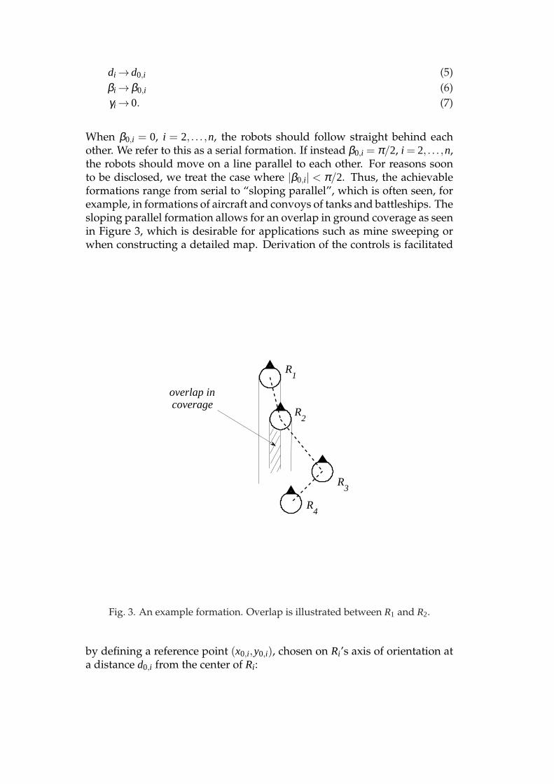
When β0,i = 0, i = 2, . . . ,n, the robots should follow straight behind eachother. We refer to this as a serial formation. If instead β0,i = π/2, i = 2, . . . ,n,the robots should move on a line parallel to each other. For reasons soonto be disclosed, we treat the case where |β0,i| < π/2. Thus, the achievableformations range from serial to “sloping parallel”, which is often seen, forexample, in formations of aircraft and convoys of tanks and battleships. Thesloping parallel formation allows for an overlap in ground coverage as seenin Figure 3, which is desirable for applications such as mine sweeping orwhen constructing a detailed map. Derivation of the controls is facilitated

−10 −5 0 5 10 15−12

−10

−8

−6

−4

−2

0

2

4

6

overlap in coverage

R3

R4

R1

R2

Fig. 3. An example formation. Overlap is illustrated between R1 and R2.

by defining a reference point (x0,i ,y0,i), chosen on Ri’s axis of orientation ata distance d0,i from the center of Ri :

x0,i = xi +d0,i cos(φi +β0,i)

y0,i = yi +d0,i sin(φi +β0,i).(8)

With this particular choice of reference point we obtain a point that can bedriven arbitrarily close to Ri−1 without causing the angle to target to be un-defined. The first formation control is presented in the following theorem:

Theorem 1 As t →∞, and with β0,i 6= π/2+mπ for any integer m, (x0,i(t),y0,i(t))converges to (xi−1(t),yi−1(t)) with the following control:

Control 1 :

vi =k

cosβ0,i

(

di cos(βi −β0,i)−d0,i +vi−1

kcos(γi +β0,i)

)

ωi =k

d0,i cosβ0,i

(

di sinβi −d0,i sinβ0,i −vi−1

ksinγi

)

.

(9)

Proof The proof is straightforward. In fact, let xe = x0,i − xi−1,ye = y0,i −yi−1, then we have

xe = xi +d0,i cos(φi +β0,i)−xi−1

ye = yi +d0,i sin(φi +β0,i)−yi−1,(10)

so that

xe

ye

=

vi cosφi −d0,iωi sin(φi +β0,i)−vi−1cosφi−1

vi sinφi +d0,iωi cos(φi +β0,i)−vi−1sinφi−1

=

cosφi −d0,i sin(φi +β0,i)

sinφi d0,i cos(φi +β0,i)

vi

ωi

−vi−1

cosφi−1

sinφi−1

. (11)

Now, by solving

cosφi −d0,i sin(φi +β0,i)

sinφi d0,i cos(φi +β0,i)

vi

ωi

=−k

xe

ye

+vi−1

cosφi−1

sinφi−1

(12)

for vi and ωi we obtain Control 1, which obviously yields the error dynamics

xe = −kxe

ye = −kye.(13)

�

As seen from Equation (13), the control gain k determines the rate of conver-gence to the desired configuration. In practice, of course, physical limita-tions will determine the upper bound for k. Also, due to the discretizationof the control in implementation, a too large gain may lead to overshoot.The value of k must therefore be tuned with respect to platform and dis-cretization method. By construction, Control 1 drives di to d0,i and βi to β0,i ,satisfying the control objectives (5) and (6). For the third control objective,consider the case ωi−1 = 0. With Control 1, the formation is driven to thesteady state di = d0,i , βi = β0,i . Then (4) becomes

γi =−vi−1

d0,i cosβ0,isinγi , (14)

with equilibria at γi = 0±π . For vi−1 > 0 and |β0,i|< π/2 we get

γi <0 if γi ∈ (0,π) (15)

γi >0 if γi ∈ (−π,0). (16)

In other words, with ωi−1 = 0, γi has a stable equilibrium at γi = 0 and un-stable equilibria at γi = ±π . Therefore, for bounded angular velocity ωi−1,γi stays close to zero.

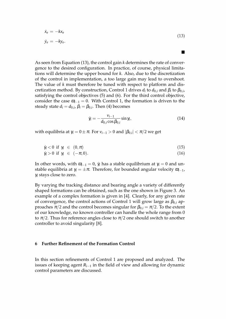
By varying the tracking distance and bearing angle a variety of differentlyshaped formations can be obtained, such as the one shown in Figure 3. Anexample of a complex formation is given in [4]. Clearly, for any given rateof convergence, the control actions of Control 1 will grow large as β0,i ap-proaches π/2 and the control becomes singular for β0,i = π/2. To the extentof our knowledge, no known controller can handle the whole range from 0to π/2. Thus for reference angles close to π/2 one should switch to anothercontroller to avoid singularity [8].

6 Further Refinement of the Formation Control

In this section refinements of Control 1 are proposed and analyzed. Theissues of keeping agent Ri−1 in the field of view and allowing for dynamiccontrol parameters are discussed.

6.1 Driving βi(t) to β0,i

Equation (13) shows that Control 1 is globally exponentially stable in termsof position errors. However, the control cannot guarantee that the angularerror |βi(t)− β0,i | decreases monotonically. Thus, if the sensors have onlylimited angular field of view, we may risk losing track of the target. There-fore, some strategy for active sensing is needed when using Control 1. Sucha strategy is further discussed in Section 7, where a switching Kalman filteris used as an observer whose input depends on which sensors of agent Ri

currently view agent Ri−1.

However, a slight modification of Control 1 does make |βi(t)−β0,i | decreasemonotonically. The ability to control βi in this manner means that agent Ri

can choose to keep agent Ri−1 in the field of view of some particular sensorsat all times, unless the reference value β0,i changes rapidly. The price we payis the loss of globality. The modified control is presented in the followingtheorem.

Theorem 2 Let

Control 2 :

vi =k

cosβi

(

di −d0,i cos(βi −β0,i)+vi−1

kcos(γi +βi)

)

ωi =k

di cosβi

(

di sinβi −d0,i sinβ0,i −vi−1

ksinγi

)

,

(17)

where k > 0, d0,i > 0, |β0,i| <π2 . Then for any βi(0) ∈ (−π

2 ,π2) and di(0) > 0,

|βi(t)−β0,i | tends to zero monotonically and di(t)−d0,i tends to zero.

Proof Define di = di cosβi − d0,i cosβ0,i and βi = βi − β0,i . Then we have,from Equations (2) - (3)

˙di = di cosβi −di βi sinβi =−vi +vi−1cosγi +diωi sinβi

˙βi = βi =−ωi +vidi

sinβi −vi−1di

sin(γi +βi).(18)

Now, plugging in Control 2 into (18) yields

˙di = −kdi

˙βi = −kd0,i cosβi

d0,i cosβ0,i + disinβi .

(19)

Since |di(t)| decreases monotonically, di(t)> 0∀t ≥ 0 due to the continuity of

the solution. Since˙βi =−k

d0,idi(t)

sinβi , it is easy to see that as long as |βi(0)|<π2 , |βi(t)−β0,i | decreases monotonically.

�

When β0,i is constant or slowly varying, Control 2 ensures that Ri−1 stayswithin the field of view of some of the sensors of Ri . However, some sce-narios may require a flexible formation, where β0,i changes rapidly to adaptto conditions in the environment. This would motivate the introduction ofsome active sensing scheme. In the next section, a formation control withdynamic control parameters is proposed.

6.2 Dynamic Control Parameters

A variety of formations can be obtained by altering the parameters d0,i andβ0,i . As Control 1 is globally stable for |β0,i| < π/2, switching between dif-ferent parameter values can be performed independently on-line for eachrobot. Under the assumption of directional sensors, a control with switch-ing reference values should be combined with active sensing. This is fur-ther discussed in Section 7, where a switching Kalman filter is proposed fortarget tracking applications.

In this section the stability of Control 1 with dynamic parameters d0,i(t),β0,i(t)is analyzed. According to Theorem 1, Control 1 is globally stable for con-stant d0,i and β0,i . For time varying d0,i(t) and β0,i(t), using the same con-trol input vi and ωi yields an additional nonlinear term in the error dy-namics due to the nonzero time derivatives of d0,i(t) and β0,i(t). Recall thatxe = x0,i −xi−1,ye = y0,i −yi−1. The derivatives are now

xe

ye

=−k

xe

ye

+

cos(φi +β0,i) −d0,i sin(φi +β0,i)

sin(φi +β0,i) d0,i cos(φi +β0,i)

d0,i

β0,i

. (20)

We see that rapid changes in d0,i(t) and β0,i(t) might affect stability of theerror dynamics. Denote by Φ(t) the nonlinear term of Equation (20). Thenthe error expression is

xe

ye

= e−kt

xe(0)

ye(0)

+∫ t

0e−k(t−s)Φ(s)ds. (21)

Note that, with ‖ · ‖ denoting the euclidean norm,

‖Φ(t)‖=

∥

∥

∥

∥

∥

∥

cos(φi +β0,i) −sin(φi +β0,i)

sin(φi +β0,i) cos(φi +β0,i)

d0,i

d0,i β0,i

∥

∥

∥

∥

∥

∥

=√

d20,i +d2

0,i β20,i .

(22)

Therefore, if there exists an M such that√

d20,i +d2

0,i β20,i ≤ M, ∀t ≥ 0, it holds

that∥

∥

∥

∥

∥

∥

xe

ye

∥

∥

∥

∥

∥

∥

≤

∥

∥

∥

∥

∥

∥

xe(0)

ye(0)

∥

∥

∥

∥

∥

∥

e−kt +Mk

1

1

(

1−e−kt)

, (23)

so that as t →∞ the right hand side of Equation (23) tends to M/k. Thus, withControl 1 and a given value of k, the error is bounded if d0,i(t), d0,i(t) and

β0,i(t) are chosen so that M/k is smaller than the sensor range. To eliminatethe static error, the following modified control should be used:

Theorem 3 For vi and ωi defined by Equation (9), the control

Control 3 :

vi = vi + ∆v

ωi = ωi + ∆ω(24)

with

∆v

∆ω

=−1

d0,i cosβ0,i

d0,id0,i

d0,i sinβ0,i + β0,id0,i cosβ0,i

(25)

results in the error dynamics (13).

Proof The proof is straightforward and follows from the fact that, withdynamic control parameters d0,i(t) and β0,i(t), the error dynamics are

xe = vi cosφi −vi−1cosφi−1+ d0,i cos(φi +β0,i)−d0,i(β0,i +ωi)sin(φi +β0,i)

ye = vi sinφi −vi−1sinφi−1+ d0,i sin(φi +β0,i)+d0,i(β0,i +ωi)cos(φi +β0,i).

(26)Replacing (vi ,ωi) with (vi + ∆v,ωi + ∆ω) yields

xe = (vi + ∆v)cosφi−vi−1 cosφi−1+d0,i cos(φi+β0,i)−d0,i(β0,i+ωi + ∆ω)sin(φi+β0,i)

ye = (vi + ∆v)sinφi−vi−1 sinφi−1+d0,i sin(φi+β0,i)+d0,i(β0,i+ωi + ∆ω)cos(φi+β0,i).

(27)

Now define

∆xe

∆ye

=

∆vcosφ + d0,i cos(φi +β0,i)−d0,i(β0,i +∆ω)sin(φi +β0,i)

∆vsinφi + d0,i sin(φi +β0,i)+d0,i(β0,i +∆ω)cos(φi +β0,i)

=

cosφi −d0,i sin(φi +β0,i)

sinφi d0,i cos(φi +β0,i)

∆v

∆ω

+

d0,i cos(φi +β0,i)−d0,iβ0,i sin(φi +β0,i)

d0,i sin(φi +β0,i)+d0,iβ0,i cos(φi +β0,i)

,

(28)

so that

xe

ye

=−k

xe

ye

+

∆xe

∆ye

. (29)

Now, since the control ∆v,∆ω defined by (25) solves

cosφi −d0,i sin(φi+β0,i)

sinφi d0,i cos(φi+β0,i)

∆v

∆ω

= −

d0,i cos(φi+β0,i)−d0,iβ0,i sin(φi+β0,i)

d0,i sin(φi+β0,i)+d0,iβ0,i cos(φi+β0,i)

,

(30)

the terms ∆xe,∆ye vanish and the resulting error dynamics are exponentiallystable. Note that the derivatives of d0,i(t) and β0,i(t) are completely knownsince they are control inputs.

�

Next, the switching Kalman filter is derived.

7 Active Sensing Through Switching Kalman Filters

To use Control 1 for agent Ri , we need to estimate the distance di , the angleβi , and the velocity vi−1 of Ri−1 from sensor measurements. When using di-rectional range sensors, the only information available is the distance fromeach sensor to Ri−1. di and βi may be computed directly from sensor data,but this is not the case for vi−1. In [19] a nonlinear observer is proposedfor this purpose. In this section, an alternative approach is introduced, en-abling the use of a linear observer in the form of a Kalman filter.

As we shall see, even though this is not required explicitly by the forma-tion controls, the Kalman filter needs an estimate of the global position ofthe target in order to estimate vi−1. Although this introduces extra com-putations, the method is appealing due to the desirable properties of theKalman filter, such as linearity, optimality and convergence.

As Control 1 does not guarantee monotonic convergence of βi , the observermust be robust to the scenario that agent Ri−1 moves out of the field ofview for some of the sensors of agent Ri . Using dynamic parameters, Con-trol 2 may also loose tracking for some directional sensors. We proposea switching Kalman filter for active sensing, and introduce the concept ofactive sensor pairs to obtain appropriate input to the Kalman filter.

The Khepera II, with its directional IR proximity sensors, is used as an ex-ample platform to illustrate the method. For localization, Khepera II usesodometry. Further down, expressions for di , βi , γi and vi−1 are computedfrom sensor measurements. First, a brief review of notation and recursionformulas for the Kalman filter is provided.

7.1 The Discrete Kalman Filter

In this section we introduce notation and review the Kalman recursions.Consider a discrete, time-invariant system with a state space vector xt gov-erned by the linear stochastic difference equation

xt = Axt−1+Bwt (31)

and a measurement yt ∈ Rm governed by

yt =Cxt +vt . (32)

The signals wt and vt are random process noise and measurement noise,respectively, and are assumed to be independent, gaussian noise with co-variance matrices

E(wtwTt ) = Qt

E(vtvTt ) = St .

(33)

Here, E(·) is the expectation value of (·). The discrete Kalman filter is anobserver that gives an estimate xt of the state xt at time step t, given the es-timate xt−1 and the observation yt , in a least squares sense. In other words,if we define the estimation error as

et = xt − xt , (34)

then the Kalman filter will give the estimate xt that minimizes E(eTt et). Now

let

Pt , E(eteTt ) (35)

denote the covariance matrix of xt . Then, given initial estimates x0 and P0,the discrete Kalman filter is the recursive process

x−t = Axt−1

P−t = APt−1AT +BTQt−1B

Kt = P−t CT

(

CP−t CT +Rt

)−1

xt = x−t +Kt(

yt −Cx−t)

Pt = (I −KtC)P−t .

(36)

Next, the application of the Kalman filter to target tracking is discussed.

7.2 Target tracking using the Kalman filter

Consider the problem of estimating the motion of the target Ri−1. Thisshould be done locally by Ri using odometry and the information availablefrom the sensor pairs p j , j = 1, . . . ,6, shown in Figure 4. A linear model isneeded for the kinematics of Ri−1 in order to apply a Kalman filter. There-fore, let the position (xi−1,yi−1) and motion (xi−1, yi−1) of Ri−1 constitute thestate vector:

x =(

xi−1 yi−1 xi−1 yi−1

)T. (37)

Since we assume that the follower Ri has no a priori information about thekinematics or trajectory of Ri−1, it is natural to represent the motion with anordinary random walk model:

x =

0 0 1 0

0 0 0 1

0 0 0 0

0 0 0 0

x +

0 0

0 0

1 0

0 1

w, (38)

where w = (xi−1 yi−1)T is the unknown acceleration of Ri−1, which is mod-

eled as gaussian noise. As (xi−1,yi−1) can be measured in the sense that theycan be computed from sensor measurements, we define the measurement yof the dynamic system (38) as

y =

1 0 0 0

0 1 0 0

x + v. (39)

where v is unknown, gaussian measurement noise. To enable applicationof the discrete Kalman filter, the system (38) - (39) is discretized using ansample time h. Denoting the discrete time steps with t, we get

xt+1 =

1 0 h 0

0 1 0 h

0 0 1 0

0 0 0 1

xt +

h2

2 0

0 h2

2

h 0

0 h

wt

yt =

1 0 0 0

0 1 0 0

xt + vt .

(40)

It is easy to show that this system is observable. The output of the Kalmanfilter is

x = (xi−1 yi−1 ˙xi−1 ˙yi−1)T , from which the velocity estimate vi−1 =

√

˙x2i−1+

˙y2i−1

is finally obtained. In the next section, y is derived from sensor measure-ments.

7.3 Computation of Kalman Filter Output

y in (39) can be derived from sensor data, using triangulation for pairs ofdirectional sensors, as follows. For the Khepera II we define 6 neighboringsensor pairs (Figure 4):

p1 = {s1 s2}, p2 = {s2 s3}, p3 = {s3 s4},

p4 = {s4 s5}, p5 = {s5 s6}, p6 = {s7 s8}.(41)

When there is no risk of confusion, we will use the notation sq to specifyboth the sensor indexed q∈ [1,8], and the global position of that sensor. Foran explanation of the notation used in this section, see Figure 6.

The IR sensors of the Khepera II measure reflected light intensity. The re-lation between light intensity and distance for the IR sensors depends onfactors such as ambient light and reflecting material. For the initial exper-iments presented in Section 8, the measured relation is shown in Figure 5.Let δq be the measured distance to the target from sensor sq, and define the

p3

p4

p5

p6

p2

p1

60 mms1

s2

s3 s

4

s5

s6

s7 s

8

Fig. 4. The sensor pairs of Khepera II.

0 100 200 300 400 500 600 700 800 900 1000 11000

20

40

60

80

100

120

140

160

sensor reading

dist

ance

(m

m)

sensor 1sensor 2sensor 3sensor 4

Fig. 5. The relation between sensor output and distance, as measured by the ex-perimental setup in Section 8

.

distance δq from sensor sq to (xi−1,yi−1):

δq , δq+ r. (42)

Here, r denotes the radius of Ri−1. Let p j = {sq,sq−1}, ∆sj = ‖sq− sq−1‖and define, using the law of cosines, the angle ψ j such that

δ 2q−1 = ∆s2

j +δ 2q −2∆sjδqcosψ j . (43)

Denote by y j the target position estimate associated with p j . All variablesare defined in a local coordinate system O′ with x-axis parallel to the differ-ence vector sq−sq−1 as shown in Figure 6. Expressed in O′, we obtain

−3.5 −3 −2.5 −2 −1.5 −1 −0.5 0 0.5 1 1.5−1

−0.5

0

0.5

1

1.5

2

2.5

3

δq−1

∆ sj

O’ x’

y’

rr δ

q

∆ x’

∆ y’

sq

sq−1

ψj

Fig. 6. Notation for computing the position of Ri−1 from sensor measurements.Here sq and sq−1 form the sensor pair p j .

∆x′j = δqcosψ j

∆y′j = δqsinψ j .(44)

This means that the position of the target, as measured by p j , in the frameO′ is

y′j =(

x′q−∆x′j y′q+∆y′j

)T= (x′i−1 y′i−1)

T (45)

where (x′q,y′q) are the coordinates of the sensor sq in the local frame. Ex-

pressed in the global coordinate system, we get

y j =

cosθ −sinθ

sinθ cosθ

x′i−1

y′i−1

+

xi

yi

, (46)

where θ is the rotation of O′ compared to the global frame. θ and (xi ,yi)are obtained from the odometry of Ri . Before computing control inputs, acritical issue is to decide from which senor pairs to record measurements.This is discussed in the next section, and a formalization of the procedureis provided.

7.4 Switching Kalman Filters

In this section we derive a switching Kalman filter suitable for target track-ing using directional sensors. It is clear from Figure 2 that each sensor has

a limited field of view. We say that a sensor is active if the target is in itsfield of view. If a Kalman filter Fj is designed for each sensor pair p j andthey are allowed to act on the discretized system (40), Fj will only give afair estimation if both sensors in p j are active. Further, note that (43) and(44) yield

∆y′j =√

δ 2q −∆x′2j = δq

√

1−

(

∆s2j+δ 2

q−δ 2q−1

2∆sj δq

)2(47)

which is imaginary for (∆s2j + δ 2

q − δ 2q−1/2∆sjδq)

2 > 1. Naturally, the true

distance ∆y′j is a real number. However, the estimate computed from (47)can be imaginary if too much measurement noise is present in the sensorreadings δq and δq−1. We will therefore use the following definition.

Definition 1 A filter Fj is activeat time step t if and only if

(1) Both sensors in the associated sensor pair p j are active(2) For measurements from the sensor pair p j , it holds that

(

∆s2j +δ 2

q −δ 2q−1

2∆sjδq

)2

< 1. (48)

In order to estimate the movement of Ri−1, Ri should only pay attentionto the output of active filters. Which filters Fj that are active at each timestep will vary with the path of the target and the tracking parameters. Thismotivates the use of a switching Kalman filter.

The switching Kalman filter consists of the subfilters Fj , which all run inparallel to each other. At each time step, the estimates x j,t from the activesubfilters are merged into an estimate xt for the switching filter. xt can beeither a linear combination of the state estimates from the active filters, orthe best estimate x j,t with respect to some criterion.

A summary of the switching Kalman filter scheme follows in Algorithm 7.1.

Algorithm 7.1 Target Tracking with a Switching Kalman FilterFor each follower agent Ri , at each time step t:

(1) Record, using odometry, the agent’s own position at time t: (xi,t ,yi,t ,φi,t).(2) Record range measurements from the IR sensors. If sq−1 and sq both get read-

ings, the associated sensor pair p j is added to the list of candidates for activefilters.

(3) Check condition (48). If (48) holds for p j , this sensor pair is added to thefinal list of active sensor pairs.

(4) Compute y j,t for all active sensor pairs using (42) - (46).(5) Apply the Kalman filter (36) to the system (40) using y j,t to obtain estimates

x j,t for all active filters.(6) Compute or choose the final state estimate xt = (xi−1,t yi−1,t ˙xi−1,t ˙yi−1,t)

T

from the estimates x j,t .(7) Compute

vi−1,t =√

˙x2i−1,t +

˙y2i−1,t (49)

di,t =√

(xi−1,t −xi,t)2+(yi−1,t −yi,t)2 (50)

βi,t = tan−1 yi−1,t −yi,t

xi−1,t −xi,t−φi,t (51)

φi−1,t = tan−1 yi−1,t − yi−1,t−1

xi−1,t − xi−1,t−1(52)

γi,t = φi,t −φi−1,t . (53)

(8) Compute and apply control inputs vi,t and ωi,t from Control 1, Control 2 orControl 3.

In the next section, the controls discussed in previous sections are demon-strated in experiments and simulations.

8 Experiments and Simulations

In this section, initial results from experiments and simulations are pro-vided. The results in this section serve to illustrate the theoretical results inprevious sections. An extensive experimental evaluation remains for futurework and will be further discussed in Section 9. First, the outcome of exper-iments using Control 1 and Algorithm 7.1 are reported. Then, simulationresults for Control 2 and Control 3 are included to demonstrate advantagesof refining the control.

8.1 Experiments: Control 1 and Algorithm 7.1

The platform used in the experiments is the Khepera II (Figure 2) which hasunicycle kinematics and 8 directional IR sensors. The sensors have a rangeof up to 100 mm but the quality of data is highly sensitive to factors such asambient light. For localization, the Khepera II uses odometry.

Algorithm 7.1 was used to obtain position and velocity estimates. Theswitching strategy was to choose xt as the estimate x j,t among the outputs

of the active filters Fj that differed the least from the previous estimate xt−1.This is a rough and simple strategy, best suited for constant or slowly vary-ing parameters. More sophisticated strategies should be investigated infuture work.

The experiments were performed with a setup of one leader (R1) followinga predefined path, and one follower (R2). The platforms were controlledthrough an interface in MATLAB. No communication occurred between theagents.

Results are shown for robustness of a rigid formation as well as for switch-ing bearing angle. The figures in this section contain plots of ∆d2 and β2

computed from the Kalman filter output. Note that the scaling differs some-what between plots, depending on the magnitude of the deviations of thecurves from the reference values.

Robustness of Control A.1

To investigate the robustness of Control 1, R1 followed a predefined path atconstant speed, and R2 tracked R1 with a given reference angle, β0,2, and areference distance of d0,2 = 120 mm (from center to center).

The formation error ∆d2 ≡ d2−d0,2 and angle β2, together with the trajecto-ries of the robots, are shown in Figure 7 - 8 for β0,2 = 0 rad and β0,2 = π/6 radrespectively. For β0,2 = 0 rad, β2 converges nicely and stays at 0 rad aftera transient of about 15 s. β0,2 = π/6 rad is a more challenging case for theKhepera II, as this angle lies at the edge of the field of view for two sensors(s2 and s3 in Figure 4). As seen in Figure 8, β2 fluctuates around its referencevalue and does not converge. This is due to the fact that for this challengingangle, the active filter switches back and forth between F2, F3, and some-times F1 (see Figure 4). In addition, the drifting error in the odometry usedfor localization contributes to measurement uncertainties. To reduce oscil-lations, a more sophisticated switching strategy, such as a weighted meanestimate from several filters, should be applied. This is an issue for furtherstudy. However, despite fluctuations, R2 is able to follow R1, R1 remainswithin the sensor range of R2 at all times, and the errors are bounded.

Robustness for switching β0

To investigate the robustness of a switch of the reference angle, the samesetup as in Section 8.1 was used. Again, R1 followed a predefined path withconstant speed, and R2 tracked R1 with reference angle β0,2 = 0 rad, and areference distance of d0,2 = 120 mm. The reference angle was switched toβ0,2 = π/6 rad at t = 10s, and then switched back to β0,2 = 0 rad at t = 60s.

−100 0 100 200 300

0

0.01

0.02

0.03

0.04

0.05

0.06

x

y

Paths for β0,2

= 0 rad

Robot 1Robot 2

10 20 30 40 50 60 70

−5

0

5

10

t

∆ d2

Error in d2 for β

0,2 = 0 rad

0 10 20 30 40 50 60 70−2.5

−2

−1.5

−1

−0.5

0

0.5

1x 10−4

t

β 2

β2 for β

0,2 = 0 rad

β2

β0,2

Fig. 7. Robustness of Control A.1: β0 = 0 rad. Top: The trajectories of the plat-forms. Middle: The difference ∆d2(t) [mm]. Bottom: The angle β2(t) rad and thebearing angle β0,2(t) rad.

The formation error ∆d2 and angle β2 are shown, together with the trajecto-ries, in Figure 9. After a transient of roughly 20 s, ∆d2 decreases and fluctu-ates around a small static error despite switch in β0,2. R2 responds quicklyto the change in β0,2 and although fluctuations are present, we observe nostatic error in β2. R1 remains withing the field of view of R2 throughout theexperiment, and the errors remain bounded.

−100 0 100 200 300 400−80

−60

−40

−20

0

x

y

Paths for β0 = π/6 rad

Robot1Robot2

0 10 20 30 40 50 60 70

−20

0

20

40

60

80

t

∆ d2

Error in d2 for β

0,2 = π/6 rad

0 10 20 30 40 50 60 70

0

0.5

1

1.5

t

β 2

β2 for β

0,2 = π/6 rad

β2

β0,2

Fig. 8. Robustness of Control A.1: β0 = π/6 rad. Top: The trajectories of theplatforms. Middle: The difference ∆d2(t) [mm]. Bottom: The angle β2(t) rad andthe bearing angle β0,2(t) rad.

8.2 Simulations: Control 2

To demonstrate the usefulness of Control 2, simulations were carried out fortwo agents R1 and R2 using Control 1 and Control 2, which drives βi −β0,i

to zero monotonically. The agents were modeled as unicycle platforms. Forv1 = 10, ω1 = π/3, k= 1, β0,2 = π/7, d0,2 = 1,

−100 0 100 200 300 400 500 600 700−70

−60

−50

−40

−30

−20

−10

0

x

y

Paths for switching β0

Robot1Robot2

20 40 60 80 100

0

20

40

60

80

100

t

∆ d2

Error in d2 for swithcing β

0,2

0 20 40 60 80 100

−1

−0.5

0

0.5

1

1.5

2

t

β 2

β2 for switching β

0,2

β2

β0,2

Fig. 9. Robustness for switching β0: Experiment with switch from β0 = 0 radto β0 = π/6 rad. Top: The trajectories of the platforms. Note that, since R2 tracksR1 at a non-zero angle for t ∈ [10,60], its track deviates from that of R1. Middle:The difference ∆d2(t) [mm]. Bottom: The angle β2(t) rad and the bearing angleβ0,2(t) rad.

(x1,y1,φ1) = (0,0,0), (x2,y2,φ2) = (−0.97,−0.70,π/10) error convergence isstudied. The measured entities are the deviations from reference valuesof control parameters (d2 − d0,2 and β2 − β0,2), and position error (xe andye). Although all errors converge to 0, they do not do so monotonically forboth controls. Results are plotted in Figures 10 - 12. Figure 10 shows the

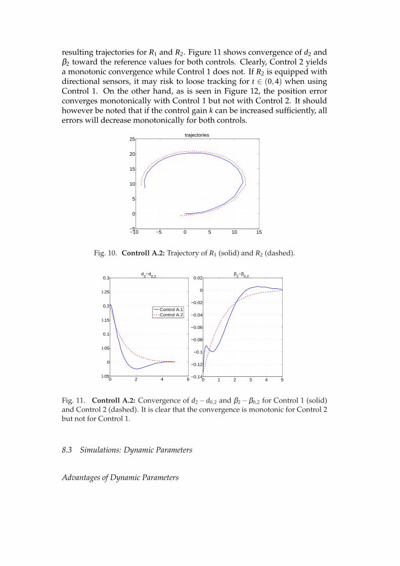
resulting trajectories for R1 and R2. Figure 11 shows convergence of d2 andβ2 toward the reference values for both controls. Clearly, Control 2 yieldsa monotonic convergence while Control 1 does not. If R2 is equipped withdirectional sensors, it may risk to loose tracking for t ∈ (0,4) when usingControl 1. On the other hand, as is seen in Figure 12, the position errorconverges monotonically with Control 1 but not with Control 2. It shouldhowever be noted that if the control gain k can be increased sufficiently, allerrors will decrease monotonically for both controls.

−10 −5 0 5 10 15−5

0

5

10

15

20

25trajectories

Fig. 10. Controll A.2: Trajectory of R1 (solid) and R2 (dashed).

0 2 4 6−0.05

0

0.05

0.1

0.15

0.2

0.25

0.3d

2−d

0,2

0 1 2 3 4 5−0.14

−0.12

−0.1

−0.08

−0.06

−0.04

−0.02

0

0.02β

2−β

0,2

Control A.1Control A.2

Fig. 11. Controll A.2: Convergence of d2−d0,2 and β2−β0,2 for Control 1 (solid)and Control 2 (dashed). It is clear that the convergence is monotonic for Control 2but not for Control 1.

8.3 Simulations: Dynamic Parameters

Advantages of Dynamic Parameters

0 1 2 3 4 5−0.25

−0.2

−0.15

−0.1

−0.05

0

0.05

0.1x

e

0 1 2 3 4 5−0.06

−0.05

−0.04

−0.03

−0.02

−0.01

0

0.01

0.02

0.03y

e

Control A.1Control A.2

Fig. 12. Controll A.2: Convergence of xe and ye for Control 1 (solid) and Control 2(dashed). It is clear that the convergence is monotonic for Control 1 but not forControl 2.

To demonstrate potential advantages of dynamic control parameters, weconsider a scenario where the formation strives to stay on the same path asthe leader at all times. We defined dynamic control parameters d0,i(t) andβ0,i(t) such that, given the path of agent Ri−1 up until time t, agent Ri shouldsteer toward a position located on that path such that the distance d0,i(t) ismaximized while the area shown in Figure 13 is smaller than a tolerancevalue Amax. Simulations were performed for a team of 5 agents using first

x (t), y (t)i−1 i−1

d

f

Ri−1

Ri

y

x

Area between d and path

i−1 i−1δ δx (t− t), y (t− t)

β

Fig. 13. Advantages of Dynamic Parameters: d0,i(t) is chosen as the maximumdistance that keeps the tinted area smaller than Amax.

dynamic, and then constant, d0,i and β0,i and results were compared. Forboth cases we used Control 1. The leader agent R1 traveled along a pre-defined path, which is unknown to the followers. The simulation setup isillustrated in Figure 14. For the dynamic parameters, letting Amax= 0.005resulted in a mean inter-agent distance of 1.19 length units. In the case withconstant parameters, we use reference angle 0 rad and reference distanceequal for all agents. This distance was chosen as d0,i = 1.19, i = 2, . . . ,5 toget as fair a comparison as possible. For both controls, we used the gain

0 5 10 15 201

2

3

4

5

6

75 agents servoing a path

Fig. 14. Advantages of Dynamic Parameters: A team of one leader and 4 followeragents tracking a path.

k = 1. At each time step, the deviation for Ri from the path of Ri−1 wasmeasured as

devi = minτ∈(0,t]

‖Ri−1(τ)− (xi(t),yi(t))‖. (54)

Results are shown in Figures 15 - 18. Figures 15 - 16 show a significantimprovement in path following using dynamic parameters. Figures 17 -18 show how d0,i and β0,i vary for the dynamic parameter control. Highcurvature parts of the path cause the formation to contract to enable saferpath following.

0 5 10 15 201

2

3

4

5

6

7

Dynamic d0, β

0

Path of R1 (solid), tracks of R

2,...,R

5 (dashed)

0 5 10 15 201

2

3

4

5

6

7

Constant d0, β

0

Fig. 15. Advantages of Dynamic Parameters: Tracks (dashed) for the followeragents. Left: Constant d0,i and β0,i . Right: Dynamic d0,i and β0,i .

Control 3

Finally, an example is included to illustrate the improvement of the errordynamics with Control 3. We used two agents and defined d0,2(t) and β0,2(t)

0 500 1000 1500 20000

0.1

0.2

0.3

0.4

0.5

0.6

0.7

0.8

dev 2

t

deviations from path of Ri−1

0 500 1000 1500 20000

0.1

0.2

0.3

0.4

0.5

0.6

0.7

0.8

dev 3

t

0 500 1000 1500 20000

0.1

0.2

0.3

0.4

0.5

0.6

0.7

0.8

dev 4

t0 500 1000 1500 2000

0

0.1

0.2

0.3

0.4

0.5

0.6

0.7

dev 5

t

dynamic parametersconstant parameters

Fig. 16. Advantages of Dynamic Parameters: Deviations from the path of Ri−1 forthe four followers.

0 500 1000 1500 20000

0.5

1

1.5

2

2.5

3

d 0,2

t

dynamic d0

0 500 1000 1500 20000

0.5

1

1.5

2

2.5

3

d 0,3

t

0 500 1000 1500 20000

0.5

1

1.5

2

2.5

3

3.5

4

d 0,4

t0 500 1000 1500 2000

0

1

2

3

4

5

d 0,5

t

Fig. 17. Advantages of Dynamic Parameters: Dynamic d0,i .

by

d0,2 = 0.1cos(45β0,2)

β0,2 = 0.001

d0,2(0) = 0.5

β0,2(0) = π/7.

(55)

0 500 1000 1500 2000−0.4

−0.3

−0.2

−0.1

0

0.1

0.2

0.3

β 0,2

t

dynamic β0

0 500 1000 1500 2000−0.4

−0.3

−0.2

−0.1

0

0.1

0.2

0.3

β 0,3

t

0 500 1000 1500 2000−0.4

−0.3

−0.2

−0.1

0

0.1

0.2

0.3

β 0,4

t0 500 1000 1500 2000

−0.4

−0.3

−0.2

−0.1

0

0.1

0.2

0.3

β 0,5

t

Fig. 18. Advantages of Dynamic Parameters: Dynamic β0,i .

The resulting functions d0,2(t) and β0,2(t) are shown in Figure 19. For v1 =

0 5 10 15

0.35

0.4

0.45

0.5

0.55

0.6

0.65

d0,2

0 5 10 150.448

0.45

0.452

0.454

0.456

0.458

0.46

0.462

0.464

0.466

β0,2

Fig. 19. Control 3: The dynamic parameters resulting from Equation (55). Left:d0,2(t). Right: β0,2(t).

10, ω1= π/3, k= 1, β0,2(0)= π/7, d0,2(0)= 1, (x1,y1,φ1)= (0,0,0), (x2,y2,φ2)=(−0.97,−0.70,π/10), we let R2 track R1 using Control 1, Control 2, and Con-trol 3. The gain k = 1 was used for all three cases. Results are shown inFigures 20 - 21. It is clear from Figure 20 that both Control 1 and Control 2yield static or even increasing errors in d2 and β2, while Control 3 drivesthe errors to zero. The same behavior is apparent for the errors xe and ye,shown in Figure 21.

0 5 10 15−0.1

0

0.1

0.2

0.3

0.4

0.5

0.6

d2−d

0,2

0 5 10 15−0.3

−0.25

−0.2

−0.15

−0.1

−0.05

0

0.05β

2−β

0,2

Control A.1Control A.2Control A.3

0 5 10 15−0.06

−0.04

−0.02

0

0.02

0.04

0.06

0.08

0.1d

2−d

0,2 CLOSEUP

0 5 10 15−0.01

−0.008

−0.006

−0.004

−0.002

0

0.002

0.004

0.006

0.008

0.01β

2−β

0,2

Control A.1Control A.2Control A.3

Fig. 20. Control 3: Left: d2− d0,2(t). Right: β2− β0,2(t). Top: full scale. Bottom:closeup view.

0 5 10 15

−0.6

−0.5

−0.4

−0.3

−0.2

−0.1

0

0.1x

e

0 5 10 15−0.4

−0.35

−0.3

−0.25

−0.2

−0.15

−0.1

−0.05

0

0.05y

e

Control A.1Control A.2Control A.3

Fig. 21. Control 3: Left: xe(t). Right: ye(t).

9 Conclusion

In this paper, cascaded controls were proposed for formations of autonomousagents. The controls are based on feedback from directional and noise con-taminated range sensors, and a switching Kalman filter was introduced to

enable target tracking for sensors with limited field of view. Theoreticalresults testified to stability and robustness, as well as flexibility, of the con-trols. Initial results from experiments and simulations were provided toillustrate the theoretical results. Combined with behaviors like obstacleavoidance and failure detection, the formation controls proposed in thispaper are suitable for applications such as servoing, surveillance and map-ping.

Future work includes a thorough experimental evaluation of the proposedcontrol algorithms. Issues of interest are for instance scalability and robust-ness with respect to noisy measurements, and refinement of the switchingcriterion for the Kalman filer algorithm. A comparative study should alsobe made in order to evaluate the proposed controls in contrast to for in-stance the hybrid control proposed in [5], and the Kalman filter approachin contrast to the non-linear observer in [19].

References

[1] C.W. Reynolds, Flocks, Herds, and Schools: A Distributed Behavioral Model,Computer Graphics, vol. 21, no. 4, pp. 25–34, 1987.

[2] T. Balch and R.C. Arkin, Behavior-based formation control for multirobotteams, Robotics and Automation, IEEE Trans. on, vol. 14, no. 6, pp. 926–939,1998.

[3] M. Egerstedt and Xiaoming Hu, Formation constrained multi-agent control,Robotics and Automation, IEEE Trans. on, vol. 17, no. 6, pp. 947–951, 2001.

[4] T. Gustavi and X. Hu, Formation Control for Mobile Robots with LimitedSensor Information, Proc. of IEEE International Conference on Robotics andAutomation (ICRA), pp. 367–393, 2005.

[5] David J. Naffin, Gaurav S. Sukhatme, and Mehmet Akar, Lateral andLongitudinal Stability for Decentralized Formation Control, Proceedings ofthe International Symposium on Distributed Autonomous Robotic Systems,pp. 421-430, June 2004.

[6] N.E. Leonard and E. Fiorelli, Virtual leaders, artificial potentials andcoordinated control of groups, Proc. of the 40th IEEE Conference on Decisionand Control (CDC), vol. 3, no. pp. 296–2973, 2001.

[7] N.E. Leonard, P. Ogren, and E. Fiorelli, Formations with a mission:stable coordination of vehicle group maneuvers, International Symposium onMathematical Theory of Networks and Systems (MTNS), 2002.

[8] M Karasalo T Gustavi, X Hu, Formation adaptation with limited sensorinformation, invited paper, Proc. of Chinese Control Conference (CCC), 2005.

[9] H.G. Tanner, G.J. Pappas, and V. Kumar, Leader-to-formation stability, IEEETrans. on Robotics and Automation, vol. 20, no. 3, pp. 443–455, 2004.

[10] M. Egerstedt, X. Hu, and A. Stotsky, Control of Mobile Platforms Using aVirtual Vehicle Approach, IEEE Trans. Automatic Control, vol. 46, no. 11, 2001.

[11] A.K. Das, R. Fierro, V. Kumar, J.P. Ostrowski, J. Spletzer, and C.J. Taylor,A vision based formation control framework, IEEE Trans. on Robotics andAutomation, vol. 18, pp. 813–825, 2002.

[12] J. Lawton, R. Beard, and B. Young, A entralized Approach to FormationManuervers, IEEE Trans. on Robotics and Automation, vol. 19, pp. 933–941, 2003.

[13] M. Mazo , A. Speranzon, K.H. Johansson, and X. Hu, Multi-Robot Trackingof a Moving Object Using Directional Sensors, Proc. of IEEE InternationalConference on Robotics and Automation (ICRA), 2004.

[14] R. Olfati-Saber and R.M. Murray, Graph Rigidity and Distributed FormationStabilization of Multi-Vehicle Systems, Proc. of IEEE Conference on Decision andControl (CDC), 2002.

[15] A. Jadbabaie, J. Lin and A. S. Morse, Coordination of groups of mobileautonomous agents using nearest neighbor rules, IEEE Trans. Automat. Control,vol. 48, no. 6, pp. 988–1001, 2003.

[16] K.D. Murphy, Switching Kalman Filter, Technical Report, Compaq CambridgeResearch Laboratory, 1998.

[17] R. Vidal, O. Shakernia, and S. Sastry, Formation Control of NonholonomicMobile Robots with Omnidirectional VisualServoing and Motion Segmentation, Proc. of IEEE International Conference onRobotics and Automation (ICRA), pp. 584–589, 2003.

[18] E. Bicho and S. Monteiro, Formation control for multiple mobile robots: anon-linear attractor dynamics approach, Proc. of the IEEE/RSJ InternationalConference on Intelligent Robots and Systems (IROS), pp. 2016–2022, 2003.

[19] T. Gustavi and X.Hu, Observer Based Leader-Following Formation Controlusing On-Board Sensor Information, IEEE Trans. on Robotics, vol. 24, no. 6, pp.1457–1462, 2008.

[20] C.A. Reeder, D.L. Odell, A. Okamoto, M.J. Anderson, and D.B. Edwards, Two-hydrophone heading and range sensor applied to formation-flying for AUVs,Proc. of MTTS/IEEE TECHNO-OCEAN ’04, pp. 517–523, 2004.

[21] S. Kim, C. Ryoo, K. Choi, and C. Park, Multi-vehicle formation using range-only measurement, Proc. of IEEE International Symposium on Circuits andSystems (ICCAS), pp. 2104–2109, 2007.